Neural Language Modeling for Contextualized Temporal Graph Generation

Abstract

This paper presents the first study on using large-scale pre-trained language models for automated generation of an event-level temporal graph for a document. Despite the huge success of neural pre-training methods in NLP tasks, its potential for temporal reasoning over event graphs has not been sufficiently explored. Part of the reason is the difficulty in obtaining large training corpora with human-annotated events and temporal links. We address this challenge by using existing IE/NLP tools to automatically generate a large quantity (89,000) of system-produced document-graph pairs, and propose a novel formulation of the contextualized graph generation problem as a sequence-to-sequence mapping task. These strategies enable us to leverage and fine-tune pre-trained language models on the system-induced training data for the graph generation task. Our experiments show that our approach is highly effective in generating structurally and semantically valid graphs. Further, evaluation on a challenging hand-labeled, out-of-domain corpus shows that our method outperforms the closest existing method by a large margin on several metrics. We also show a downstream application of our approach by adapting it to answer open-ended temporal questions in a reading comprehension setting.

1 Introduction

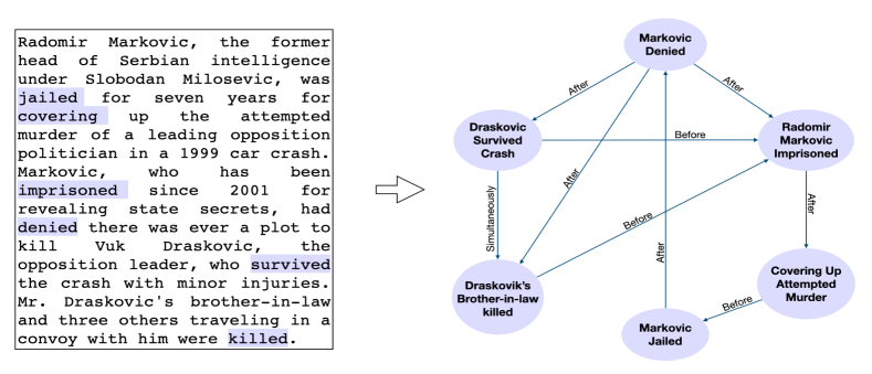
Figure 1: Task overview: given a document (left), automatically extract a temporal graph (right).

Temporal reasoning is crucial for analyzing the interactions among complex events and producing coherent interpretations of text data  Duran et al. (2007). There is a rich body of research on the use of temporal information in a variety of important application domains, including topic detection and tracking Makkonen et al. (2003), information extraction Ling and Weld (2010), parsing of clinical records  Lin et al. (2016), discourse analysis Evers-Vermeul et al. (2017), and question answering Ning et al. (2020).

Graphs are a natural choice for representing the temporal ordering among events, where the nodes are the individual events, and the edges capture temporal relationships such as “before”, “after” or “simultaneous”. Representative work on automated extraction of such graphs from textual documents includes the early work by Chambers and Jurafsky (2009), where the focus is on the construction of event chains from a collection of documents, and the more recent caevo Chambers et al. (2014) and Cogcomptime Ning et al. (2018), which extract a graph for each input document instead. These methods focus on rule-based and statistical sub-modules to extract verb-centered events and the temporal relations among them. As an emerging area of nlp, large scale pre-trained language models have made strides in addressing challenging tasks like commonsense knowledge graph completion Bosselut et al. (2019) and task-oriented dialog generation Budzianowski and Vulić (2019). These systems typically fine-tune large language models on a corpus of a task-specific dataset. However, these techniques have not been investigated for temporal graph extraction.

This paper focuses on the problem of generation of an event-level temporal graph for each document, and we refer to this task as contextualized graph generation. We address this open challenge by proposing a novel reformulation of the task as a sequence-to-sequence mapping problem Sutskever et al. (2014), which enables us to leverage large pre-trained models for our task. Further, different from existing methods, our proposed approach is completely end-to-end and eliminates the need for a pipeline of sub-systems commonly used by traditional methods.

We also address a related open challenge, which is a prerequisite to our main goal: the difficulty of obtaining a large quantity of training graphs with human-annotated events and temporal relations. To this end, we automatically produce a large collection of document-graph pairs by using caevo, followed by a few rule-based post-processing steps for pruning and noise reduction. We then encode the graph in each training pair as a string in the graph representation format dot, transforming the text-to-graph mapping into sequence-to-sequence mapping. We fine-tune gpt-2 on this dataset of document-graph pairs, which yields large performance gains over strong baselines on system generated test set and outperforms caevo on TimeBank-Dense Cassidy et al. (2014) on multiple metrics. Figure 1 shows an example of the input document and the generated graph by our system. In summary, our main contributions are:

1. We present the first investigation on using large pre-trained language models for contextualized temporal event graph generation by proposing a new formulation of the problem as a sequence-to-sequence mapping task.

2. We address the difficulty of obtaining a large collection of human-annotated graphs, which is crucial for effective fine-tuning of pre-trained models, by automatically producing a collection of 89,000 document-graph pairs.

3. Our experimental results on both the system-generated test set (which allows us to compare the relative performance of different models) and a hand-labeled, out-of-domain dataset (TimeBank-Dense), show the advantage of our proposed approach over strong baselines. Further, we show that our approach can help in generating plausible answers for open ended-temporal questions in a reading comprehension dataset, Torque Ning et al. (2020).

2 Related Work

Temporal Graph Extraction

Tempeval-3 UzZaman et al. (2013) introduced the task of temporal graph extraction as “the ultimate task for evaluating an end-to-end system that goes from raw text to TimeML annotation”. Notable systems developed in response include caevo Chambers et al. (2014), followed by the more recent Cogcomptime Ning et al. (2018). Both caevo and Cogcomptime use several statistical and rule-based methods like event extractors, dependency parsers, semantic role labelers, and time expression identifiers for the task. Our work differs from these systems in both the methodology and desired result in the following ways: i) Instead of using specialized sub-systems, we transform the task into a sequence-to-sequence mapping problem and use a single language model to generate such temporal graphs in an end-to-end fashion from text, subsuming all the intermediate-steps. ii) We develop our system using a corpus of 89,000 documents, which is $\sim$ 300x larger compared to datasets used by caevo (36 documents) and Cogcomptime on (276 documents); iii) We remove the noisy events included by caevo, but do not limit the extracted events to any specific semantic axis as done by Cogcomptime; and finally, iv) Our method generates graphs where the nodes are not simple verbs but augmented event phrases, containing the subject and the object of each verb. We use caevo over Cogcomptime to generate a large-scale corpus for our task and to evaluate our system for the following reasons: i) We found caevo to be much more scaleable, a critical feature for our task of annotating close to 100k documents, ii) caevo over-generates (and not excludes) verbs from its output, giving us the flexibility to filter out noisy events without inadvertently missing out on any critical events. However, our method makes no assumption specific to caevo and is adaptable to any other similar system (including Cogcomptime).

Temporal relation extraction

We note that the problem of temporal graph extraction is different from the more popular task of Temporal relation extraction (Temprel), which deals with classifying the temporal link between two already extracted events. State of the art Temprel systems use neural methods Ballesteros et al. (2020); Ning et al. (2019b); Goyal and Durrett (2019); Han et al. (2019); Cheng and Miyao (2017), but typically use a handful of documents for their development and evaluation. Vashishtha et al. (2019) are a notable exception by using Amazon Mechanical Turks to obtain manual annotations over a larger dataset of 16,000 sentences. We believe that the techniques presented in our work can be applied to scale the corpus used for training Temprel systems.

Language Models for Graph Generation

Recently, Bosselut et al. (2019) proposed comet, a system that fine-tunes gpt (Radford et al., 2018) on commonsense knowledge graphs like atomic Sap et al. (2019) and conceptnet (Speer et al., 2017) for commonsense kb completion. Similar to comet, we adopt large-scale language models for such a conditional generation of text. However, our task differs from comet in the complexity of both the conditioning text and generated text: we seek to generate temporal graphs grounded in a document, whereas comet generates a short event/concept phrase conditioned on a relation and an input event/concept phrase. Madaan et al. (2020) and Rajagopal et al. (2021) aim to generate event influence graphs grounded in a situation. Similar to this work, these methods rely on pre-trained language models to generate informative structures grounded in text. Different from us, these methods break the generation process into a sequence of natural language queries. Each query results in an event node, which are finally assembled into a tree. In contrast, we propose a method to directly generate graphs with arbitrary topology from text. Additionally, the events generated by these methods are not present in text making event event prediction, rather than event extraction as their primary focus. You et al. (2018) formulate graphs as a sequence for learning generative models of synthetic and real-world graphs. Similar to their work, we formulate graph generation as an auto-regressive task. However, our goal is the conditional generation of temporal graphs, and not learning unconditional generative distributions. Finally, inspired by recent trends Raffel et al. (2019), we do not make any graph specific modifications to the model or the decoding process and formulate the problem as a straightforward sequence-to-sequence mapping task. While our approach does not rely on any particular language model, it would be interesting to see the gains achieved by the much larger gpt-3 Brown et al. (2020) on the dataset produced by our method.

3 Deriving Large-scale Dataset for the Temporal Graph Generation

Definitions and Notations: Let $\mathbf{G}(\mathbf{V},\mathbf{E})$ be a temporal graph associated with a document $\mathbf{D}$, such that vertices $\mathbf{V}$ are the events in document $\mathbf{D}$, and the edges $\mathbf{E}$ are temporal relations (links) between the events. Every temporal link in $\mathbf{E}$ takes the form $r(e_{q},e_{t})$ where the query event $e_{q}$ and the target event $e_{t}$ are in $\mathbf{V}$, and $r$ is a temporal relation (e.g., before or after). In this work, we undertake two related tasks of increasing complexity: i) Node generation, and ii) Temporal graph generation:

Task 1: Node Generation: Let $r(e_{q},e_{t})$ be an edge in $\mathbf{E}$. Let $C_{r}$ be the set of sentences in the document $\mathbf{D}$ that contains the events $e_{q}$ or $e_{t}$ or are adjacent to them. Given a query consisting of $C_{r}$, $r$, and $e_{q}$, generate $e_{t}$.

Task 2: Temporal Graph Generation: Given a document $\mathbf{D}$, generate the corresponding temporal graph $\mathbf{G}(\mathbf{E},\mathbf{V})$.

Figure 1 illustrates the two tasks. Task 1 is similar to knowledge base completion, except that the output events $e_{q}$ are generated, and not drawn from a fixed set of events. Task 2 is significantly more challenging, requiring the generation of both the structure and semantics of $\mathbf{G}$.

The training data for both the tasks consists of tuples $\{(x_{i},y_{i})\}_{i=1}^{N}$. For Task 1, $x_{i}$ is the concatenation of the query tokens $(C_{r},e_{q},r)$, and $y_{i}$ consists of tokens of event $e_{t}$. For Task 2, $x_{i}$ is the $i^{th}$ document $\mathbf{D_{i}}$, and $y_{i}$ is the corresponding temporal graph $\mathbf{G_{i}}$.

We use the New York Times (nyt) Annotated Corpus to derive our dataset of document-graph pairs. The corpus has 1.8 million articles written and published by nyt between 1987 and 2007. Each article is annotated with a hand-assigned list of descriptive terms capturing its subject(s). We filter articles with one of the following descriptors: {“bomb”, “terrorism”, “murder”, “riots”, “hijacking”, “assassination”, “kidnapping”, “arson”, “vandalism”, “hate crime”, “serial murder”, “manslaughter”, “extortion”}, yielding 89,597 articles, with a total of 2.6 million sentences and 66 million tokens. For each document $\mathbf{D}$, we use caevo Chambers et al. (2014) to extract the dense temporal graph consisting of i) the set of verbs, and ii) the set of temporal relations between the extracted verbs. caevo extracts six temporal relations: before, after, includes, is included, simultaneous, and vague.

We process each dense graph extracted by caevo with a series of pruning and augmentation operations: i) We observed that some of the most frequent verbs extracted by caevo were the so-called reporting verbs Liu et al. (2018), like said, say, and told, which do not contribute to the underlying events. For example, said formed nearly 10% of all the verbs extracted by caevo as an event. To remove such noisy events, we remove the five verbs with the lowest inverse document frequencies, as well as an additional set of light and reporting verbs Liu et al. (2018); Recasens et al. (2010) ii) To make event annotations richer, we follow Chambers and Jurafsky (2008), and prefix and suffix every verb with its noun-phrase and object, respectively. This augmentation helps in adding a context to each verb, thus making events less ambiguous. For instance, given a sentence: A called B, after which B called C, caevo extracts $\textsc{after}(\textit{called},\textit{called})$. With the proposed augmentation, the relation becomes $\textsc{after}(\textit{A called B},\textit{B called C})$, clearly differentiating the two different called events. Our notion of events refers to such augmented verbs. Crucially, different from prior work, our system is trained to extract these augmented event phrases. We also drop all the verbs that do not have either a subject or an object. iii) We remove the relations extracted by the statistical sieves if they have a confidence score of less than 0.50 and retain the rule-based relations as those were shown to be extracted with a high precision by Chambers et al. (2014). Finally, we only retain event-event relations (dropping links between verbs and time expressions) and drop the vague relations as they typically do not play any role in improving the understanding of the temporal sequences in a document. As Table 1 shows, pruning noisy verbs and relations yields sparser and more informative graphs.

	Initial	Pruned	% Reduction
#Relations	27,692,365	4,469,298	83.86
#Events	6,733,396	2,615,296	61.15

Table 1: Effect of pruning operations on the number of relations and events.

Creating Sub-graphs using Event Communities

We discovered that the (pruned) graph generated for a given document typically has several sub-graphs that are either completely disconnected or have high intra-link density. Further, we found that each of these sub-graphs are grounded in different parts of the document. We exploit this phenomenon to map each sub-graph to its correct context, thus reducing the noise in the data.

Relying merely on connectivity for creating sub-graphs is still prone to noise, as largely unrelated sub-graphs are often connected via a single event. Instead, we propose a novel approach based on the detection of event communities to divide a graph into sub-graphs, such that the events in a sub-graph are more densely connected to each other. We learn these event communities using the concept of modularity, first introduced by Newman and Girvan (2004). We defer the derivation of modularity optimization to the Appendix.

Datasets for Task 1 and Task 2 After running the pruning and clustering operations outlined above on 89k documents, we obtain a corpus of over 890,677 text-graph pairs, with an average of 120.31 tokens per document, and 3.33 events and 4.91 edges per graph. These text-graph pairs constitute the training data for Task 2. We derive the data for Task 1 from the original (undivided) 89k graphs (each document-graph pair contributes multiple examples for Task 1). In Task 1 data, nearly 80% of the queries $(C_{r},e_{q},r)$ had a unique answer $e_{t}$, and nearly 16% of the queries had two different true $e_{t}$. We retain examples with multiple true $e_{t}$ in the training data because they help the model learn diverse temporal patterns that connect two events. For fairness, we retain such cases in the test set. Table 2 lists the statistics of the dataset. The splits were created using non-overlapping documents.

Task	train	valid	test
Task 1	4.26	0.54	0.54
Task 2	0.71	0.09	0.09

Table 2: Dataset statistics (counts in million).

3.1 Graph Representation

We use language models to generate each graph as a sequence of tokens conditioned on the document, thus requiring that the graphs are represented as strings. We use dot language Gansner et al. (2006) to format each graph as a string. While our method does not rely on any specific graph representation format, we use dot as it supports a wide variety of graphs and allows augmenting graphs with node, edge, and graph level information. Further, graphs represented in dot are readily consumed by popular graph libraries like NetworkX Hagberg et al. (2008), making it possible to use the graphs for several downstream applications. Figure 2 shows an example graph and the corresponding dot code. The edges are listed in the order in which their constituent nodes appear in the document. This design choice was inspired by our finding that a vast majority of temporal links exist between events that are either in the same or in the adjoining sentence (this phenomenon was also observed by Ning et al. (2019a)). Thus, listing the edges in the order in which they appear in the document adds a simple inductive bias of locality for the auto-regressive attention mechanism, whereby the attention weights slide from left to right as the graph generation proceeds. Additionally, a fixed order makes the problem well defined, as the mapping between a document and a graph becomes deterministic.

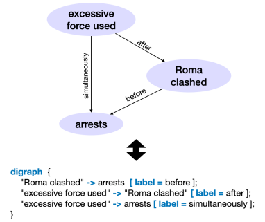
Figure 2: Temporal graph and the corresponding dot representation for the sentence: Roma clashed fiercely with the police, leading to arrests in which Roma activists said excessive force was used.

4 Model

The training data $\mathbf{X}$ for both Tasks 1 and 2 comprises of tuples $\{(\boldsymbol{x_{i}},\boldsymbol{y_{i}})\}_{i=1}^{N}$. For task 1 (node generation), $\boldsymbol{x_{i}}$ the concatenation of context, the source, node, and the relation. The target $\boldsymbol{y_{i}}$ consists of the tokens of the target event. For task 2 (graph generation), $\boldsymbol{x_{i}}$ is a document and $\boldsymbol{y_{i}}$ is the corresponding temporal graph represented in dot. We train a (separate) conditional language model to solve both the tasks. Specifically, given a training corpus of the form $\{(\boldsymbol{x_{i}},\boldsymbol{y_{i}})\}$, we aim to estimate the distribution $p_{\theta}(\boldsymbol{y_{i}}\mid\boldsymbol{x_{i}})$. Given a training example $(\boldsymbol{x_{i}},\boldsymbol{y_{i}})$ we set $\boldsymbol{u_{i}}=\boldsymbol{x_{i}}\|\boldsymbol{y_{i}}$. $p_{\theta}(\boldsymbol{u_{i}})$ can then be factorized as a sequence of auto-regressive conditional probabilities using the chain rule: $p_{\theta}(\boldsymbol{u_{i}})=\prod_{k=1}^{n}p(u_{i,k}|\boldsymbol{u_{i,<k}})$, where $u_{i,k}$ denotes the $k^{th}$ token of the $i^{th}$ sequence, and $\boldsymbol{u_{i,<k}}$ denotes the sequence of tokens $\{u_{1},u_{2},...,u_{k-1}\}$. Language models are typically trained by minimizing a cross-entropy loss $-\text{log}p_{\theta}(\boldsymbol{u_{i}})$ over each sequence $\boldsymbol{u_{i}}$ in $\mathbf{X}$. However, the cross-entropy loss captures the joint distribution $p_{\theta}(\boldsymbol{x_{i}},\boldsymbol{y_{i}})$, and is not aligned with our goal of learning conditional distribution $p_{\theta}(\boldsymbol{y_{i}}\mid\boldsymbol{x_{i}})$. To circumvent this, we train our model by masking the loss terms corresponding to the input $\boldsymbol{x_{i}}$, similar to Bosselut et al. (2019). Let $\boldsymbol{m_{i}}$ be a mask vector for each sequence $\boldsymbol{u_{i}}$, set to $0$ for positions corresponding to $\boldsymbol{x_{i}}$, and $1$ otherwise i.e. $m_{i,j}=1$ $\text{if }j>|\boldsymbol{x_{i}}|$, else 0. We combine the mask vector with our factorization of $p_{\theta}\left(\boldsymbol{u_{i}}\right)$ to formulate a masked language modeling loss $\mathcal{L}$, which is minimized over the training corpus $\mathbf{X}$ to estimate the optimal $\theta$:

$$\mathcal{L}(\mathbf{X})=-\sum_{i=1}^{|\mathbf{X}|}\sum_{j=1}^{|x_{i}|+|y_{i}|}m_{i,j}*\log\left(p_{\theta}\left(u_{i,j}|\boldsymbol{u_{i,<j}}\right)\right)$$

Note that the formulation of masked loss is opaque to the underlying architecture, and can be implemented with a simple change to the loss function. In practice, we use gpt-2 Radford et al. (2019) based on transformer architecture Vaswani et al. (2017) for our implementation. Having trained a $p_{\theta}$ for each task, we generate a node ($\boldsymbol{y}$) given a query ($\boldsymbol{x}$) (for Task 1), or a graph ($\boldsymbol{y}$) given a document ($\boldsymbol{x}$) (for Task 2) by drawing samples from the appropriate $p_{\theta}(\boldsymbol{y}\mid\boldsymbol{x})$ using nucleus sampling Holtzman et al. (2019). We provide more details of our training procedure and the architecture in the Appendix (C.1).

5 Experiments and Results

Method	Dataset	bleu	mtr	rg	acc
Seq2Seq	TG-Gen (-C)	20.20	14.62	31.95	19.68
Seq2Seq	TG-Gen	21.23	16.48	35.54	20.99
gpt-2	TG-Gen (-C)	36.60	25.11	43.07	35.07
gpt-2	TG-Gen	62.53	43.78	69.10	61.35
Seq2Seq	TB-Dense (-C)	11.55	9.23	21.87	10.06
Seq2Seq	TB-Dense	16.68	12.69	27.75	13.97
gpt-2	TB-Dense (-C)	22.35	15.04	27.73	20.81
gpt-2	TB-Dense	52.21	35.69	57.98	47.91

Table 3: Node Generation (task 1) results.

5.1 Evaluation Datasets

We evaluate our method on two different datasets: i) TG-Gen: Test split of synthetically created dataset (Section 3), and ii) TB-Dense: A mixed-domain corpus, with human-annotated temporal annotations. We create TB-Dense from the test splits of TimeBank-Dense Cassidy et al. (2014) by applying the same pre-processing operations as we did for TG-Gen. TB-Dense forms a very challenging dataset for our task because of domain mismatch; our system was trained on a corpus of terrorism-related events, whereas TB-Dense includes documents from a wide array of domains, forming a zero-shot evaluation scenario for our method.

5.2 Implementation Setup

gpt-2: We use gpt-2 medium (355M parameters) for our experiments with 24-layers, a hidden size of 1024, and 16 self-attention heads. We build on the implementation by Wolf et al. (2019), using the default hyperparameters and a block size input sequence length after tokenization) of 512. For optimization, we use AdamW Loshchilov and Hutter (2017) with a learning rate of 5e-5, a batch size of 1, and no learning rate scheduling. We also experimented with a block size of 300 and a batch size of 2. We found the results (presented in the appendix) to be worse, underscoring the importance of using a larger block size for generating larger outputs. We generate samples using nucleus sampling using $p=0.9$, and set maximum output length to be 500 for graph generation and 60 foe node generation. All of our experiments were done on a single Nvidia GeForce rtx 2080 Ti. The models were initialized with the pre-trained weights provided by Radford et al. (2019), and fine-tuned for five epochs, with a run-time of 48 hours/epoch for Task 1 and 52 hours/epoch for Task 2. We use the last checkpoint (i.e., at the end of fine-tuning) for all experiments. Despite the higher perplexity on the development set, we found the overall performance of the last checkpoint to be better.

We also experimented with gpt-2 without fine-tuning (i.e., by directly using pre-trained weights). The non-finetuned gpt-2 fared poorly for both the tasks across all the metrics, getting a bleu score of near 0 for Task 1. This dismal performance underscores the importance of fine-tuning on the end task for large-scale pre-trained language models.

Finally, we note that our method does not make any model-specific assumption, and can be used with any auto-regressive language model (i.e., a language model that generates a sequence of tokens from left-to-right). We use gpt-2 as a representative for large pre-trained language models.

Seq2Seq: We train a bi-directional lstm Hochreiter and Schmidhuber (1997) based sequence-to-sequence model Bahdanau et al. (2015) with global attention Luong et al. (2015) and a hidden size of 500 as a baseline to contrast with gpt-2. The token embeddings initialized using 300-dimensional pre-trained Glove Pennington et al. (2014).

5.3 Task 1: Node Generation

Paragraph: Mr. Grier, a former defensive lineman for the New York Giants who was ordained as a minister in 1986, testified on Dec. 9 that he had visited Mr. Simpson a month earlier

Table 4: An example of gpt-2 fixing the label given by caevo. Given a query event after “Mr. Grier visited”, caevo incorrectly extracts Mr. Grier ordained, whereas gpt-2 generates the correct event: Mr. Grier testified.

Metrics

Given a query $(C_{r},e_{q},r)$, with $C_{r}$ being the context (sentences containing events $e_{q},e_{t}$ and their neighboring sentences) and $e_{q}$ as the source event, Task 1 is to generate a target event $e_{t}$ such that $r(e_{q},e_{t})$. We format each query as “In the context of $C$, what happens $r$ $e_{q}$?”. We found formatting the query in natural language to be empirically better. Let $\hat{e_{t}}$ be the system generated event. We compare $e_{t}$ vs. $\hat{e_{t}}$ using bleu Papineni et al. (2002), meteor Denkowski and Lavie (2011), and rouge Lin (2004), and measure the accuracy (acc) as the fraction of examples where $e_{t}=\hat{e_{t}}$.

Results on TG-Gen The results are listed in Table 3. Unsurprisingly, gpt-2 achieves high scores across the metrics showing that it is highly effective in generating correct events. To test the generative capabilities of the models, we perform an ablation by removing the sentence containing the target event $e_{t}$ from $C_{r}$ (indicated with -C). Removal of context causes a drop in performance for both gpt-2 and Seq2Seq, showing that it is crucial for generating temporal events. However, gpt-2 obtains higher relative gains with context present, indicating that it uses its large architecture and pre-training to use the context more efficiently. gpt-2 also fares better as compared with Seq2Seq in terms of drop in performance for the out-of-domain TB-Dense dataset on metrics like accuracy ($-21\%$ vs. $-33\%$) and bleu ($-16\%$ vs. $-21\%$), indicating that pre-training makes helps gpt-2 in generalizing across the domains.

Human Evaluation To understand the nature of errors, we analyzed 100 randomly sampled incorrect generations. For 53% of the errors, gpt-2 generated a non-salient event which nevertheless had the correct temporal relation with the query. Interestingly, for 10% of the events, we found that gpt-2 fixed the label assigned by caevo (Table 4), i.e., $e_{t}$ was incorrect but $\hat{e_{t}}$ was correct.

5.4 Task 2: Graph Generation

	Dataset	bleu	mtr	rg	dot%
Seq2Seq	TG-Gen	4.79	15.03	45.95	86.93
gpt-2	TG-Gen	37.77	37.22	64.24	94.47
Seq2Seq	TB-Dense	2.61	12.76	28.36	89.31
gpt-2	TB-Dense	26.61	29.49	49.26	92.37

Table 5: Graph string metrics.

	Dataset	$v_{P}$	$v_{R}$	$v_{F_{1}}$	$e_{P}$	$e_{R}$	$e_{F_{1}}$
Seq2Seq	TG-Gen	36.84	24.89	28.11	9.65	4.29	4.70
gpt-2	TG-Gen	69.31	66.12	66.34	27.95	25.89	25.22
Seq2Seq	TB-Dense	24.86	15.25	17.99	4.7	0.14	0.24
caevo	TB-Dense	37.53	79.83	48.96	7.95	14.62	8.96
gpt-2	TB-Dense	45.96	48.44	44.97	8.74	8.89	7.96

Table 6: Graph semantic metrics.

Metrics Let $\mathbf{G_{i}}(\mathbf{V_{i}},\mathbf{E_{i}})$ and $\mathbf{\hat{G}_{i}}(\mathbf{\hat{V}_{i}},\mathbf{\hat{E}_{i}})$ be the true and the generated graphs for an example $i$ in the test corpus. Please recall that our proposed method generates a graph from a given document as a string in dot. Let $\boldsymbol{y_{i}}$ and $\boldsymbol{\hat{y_{i}}}$ be the string representations of the true and generated graphs. We evaluate our generated graphs using three types of metrics:

1. Graph string metrics: To compare $\boldsymbol{y_{i}}$ vs. $\boldsymbol{\hat{y_{i}}}$, we use bleu, meteor, and rouge, and also measure parse accuracy (dot%) as the % of generated graphs $\boldsymbol{\hat{y_{i}}}$ which are valid dot files.

2. Graph structure metrics To compare the structures of the graphs $\mathbf{G_{i}}$ vs. $\mathbf{\hat{G}_{i}}$, we use i) Graph edit distance (ged) Abu-Aisheh et al. (2015) - the minimum numbers of edits required to transform the predicted graph to the true graph by addition/removal of an edge/node; ii) Graph isomorphism (iso) Cordella et al. (2001) - a binary measure set to $1$ if the graphs are isomorphic (without considering the node or edge attributes); iii) The average graph size $(|\mathbf{V_{i}}|,|\mathbf{E_{i}}|,|\mathbf{\hat{V}_{i}}|,|\mathbf{\hat{E}_{i}}|)$ and the average degree ($\text{d}(\mathbf{V})$).

3. Graph semantic metrics: We evaluate the node sets ($\mathbf{V_{i}}$ vs. $\mathbf{\hat{V}_{i}}$) and the edge sets ($\mathbf{E_{i}}$ vs. $\mathbf{\hat{E}_{i}}$) to compare the semantics of the true and generated graphs. For every example $i$, we calculate node-set precision, recall, and $F_{1}$ score, and average them over the test set to obtain node precision ($v_{P}$), recall ($v_{R}$), and $F_{1}$ ($v_{F}$). We evaluate the predicted edge set using temporal awareness UzZaman and Allen (2012); UzZaman et al. (2013). For an example $i$, we calculate $e_{P}^{i}=\frac{|\mathbf{\hat{E}_{i}}^{-}\cap\mathbf{E_{i}}^{+}|}{|\mathbf{\hat{E}_{i}}^{-}|},e_{R}^{i}=\frac{|\mathbf{\hat{E}_{i}}^{+}\cap\mathbf{E_{i}}^{-}|}{|\mathbf{E_{i}}^{-}|}$ where symbol $+$ denotes the temporal transitive closure Allen (1983) of the edge set. Similarly, $-$ indicates the reduced edge set, obtained by removing all the edges that can be inferred from other edges transitively. The $F_{1}$ score $e_{F_{1}}^{i}$ is the harmonic mean of $e_{P}^{i}$ and $e_{R}^{i}$, and these metrics are averaged over the test set to obtain the temporal awareness precision ($e_{P}$), recall ($e_{R}$), and $F_{1}$ score ($e_{F_{1}}$). Intuitively, the node metrics judge the quality of generated events in the graph, and the edge metrics evaluate the corresponding temporal relations.

Results

Tables 5, 7, and 6 present results for graph generation, and we discuss them next.

	Dataset	$|\mathbf{V}|$	$|\mathbf{E}|$	$\textit{d}(\mathbf{V})$	ged $\downarrow$	iso $\uparrow$
True	TG-Gen	4.15	5.47	1.54	0	100
Seq2Seq	TG-Gen	2.24	2.23	1.12	6.09	32.49
gpt-2	TG-Gen	3.81	4.60	1.40	2.62	41.66
True	TB-Dense	4.39	6.12	2.02	0	100
Seq2Seq	TB-Dense	2.21	2.20	1.11	6.22	23.08
caevo	TB-Dense	10.73	17.68	2.76	18.68	11.11
gpt-2	TB-Dense	3.72	4.65	1.75	4.05	24.00

Table 7: Graph structure metrics.

gpt-2 vs. Seq2Seq

gpt-2 outperforms Seq2Seq on all the metrics by a large margin in both fine-tuned (TG-Gen) and zero-shot settings (TB-Dense). gpt-2 generated graphs are closer to the true graphs in size and topology, as shown by lower edit distance and a higher rate of isomorphism in Table 7. Both the systems achieve high parsing rates (dot %), with gpt-2 generating valid dot files 94.6% of the time. The high parsing rates are expected, as even simpler architectures like vanilla RNNs have been shown to generate syntactically valid complex structures like LaTeXdocuments with ease Karpathy (2015).

gpt-2 vs. caevo

We compare the graphs generated by gpt-2 with those extracted by caevo Chambers et al. (2014) from the TB-Dense documents. We remove all the vague edges and the light verbs from the output of caevo for a fair comparison. Please recall that caevo is the tool we used for creating the training data for our method. Further, caevo was trained using TB-Dense, while gpt-2 was not. Thus, caevo forms an upper bound over the performance of gpt-2. The results in Tables 6 and 7 show that despite these challenges, gpt-2 performs strongly across a wide range of metrics, including ged, iso, and temporal awareness. Comparing the node-set metrics, we see that gpt-2 leads caevo by over eight precision points ($v_{P}$), but loses on recall ($v_{R}$) as caevo extracts nearly every verb in the document as a potential event. On temporal awareness (edge-metrics), gpt-2 outperforms both caevo and Seq2Seq in terms of average precision score $e_{P}$ and achieves a competitive $e_{F_{1}}$ score. These results have an important implication: they show that our method can best or match a pipeline of specialized systems given reasonable amounts of training data for temporal graph extraction. caevo involves several sub-modules to perform part-of-speech tagging, dependency parsing, event extraction, and several statistical and rule-based systems for temporal extraction. In contrast, our method involves no hand-curated features, is trained end-to-end (single gpt-2), and can be easily scaled to new datasets.

Top 10 Verbs: found, killed, began, called, want, took, came, used, trying, asked

Randomly Sampled Verbs: shooting, caused, accused, took, conceived, visit, vowing, play, withdraw, seems

Table 8: Verbs in gpt-2 generated graphs.

Node extraction and Edge Extraction

The node-set metrics in Table 6 shows that gpt-2 avoids generating noisy events (high $P$), and extracts salient events (high $R$). This is confirmed by manual analysis, done by randomly sampling 100 graphs from the gpt-2 generated graphs and isolating the main verb in each node (Table 8). We provide several examples of generated graphs in the Appendix. We note from Table 6 that the relative difference between the $e_{F_{1}}$ scores for gpt-2 and Seq2Seq (25.22 vs. 4.70) is larger than the relative difference between their $v_{F_{1}}$ scores (66.34 vs. 28.11), showing that edge-extraction is the more challenging task which allows gpt-2 to take full advantage of its powerful architecture. We also observe that edge extraction ($e_{F_{1}}$) is highly sensitive to node extraction ($v_{F_{1}}$); for gpt-2, a 27% drop in $v_{F_{1}}$ (66.34 on TG-Gen vs. 44.97 on TB-Dense) causes a 68% drop in $e_{F_{1}}$ (25.22 on TG-Gen vs. 7.96 on TB-Dense). As each node is connected to multiple edges on average (Table 7), missing a node during the generation process might lead to multiple edges being omitted, thus affecting edge extraction metrics disproportionately.

Query ($C,e_{q},r$)	$e_{t}$	Explanation
The suspected car bombings…turning busy streets…Which event happened before the suspected car bombings?	many cars drove	Plausible: The passage mentions busy streets and car bombing.
He…charged…killed one person. Which event happened after he was charged?	He was acquitted	Somewhat plausible: An acquittal is a possible outcome of a trial.

Table 9: Sample open-ended questions and the answers $e_{t}$ generated by our system. Note that the answers generated by our system $e_{t}$ are complete event phrases (not just verbs).

5.5 Answering for Open-ended Questions

A benefit of our approach of using a pre-trained language model is that it can be used to generate an answer for open-ended temporal questions. Recently, Ning et al. (2020) introduced Torque, a temporal reading-comprehension dataset. Several questions in Torque have no answers, as they concern a time scope not covered by the passage (the question is about events not mentioned in the passage). We test the ability of our system for generating plausible answers for such questions out of the box (i.e., without training on Torque). Given a (passage, question) pair, we create a query $(C,e_{q},r)$, where $C$ is the passage, and $e_{q}$ and $r$ are the query event and temporal relation in the question. We then use our gpt-2 based model for node-generation trained without context and generate an answer $e_{t}$ for the given query. A human-judge rated the answers generated for 100 such questions for plausibility, rating each answer as being plausible, somewhat plausible, or incorrect. For each answer rated as either plausible or somewhat plausible, the human-judge wrote a short explanation to provide a rationale for the plausibility of the generated event. Out of the 100 questions, the human-judge rated 22 of the generated answers as plausible and ten as somewhat plausible, showing the promise of our method on this challenging task (Table 9).

6 Conclusion and Future Work

Current methods for generating event-level temporal graphs are developed with relatively small amounts of hand-labeled data. On the other hand, the possibility of using pre-trained language models for this task has not received sufficient attention. This paper addresses this open challenge by first developing a data generation pipeline that uses existing ie/nlp/clustering techniques for automated acquisition of a large corpus of document-graph pairs, and by proposing a new formulation of the graph generation task as a sequence-to-sequence mapping task, allowing us to leverage and fine-tune pre-trained language models. Our experiments strongly support the effectiveness of the proposed approach, which significantly outperforms strong baselines. We plan to explore techniques for adapting large-scale language models on unseen domains and at multiple granularity levels in the future.

Appendix A Learning Event Communities Using Community Detection

In this section, we provide the details on the community detection algorithm used by our method. We define the temporal event communities to be a division of the temporal graph $\mathbf{G}(\mathbf{V},\mathbf{E})$ into sub-graphs $\mathbf{G_{1}}(\mathbf{V_{1}},\mathbf{E_{1}}),\mathbf{G_{2}}(\mathbf{V_{2}},\mathbf{E_{2}}),...,\mathbf{G_{k}}(\mathbf{V_{k}},\mathbf{E_{k}})$ such that the events in a community (sub-graph) $\mathbf{G_{i}}$ are more co-referential to each other as opposed to the other events in the temporal graph. We use the undirected link between two events $e_{j},e_{i}$ as a proxy for them being co-referential, and learn temporal event communities utilizing the concept of modularity, first introduced by Newman and Girvan (2004).

Formally, let $\mathbf{A}$ be the undirected adjacency matrix for a temporal graph $\mathbf{G}(\mathbf{V},\mathbf{E})$ such that $\mathbf{A}(e_{i},e_{j})=1$ if $e_{i}$ and $e_{j}$ are connected by a temporal relation, and 0 otherwise. Further, let $\delta(e_{i},e_{j})=1$ if events $e_{i},e_{j}$ belong to the same temporal community, and $0$ otherwise. For a given $\delta$, we denote the fraction of the edges that exist between events that belong to the same communities by $f_{same}=\frac{\sum_{e_{i},e_{j}\in\mathbf{E}}\mathbf{A}(e_{i},e_{j})\delta(e_{i},e_{j})}{2|\mathbf{E}|}$. Where the $2|\mathbf{E}|$ in the denominator is due to the fact that $\mathbf{A}$ treats $\mathbf{G}$ as an undirected graph. Let the popularity $p$ of an event $e_{i}$ be the number of events that are linked to it i.e. $p(e_{i})=\sum_{e_{j}\in\mathbf{E}}\mathbf{A}(e_{i},e_{j})$. The probability of randomly picking an event $e_{i}$ when sampled by popularity is $\frac{p(e_{i})}{\sum_{e_{j}\in\mathbf{E}}p(e_{i})}=\frac{p(e_{i})}{2|\mathbf{E}|}$. Thus, if edges are created randomly by sampling nodes by popularity $p$ of the nodes, the fraction of edges within the communities, $f_{random}$, is given by

$$f_{random} =\frac{\sum_{e_{i},e_{j}\in\mathbf{E}}p(e_{i})p(e_{j})\delta(e_{i},e_{j})}{2|\mathbf{E}|*2|\mathbf{E}|}$$

Finally, defining modularity, $Q$, to be $f_{same}-f_{random}$:

$$Q =\frac{1}{2|\mathbf{E}|}*\sum_{e_{i},e_{j}\in\mathbf{E}}\mathbf{A}(e_{i},e_{j})-\frac{p(e_{i})p(e_{j})\delta(e_{i},e_{j})}{2|\mathbf{E}|}$$

We want to learn community assignments $\delta$ that maximize $Q$. A high $Q$ would promote $f_{same}>f_{random}$ and thereby encourage highly inter-connected event communities. Calculating such $\delta$ directly is not tractable, since the complexity of such an operation would be at least exponential in the number of events Newman (2004). We use the fast implementation provided by Clauset et al. (2004) for calculating event communities iteratively. The algorithm converges at $Q~{}0.3$. We use a similar approximation at test time: given a document $D$, we first break it down into sub-documents using caevo and then feed each sub-document to our method.

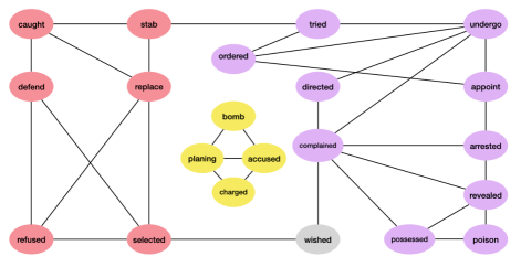
Figure 3: Event temporal graph and the extracted communities for a sample document. Each community is shown in different color. The singleton nodes (gray) are dropped. The nodes are only annotated with the verbs for brevity. The edge labels and directions are not used for community detection.

Appendix B Using a smaller block size

We found that the performance drops when using a block size of 300 and batch size of 2. Table 10 presents the results.

bleu	mtr	rg	dot%
25.01	27.95	60.99	91.71

$v_{P}$	$v_{R}$	$v_{F_{1}}$	$e_{P}$	$e_{R}$	$e_{F_{1}}$
70.31	64.75	65.68	29.43	24.83	24.27

Table 10: Results for TG-Gen using a block size of 300 and a block size of 2.

Appendix C Masked Language Modeling Using Transformers

In this section, we expand on the design of the transformer blocks. For ease of reference, we re-iterate our training methodology. We train a (separate) conditional language model to solve both the tasks. Specifically, given a training corpus of the form $\{(\boldsymbol{x_{i}},\boldsymbol{y_{i}})\}$, we aim to estimate the distribution $p_{\theta}(\boldsymbol{y_{i}}\mid\boldsymbol{x_{i}})$. Given a training example $(\boldsymbol{x_{i}},\boldsymbol{y_{i}})$ we set $\boldsymbol{u_{i}}=\boldsymbol{x_{i}}\|\boldsymbol{y_{i}}$. $p_{\theta}(\boldsymbol{u_{i}})$ can then be factorized as a sequence of auto-regressive conditional probabilities using the chain rule: $p_{\theta}(\boldsymbol{u_{i}})=\prod_{k=1}^{n}p(u_{i,k}|\boldsymbol{u_{i,<k}})$, where $u_{i,k}$ denotes the $k^{th}$ token of the $i^{th}$ sequence, and $\boldsymbol{u_{i,<k}}$ denotes the sequence of tokens $\{u_{1},u_{2},...,u_{k-1}\}$. Language models are typically trained by minimizing a cross-entropy loss $-\text{log}p_{\theta}(\boldsymbol{u_{i}})$ over each sequence $\boldsymbol{u_{i}}$ in $\mathbf{X}$. However, the cross-entropy loss captures the joint distribution $p_{\theta}(\boldsymbol{x_{i}},\boldsymbol{y_{i}})$, and is not aligned with our goal of learning conditional distribution $p_{\theta}(\boldsymbol{y_{i}}|\boldsymbol{x_{i}})$. To circumvent this, we train our model by masking the loss terms corresponding to the input $\boldsymbol{x_{i}}$, similar to Bosselut et al. (2019). Let $\boldsymbol{m_{i}}$ be a mask vector for each sequence $\boldsymbol{u_{i}}$, set to $0$ for positions corresponding to $\boldsymbol{x_{i}}$, and $1$ otherwise i.e. $m_{i,j}=1$ $\text{if }j>|\boldsymbol{x_{i}}|$, else 0. We combine the mask vector with our factorization of $p_{\theta}(\boldsymbol{u_{i}})$ to formulate a masked language modeling loss, which is minimized over the training corpus $\mathbf{X}$ to estimate the optimal $\theta$:

$$\mathcal{L}_{\textit{masked}}(\mathbf{X})=-\sum_{i=1}^{|\mathbf{X}|}\sum_{j=1}^{|x_{i}|+|y_{i}|}m_{i,j}*\text{log}(p_{\theta}(u_{i,j}|\boldsymbol{u_{i,<j}}))$$

Note that the formulation of masked loss is opaque to the underlying architecture, and can be implemented with a simple change to the loss function. Intuitively, the model is optimized for only the output sequence $y_{i}$.

C.1 Adapting gpt-2 for Masked Language Modeling

In practice, we use gpt-2 Radford et al. (2019) based on transformer architecture Vaswani et al. (2017) for our implementation. An input sequence $\boldsymbol{u_{i}}$ of length $n$ is first embedded to a continuous representation denoted by $\boldsymbol{u_{i}}^{(0)}\in\mathbb{R}^{nd}$. $\boldsymbol{u_{i}}^{(0)}$ is then passed through a series of $L$ transformer blocks to obtain the output sequence $\boldsymbol{u_{i}}^{(L)}\in\mathbb{R}^{nh}$. Each transformer block Vaswani et al. (2017) consists of two operations: an auto-regressive version of the multiheaded self-attention Vaswani et al. (2017) operation (AutoRegMultiHead) followed by a feed-forward operation (FFN). Each of these operations is surrounded by a residual connection He et al. (2016) and followed by a layer normalization Ba et al. (2016) operation. Denoting by $\boldsymbol{u}^{(l-1)}$ the input to the $l^{th}$ transformer block , the operations are in a transformer block are defined as follows:

$$\tilde{\boldsymbol{u}}_{attn}^{l} =\textit{AutoRegMultiHead}(\boldsymbol{u}^{(l-1)})$$

$$\boldsymbol{u}_{att}^{(l)} =\textit{LayerNorm}(\tilde{\boldsymbol{u}}_{att}^{(l)}+\boldsymbol{u}^{(l-1)})$$

$$\tilde{\boldsymbol{u}}_{ffn}^{(l)} =\textit{FFN}(\boldsymbol{u}_{att}^{(l)})$$

$$\boldsymbol{u}^{(l)} =\textit{LayerNorm}(\tilde{\boldsymbol{u}}_{ffn}^{(l)}+\boldsymbol{u}_{att}^{(l)})$$

Where AutoRegMultiHead is an auto-regressive version of the multiheaded self-attention Vaswani et al. (2017) that restricts the attention to the sequence seen so far (in accordance with the chain rule), and FFN is a feed-forward network (mlp). After obtaining $\boldsymbol{u_{i}}^{(L)}$, we set $p_{\phi}(\boldsymbol{u_{i}})=\text{softmax}(\boldsymbol{u_{i}}^{(L)}*\mathbf{W}_{e})$, where $\mathbf{W}_{e}\in\mathbb{R}^{h|V|}$ ($|V|$ is the size of the vocabulary). Finally, we calculate the masked loss as $\mathcal{L}(\boldsymbol{u_{i}})=\boldsymbol{m_{i}}^{T}\odot\text{log}(p_{\phi}(\boldsymbol{u_{i}}))$, and the optimal $\phi$ is obtained by minimizing $\mathcal{L}_{\textit{masked}}(\mathbf{X})=-\sum_{i=1}^{|\mathbf{X}|}\mathcal{L}(\boldsymbol{u_{i}})$.

Appendix D Dataset Statistics

Tables 11,  12, and 13 list various statistics calculated from the source data.

Descriptor	#Articles
terrorism	40909
murders and attempted murders	25169
united states international relations	17761
united states armament and defense	16785
airlines and airplanes	16103
world trade center (nyc)	15145
demonstrations and riots	14477
hijacking	14472
politics and government	6270
bombs and explosives	5607

Table 11: Top Descriptors for the filtered Dataset. Note that each article is typically assigned more than one descriptor.

Event verb	Raw frequency	% Frequency
said	647685	9.60
say	57667	0.86
had	47320	0.70
killed	43369	0.64
told	42983	0.64
found	41733	0.62
made	40544	0.60
war	35257	0.52
get	30726	0.46
make	29407	0.44

Table 12: Most frequent events extracted by caevo.

Relation	Raw Frequency	% Frequency
before	2436201	54.51
after	1772071	39.65
is included	131052	2.93
simultaneous	112509	2.52
includes	17465	0.39

Table 13: Relation Frequence in our Corpus

Relation	Frequency
before	98715
after	68582
is included	6179
simultaneous	6209
includes	285

Table 14: Edges in Generated Graphs: Top

Appendix E Examples

Figures 4-9 show randomly picked examples from the test corpus. Each figure shows the text, the corresponding true graph, and the graph predicted by gpt-2.

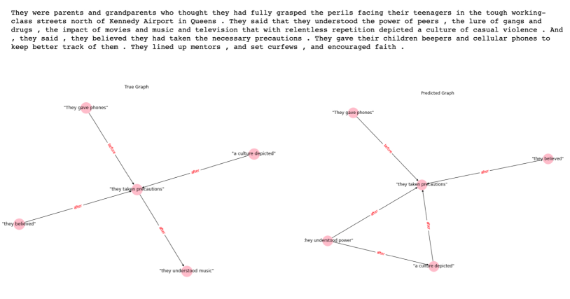
Figure 4:

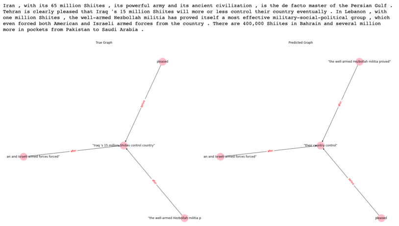
Figure 5:

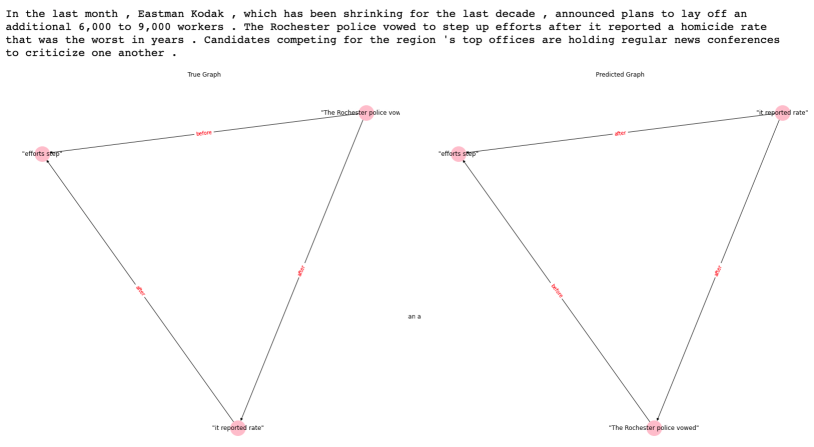
Figure 6:

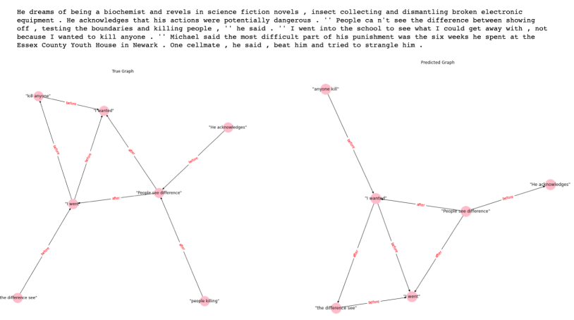
Figure 7:

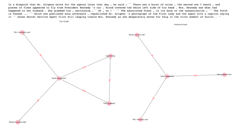
Figure 8:

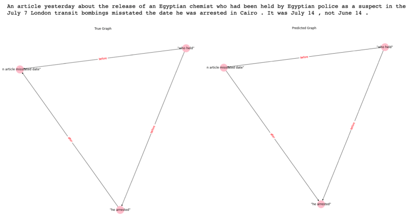
Figure 9:

References

- Abu-Aisheh et al. (2015) Zeina Abu-Aisheh, Romain Raveaux, Jean-Yves Ramel, and Patrick Martineau. 2015. An exact graph edit distance algorithm for solving pattern recognition problems. In An exact graph edit distance algorithm for solving pattern recognition problems.
- Allen (1983) James F Allen. 1983. Maintaining knowledge about temporal intervals. Communications of the ACM, 26(11):832–843.
- Ba et al. (2016) Jimmy Lei Ba, Jamie Ryan Kiros, and Geoffrey E Hinton. 2016. Layer normalization. arXiv preprint arXiv:1607.06450.
- Bahdanau et al. (2015) Dzmitry Bahdanau, Kyunghyun Cho, and Yoshua Bengio. 2015. Neural machine translation by jointly learning to align and translate. In 3rd International Conference on Learning Representations, ICLR 2015.
- Ballesteros et al. (2020) Miguel Ballesteros, Rishita Anubhai, Shuai Wang, Nima Pourdamghani, Yogarshi Vyas, Jie Ma, Parminder Bhatia, Kathleen McKeown, and Yaser Al-Onaizan. 2020. Severing the edge between before and after: Neural architectures for temporal ordering of events. arXiv preprint arXiv:2004.04295.
- Bosselut et al. (2019) Antoine Bosselut, Hannah Rashkin, Maarten Sap, Chaitanya Malaviya, Asli Çelikyilmaz, and Yejin Choi. 2019. Comet: Commonsense transformers for automatic knowledge graph construction. In ACL.
- Brown et al. (2020) Tom B Brown, Benjamin Mann, Nick Ryder, Melanie Subbiah, Jared Kaplan, Prafulla Dhariwal, Arvind Neelakantan, Pranav Shyam, Girish Sastry, Amanda Askell, et al. 2020. Language models are few-shot learners. arXiv preprint arXiv:2005.14165.
- Budzianowski and Vulić (2019) Paweł Budzianowski and Ivan Vulić. 2019. Hello, it’s gpt-2–how can i help you? towards the use of pretrained language models for task-oriented dialogue systems. arXiv preprint arXiv:1907.05774.
- Cassidy et al. (2014) Taylor Cassidy, Bill McDowell, Nathanel Chambers, and Steven Bethard. 2014. An annotation framework for dense event ordering. Technical report, CARNEGIE-MELLON UNIV PITTSBURGH PA.
- Chambers et al. (2014) Nathanael Chambers, Taylor Cassidy, Bill McDowell, and Steven Bethard. 2014. Dense event ordering with a multi-pass architecture. Transactions of the Association for Computational Linguistics, 2:273–284.
- Chambers and Jurafsky (2008) Nathanael Chambers and Dan Jurafsky. 2008. Unsupervised learning of narrative event chains. In Proceedings of ACL-08: HLT, pages 789–797.
- Chambers and Jurafsky (2009) Nathanael Chambers and Dan Jurafsky. 2009. Unsupervised learning of narrative schemas and their participants. In Proceedings of the Joint Conference of the 47th Annual Meeting of the ACL and the 4th International Joint Conference on Natural Language Processing of the AFNLP, pages 602–610.
- Cheng and Miyao (2017) Fei Cheng and Yusuke Miyao. 2017. Classifying temporal relations by bidirectional lstm over dependency paths. In Proceedings of the 55th Annual Meeting of the Association for Computational Linguistics (Volume 2: Short Papers), pages 1–6.
- Clauset et al. (2004) Aaron Clauset, Mark EJ Newman, and Cristopher Moore. 2004. Finding community structure in very large networks. Physical review E, 70(6):066111.
- Cordella et al. (2001) Luigi Pietro Cordella, Pasquale Foggia, Carlo Sansone, and Mario Vento. 2001. An improved algorithm for matching large graphs. In 3rd IAPR-TC15 workshop on graph-based representations in pattern recognition, pages 149–159.
- Denkowski and Lavie (2011) Michael Denkowski and Alon Lavie. 2011. Meteor 1.3: Automatic metric for reliable optimization and evaluation of machine translation systems. In Proceedings of the sixth workshop on statistical machine translation, pages 85–91. Association for Computational Linguistics.
- Duran et al. (2007) Nicholas D Duran, Philip M McCarthy, Art C Graesser, and Danielle S McNamara. 2007. Using temporal cohesion to predict temporal coherence in narrative and expository texts. Behavior Research Methods, 39(2):212–223.
- Evers-Vermeul et al. (2017) Jacqueline Evers-Vermeul, Jet Hoek, and Merel CJ Scholman. 2017. On temporality in discourse annotation: Theoretical and practical considerations. Dialogue & Discourse, 8(2):1–20.
- Gansner et al. (2006) Emden Gansner, Eleftherios Koutsofios, and Stephen North. 2006. Drawing graphs with dot.
- Goyal and Durrett (2019) Tanya Goyal and Greg Durrett. 2019. Embedding time expressions for deep temporal ordering models. In Proceedings of the 57th Annual Meeting of the Association for Computational Linguistics, pages 4400–4406, Florence, Italy. Association for Computational Linguistics.
- Hagberg et al. (2008) Aric A. Hagberg, Daniel A. Schult, and Pieter J. Swart. 2008. Exploring network structure, dynamics, and function using networkx. In Proceedings of the 7th Python in Science Conference, pages 11 – 15, Pasadena, CA USA.
- Han et al. (2019) Rujun Han, I-Hung Hsu, Mu Yang, Aram Galstyan, Ralph Weischedel, and Nanyun Peng. 2019. Deep structured neural network for event temporal relation extraction. In Proceedings of the 23rd Conference on Computational Natural Language Learning (CoNLL), pages 666–106.
- He et al. (2016) Kaiming He, Xiangyu Zhang, Shaoqing Ren, and Jian Sun. 2016. Deep residual learning for image recognition. In Proceedings of the IEEE conference on computer vision and pattern recognition, pages 770–778.
- Hochreiter and Schmidhuber (1997) Sepp Hochreiter and Jürgen Schmidhuber. 1997. Long short-term memory. Neural computation, 9(8):1735–1780.
- Holtzman et al. (2019) Ari Holtzman, Jan Buys, Li Du, Maxwell Forbes, and Yejin Choi. 2019. The curious case of neural text degeneration. arXiv preprint arXiv:1904.09751.
- Karpathy (2015) Andrej Karpathy. 2015. The unreasonable effectiveness of recurrent neural networks. Andrej Karpathy blog, 21:23.
- Lin et al. (2016) Chen Lin, Dmitriy Dligach, Timothy A Miller, Steven Bethard, and Guergana K Savova. 2016. Multilayered temporal modeling for the clinical domain. Journal of the American Medical Informatics Association, 23(2):387–395.
- Lin (2004) Chin-Yew Lin. 2004. Rouge: A package for automatic evaluation of summaries. In Text summarization branches out, pages 74–81.
- Ling and Weld (2010) Xiao Ling and Daniel S Weld. 2010. Temporal information extraction. In AAAI, volume 10, pages 1385–1390.
- Liu et al. (2018) Zhengzhong Liu, Chenyan Xiong, Teruko Mitamura, and Eduard Hovy. 2018. Automatic event salience identification. arXiv preprint arXiv:1809.00647.
- Loshchilov and Hutter (2017) Ilya Loshchilov and Frank Hutter. 2017. Decoupled weight decay regularization. arXiv preprint arXiv:1711.05101.
- Luong et al. (2015) Minh-Thang Luong, Hieu Pham, and Christopher D Manning. 2015. Effective approaches to attention-based neural machine translation. In Proceedings of the 2015 Conference on Empirical Methods in Natural Language Processing, pages 1412–1421.
- Madaan et al. (2020) Aman Madaan, Dheeraj Rajagopal, Yiming Yang, Abhilasha Ravichander, Eduard Hovy, and Shrimai Prabhumoye. 2020. Eigen: Event influence generation using pre-trained language models. arXiv preprint arXiv:2010.11764.
- Makkonen et al. (2003) Juha Makkonen, Helena Ahonen-Myka, and Marko Salmenkivi. 2003. Topic detection and tracking with spatio-temporal evidence. In European Conference on Information Retrieval, pages 251–265. Springer.
- Newman (2004) Mark EJ Newman. 2004. Fast algorithm for detecting community structure in networks. Physical review E, 69(6):066133.
- Newman and Girvan (2004) Mark EJ Newman and Michelle Girvan. 2004. Finding and evaluating community structure in networks. Physical review E, 69(2):026113.
- Ning et al. (2019a) Qiang Ning, Zhili Feng, and Dan Roth. 2019a. A structured learning approach to temporal relation extraction. arXiv preprint arXiv:1906.04943.
- Ning et al. (2019b) Qiang Ning, Sanjay Subramanian, and Dan Roth. 2019b. An improved neural baseline for temporal relation extraction. arXiv preprint arXiv:1909.00429.
- Ning et al. (2020) Qiang Ning, Hao Wu, Rujun Han, Nanyun Peng, Matt Gardner, and Dan Roth. 2020. Torque: A reading comprehension dataset of temporal ordering questions. arXiv preprint arXiv:2005.00242.
- Ning et al. (2018) Qiang Ning, Ben Zhou, Zhili Feng, Haoruo Peng, and Dan Roth. 2018. Cogcomptime: A tool for understanding time in natural language. In Proceedings of the 2018 Conference on Empirical Methods in Natural Language Processing: System Demonstrations, pages 72–77.
- Papineni et al. (2002) Kishore Papineni, Salim Roukos, Todd Ward, and Wei-Jing Zhu. 2002. Bleu: a method for automatic evaluation of machine translation. In Proceedings of the 40th annual meeting on association for computational linguistics, pages 311–318. Association for Computational Linguistics.
- Pennington et al. (2014) Jeffrey Pennington, Richard Socher, and Christopher D. Manning. 2014. Glove: Global vectors for word representation. In Empirical Methods in Natural Language Processing (EMNLP), pages 1532–1543.
- Radford et al. (2018) Alec Radford, Karthik Narasimhan, Tim Salimans, and Ilya Sutskever. 2018. Improving language understanding by generative pre-training. URL https://s3-us-west-2. amazonaws. com/openai-assets/researchcovers/languageunsupervised/language understanding paper. pdf.
- Radford et al. (2019) Alec Radford, Jeffrey Wu, Rewon Child, David Luan, Dario Amodei, and Ilya Sutskever. 2019. Language models are unsupervised multitask learners. OpenAI Blog, 1(8):9.
- Raffel et al. (2019) Colin Raffel, Noam Shazeer, Adam Roberts, Katherine Lee, Sharan Narang, Michael Matena, Yanqi Zhou, Wei Li, and Peter J Liu. 2019. Exploring the limits of transfer learning with a unified text-to-text transformer. arXiv preprint arXiv:1910.10683.
- Rajagopal et al. (2021) Dheeraj Rajagopal, Aman Madaan, Niket Tandon, Yiming Yang, Shrimai Prabhumoye, Abhilasha Ravichander, Peter Clark, and Eduard Hovy. 2021. Curie: An iterative querying approach for reasoning about situations.
- Recasens et al. (2010) Marta Recasens, Eduard H Hovy, and Maria Antònia Martí. 2010. A typology of near-identity relations for coreference (nident). In LREC.
- Sap et al. (2019) Maarten Sap, Ronan Le Bras, Emily Allaway, Chandra Bhagavatula, Nicholas Lourie, Hannah Rashkin, Brendan Roof, Noah A Smith, and Yejin Choi. 2019. Atomic: An atlas of machine commonsense for if-then reasoning. In Proceedings of the AAAI Conference on Artificial Intelligence, volume 33, pages 3027–3035.
- Sharma et al. (2017) Shikhar Sharma, Layla El Asri, Hannes Schulz, and Jeremie Zumer. 2017. Relevance of unsupervised metrics in task-oriented dialogue for evaluating natural language generation. CoRR, abs/1706.09799.
- Speer et al. (2017) Robyn Speer, Joshua Chin, and Catherine Havasi. 2017. Conceptnet 5.5: An open multilingual graph of general knowledge. In Thirty-First AAAI Conference on Artificial Intelligence.
- Sutskever et al. (2014) Ilya Sutskever, Oriol Vinyals, and Quoc V Le. 2014. Sequence to sequence learning with neural networks. In Advances in neural information processing systems, pages 3104–3112.
- UzZaman and Allen (2012) Naushad UzZaman and James F Allen. 2012. Interpreting the temporal aspects of language. Citeseer.
- UzZaman et al. (2013) Naushad UzZaman, Hector Llorens, Leon Derczynski, James Allen, Marc Verhagen, and James Pustejovsky. 2013. Semeval-2013 task 1: Tempeval-3: Evaluating time expressions, events, and temporal relations. In Second Joint Conference on Lexical and Computational Semantics (* SEM), Volume 2: Proceedings of the Seventh International Workshop on Semantic Evaluation (SemEval 2013), pages 1–9.
- Vashishtha et al. (2019) Siddharth Vashishtha, Benjamin Van Durme, and Aaron Steven White. 2019. Fine-grained temporal relation extraction. In Proceedings of the 57th Annual Meeting of the Association for Computational Linguistics, pages 2906–2919, Florence, Italy. Association for Computational Linguistics.
- Vaswani et al. (2017) Ashish Vaswani, Noam Shazeer, Niki Parmar, Jakob Uszkoreit, Llion Jones, Aidan N Gomez, Łukasz Kaiser, and Illia Polosukhin. 2017. Attention is all you need. In Advances in neural information processing systems, pages 5998–6008.
- Wolf et al. (2019) Thomas Wolf, L Debut, V Sanh, J Chaumond, C Delangue, A Moi, P Cistac, T Rault, R Louf, M Funtowicz, et al. 2019. Huggingface’s transformers: State-of-the-art natural language processing. ArXiv, abs/1910.03771.
- You et al. (2018) Jiaxuan You, Rex Ying, Xiang Ren, William L Hamilton, and Jure Leskovec. 2018. Graphrnn: Generating realistic graphs with deep auto-regressive models. arXiv preprint arXiv:1802.08773.