Deep Low-Shot Learning for Biological Image Classification and Visualization from Limited Training Samples
Abstract
Predictive modeling is useful but very challenging in biological image analysis due to the high cost of obtaining and labeling training data. For example, in the study of gene interaction and regulation in Drosophila embryogenesis, the analysis is most biologically meaningful when in situ hybridization (ISH) gene expression pattern images from the same developmental stage are compared. However, labeling training data with precise stages is very time-consuming even for developmental biologists. Thus, a critical challenge is how to build accurate computational models for precise developmental stage classification from limited training samples. In addition, identification and visualization of developmental landmarks are required to enable biologists to interpret prediction results and calibrate models. To address these challenges, we propose a deep two-step low-shot learning framework to accurately classify ISH images using limited training images. Specifically, to enable accurate model training on limited training samples, we formulate the task as a deep low-shot learning problem and develop a novel two-step learning approach, including data-level learning and feature-level learning. We use a deep residual network as our base model and achieve improved performance in the precise stage prediction task of ISH images. Furthermore, the deep model can be interpreted by computing saliency maps, which consist of pixel-wise contributions of an image to its prediction result. In our task, saliency maps are used to assist the identification and visualization of developmental landmarks. Our experimental results show that the proposed model can not only make accurate predictions, but also yield biologically meaningful interpretations. We anticipate our methods to be easily generalizable to other biological image classification tasks with small training datasets. Our open-source code is available at https://github.com/divelab/lsl-fly.
Index Terms:
Biological image classification; limited training samples; Drosophila ISH images; deep two-step low-shot learning; model interpretation and visualizationI Introduction
In biological image analysis tasks, annotation of training images usually requires specific domain knowledge and thus is commonly performed by expert biologists. This manual practice and the incurred cost limit the number of labeled training samples. Therefore, a recurring theme in biological image analysis is how to enable efficient and accurate model training from limited labeled training samples [1]. For example, comparative analysis of in situ hybridization (ISH) gene expression pattern images is a key step in studying gene interactions and regulations in Drosophila embryogenesis. Advances in imaging technologies have enabled biologists to collect an increasing number of Drosophila embryonic ISH images [2, 3, 4]. Currently, more than one hundred thousand Drosophila ISH images are available for investigating the functions and interconnections of genes [5, 6, 7, 8]. The analysis of gene expression patterns is most biologically meaningful when images from the same developmental stage are compared [9, 10, 11]. Moreover, identification and visualization of developmental landmarks in each stage are required to enable biologists to interpret prediction results.
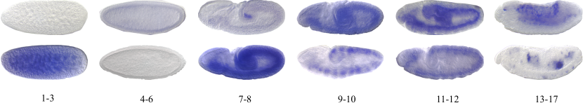
However, ISH images obtained from high-throughput experiments are commonly annotated with stage range labels, as illustrated by Figure 1. since determining the precise stage for each ISH image is very hard and time-consuming even for expert biologists. Currently, most of the comparative analysis is limited to stage range levels due to the lack of accurate and cost-effective methods for assigning precise stage labels to images. In [13], a small training set is manually labeled with precise stages by developmental biologists, and a computational pipeline is proposed to train classifiers from this small training set. Specifically, pre-defined Gabor filters are used to compute features from ISH images [7, 14] and linear classifiers are employed to predict the precise stages of ISH images. In that work, no attempt is made to explicitly consider and account for the key bottleneck of limited training samples. Due to the small size of training set and the methods used, the predictive performance is relatively poor in that work. In order for the results to be usable by routine biological studies, an accurate computational model that can be trained effectively from limited training samples is highly desirable [15, 16, 17, 18].
We notice that the Gabor filter features used in [13] are computed by convolving a set of pre-defined filters to input images. Although the pre-defined Gabor filters have been widely used, the filter weights are pre-computed and extract features that do not adapt to each task and data specifically. In order to enable automated data-driven and task-related feature extraction, we propose to employ deep convolutional neural networks (DCNNs) for this task [19]. However, DCNNs require a large number of training samples to estimate the filter weights while most biological applications, including the precise stage prediction task of ISH images that we are considering, have only very limited training samples. Thus, straightforward use of CNNs inevitably results in poor performance.
In this work, we propose a deep two-step low-shot learning framework that consists of a set of novel computational techniques to enable effective deep model training on a small number of annotated training samples. Although we focus on ISH image classification and visualization in this work, the proposed approach is generic and can be easily generalizable to other biological image analysis tasks. Specifically, we formulate the original classification task with limited training samples as a deep low-shot learning problem [20, 21, 22] and propose a deep two-step low-shot learning approach that consists of data-level learning and feature-level learning. The first data-level learning step leverages extra data to facilitate the training. In the precise stage prediction task of ISH images, we can access a large number of extra ISH images with stage range labels, which cannot be directly used to train a precise stage prediction model. However, these extra ISH images are obtained from the same experimental pipeline and follow the same distribution as images in the original small training set. Therefore, they can be exploited to guide the training. The second step of our low-shot learning method is feature-level learning. We propose a regularization method which forces a high similarity of features extracted from different samples in the same class. It results in a high-quality feature space, enabling the extracted features to generalize well on unseen data. In order to achieve the regularization for classification, we generate reference sets that contain representative samples of each class. The proposed feature-level learning step is to fine-tune the model by adding a similarity loss based on cosine similarities between features extracted from the training sample and reference samples. The proposed deep two-step low-shot learning framework enables us to effectively train deep learning models with high classification accuracy. In addition, we explore the interpretation of deep learning models through saliency maps [23], which indicate pixel-wise contributions of input images to the prediction results. In the precise stage prediction task of ISH images, we generate masked genomewide expression maps (GEMs) [24, 25] based on saliency maps. The masked GEMs provide biologically meaningful visualizations that help identifying and visualizing developmental landmarks.
II A Deep Two-Step Low-Shot Learning Framework
In this section, we introduce our deep two-step low-shot learning framework. We start with the motivation, advantages and challenges of applying deep learning on biological image classification in Section II-A. To overcome the challenges, we formulate the task as a deep low-shot learning problem and propose the deep two-step low-shot learning approach to address it. The two steps, namely data-level learning and feature-level learning, are described in Sections II-B and II-C, respectively. In Section II-D, we apply the proposed method with a deep residual network on the precise stage prediction task of ISH images. We also introduce the interpretation method for deep learning models and how to use it to generate biologically meaningful visualizations for our task in Section II-E.
II-A Deep Learning for Biological Image Classification
Many traditional biological image analyses involve a hand-crafted feature extraction step, which requires expertise and only focuses on specific types of features. An example is using the Gabor filter to obtain texture features for the stage prediction task of ISH images [13]. While hand-crafted features achieve acceptable performance in practice, they have two main disadvantages. First, it is expensive and time-consuming to design these feature extractors. There are a variety of biological images with different tasks, and each of which needs a re-design of feature extraction methods accordingly. Second, the performance is limited by human’s knowledge. However, more accurate analysis is needed to improve our understanding.
Deep learning has provided a promising way to perform automatic feature extraction in a data-driven and task-related manner [26]. Instead of relying on hand-crafted feature extractors, deep neural networks can learn to extract features through training on annotated data. Specifically, experts are only required to analyze and annotate a limited amount of data manually. Then, deep neural networks are able to determine features that are important to the task and design corresponding feature extractors. Based on them, the trained networks can perform the task on unlabeled data automatically, in an efficient and accurate way.
A key challenge of applying deep learning for biological image analysis is that the number of available annotated data is very limited, while deep learning models typically require a large amount of training data. It is usually cost-effective to perform coarse annotation on large-scale data. Fine annotation with high accuracy can only be done on a very small portion of data due to practical limitations of resources. It hinders the wide use of deep learning.
To address the challenge, we formulate it as a deep low-shot learning problem. In this problem, a large dataset with coarse labels and a small dataset with fine labels are available. To be specific, we denote the large dataset as and the small dataset as , where and , respectively. Here, and represent the number of annotated data in each dataset and we have . Correspondingly, and represent the number of classes in coarse and fine annotations, respectively. In this setting, it is reasonable to assume . Note that does not have the same meaning as , since coarse and fine annotations have different label space. The data samples in both datasets, and , are from the same distribution. The task is to develop accurate deep learning models to perform fine annotation. However, the small prevents us to directly train a deep neural network on , making it necessary to develop a method that is able to effectively leverage . To solve this problem, we propose a method combining data-level learning and feature-level learning, leading to our deep two-step low-shot learning approach.
II-B Data-Level Deep Low-Shot Learning
The first step of our proposed approach is data-level learning. Namely, we propose a way to leverage the large dataset and learn from more data, even when these data have coarse labels only. To introduce our method, we first review the deep classification networks.
A deep classification network is typically composed of a feature extraction network and a classification network. The feature extraction network corresponds to the hand-crafted feature extraction step in traditional methods and the classification network performs the task based on extracted features. We focus on the feature extraction network as extracting features of high quality is the key to achieving satisfactory classification performance. Based on good features, the task can be well solved by using simple machine learning methods like nearest neighbor algorithm and linear classification methods [27]. Actually, the classification networks in modern deep classification networks [19, 28] are usually equivalent to multi-class logistic regression. The classification network simply serves as a guide for feature extraction network to extract task-related features from given data.
Note that, in the deep low-shot learning problem defined in Section II-A, and are from the same distribution. In addition, and are labels of two different accuracy levels for the same classification task. With the insights above, we point out that training a deep classification network for the coarse annotation task on is able to provide an informative and useful feature extraction network for the ultimate fine annotation task.
Therefore, our data-level learning step proposes to first train a deep classification network on , where a large amount of annotated data are available. Specifically, the deep classification network consisting of a feature extraction network and a classification network is denoted as , where and represent the parameters in and , respectively. Note that performs classification based on coarse labels, whose output layer has nodes. After training on , we build another deep classification network to perform fine annotation. In particular, we employ the same extraction network and simply change the classification network to whose output layer has nodes. Finally, we train on . In terms of training, we let the outputs of the classification network to go through a Softmax function and compute the cross-entropy loss for back-propagation [26]. Taking as an example, for one training sample in , the Softmax function is defined as:
| (1) |
where denote the output of the -th node, i.e.,
| (2) |
Here, can be interpreted as the probability that the input image belongs to the -th class. The cross-entropy loss can be computed by:
| (3) |
which simply depends on the predicted probability that belongs to the -th class.
The key step of data-level learning is to apply the same feature extraction network in the process. Intuitively, such an approach enables the task-related knowledge obtained from to be transferred to . Technically, training on provides a good initialization for training on , alleviating the problem of lacking enough training data for the fine annotation task.
II-C Feature-Level Deep Low-Shot Learning
The second step of our proposed approach is feature-level learning, where we propose a regularization method to force a high similarity of features extracted from different samples in the same class. To achieve it, we select several samples from each class as reference samples and regularize the feature extraction network to extract similar features from other samples in the same class. We first describe how to select reference samples and then introduce the regularization method.
After the data-level learning step described in Section II-B, we obtain a deep classification network that has been trained on . Using the Softmax function in Equation (1), for each training sample in , we can compute the probability that belongs to . We set a threshold and select those samples with . The setting of should make sure that . Specifically, for each class , we obtain a subset of defined as . Note that these subsets , are mutually exclusive. Then, we randomly select one sample from each to form a reference set which contains exactly reference samples. The last step is iterated for times to form reference sets , .
The feature-level learning step follows the data-level learning by fine-tuning on with the help of reference sets , . When fine-tuning with one training sample in , we randomly pick a reference set from , . The feature-level learning aims to force the features extracted from input images in the same class to be similar, i.e., and should be similar. In opposite, for , and should be less similar. It requires a quantitative way to evaluate the similarity between features. In this work, we quantify the similarity by calculating:
| (4) | |||||
For each , we can compute the corresponding . Then, we normalize the similarities through a Softmax function:
| (5) |
where a large means that and are similar. At last, we propose the similarity loss:
| (6) | |||||
Minimizing the similarity loss will result in maximizing while minimizing for . This corresponds to our purpose of forcing features extracted from input images in the same class to be similar as well as making those in different classes distinguishable. Therefore, the similarity loss serves as a feature-level regularization method. When fine-tuning the deep classification network in the feature-level learning step, we apply a combined loss function defined as:
| (7) |
where is defined by Equation (3).
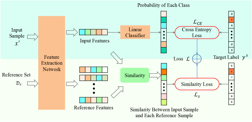
An overview of the proposed feature-level learning step is provided in Figure 2. The feature-level learning provides better features for the fine annotation task and improves .
II-D Deep Two-Step Low-Shot Learning for the Precise Stage Prediction of ISH Images
Combining data-level learning and feature-level learning leads to our proposed deep two-step low-shot learning approach, shown in Algorithm 1. We apply this approach to solve the precise stage prediction task of Drosophila ISH images [13]. In this task, the large dataset with coarse labels refers to the ISH images with stage range labels as illustrated in Figure 1. These labels only indicate that the developmental stage of an ISH image falls into one of the six ranges. Meanwhile, a small dataset with fine labels is available, where the data are annotated with precise stages. Here, and , respectively. The precise stage prediction task can be well formulated as a deep low-shot learning problem and addressed by our proposed method.
Deep convolutional neural networks (DCNNs) [26] have achieved great success in various image tasks. Convolutional layers are proved to be capable of performing effective feature extraction. Therefore, we use DCNNs as our deep learning model for the precise stage prediction task. In particular, we apply a deep residual network (ResNet) by adopting the technique of adding residual connections proposed in [19]. Residual connections are known to facilitate the training of deep neural networks.
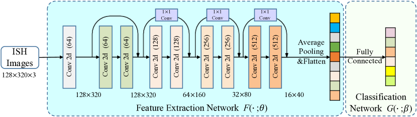
Figure 3 illustrates our deep residual network for the stage prediction task. Our feature extraction network contains four residual blocks, each of which is composed of two convolutional layers and a residual connection. A convolutional layer contains a convolution followed by a batch normalization [29] and a ReLU activation function [30]. A residual connection is employed to add the inputs to the outputs for two consecutive convolutional layers and forms a residual block. The residual connection is simply an identity connection for the first residual block. For the latter three residual blocks, we set the stride to 2 for the first convolutional layer, resulting in outputs of reduced spatial sizes. In this case, we use a convolutional layer in the residual connection, which changes the spatial sizes of inputs accordingly to accommodate the addition. We apply an average pooling with a kernel size of to obtain the extracted features after the last residual block. The classification networks and are designed as a single fully-connected layer with and output nodes, respectively. Our deep learning model is trained by following Algorithm 1 and outperforms the previous state-of-the-art model [13] significantly, as shown in Section IV.
II-E Interpretation and Visualization Using Saliency Maps
Our proposed deep two-step low-shot learning approach yields deep learning models with high accuracy. We further introduce an interpretation method for deep learning models based on saliency maps. Saliency maps quantify the pixel-wise contributions of an input image to its prediction result by computing the gradient of the prediction outputs with respect to the input image [23]. To be specific, to interpret our deep classification network with input image , we compute the saliency maps for each output node:
| (8) |
where is defined in Equation (2). Suppose the prediction result of is . We pay attention to as it tells which pixels in support the prediction result most.
In the precise stage prediction task of ISH images, we apply saliency maps to generate masked genomewide expression maps (GEMs) to help identifying and visualizing developmental landmarks. GEMs provide a visualization method for precise stage prediction models and a visualization method for developmental landmark analysis. Originally, GEMs are generated by aggregating and normalizing the ISH images from the same stage [24, 25]. We propose to use saliency maps as masks in generating GEMs, selecting characteristic pixels from ISH images that contribute to the prediction results. We show that the resulted masked GEMs can provide more biologically meaningful visualizations in Section IV.
| Stage |
|
|
Stage |
|
|
||||||||
| 1-3 | 0 | 4203 | 11 | 246 | 9248 | ||||||||
| 4 | 251 | 7344 | 12 | 255 | |||||||||
| 5 | 274 | 13 | 251 | 8680 | |||||||||
| 6 | 224 | 14 | 252 | ||||||||||
| 7 | 236 | 3665 | 15 | 232 | |||||||||
| 8 | 260 | 16 | 243 | ||||||||||
| 9 | 248 | 3768 | 17 | 254 | |||||||||
| 10 | 248 | Total | 3474 | 36908 |
| Model |
|
|
|
|
|
|
|
|
||||||||
|---|---|---|---|---|---|---|---|---|---|---|---|---|---|---|---|---|
| Gabor Filter [13] | 84% | 83% | 91% | 95% | 82% | 62% | 64% | 85% | ||||||||
| Plain ResNet | 81% | 77% | 81% | 90% | 80% | 57% | 53% | 83% | ||||||||
| Data-level | 76% | 91% | 85% | 99% | 84% | 66% | 66% | 86% | ||||||||
| Data&Feature-level | 81% | 89% | 87% | 98% | 87% | 75% | 64% | 84% | ||||||||
| Model |
|
|
|
|
|
|
Average | |||||||||
| Gabor Filter [13] | 80% | 94% | 74% | 86% | 73% | 80% | 80.97% | |||||||||
| Plain ResNet | 80% | 89% | 77% | 77% | 72% | 80% | 77.28% | |||||||||
| Data-level | 88% | 92% | 84% | 74% | 71% | 84% | 82.40% | |||||||||
| Data&Feature-level | 89% | 94% | 79% | 81% | 74% | 87% | 83.92% |
III Related Work
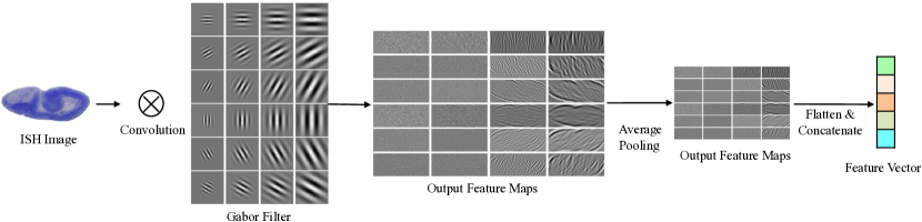
Currently, the state-of-the-art method [13] for the precise stage prediction task of ISH images is to extract features using pre-defined convolutional filters and train a linear classifier based on the extracted features. Texture features of different scales and orientations can be computed with different filters. The filter weights are constructed by using log Gabor filters [7, 14]. Given a set of pre-defined wavelet scales and orientations, we can generate corresponding Gabor filters to extract the specific features by convolving on input images. The precise stage prediction model in [13] based on Gabor filter features is illustrated in Figure 4.
The Gabor filter features focus on subtle textures which enable the classification model to distinguish ISH images from different stages. However, there are still some limitations for Gabor filter features as Gabor filters are hand-crafted and cannot learn features automatically for different tasks and datasets. Moreover, Gabor filters only extract low-level texture features. Extracting features hierarchically from low-level to high-level is appealing for improving the precise stage prediction accuracy.
IV Experimental Studies
In this section, we evaluate our proposed deep two-step low-shot learning framework for the precise stage prediction task of ISH images on the Berkeley Drosophila Genome Project (BDGP) dataset. We perform qualitative evaluation in terms of the prediction accuracy as well as qualitative evaluation based on feature visualization and genomewide expression maps (GEMs) [25, 24]. Finally, we show the saliency maps and masked GEMs for interpretation and visualization.

IV-A Experimental Setup
The BDGP dataset contains 36908 Drosophila ISH images in lateral view. Among them, only 3474 ISH images are annotated with precise stage labels. In addition, all images are labeled into six stage ranges: 1-3, 4-6, 7-8, 9-10, 11-12 and 13-17 as illustrated in Figure 1. According to Section II-D, we have with and with , respectively. The details are listed in Table I. Note that, since the Drosophila embryogenesis is not very meaningful from stage 1 to stage 3, the precise stage prediction task does not involving this range. Therefore, there is no precise stage annotation for this range. All ISH images are standardized by the pipeline proposed in [24], and the size of processed images is . To perform evaluation, we randomly select of images for training and test our proposed model on the rest images.
We use the previous state-of-the-art model proposed in [13] that use Gabor filters as our baseline. For deep learning, we use the ResNet introduced in Section II-D. To show the effectiveness of our proposed deep two-step low-shot learning approach, we compare the performance of our ResNet trained using three different approaches: train it directly on (Plain ResNet), train it using data-level low-shot learning only (Data-level), and train it using both data-level and feature-level low-shot learning (Data&Feature-level). For all training processes, we employ the stochastic gradient descent algorithm [26]. The learning rate starts with 0.001 and is multiplied by 0.1 at the 20-th and 30-th epoch. The batch size is set to 16.
IV-B Quantitative Analysis of Predictive Performance
The precise stage prediction accuracy of each method is reported in Table II. Note that the accuracy of Plain ResNet is lower than that of our baseline model, proving that deep learning models can hardly achieve satisfactory performance with limited training samples. Training the ResNet with our data-level deep low-shot learning method addresses this problem effectively and improves the performance significantly. By adding the feature-level learning step, our proposed deep two-step low-shot learning model achieves better predictive performance and becomes the new state-of-the-art model for the precise stage prediction task of ISH images.
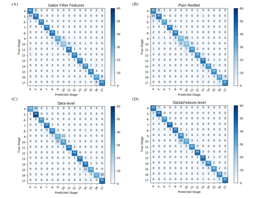
In order to analyze the prediction errors of our model, we compare the confusion matrices of the prediction results, as shown in Figure 5. We observe that most wrongly-predicted samples are classified into neighboring stages, within the correct stage ranges. In particular, for deep learning models trained using our proposed low-shot learning methods, the number of samples that are categorized into wrong stage ranges is fewer than the baseline. It indicates that the data-level deep low-shot learning step effectively incorporates information from samples with stage range labels and improves the performance of precise stage prediction.
IV-C Qualitative Analysis of Predictive Performance
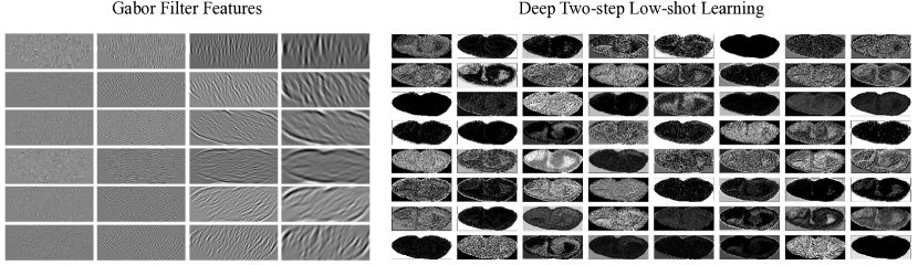
We perform two qualitative analyses on the baseline and the proposed deep two-step low-shot learning model. First, we compare the features extracted by Gabor filters with those generated by the first convolutional layer in the proposed model. Figure 6 provides visualizations of the features. Clearly, Gabor filters can only extract pre-defined low-level texture features while our deep learning model is able to extract data-driven and task-related features automatically. Our deep two-step low-shot learning framework takes advantage of the power of deep learning models by proposing effective training approaches and yields improved performance.
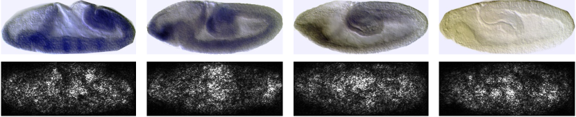
Second, we visualize genomewide expression maps (GEMs) [24, 25] generated by the baseline and our deep two-step low-shot learning model. Computing GEMs relies on the predictive performance and accurate precise stage prediction results produce more biologically meaningful GEMs. The first two columns in Figure 7 compare the GEMs generated using prediction results of the baseline and our model. According to the third column, we can see that the developing trend shown in both GEMs is consistent with that shown in [31]. In addition, since our proposed method achieves better predictive performance, the generated GEMs contain more biologically meaningful details as demonstrated by yellow bounding boxes. The differences can be better observed when zooming in the Figure 7.
IV-D Visualization through Salience Maps and Masked Genomewide Expression Maps
As introduced in Section II-E, we can compute saliency maps to measure the pixel-wise contributions of an input image to its prediction result. We visualize some saliency maps generated by our proposed two-step low-shot learning model in Figure 8. From the saliency maps, we can infer which pixels contribute most to the prediction results. We propose to apply saliency maps as masks and use these pixels to generate GEMs instead of using the whole input images. The resulted masked GEMs are shown in the last column in Figure 7. The masked GEMs also show a consistent developing trend as shown in the third column. Moreover, they provide better visualizations to help identifying and visualizing developmental landmarks.
V Conclusion
In this work, we propose a deep two-step low-shot learning framework and apply it on the precise stage prediction task of ISH images. We first propose to employ deep learning models to automatically extract data-driven and task-related features instead of using hand-crafted feature extraction methods. In order to build accurate deep learning models from limited training samples, we formulate the task as a deep low-shot learning problem. To solve it, we propose a deep two-step low-shot learning approach that is composed of data-level learning and feature-level learning. The first data-level learning step leverages extra data to facilitate the training. The second step, feature-level learning, introduces a regularization method which forces a high similarity of features extracted from different samples in the same class. The proposed deep two-step low-shot learning framework enables us to effectively train deep learning models with high classification accuracy. We conduct thorough experiments on the BDGP dataset using a deep residual network as our base model. Both quantitative and qualitative experimental results demonstrate that our proposed deep two-step low-shot model outperforms the previous state-of-the-art model significantly. In addition, we explore visualization based on saliency maps [23], which compute pixel-wise contributions of input images to the prediction results. In the precise stage prediction task of ISH images, we apply saliency maps to generate masked genomewide expression maps, which provide biologically meaningful visualizations that help identifying and visualizing developmental landmarks [32].
Acknowledgment
This work was supported in part by National Science Foundation Grants IIS-1908220 and DBI-1661289.
References
- [1] T. Zeng, R. Li, R. Mukkamala, J. Ye, and S. Ji, “Deep convolutional neural networks for annotating gene expression patterns in the mouse brain,” BMC Bioinformatics, vol. 16, p. 147, 2015.
- [2] A. Cardona and P. Tomancak, “Current challenges in open-source bioimage informatics,” nature methods, vol. 9, no. 7, p. 661, 2012.
- [3] T. Walter, D. W. Shattuck, R. Baldock, M. E. Bastin, A. E. Carpenter, S. Duce, J. Ellenberg, A. Fraser, N. Hamilton, S. Pieper et al., “Visualization of image data from cells to organisms,” Nature methods, vol. 7, no. 3s, p. S26, 2010.
- [4] H. Peng, F. Long, J. Zhou, G. Leung, M. B. Eisen, and E. W. Myers, “Automatic image analysis for gene expression patterns of fly embryos,” BMC cell biology, vol. 8, no. 1, p. S7, 2007.
- [5] E. Lécuyer, H. Yoshida, N. Parthasarathy, C. Alm, T. Babak, T. Cerovina, T. R. Hughes, P. Tomancak, and H. M. Krause, “Global analysis of mrna localization reveals a prominent role in organizing cellular architecture and function,” Cell, vol. 131, no. 1, pp. 174–187, 2007.
- [6] P. Tomancak, A. Beaton, R. Weiszmann, E. Kwan, S. Shu, S. E. Lewis, S. Richards, M. Ashburner, V. Hartenstein, S. E. Celniker et al., “Systematic determination of patterns of gene expression during drosophila embryogenesis,” Genome biology, vol. 3, no. 12, pp. research0088–1, 2002.
- [7] J. G. Daugman, “Two-dimensional spectral analysis of cortical receptive field profiles,” Vision research, vol. 20, no. 10, pp. 847–856, 1980.
- [8] M. Levine and E. H. Davidson, “Gene regulatory networks for development,” Proceedings of the National Academy of Sciences, vol. 102, no. 14, pp. 4936–4942, 2005.
- [9] S. Kumar, K. Jayaraman, S. Panchanathan, R. Gurunathan, A. Marti-Subirana, and S. J. Newfeld, “BEST: a novel computational approach for comparing gene expression patterns from early stages of Drosophila melanogaster develeopment,” Genetics, vol. 169, pp. 2037–2047, 2002.
- [10] E. Frise, A. S. Hammonds, and S. E. Celniker, “Systematic image-driven analysis of the spatial Drosophila embryonic expression landscape,” Molecular Systems Biology, vol. 6, p. 345, 2010.
- [11] H. Peng and E. W. Myers, “Comparing in situ mRNA expression patterns of Drosophila embryos,” in Proceedings of the Eighth Annual International Conference on Resaerch in Computational Molecular Biology. New York, NY, USA: ACM, 2004, pp. 157–166.
- [12] P. Tomancak, B. P. Berman, A. Beaton, R. Weiszmann, E. Kwan, V. Hartenstein, S. E. Celniker, and G. M. Rubin, “Global analysis of patterns of gene expression during drosophila embryogenesis,” Genome biology, vol. 8, no. 7, p. R145, 2007.
- [13] L. Yuan, C. Pan, S. Ji, M. McCutchan, Z.-H. Zhou, S. J. Newfeld, S. Kumar, and J. Ye, “Automated annotation of developmental stages of drosophila embryos in images containing spatial patterns of expression,” Bioinformatics, vol. 30, no. 2, pp. 266–273, 2013.
- [14] D. J. Field, “Relations between the statistics of natural images and the response properties of cortical cells,” Josa a, vol. 4, no. 12, pp. 2379–2394, 1987.
- [15] S. Ji, L. Sun, R. Jin, S. Kumar, and J. Ye, “Automated annotation of drosophila gene expression patterns using a controlled vocabulary,” Bioinformatics, vol. 24, no. 17, pp. 1881–1888, 2008.
- [16] J. Ye, J. Chen, Q. Li, and S. Kumar, “Classification of drosophila embryonic developmental stage range based on gene expression pattern images,” in Computational Systems Bioinformatics. World Scientific, 2006, pp. 293–298.
- [17] X. Cai, H. Wang, H. Huang, and C. Ding, “Joint stage recognition and anatomical annotation of Drosophila gene expression patterns,” Bioinformatics, vol. 28, no. 12, pp. i16–i24, 2012.
- [18] V. Hartenstein, Atlas of Drosophila Development. Cold Spring Harbor, NY: Cold Spring Harbor Laboratory Press, 1995.
- [19] K. He, X. Zhang, S. Ren, and J. Sun, “Deep residual learning for image recognition,” in Proceedings of the IEEE conference on computer vision and pattern recognition, 2016, pp. 770–778.
- [20] L. Fei-Fei, R. Fergus, and P. Perona, “One-shot learning of object categories,” IEEE transactions on pattern analysis and machine intelligence, vol. 28, no. 4, pp. 594–611, 2006.
- [21] B. Lake, R. Salakhutdinov, J. Gross, and J. Tenenbaum, “One shot learning of simple visual concepts,” in Proceedings of the Annual Meeting of the Cognitive Science Society, vol. 33, no. 33, 2011.
- [22] Y.-X. Wang, R. Girshick, M. Hebert, and B. Hariharan, “Low-shot learning from imaginary data,” arXiv preprint arXiv:1801.05401, 2018.
- [23] K. Simonyan, A. Vedaldi, and A. Zisserman, “Deep inside convolutional networks: Visualising image classification models and saliency maps,” arXiv preprint arXiv:1312.6034, 2013.
- [24] C. E. Konikoff, T. L. Karr, M. McCutchan, S. J. Newfeld, and S. Kumar, “Comparison of embryonic expression within multigene families using the flyexpress discovery platform reveals more spatial than temporal divergence,” Developmental Dynamics, vol. 241, no. 1, pp. 150–160, 2012.
- [25] S. Kumar, C. Konikoff, B. Van Emden, C. Busick, K. T. Davis, S. Ji, L.-W. Wu, H. Ramos, T. Brody, S. Panchanathan et al., “Flyexpress: visual mining of spatiotemporal patterns for genes and publications in drosophila embryogenesis,” Bioinformatics, vol. 27, no. 23, pp. 3319–3320, 2011.
- [26] Y. LeCun, L. Bottou, Y. Bengio, and P. Haffner, “Gradient-based learning applied to document recognition,” Proceedings of the IEEE, vol. 86, no. 11, pp. 2278–2324, 1998.
- [27] J. Snell, K. Swersky, and R. Zemel, “Prototypical networks for few-shot learning,” in Advances in Neural Information Processing Systems, 2017, pp. 4077–4087.
- [28] K. He, X. Zhang, S. Ren, and J. Sun, “Identity mappings in deep residual networks,” in European conference on computer vision. Springer, 2016, pp. 630–645.
- [29] S. Ioffe and C. Szegedy, “Batch normalization: Accelerating deep network training by reducing internal covariate shift,” in International Conference on Machine Learning, 2015, pp. 448–456.
- [30] A. Krizhevsky, I. Sutskever, and G. E. Hinton, “Imagenet classification with deep convolutional neural networks,” in Advances in neural information processing systems, 2012, pp. 1097–1105.
- [31] V. Hartenstein, “Atlas of drosophila development. 1993,” Plainview, NY: Cold Spring Harbor Laboratory Press. v.
- [32] H. Wang, C. Deng, H. Zhang, X. Gao, and H. Huang, “Drosophila gene expression pattern annotations via multi-instance biological relevance learning,” in Thirtieth AAAI Conference on Artificial Intelligence, 2016.