Improving Factual Completeness and Consistency of
Image-to-Text Radiology Report Generation

Abstract

Neural image-to-text radiology report generation systems offer the potential to improve radiology reporting by reducing the repetitive process of report drafting and identifying possible medical errors. However, existing report generation systems, despite achieving high performances on natural language generation metrics such as CIDEr or BLEU, still suffer from incomplete and inconsistent generations. Here we introduce two new simple rewards to encourage the generation of factually complete and consistent radiology reports: one that encourages the system to generate radiology domain entities consistent with the reference, and one that uses natural language inference to encourage these entities to be described in inferentially consistent ways. We combine these with the novel use of an existing semantic equivalence metric (BERTScore). We further propose a report generation system that optimizes these rewards via reinforcement learning. On two open radiology report datasets, our system substantially improved the ${\rm F}_{1}$ score of a clinical information extraction performance by $+22.1$ ($\Delta+63.9\%$). We further show via a human evaluation and a qualitative analysis that our system leads to generations that are more factually complete and consistent compared to the baselines.

1 Introduction

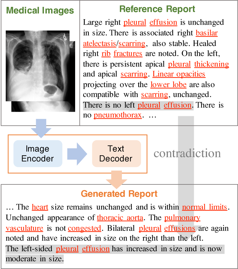
Figure 1: A (partial) example of a report generated from our system (with “…” representing abbreviated text). The system encodes images and generates text from that encoded representation. Underlined words are disease and anatomy entities. The shaded sentences are an example of a contradictory pair.

An important new application of natural language generation (NLG) is to build assistive systems that take X-ray images of a patient and generate a textual report describing clinical observations in the images Jing et al. (2018); Li et al. (2018); Liu et al. (2019); Boag et al. (2020); Chen et al. (2020). Figure 1 shows an example of a radiology report generated by such a system. This is a clinically important task, offering the potential to reduce radiologists’ repetitive work and generally improve clinical communication Kahn et al. (2009).

Automatic radiology report generation systems have achieved promising performance as measured by widely used NLG metrics such as CIDEr Vedantam et al. (2015) and BLEU Papineni et al. (2002) on several datasets Li et al. (2018); Jing et al. (2019); Chen et al. (2020). However, reports that achieve high performance on these NLG metrics are not always factually complete or consistent. In addition to the use of inadequate metrics, the factual incompleteness and inconsistency issue in generated reports is further exacerbated by the inadequate training of these systems. Specifically, the standard teacher-forcing training algorithm Williams and Zipser (1989) used by most existing work can lead to a discrepancy between what the model sees during training and test time Ranzato et al. (2016), resulting in degenerate outputs with factual hallucinations Maynez et al. (2020). Liu et al. (2019) and Boag et al. (2020) have shown that reports generated by state-of-the-art systems still have poor quality when evaluated by their clinical metrics as measured with an information extraction system designed for radiology reports. For example, the generated report in Figure 1 is incomplete since it neglects an observation of atelectasis that can be found in the images. It is also inconsistent since it mentions left-sided pleural effusion which is not present in the images. Indeed, we show that existing systems are inadequate in factual completeness and consistency, and that an image-to-text radiology report generation system can be substantially improved by replacing widely used NLG metrics with simple alternatives.

We propose two new simple rewards that can encourage the factual completeness and consistency of the generated reports. First, we propose the Exact Entity Match Reward ($\mathrm{fact}_{\mathrm{ENT}}$) which captures the completeness of a generated report by measuring its coverage of entities in the radiology domain, compared with a reference report. The goal of the reward is to better capture disease and anatomical knowledge that are encoded in the entities. Second, we propose the Entailing Entity Match Reward ($\mathrm{fact}_{\mathrm{ENTNLI}}$), which extends ${\rm fact_{ENT}}$ with a natural language inference (NLI) model that further considers how inferentially consistent the generated entities are with their descriptions in the reference. We add NLI to control the overestimation of disease when optimizing towards $\mathrm{fact}_{\mathrm{ENT}}$. We use these two metrics along with an existing semantic equivalence metric, BERTScore Zhang et al. (2020a), to potentially capture synonyms (e.g., “left and right” effusions are synonymous with “bilateral” effusions) and distant dependencies between diseases (e.g., a negation like “…but underlying consolidation or other pulmonary lesion not excluded”) that are present in radiology reports.

Although recent work in summarization, dialogue, and data-to-text generation has tried to address this problem of factual incompleteness and inconsistency by using natural language inference (NLI) Falke et al. (2019); Welleck et al. (2019), question answering (QA) Wang et al. (2020a), or content matching constraint Wang et al. (2020b) approaches, they either show negative results or are not directly applicable to the generation of radiology reports due to a substantial task and domain difference. To construct the NLI model for $\mathrm{fact}_{\mathrm{ENTNLI}}$, we present a weakly supervised approach that adapts an existing NLI model to the radiology domain. We further present a report generation model which directly optimizes a Transformer-based architecture with these rewards using reinforcement learning (RL).

We evaluate our proposed report generation model on two publicly available radiology report generation datasets. We find that optimizing the proposed rewards along with BERTScore by RL leads to generated reports that achieve substantially improved performance in the important clinical metrics Liu et al. (2019); Boag et al. (2020); Chen et al. (2020), demonstrating the higher clinical value of our approach. We make all our code and the expert-labeled test set for evaluating the radiology NLI model publicly available to encourage future research. To summarize, our contributions in this paper are:

1. We propose two simple rewards for image-to-text radiology report generation, which focus on capturing the factual completeness and consistency of generated reports, and a weak supervision-based approach for training a radiology-domain NLI model to realize the second reward.

2. We present a new radiology report generation model that directly optimizes these new rewards with RL, showing that previous approaches that optimize traditional NLG metrics are inadequate, and that the proposed approach substantially improves performance on clinical metrics (as much as $\Delta+64.2\%$) on two publicly available datasets.

2 Related Work

2.1 Image-to-Text Radiology Report Generation

Wang et al. (2018) and Jing et al. (2018) first proposed multi-task learning models that jointly generate a report and classify disease labels from a chest X-ray image. Their models were extended to use multiple images Yuan et al. (2019), to adopt a hybrid retrieval-generation model Li et al. (2018), or to consider structure information Jing et al. (2019). More recent work has focused on generating reports that are clinically consistent and accurate. Liu et al. (2019) presented a system that generates accurate reports by fine-tuning it with their Clinically Coherent Reward. Boag et al. (2020) evaluated several baseline generation systems with clinical metrics and found that standard NLG metrics are ill-equipped for this task. Very recently, Chen et al. (2020) proposed an approach to generate radiology reports with a memory-driven Transformer. Our work is most related to Liu et al. (2019); their system, however, is dependent on a rule-based information extraction system specifically created for chest X-ray reports and has limited robustness and generalizability to different domains within radiology. By contrast, we aim to develop methods that improve the factual completeness and consistency of generated reports by harnessing more robust statistical models and are easily generalizable.

2.2 Consistency and Faithfulness in Natural Language Generation

A variety of recent work has focused on consistency and faithfulness in generation. Our work is inspired by Falke et al. (2019), Welleck et al. (2019), and Matsumaru et al. (2020) in using NLI to rerank or filter generations in text summarization, dialogue, and headline generations systems, respectively. Other attempts in this direction include evaluating consistency in generations using QA models Durmus et al. (2020); Wang et al. (2020a); Maynez et al. (2020), with distantly supervised classifiers Kryściński et al. (2020), and with task-specific content matching constraints Wang et al. (2020b). Liu et al. (2019) and Zhang et al. (2020b) studied improving the factual correctness in generating radiology reports with rule-based information extraction systems. Our work mainly differs from theirs in the direct optimization of factual completeness with an entity-based reward and of factual consistency with a statistical NLI-based reward.

2.3 Image Captioning with Transformer

The problem of generating text from image data has been widely studied in the image captioning setting. While early work focused on combining convolutional neural network (CNN) and recurrent neural network (RNN) architectures Vinyals et al. (2015), more recent work has discovered the effectiveness of using the Transformer architecture Vaswani et al. (2017). Li et al. (2019) and Pan et al. (2020) introduced an attention process to exploit semantic and visual information into this architecture. Herdade et al. (2019), Cornia et al. (2020), and Guo et al. (2020) extended this architecture to learn geometrical and other relationships between input regions. We find Meshed-Memory Transformer Cornia et al. (2020) ($\mathcal{M}^{2}$ Trans) to be more effective in our radiology report generation task than the traditional RNN-based models and Transformer models (an empirical result will be shown in §4), and therefore use it as our base architecture.

3 Methods

3.1 Image-to-Text Radiology Report Generation with $\boldsymbol{\mathcal{M}^{2}}$ Trans

Formally, given $K$ individual images $x_{1\ldots K}$ of a patient, our task involves generating a sequence of words to form a textual report $\hat{y}$, which describes the clinical observations in the images. This task resembles image captioning, except with multiple images as input and longer text sequences as output. We therefore extend a state-of-the-art image captioning model, $\mathcal{M}^{2}$ Trans Cornia et al. (2020), with multi-image input as our base architecture. We first briefly introduce this model and refer interested readers to Cornia et al. (2020).

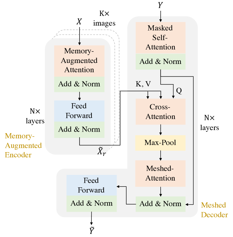
Figure 2: An overview of Meshed-Memory Transformer extended to multiple images.

Figure 2 illustrates an overview of the $\mathcal{M}^{2}$ Trans model. Given an image $x_{k}$, image regions are first extracted with a CNN as $\boldsymbol{X}=\mathrm{CNN}(x_{k})$. $\boldsymbol{X}$ is then encoded with a memory-augmented attention process $\mathcal{M}_{\mathrm{mem}}(\boldsymbol{X})$ as

$$\mathcal{M}_{\rm{mem}}(\boldsymbol{X}) =\rm{Att}(W_{q}\boldsymbol{X},\boldsymbol{K},\boldsymbol{V})$$ (1)

$$\rm{Att}(\boldsymbol{Q},\boldsymbol{K},\boldsymbol{V}) =\mathrm{softmax}\left(\frac{\boldsymbol{Q}\boldsymbol{K}^{T}}{\sqrt{d}}\right)\boldsymbol{V}$$ (2)

$$\boldsymbol{K} =[W_{k}\boldsymbol{X};\boldsymbol{M}_{k}]$$ (3)

$$\boldsymbol{V} =[W_{v}\boldsymbol{X};\boldsymbol{M}_{v}]$$ (4)

where $W_{q},W_{k},W_{v}$ are weights, $\boldsymbol{M}_{k},\boldsymbol{M}_{v}$ are memory matrices, $d$ is a scaling factor, and $[*;*]$ is the concatenation operation. $\rm{Att}(\boldsymbol{Q},\boldsymbol{K},\boldsymbol{V})$ is an attention process derived from the Transformer architecture Vaswani et al. (2017) and extended to include memory matrices that can encode a priori knowledge between image regions. In the encoder, this attention process is a self-attention process since all of the query $\boldsymbol{Q}$, the key $\boldsymbol{K}$, and the value $\boldsymbol{V}$ depend on $\boldsymbol{X}$. $\mathcal{M}_{\mathrm{mem}}(\boldsymbol{X})$ is further processed with a feed forward layer, a residual connection, and a layer normalization to output $\tilde{\boldsymbol{X}}$. This encoding process can be stacked $N$ times and is applied to $K$ images, and $n$-th layer output of $K$ image will be $\tilde{\boldsymbol{X}}_{n,\boldsymbol{K}}$.

The meshed decoder first processes an encoded text $\boldsymbol{Y}$ with a masked self-attention and further processes it with a feed forward layer, a residual connection, and a layer normalization to output $\ddot{\boldsymbol{Y}}$. $\ddot{\boldsymbol{Y}}$ is then passed to a cross attention $\mathcal{C}(\tilde{\boldsymbol{X}}_{n,\boldsymbol{K}},\ddot{\boldsymbol{Y}})$ and a meshed attention $\mathcal{M}_{\mathrm{mesh}}(\tilde{\boldsymbol{X}}_{\boldsymbol{N},\boldsymbol{K}},\ddot{\boldsymbol{Y}})$ as

$$\mathcal{M}_{\mathrm{mesh}}(\tilde{\boldsymbol{X}}_{\boldsymbol{N},\boldsymbol{K}},\ddot{\boldsymbol{Y}})=\sum_{n}\boldsymbol{\alpha}_{n}\odot\mathcal{C}(\tilde{\boldsymbol{X}}_{n,\boldsymbol{K}},\ddot{\boldsymbol{Y}})$$ (5)

$$\mathcal{C}(\tilde{\boldsymbol{X}}_{n,\boldsymbol{K}},\ddot{\boldsymbol{Y}})=\max_{\boldsymbol{K}}(\rm{Att}(W_{q}\ddot{\boldsymbol{Y}},W_{k}\tilde{\boldsymbol{X}}_{n,\boldsymbol{K}},W_{v}\tilde{\boldsymbol{X}}_{n,\boldsymbol{K}}))$$ (6)

$$\boldsymbol{\alpha}_{n}=\sigma\left(W_{n}[\boldsymbol{Y};\mathcal{C}(\tilde{\boldsymbol{X}}_{n,\boldsymbol{K}},\ddot{\boldsymbol{Y}})]+b_{n}\right)$$ (7)

where $\odot$ is element-wise multiplication, $\max_{\boldsymbol{K}}$ is max-pooling over $K$ images, $\sigma$ is sigmoid function, $W_{n}$ is a weight, and $b_{n}$ is a bias. The weighted summation in $\mathcal{M}_{\rm mesh}(\tilde{\boldsymbol{X}}_{\boldsymbol{N},\boldsymbol{K}},\ddot{\boldsymbol{Y}})$ exploits both low-level and high-level information from the $N$ stacked encoder. Differing from the self-attention process in the encoder, the cross attention uses a query that depends on $\boldsymbol{Y}$ and a key and a value that depend on $\boldsymbol{X}$. $\mathcal{M}_{\mathrm{mesh}}(\tilde{\boldsymbol{X}}_{\boldsymbol{N},\boldsymbol{K}},\ddot{\boldsymbol{Y}})$ is further processed with a feed forward layer, a residual connection, and a layer normalization to output $\tilde{\boldsymbol{Y}}$. As like in the encoder, the decoder can be stacked $N$ times to output $\tilde{\boldsymbol{Y}}_{N}$. $\tilde{\boldsymbol{Y}}_{N}$ is further passed to a feed forward layer to output report $\hat{y}$.

3.2 Optimization with Factual Completeness and Consistency

3.2.1 Exact Entity Match Reward ($\boldsymbol{\mathrm{fact}_{\mathrm{ENT}}}$)

We designed an F-score entity match reward to capture factual completeness. This reward assumes that entities encode disease and anatomical knowledge that relates to factual completeness. A named entity recognizer is applied to $\hat{y}$ and the corresponding reference report $y$. Given entities $E_{\mathrm{gen}}$ and $E_{\mathrm{ref}}$ recognized from $y_{\mathrm{gen}}$ and $y_{\mathrm{ref}}$ respectively, precision (pr) and recall (rc) of entity match are calculated as

$$\mathrm{pr}_{\mathrm{ENT}} =\frac{\sum_{e\in E_{\mathrm{gen}}}\delta(e,E_{\mathrm{ref}})}{|E_{\mathrm{gen}}|}$$ (8)

$$\mathrm{rc}_{\mathrm{ENT}} =\frac{\sum_{e\in E_{\mathrm{ref}}}\delta(e,E_{\mathrm{gen}})}{|E_{\mathrm{ref}}|}$$ (9)

$$\delta(e,E) =\begin{cases}1,&\text{for }e\in E\\ 0,&\text{otherwise}\end{cases}$$ (10)

The harmonic mean of precision and recall is taken as $\mathrm{fact}_{\mathrm{ENT}}$ to reward a balanced match of entities. We used Stanza Qi et al. (2020) and its clinical models Zhang et al. (2020c) as a named entity recognizer for radiology reports. For example in the case of Figure 1, the common entities among the reference report and the generated report are pleural and effusion, resulting to $\mathrm{fact}_{\mathrm{ENT}}=33.3$.

3.2.2 Entailing Entity Match Reward ($\boldsymbol{\mathrm{fact}_{\mathrm{ENTNLI}}}$)

We additionally designed an F-score style reward that expands $\mathrm{fact}_{\mathrm{ENT}}$ with NLI to capture factual consistency. NLI is used to control the overestimation of disease when optimizing towards $\mathrm{fact}_{\mathrm{ENT}}$. In $\mathrm{fact}_{\mathrm{ENTNLI}}$, $\delta$ in Eq. 10 is expanded to

$$\scriptstyle\phi(e,E)=\begin{cases}1,&\text{for }e\in E\wedge\mathrm{NLI_{e}}(\boldsymbol{P},h)\neq\mathrm{contradiction}\\ 1,&\text{for }\mathrm{NLI_{e}}(\boldsymbol{P},h)=\mathrm{entailment}\\ 0,&\text{otherwise}\end{cases}$$ (11)

$${\rm NLI_{e}}(\boldsymbol{P},h)=nli(\hat{p},h)\text{ where }\hat{p}=\operatorname*{arg\,max}_{p\in\boldsymbol{P}}sim(h,p)$$ (12)

where $h$ is a sentence that includes $e$, $\boldsymbol{P}$ is all sentences in a counter part text (if $h$ is a sentence in a generated report, $\boldsymbol{P}$ is all sentences in the corresponding reference report), $nli(*,*)$ is an NLI function that returns an NLI label which is one of $\{\mathrm{entailment,neutral,contradiction}\}$, and $sim(*,*)$ is a text similarity function. We used BERTScore Zhang et al. (2020a) as $sim(*,*)$ in the experiments (the detail of BERTScore can be found in Appendix A). The harmonic mean of precision and recall is taken as $\mathrm{fact}_{\mathrm{ENTNLI}}$ to encourage a balanced factual consistency between a generated text and the corresponding reference text. For example in the case of Figure 1, the sentence “The left-sided pleural effusion has increased in size and is now moderate in size.” will be contradictory to “There is no left pleural effusion.” resulting in pleural and effusion being rejected in $y_{\mathrm{gen}}$.

3.2.3 Joint Loss for Optimizing Factual Completeness and Consistency

We integrate the proposed factual rewards into self-critical sequence training Rennie et al. (2017). An RL loss $\mathcal{L_{\mathrm{RL}}}$ is minimized as the negative expectation of the reward $r$. The gradient of the loss is estimated with a single Monte Carlo sample as

$$\nabla_{\theta}\mathcal{L}_{\mathrm{RL}}(\theta)=-\nabla_{\theta}\log P_{\theta}(\hat{y}_{sp}|x_{1\ldots K})\left(r(\hat{y}_{sp})-r(\hat{y}_{gd})\right)$$ (13)

where $\hat{y}_{sp}$ is a sampled text and $\hat{y}_{gd}$ is a greedy decoded text. Paulus et al. Paulus et al. (2018) and Zhang et al. Zhang et al. (2020b) have shown that a generation can be improved by combining multiple losses. We combine a factual metric loss with a language model loss and an NLG loss as

$$\mathcal{L} =\lambda_{1}\mathcal{L}_{\mathrm{NLL}}+\lambda_{2}\mathcal{L}_{\mathrm{RL\_NLG}}+\lambda_{3}\mathcal{L}_{\mathrm{RL\_FACT}}$$ (14)

where $\mathcal{L}_{\mathrm{NLL}}$ is a language model loss, $\mathcal{L}_{\mathrm{RL\_NLG}}$ is the RL loss using an NLG metric (e.g., CIDEr or BERTScore), $\mathcal{L}_{\mathrm{RL\_FACT}}$ is the RL loss using a factual reward (e.g., $\mathrm{fact}_{\mathrm{ENT}}$ or $\mathrm{fact}_{\mathrm{ENTNLI}}$), and $\lambda_{*}$ are scaling factors to balance the multiple losses.

3.3 A Weakly-Supervised Approach for Radiology NLI

We propose a weakly-supervised approach to construct an NLI model for radiology reports. (There already exists an NLI system for the medical domain, MedNLI Romanov and Shivade (2018), but we found that a model trained on MedNLI does not work well on radiology reports.) Given a large scale dataset of radiology reports, a sentence pair is sampled and filtered with weakly-supervised rules. The rules are prepared to extract a randomly sampled sentence pair ($s_{1}$ and $s_{2}$) that are in an entailment, neutral, or contradiction relation. We designed the following $6$ rules for weak-supervision.

Entailment 1 (E1)

(1) $s_{1}$ and $s_{2}$ are semantically similar and (2) NE of $s_{2}$ is a subset or equal to NE of $s_{1}$.

Neutral 1 (N1)

(1) $s_{1}$ and $s_{2}$ are semantically similar and (2) NE of $s_{1}$ is a subset of NE of $s_{2}$.

Neutral 2 (N2)

(1) NE of $s_{1}$ are equal to NE of $s_{2}$ and (2) $s_{1}$ include an antonym of a word in $s_{2}$.

Neutral 3 (N3)

(1) NE types of $s_{1}$ are equal to NE types of $s_{2}$ and (2) NE of $s_{1}$ is different from NE of $s_{2}$. NE types are used in this rule to introduce a certain level of similarity between $s_{1}$ and $s_{2}$.

Neutral 4 (N4)

(1) NE of $s_{1}$ are equal to NE of $s_{2}$ and (2) $s_{1}$ and $s_{2}$ include observation keywords.

Contradiction 1 (C1)

(1) NE of $s_{1}$ is equal or a subset to NE of $s_{2}$ and (2) $s_{1}$ is a negation of $s_{2}$.

The rules rely on a semantic similarity measure and the overlap of entities to determine the relationship between $s_{1}$ and $s_{2}$. In the neutral rules and the contradiction rule, we included similarity measures to avoid extracting easy to distinguish sentence pairs.

We evaluated this NLI by preparing training data, validation data, and test data. For the training data, the training set of MIMIC-CXR Johnson et al. (2019) is used as the source of sentence pairs. $2$k pairs are extracted for E1 and C1, $0.5$k pairs are extracted for N1, N2, N3, and N4, resulting in a total of $6$k pairs. The training set of MedNLI is also used as additional data. For the validation data and the test data, we sampled $480$ sentence pairs from the validation section of MIMIC-CXR and had them annotated by two experts: one medical expert and one NLP expert. Each pair is annotated twice swapping its premise and hypothesis resulting in $960$ pairs and are split in half resulting in $480$ pair for a validation set and $480$ pairs for a test set. The test set of MedNLI is also used as alternative test data.

Training Data	#samples	Test Accuracy
		RadNLI	MedNLI
MedNLI	$13$k	$53.3$	$\boldsymbol{80.9}$
MedNLI + RadNLI	$19$k	$\boldsymbol{77.8}$	$79.8$

Table 1: The accuracies of the NLI model trained with the weakly-supervised approach. RadNLI is the proposed NLI for radiology reports. The values are the average of $5$ runs and the bold values are the best results of each test set.

We used BERT Devlin et al. (2019) as an NLI model since it performed as a strong baseline in the existing MedNLI system Ben Abacha et al. (2019), and used Stanza Qi et al. (2020) and its clinical models Zhang et al. (2020c) as a named entity recognizer. Table 1 shows the result of the model trained with and without the weakly-supervised data. The accuracy of NLI on radiology data increased substantially by $+24.5$% with the addition of the radiology NLI training set. (See Appendix A for the detail of the rules, the datasets, and the model configuration.)

4 Experiments

4.1 Data

We used the training and validation sets of MIMIC-CXR Johnson et al. (2019) to train and validate models. MIMIC-CXR is a large publicly available database of chest radiographs. We extracted the findings sections from the reports with a text extraction tool for MIMIC-CXR, and used them as our reference reports as in previous work Liu et al. (2019); Boag et al. (2020). Findings section is a natural language description of the important aspects in a radiology image. The reports with empty findings sections were discarded, resulting in $152173$ and $1196$ reports for the training and validation set, respectively. We used the test set of MIMIC-CXR and the entire Open-i Chest X-ray dataset Demner-Fushman et al. (2012) as two individual test sets. Open-i is another publicly available database of chest radiographs which has been widely used in past studies. We again extracted the findings sections, resulting in $2347$ reports for MIMIC-CXR and $3335$ reports for Open-i. Open-i is used only for testing since the number of reports is too small to train and test a neural report generation model.

4.2 Evaluation Metrics

BLEU4, CIDEr-D & BERTScore: We first use general NLG metrics to evaluate the generation quality. These metrics include the 4-gram BLEU scroe (Papineni et al., 2002, BLEU4), CIDEr score Vedantam et al. (2015) with gaming penalties (CIDEr-D), and the $\rm{F}_{1}$ score of the BERTScore Zhang et al. (2020a).
Clinical Metrics: However, NLG metrics such as BLEU and CIDEr are known to be inadequate for evaluating factual completeness and consistency. We therefore followed previous work Liu et al. (2019); Boag et al. (2020); Chen et al. (2020) by additionally evaluating the clinical accuracy of the generated reports using a clinical information extraction system. We use CheXbert Smit et al. (2020), an information extraction system for chest reports, to extract the presence status of a series of observations (i.e., whether a disease is present or not), and score a generation by comparing the values of these observations to those obtained from the reference. The micro average of accuracy, precision, recall, and $\rm{F}_{1}$ scores are calculated over $5$ observations (following previous work Irvin et al. (2019)) for: atelectasis, cardiomegaly, consolidation, edema, and pleural effusion.
$\boldsymbol{\mathrm{fact}_{\mathrm{ENT}}}$ & $\boldsymbol{\mathrm{fact}_{\mathrm{ENTNLI}}}$: We additionally include our proposed rewards $\rm fact_{ENT}$ and $\rm fact_{ENTNLI}$ as metrics to compare their values for different models.

4.3 Model Variations

Dataset	Model	NLG Metrics			Clinical Metrics (micro-avg)				Factual Rewards
		BL4	CDr	BS	P	R	$\mathrm{F}_{1}$	acc.	$\mathrm{fc}_{\mathrm{E}}$	$\mathrm{fc}_{\mathrm{EN}}$
	Previous models
	TieNet Wang et al. (2018)	$8.1$	$37.2$	$49.2$	$38.6$	$20.9$	$27.1$	$74.0$	$-$	$-$
	$\mathrm{CNN}$-$\mathrm{RNN^{2}}$ Liu et al. (2019)	7.6	44.7	41.2	$\boldsymbol{66.4}$	$18.7$	$29.2$	$\boldsymbol{79.0}$	$-$	$-$
	R2Gen Chen et al. (2020)	$8.6$	$40.6$	$50.8$	$41.2$	$29.8$	$34.6$	$73.9$	$-$	$-$
MIMIC-	Proposed approach without proposed optimization
CXR	$\mathcal{M}^{2}$ Trans w/ NLL	$10.5$	$44.5$	$51.2$	$48.9$	$41.1$	$44.7$	$76.5$	$27.3$	$24.4$
	$\mathcal{M}^{2}$ Trans w/ NLL+CDr	$\boldsymbol{13.3}$	$\boldsymbol{67.0}$	$55.9$	$50.0$	$51.3$	$50.6$	$76.9$	$35.2$	$32.9$
	Proposed approach
	$\mathcal{M}^{2}$ Trans w/ NLL+BS	$12.2$	$58.4$	$\boldsymbol{58.4}$	$46.3$	$67.5$	$54.9$	$74.4$	$35.9$	$33.0$
	$\mathcal{M}^{2}$ Trans w/ NLL+BS+$\mathrm{fc}_{\mathrm{E}}$	$11.1$	$49.2$	$57.2$	$46.3$	$\boldsymbol{73.2}$	$\boldsymbol{56.7}$	$74.2$	$\boldsymbol{39.5}$	$34.8$
	$\mathcal{M}^{2}$ Trans w/ NLL+BS+$\mathrm{fc}_{\mathrm{EN}}$	$11.4$	$50.9$	$56.9$	$50.3$	$65.1$	$\boldsymbol{56.7}$	$77.1$	$38.5$	$\boldsymbol{37.9}$
	Previous models
	TieNet Wang et al. (2018)	$9.0$	$65.7$	$56.1$	$46.9$	$15.9$	$23.7$	$96.0$	$-$	$-$
	$\mathrm{CNN}$-$\mathrm{RNN^{2}}$ Liu et al. (2019)	12.1	87.2	57.1	$\boldsymbol{55.1}$	$7.5$	$13.2$	$\boldsymbol{96.1}$	$-$	$-$
	R2Gen Chen et al. (2020)	$6.7$	$61.4$	$53.8$	$27.0$	$17.3$	$21.1$	$94.9$	$-$	$-$
	Proposed approach without proposed optimization
Open-i	$\mathcal{M}^{2}$ Trans w/ NLL	$8.2$	$64.4$	$53.1$	$44.7$	$32.7$	$37.8$	$95.8$	$31.1$	$34.1$
	$\mathcal{M}^{2}$ Trans w/ NLL+CDr	$\boldsymbol{13.4}$	$97.2$	$59.9$	$48.2$	$24.2$	$32.2$	$96.0$	$40.6$	$42.9$
	Proposed approach
	$\mathcal{M}^{2}$ Trans w/ NLL+BS	$12.3$	$87.3$	$62.4$	$47.7$	$46.6$	$47.2$	$95.9$	$41.5$	$44.1$
	$\mathcal{M}^{2}$ Trans w/ NLL+BS+$\mathrm{fc}_{\mathrm{E}}$	$12.0$	$99.6$	$\boldsymbol{62.6}$	$44.0$	$\boldsymbol{53.5}$	$\boldsymbol{48.3}$	$95.5$	$\boldsymbol{44.4}$	$46.8$
	$\mathcal{M}^{2}$ Trans w/ NLL+BS+$\mathrm{fc}_{\mathrm{EN}}$	$13.1$	$\boldsymbol{103.4}$	$61.0$	$48.7$	$46.9$	$47.8$	$96.0$	$43.6$	$\boldsymbol{47.1}$

Table 2: Results of the baselines and our $\mathcal{M}^{2}$ Trans model trained with different joint losses. For the metrics, BL4, CDr, and BS represent BLEU4, CIDEr-D, and the $\mathrm{F}_{1}$ score of BERTScore; P, R, $\mathrm{F}_{1}$ and acc. represent the precision, recall, $\mathrm{F}_{1}$, and accuracy scores output by the clinical CheXbert labeler, respectively. For the rewards, $\mathrm{fc}_{\mathrm{E}}$ and $\mathrm{fc}_{\mathrm{EN}}$ represent $\mathrm{fact}_{\mathrm{ENT}}$ and $\mathrm{fact}_{\mathrm{ENTNLI}}$, respectively.

We used $\mathcal{M}^{2}$ Trans as our report generation model and used DenseNet-121 Huang et al. (2017) as our image encoder. We trained $\mathcal{M}^{2}$ Trans with the following variety of joint losses.

NLL

$\mathcal{M}^{2}$ Trans simply optimized with NLL loss as a baseline loss.

NLL+CDr

CIDEr-D and NLL loss is jointly optimized with $\lambda_{1}=0.01$ and $\lambda_{2}=0.99$ for the scaling factors.

NLL+BS

The ${\rm F}_{1}$ score of BERTScore and NLL loss is jointly optimized with $\lambda_{1}=0.01$ and $\lambda_{2}=0.99$.

NLL+BS+$\boldsymbol{\mathrm{fc_{E}}}$

$\mathrm{fact_{ENT}}$ is added to NLL+BS with $\lambda_{1}=0.01$, $\lambda_{2}=0.495$, and $\lambda_{3}=0.495$.

NLL+BS+$\boldsymbol{\mathrm{fc_{EN}}}$

$\mathrm{fact_{ENTNLI}}$ is added to NLL+BS with $\lambda_{1}=0.01$, $\lambda_{2}=0.495$, and $\lambda_{3}=0.495$.

We additionally prepared three previous models that have been tested on MIMIC-CXR.

TieNet

We reimplemented the model of Wang et al. (2018) consisting of a CNN encoder and an RNN decoder optimized with a multi-task setting of language generation and image classification.

$\boldsymbol{\mathrm{CNN}}$-$\boldsymbol{\mathrm{RNN}^{2}}$

We reimplemented the model of Liu et al. (2019) consisting of a CNN encoder and a hierarchical RNN decoder optimized with CIDEr and Clinically Coherent Reward which is a reward based on the clinical metrics.

R2Gen

The model of Chen et al. (2020) with a CNN encoder and a memory-driven Transformer optimized with NLL loss. We used the publicly available official code and its checkpoint as its implementation.

For reproducibility, we include model configurations and training details in Appendix B.

5 Results and Discussions

5.1 Evaluation with NLG Metrics and Clinical Metrics

Table 2 shows the results of the baselines and $\mathcal{M}^{2}$ Trans optimized with the five different joint losses. We find that the best result for a metric or a reward is achieved when that metric or reward is used directly in the optimization objective. Notably, for the proposed factual rewards, the increases of $+3.6$ $\rm{fact}_{ENT}$ and $+4.9$ $\rm{fact}_{ENTNLI}$ are observed on MIMIC-CXR with $\mathcal{M}^{2}$ Trans when compared against $\mathcal{M}^{2}$ Trans w/ BS. For the clinical metrics, the best recalls and $\rm{F}_{1}$ scores are obtained with $\mathcal{M}^{2}$ Trans using $\rm{fact}_{ENT}$ as a reward, achieving a substantial $+22.1$ increase ($\Delta+63.9\%$) in $\rm{F}_{1}$ score against the best baseline R2Gen. We further find that using $\rm{fact}_{ENTNLI}$ as a reward leads to higher precision and accuracy compared to $\rm{fact}_{ENT}$ with decreases in the recalls. The best precisions and accuracies were obtained in the baseline $\mathrm{CNN}$-$\mathrm{RNN}^{2}$. This is not surprising since this model directly optimizes the clinical metrics with its Clinically Coherent Reward. However, this model is strongly optimized against precision resulting in the low recalls and $\mathrm{F}_{1}$ scores.

The results of $\mathcal{M}^{2}$ Trans without the proposed rewards and BERTScore reveal the strength of $\mathcal{M}^{2}$ Trans and the inadequacy of NLL loss and CIDEr for factual completeness and consistency. $\mathcal{M}^{2}$ Trans w/ NLL shows strong improvements in the clinical metrics against R2Gen. These improvements are a little surprising since both models are Transformer-based models and are optimized with NLL loss. We assume that these improvements are due to architecture differences such as memory matrices in the encoder of $\mathcal{M}^{2}$ Trans. The difference between NLL and NLL+CDr on $\mathcal{M}^{2}$ Trans indicates that NLL and CIDEr are unreliable for factual completeness and consistency.

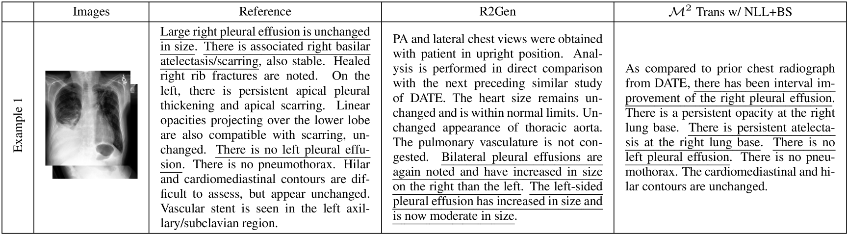
Figure 3: An example of radiology reports generated by R2Gen and by the proposed model with the optimization integrating BERTScore. Repeated sentences are removed from the example to improve readability.

5.2 Human Evaluation

We performed a human evaluation to further confirm whether the generated radiology reports are factually complete and consistent. Following prior studies of radiology report summarization Zhang et al. (2020b) and image captioning evaluation Vedantam et al. (2015), we designed a simple human evaluation task. Given a reference report (R) and two candidate model generated reports (C1, C2), two board-certified radiologists decided whether C1 or C2 is more factually similar to R. To consider cases when C1 and C2 are difficult to differentiate, we also prepared “No difference” as an answer. We sampled $100$ reports randomly from the test set of MIMIC-CXR for this evaluation. Since this evaluation is (financially) expensive and there has been no human evaluation between the baseline models, we selected R2Gen as the best previous model and $\mathcal{M}^{2}$ Trans w/ BS as the most simple proposed model, in order to be able to weakly infer that all of our proposed models are better than all of the baselines. Table 3 shows the result of the evaluation. The majority of the reports were labeled “No difference” but the proposed approach received three times as much preference as the baseline.

There are two main reasons why “No difference” was frequent in human evaluation. First, we found that a substantial portion of the examples were normal studies (no abnormal observations), which leads to generated reports of similar quality from both models. Second, in some reports with multiple abnormal observations, both models made mistakes on a subset of these observations, making it difficult to decide which model output was better.

$\mathcal{M}^{2}$ Trans w/ BS	R2Gen	No
Proposed (simple)	Chen et al. (2020)	difference
$36.5\%$	$12.0\%$	$51.5\%$

Table 3: The human evaluation result for randomly sampled $100$ reports from the test set of MIMIC-CXR by two board-certified radiologists.

5.3 Estimating Clinical Accuracy with Factual Rewards

The integrations of $\rm{fact}_{ENT}$ and $\rm{fact}_{ENTNLI}$ showed improvements in the clinical metrics. We further examined whether these rewards can be used to estimate the performance of the clinical metrics to see whether the proposed rewards can be used in an evaluation where a strong clinical information extraction system like CheXbert is not available. Table 4 shows Spearman correlations calculated on the generated reports of NLL+BS. $\mathrm{fact_{ENTNLI}}$ shows the strongest correlation with the clinical accuracy which aligns with the optimization where the best accuracy is obtained with NLL+ BS+$\mathrm{fact_{ENTNLI}}$. This correlation value is slightly lower than a Spearman correlation which Maynez et al. (2020) observed with NLI for the factual data ($0.264$). The result suggests the effectiveness of using the factual rewards to estimate the factual completeness and consistency of radiology reports, although the correlations are still limited, with some room for improvement.

Metric	$\rho$
BLEU4	$0.092$
CIDEr-D	$0.034$
BERTScore	$0.155$
$\mathrm{fact_{ENT}}$	$0.196$
$\mathrm{fact_{ENTNLI}}$	$\boldsymbol{0.255}$

Table 4: The Spearman correlations $\rho$ of NLG metrics and factual metrics against clinical accuracy. The strongest correlation among all metrics is shown is bold.

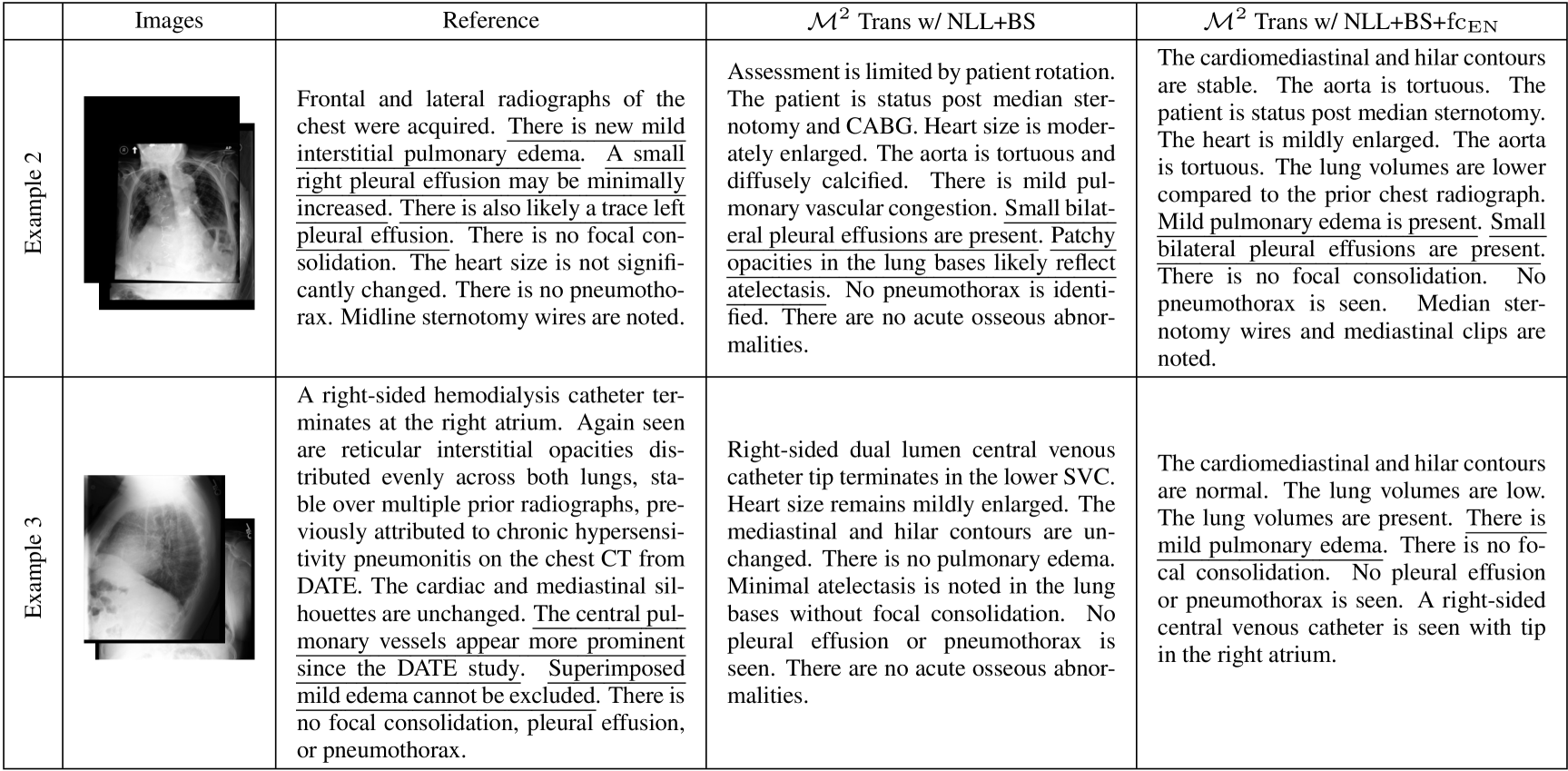
Figure 4: Examples of radiology reports generated by the proposed model with the optimization integrating BERTScore and $\mathrm{fact_{ENTNLI}}$. Repeated sentences are removed from the examples to improve readability.

5.4 Qualitative Analysis of Improved Clinical Completeness and Consistency

The evaluation with the clinically findings metrics showed improved generation performance by integrating BERTScore, $\rm{fact}_{ENT}$, and $\rm{fact}_{ENTNLI}$. As a qualitative analysis, we examined some of the generated reports to see the improvements. Example 1 in Figure 3 shows the improved factual completeness and consistency with BERTScore. The atelectasis is correctly generated and left plural effusion is correctly suppressed with NLL+BS. Example 2 in Figure 4 shows the improved factual completeness with $\mathrm{fact_{ENTNLI}}$. The edema is correctly generated and atelectasis is correctly suppressed with NLL+BS+$\mathrm{fc_{EN}}$. These examples reveal the strength of integrating the three metrics to generate factually complete and consistent reports.

Despite observing large improvements with our model in the clinical finding metrics evaluation, the model is still not complete and some typical factual errors can be found in their generated reports. For example, Example 3 in Figure 4 includes a comparison of an observation against a previous study as “…appear more prominent since …” in the reference but our model (or any previous models) can not capture this kind of comparison since the model is not designed to take account the past reports of a patient as input. Additionally, in this example, edema is mentioned with uncertainty as “cannot be excluded” in the reference but the generated report with $\rm{fact}_{ENTNLI}$ simply indicates it as “There is mild pulmonary edema”.

6 Conclusion

We proposed two new simple rewards and combined them with a semantic equivalence metric to improve image-to-text radiology report generation systems. The two new rewards make use of radiology domain entities extracted with a named entity recognizer and a weakly-supervised NLI to capture the factual completeness and consistency of the generated reports. We further presented a Transformer-based report generation system that directly optimizes these rewards with self-critical reinforcement learning. On two open datasets, we showed that our system generates reports that are more factually complete and consistent than the baselines and leads to reports with substantially higher scores in clinical metrics. The integration of entities and NLI to improve the factual completeness and consistency of generation is not restricted to the domain of radiology reports, and we predict that a similar approach might similarly improve other data-to-text tasks.

Appendix A Detail of Radiology NLI

A.1 Rules & Examples of Weakly-Supervised Radiology NLI

We prepared the $6$ rules (E1, N1–N4, and C1) to train the weakly-supervised radiology NLI. The rules are applied against sentence pairs consisting from premises ($s_{1}$) and hypotheses ($s_{2}$) to extract pairs that are in entailment, neutral, or contradiction relation.

Entailment Rule: E1

1. $s_{1}$ and $s_{2}$ are semantically similar.

2. The named entities (NE) of $s_{2}$ is a subset or equal to the named entities of $s_{1}$ as $\rm{NE}(\rm{s_{2}})\subseteq\rm{NE}(\rm{s_{1}})$.

We used BERTScore Zhang et al. (2020a) as a similarity metric and set the threshold to $sim(\rm{s_{1}},\rm{s_{2}})\geq 0.7$. The clinical model of Stanza Zhang et al. (2020c) is used to extract anatomy entities and observation entities. $s_{1}$ and $s_{2}$ are conditioned to be both negated or both non-negated. The negation is determined with a negation identifier or the existence of uncertain entity, using NegBio Peng et al. (2018) as the negation identifier and the clinical model of Stanza is used to extract uncertain entities. $s_{2}$ is further restricted to include at least $2$ entities as $|\rm{NE}(\rm{s_{2}})|\geq 2$. These similarity metric, named entity recognition model, and entity number restriction are used in the latter neutral and contradiction rules. The negation restriction is used in the neutral rules but is not used in the contradiction rule. The following is an example of a sentence pair that matches E1 with entities in bold:

$\boldsymbol{s_{1}}$

The heart is mildly enlarged.

$\boldsymbol{s_{2}}$

The heart appears again mild-to-moderately enlarged.

Neutral Rule 1: N1

1. $s_{1}$ and $s_{2}$ are semantically similar.

2. The named entities of $s_{1}$ is a subset of the named entities of $s_{2}$ as $\rm{NE}(\rm{s_{1}})\subsetneq\rm{NE}(\rm{s_{2}})$.

Since $s_{1}$ is a premise, this condition denotes that the counterpart hypothesis has entities that are not included in the premise. The following is an example of a sentence pair that matches N1 with entities in bold:

$\boldsymbol{s_{1}}$

There is no pulmonary edema or definite consolidation.

$\boldsymbol{s_{2}}$

There is no focal consolidation, pleural effusion, or pulmonary edema.

Neutral Rule 2: N2

1. The named entities of $s_{1}$ are equal to the named entities of $s_{2}$ as $\rm{NE}(\rm{s_{1}})=\rm{NE}(\rm{s_{2}})$.

2. The anatomy modifiers ($\rm{NE}_{mod}$) of $s_{1}$ include an antonym (ANT) of the anatomy modifier of $s_{2}$ as $\rm{NE}_{\rm mod}(s_{1})\cap ANT(\rm{NE}_{\rm mod}(s_{2}))\neq\emptyset$.

Anatomy modifiers are extracted with the clinical model of Stanza and antonyms are decided using WordNet Fellbaum (1998). Antonyms in anatomy modifiers are considered in this rule to differentiate experessions like left vs right and upper vs lower. The following is an example of a sentence pair that matches N2 with antonyms in bold:

$\boldsymbol{s_{1}}$

Moreover, a small left pleural effusion has newly occurred.

$\boldsymbol{s_{2}}$

Small right pleural effusion has worsened.

Neutral Rule 3: N3

1. The named entity types ($\rm{NE}_{type}$) of $s_{1}$ are equal to the named entity types of $s_{2}$ as $\rm{NE}_{\rm type}(\rm{s_{1}})=\rm{NE}_{\rm type}(\rm{s_{2}})$.

2. The named entities of $s_{1}$ is different from the named entities of $s_{2}$ as $\rm{NE}(\rm{s_{1}})\cap\rm{NE}(\rm{s_{2}})=\emptyset$.

Specific entity types that we used are anatomy and observation. This rule ensures that $s_{1}$ and $s_{2}$ have related but different entities in same types. The following is an example of a sentence pair that matches N3 with entities in bold:

$\boldsymbol{s_{1}}$

There is minimal bilateral lower lobe atelectasis.

$\boldsymbol{s_{2}}$

The cardiac silhouette is moderately enlarged.

Neutral Rule 4: N4

1. The named entities of $s_{1}$ are equal to the named entities of $s_{2}$ as $\rm{NE}(\rm{s_{1}})=\rm{NE}(\rm{s_{2}})$.

2. $s_{1}$ and $s_{2}$ include observation keywords (KEY) that belong to different groups as $\rm{KEY}(s_{1})\neq\rm{KEY}(s_{2})$.

The groups of observation keywords are setup following the observation keywords of CheXpert labeler Irvin et al. (2019). Specifically, ${\rm G1}=\{normal,unremarkable\}$, ${\rm G2}=\{stable,unchanged\}$, and ${\rm G3}=\{clear\}$ are used to determine words included in different groups as neutral relation. The following is an example of a sentence pair that matches N4 with keywords in bold:

$\boldsymbol{s_{1}}$

Normal cardiomediastinal silhouette.

$\boldsymbol{s_{2}}$

Cardiomediastinal silhouette is unchanged.

Contradiction Rule: C1

1. The named entities of $s_{1}$ is a subset or equal to the named entities of $s_{2}$ as $\rm{NE}(\rm{s_{2}})\subseteq\rm{NE}(\rm{s_{1}})$.

2. $s_{1}$ or $s_{2}$ is a negated sentence.

Negation is determined with the same approach as E1. The following is an example of a sentence pair that matches C1 with entities in bold:

$\boldsymbol{s_{1}}$

There are also small bilateral pleural effusions.

$\boldsymbol{s_{2}}$

No pleural effusions.

A.2 Validation and Test Datasets of Radiology NLI

We sampled $480$ sentence pairs that satisfy the following conditions from the validation section of MIMIC-CXR:

1. Two sentences ($s_{1}$ and $s_{2}$) have ${\rm BERTScore(s_{1},s_{2})}\geq 0.5$.

2. MedNLI labels are equally distributed over three labels: entailment, neutral, and contradiction.

These conditions are introduced to reduce neutral pairs since most pairs will be neutral with random sampling. The sampled pairs are annotated twice swapping its premise and hypothesis by two experts: one medical expert and one NLP expert. For pairs that the two annotators disagreed, its labels are decided by a discussion with one additional NLP expert. The resulting $960$ bidirectional pairs are splitted in half resulting in $480$ pairs for a validation set and $480$ pairs for a test set.

A.3 Configuration of Radiology NLI Model

We used bert-base-uncased as a pre-trained BERT model and further fine-tuned it on MIMIC-III Johnson et al. (2016) radiology reports with a masked language modeling loss for $8$ epochs. The model is further optimized on the training data with a classification negative log likelihood loss. We used Adam Kingma and Ba (2015) as an optimization method with $\beta_{1}=0.9$, $\beta_{2}=0.999$, batch size of $16$, and the gradient clipping norm of $5.0$. The learning rate is set to $lr=1e^{-5}$ by running a preliminary experiment with $lr=\{1e^{-5},2e^{-5}\}$. The model is optimized for the maximum of $20$ epochs and a validation accuracy is used to decide a model checkpoint that is used to evaluate the test set. We trained the model with a single Nvidia Titan XP taking approximately $2$ hours to complete $20$ epochs.

Appendix B Configurations of Radiology Report Generation Models

B.1 $\boldsymbol{\mathcal{M}^{2}}$ Trans

We used DenseNet-121 Huang et al. (2017) as a CNN image feature extractor and pre-trained it on CheXpert dataset with the $14$-class classification setting. We used GloVe Pennington et al. (2014) to pre-train text embeddings and the pre-trainings were done on a training set with the embedding size of $512$. The parameters of the model is set up to the dimensionality of $512$, the number of heads to $8$, and the number of memory vector to $40$. We set the number of Transformer layer to $n_{layer}=1$ by running a preliminary experiment with $n_{layer}=\{1,2,3\}$. The model is first trained against NLL loss using the learning rate scheduler of Transformer Devlin et al. (2019) with the warm-up steps of $20000$ and is further optimized with a joint loss with the fixed learning rate of $5e^{-6}$. Adam is used as an optimization method with $\beta_{1}=0.9$ and $\beta_{2}=0.999$. The batch size is set to $48$ for NLL loss and $24$ for the joint losses. For $\lambda_{*}$, we first swept the optimal value of $\lambda_{1}$ from $\{0.03,0.02,0.01,0.001\}$ using the development set. We have restricted $\lambda_{2}$ and $\lambda_{3}$ to have equal values in our experiments and constrined that all $\lambda_{*}$ values sum up to $1.0$. The model is trained with NLL loss for $32$ epochs and further trained for $32$ epochs with a joint loss. Beam search with the beam size of $4$ is used to decode texts when evaluating the model against a validation set or a test set. We trained the model with a single Nvidia Titan XP taking approximately $10$ days to complete its optimization.

		MIMIC-CXR				Open-i
Observation (# MIMIC-CXR / # Open-i)		R2Gen	NLL + BS	NLL + BS + $\mathrm{fc_{E}}$	NLL + BS + $\mathrm{fc_{EN}}$	R2Gen	NLL + BS	NLL + BS + $\mathrm{fc_{E}}$	NLL + BS + $\mathrm{fc_{EN}}$
	P	$41.2$	$46.3$	$46.3$	$50.3$	$27.0$	$47.7$	$44.0$	$48.7$
Micro Average	R	$29.8$	$67.5$	$73.2$	$65.1$	$17.3$	$46.6$	$53.5$	$46.9$
($2713$ / $654$)	$\mathrm{F}_{1}$	$34.6$	$54.9$	$56.7$	$56.7$	$21.1$	$47.2$	$48.3$	$47.8$
	acc.	$73.9$	$74.4$	$74.2$	$77.1$	$94.9$	$95.9$	$95.5$	$96.0$
	P	$35.4$	$39.9$	$37.9$	$40.6$	$35.6$	$44.0$	$35.8$	$39.4$
Atelectasis	R	$27.8$	$67.4$	$80.5$	$76.2$	$7.4$	$35.6$	$47.7$	$45.4$
($604$ / $216$)	$\mathrm{F}_{1}$	$31.1$	$50.2$	$51.6$	$53.0$	$12.3$	$39.4$	$40.9$	$42.2$
	acc.	$68.3$	$65.5$	$61.1$	$65.2$	$93.1$	$92.9$	$91.1$	$91.9$
	P	$32.4$	$35.8$	$34.3$	$37.5$	$24.5$	$56.6$	$57.3$	$60.0$
Cardiomegaly	R	$53.5$	$73.3$	$81.3$	$61.3$	$33.8$	$55.6$	$55.6$	$46.7$
($535$ / $225$)	$\mathrm{F}_{1}$	$40.4$	$48.1$	$48.2$	$46.6$	$28.4$	$56.1$	$56.4$	$52.5$
	acc.	$64.0$	$63.9$	$60.2$	$67.9$	$88.5$	$94.1$	$94.2$	$94.3$
	P	$14.3$	$10.5$	$19.6$	$19.2$	$0.0$	$10.9$	$15.2$	$14.3$
Consolidation	R	$7.0$	$18.5$	$5.7$	$3.2$	$0.0$	$26.3$	$26.3$	$5.3$
($157$ / $19$)	$\mathrm{F}_{1}$	$9.4$	$13.4$	$8.9$	$5.5$	$0.0$	$15.4$	$19.2$	$7.7$
	acc.	$91.0$	$84.0$	$92.1$	$92.6$	$99.0$	$98.4$	$98.7$	$99.3$
	P	$55.3$	$59.7$	$56.0$	$65.6$	$10.0$	$39.0$	$30.9$	$41.4$
Edema	R	$24.3$	$59.2$	$69.9$	$52.7$	$4.0$	$30.7$	$50.7$	$32.0$
($645$ / $75$)	$\mathrm{F}_{1}$	$33.8$	$59.5$	$62.2$	$58.5$	$5.7$	$34.3$	$38.4$	$36.1$
	acc.	$73.8$	$77.8$	$76.6$	$79.4$	$97.0$	$97.4$	$96.3$	$97.5$
	P	$76.2$	$67.2$	$68.2$	$65.9$	$85.7$	$54.3$	$59.4$	$56.0$
Pleural Effusion	R	$24.1$	$80.6$	$78.5$	$82.0$	$15.1$	$63.0$	$66.4$	$66.4$
($772$ / $119$)	$\mathrm{F}_{1}$	$36.6$	$73.3$	$73.0$	$73.1$	$25.7$	$58.4$	$62.7$	$60.8$
	acc.	$72.6$	$80.7$	$80.9$	$80.1$	$96.9$	$96.8$	$97.2$	$96.9$

Table 5: The detailed results of R2Gen, $\mathcal{M}^{2}$ Trans w/ BS, $\mathcal{M}^{2}$ Trans w/ BS+$\mathrm{{fc}_{E}}$, and $\mathcal{M}^{2}$ Trans w/ BS+$\mathrm{{fc}_{EN}}$ for the $5$ observations. P is precision, R is recall, and acc. is accuracy. #MIMIC- CXR and #Open-i are the numbers of times that a corresponding observation has appeared as positive in the test set of MIMIC-CXR and Open-i, respectively.

		MIMIC-CXR				Open-i
Observation (# MIMIC-CXR / # Open-i)		R2Gen	NLL + BS	NLL + BS + $\mathrm{fc_{E}}$	NLL + BS + $\mathrm{fc_{EN}}$	R2Gen	NLL + BS	NLL + BS + $\mathrm{fc_{E}}$	NLL + BS + $\mathrm{fc_{EN}}$
	P	$37.6$	$46.0$	$46.0$	$49.9$	$16.7$	$46.3$	$42.7$	$47.8$
Micro Average	R	$29.1$	$67.2$	$72.9$	$64.6$	$17.1$	$45.8$	$52.5$	$46.3$
($2713$ / $654$)	$\mathrm{F}_{1}$	$32.8$	$54.6$	$56.4$	$56.3$	$16.9$	$46.1$	$47.1$	$47.0$
	acc.	$74.6$	$74.2$	$74.0$	$76.8$	$93.4$	$95.8$	$95.4$	$95.9$
	P	$35.6$	$39.9$	$37.8$	$40.6$	$33.3$	$42.9$	$34.7$	$38.2$
Atelectasis	R	$23.9$	$67.6$	$80.6$	$76.4$	$7.1$	$35.4$	$47.2$	$44.8$
($604$ / $216$)	$\mathrm{F}_{1}$	$28.6$	$50.2$	$51.5$	$53.0$	$11.7$	$38.8$	$40.0$	$41.2$
	acc.	$72.1$	$65.6$	$61.1$	$65.3$	$93.2$	$92.9$	$91.0$	$91.9$
	P	$28.6$	$36.1$	$34.6$	$37.6$	$20.4$	$55.2$	$55.5$	$60.0$
Cardiomegaly	R	$49.2$	$72.8$	$81.1$	$60.5$	$31.3$	$53.5$	$53.0$	$45.7$
($535$ / $225$)	$\mathrm{F}_{1}$	$36.2$	$48.2$	$48.5$	$46.4$	$24.7$	$54.3$	$54.2$	$51.9$
	acc.	$63.0$	$63.8$	$60.0$	$67.6$	$86.8$	$93.8$	$93.8$	$94.2$
	P	$10.7$	$10.5$	$19.6$	$19.2$	$1.1$	$10.9$	$14.7$	$14.3$
Consolidation	R	$9.4$	$17.8$	$5.5$	$3.1$	$10.5$	$26.3$	$26.3$	$5.3$
($157$ / $19$)	$\mathrm{F}_{1}$	$10.0$	$13.2$	$8.6$	$5.3$	$2.0$	$15.4$	$18.9$	$7.7$
	acc.	$88.4$	$83.7$	$91.9$	$92.4$	$94.0$	$98.4$	$98.7$	$99.3$
	P	$49.0$	$58.7$	$54.9$	$64.3$	$5.8$	$35.0$	$30.1$	$39.7$
Edema	R	$29.1$	$59.0$	$69.5$	$52.3$	$4.1$	$28.8$	$50.7$	$31.5$
($645$ / $75$)	$\mathrm{F}_{1}$	$36.5$	$58.8$	$61.4$	$57.7$	$4.8$	$31.6$	$37.8$	$35.1$
	acc.	$74.5$	$77.6$	$76.2$	$79.2$	$96.4$	$97.3$	$96.3$	$97.5$
	P	$75.6$	$66.5$	$67.6$	$65.2$	$63.3$	$53.2$	$57.5$	$54.6$
Pleural Effusion	R	$23.4$	$80.3$	$78.2$	$81.6$	$16.4$	$63.8$	$66.4$	$66.4$
($772$ / $119$)	$\mathrm{F}_{1}$	$35.8$	$72.7$	$72.5$	$72.5$	$26.0$	$58.0$	$61.6$	$59.9$
	acc.	$75.1$	$80.3$	$80.6$	$79.8$	$96.8$	$96.8$	$97.1$	$96.9$

Table 6: The detailed results of R2Gen, $\mathcal{M}^{2}$ Trans w/ BS, $\mathcal{M}^{2}$ Trans w/ BS+$\mathrm{{fc}_{E}}$, and $\mathcal{M}^{2}$ Trans w/ BS+$\mathrm{{fc}_{EN}}$ for the $5$ observations evaluated with CheXpert instead of CheXbert.

		MIMIC-CXR				Open-i
Observation (# MIMIC-CXR / # Open-i)		R2Gen	NLL + BS	NLL + BS + $\mathrm{fc_{E}}$	NLL + BS + $\mathrm{fc_{EN}}$	R2Gen	NLL + BS	NLL + BS + $\mathrm{fc_{E}}$	NLL + BS + $\mathrm{fc_{EN}}$
	P	$4.4$	$5.1$	$4.8$	$4.6$	$3.8$	$0.7$	$2.0$	$4.0$
Enlarged Cardiomediastinum	R	$19.8$	$50.5$	$19.8$	$47.7$	$16.7$	$4.2$	$4.2$	$20.8$
($111$ / $24$)	$\mathrm{F}_{1}$	$7.1$	$9.3$	$7.7$	$8.4$	$6.3$	$1.2$	$2.7$	$6.7$
	acc.	$75.6$	$53.4$	$77.5$	$50.6$	$96.4$	$95.1$	$97.8$	$95.8$
	P	$0.0$	$40.0$	$10.7$	$26.1$	$0.0$	$0.0$	$0.0$	$3.1$
Fracture	R	$0.0$	$3.6$	$5.4$	$10.7$	$0.0$	$0.0$	$0.0$	$2.3$
($56$ / $43$)	$\mathrm{F}_{1}$	$0.0$	$6.6$	$7.1$	$15.2$	$0.0$	$0.0$	$0.0$	$2.7$
	acc.	$97.6$	$97.6$	$96.7$	$97.1$	$98.7$	$98.6$	$98.1$	$97.8$
	P	$37.5$	$33.3$	$22.2$	$44.4$	$25.0$	$0.0$	$0.0$	$66.7$
Lung Lesion	R	$3.1$	$1.0$	$2.1$	$4.1$	$1.1$	$0.0$	$0.0$	$4.5$
($97$ / $89$)	$\mathrm{F}_{1}$	$5.7$	$2.0$	$3.8$	$7.5$	$2.2$	$0.0$	$0.0$	$8.4$
	acc.	$95.8$	$95.8$	$95.7$	$95.8$	$97.3$	$97.3$	$97.3$	$97.4$
	P	$44.5$	$48.8$	$53.5$	$54.9$	$43.1$	$50.5$	$57.8$	$41.1$
Lung Opacity	R	$29.9$	$41.6$	$10.4$	$26.6$	$8.1$	$29.1$	$7.6$	$22.1$
($798$ / $344$)	$\mathrm{F}_{1}$	$35.8$	$44.9$	$17.4$	$35.8$	$13.7$	$36.9$	$13.4$	$28.7$
	acc.	$63.5$	$65.3$	$66.5$	$67.6$	$89.4$	$89.7$	$89.9$	$88.7$
	P	$31.4$	$44.4$	$49.8$	$48.8$	$78.1$	$80.8$	$82.1$	$81.7$
No Finding	R	$43.9$	$35.9$	$41.7$	$39.9$	$84.1$	$93.4$	$91.5$	$88.4$
($396$ / $2319$)	$\mathrm{F}_{1}$	$36.6$	$39.7$	$45.4$	$43.9$	$81.0$	$86.6$	$86.5$	$84.9$
	acc.	$74.4$	$81.6$	$83.1$	$82.8$	$72.6$	$80.0$	$80.2$	$78.2$
	P	$0.0$	$0.0$	$0.0$	$0.0$	$0.0$	$0.0$	$0.0$	$0.0$
Pleural Other	R	$0.0$	$0.0$	$0.0$	$0.0$	$0.0$	$0.0$	$0.0$	$0.0$
($39$ / $29$)	$\mathrm{F}_{1}$	$0.0$	$0.0$	$0.0$	$0.0$	$0.0$	$0.0$	$0.0$	$0.0$
	acc.	$98.1$	$98.3$	$98.3$	$98.3$	$99.1$	$99.1$	$99.1$	$99.1$
	P	$42.1$	$62.7$	$62.1$	$0.0$	$27.6$	$31.3$	$38.6$	$0.0$
Pneumonia	R	$15.8$	$16.3$	$17.0$	$0.0$	$7.3$	$19.3$	$24.8$	$0.0$
($424$ / $109$)	$\mathrm{F}_{1}$	$23.0$	$25.8$	$26.7$	$0.0$	$11.6$	$23.9$	$30.2$	$0.0$
	acc.	$80.9$	$83.1$	$83.1$	$81.9$	$96.3$	$96.0$	$96.3$	$96.7$
	P	$60.0$	$28.7$	$37.0$	$50.0$	$100.0$	$40.0$	$0.0$	$100.0$
Pneumothorax	R	$3.8$	$34.6$	$12.8$	$10.3$	$6.7$	$13.3$	$0.0$	$13.3$
($78$ / $15$)	$\mathrm{F}_{1}$	$7.2$	$31.4$	$19.0$	$17.0$	$12.5$	$20.0$	$0.0$	$23.5$
	acc.	$96.7$	$95.0$	$96.4$	$96.7$	$99.6$	$99.5$	$99.6$	$99.6$
	P	$52.2$	$50.8$	$53.2$	$49.0$	$10.0$	$16.2$	$19.7$	$13.1$
Support Devices	R	$68.9$	$83.5$	$78.7$	$89.7$	$12.2$	$43.9$	$36.6$	$56.1$
($624$ / $41$)	$\mathrm{F}_{1}$	$59.4$	$63.2$	$63.5$	$63.3$	$11.0$	$23.7$	$25.6$	$21.3$
	acc.	$75.0$	$74.1$	$75.9$	$72.4$	$97.6$	$96.5$	$97.4$	$94.9$

Table 7: The detailed results of R2Gen, $\mathcal{M}^{2}$ Trans w/ BS, $\mathcal{M}^{2}$ Trans w/ BS+$\mathrm{{fc}_{E}}$, and $\mathcal{M}^{2}$ Trans w/ BS+$\mathrm{{fc}_{EN}}$ for the remaining $9$ observations.

B.2 TieNet

We used ResNet-50 as a CNN image feature extractor with default ImageNet pre-trained weights. We used GloVe to pre-train text embeddings with the same configuration as $\mathcal{M}^{2}$ Trans. The parameters of the model is set up to the LSTM dimension of $256$ and the number of global attentions to $5$. The combination of NLL loss and the multi-label classification loss is used as its joint loss with the balance parameter $\alpha=0.85$. The model is trained against the joint loss using a linear rate scheduler with the initial learning rate of $1e^{-4}$ and the multiplication of $0.5$ per $8$ epochs. The batch size is set to $32$ and the model is trained with the joint loss for $32$ epochs. Adam is used as an optimization method with $\beta_{1}=0.9$ and $\beta_{2}=0.999$. Beam search with the beam size of $4$ is used to decode texts. We trained the model with a single Nvidia Titan XP taking approximately $2$ days to complete its optimization.

B.3 $\boldsymbol{\mathrm{CNN}}$-$\boldsymbol{\mathrm{RNN^{2}}}$

We used DenseNet-121 as a CNN image feature extractor with default ImageNet pre-trained weights. We used GloVe to pre-train text embeddings with the same configuration as $\mathcal{M}^{2}$ Trans. The parameters of the model is set up to the LSTM dimension of $256$. We modified an information extraction system from CheXpert to CheXbert to improve the training speed of this model. The combination of CIDEr and Clinically Coherent Reward is used as its joint loss with the balance parameter $\lambda=10.0$. The model is first trained against NLL loss using a linear rate scheduler with the initial learning rate of $1e^{-4}$ and the multiplication of $0.5$ per $8$ epochs. The model is further optimized with the joint loss with the fixed learning rate of $5e^{-6}$. Adam is used as an optimization method with $\beta_{1}=0.9$ and $\beta_{2}=0.999$. The batch size is set to $32$ for the NLL loss and $24$ for the joint losses. The model is trained with NLL loss for $32$ epochs and further trained for $32$ epochs with the joint loss. Beam search with the beam size of $4$ is used to decode texts. We trained the model with a single Nvidia Titan XP taking approximately $11$ days to complete its optimization.

Appendix C Detailed Result of Clinical Metrics

Table 5 shows the detailed results of the clinical metrics for R2Gen, $\mathcal{M}^{2}$ Trans w/ BS, $\mathcal{M}^{2}$ Trans w/ BS+$\mathrm{{fc}_{E}}$, and $\mathcal{M}^{2}$ Trans w/ BS+$\mathrm{{fc}_{EN}}$. In most cases, the best $\mathrm{F}_{1}$ scores are observed in the cases when $\mathrm{fact_{ENT}}$ or $\mathrm{fact_{ENTNLI}}$ is included in the joint losses. Consolidation is one exception where the best precisions, recalls, and $\mathrm{F}_{1}$ scores vary among the joint losses. We assume this is due to the infrequent appearance of consolidation in both MIMIC-CXR and Open-i. For comparison against some past studies, we show the detailed results when CheXpert is used instead of CheXbert in Table 6. Since CheXbert is more or equally accurate for most observations than CheXpert, the scores in Table 6 follow similar trends against ones in Table 5. Table 7 shows the detailed results for the $9$ remaining observations that are defined in CheXpert. Note that many of these observations are infrequent and have relatively weaker and unstable extraction performances compared to the $5$ observations in Table 5.

References

- Ben Abacha et al. (2019) Asma Ben Abacha, Chaitanya Shivade, and Dina Demner-Fushman. 2019. Overview of the MEDIQA 2019 shared task on textual inference, question entailment and question answering. In Proceedings of the 18th BioNLP Workshop and Shared Task, pages 370–379.
- Boag et al. (2020) William Boag, Tzu-Ming Harry Hsu, Matthew Mcdermott, Gabriela Berner, Emily Alesentzer, and Peter Szolovits. 2020. Baselines for Chest X-Ray Report Generation. In Proceedings of the Machine Learning for Health NeurIPS Workshop, volume 116, pages 126–140.
- Chen et al. (2020) Zhihong Chen, Yan Song, Tsung-Hui Chang, and Xiang Wan. 2020. Generating radiology reports via memory-driven transformer. In Proceedings of The 2020 Conference on Empirical Methods in Natural Language Processing, pages 1439–1449.
- Cornia et al. (2020) Marcella Cornia, Matteo Stefanini, Lorenzo Baraldi, and Rita Cucchiara. 2020. Meshed-Memory Transformer for Image Captioning. In Proceedings of the IEEE/CVF Conference on Computer Vision and Pattern Recognition, pages 10575–10584.
- Demner-Fushman et al. (2012) Dina Demner-Fushman, Samee Antani, Simpsonl Matthew, and George R. Thoma. 2012. Design and development of a multimodal biomedical information retrieval system. Journal of Computing Science and Engineering, 6(2):168–177.
- Devlin et al. (2019) Jacob Devlin, Ming-Wei Chang, Kenton Lee, and Kristina Toutanova. 2019. BERT: Pre-training of deep bidirectional transformers for language understanding. In Proceedings of the 2019 Conference of the North American Chapter of the Association for Computational Linguistics: Human Language Technologies, Volume 1 (Long and Short Papers), pages 4171–4186.
- Durmus et al. (2020) Esin Durmus, He He, and Mona Diab. 2020. FEQA: A question answering evaluation framework for faithfulness assessment in abstractive summarization. In Proceedings of the 58th Annual Meeting of the Association for Computational Linguistics, pages 5055–5070.
- Falke et al. (2019) Tobias Falke, Leonardo F. R. Ribeiro, Prasetya Ajie Utama, Ido Dagan, and Iryna Gurevych. 2019. Ranking generated summaries by correctness: An interesting but challenging application for natural language inference. In Proceedings of the 57th Annual Meeting of the Association for Computational Linguistics, pages 2214–2220.
- Fellbaum (1998) Christiane Fellbaum, editor. 1998. WordNet: A Lexical Database for English. MIT Press.
- Guo et al. (2020) Longteng Guo, Jing Liu, Xinxin Zhu, Peng Yao, Shichen Lu, and Hanqing Lu. 2020. Normalized and geometry-aware self-attention network for image captioning. In IEEE/CVF Conference on Computer Vision and Pattern Recognition, pages 10324–10333.
- Herdade et al. (2019) Simao Herdade, Armin Kappeler, Kofi Boakye, and Joao Soares. 2019. Image captioning: Transforming objects into words. In Advances in Neural Information Processing, volume 32, pages 11137–11147.
- Huang et al. (2017) Gao Huang, Zhuang Liu, Laurens van der Maaten, and Kilian Q. Weinberger. 2017. Densely connected convolutional networks. In Proceedings of the IEEE Conference on Computer Vision and Pattern Recognition, pages 2261–2269.
- Irvin et al. (2019) Jeremy Irvin, Pranav Rajpurkar, Michael Ko, Yifan Yu, Silviana Ciurea-Ilcus, Chris Chute, Henrik Marklund, Behzad Haghgoo, Robyn L. Ball, Katie S. Shpanskaya, Jayne Seekins, David A. Mong, Safwan S. Halabi, Jesse K. Sandberg, Ricky Jones, David B. Larson, Curtis P. Langlotz, Bhavik N. Patel, Matthew P. Lungren, and Andrew Y. Ng. 2019. CheXpert: A large chest radiograph dataset with uncertainty labels and expert comparison. In The Thirty-Third AAAI Conference on Artificial Intelligence, volume 33, pages 590–597.
- Jing et al. (2019) Baoyu Jing, Zeya Wang, and Eric Xing. 2019. Show, describe and conclude: On exploiting the structure information of chest x-ray reports. In Proceedings of the 57th Annual Meeting of the Association for Computational Linguistics, pages 6570–6580.
- Jing et al. (2018) Baoyu Jing, Pengtao Xie, and Eric Xing. 2018. On the automatic generation of medical imaging reports. In Proceedings of the 56th Annual Meeting of the Association for Computational Linguistics (Volume 1: Long Papers), pages 2577–2586.
- Johnson et al. (2019) Alistair E. W. Johnson, Tom J. Pollard, Seth J. Berkowitz, Nathaniel R. Greenbaum, Matthew P. Lungren, Chih-ying Deng, Roger G. Mark, and Steven Horng. 2019. MIMIC-CXR, a de-identified publicly available database of chest radiographs with free-text reports. Scientific Data, 6(317).
- Johnson et al. (2016) Alistair E. W. Johnson, Tom J. Pollard, Lu Shen, Li-wei H. Lehman, Mengling Feng, Mohammad Ghassemi, Benjamin Moody, Peter Szolovits, Leo Anthony Celi, and Roger G. Mark. 2016. MIMIC-III, a freely accessible critical care database. Scientific Data, 3(16035).
- Kahn et al. (2009) Charles E. Kahn, Curtis P. Langlotz, Elizabeth S. Burnside, John A. Carrino, David S. Channin, David M. Hovsepian, and Daniel L. Rubin. 2009. Toward best practices in radiology reporting. Radiology, 252(3):852–856.
- Kingma and Ba (2015) Diederik P. Kingma and Jimmy Ba. 2015. Adam: A method for stochastic optimization. In International Conference for Learning Representations.
- Kryściński et al. (2020) Wojciech Kryściński, Bryan McCann, Caiming Xiong, and Richard Socher. 2020. Evaluating the factual consistency of abstractive text summarization. In Proceedings of the 2020 Conference on Empirical Methods in Natural Language Processing, pages 9332–9346.
- Li et al. (2018) Christy Yuan Li, Xiaodan Liang, Zhiting Hu, and Eric P Xing. 2018. Hybrid retrieval-generation reinforced agent for medical image report generation. In Advances in Neural Information Processing, volume 31, pages 1530–1540.
- Li et al. (2019) Guang Li, Linchao Zhu, Ping Liu, and Yi Yang. 2019. Entangled transformer for image captioning. In Proceedings of the IEEE/CVF International Conference on Computer Vision, pages 8927–8936.
- Liu et al. (2019) Guanxiong Liu, Tzu-Ming Harry Hsu, Matthew McDermott, Willie Boag, Wei-Hung Weng, Peter Szolovits, and Marzyeh Ghassemi. 2019. Clinically accurate chest x-ray report generation. In Proceedings of the 4th Machine Learning for Healthcare Conference, volume 106, pages 249–269.
- Matsumaru et al. (2020) Kazuki Matsumaru, Sho Takase, and Naoaki Okazaki. 2020. Improving truthfulness of headline generation. In Proceedings of the 58th Annual Meeting of the Association for Computational Linguistics, pages 1335–1346.
- Maynez et al. (2020) Joshua Maynez, Shashi Narayan, Bernd Bohnet, and Ryan McDonald. 2020. On faithfulness and factuality in abstractive summarization. In Proceedings of the 58th Annual Meeting of the Association for Computational Linguistics, pages 1906–1919.
- Pan et al. (2020) Yingwei Pan, Ting Yao, Yehao Li, and Tao Mei. 2020. X-linear attention networks for image captioning. In Proceedings of the IEEE/CVF Conference on Computer Vision and Pattern Recognition, pages 10968–10977.
- Papineni et al. (2002) Kishore Papineni, Salim Roukos, Todd Ward, and Wei-Jing Zhu. 2002. Bleu: a method for automatic evaluation of machine translation. In Proceedings of the 40th Annual Meeting of the Association for Computational Linguistics, pages 311–318.
- Paulus et al. (2018) Romain Paulus, Caiming Xiong, and Richard Socher. 2018. A deep reinforced model for abstractive summarization. In International Conference on Learning Representations.
- Peng et al. (2018) Yifan Peng, Xiaosong Wang, Le Lu, Mohammadhadi Bagheri, Ronald Summers, and Zhiyong Lu. 2018. Negbio: a high-performance tool for negation and uncertainty detection in radiology reports. In AMIA 2018 Informatics Summit.
- Pennington et al. (2014) Jeffrey Pennington, Richard Socher, and Christopher Manning. 2014. GloVe: Global vectors for word representation. In Proceedings of the 2014 Conference on Empirical Methods in Natural Language Processing, pages 1532–1543.
- Qi et al. (2020) Peng Qi, Yuhao Zhang, Yuhui Zhang, Jason Bolton, and Christopher D. Manning. 2020. Stanza: A python natural language processing toolkit for many human languages. In Proceedings of the 58th Annual Meeting of the Association for Computational Linguistics: System Demonstrations, pages 101–108.
- Ranzato et al. (2016) Marc’Aurelio Ranzato, Sumit Chopra, Michael Auli, and Wojciech Zaremba. 2016. Sequence level training with recurrent neural networks. In International Conference on Learning Representations.
- Rennie et al. (2017) Steven J. Rennie, Etienne Marcheret, Youssef Mroueh, Jerret Ross, and Vaibhava Goel. 2017. Self-critical sequence training for image captioning. In Proceedings of the IEEE Conference on Computer Vision and Pattern Recognition, pages 1179–1195.
- Romanov and Shivade (2018) Alexey Romanov and Chaitanya Shivade. 2018. Lessons from natural language inference in the clinical domain. In Proceedings of the 2018 Conference on Empirical Methods in Natural Language Processing, pages 1586–1596.
- Smit et al. (2020) Akshay Smit, Saahil Jain, Pranav Rajpurkar, Anuj Pareek, Andrew Ng, and Matthew Lungren. 2020. Combining automatic labelers and expert annotations for accurate radiology report labeling using BERT. In Proceedings of the 2020 Conference on Empirical Methods in Natural Language Processing, pages 1500–1519.
- Vaswani et al. (2017) Ashish Vaswani, Noam Shazeer, Niki Parmar, Jakob Uszkoreit, Llion Jones, Aidan N Gomez, Łukasz Kaiser, and Illia Polosukhin. 2017. Attention is all you need. In Advances in neural information processing systems, volume 30, pages 5998–6008.
- Vedantam et al. (2015) Ramakrishna Vedantam, C. Lawrence Zitnick, and Devi Parikh. 2015. CIDEr: Consensus-based image description evaluation. In Proceedings of the IEEE Conference on Computer Vision and Pattern Recognition, pages 4566–4575.
- Vinyals et al. (2015) Oriol Vinyals, Alexander Toshev, Samy Bengio, and Dumitru Erhan. 2015. Show and tell: A neural image caption generator. In Proceedings of the IEEE Conference on Computer Vision and Pattern Recognition, pages 3156–3164.
- Wang et al. (2020a) Alex Wang, Kyunghyun Cho, and Mike Lewis. 2020a. Asking and answering questions to evaluate the factual consistency of summaries. In Proceedings of the 58th Annual Meeting of the Association for Computational Linguistics, pages 5008–5020.
- Wang et al. (2018) Xiaosong Wang, Yifan Peng, Le Lu, Zhiyong Lu, and Ronald M. Summers. 2018. TieNet: Text-image embedding network for common thorax disease classification and reporting in chest x-rays. In Proceedings of the IEEE Conference on Computer Vision and Pattern Recognition, pages 9049–9058.
- Wang et al. (2020b) Zhenyi Wang, Xiaoyang Wang, Bang An, Dong Yu, and Changyou Chen. 2020b. Towards faithful neural table-to-text generation with content-matching constraints. In Proceedings of the 58th Annual Meeting of the Association for Computational Linguistics, pages 1072–1086.
- Welleck et al. (2019) Sean Welleck, Jason Weston, Arthur Szlam, and Kyunghyun Cho. 2019. Dialogue natural language inference. In Proceedings of the 57th Annual Meeting of the Association for Computational Linguistics, pages 3731–3741.
- Williams and Zipser (1989) Ronald J Williams and David Zipser. 1989. A learning algorithm for continually running fully recurrent neural networks. Neural computation, 1(2):270–280.
- Wu et al. (2019) Zhaofeng Wu, Yan Song, Sicong Huang, Yuanhe Tian, and Fei Xia. 2019. WTMED at MEDIQA 2019: A hybrid approach to biomedical natural language inference. In Proceedings of the 18th BioNLP Workshop and Shared Task, pages 415–426.
- Yuan et al. (2019) Jianbo Yuan, Haofu Liao, Rui Luo, and Jiebo Luo. 2019. Automatic radiology report generation based on multi-view image fusion and medical concept enrichment. In Medical Image Computing and Computer Assisted Intervention, pages 721–729.
- Zhang et al. (2020a) Tianyi Zhang, Varsha Kishore, Felix Wu, Kilian Q. Weinberger, and Yoav Artzi. 2020a. BERTScore: Evaluating text generation with BERT. In International Conference on Learning Representations.
- Zhang et al. (2020b) Yuhao Zhang, Derek Merck, Emily Tsai, Christopher D. Manning, and Curtis Langlotz. 2020b. Optimizing the factual correctness of a summary: A study of summarizing radiology reports. In Proceedings of the 58th Annual Meeting of the Association for Computational Linguistics, pages 5108–5120.
- Zhang et al. (2020c) Yuhao Zhang, Yuhui Zhang, Peng Qi, Christopher D. Manning, and Curtis P. Langlotz. 2020c. Biomedical and clinical English model packages in the Stanza Python NLP library. arXiv preprint arXiv:2007.14640.