Explorable Tone Mapping Operators

Abstract

Tone-mapping plays an essential role in high dynamic range (HDR) imaging. It aims to preserve visual information of HDR images in a medium with a limited dynamic range. Although many works have been proposed to provide tone-mapped results from HDR images, most of them can only perform tone-mapping in a single pre-designed way. However, the subjectivity of tone-mapping quality varies from person to person, and the preference of tone-mapping style also differs from application to application. In this paper, a learning-based multimodal tone-mapping method is proposed, which not only achieves excellent visual quality but also explores the style diversity. Based on the framework of BicycleGAN [1], the proposed method can provide a variety of expert-level tone-mapped results by manipulating different latent codes. Finally, we show that the proposed method performs favorably against state-of-the-art tone-mapping algorithms both quantitatively and qualitatively.

I Introduction

In the real world, the dynamic range (DR) of a natural scene is often too wide ($\text{DR}>10^{7}$) for a camera to capture, especially for direct light sources such as the sun. Thanks to the development of the multi-exposure fusion technique [2], we can fuse all the detail from images with different exposures into a single high dynamic range (HDR) image.

The HDR image contains rich visual information and needs a higher bit-depth to store the wide dynamic range data. Nevertheless, most display devices could only show low dynamic range images (LDR, often stored in 8-bit). Tone-mapping algorithms are then proposed to compress HDR images into LDR ones while trying to preserve the perceptual content as much as possible.

A series of tone-mapping algorithms have been proposed in the past two decades [3, 4, 5, 6]. Many of them decompose the HDR image into two parts: a base layer that is often smoothed but still maintains the original global dynamic range, and a detail layer that possesses only local edge or detail information. Before fusing the base layer and the detail layer back into an LDR image, the base layer is usually compressed to reduce the dynamic range, while the detail layer is enhanced or boosted so that better visual content is preserved.

Within this scheme, low-frequency and high-frequency information in HDR images are handled separately so that the dynamic range can be significantly compressed while the local detail can still be preserved in LDR images. Accordingly, the decomposition of an HDR image into a base layer and a detail layer greatly influences the quality of a tone-mapping method, and the way to perform the decomposition almost constitutes the main differences among different methods.

As for detail enhancement, some methods try to brighten areas around dark objects and result in halo artifacts [3]. Some other methods over-emphasize the edge information, thus produce unrealistic over-enhanced results [7]. There are methods aiming to solve these problems, but they often work well only on specific types of images and need a lot of parameter tuning to obtain the best results [4]. This tuning process is often time-consuming and hard to reproduce.

Recently, tone-mapping methods using deep learning were also proposed. They are often modeled as image-to-image translation tasks. Yang et al. [8] use an autoencoder architecture to convert HDR images into LDR ones. However, artifacts like unreal color and contrast could be seen in their results. Rana et al. [9] use a multi-scale cGAN architecture. But it still suffers from halo artifacts and may result in other artifacts when test images are with a different scale from training images. Moreover, the above deep learning-based tone-mapping methods are all formulated as a one-to-one mapping and provide less variety of subjective styles.

In this paper, a learning-based multimodal tone-mapping method is proposed. The proposed method could be divided into two parts. One is the EdgePreservingNet that outputs locally varying kernels for decomposing the input HDR image into a base layer and a detail layer. The other is ToneCompressingNet that predicts the global tone compression curve. Both of them run adaptively and dynamically according to the content and dynamic range of the input HDR image.

The proposed method achieves appealing quality with minimal artifacts, performs favorably against state-of-the-art tone-mapping algorithms both objectively and subjectively. Furthermore, as a result of BicycleGAN [1] architecture, our method could generate diversified visually appealing tone-mapped results from a single HDR image.

Our main contributions are summarized as follows:

1. A deep learning-based tone-mapping method is proposed, which consists of an EdgePreservingNet and a ToneCompressingNet.

2. By integrating BicycleGAN architecture, the proposed method is able to generate various tone-mapped results from a single HDR image.

3. By leveraging bilateral filters, the proposed method compresses the most part of dynamic range while preserves the high-frequency information of HDR images.

4. The proposed method performs favorably against existing methods in terms of both subjective and objective evaluations.

II Related work

II-A Tone mapping

There were many tone-mapping algorithms proposed in the past two decades. They could be roughly categorized into global methods and local methods depending on how the algorithm works. Global tone-mapping methods apply a single tone-mapping curve on each pixel in HDR images [10, 11], which often cause the loss of contrast and detail information. In contrast, local tone-mapping methods utilize the spatial property to perform this task adaptively [12]. The global methods need less time to compute, while local methods generate better detail. The local methods, in general, decompose images into two parts: a smooth base layer and a detail layer [13]. Halo artifacts commonly occur around edges in local methods. Local tone-mapping algorithms are mainly proposed to reduce these artifacts. Durand and Dorsey [3] proposed using an edge-preserving bilateral filter for tone-mapping but halo artifacts still remained in some images. Mantiuk et al. [7] proposed a contrast processing framework, but the detail was over-enhanced. Farbman et al. [14] proposed a multi-scale scheme using a weighted least square filter. Liang et al. [6] proposed a hybrid l1-l0 decomposition model.

Although the previous works produce good results, hyper-parameter tuning is usually required to achieve the best visual quality and reduce halo artifacts for different images. Recently, deep learning-based methods were proposed without the requirement of parameter tuning and drastically reduced the computation time by utilizing powerful GPUs. Patel et al. [15] use generative adversarial networks (GAN) [16] to perform tone-mapping. However, the problem is over-simplified, and it could only be tested on $256\times 256$ small patches. Yang et al. [8] apply an autoencoder network with skip connections to transfer HDR images to LDR space. However, they fail to produce good results on general HDR images. Rana et al. [9] use conditional generative adversarial networks (cGAN) [17] and a multi-scale scheme to tone-map images. Although the results achieve high TMQI [18] scores, the results contain halo artifacts. In this work, we adopt BicycleGAN [1] to allow our model to generate multiple high-quality tone-mapped images. The decomposition scheme enables our model to generate appealing results without halo effects.

II-B Multimodal image-to-image translation

Mode collapse is a well-known issue of cGAN [17]. Bao et al. [19] proposed the cVAE-GAN, which combines a variational auto-encoder with a generative adversarial network that generates realistic and diverse results. Zhu et al. [1] combine cVAE-GAN and cLR-GAN [20, 21, 22] into BicycleGAN, which encourages the latent code generated by the encoder to be invertible and shows a better performance. Yang et al. [23] proposed a novel regularization term in the generator to solve this mode collapse problem.

III Method

III-A Learning-based Bilateral Filters

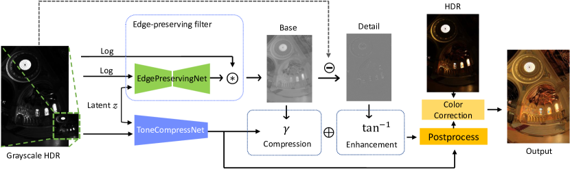
Figure 2: An overview of our tone-mapping method. Our proposed method comprises two networks: (a) an EdgePreservingNet, and (b) a ToneCompressingNet. Given an input HDR image in logarithm domain, the EdgePreservingNet generates convolutional kernels, which will be used to produce the base image. Next, we subtract the base image from the input HDR image to acquire the detail image, and then apply an enhancement operation to it. The base image is then compressed using the global tone curve predicted by the ToneCompressingNet. Eventually, the output LDR image is obtained by adding the compressed base image and enhanced detail image along with some post-processing and color correction operations.

Bilateral filtering [3] is one of the most common tone-mapping operators. The core concept behind this operator is to decompose an HDR image into a base layer and a detail layer, which respectively stands for the most part of dynamic range and the high-frequency information of the HDR image. However, the base layer and detail layer are typically decomposed by some hand-crafted edge-preserving filters and compression operations. Due to the large amount of parameters, tuning these filters and operations is usually difficult and time-consuming.

Instead of hand-crafted filters and operations, we propose a learning-based scheme as shown in Fig. 2. The proposed scheme comprises two networks: (a) an EdgePreservingNet, and (b) a ToneCompressingNet. In order to avoid artifacts, we let EdgePreservingNet be a Kernel Prediction Network (KPN) [24]. Therefore, given an input HDR image in logarithm domain, the EdgePreservingNet generates convolutional kernels to produce the base image. Next, the detail image is acquired by subtracting the base image from the input HDR image. For the purpose of better visual quality, we apply an enhancement operation to the detail image. The base image is then compressed using the global tone curve predicted by the ToneCompressingNet, which is a typical Conv-FC network. Eventually, the output LDR image is obtained by adding the compressed base image and enhanced detail image along with some post-processing and color correction operations. Fig. 3 shows an example of decomposed images.

The EdgePreservingNet and ToneCompressingNet are jointly trained using the framework of BicycleGAN, which will be described in Section III-C. It is worthwhile to mention that various random latent codes $\mathbf{z}$ are fed into these networks during training to make them able to generate various LDR images. Moreover, a latent code optimization scheme will be introduced in Section III-D to help users to find appropriate latent codes.

(a) Input HDR image	(b) Our LDR result

(c) Learned detail image	(d) Learned base image

Figure 3: Example of learned decomposed images.

III-B Tone Mapping Operators

We apply a U-Net [25] architecture to the EdgePreservingNet, which is composed of an encoder-decoder with some skip connections. As suggested in Gu et al. [12], the input HDR images are first transformed into logarithm domain and then normalized to $[0,1]$ to fit human perception. Rather than directly generating the base image, the EdgePreservingNet predicts a pixel-wise filter of size $H\times W\times K^{2}$, where $K$ is the kernel size, and $H$, $W$ is the height and width of the image. The predicted kernel at each pixel $\mathbf{w}_{p}$ is then normalized by

$$\mathbf{w}_{p}^{\prime}=\frac{\mathbf{w}_{p}}{\sum_{i=1}^{K^{2}}\mathbf{w}_{p}(i)},$$ (1)

where $i$ is termed as each element of $\mathbf{w}_{p}$. Fig. 4 shows that this normalization is critical to the tone-mapping performance.

The base image $\mathbf{I}_{\text{base}}$ is thus given by applying convolution to the input HDR image $\mathbf{I}_{\text{hdr}}$ in logarithm domain as

$${\mathbf{I}_{\text{base}}}=\sum_{p=1}^{H\times W}(\mathbf{w}_{p}^{\prime}*\log{\mathbf{I}_{\text{hdr}}})\cdot\mathds{1}_{p},$$ (2)

where $\mathds{1}_{p}$ indicates pixel $p$ having the value $1$ otherwise $0$. The detail image is then obtained by $\mathbf{I}_{\text{detail}}=\mathbf{I}_{\text{hdr}}-\mathbf{I}_{\text{base}}$.

The ToneCompressingNet consists of a series of consecutive convolution layers followed by some fully-connected layers. The network predicts the compression rate $\gamma_{\text{base}}$ as well as the degree of post-processing $\gamma_{\text{post}}$. The compressed base image is simply acquired by

$${\mathbf{I}_{\text{base}}}^{\prime}={\mathbf{I}_{\text{base}}}^{\gamma_{\text{base}}}.$$ (3)

To better preserve visual information, we define our enhancement function as

$$E(x|\alpha)=\frac{\arctan\alpha x}{\arctan\alpha},$$ (4)

where $\alpha$ is a hyper-parameter controlling the enhancement level. Specifically, $\alpha$ is set to $3.5$ in this work, so we have the enhanced detail image ${\mathbf{I}_{\text{detail}}}^{\prime}=E(\mathbf{I}_{\text{detail}}|\alpha=3.5)$. The reconstructed image is thus given by $\mathbf{I}_{\text{rec}}={\mathbf{I}_{\text{base}}}^{\prime}+{\mathbf{I}_{\text{detail}}}^{\prime}$.

To further enhance the contrast of $\mathbf{I}_{\text{rec}}$, we stretch and flatten its histogram by Eq. 4 again. However, different from detail enhancement, this operation needs to be applied on zero-mean domain. Thus, the post-processing operation is defined as

$$\mathbf{I}_{\text{post}}=E(\mathbf{I}_{\text{rec}}-\mu|\alpha=\gamma_{\text{post}})+\mu,$$ (5)

where $\mu$ is the mean illuminance of $\mathbf{I}_{\text{rec}}$.

Finally, following Tumblin et al. [26], we perform a color correction to obtain our LDR image as

$$\mathbf{I}_{\text{ldr}}=(\frac{\mathbf{I}_{\text{hdr}}^{c}}{\mathbf{I}_{\text{hdr}}})^{\beta}\cdot\mathbf{I}_{\text{post}},$$ (6)

where $\mathbf{I}_{\text{hdr}}^{c}$ denotes the color HDR image (original radiance map) and $\beta$ is set to 0.6 in this work.

III-C Training

We choose BicycleGAN as our main framework to train tone-mapping operators. Nevertheless, we replace the LSGAN loss used in BicycleGAN with a hinge loss, which has been proven to produce impressive results in [27]. The hinge loss can be expressed as

$$\begin{split}\mathcal{L}_{G}&=-\mathbb{E}_{\mathbf{x},\mathbf{y}\sim\mathbb{P}_{\text{data}},\mathbf{z}\sim\mathbb{P}_{\mathbf{z}}}[D(G(\mathbf{x},\mathbf{z}),\mathbf{y})]\\ \mathcal{L}_{D}&=-\mathbb{E}_{\mathbf{x},\mathbf{y}\sim\mathbb{P}_{\text{data}}}[min(0,-1+D(\mathbf{x},\mathbf{y}))]\\ &-\mathbb{E}_{\mathbf{x},\mathbf{y}\sim\mathbb{P}_{\text{data}},\mathbf{z}\sim\mathbb{P}_{\mathbf{z}}}[min(0,-1-D(G(\mathbf{x},\mathbf{z}),\mathbf{y}))],\end{split}$$ (7)

where $\mathcal{L}_{G}$ is the generator loss and $\mathcal{L}_{D}$ is the discriminator loss. The $\mathbf{x}$ and $\mathbf{y}$ here represent the LDR images in target domain.

To further improve the diversity, a regularization term $\mathcal{L}_{\text{div}}$ proposed by DSGAN [23] is introduced as

$$\mathcal{L}_{\text{div}}=\mathbb{E}_{\mathbf{z}_{1},\mathbf{z}_{2}\sim\mathbb{P}_{\mathbf{z}}}\left[min(\frac{\left\|G(\mathbf{x},\mathbf{z}_{1})-G(\mathbf{x},\mathbf{z}_{2})\right\|_{1}}{\left\|\mathbf{z}_{1}-\mathbf{z}_{2}\right\|_{1}},\tau)\right],\\$$ (8)

where $\tau$ determines the stability of numerical computation. Our GAN loss is hence defined as

$$\mathcal{L}_{\text{GAN}}(G,D)=\mathcal{L}_{G}+\mathcal{L}_{D}-\lambda_{\text{div}}\mathcal{L}_{\text{div}}.$$ (9)

In addition, a total variation loss $\mathcal{L}_{\text{tv}}$ is imposed on the base image to smooth the prediction as

$$\mathcal{L}_{\text{tv}}=\mathbb{E}_{\mathbf{I}_{\text{base}}\sim\mathbb{P}_{g}}\left[\sum_{p=1}^{H\times W}\left|\nabla{\mathbf{I}_{\text{base}}(p)}\right|\right],$$ (10)

where $\left|\nabla\cdot\right|$ stands for the magnitude of image gradient.

The full objective of our model is thus combined as

$$\mathcal{L}_{\text{total}}=\mathcal{L}_{\text{GAN}}(G,D)+\lambda_{\text{rec}}\mathcal{L}_{\text{rec}}+\mathcal{L}_{\text{kl}}+\mathcal{L}_{z}+\mathcal{L}_{\text{tv}},$$ (11)

where $\mathcal{L}_{rec}$, $\mathcal{L}_{kl}$, and $\mathcal{L}_{z}$ respectively represent the $L_{1}$ reconstruction loss, the KL divergence of latent codes, and the encoder loss used in the original BicycleGAN.

(a) without	(b) with

Figure 4: The effect of normalization on predicted kernels.

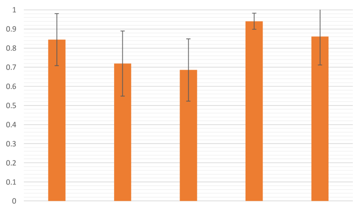
vs. Liang et al. [6]

vs. Mantiuk et al. [28]

vs. Lischinski et al. [29]

vs. Mantiuk et al. [7]

vs. Yang et al. [8]

Figure 5: User study results. Our results achieve higher probability of being selected by the subjects than the compared methods.

III-D Latent Code Optimization

Recall that tone-mapping is a subjective task, that is, people prefer different types or styles of tone-mapped images. Although our method allows users to change the style by adjusting the latent code, it is still very challenging to find appropriate ones because of the extremely huge search space. Instead of using random latent codes in testing phase, we propose a scheme that optimizes TMQI [18], which is a representative evaluation metric of tone-mapping, to help users to filter out inappropriate latent codes. Given a well-trained tone-mapping operator with fixed model parameters and an initial latent code, the latent code is then iteratively optimized by backpropagation using Adam [30] optimizer. Generally, this process converges by about 30 iterations. With this scheme, all the users need to do is select latent codes among few candidates. Note that both TMQI and our model are differentiable.

IV Experimental Results

The following experiments are conducted on Fairchild’s dataset [31]. This test set contains 105 images with diverse scenes including indoor, outdoor, daylight, and night views with a variety of image sizes. We compare our method with state-of-the-art tone-mapping methods qualitatively and quantitatively. Additionally, we provide a user study that also shows the superiority of our method over the compared methods.

IV-A Training Dataset

We collect our training dataset from multiple sources [32, 31, 33, 34, 35, 36, 37, 38, 39], which totally contains 1032 HDR images with a wide range of contents, e.g. scenes, cameras, and shooting settings. We use Luminance HDR  with the default parameters to generate LDR images, and the LDR images corresponding to each HDR image with top-3 highest TMQI scores are selected as the target images. This selection scheme makes our model has better generalization. Note that our training dataset and Fairchild’s dataset are mutually exclusive.

IV-B Implementation details

We apply random cropping and flipping augmentation to our training data. During training, the images are cropped into $256\times 256$ patches. The initial learning rates are set to $5\cdot 10^{-5}$ and $2\cdot 10^{-4}$ for the tone-mapping operator and the discriminator, respectively. The model parameters are initialized by Xavier initializer [40] and optimized by Adam optimizer with $\beta_{1}=0.9$ and $\beta_{2}=0.998$. The kernel size $K$ for EdgePreservingNet is set to $7$. The valid range of $\gamma_{\text{base}}$ and $\gamma_{\text{post}}$ are set to $[0.8,2.8]$ and $[1.7,3.7]$, respectively. The hyper-parameters $\lambda_{\text{rec}}$ and $\lambda_{\text{div}}$ are respectively set to 1 and 5. The training process takes about 1 day for 300 epochs on a single NVIDIA TITAN RTX GPU.

IV-C Qualitative Comparison

We compare our method with three representative conventional methods [7, 28, 29], one layer decomposition method [6], and two deep learning-based methods [8, 9] on Fairchild’s Dataset. The three conventional methods are implemented by Luminance HDR. For Liang et al. [6], we use their MATLAB source code with the default parameters. For Yang et al. [8], we use the pre-trained model provided by the authors. Unfortunately, the source code of Rana et al. [9] is not available, so we only compare the results reported in their paper. Fig. 7 shows that our results preserve the detail of input HDR images without halo artifacts or over enhancement. The color appearance of our results are also visually appealing. On the contrary, Lischinski et al. [29] often produce over-exposed results, and Liang et al. [6] fail to generate natural results. For deep learning-based methods, Yang et al. [8] cannot preserve the detail in highlight regions well and generate grid-like artifacts, and Rana et al. [9] show an over-saturation problem. Most importantly, these deep learning-based methods can only support one-to-one mapping, whereas our method is multimodal.

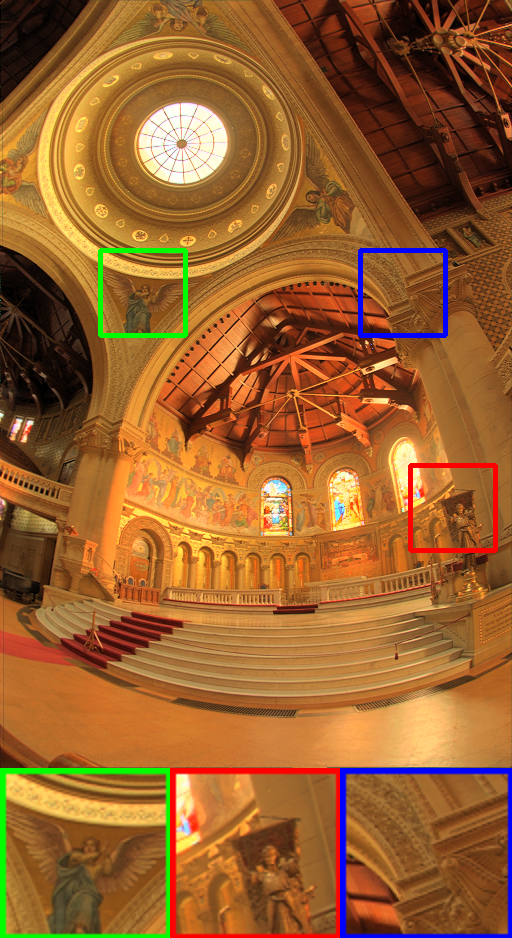
(a) Large	(b) Medium	(c) Small

Figure 6: Different detail strengths in different latent codes.

(a) linear	(b) Mantiuk et al. [28]	(c) Lischinski et al. [29]	(d) Mantiu et al. [7]

(e) Liang et al. [6]	(f) Yang et al. [8]	(g) *Rana et al. [9]	(h) Ours

(a) linear	(b) Mantiuk et al. [28]	(c) Lischinski et al. [29]	(d) Mantiuk et al. [7]

(e) Liang et al. [6]	(f) Yang et al. [8]	(g) *Rana et al. [9]	(h) Ours

Figure 7: Qualitative comparison on tone-mapping methods. Our results strike a better balance between local detail preserving and global tone compression. (* indicates the results are from their paper. The aspect ratio might be different from others.)

IV-D Diversity in different latent codes

As mentioned in Section III-A, our method is multimodal because of the framework of BicycleGAN with various random latent codes during training. Fig. 1 shows the linearity of our results with respect to latent codes. On the other hand, Fig. 6 shows that we can also control the detail strength by adjusting the latent code.

IV-E Quantitative Comparison

Besides qualitative comparisons, we also perform a quantitative comparison based on TMQI and its sub-metrics. In Table I, we list the methods of top-10 highest TMQI scores on Fairchild’s dataset. As shown in the table, our method achieves the highest TMQI and naturalness score. Although Mantiuk et al. [7] achieve the highest fidelity score among all compared methods, they often over-enhance texture detail and generate unnatural results.

TABLE I: Quantitative comparison on tone-mapping methods. The table shows that our proposed method performs competitively against existing tone-mapping methods.

Methods	TMQI	Fidelity	Naturalness
Drago et al. [41]	0.8030	0.7777	0.2289
Fattal et al. [4]	0.8126	0.8217	0.2220
Durand et al. [3]	0.8211	0.7943	0.2993
Mai et al. [42]	0.8184	0.8077	0.2554
Reinhard et al. [5]	0.8282	0.7964	0.3281
Mantiuk 08 et al. [28]	0.8447	0.8336	0.3496
Lischinski et al. [29]	0.8564	0.8381	0.4110
Mantiuk 06 et al. [7]	0.8574	0.8797	0.3412
Liang et al. [6]	0.8650	0.8074	0.5024
Yang et al. [8]	0.8465	0.7564	0.4793
Ours	0.8652	0.8064	0.5096

IV-F User Study

To further verify the performance of our method, we conduct a user study on Fairchild’s dataset [31]. Totally, 40 subjects are involved in this test. We choose the methods of top-4 highest TMQI scores on Fairchild’s dataset for comparison. The subjects are asked to select a preferable image for each pair comparison of the dataset. Then, the results are evaluated by calculating the probability of being selected by the subjects. Fig. 5 shows that our results achieve higher probability than the compared methods.

V Conclusions

We have presented a novel deep learning-based tone-mapping method. The proposed method performs favorably against existing conventional methods and learning-based methods quantitatively and qualitatively. We have also provided a user study to make the experimental results more convincing. Moreover, the proposed method can produce a variety of expert-level tone-mapped results by adjusting the latent code.

As for future work, making the latent code more explainable and easier to adjust could be a possible direction.

References

- [1] J.-Y. Zhu, R. Zhang, D. Pathak, T. Darrell, A. A. Efros, O. Wang, and E. Shechtman, “Toward multimodal image-to-image translation,” in Advances in Neural Information Processing Systems, 2017.
- [2] T. Jinno and M. Okuda, “Multiple exposure fusion for high dynamic range image acquisition,” IEEE Transactions on Image Processing, vol. 21, no. 1, pp. 358–365, Jan 2012.
- [3] F. Durand and J. Dorsey, “Fast bilateral filtering for the display of high-dynamic-range images,” ACM Trans. Graph., vol. 21, no. 3, p. 257–266, Jul. 2002. [Online]. Available: https://doi.org/10.1145/566654.566574
- [4] R. Fattal, D. Lischinski, and M. Werman, “Gradient domain high dynamic range compression,” ACM Trans. Graph., vol. 21, no. 3, p. 249–256, Jul. 2002. [Online]. Available: https://doi.org/10.1145/566654.566573
- [5] E. Reinhard, M. Stark, P. Shirley, and J. Ferwerda, “Photographic tone reproduction for digital images,” ACM Trans. Graph., vol. 21, no. 3, p. 267–276, Jul. 2002. [Online]. Available: https://doi.org/10.1145/566654.566575
- [6] Z. Liang, J. Xu, D. Zhang, Z. Cao, and L. Zhang, “A hybrid l1-l0 layer decomposition model for tone mapping,” in 2018 IEEE/CVF Conference on Computer Vision and Pattern Recognition, 2018, pp. 4758–4766.
- [7] R. Mantiuk, K. Myszkowski, and H.-P. Seidel, “A perceptual framework for contrast processing of high dynamic range images,” ACM Trans. Appl. Percept., vol. 3, no. 3, pp. 286–308, Jul. 2006. [Online]. Available: http://doi.acm.org/10.1145/1166087.1166095
- [8] X. Yang, K. Xu, Y. Song, Q. Zhang, X. Wei, and L. Rynson, “Image correction via deep reciprocating hdr transformation,” in IEEE Conference on Computer Vision and Pattern Recognition, 2018.
- [9] A. Rana, P. Singh, G. Valenzise, F. Dufaux, N. Komodakis, and A. Smolic, “Deep Tone Mapping Operator for High Dynamic Range Images,” IEEE Transactions on Image Processing, pp. 1–1, 2019. [Online]. Available: https://ieeexplore.ieee.org/document/8822603/
- [10] J. Tumblin and H. Rushmeier, “Tone reproduction for realistic images,” IEEE Comput. Graph. Appl., vol. 13, no. 6, pp. 42–48, Nov. 1993. [Online]. Available: https://doi.org/10.1109/38.252554
- [11] G. Ward, A Contrast-Based Scalefactor for Luminance Display. USA: Academic Press Professional, Inc., 1994, p. 415–421.
- [12] Bo Gu, Wujing Li, Minyun Zhu, and Minghui Wang, “Local Edge-Preserving Multiscale Decomposition for High Dynamic Range Image Tone Mapping,” IEEE Transactions on Image Processing, vol. 22, no. 1, pp. 70–79, Jan. 2013. [Online]. Available: http://ieeexplore.ieee.org/document/6272350/
- [13] G. Eilertsen, R. K. Mantiuk, and J. Unger, “A comparative review of tone-mapping algorithms for high dynamic range video,” Comput. Graph. Forum, vol. 36, no. 2, pp. 565–592, May 2017. [Online]. Available: https://doi.org/10.1111/cgf.13148
- [14] Z. Farbman, R. Fattal, D. Lischinski, and R. Szeliski, “Edge-preserving decompositions for multi-scale tone and detail manipulation,” ACM Trans. Graph., vol. 27, no. 3, p. 1–10, Aug. 2008. [Online]. Available: https://doi.org/10.1145/1360612.1360666
- [15] V. A. Patel, P. Shah, and S. Raman, “A generative adversarial network for tone mapping hdr images,” in Computer Vision, Pattern Recognition, Image Processing, and Graphics, R. Rameshan, C. Arora, and S. Dutta Roy, Eds. Singapore: Springer Singapore, 2018, pp. 220–231.
- [16] I. Goodfellow, J. Pouget-Abadie, M. Mirza, B. Xu, D. Warde-Farley, S. Ozair, A. Courville, and Y. Bengio, “Generative adversarial nets,” in Advances in Neural Information Processing Systems, 2014, pp. 2672–2680. [Online]. Available: http://papers.nips.cc/paper/5423-generative-adversarial-nets.pdf
- [17] M. Mirza and S. Osindero, “Conditional generative adversarial nets,” CoRR, vol. abs/1411.1784, 2014. [Online]. Available: http://arxiv.org/abs/1411.1784
- [18] H. Yeganeh and Z. Wang, “Objective quality assessment of tone-mapped images,” IEEE Transactions on Image Processing, vol. 22, no. 2, pp. 657–667, 2013.
- [19] J. Bao, D. Chen, F. Wen, H. Li, and G. Hua, “Cvae-gan: Fine-grained image generation through asymmetric training,” in 2017 IEEE International Conference on Computer Vision (ICCV), 2017, pp. 2764–2773.
- [20] X. Chen, Y. Duan, R. Houthooft, J. Schulman, I. Sutskever, and P. Abbeel, “Infogan: Interpretable representation learning by information maximizing generative adversarial nets,” in Advances in Neural Information Processing Systems, 2016, pp. 2172–2180.
- [21] J. Donahue, P. Krähenbühl, and T. Darrell, “Adversarial feature learning,” arXiv preprint arXiv:1605.09782, 2016.
- [22] V. Dumoulin, I. Belghazi, B. Poole, A. Lamb, M. Arjovsky, O. Mastropietro, and A. C. Courville, “Adversarially learned inference,” arXiv preprint, vol. abs/1606.00704, 2016.
- [23] D. Yang, S. Hong, Y. Jang, T. Zhao, and H. Lee, “Diversity-sensitive conditional generative adversarial networks,” in Proceedings of the International Conference on Learning Representations, 2019.
- [24] B. Mildenhall, J. T. Barron, J. Chen, D. Sharlet, R. Ng, and R. Carroll, “Burst denoising with kernel prediction networks,” in 2018 IEEE/CVF Conference on Computer Vision and Pattern Recognition, 2018, pp. 2502–2510.
- [25] O. Ronneberger, P. Fischer, and T. Brox, “U-net: Convolutional networks for biomedical image segmentation,” in Medical Image Computing and Computer-Assisted Intervention – MICCAI 2015, N. Navab, J. Hornegger, W. M. Wells, and A. F. Frangi, Eds. Cham: Springer International Publishing, 2015, pp. 234–241.
- [26] J. Tumblin and G. Turk, “Lcis: A boundary hierarchy for detail-preserving contrast reduction,” in Proceedings of the 26th Annual Conference on Computer Graphics and Interactive Techniques, ser. SIGGRAPH ’99, 1999. [Online]. Available: https://doi.org/10.1145/311535.311544
- [27] A. Brock, J. Donahue, and K. Simonyan, “Large scale GAN training for high fidelity natural image synthesis,” in 7th International Conference on Learning Representations (ICLR), 2019. [Online]. Available: https://openreview.net/forum?id=B1xsqj09Fm
- [28] R. Mantiuk, S. Daly, and L. Kerofsky, “Display adaptive tone mapping,” ACM Trans. Graph., vol. 27, no. 3, p. 1–10, Aug. 2008. [Online]. Available: https://doi.org/10.1145/1360612.1360667
- [29] D. Lischinski, Z. Farbman, M. Uyttendaele, and R. Szeliski, “Interactive local adjustment of tonal values,” ACM Trans. Graph., vol. 25, no. 3, p. 646–653, Jul. 2006. [Online]. Available: https://doi.org/10.1145/1141911.1141936
- [30] D. P. Kingma and J. Ba, “Adam: A method for stochastic optimization,” in 3rd International Conference on Learning Representations (ICLR), 2015.
- [31] “Fairchild HDR dataset,” http://rit-mcsl.org/fairchild//HDR.html.
- [32] “HDRheaven,” https://hdrihaven.com/.
- [33] “HDR-EYE,” http://mmspg.epfl.ch/hdr-eye.
- [34] H. Nemoto, P. Korshunov, P. Hanhart, and T. Ebrahimi, “Visual attention in ldr and hdr images,” 2015. [Online]. Available: http://infoscience.epfl.ch/record/203873
- [35] M.-A. Gardner, K. Sunkavalli, E. Yumer, X. Shen, E. Gambaretto, C. Gagné, and J.-F. Lalonde, “Learning to predict indoor illumination from a single image,” ACM Trans. Graph., vol. 36, no. 6, Nov. 2017. [Online]. Available: https://doi.org/10.1145/3130800.3130891
- [36] W. J. Adams, A. A. Muryy, E. W. Graf, A. J. Lugtigheid, and J. H. Elder, “The southampton york natural scenes (syns) dataset,” in Proceedings of the 12th European Conference on Visual Media Production, ser. CVMP ’15, 2015. [Online]. Available: https://doi.org/10.1145/2824840.2824857
- [37] “HDRlab,” http://www.hdrlabs.com/sibl/archive.html.
- [38] P. E. Debevec and J. Malik, “Recovering high dynamic range radiance maps from photographs,” in Proceedings of the 24th Annual Conference on Computer Graphics and Interactive Techniques, ser. SIGGRAPH ’97, 1997. [Online]. Available: https://doi.org/10.1145/258734.258884
- [39] “High Dynamic Range Specific Image Dataset (HDRSID),” http://facultymembers.sbu.ac.ir/moghaddam/index.php/main/page/10.
- [40] X. Glorot and Y. Bengio, “Understanding the difficulty of training deep feedforward neural networks,” in In Proceedings of the International Conference on Artificial Intelligence and Statistics (AISTATS’10). Society for Artificial Intelligence and Statistics, 2010.
- [41] F. Drago, K. Myszkowski, T. Annen, and N. Chiba, “Adaptive logarithmic mapping for displaying high contrast scenes,” Computer Graphics Forum, vol. 22, pp. 419–426, 2003.
- [42] Z. Mai, H. Mansour, R. Mantiuk, P. Nasiopoulos, R. Ward, and W. Heidrich, “Optimizing a tone curve for backward-compatible high dynamic range image and video compression,” IEEE Transactions on Image Processing, vol. 20, no. 6, pp. 1558–1571, June 2011.