Use of neural networks for stable, accurate and physically consistent parameterization of subgrid atmospheric processes with good performance at reduced precision

Abstract

A promising approach to improve climate-model simulations is to replace traditional subgrid parameterizations based on simplified physical models by machine learning algorithms that are data-driven. However, neural networks (NNs) often lead to instabilities and climate drift when coupled to an atmospheric model. Here we learn an NN parameterization from a high-resolution atmospheric simulation in an idealized domain by coarse graining the model equations and output. The NN parameterization has a structure that ensures physical constraints are respected, and it leads to stable simulations that replicate the climate of the high-resolution simulation with similar accuracy to a successful random-forest parameterization while needing far less memory. We find that the simulations are stable for a variety of NN architectures and horizontal resolutions, and that an NN with substantially reduced numerical precision could decrease computational costs without affecting the quality of simulations.

1 Introduction

Traditional parameterizations in general circulation models (GCMs) rely on simplified physical models and suffer from inaccuracies which lead to model biases and large uncertainties in climate projections (Bony and Dufresne, 2005, Wilcox and Donner, 2007, O’Gorman, 2012, Oueslati and Bellon, 2015, Schneider et al., 2017). One alternative to traditional parameterizations is to use machine learning (ML) algorithms to create new subgrid parameterizations (Krasnopolsky et al., 2013, Gentine et al., 2018, Rasp et al., 2018, Brenowitz and Bretherton, 2018, O’Gorman and Dwyer, 2018, Brenowitz and Bretherton, 2019, Bolton and Zanna, 2019, Yuval and O’Gorman, 2020, Han et al., 2020, Zanna and Bolton, 2020).

Two ML algorithms that have been used for climate-model parameterizations are neural networks (NNs) and random forests (RFs). O’Gorman and Dwyer (2018) trained an RF to emulate a conventional convection scheme of an atmospheric GCM and showed that when this RF parameterization is implemented in the GCM it leads to stable simulations that reproduce its climate, and the use of an RF allowed physical constraints, such as energy conservation and non-negative surface precipitation, to be respected. More recently, Yuval and O’Gorman (2020) (hereinafter referred to as YOG20) learned an RF parameterization from output of a three-dimensional high-resolution idealized atmospheric model. The parameterization led to stable simulations that replicate the climate of the high-resolution simulations at several coarse resolutions.

Despite the success of RFs in these cases, NNs have some computational advantages over RFs such as the possibility of greater accuracy and needing substantially less memory when implemented. Furthermore, an NN parameterization could potentially be implemented at reduced precision in GPUs, TPUs and even in CPUs (Vanhoucke et al., 2011) leading to very efficient parameterizations. For example, modern hardware developments that use half precision (16-bit) arithmetic on recent generation NVidia A100 GPU devices (Nvidia, 2020) allow up to 64 times the peak compute performance (0.6 PFlop/s at 16-bit precision), compared to 64-bit arithmetic (9.7 TFlop/s at 64-bit precision). Although these are theoretical peak numbers, a first exascale application in Earth science has already been realized for image classification based on GPU technology with 16-bit arithmethic (Kurth et al., 2018). Google TPUv3 devices (Jouppi et al., 2020) have similarly optimized capability (0.12 PFlop/s at 16-bit precision), for reduced precision floating point arithmetic to support deep learning applications. Furthermore, previous studies have found that using deep NNs with half-precision multipliers has little effect on accuracy when used for classification (Courbariaux et al., 2014, Miyashita et al., 2016, Micikevicius et al., 2017, Das et al., 2018). For regression tasks, which are needed for parameterizations, a reduced-precision NN might not be as accurate as a full-precision NN, but it has been argued that the dynamics at small horizontal length scales represented by parameterizations does not need the same level of precision as for large-scale dynamics because of the unpredictable and stochastic nature of the small-scale flow (Palmer, 2014). Indeed, use of reduced precision in parts of weather or climate models has already been proposed as a way to increase the speed of simulations and reduce their energy cost (Düben et al., 2014, Düben and Palmer, 2014, Düben et al., 2017).

However, there have been issues of instability and climate drift when NN parameterizations are used in GCMs. For example, Rasp et al. (2018) used NN parameterizations in the super-parametrized community atmosphere model (SPCAM) and found they are often unstable when coupled dynamically to a GCM. Rasp et al. (2018) were able to acheive a stable simulation with an NN parameterization, but they found that small changes to the configuration led to blow ups in the simulations (Rasp, 2020). Furthermore, when they quadrupled the number of embedded cloud-resolving columns (from 8 to 32) within each coarse-grid cell of SPCAM they found that instabilities returned (Brenowitz et al., 2020). Brenowitz and Bretherton (2018, 2019) learned an NN parameterization in a near-global cloud system resolving model (CRM) and were able to deal with instabilities by removing the upper-atmospheric humidity and temperature from the input space and by using a training cost function that takes into account the predictions from several forward time steps. Although these changes in the learning structure led to stable simulations at coarse resolution with the NN parameterization, the climates of these simulations drifted on longer time scales and were not accurate. Brenowitz et al. (2020) found using spectral analysis that instability occurs when GCMs are coupled to NNs that support unstable gravity waves with certain phase speeds. A study by Ott et al. (2020) tested the stability of simulations coupled to more than a hundred different NNs, and found a correlation between offline performance (i.e., the quality of predictions from NNs when they are not coupled to a GCM) and how long simulations run before they blow up. These results suggest that an exhaustive hyperparameter tuning might be necessary in order to achieve stability in GCM simulations that are coupled to NNs.

RFs might be more stable than NNs since their predictions for any given input are averages over samples in the training dataset, and thus they can automatically satisfy physical constraints such as energy conservation (O’Gorman and Dwyer, 2018, YOG20) and make conservative predictions for samples outside of the training data (NNs can also be forced to satisfy analytic constraints (Beucler et al., 2019), but such NNs have not yet been coupled to a GCM). However, the RFs and NNs in the studies mentioned above used different training datasets and preprocessed the high-resolution data differently. Therefore, it is difficult to determine if the stability arises from the different processing of the high-resolution model output or due to the the different properties of RFs compared to NNs. The two main differences in the data processing between YOG20 and the NNs studies mentioned above are that (1) the predicted tendencies were calculated accurately for the instantaneous atmospheric state (YOG20) rather than approximating them based on differences over 3-hour periods (Brenowitz and Bretherton, 2018, 2019) and that (2) the subgrid corrections were calculated independently for each physical process (YOG20) rather than for the combined effect of several processes (Rasp et al., 2018, Brenowitz and Bretherton, 2018, 2019).

Here we learn an NN parameterization using the same data processing that was used to learn an RF parameterization in YOG20. We show that implementing this parameterization in the same model at coarse resolution leads to stable simulations with a climatology that resembles the one obtained from a high-resolution simulation, and we compare the performance of an NN parameterization to the performance of an RF parameterization. We also test how the simulated climate is affected when reducing the precision of the inputs and outputs of the NN parameterization.

We first describe the high-resolution simulation from which the training data was calculated and how this data was coarse-grained (section 2). We then describe the structure of the NN parameterization and explain how this structure ensures that NN parameterization is consistent with several physical properties (section 3). We compare simulations using the NN parameterization to the high-resolution simulation and to a simulation with an RF parameterization, and we investigate the dependence of climate on the numerical precision of the NN parameterization (section 4). Finally, we give our conclusions (section 5).

2 Methods

2.1 Simulations

All simulations were run on a quasi-global aquaplanet configured as an equatorial beta-plane using the System for Atmospheric Modeling (SAM) version 6.3 (Khairoutdinov and Randall, 2003). The domain has zonal width of $6,912$km and meridional extent of $17,280$km. The distribution of sea surface temperature (SST) is specified to be the qobs SST distribution (Neale and Hoskins, 2000), which is zonally and hemispherically symmetric. There are 48 vertical levels. We use hypohydrostatic rescaling of the equations of motion with a scaling factor of 4, which increases the horizontal length scale of convection and allows us to use a horizontal grid spacing of 12km for the high-resolution simulation (referred to as hi-res) while explicitly representing both convection and planetary scale circulations in the same quasi-global simulation (Kuang et al., 2005, Pauluis and Garner, 2006, Garner et al., 2007, Boos et al., 2016, Fedorov et al., 2019). The hi-res simulation is the same simulation that was used for training in YOG20. It was recently shown that the tropical distributions of precipitation intensity and precipitation cluster size in hi-res are similar to the distributions calculated from satellite-based observations (O’Gorman et al., 2020). Further details of the model configuration are given in YOG20.

In addition to hi-res, we also consider simulations at horizontal grid spacings of 96km and 192km, which will be referred to as x8 and x16, respectively, since they correspond to coarser grid spacings by factors of 8 and 16, respectively. We ran a simulation at 96km horizontal grid spacing without an NN parameterization (x8), several simulations at 96km horizontal grid spacing with an NN parameterization (x8-NN, variants of this simulation are described in the text below), and simulations at 192km horizontal grid spacing with (x16-NN) and without (x16) an NN parameterization. All simulations were run for $600$ days. The first $100$ days are considered as spin up, and the presented results are taken from the last $500$ days of each simulation. Simulations with the NN parameterization start with initial conditions taken from the last time step of the simulations without the NN parameterization at the same resolution.

2.2 Coarse-graining and calculation of subgrid terms

The NN parameterization aims to account for unresolved processes that act in the vertical and affect thermodynamic and moisture prognostic variables. There are three thermodynamic and moisture prognostic variables in SAM (Khairoutdinov and Randall, 2003): liquid-ice static energy $h_{\rm{L}}$, total non-precipitating water mixing ratio $q_{\rm{T}}$, and precipitating water mixing ratio $q_{\rm{p}}$. Since $q_{\rm{p}}$ is a variable that varies on short time scales not typically resolved in climate models, we do not include $q_{\rm{p}}$ in the NN parameterization scheme following the “alternative” parameterization approach in YOG20. Consequently, we reformulate the equations of motion, and define a different thermodynamic variable ($H_{\rm{L}}$) that does not include the energy associated with precipitating water (text S1).

For each 3-hourly snapshot from hi-res, we coarse grain the prognostic variables ($u,v,w,H_{\rm{L}},q_{\rm{T}},q_{\rm{p}}$, where $u,v,w$ are the zonal, meridional and vertical wind, respectively), vertical advective fluxes, sedimentation fluxes, surface fluxes, tendency of non-precipitating water mixing ratio due to cloud microphysics, turbulent diffusivity, radiative heating and temperature. Coarse-graining is performed by spatial averaging as in YOG20 to horizontal grid spacings of 96km (x8) and 192km (x16).

We define the resolved flux of a given variable as the flux calculated using the dynamics and physics of SAM with the coarse-grained prognostic variables as inputs. The flux due to unresolved (subgrid) physical processes is calculated as the difference between the coarse-grained flux and the resolved flux. For example, the subgrid flux of $H_{\rm{L}}$ due to vertical advection is calculated as

$$\left({H}_{\rm{L}}\right)_{\rm{adv}}^{\rm{subg-flux}}=\left(\overline{wH_{\rm{L}}}-\overline{w}\overline{H}_{\rm{L}}\right),$$ (1)

where overbars denoted coarse-grained variables. For each high-resolution snapshot the coarse-grained prognostic fields are used to calculate the resolved vertical advective, sedimentation and surface fluxes. The subgrid fluxes are then calculated by taking the difference between the coarse-grained and resolved fluxes.

3 Neural network parameterization

3.1 Parameterization structure

The structure of the NN parameterization is broadly similar to the RF parameterization used in YOG20 except that where possible we predict fluxes and sources and sinks (rather than net tendencies in YOG20) in order to incorporate physical constraints into the NN parameterization (section 3.2). By contrast, for the RF parameterization in YOG20 it was sufficient to just predict net tendencies because the RF predicted averages over subsamples of the training dataset and thus automatically respected physical constraints such as energy conservation.

The NN parameterization is composed of two different NNs (Figure 1). The first NN, referred to as NN1, predicts the vertical profiles of the subgrid vertical advective fluxes of $H_{\rm{L}}$ ($(H_{\rm{L}})_{\rm{adv}}^{\rm{subg-flux}}$) and $q_{\rm{T}}$ ($(q_{\rm{T}})_{\rm{adv}}^{\rm{subg-flux}}$), the subgrid flux due to cloud ice sedimentation ($(q_{\rm{T}})_{\rm{sed}}^{\rm{subg-flux}}$), the coarse-grained tendency of $q_{\rm{T}}$ due to cloud microphysics ($(q_{\rm{T}})_{\rm{mic}}^{\rm{tend}}$), and the sum of the total radiative heating and the heating from phase changes of precipitation ($(H_{\rm{L}})_{\rm{rad-phase}}^{\rm{tend}}$, text S1). Thus the outputs of NN1 are

$$Y_{\rm{NN1}}=((H_{\rm{L}})_{\rm{adv}}^{\rm{subg-flux}},(q_{\rm{T}})_{\rm{adv}}^{\rm{subg-flux}},(q_{\rm{T}})_{\rm{sed}}^{\rm{subg-flux}},(q_{\rm{T}})_{\rm{mic}}^{\rm{tend}},(H_{\rm{L}})_{\rm{rad-phase}}^{\rm{tend}}),$$ (2)

where the superscript subg-flux refers to subgrid fluxes and the superscript tend refers to the total tendency due to a process. The tendencies due to cloud microphysics, radiative heating and heating from phase changes of precipitation are treated as entirely subgrid. In the case of cloud microphysics and phase changes of precipitation, this is because it is not possible to calculate the resolved values of these processes when $q_{\rm{p}}$ is not used as a prognostic variable in the simulations (text S1). Tendencies are predicted at the lowest 30 “full” model levels (below $z=13.9$km), while subgrid ice sedimentation fluxes are predicted at the lowest 30 “half” model levels, and vertical advective fluxes are predicted at the 29 “half” model levels above the surface (since advective fluxes is zero at the surface over ocean). Thus, NN1 has $29\times 2+30\times 3=148$ outputs. We do not use NN1 to predict outputs for levels above $13.9$km ($\approx 134$hPa) since the NN parameterization is not accurate at these levels, we want to avoid predicting near the sponge layer which is active at heights above $20$km, and the predicted tendencies and subgrid fluxes are small above $13.9$km with the exception of radiative heating. Above 13.9km the subgrid fluxes and microphysical tendency are set to zero and the radiative heating tendencies calculated at coarse resolution from SAM are used.

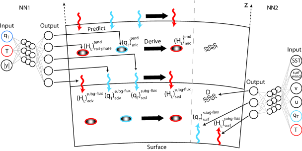
Figure 1: Illustration of the parameterization structure. There are two different NNs included in the parameterization, each having its own inputs and outputs (full description in section 3.1). Arrows indicate subgrid fluxes due to vertical advection and sedimentation, and ellipses indicate tendencies associated with sources/sinks due to cloud microphysics, radiation and phase changes of precipitating water. Blue (red) color indicates a variable, tendency or flux associated with moisture (energy).

The inputs for NN1 are the resolved vertical profiles of $q_{\rm{T}}$ and temperature ($T$), as well as the distance to the equator ($|y|$, which is a proxy for insolation and surface albedo), giving $30\times 2+1=61$ inputs. We verified that using top of atmosphere insolation as input instead of the distance to equator does not change the results presented in this study (Figure S1). We found that using all $48$ levels of $T$ and $q_{\rm{T}}$ as inputs in NN1 leads to an instability, possibly related to instabilities found previous studies when $q_{\rm{p}}$ is not used a prognostic variable (Brenowitz and Bretherton, 2019, Brenowitz et al., 2020, YOG20). However, here we include inputs up to the lower stratosphere while Brenowitz and Bretherton (2019) and Brenowitz et al. (2020) removed some inputs above the mid-troposphere to achieve stability, whereas here it is sufficient to not use inputs in the stratosphere.

The second NN, referred to as NN2, predicts subgrid surface fluxes of $H_{\rm{L}}$ and $q_{\rm{T}}$ and the coarse-grained vertical turbulent diffusivity ($\overline{D}$) that is used for $H_{\rm{L}}$ and $q_{\rm{T}}$. We only predict $\overline{D}$ in the lower troposphere (the 15 model levels below $5.7$km) because it decreases in magnitude with height (YOG20), and the diffusivity calculated at coarse resolution from SAM is used above $5.7$km. Hence the outputs of NN2 are

$$Y_{\rm{NN2}}=(\overline{D},(h_{\rm{L}})_{\rm{surf}}^{\rm{subg-flux}},(q_{\rm{T}})_{\rm{surf}}^{\rm{subg-flux}}),$$ (3)

giving $15+1+1=17$ outputs. The inputs of NN2 are chosen to be the lower tropospheric vertical profiles of $T$, $q_{\rm{T}}$, $u$, $v$, surface wind speed (wind_surf) and SST, so that $X_{\rm{NN2}}=(T,q_{\rm{T}},u,v,\rm{wind_{\rm{surf}}},SST)$, giving $4\times 15+1+1=62$ features, where $v$ in the southern hemisphere is multiplied by $-1$ when used as an input (see further discussion in YOG20).

The tendencies due to subgrid vertical advective, sedimentation and surface fluxes are calculated online (i.e., when running SAM with the parameterization) from the predicted fluxes. The subgrid energy flux due to ice sedimentation is also calculated online as

$$(H_{\rm{L}})_{\rm{sed}}^{\rm{subg-flux}}=-L_{\rm{s}}(q_{\rm{T}})_{\rm{sed}}^{\rm{subg-flux}},$$ (4)

where $L_{\rm{s}}$ is the latent heat of sublimation. Similarly, the tendency of energy due to cloud microphysics is calculated online as

$$(H_{\rm{L}})_{\rm{mic}}^{\rm{tend}}=-L_{\rm{p}}(q_{\rm{T}})_{\rm{mic}}^{\rm{tend}},$$ (5)

where $L_{\rm{p}}=L_{\rm{c}}+L_{\rm{f}}(1-\omega_{\rm{p}})$ is the effective latent heat associated with precipitation ($L_{\rm{c}}$ and $L_{\rm{f}}$ are the latent heat of condensation and fusion, respectively, and $\omega_{\rm{p}}$ is the precipitation partition function determining the ratio between ice and liquid phases).

The results presented in the main paper are for NNs (both NN1 and NN2) with five layers (four hidden layers) with 128 nodes and rectified linear unit (ReLu) activation functions. Results for different NN architectures are shown in the supplementary information (Figure S2). More details about the train and test datasets, the NNs training protocol and how inputs and outputs are rescaled can be found in the supplementary information (text S2)

When running simulations with the NN parameterization, we limit the predictions of $q_{\rm{T}}$ fluxes and tendencies such that we prevent $q_{\rm{T}}$ from being assigned with negative values. More specifically, if the NN parameterization predicts any flux or any tendency at any vertical level that would lead to negative $q_{\rm{T}}$ values if it acted on its own, we reduce this tendency or flux magnitude such that the minimal value that can be assigned to $q_{\rm{T}}$ is zero. Removing this constraint (and allowing $q_{\rm{T}}$ to be assigned with negative values) leads to a substantially different climate when the NN parameterization is used, although the simulations remain stable.

3.2 Physical consistency of the parameterization

Previous studies that used NN parameterizations usually predicted the sum of tendencies due to several different processes as a single output (Gentine et al., 2018, Rasp et al., 2018, Brenowitz and Bretherton, 2018, 2019). The coarse-graining and calculation of subgrid terms that is used in this study (section 2.2) enables us to predict the effect of each process on the prognostic variables separately (section 3.1), and where possible, the effect is diagnosed from other predicted outputs (equations 4 and 5). Furthermore, the NN parameterization predicts fluxes instead of tendencies where possible. These differences make the NN parameterization presented in this study physically consistent in the following ways:

1. Predicting the subgrid fluxes due to vertical advection instead of the subgrid tendencies guarantees energy and water are conserved by these fluxes. Similarly, predicting the flux due to sedimentation guarantees that changes in the energy of the atmospheric column due to sedimentation are only due to sedimentation that reaches the surface.

2. Changes in $H_{\rm{L}}$ due to cloud microphysics and ice sedimentation are not predicted by the NN, but are instead diagnosed from equations 4 and 5 (Figure 1). Diagnosing these tendencies guarantees that the sources or sinks of energy at each grid point due to cloud microphysics and sedimentation are consistent with the amount of moisture that was subtracted or added at that grid point.

3. The NN predicts the coarse-grained vertical diffusivity (instead of predicting subgrid diffusive tendencies or fluxes) which ensures that diffusive fluxes are downgradient and conserve energy and water in each atmospheric column.

4. The precipitation is diagnosed from the NN outputs (text S1). Diagnosing the precipitation was not done in some previous studies that used NN parameterization in which the NN was used to predict precipitation directly (Rasp et al., 2018) or the NN outputs could only be used to predict the difference between precipitation minus evaporation (Brenowitz and Bretherton, 2019).

Properties a,b, and c ensure that the NN parameterization exactly conserves energy in the sense that the column integrated frozen moist static energy is conserved in the absence of radiative heating, heating from phase changes of precipitation, surface fluxes, and conversion of condensate to graupel or snow (see Text S3).

4 Results

4.1 Simulation with neural-network parameterization

To assess the NN parameterization, we compare the climates of x8, x8-NN (using NNs with five fully connected layers, text S2) and the hi-res. We focus on the zonal- and time-mean precipitation distribution (Figure 2a) and the frequency distribution of the 3-hourly precipitation rate (Figure 2b). The frequency distribution is known to be sensitive to subgrid parameterization of moist convection (Wilcox and Donner, 2007), and the latitudinal distribution of mean precipitation is especially sensitive to subgrid parameterizations in the zonally and hemispherically symmetric aquaplanet configuration used here (Möbis and Stevens, 2012). The frequency distribution is estimated using $34$ bins that are equally spaced in the logarithm of precipitation rate, where the lowest bin starts at $1\rm{mm\leavevmode\nobreak\ day^{-1}}$, and the distribution is normalized such that it integrates to one when considering the whole distribution (including values lower than $1\rm{mm\leavevmode\nobreak\ day^{-1}}$). The hi-res and the x8-NN simulations exhibits a similar double ITCZ structure, both in amplitude and in the latitudinal structure (Figure 2a). Note that the presence of a double ITCZ in hi-res is likely to be dependent on the exact domain and SST distribution. In contrast, the x8 simulation exhibits a single ITCZ (Figure 2a), highlighting the sensitivity of the tropical circulation to changes in the horizontal resolution and to the inclusion of the NN parameterization. Also the frequency distributions of precipitation in the x8-NN closely matches that of hi-res ($R^{2}=0.99$ as measured across bins), although x8-NN overestimates the extreme events, while the frequency distribution in x8 differ substantially from the distribution of hi-res ($R^{2}=0.35$) especially for weak and extreme precipitation events (Figure 2b). The NN parameterization also brings the zonal- and time-means of the zonal wind, meridional wind, eddy kinetic and non-precipitating water closer to the hi-res climatology, and outperforms the x8 simulation for these variables (table S1). We find that these results are reproduced when the NN1 architecture is changed to have only three or four layers (Figure S2, although the amplitude of the equatorial minimum of precipitation slightly varies between simulations). All the simulations we ran were stable and without climate drift, and even a substantially less accurate NN parameterization with two layers for NN1 (table S2) leads to stable simulations, though it does not capture the precipitation distributions (Figure S2). When training an NN parameterizations for a coarse-graining factor of x16 and coupling it to a simulation with the corresponding grid spacing, similar results are obtained and precipitation distributions are captured correctly (Figure S3). Overall, we find that coupling an NN parameterization to a simulation at coarse-resolution leads to a climate that is similar to the hi-res climate, and that the stability of simulations is not sensitive to the NN architecture, hyperparameter tuning or the horizontal resolution of the simulations.

Several approximations where made when deriving the instantaneous precipitation rate (text S1). These approximations and inaccuracies in the NN predictions result in negative 3-hourly surface precipitation in $20\%$ of samples in the x8-NN simulation. Nevertheless, almost all of the negative values are very small, and only $0.03\%$ of samples are less than $-1\rm{mm\leavevmode\nobreak\ day^{-1}}$.

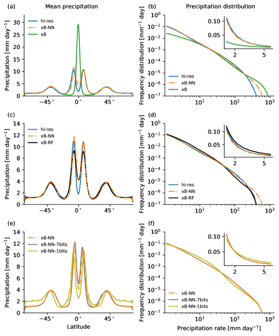
Figure 2: (a,c,e) Zonal- and time-mean precipitation rate as a function of latitude and (b,d,f) frequency distribution of 3-hourly precipitation rate. Results are shown for the high-resolution simulation (hi-res in blue; panels a-d), the coarse-resolution simulation (x8 in green; panels a-b), the coarse-resolution simulation with the NN parameterization (x8-NN in orange dash-dotted; panels a-f), the coarse-resolution simulation with the RF parameterization (x8-RF in black; panels c-d), and simulations with reduced numerical precision of the inputs and outputs of the NN parameterization with 7 significant bits in the mantissa (x8-NN-7bits in gray; panels e-f), and 1 significant bit in the mantissa (x8-NN-1bits in yellow; panels e-f) as compared to 23 bits in the mantissa for x8-NN. The frequency distribution is shown for axes with linear scale in the insets of b,d,f.

4.2 Comparing neural network and random forest parameterizations

In this section we compare the offline and online performance of NN parameterization to the (“alternative”) RF parameterization that was developed in YOG20 and also did not include $q_{\rm{p}}$. For offline performance (performance when not coupled to a GCM), we find that the NN parameterization outperforms the RF parameterization across all variables (Figure S4, text S4). Yet, the online performance of the x8-NN and x8-RF simulations is comparable (Figure 2c,d and table S1). Both x8-NN and x8-RF have a double ITCZ as in hi-res. The x8-NN simulation better captures the frequency distribution at most precipitation rates, though for extreme events x8-RF is more accurate (Figure 2d). Other climatological measures such as mean $q_{\rm{T}}$, meridional and zonal wind and eddy kinetic energy are better captured by x8-RF (table S1).

One advantage of NN is that it requires less memory compared to RF. For example, for x8, NN1 is 0.3 MB and NN2 is 0.2 MB when stored in netcdf format at single precision, which is $\approx 1900$ times less memory compared to the memory needed to store the RF parameterization. Another advantage of the NN parameterization is that the x8-NN simulation requires less CPU time than the x8-RF simulation by a factor of $1.25$, although both require much less CPU time than hi-res (by a factor of $54$ in the case of x8-NN).

4.3 Reduced-precision parameterization

As discussed in the introduction, NN parameterizations run at reduced precision could bring considerable savings in speed and energy. To test the effect of reduced precision NNs, we run simulations in which the scaled inputs and outputs of the NNs are reduced in precision. Such simulations aim to check how precise the outputs and inputs have to be to give a similar climate to the full precision. In our default configuration, SAM and the NNs are evaluated in single precision which corresponds to 23 bits in the mantissa. We reduce the precision by rounding to 7,5, 3 and 1 bits in the mantissa and the resulting simulations are referred to as x8-NN-7bits, x8-NN-5bits, x8-NN-3bits and x8-NN-1bits, while keeping the same number of bits in the exponent (8 bits). Note that the 7 bits in the mantissa corresponds to the bfloat16 “brain” floating-point (7 bits in the mantissa, 8 in the exponent and 1 to determine the sign) which is used in TPUs.

For x8-NN-7bits and x8-NN-5bits simulations we find that the resulting climate is similar, while reducing the precision to x8-NN-3bits leads to a small degradation and keeping only 1 bit in the mantissa clearly degrades the results (table S1, Figure 2e,f). Overall, we find that it is possible to reduce the precision of inputs and outputs even beyond bfloat16 format without substantially affecting the climate of the simulations, suggesting that NN parameterizations at reduced precision could bring substantial advantages in speed and power requirements.

5 Conclusions

In this study we show that an NN parameterization with a physically motivated structure learned from coarse-grained output of a three-dimensional high-resolution simulation of the atmosphere can be dynamically coupled to the atmospheric model at coarse resolution to give stable simulations with a climate that is close to that of the high-resolution simulation. In contrast to the approach in Rasp et al. (2018) we find that simulations with NN parameterization are stable for a variety of configurations, and in contrast to Brenowitz and Bretherton (2018, 2019) they do not exhibit climate drift. Furthermore, in contrast to Ott et al. (2020) we find that achieving stable simulations does not require the NN parameterization to be very accurate in an offline test, and a mediocre performing NN1 with two layers (i.e., one hidden layer) is stable when coupled to SAM.

We use the same high-resolution model output for training that was used by YOG20, which suggests that the stability of simulations with an RF parameterization in previous studies (O’Gorman and Dwyer, 2018, YOG20) is not only possible with RFs since we find NNs to be robustly stable as well. Instead, the stability of simulations with NN parameterizations may require accurate processing of the high-resolution model output to obtain subgrid tendencies and fluxes. (in addition to not including stratospheric levels). The main differences in the processing used here compared to previous studies with NN parameterizations of atmospheric subgrid processes are that the contribution of subgrid terms were calculated using the equations of the model for the instantaneous state of the atmosphere rather than approximating them based on differences over 3-hour periods (Brenowitz and Bretherton, 2018, 2019) and that subgrid corrections were calculated independently for each physical process. The latter allows us to encapsulate more physics in the parameterization, such as by calculating fluxes and sinks rather than net tendencies. A direct comparison between an RF and NN parameterizations shows that although NNs are more accurate in offline tests, when coupling the parameterizations to the atmospheric model at coarse resolution, both parameterizations have comparable results. Overall, our results imply that careful and accurate processing of the high-resolution output that is used for the training may be more important than intensive hyperparameter tuning of an ML algorithm. The time step in our coarse-resolution simulations cannot be larger than roughly 75 seconds because of the explicit time stepping of turbulent diffusion in SAM , and future work is needed to extend these results to longer time steps and to simulations with land and topography.

Finally we show that reducing the numerical precision of the inputs and outputs of the NN parameterization to bfloat16 floating-point format leads to a similar climate compared to using single precision. This implies that NN parameterizations with reduced precision could be used for faster training, and more importantly, for reducing the computational resources and energy needed to run climate simulations. To further investigate the feasibility of NN parameterizations with reduced precision, future work should also test NN parameterizations that were trained with reduced precision, such that the weights, biases and multiplications used during forward propagation of the NN are performed at reduced precision. Our results also suggest that the simulated climate may not be strongly affected by reducing the precision of conventional parameterizations or super parameterizations, but in those cases it would likely be necessary to check for each particular parameterization which parts of the algorithm can be safely reduced in precision (Düben et al., 2017).

Acknowledgments

We thank Bill Boos for providing the output from the high-resolution simulation, and Tamar Regev for help in creating figure 1 in this manuscript. We acknowledge high-performance computing support from Cheyenne (doi:10.5065/D6RX99HX) provided by NCAR’s Computational and Information Systems Laboratory, sponsored by the National Science Foundation. We acknowledge support from the EAPS Houghton-Lorenz postdoctoral fellowship and NSF AGS-1552195.

Code availability

Associated code, processed data from simulations with neural network and random forest parameterizations, trained neural network parameterizations and (a link to) the output of the high-resolution simulation are available at zenodo.org (doi:10.5281/zenodo.4118346).

References

- Beucler et al. (2019) T. Beucler, S. Rasp, M. Pritchard, and P. Gentine. Achieving conservation of energy in neural network emulators for climate modeling. preprint at https://arxiv.org/abs/1906.06622, 2019.
- Bolton and Zanna (2019) T. Bolton and L. Zanna. Applications of deep learning to ocean data inference and subgrid parameterization. Journal of Advances in Modeling Earth Systems, 11(1):376–399, 2019.
- Bony and Dufresne (2005) S. Bony and J.-L. Dufresne. Marine boundary layer clouds at the heart of tropical cloud feedback uncertainties in climate models. Geophysical Research Letters, 32(20):L20806, 2005.
- Boos et al. (2016) W. R. Boos, A. Fedorov, and L. Muir. Convective self-aggregation and tropical cyclogenesis under the hypohydrostatic rescaling. Journal of the Atmospheric Sciences, 73(2):525–544, 2016.
- Brenowitz and Bretherton (2018) N. D. Brenowitz and C. S. Bretherton. Prognostic validation of a neural network unified physics parameterization. Geophysical Research Letters, 45(12):6289–6298, 2018.
- Brenowitz and Bretherton (2019) N. D. Brenowitz and C. S. Bretherton. Spatially extended tests of a neural network parametrization trained by coarse-graining. Journal of Advances in Modeling Earth Systems, 11:2727–2744, 2019.
- Brenowitz et al. (2020) N. D. Brenowitz, T. Beucler, M. Pritchard, and C. S. Bretherton. Interpreting and stabilizing machine-learning parametrizations of convection. arXiv preprint arXiv:2003.06549, 2020.
- Courbariaux et al. (2014) M. Courbariaux, Y. Bengio, and J.-P. David. Training deep neural networks with low precision multiplications. arXiv preprint arXiv:1412.7024, 2014.
- Das et al. (2018) D. Das, N. Mellempudi, D. Mudigere, D. Kalamkar, S. Avancha, K. Banerjee, S. Sridharan, K. Vaidyanathan, B. Kaul, E. Georganas, et al. Mixed precision training of convolutional neural networks using integer operations. arXiv preprint arXiv:1802.00930, 2018.
- Düben and Palmer (2014) P. D. Düben and T. Palmer. Benchmark tests for numerical weather forecasts on inexact hardware. Monthly Weather Review, 142(10):3809–3829, 2014.
- Düben et al. (2014) P. D. Düben, H. McNamara, and T. N. Palmer. The use of imprecise processing to improve accuracy in weather & climate prediction. Journal of Computational Physics, 271:2–18, 2014.
- Düben et al. (2017) P. D. Düben, A. Subramanian, A. Dawson, and T. Palmer. A study of reduced numerical precision to make superparameterization more competitive using a hardware emulator in the OpenIFS model. Journal of Advances in Modeling Earth Systems, 9(1):566–584, 2017.
- Fedorov et al. (2019) A. V. Fedorov, L. Muir, W. R. Boos, and J. Studholme. Tropical cyclogenesis in warm climates simulated by a cloud-system resolving model. Climate Dynamics, 52(1-2):107–127, 2019.
- Garner et al. (2007) S. T. Garner, D. M. W. Frierson, I. M. Held, O. Pauluis, and G. K. Vallis. Resolving convection in a global hypohydrostatic model. Journal of the Atmospheric Sciences, 64(6):2061–2075, 2007.
- Gentine et al. (2018) P. Gentine, M. Pritchard, S. Rasp, G. Reinaudi, and G. Yacalis. Could machine learning break the convection parameterization deadlock? Geophysical Research Letters, 45(11):5742–5751, 2018.
- Han et al. (2020) Y. Han, G. J. Zhang, X. Huang, and Y. Wang. A moist physics parameterization based on deep learning. Journal of Advances in Modeling Earth Systems, page e2020MS002076, 2020.
- Jouppi et al. (2020) N. P. Jouppi, D. H. Yoon, G. Kurian, S. Li, N. Patil, J. Laudon, C. Young, and D. Patterson. A domain-specific supercomputer for training deep neural networks. Communications of the ACM, 63(7):67–78, 2020.
- Khairoutdinov and Randall (2003) M. F. Khairoutdinov and D. A. Randall. Cloud resolving modeling of the ARM summer 1997 IOP: Model formulation, results, uncertainties, and sensitivities. Journal of the Atmospheric Sciences, 60(4):607–625, 2003.
- Krasnopolsky et al. (2013) V. M. Krasnopolsky, M. S. Fox-Rabinovitz, and A. A. Belochitski. Using ensemble of neural networks to learn stochastic convection parameterizations for climate and numerical weather prediction models from data simulated by a cloud resolving model. Advances in Artificial Neural Systems, 2013:1–13, 2013.
- Kuang et al. (2005) Z. Kuang, P. N. Blossey, and C. S. Bretherton. A new approach for 3D cloud-resolving simulations of large-scale atmospheric circulation. Geophysical Research Letters, 32(2), 2005. doi: 10.1029/2004GL021024. URL https://doi.org/10.1029/2004GL021024.
- Kurth et al. (2018) T. Kurth, S. Treichler, J. Romero, M. Mudigonda, N. Luehr, E. Phillips, A. Mahesh, M. Matheson, J. Deslippe, M. Fatica, et al. Exascale deep learning for climate analytics. In SC18: International Conference for High Performance Computing, Networking, Storage and Analysis, pages 649–660. IEEE, 2018.
- Micikevicius et al. (2017) P. Micikevicius, S. Narang, J. Alben, G. Diamos, E. Elsen, D. Garcia, B. Ginsburg, M. Houston, O. Kuchaiev, G. Venkatesh, et al. Mixed precision training. arXiv preprint arXiv:1710.03740, 2017.
- Miyashita et al. (2016) D. Miyashita, E. H. Lee, and B. Murmann. Convolutional neural networks using logarithmic data representation. arXiv preprint arXiv:1603.01025, 2016.
- Möbis and Stevens (2012) B. Möbis and B. Stevens. Factors controlling the position of the Intertropical Convergence Zone on an aquaplanet. Journal of Advances in Modeling Earth Systems, 4:M00A04, 2012.
- Neale and Hoskins (2000) R. B. Neale and B. J. Hoskins. A standard test for AGCMs including their physical parametrizations: I: The proposal. Atmospheric Science Letters, 1:101–107, 2000.
- Nvidia (2020) Nvidia. Nvidia A100 tensor core GPU architecture. Technical report, 2020. URL https://www.nvidia.com/content/dam/en-zz/Solutions/Data-Center/nvidia-ampere-architecture-whitepaper.pdf.
- O’Gorman (2012) P. A. O’Gorman. Sensitivity of tropical precipitation extremes to climate change. Nature Geoscience, 5(10):697–700, 2012.
- O’Gorman and Dwyer (2018) P. A. O’Gorman and J. G. Dwyer. Using machine learning to parameterize moist convection: Potential for modeling of climate, climate change, and extreme events. Journal of Advances in Modeling Earth Systems, 10(10):2548–2563, 2018.
- O’Gorman et al. (2020) P. A. O’Gorman, Z. Li, W. R. Boos, and J. Yuval. Response of extreme precipitation to climate warming in quasi-global aquaplanet simulations at high resolution. submitted to Philosophical Transactions of the Royal Society A, 2020.
- Ott et al. (2020) J. Ott, M. Pritchard, N. Best, E. Linstead, M. Curcic, and P. Baldi. A Fortran-Keras deep learning bridge for scientific computing. arXiv preprint arXiv:2004.10652, 2020.
- Oueslati and Bellon (2015) B. Oueslati and G. Bellon. The double ITCZ bias in CMIP5 models: interaction between SST, large-scale circulation and precipitation. Climate Dynamics, 44(3-4):585–607, 2015.
- Palmer (2014) T. N. Palmer. More reliable forecasts with less precise computations: a fast-track route to cloud-resolved weather and climate simulators? Philosophical Transactions of the Royal Society A: Mathematical, Physical and Engineering Sciences, 372(2018):20130391, 2014.
- Pauluis and Garner (2006) O. Pauluis and S. Garner. Sensitivity of radiative–convective equilibrium simulations to horizontal resolution. Journal of the atmospheric sciences, 63(7):1910–1923, 2006.
- Rasp (2020) S. Rasp. Coupled online learning as a way to tackle instabilities and biases in neural network parameterizations: general algorithms and Lorenz96 case study (v1.0). Geoscientific Model Development, pages 2185––2196, 2020.
- Rasp et al. (2018) S. Rasp, M. S. Pritchard, and P. Gentine. Deep learning to represent subgrid processes in climate models. Proceedings of the National Academy of Sciences of the United States of America, 115:9684–9689, 2018.
- Schneider et al. (2017) T. Schneider, J. Teixeira, C. S. Bretherton, F. Brient, G. Pressel, K, C. Schär, and A. P. Siebesma. Climate goals and computing the future of clouds. Nat. Clim. Change, 7:3–5, 2017.
- Vanhoucke et al. (2011) V. Vanhoucke, A. Senior, and M. Z. Mao. Improving the speed of neural networks on CPUs. In Proc. Deep Learning and Unsupervised Feature Learning, Neural Information Processing Systems Workshop, 2011.
- Wilcox and Donner (2007) E. M. Wilcox and L. J. Donner. The frequency of extreme rain events in satellite rain-rate estimates and an atmospheric general circulation model. Journal of Climate, 20(1):53–69, 2007.
- Yuval and O’Gorman (2020) J. Yuval and P. A. O’Gorman. Stable machine-learning parameterization of subgrid processes for climate modeling at a range of resolutions. Nature Communications, 11(1):1–10, 2020.
- Zanna and Bolton (2020) L. Zanna and T. Bolton. Data-driven equation discovery of ocean mesoscale closures. Geophysical Research Letters, page e2020GL088376, 2020.