Generally Applicable Formalism for Modeling the Observable Signatures of Inflows, Outflows, and Moving Coronal Plasma Close to Kerr Black Holes

Abstract

We present a generally applicable formalism for modeling the emission, absorption, reflection, and reprocessing of radiation by moving plasma streams close to a Kerr Black hole. The formalism can be used to investigate the observational signatures of a wide range of phenomena, including: (i) the reflection of coronal X-ray radiation off plasma plunging from the inner edge of a black hole accretion disk towards the black hole; (ii) the reflection of coronal X-ray emission off the upper layers of a geometrically thick accretion flow; (iii) the illumination of the accretion disk by a corona moving with relativistic velocities towards or away from the accretion disk; (iv) the emission from a jet forming close to the black hole. After introducing the general relativistic treatment, we show the results for a fast wind forming close to a Kerr black hole. The approach presented here can be used to model X-ray spectral, timing, reverberation, and polarization data.

1 Introduction

In this paper, we show how to model the emission, absorption, and reprocessing of radiation by inflows, outflows, or moving coronal plasma close to Kerr black holes. The formalism is well suited to be used in general relativistic ray tracing codes (e.g. Li et al., 2005; Schnittman & Krolik, 2009, 2010; Krawczynski, 2012; Dauser et al., 2013; Wilkins & Gallo, 2015; Beheshtipour et al., 2017; Choudhury et al., 2017; Tamborra et al., 2018; Zhang et al., 2019). Such codes are likely to continue to play an important role for the analysis and interpretation of the data from current and upcoming X-ray missions. General Relativistic (Radiation) MagnetoHydroDynamic (GR(R)MHD) simulations have made enormous progress over the last decade (see e.g. Kinch et al., 2019; Porth et al., 2019; Liska et al., 2020, and references therein). However, the predicted X-ray energy spectra will depend on a number of parameters describing the background spacetime (i.e. the black hole mass and spin), the properties of the accreted plasma (e.g. the accretion rate, the structure of the accreted magnetic field, and the elemental composition of the accreted plasma) that impact the accretion flow dynamics and thus the emitted energy spectra. It seems unlikely that a sufficiently large number of GR(R)MHD simulations can be run (each individual simulation taking substantial time on a supercomputer) to enable the direct comparison of the simulated GR(R)MHD results with the X-ray data of many different astrophysical sources. More likely, the GR(R)MHD results need to be used to inform simpler treatments, such as the raytracing codes mentioned above. The latter can then be used in turn to simulate a sufficiently large number of configurations to allow for a quantitative comparison of the simulated and observed data. The work described in this paper can be used to add emitting, absorbing, reflecting or Comptonizing inflows, outflows, or relativistically moving coronal plasma to such raytracing codes.

Several authors studied the impact of a moving corona on the illumination of the accretion disk and the shape of the reflected Fe K$\alpha$ line emission (Reynolds & Fabian, 1997; Beloborodov, 1999; Fukumura & Kazanas, 2007; Wilkins & Fabian, 2012; Dauser et al., 2013). These studies either considered flat spacetime geometries (Reynolds & Fabian, 1997; Beloborodov, 1999), or were limited to the motion of the emitting gas along the spin axis of the black hole (Fukumura & Kazanas, 2007; Wilkins & Fabian, 2012; Dauser et al., 2013). For notable exceptions see (Hartnoll & Blackman, 2002; Dovčiak et al., 2004). In contrast, the approach presented in this paper can be used to parameterize gas moving along any streamline or surface. Application of the results of this paper include the phenomenological modeling of inflows and outflows. A number of physics motivated wind and jet models have been put forward in the literature. Most of the models however, are limited to describing the plasma motion far away from the black hole where the spacetime is approximately flat and a Newtonian approach is warranted (e.g. Blandford, 1976; Blandford & Payne, 1982; Blandford & Begelman, 1999; Fukumura et al., 2010; Higginbottom et al., 2014; Yuan & Narayan, 2014; Miller et al., 2015; Waters et al., 2016; Nomura & Ohsuga, 2017; Blandford et al., 2019; Abdikamalov et al., 2020, and references therein). In contrast, the formalism discussed here can be used all the way to the event horizon.

The rest of the paper is structured as follows. We describe the formalism in Section 2. As an example, we model the emission reflecting off an accretion disk and a fast wind being launched close to a black hole in Section 3. We conclude with a discussion of other applications of the formalism in Section 4.

2 General Relativistic Description of Plasma Moving Towards or Away from Kerr Black Holes

2.1 Flow Geometry and Kinematics

We use the Kerr metric in Boyer Lindquist coordinates $x^{\mu}\,=\,(t,r,\theta,\phi)$. We employ geometric units, and set $M\,=\,1$. The spin parameter $a$ can take values between -1 (maximally counter-rotating) and 1 (maximally rotating). We assume that the flow can be parameterized by the functions $r(P)$ and $\theta(P)$ of $N$ parameters $P=\left\{p1,p2,...,p_{N}\right\}$ with the parameter $p_{1}$ increasing monotonically along the plasma streamlines. In the simplest case, the flow can be approximated to have the geometry of an axially symmetric surface, e.g., a dense wind, or the photosphere of a geometrically thick accretion flow. In that case, the parameter $p_{1}$ suffices to define the surface.

As an example, we will consider a conical outflow launched at $r=r_{\rm l}$ into the upper hemisphere with half opening angle $\alpha$. In cylindrical coordinates ($\rho$,$z$), the outflow can be described by the equation:

$$z(\rho)\,=\,(\rho-r_{\rm l})/\tan{\alpha}$$ (1)

for $\rho\geq r_{\rm l}$. The corresponding Boyer Lindquist coordinates are:

$$r(P) = \,\sqrt{\rho^{2}+z(\rho)^{2}}$$ (2)

$$\theta(P) = \arctan{(z(\rho)/\rho)}.$$ (3)

The two functions $r(P)$ and $\theta(P)$ with $P=\left\{p_{1}\right\}$, $p_{1}=\rho$ fully determine the geometry of the flow. One could model a 3-D flow by adding another parameter, e.g. $p_{2}\,=\,r_{\rm l}$, so that $p_{2}$ marks adjacent surfaces.

We will now derive an expression for the four velocity of the flow v given two additional functions: (i) the velocity of the flow $\beta(P)$ relative to a local Zero Angular Momentum Observer (ZAMO) in units of the speed of light, and (ii) the angular velocity of the flow $\Omega(P)$. The parameterization of $\beta(P)$ and $\Omega(P)$ can be chosen freely, i.e. one can use the results from a GR(R)MHD simulation or other physically motivated prescriptions, or use a phenomenological parametrization with fitting parameters that need to be inferred from confronting the model predictions with experimental data.

For our example, we assume that the flow co-rotates with the accretion plasma at ($r=r_{\rm l}$, $\theta=\pi/2$) and accelerates such that the Lorentz factor $\gamma\,=\,(1-\beta^{2})^{-1/2}$ relative to the ZAMO is given by:

$$\gamma(P)=\gamma_{\rm l}+\frac{\left(\gamma_{\infty}-\gamma_{\rm l}\right)\arctan\left({z(\rho)}/{z_{0}}\right)}{{\pi}/{2}}.$$ (4)

Here, $\gamma_{\rm l}$ is the Lorentz factor of matter in a Keplerian orbit at ($r=r_{\rm l}$, $\theta=\pi/2$) as measured by a local ZAMO (see Equation (28)), and $z_{0}\,=\,$20$\,r_{\rm g}$ gives the vertical length scale over which the flow accelerates. In our example, we assume an asymptotic velocity of $\beta_{\infty}\,=\,0.75$ in units of the speed of light, corresponding to the Lorentz factor $\gamma_{\infty}=(1-\beta_{\infty}^{\,2})^{-1/2}\,\approx\,1.51$. We will determine $\Omega(P)$ from the assumption that the flow co-rotates with the accretion disk at the launching radius $r\,=\,r_{\rm l}$ and subsequently conserves its angular momentum.

We use the notation from the classical paper by Bardeen et al. (1972) to work out the kinematics. The ZAMO’s four velocity u has contravariant components $u^{\mu}\,=\,(u^{t},0,0,u^{\phi})$. The condition of vanishing angular momentum at infinity $L\,=\,u_{\phi}\,=g_{\phi\mu}u^{\mu}\,=0$ implies:

$$\omega\,\equiv\,u^{\phi}/u^{t}\,=-{g_{\phi t}}/{g_{\phi\phi}}.$$ (5)

The normalization condition

$$u^{2}=-1$$ (6)

leads to

$$u^{t} = \sqrt{A/\Sigma\Delta}$$ (7)

with

$$A \equiv (r^{2}+a^{2})^{2}-a^{2}\Delta\,{\rm sin}^{2}\theta,$$ (8)

$$\Delta \equiv r^{2}-2r+a^{2},{\rm~{}and}$$ (9)

$$\Sigma \equiv r^{2}+a^{2}{\rm cos}^{2}\theta.$$ (10)

We will show that the four velocity of the flow can be expanded into three vectors:

$${\bf v}\,=\,a\,{\bf u}+b\,\partial_{\phi}+c\,{\bf t}$$ (11)

with the expansion coefficients $a$, $b$, and $c$ to be determined. The superposition of the four velocity u of the ZAMO and the tangent vector $\partial_{\phi}$ along the $\phi$-direction allows us to describe orbital motion with angular velocities above ($b>0$) or below ($b<0$) the angular velocity of the local ZAMOs. The vector t describes the motion of the outflow along its $r$ and $\theta$ coordinates:

$${\bf t}\,=\,\dot{r}\,\partial_{r}+\dot{\theta}\,\partial_{\theta}$$ (12)

with $\dot{r}\,=\,dr/dp_{1}$ and $\dot{\theta}\,=\,d\theta/dp_{1}$. We will derive simple expressions for the expansion coefficients $a$, $b$ and $c$ as functions of $\beta(P)$ (or $\gamma(P)$) and $\Omega(P)$.

The angular velocity measured by a distant observer is $\Omega\,=\,v^{\phi}/v^{t}\,=\,\omega+\frac{b}{a\,u^{t}}$. The parameter $b$ is thus given by:

$$b = a\,u^{t}(\Omega-\omega).$$ (13)

The remaining parameters $a$ and $c$ follow from the normalization condition $v^{2}=-1$ and the requirement that the flow velocity measured by a ZAMO is $\beta$. We perform the calculations with Bardeen’s ZAMO tetrad:

$${\bf e}_{\tilde{t}} \equiv {\bf u},$$ (14)

$${\bf e}_{\tilde{r}} \equiv \frac{1}{\sqrt{g_{rr}}}\,\partial_{r},$$ (15)

$${\bf e}_{\tilde{\theta}} \equiv \frac{1}{\sqrt{g_{\theta\theta}}}\,\partial_{\theta},$$ (16)

$${\bf e}_{\tilde{\phi}} \equiv \sqrt{\frac{\Sigma}{A}}\frac{1}{\sin{\theta}}\,\partial_{\phi},$$ (17)

where the tildes mark quantities related to the ZAMO frame. Denoting the contravariant components of v in the ZAMO frame as ($v^{\tilde{t}},v^{\tilde{r}},v^{\tilde{\theta}},v^{\tilde{\phi}}$), the normalization condition can be evaluated in the ZAMO frame:

$$v^{2}\,=\,-1\,=(v^{\tilde{t}})^{\,2}+(v^{\tilde{r}})^{\,2}+(v^{\tilde{\theta}})^{\,2}+(v^{\tilde{\phi}})^{\,2}.$$ (18)

The velocity of the flow along the $\tilde{j}^{\rm th}$ spatial basis vector measured by the ZAMO is:

$$\beta^{\tilde{j}}\,=\,v^{\tilde{j}}/v^{\tilde{t}}$$ (19)

for $\tilde{j}\,=\,\tilde{r},\,\tilde{\theta},\tilde{\phi}$. Combining the equation:

$$\beta^{2}\,=\,(\beta^{\tilde{r}})^{\,2}+(\beta^{\tilde{\theta}})^{\,2}+(\beta^{\tilde{\phi}})^{\,2}$$ (20)

with Equation (18) gives:

$$(v^{\tilde{t}})^{\,2}\,=\,\frac{1}{1-\beta^{2}},$$ (21)

which recovers the fact that $-v^{\tilde{t}}$ is the Lorentz factor $\gamma$ of the flow in the ZAMO frame. We can get the ZAMO components of v from dotting v with the tetrad vectors:

$$v^{\tilde{t}} = \gamma\,=\,-{\bf v}\cdot{\bf e}_{(\tilde{t})}\,=\,a$$ (22)

$$v^{\tilde{r}} = {\bf v}\cdot{\bf e}_{(\tilde{r})}\,=\,\sqrt{g_{rr}}\,c\,\dot{r}$$ (23)

$$v^{\tilde{\theta}} = {\bf v}\cdot{\bf e}_{(\tilde{\theta})}\,=\,\sqrt{g_{\theta\theta}}\,c\,\dot{\theta}$$ (24)

$$v^{\tilde{\phi}} = {\bf v}\cdot{\bf e}_{(\tilde{\phi})}\,=\,b\,(\partial_{\phi}\cdot{\bf e}_{(\tilde{\phi})})\,=\,b\,g_{\phi\phi}\,e_{(\tilde{\phi})}^{\,\,\,\,\,\,\phi},$$ (25)

with $e_{(\tilde{\phi})}^{\,\,\,\,\,\,\phi}\,=\,\sqrt{\Sigma/A}/\sin{\theta}$ from Equation (17).

Equation (18) leads to:

$$c\,=\pm\sqrt{\,\frac{\gamma^{2}-(v^{\tilde{\phi}})^{2}-1}{g_{rr}\,\dot{r}^{2}+g_{\theta\theta}\,\dot{\theta}^{2}}}$$ (26)

with $c>0$ for an outflow and $c<0$ for an inflow. Equations (13), (22), and (26) give all three expansion coefficients, and thus determine v once $\gamma$ and $\Omega$ are given.

In our example, we assume the flow co-rotates with the accretion disk at its launching radius $r_{\rm l}$ and, once launched, conserves its angular momentum per unit mass. In the equatorial plane of the accretion disk, the flow moves thus with the Keplerian four velocity $u_{\rm l}^{\mu}\,=\,u_{\rm l}^{t}\,(1,0,0,\Omega_{\rm l})$ with $\Omega_{\rm l}\,=\,(a+r_{\rm l}^{3/2})^{-1}$, $u_{\rm l}^{t}\,=\,\sqrt{-1/(g_{tt}+2\,g_{t\phi}\,\Omega_{\rm l}+g_{\phi\phi}\,\Omega_{\rm l}^{2})}$, and carries the angular momentum $L_{\rm l}\,=\,(g_{\phi t}+g_{\phi\phi}\Omega_{\rm l})\,u_{\rm l}^{t}$ per unit mass. Angular momentum conservation, $g_{\phi\mu}\,v^{\mu}\,=\,L_{\rm l}$, leads to:

$$b\,=\,\frac{L_{\rm l}}{g_{\phi\phi}}.$$ (27)

As before $a=\gamma$, and $c$ follows from Equation (26) with $v^{\tilde{\phi}}\,=\,$ $L_{\rm l}\,e_{(\tilde{\phi})}^{\,\,\,\,\,\,\phi}$. In the equatorial plane, co-rotation with the accretion disk requires $c\,=\,0$, and thus:

$$\gamma\,=\,\gamma_{\rm l}\,\equiv\,\sqrt{1+(L_{\rm l}\,e_{(\tilde{\phi})}^{\,\,\,\,\,\,\phi})^{2}}.$$ (28)

2.2 Transformation from Global Boyer Lindquist Coordinates into the Rest Frame of the Flow and Vice Versa

Given the four velocity of the flow v in BL coordinates, we can define a tetrad that allows us to convert tangent vectors from BL coordinates to a comoving Lorentzian reference frame and back. We denote quantities relating to this tetrad with a hat. We get the tetrad of the flow from ${\bf e}_{(\hat{t})}\,=\,{\bf v}$ and from Schmidt-orthogonalizing the three spatial seed vectors $\partial_{r},\,\partial_{\theta},\,\partial_{\phi}$ with the help of the dot product:

$${\bf e}_{(\hat{r})}\! = \!{\rm Norm}[\partial_{r}\!+\!(\partial_{r}\!\cdot\!{\bf v})\,{\bf v}]$$ (29)

$${\bf e}_{(\hat{\theta})}\! = \!{\rm Norm}[\partial_{\theta}\!+\!(\partial_{\theta}\!\cdot\!{\bf v})\,{\bf v}\!-\!(\partial_{\theta}\!\cdot\!{\bf e}_{(\hat{r})})\,{\bf e}_{(\hat{r})}]$$ (30)

$${\bf e}_{(\hat{\phi})}\! = \!{\rm Norm}[\partial_{\phi}\!+\!(\partial_{\phi}\!\cdot\!{\bf v})\,{\bf v}\!-\!(\partial_{\phi}\!\cdot\!{\bf e}_{(\hat{r})})\,{\bf e}_{(\hat{r})}$$ (31)

$$\hskip 83.93553pt\!-(\partial_{\phi}\!\cdot\!{\bf e}_{(\hat{\theta})})\,{\bf e}_{(\hat{\theta})}]$$

where “Norm[]” stands for normalizing the argument four vector to 1. The coordinates of an arbitrary four vector ${\bf k}=k^{\mu}\partial_{\mu}=k^{\hat{\mu}}{\bf e}_{(\hat{\mu})}$ can be converted from BL coordinates (no hat) to tetrad coordinates (hat) with the equations:

$$k^{\hat{t}} = -{\bf k}\cdot{\bf e}_{(\hat{t})}{\rm\,and}$$ (32)

$$k^{\hat{j}} = {\bf k}\cdot{\bf e}_{(\hat{j})}{\rm\,for\,}\hat{j}=\hat{r},\hat{\theta},\hat{\phi}.$$ (33)

The inverse transformation follows from the contravariant BL coordinates $e_{(\hat{\mu})}^{\,\,\,\,\,\,\mu}$ of the tetrad vectors $e_{(\hat{\mu})}$:

$$k^{\mu} = k^{\hat{\mu}}\,(e_{(\hat{\mu})})^{\mu},$$ (34)

where summation over $\hat{\mu}=\hat{t},\hat{r},\hat{\theta},\hat{\phi}$ is implied.

2.3 Reflection off a 2-D surface

In the example of reflection off an optically thick conical outflow, the reflector can be modeled as a surface with two spatial dimensions. Integrating the geodesic, the ray tracing code checks in each integration step if the geodesic crossed the reflecting surface. If it does, the step size is adapted, so that the step ends exactly on the reflector. If ($\rho_{i},z_{i}$) and ($\rho_{i+1},z_{i+1}$) denote the start and end points of the integration step in cylindrical coordinates, and $z(\rho_{i})$ and $z(\rho_{i+1})$ give the $z$-coordinates of the outflow at these two locations, respectively, the step size correction factor $\eta$ is given in linear approximation by:

$$\eta\,=\,\frac{z_{i}-z(\rho_{i})}{(z_{i}-z(\rho_{i}))+(z(\rho_{i+1})-z_{i+1}))}.$$ (35)

Equations (33) and (34) are then used to transform the photon wave vector and polarization vector into the comoving frame and back to simulate the scattering.

2.4 Reprocessing of radiation in a spatially extended flow

In the more general case, photons can penetrate the plasma of the flow, and the latter needs to be modeled as an object with three spatial dimensions, adding one more parameters to the parameterization of the flow (see Section 2.1). Assuming the outflowing plasma is launched at proper time $\tau=0$ from the location $x^{\mu}(0)$ with a rest frame mass density $\rho(0)$ and moves with the four velocity v from Equation (11), we can infer the plasma position $x^{\mu}$ as function of proper time from:

$$x^{\mu}(\tau)\,=\,x^{\mu}(0)+\int_{0}^{\tau}\,v^{\mu}(x^{\mu}(\tau^{\prime}))\,d\tau^{\prime}$$ (36)

The rest mass conservation law in differential form reads (e.g. Page & Thorne, 1974; Misner et al., 2017):

$$\boldsymbol{\nabla}\cdot\left(\rho_{0}{\bf v}\right)\,=\,0.$$ (37)

Writing the four divergence in component form:

$$\left(\rho_{0}\,v^{\mu}\right)_{\,\,;\mu} = \rho_{0,\mu}\,v^{\mu}+\rho_{0}\,v^{\mu}_{\,\,;\mu}$$ (38)

$$= \frac{d\rho}{d\tau}+\rho_{0}\,v^{\mu}_{\,\,;\mu}=0$$ (39)

where “,” and “;” denote the partial and covariant derivatives, respectively. The plasma density along the streamline is then given by:

$$\rho_{0}(\tau)\,=\rho_{0}(0)\,-\int_{0}^{\tau}\,\rho_{0}(\tau^{\prime})\,v^{\mu}_{\,\,;\mu}(\tau^{\prime})\,d\tau^{\prime}.$$ (40)

Combining Equations (36) and (40), the rest frame plasma density can be calculated everywhere in the flow based on a parametrization of its density at the launching sites. Note that the treatment does not enforce energy and momentum conservation, as hydromagnetic forces might add or remove energy and momentum.

The simulation of radiative processes can proceed as follows. The ray tracing code checks for each integration step if a part or the entire integration step falls inside the flow. The step size should be adapted when entering or exiting the flow, so that a new step starts at the boundary. For an integration step starting at $x_{i}^{\,\,\mu}$ and ending at $x_{i+1}^{\,\,\,\,\,\,\mu}$, Equation (33) can be used to obtain the transformation from BL coordinates to plasma coordinates at the midpoint location $x_{\rm m}^{\,\,\mu}\,=(x_{i}^{\,\,\mu}+x_{i+1}^{\,\,\,\,\,\,\mu})/2$. After transforming the displacement vector $\Delta x^{\mu}\,=x_{i+1}^{\,\,\,\,\,\,\mu}-x_{i}^{\,\,\mu}$ from BL coordinates into $\Delta x^{\hat{\mu}}$ in the plasma frame, the proper spatial distance $\Delta l$ traversed in the integration step can be calculated from the spatial components of $\Delta x^{\hat{\mu}}$. Using $\rho(x_{\rm m}^{\,\,\mu})$ and $\Delta l$ and the transformed wave and polarization vectors of the incoming photon beam in the plasma frame, the probability for a radiative interaction and the properties of the outgoing photon beam can be calculated. Following the calculation of $\Delta l$, the step size may need to be reduced and the step may need to be retaken to allow for proper integration of the relevant cross sections in sufficiently small steps. The treatment of tracking photons through a plasma described here, mirrors the treatment of tracking photons through coronas described in several general relativistic Comptonization codes (e.g. Schnittman & Krolik, 2010; Beheshtipour et al., 2017; Zhang et al., 2019). The treatment is of course not limited to simulate the Comptonization of radiation, but can be adapted to simulate absorption, reflection, or any other radiative processes.

2.5 Polarized radiation transport

The treatment above details how to use a flow geometry, velocity and initial density description to derive the the four velocity, rest frame density, and transformation matrices everywhere within the flow. The framework can be used to implement unpolarized and polarized radiation transport. In the general relativistic ray tracing code xTrack (Krawczynski, 2012; Hoormann et al., 2016; Beheshtipour et al., 2017; Krawczynski et al., 2019; Abarr & Krawczynski, 2020), the polarized radiation transport is based on tracking photon beams through the global coordinate system keeping track of a statistical weight $w$, the position $x^{\mu}$, wave vector k, the linear polarization fraction $p_{\rm l}$ and the relative circular polarization intensity $V/I$ (two Lorentz invariants, Cocke & Holm, 1972), and the linear polarization four vector f (with $f^{2}=1$ and k$\cdot$f=0) which gives the preferred direction of the electric field vector of the beam (Misner et al., 2017). For rays propagating through vacuum, the code integrates the geodesic equation and parallel transports k and f.

The effect of Faraday rotation, and the conversion of linearly to circularly polarized radiation and vice versa can be implemented in a two-step process (see, e.g., Mościbrodzka & Gammie, 2018). For each integration step, the code parallel transports k and f. Subsequently, the effect of the plasma and the quantum vacuum on the polarization of the beam is accounted for. This is accomplished by updating the polarization vector f and polarization parameters $p_{\rm l}$ and $V/I$ as follows. The BL components of k and f at the end of the integration step are transformed into the plasma frame with Equation (33). Subsequently, the polarization parameters are packaged into a Stokes vector $I_{j}$:

$$I_{j}=\begin{pmatrix}i_{j}\\ q_{j}\\ u_{j}\\ v_{j}\end{pmatrix}=\begin{pmatrix}1\\ p_{\rm l}\cos{2\psi}\\ p_{\rm l}\sin{2\psi}\\ V/I\end{pmatrix}$$ (41)

with $\psi$ being the angle between a reference direction and the spatial part of f in the plasma frame. The Stokes vector is then evolved according to:

$$I_{j+1}\,=\,I_{j}+\Delta l\,\begin{pmatrix}1&0&0&0\\ 0&0&\rho_{V}&-\rho_{U}\\ 0&-\rho_{V}&0&\rho_{Q}\\ 0&\rho_{U}&-\rho_{Q}&0\\ \end{pmatrix}\,I_{j}$$ (42)

with $\Delta l$ being the proper distance of the integration step in the plasma frame (see previous section), and the $\rho_{Q}$, $\rho_{U}$ and $\rho_{V}$ are the rotation and conversion coefficients at the midpoint of the integration step. The updated Stokes vector is then used to calculate f, $p_{\rm l}$, and $V/I$ in the plasma frame, and in the BL frame. Rapid oscillations of the different Stokes vector components can be simulated by replacing Equation (42) with analytically integrated expressions (Mościbrodzka & Gammie, 2018). For more general treatments of polarized radiation transport that allow for emission and absorption processes as well as cross frequency transport see Broderick & Blandford (2004); Gammie & Leung (2012); Dexter (2016); Mościbrodzka & Gammie (2018); Bronzwaer et al. (2020); Gold et al. (2020); Davis & Gammie (2020) and references therein.

3 Example: simulation of the emission reflected by a fast outflow

As an example of the application of the formalism described above, we use the xTrack code to predict the energy spectra resulting from the reflection of coronal lamppost emission (Matt et al., 1991) off a fast wind being launched close to a near-maximally spinning Kerr black hole with spin $a=0.98$. We are interested in the model because the relativistic deboosting of the reflection off the far (receding) side of the outflow may explain the extremely redshifted emission lines found in individual Chandra observations of the gravitationally lensed quasar QSO J1131$-$1231 (Chartas et al., 2017). Driving such a wind would require a non-negligible fraction of the Eddington luminosity $L_{\rm Edd}$ (see Appendix).

We assume a lamppost corona located close to the spin axis of the black hole at the radial BL coordinate $r\,=\,25\,r_{\rm g}$, isotropically emitting a power law $dN/dE\propto E^{-\Gamma}$ with photon index $\Gamma=1.7$ in its rest frame. A geometrically thin, optically thick accretion disk extends from the Innermost Stable Circular Orbit (ISCO) at $r_{1}\,=r_{\rm ISCO}\,=\,$1.61$\,r_{\rm g}$  to the radial coordinate $r_{2}\,=\,100\,r_{\rm g}$. At radial coordinate $r_{\rm l}\,=\,20\,r_{\rm g}$, the accretion flow launches the conical outflow with a half opening angle of $\alpha\,=\,$ 60^∘.

As mentioned above, the reflection of the coronal emission off the fast outflow is implemented by first transforming the photon packet’s wave and polarization vectors from the BL coordinates into the rest frame of the outflowing plasma making use of Equations (32), (33). Photons impinging on the disk or on the wind are reflected. We use the inclination dependent reflection spectrum from the Feautrier code XILLVER of García et al. (2014) with $\Gamma=1.7$ and ionization parameter log$(\xi)\,=$ 1.3 to describe the reflected emission in the plasma frame. The impinging photon packet’s 0-component $k^{0}$ in the plasma frame is used to calculate the statistical weight of the reflected energy spectrum (weight $\propto$ $(k^{0})^{\Gamma-1}$). The packet’s wave vector is subsequently back-transformed into the global BL frame with the help of Equation (34). Reflected photons impinging another time onto the disk or outflow are neglected.

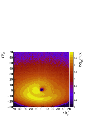
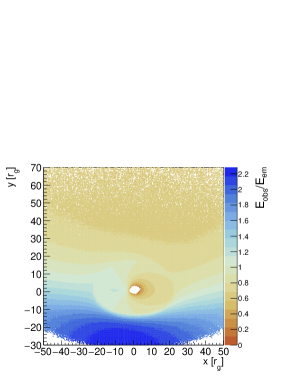
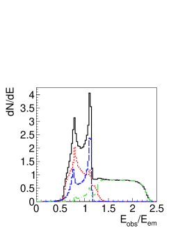
Figure 1: Intensity (left, logarithmic scale) and relative change of the photon energy between emission in the plasma frame and observation (center and right panels) of the reflected emission of a mass accreting Kerr black hole ($a=0.98$) driving a fast wind with an asymptotic velocity of 0.75 $c$. The results are shown for an observer at an inclination of 50^∘ relative to the spin axis of the black hole. In the right panel, the different line styles show the entire reflected emission (black solid line), and the emission reflected off (A) the far side of the wind (red dotted line), (B) the accretion disk at radial coordinates $r\,<\,20\,r_{\rm g}$ (blue dashed line), and (C) the near side of the wind (green dash-dotted line).

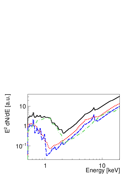
Figure 2: Spectral Energy Distribution (SED) of the reflected emission from the configuration of Figure 1 obtained with the xTrack ray tracing code and the XILLVER reflection code (García et al., 2014). See Figure 1 for the description of the different line styles.

Figures 1 and  2 shows the results from the simulation. The configuration leads to three major emission components (see the different line styles in Figure 1, right panel, and Figure 2). Component (A) comes from the far side of the conical outflow moving at an approximate angle $\theta_{\rm far}\,\approx\,i+\alpha=110$^∘relative to the observer. As the motion is mostly transverse to the line of sight, the emission is relativistically de-boosted by Doppler factors down to $\delta_{\rm far}=[\gamma_{\infty}(1-\beta_{\infty}\cos{\theta_{\rm far}})]^{-1}\approx\,$0.5, giving rise to emission between 3.5 keV and 5 keV. Component (B) comes mostly from the inner $<20$$\,r_{\rm g}$ region of the accretion flow. The emission from Component (C) comes from the near side of the flow moving towards the observer at an approximate observer frame angle of $\theta_{\rm near}\,\approx\,\alpha-i=10$^∘. The relativistic motion boosts the photon energy by Doppler factors up to $\delta_{\rm near}=[\gamma_{\infty}(1-\beta_{\infty}\cos{\theta_{\rm near}})]^{-1}\approx\,$2.5, giving rise to emission up to 16 keV. Figure 2 shows the resulting Spectral Energy Distribution (SED). The SED exhibits a rather broad excess with a subdued peak at 4 keV coming from the far side of the wind, a pronounced peak at 7 keV coming mostly from the approaching side of the accretion disk, and rather smooth excess emission between 7 keV and 16 keV coming from the near side of the wind. Fitting the model to actual data sets is outside of the scope of this paper.

4 Discussion

This paper presents a formalism that can be used to model inflows, outflows, and moving coronal plasma close to Kerr black holes. The formalism requires the flow velocity $\beta$ and angular velocity $\Omega$ of the plasma relative to a ZAMO. We show the results for an example where a generic parametrization is used for $\beta$, and $\Omega$ is inferred from angular momentum conservation. For future applications one could envision to use GR(R)MHD simulations or other physical inflow or outflow models to parameterize $\beta$ and $\Omega$.

We have shown in Section 3 that the approach can be used to model the reflection of coronal X-ray emission off an accretion disk and off a fast outflow. The self consistent modeling of the reflection off the two flow components makes it possible to predict not only the spectral shapes of the different reflection components, but also their relative intensities modulo uncertainties in the physical properties of the plasma. The calculations can furthermore predict the absolute and relative polarization and time offsets of the reflection components. Modeling of suitable data sets can be used to constrain not only the black hole spin and inclination, but also the physical properties and geometries of the reflectors.

The formalism can be used to analyze a wide range of phenomena:

1. Although plasma reaching the Innermost Stable Circular Orbit will plunge into the black hole, the emission cannot be neglected entirely (see Dovčiak et al., 2004; Noble et al., 2011; Kulkarni et al., 2011; Zhu et al., 2012). Recently, NICER and NuSTAR observations of the Galactic black hole X-ray binary MAXI J1820+070 show evidence for soft excess emission (Fabian et al., 2020). The authors speculate that magnetic stresses at the ISCO may explain the delayed infall and may power the emission. With suitable input from GR(R)MHD simulations, our formalism can be used to parametrize the motion of the plunging matter and to model the intensity and energy spectrum of the emission.

2. The accretion disks of black holes accreting at super-Eddington rates are expected to be geometrically thick, and the reflection of coronal emission off the funnel walls should lead to observable signatures (e.g. Brightman et al., 2019; Thomsen et al., 2019; Mundo et al., 2020). Along these lines, Kara et al. (2016) invoke the Fe K$\alpha$ emission from a relativistically moving upper accretion disk layer to explain the detection of a blue shifted iron lag from the tidal disruption event Swift J1644$+$57. The formalism introduced here can be used to quantitatively test models of the geometry and velocity of the flow by comparing the simulated with the predicted spectral and reverberation properties.

3. Observations of several Active Galactic Nuclei show strong evidence for a changing corona location or a changing corona geometry (e.g. Breedt et al., 2009; Parker et al., 2014; Wilkins & Gallo, 2015; Wilkins et al., 2015). Our formalism can be used to ascertain not only the impact of different corona geometries but also the impact of moderately or highly relativistic motion of the coronal plasma (see Reynolds & Fabian, 1997; Beloborodov, 1999; Fukumura & Kazanas, 2007). The emission from plasma moving relativistically towards the accretion disk can explain extremely high reflection ratios owing to the coronal emission being boosted in the direction of the disk. Conversely, plasma moving relativistically away from the accretion disk can explain extremely low reflection ratios owing to the deboosting of the coronal emission. The parameterization shown in this paper is not limited to describing motion along the spin axis of the black hole as in the earlier studies of Wilkins & Fabian (2012); Dauser et al. (2013).

4. The approach discussed here could also be used to simulate the emission, reflection, or reprocessing of radiation by non-axis-symmetric geometries. Karas et al. (2001); Hartnoll & Blackman (2002); Fukumura & Tsuruta (2004) for example consider the emission from accretion flows with spiral structure. Simulating non-axis-symmetric geometries will require to account for the azimuthal dependence of the flow geometry or the flow properties (e.g. the plasma density or the ionization degree).

Appendix

In this appendix, we give a rough estimate of the power required to drive an accretion disk wind as described in Section 3. The physical scale of system depends on the black hole mass and we do the estimate here for the $\sim 1.3\,\times\,10^{8}$ solar mass black hole of the quasar QSO J1131$-$1231 (Peng et al., 2006; Sluse et al., 2006; Dai et al., 2010; Sluse et al., 2012). The projected neutral hydrogen column density of the winds needs to be $\sim 10^{23}$  cm^-2. Assuming the photons impinge on the wind at the oblique angle $\alpha\,=\,60^{\circ}$, the Thomson optical depth is:

$$\tau_{\rm es}\,=\,1.2\,\frac{N_{\rm H}}{\cos{\alpha}}\,\sigma_{\rm T}\approx 16\%$$ (43)

with the factor 1.2 accounting for He atoms, and $\sigma_{\rm T}$ being the Thomson cross section. The corresponding K-shell photo-ionization optical depth for photons of energy $E_{\gamma}$ is (Ballantyne & Fabian, 2003):

$$\tau_{\rm FeK}(E_{\gamma})\,=\,\frac{N_{\rm H}}{\cos{\alpha}}\,A_{\rm Fe}\,\sigma_{K}(E_{\gamma}).$$ (44)

with $A_{\rm Fe}$ being the relative iron abundance, and $\sigma_{K}(E_{\gamma})$ the K-shell photoionization cross section from (Verner & Yakovlev, 1995). For a solar system iron abundance of $2.82\times 10^{-5}$, we get $\tau_{\rm FeK}\,=$ 19% and 8% for $E_{\gamma}=7.1$ keV and $E_{\gamma}=10$ keV, respectively. Neglecting the impact of electron scattering before and after the photoionization, the probability of a photon of energy $E_{\gamma}>7.1$ keV prompting the emission of an Fe K$\alpha$ photon into the hemisphere of the observer is given by (Ballantyne & Fabian, 2003):

$$P_{\rm FeK\alpha}(E_{\gamma})\,=\,\frac{1}{2}\,\omega\,b\,(1-e^{-\tau_{\rm FeK}(E_{\gamma})}).$$ (45)

The factor 1/2 gives the probability of emitting the Fe K$\alpha$ photon into the hemisphere of the observer, $\omega\,=\,0.342$ is the K fluorescence yield of iron, and $b\,=\,0.822$ is the K$\alpha$ to K$\beta$ branching ratio. The expressions gives a Fe K$\alpha$ yield of 2.5% and 1.1% for primary photons of 7.1 keV and 10 keV, respectively. If such a wind propagates at the distance $r_{\rm W}\,=30\,r_{\rm g}$ from the black hole’s spin axis with velocity $\beta$, the corresponding mass loss rate is in Newtonian approximation:

$$\dot{M}\,=\,\,N_{\rm H}\,\beta\,c\,2\pi\,30\,r_{\rm W}\,\frac{m_{\rm P}}{X_{\rm Sun}}$$ (46)

with $X_{\rm Sun}\,\approx\,0.74$ being the solar hydrogen mass fraction, and $m_{\rm P}$ the proton mass. Driving this outflow requires a mechanical luminosity of

$$L_{\rm wind}\,=\,(\gamma-1)\dot{M}c^{2}$$ (47)

with $\gamma=(1-\beta^{2})^{-1/2}$. For $\beta=0.25$, 0.5, and 0.75, the mechanical luminosity is 3%, 14%, and 46% of the Eddington Luminosity $L_{\rm Edd}$ of a 1.3$\times 10^{8}$ solar mass black hole. Note that $L_{\rm wind}$ and $L_{\rm Edd}$ both increase linearly with black hole mass, so that $L_{\rm wind}/L_{\rm Edd}$ is independent of the black hole mass.

References

- Abarr & Krawczynski (2020) Abarr, Q., & Krawczynski, H. 2020, ApJ,, 889, 111, doi: 10.3847/1538-4357/ab5fdf
- Abdikamalov et al. (2020) Abdikamalov, A. B., Ayzenberg, D., Bambi, C., et al. 2020, ApJ,, 899, 80, doi: 10.3847/1538-4357/aba625
- Ballantyne & Fabian (2003) Ballantyne, D. R., & Fabian, A. C. 2003, ApJ,, 592, 1089, doi: 10.1086/375798
- Bardeen et al. (1972) Bardeen, J. M., Press, W. H., & Teukolsky, S. A. 1972, ApJ,, 178, 347, doi: 10.1086/151796
- Beheshtipour et al. (2017) Beheshtipour, B., Krawczynski, H., & Malzac, J. 2017, ApJ,, 850, 14, doi: 10.3847/1538-4357/aa906a
- Beloborodov (1999) Beloborodov, A. M. 1999, ApJ,, 510, L123, doi: 10.1086/311810
- Blandford et al. (2019) Blandford, R., Meier, D., & Readhead, A. 2019, ARA&A,, 57, 467, doi: 10.1146/annurev-astro-081817-051948
- Blandford (1976) Blandford, R. D. 1976, MNRAS,, 176, 465, doi: 10.1093/mnras/176.3.465
- Blandford & Begelman (1999) Blandford, R. D., & Begelman, M. C. 1999, MNRAS,, 303, L1, doi: 10.1046/j.1365-8711.1999.02358.x
- Blandford & Payne (1982) Blandford, R. D., & Payne, D. G. 1982, MNRAS,, 199, 883, doi: 10.1093/mnras/199.4.883
- Breedt et al. (2009) Breedt, E., Arévalo, P., McHardy, I. M., et al. 2009, MNRAS,, 394, 427, doi: 10.1111/j.1365-2966.2008.14302.x
- Brightman et al. (2019) Brightman, M., Bachetti, M., Earnshaw, H. P., et al. 2019, BAAS,, 51, 352. https://arxiv.org/abs/1903.06844
- Broderick & Blandford (2004) Broderick, A., & Blandford, R. 2004, MNRAS,, 349, 994, doi: 10.1111/j.1365-2966.2004.07582.x
- Bronzwaer et al. (2020) Bronzwaer, T., Younsi, Z., Davelaar, J., & Falcke, H. 2020, A&A,, 641, A126, doi: 10.1051/0004-6361/202038573
- Chartas et al. (2017) Chartas, G., Krawczynski, H., Zalesky, L., et al. 2017, ApJ,, 837, 26, doi: 10.3847/1538-4357/aa5d50
- Choudhury et al. (2017) Choudhury, K., García, J. A., Steiner, J. F., & Bambi, C. 2017, ApJ,, 851, 57, doi: 10.3847/1538-4357/aa9925
- Cocke & Holm (1972) Cocke, W. J., & Holm, D. A. 1972, Nature Physical Science, 240, 161, doi: 10.1038/physci240161b0
- Dai et al. (2010) Dai, X., Kochanek, C. S., Chartas, G., et al. 2010, ApJ,, 709, 278, doi: 10.1088/0004-637X/709/1/278
- Dauser et al. (2013) Dauser, T., Garcia, J., Wilms, J., et al. 2013, MNRAS,, 430, 1694, doi: 10.1093/mnras/sts710
- Davis & Gammie (2020) Davis, S. W., & Gammie, C. F. 2020, ApJ,, 888, 94, doi: 10.3847/1538-4357/ab5950
- Dexter (2016) Dexter, J. 2016, MNRAS,, 462, 115, doi: 10.1093/mnras/stw1526
- Dovčiak et al. (2004) Dovčiak, M., Karas, V., & Yaqoob, T. 2004, ApJS,, 153, 205, doi: 10.1086/421115
- Fabian et al. (2020) Fabian, A. C., Buisson, D. J., Kosec, P., et al. 2020, MNRAS,, 493, 5389, doi: 10.1093/mnras/staa564
- Fukumura & Kazanas (2007) Fukumura, K., & Kazanas, D. 2007, ApJ,, 664, 14, doi: 10.1086/518883
- Fukumura et al. (2010) Fukumura, K., Kazanas, D., Contopoulos, I., & Behar, E. 2010, ApJ,, 723, L228, doi: 10.1088/2041-8205/723/2/L228
- Fukumura & Tsuruta (2004) Fukumura, K., & Tsuruta, S. 2004, ApJ,, 613, 700, doi: 10.1086/423312
- Gammie & Leung (2012) Gammie, C. F., & Leung, P. K. 2012, ApJ,, 752, 123, doi: 10.1088/0004-637X/752/2/123
- García et al. (2014) García, J., Dauser, T., Lohfink, A., et al. 2014, ApJ,, 782, 76, doi: 10.1088/0004-637X/782/2/76
- Gold et al. (2020) Gold, R., Broderick, A. E., Younsi, Z., et al. 2020, ApJ,, 897, 148, doi: 10.3847/1538-4357/ab96c6
- Hartnoll & Blackman (2002) Hartnoll, S. A., & Blackman, E. G. 2002, MNRAS,, 332, L1, doi: 10.1046/j.1365-8711.2002.05405.x
- Higginbottom et al. (2014) Higginbottom, N., Proga, D., Knigge, C., et al. 2014, ApJ,, 789, 19, doi: 10.1088/0004-637X/789/1/19
- Hoormann et al. (2016) Hoormann, J. K., Beheshtipour, B., & Krawczynski, H. 2016, Phys. Rev. D,, 93, 044020, doi: 10.1103/PhysRevD.93.044020
- Kara et al. (2016) Kara, E., Miller, J. M., Reynolds, C., & Dai, L. 2016, Nature,, 535, 388, doi: 10.1038/nature18007
- Karas et al. (2001) Karas, V., Martocchia, A., & Subr, L. 2001, PASJ,, 53, 189, doi: 10.1093/pasj/53.2.189
- Kinch et al. (2019) Kinch, B. E., Schnittman, J. D., Kallman, T. R., & Krolik, J. H. 2019, ApJ,, 873, 71, doi: 10.3847/1538-4357/ab05d5
- Krawczynski (2012) Krawczynski, H. 2012, ApJ,, 754, 133, doi: 10.1088/0004-637X/754/2/133
- Krawczynski et al. (2019) Krawczynski, H., Chartas, G., & Kislat, F. 2019, ApJ,, 870, 125, doi: 10.3847/1538-4357/aaf39c
- Kulkarni et al. (2011) Kulkarni, A. K., Penna, R. F., Shcherbakov, R. V., et al. 2011, MNRAS,, 414, 1183, doi: 10.1111/j.1365-2966.2011.18446.x
- Li et al. (2005) Li, L.-X., Zimmerman, E. R., Narayan, R., & McClintock, J. E. 2005, ApJS,, 157, 335, doi: 10.1086/428089
- Liska et al. (2020) Liska, M., Hesp, C., Tchekhovskoy, A., et al. 2020, MNRAS,, doi: 10.1093/mnras/staa099
- Matt et al. (1991) Matt, G., Perola, G. C., & Piro, L. 1991, A&A,, 247, 25
- Miller et al. (2015) Miller, J. M., Fabian, A. C., Kaastra, J., et al. 2015, ApJ,, 814, 87, doi: 10.1088/0004-637X/814/2/87
- Misner et al. (2017) Misner, C. W., Thorne, K. S., & Wheeler, J. A. 2017, Gravitation (Princeton University Press)
- Mościbrodzka & Gammie (2018) Mościbrodzka, M., & Gammie, C. F. 2018, MNRAS,, 475, 43, doi: 10.1093/mnras/stx3162
- Mundo et al. (2020) Mundo, S. A., Kara, E., Cackett, E. M., et al. 2020, MNRAS,, 496, 2922, doi: 10.1093/mnras/staa1744
- Noble et al. (2011) Noble, S. C., Krolik, J. H., Schnittman, J. D., & Hawley, J. F. 2011, ApJ,, 743, 115, doi: 10.1088/0004-637X/743/2/115
- Nomura & Ohsuga (2017) Nomura, M., & Ohsuga, K. 2017, MNRAS,, 465, 2873, doi: 10.1093/mnras/stw2877
- Page & Thorne (1974) Page, D. N., & Thorne, K. S. 1974, ApJ,, 191, 499, doi: 10.1086/152990
- Parker et al. (2014) Parker, M. L., Wilkins, D. R., Fabian, A. C., et al. 2014, Monthly Notices of the Royal Astronomical Society, 443, 1723, doi: 10.1093/mnras/stu1246
- Peng et al. (2006) Peng, C. Y., Impey, C. D., Rix, H.-W., et al. 2006, ApJ,, 649, 616, doi: 10.1086/506266
- Porth et al. (2019) Porth, O., Chatterjee, K., Narayan, R., et al. 2019, ApJS,, 243, 26, doi: 10.3847/1538-4365/ab29fd
- Reynolds & Fabian (1997) Reynolds, C. S., & Fabian, A. C. 1997, MNRAS,, 290, L1, doi: 10.1093/mnras/290.1.L1
- Schnittman & Krolik (2009) Schnittman, J. D., & Krolik, J. H. 2009, ApJ,, 701, 1175, doi: 10.1088/0004-637X/701/2/1175
- Schnittman & Krolik (2010) —. 2010, ApJ,, 712, 908, doi: 10.1088/0004-637X/712/2/908
- Sluse et al. (2012) Sluse, D., Hutsemékers, D., Courbin, F., Meylan, G., & Wambsganss, J. 2012, A&A,, 544, A62, doi: 10.1051/0004-6361/201219125
- Sluse et al. (2006) Sluse, D., Claeskens, J. F., Altieri, B., et al. 2006, A&A,, 449, 539, doi: 10.1051/0004-6361:20053148
- Tamborra et al. (2018) Tamborra, F., Matt, G., Bianchi, S., & Dovčiak, M. 2018, A&A,, 619, A105, doi: 10.1051/0004-6361/201732023
- Thomsen et al. (2019) Thomsen, L. L., Lixin Dai, J., Ramirez-Ruiz, E., Kara, E., & Reynolds, C. 2019, ApJ,, 884, L21, doi: 10.3847/2041-8213/ab4518
- Verner & Yakovlev (1995) Verner, D. A., & Yakovlev, D. G. 1995, A&AS,, 109, 125
- Waters et al. (2016) Waters, T., Kashi, A., Proga, D., et al. 2016, The Astrophysical Journal, 827, 53, doi: 10.3847/0004-637x/827/1/53
- Wilkins & Fabian (2012) Wilkins, D. R., & Fabian, A. C. 2012, MNRAS,, 424, 1284, doi: 10.1111/j.1365-2966.2012.21308.x
- Wilkins & Gallo (2015) Wilkins, D. R., & Gallo, L. C. 2015, MNRAS,, 449, 129, doi: 10.1093/mnras/stv162
- Wilkins et al. (2015) Wilkins, D. R., Gallo, L. C., Grupe, D., et al. 2015, MNRAS,, 454, 4440, doi: 10.1093/mnras/stv2130
- Yuan & Narayan (2014) Yuan, F., & Narayan, R. 2014, ARA&A,, 52, 529, doi: 10.1146/annurev-astro-082812-141003
- Zhang et al. (2019) Zhang, W., Dovčiak, M., & Bursa, M. 2019, ApJ,, 875, 148, doi: 10.3847/1538-4357/ab1261
- Zhu et al. (2012) Zhu, Y., Davis, S. W., Narayan, R., et al. 2012, MNRAS,, 424, 2504, doi: 10.1111/j.1365-2966.2012.21181.x