Proximal Policy Gradient: PPO with Policy Gradient

Abstract

In this paper, we propose a new algorithm PPG (Proximal Policy Gradient), which is close to both VPG (vanilla policy gradient) and PPO (proximal policy optimization). The PPG objective is a partial variation of the VPG objective and the gradient of the PPG objective is exactly same as the gradient of the VPG objective. To increase the number of policy update iterations, we introduce the advantage-policy plane and design a new clipping strategy. We perform experiments in OpenAI Gym and Bullet robotics environments for ten random seeds. The performance of PPG is comparable to PPO, and the entropy decays slower than PPG. Thus we show that performance similar to PPO can be obtained by using the gradient formula from the original policy gradient theorem.

Introduction

Policy gradient algorithms introduced in (Williams 1992; Sutton et al. 2000a, b) compute the gradient of the expected return with respect to policy parameters. An action-independent term, typically the state value function, can be subtracted from this gradient. Then, the policy gradient is in the form of gradient of log probability multiplied by the advantage function. The resulting policy gradient algorithm respectively boosts (reduces), the probability of advantageous (disadvantageous) actions. This policy gradient algorithm is too slow to be used as a modern day baseline. Therefore, a reasonable choice of recent advances are applied to the classic policy gradient theorem based methods. In (Achiam 2018), the generalized advantage estimate (GAE) (Schulman et al. 2015b) and the advantage normalization are applied. The resulting algorithm is called the Vanilla Policy Gradient (VPG) (Achiam 2018; Dhariwal et al. 2017).

Recently, the trust region policy optimization (TRPO) (Schulman et al. 2015a) and the proximal policy optimization (PPO) (Schulman et al. 2017) present significant performance improvement over VPG by using the proposed surrogate objective function. In particular, PPO is very popular due to the learning stability and implementation simplicity. PPO provides a novel solution to the problem of increasing the number of policy updates by introducing the clipping idea. In practice, the number of iterations cannot be indefinitely large. Instead, the iteration continues until a target KL divergence is reached. Thus a much larger number of policy update iterations per each roll out is possible, greatly increasing the sample efficiency while maintaining the steady improvement on the average return. This is the baseline PPO algorithm we use to perform experiments. Note that there are variety of variations of PPO (Schulman et al. 2017) for various enhancements.

We explore a slight modification to both VPG and PPO, devise an objective that appears to be in between, and study the performance. The objective without clipping has the gradient exactly the same as VPG’s gradient. This objective can be considered as a partial variation of the VPG objective, i.e., PPG optimizes the changes of the VPG objective. In contrast, PPO optimizes the expected importance-weighted advantage, and hence, the gradient of the PPO objective is different from VPG, which is based on the policy gradient theorem (Sutton et al. 2000a). To achieve performance similar to PPO, we introduce a new clipping algorithm designed for the PPG objective. The clipping is applied to samples that have their probabilities adjusted enough, so that these samples are excluded from the training batch.

We perform experiments in the popular continuous control environments in OpenAI Gym (Brockman et al. 2016) with the MuJoCo simulator: Ant, HalfCheetah, Hopper, and Walker2d, and also in the corresponding Bullet environments: AntBulletEnv, HalfCheetahBulletEnv, HopperBulletEnv, and Walker2DBulletEnv. We found that PPG and PPO are very similar with a few cases where PPG appears to have marginally higher average returns. The entropy tends to decay slower in PPG than in PPO. Therefore, PPG solutions appear to be more stochastic than PPO solutions. Thus, we show that policy gradient can be used for the PPO algorithm.

Related Work

Model free reinforcement learning algorithms have evolved from the classic dynamic programming, policy and value iterations (Sutton and Barto 2018) to Q-learning (Watkins 1989) and direct policy search methods using neural networks for policy and value functions (Mnih et al. 2015, 2016; Andrychowicz et al. 2018; Lillicrap et al. 2015; Fujimoto et al. 2018; Haarnoja et al. 2018).

On-policy algorithms are popular for their stability, i.e., applicability to a wide set of problems. One of the early on-policy policy-gradient based methods is REINFORCE (Williams 1992) that directly used Monte-Carlo returns. Instead, value estimate was used in the Actor-Critic method (Sutton et al. 1999). In modern days, value estimates are frequently formulated as advantages. To reduce the noise in advantage, the generalized advantage estimation method has been proposed in (Schulman et al. 2015b).

The policy-gradient theorem (Sutton et al. 2000a) is used to compute the gradient of expected return in terms of policy parameters. This gradient is formulated as an objective function, which is handed over to an optimizer with an auto-derivative support. A reasonable implementation of this algorithm is called VPG (Achiam 2018; Dhariwal et al. 2017). On the other hand, TRPO (Schulman et al. 2015a) and PPO (Schulman et al. 2017) use the surrogate objective. TRPO uses natural policy gradient with KL divergence constraints while PPO uses a simple clipping mechanism. Despite the simplicity, PPO often outperforms TRPO.

The performance of PPO can be improved by a variety of secondary optimization techniques. For example, value function clipping and reward scaling have been studied in (Engstrom et al. 2020), where these secondary optimizations are shown to be crucial for PPO’s performance. Since the success of model-free algorithms depends on its exploration and PPO tends to not sufficiently explore, Wang et al. (2019) proposed to adjust the clipping range within the trust region to encourage the exploration. The performance of PPO is also enormously influenced by its entropy. Ahmed et al. (2019) and Liu et al. (2019) present higher entropy can be utilized as a regularizer that produces smoother training results.

In this paper, we choose a PPO implementation with clipping and KL divergence break, and then study whether the original policy gradient theorem can be used instead of the surrogate objective, and still performance similar to PPO can be obtained.

Policy Optimization Objectives

In this section, we first define the objectives of VPG, PPO, and PPG, and provide the detailed discussions in the later sections.

VPG: Vanilla Policy Gradient

Policy Gradient (PG) methods, originally developed in (Williams 1992; Sutton et al. 2000b), are to update a parameterized policy by ascending along the stochastic gradient of the expected return. The gradient of PG has the form

$$\nabla_{\theta}J(\pi_{\theta})=\mathbb{E}_{\pi_{\theta}}\bigg{[}\nabla_{\theta}\log\pi_{\theta}(a_{t}|s_{t})A^{\pi}(s_{t},a_{t})\bigg{]},$$ (1)

where $\pi_{\theta}$ is a stochastic policy with the parameter $\theta$. $A^{\pi}$ is commonly referred to as the advantage function $A^{\pi}(s_{t},a_{t})=Q^{\pi}(s_{t},a_{t})-V^{\pi}(s_{t})$ where $Q^{\pi}(s_{t},a_{t})$ is a state-action value function and $V^{\pi}(s_{t})$ is a state value function. Since this advantage $A^{\pi}_{t}$ is noisy, the generalized advantage estimation (Schulman et al. 2015b) is applied to reduce the variance. We denote the resulting advantage as $A_{t}^{GAE}$. Finally, we normalize $A_{t}^{GAE}$ and compute the normalized advantage $\hat{A}_{t}$ such that the mean is zero and the standard deviation is 1. We exploit this $\hat{A}_{t}$ to define the objective of VPG, denoted as $L^{\scalebox{0.55}{$VPG$}}$.

$$L^{\scalebox{0.55}{$VPG$}}=\frac{1}{\hat{N}}\sum_{i,t=1}^{N,T_{i}}\log\pi_{\theta}(a_{i,t}|s_{i,t})\hat{A}_{t}.$$ (2)

where $N$ is the number of episodes in the roll out, $T_{i}$ is the time steps in episode $i$, and $\hat{N}=\sum T_{i}$ is the size of the roll out.

PPO: Proximal Policy Optimization

Proximal Policy Optimization (PPO) (Schulman et al. 2017) and TRPO (Wang et al. 2019) use the surrogate objective (Zhang, Wu, and Pineau 2018; Schulman et al. 2015a).

$$\begin{split}&\underset{\theta}{\mathrm{maximize}}\;\mathbb{E}_{t}\bigg{[}\frac{\pi_{\theta}(a_{t}|s_{t})}{\pi_{\theta_{old}}(a_{t}|s_{t})}\hat{A}_{t}\bigg{]}\\ &\text{subject to}\;\mathbb{E}_{t}\bigg{[}D_{KL}\left(\pi_{\theta}(\cdot|s_{t})||\pi_{\theta_{old}}(\cdot|s_{t})\right)\bigg{]}\leq\delta\end{split}$$ (3)

To avoid the high computational cost and implementation complexity of TRPO, PPO proposes simple techniques: clipped surrogate objective or adaptive KL penalty (Schulman et al. 2017).

Among many variations of PPO, we select an OpenAI’s implementation found in (Achiam 2018). The loss objective of PPO using the clipped surrogate objective method is $L^{\scalebox{0.55}{$PPO$}}$ in (4). We also provide the objective without clipping $L^{\scalebox{0.55}{$PPO$}}_{\scalebox{0.55}{$NCLIP$}}$.

$$\begin{split}&L^{\scalebox{0.55}{$PPO$}}_{\scalebox{0.55}{$NCLIP$}}=\frac{1}{\hat{N}}\sum_{i,t=1}^{N,T_{i}}r_{i,t}(\theta)\hat{A}_{t}\\ &L^{\scalebox{0.55}{$PPO$}}=\frac{1}{\hat{N}}\sum_{i,t=1}^{N,T_{i}}\mathrm{min}(r_{i,t}(\theta),\mathrm{clip}(r_{i,t}(\theta),1\pm\epsilon))\hat{A}_{t}\\ &\qquad\;\text{where}\;r_{i,t}(\theta)=\pi_{\theta}(a_{i,t}|s_{i,t})\;/\;\pi_{\theta_{old}}(a_{i,t}|s_{i,t})\end{split}$$ (4)

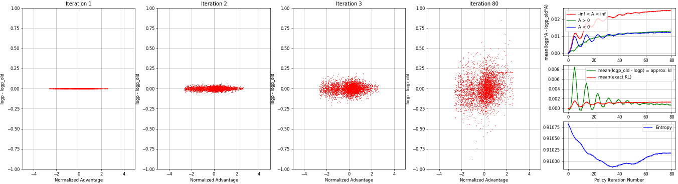
Figure 1: Typical PPG policy iterations from AntBulletEnv training with roll out size of 4000. At the beginning of the iteration, all samples are in the $x$ axis as $\log\pi_{i}-\log\pi_{i_{\mbox{old}}}=0$. As iteration continues, policy is updated, and $\log\pi_{i}-\log\pi_{i_{\mbox{old}}}$ changes. In the far right, we show the objective changes in top (green for positive advantages, blue for negative advantages, and red for all), KL divergences in the middle (green for approximate KL and red for the average exact KL), and entropy changes in the bottom.

PPG: Proximal Policy Gradient

PPG, which we propose in this paper, is a simple variant of VPG, or a simple variant of PPO. We design the objective so that its gradient is the same as the gradient of $L^{\scalebox{0.55}{$VPG$}}$, while a clipping method similar to PPO is applicable. The resulting form has the log probability difference between the current policy and the old policy, $d_{i,t}(\theta)=\log\pi_{\theta}(a_{i,t}|s_{i,t})-\log\pi_{\theta_{old}}(a_{i,t}|s_{i,t})$. This can also be interpreted as the application of the logarithmic operation to the surrogate objective as $d_{i,t}=\log r_{i,t}$. The objectives without clipping $L^{\scalebox{0.55}{$PPG$}}_{\scalebox{0.55}{$NCLIP$}}$ and with clipping $L^{\scalebox{0.55}{$PPG$}}$ are

$$\begin{split}&L^{\scalebox{0.55}{$PPG$}}_{\scalebox{0.55}{$NCLIP$}}=\frac{1}{\hat{N}}\sum_{i,t=1}^{N,T_{i}}d_{i,t}(\theta)\hat{A}_{t},\\ &L^{\scalebox{0.55}{$PPG$}}=\frac{1}{\hat{N}}\sum_{i,t=1}^{N,T_{i}}\hat{A}_{t}\;\delta_{i,t}(\theta),\\ &\quad\delta_{i,t}(\theta)=\left\{\begin{array}[]{ll}\min(d_{i,t}(\theta),u_{b}),\;\hat{A}_{t}\geq 0\\ \max(d_{i,t}(\theta),l_{b}),\;\hat{A}_{t}<0\end{array}\right.,\\ &\quad d_{i,t}(\theta)=\log\pi_{\theta}(a_{i,t}|s_{i,t})-\log\pi_{\theta_{old}}(a_{i,t}|s_{i,t}),\\ &\quad u_{b}\;\text{is the clipping upper bound constant,}\\ &\quad l_{b}\;\text{is the clipping lower bound constant.}\\ \end{split}$$ (5)

Note that this clipping depends on the sign of the advantage $\hat{A}_{t}$. For the design details of $L^{\scalebox{0.55}{$PPG$}}$, we defer the discussion to the next section.

Since $\pi_{\theta_{old}}$ is a constant, the derivative of the $L^{\scalebox{0.55}{$PPG$}}_{\scalebox{0.55}{$NCLIP$}}$ is exactly equal to $L^{\scalebox{0.55}{$VPG$}}$, which is based on the gradient from the policy gradient theorem. Also note that the gradient of $L^{\scalebox{0.55}{$PPO$}}_{\scalebox{0.55}{$NCLIP$}}$ is different from $L^{\scalebox{0.55}{$VPG$}}$.

$$\begin{split}\nabla_{\theta}L^{\scalebox{0.55}{$PPG$}}_{\scalebox{0.55}{$NCLIP$}}&=\nabla_{\theta}L^{\scalebox{0.55}{$VPG$}}=\frac{1}{\hat{N}}\sum_{i,t=1}^{N,T_{i}}\nabla_{\theta}\log\pi_{\theta}(a_{i,t}|s_{i,t})\hat{A}_{t}\\ &\neq\nabla_{\theta}L^{\scalebox{0.55}{$PPO$}}_{\scalebox{0.55}{$NCLIP$}}=\frac{1}{\hat{N}}\sum_{i,t=1}^{N,T_{i}}\frac{\nabla_{\theta}\pi_{\theta}(a_{i,t}|s_{i,t})}{\pi_{\theta_{old}}(a_{i,t}|s_{i,t})}\hat{A}_{t}\end{split}$$

The samples clipped by (5) do not contribute to the gradient of $L^{\scalebox{0.55}{$PPG$}}$, and hence, for unclipped samples, $\nabla_{\theta}L^{\scalebox{0.55}{$PPG$}}=\nabla_{\theta}L^{\scalebox{0.55}{$PPG$}}_{\scalebox{0.55}{$NCLIP$}}=\nabla_{\theta}L^{\scalebox{0.55}{$VPG$}}$.

PPG Clipping in Advantage Policy Plane

When training a policy using VPG, it is difficult to match the performance of PPO simply by increasing the number of iteration as shown in Fig. 2. In order to achieve similar performance of PPO, a clipping mechanism similar to PPO is needed. In this section, we develop this clipping formula $L^{\scalebox{0.55}{$PPG$}}$ in (5), which we call PPG clipping.

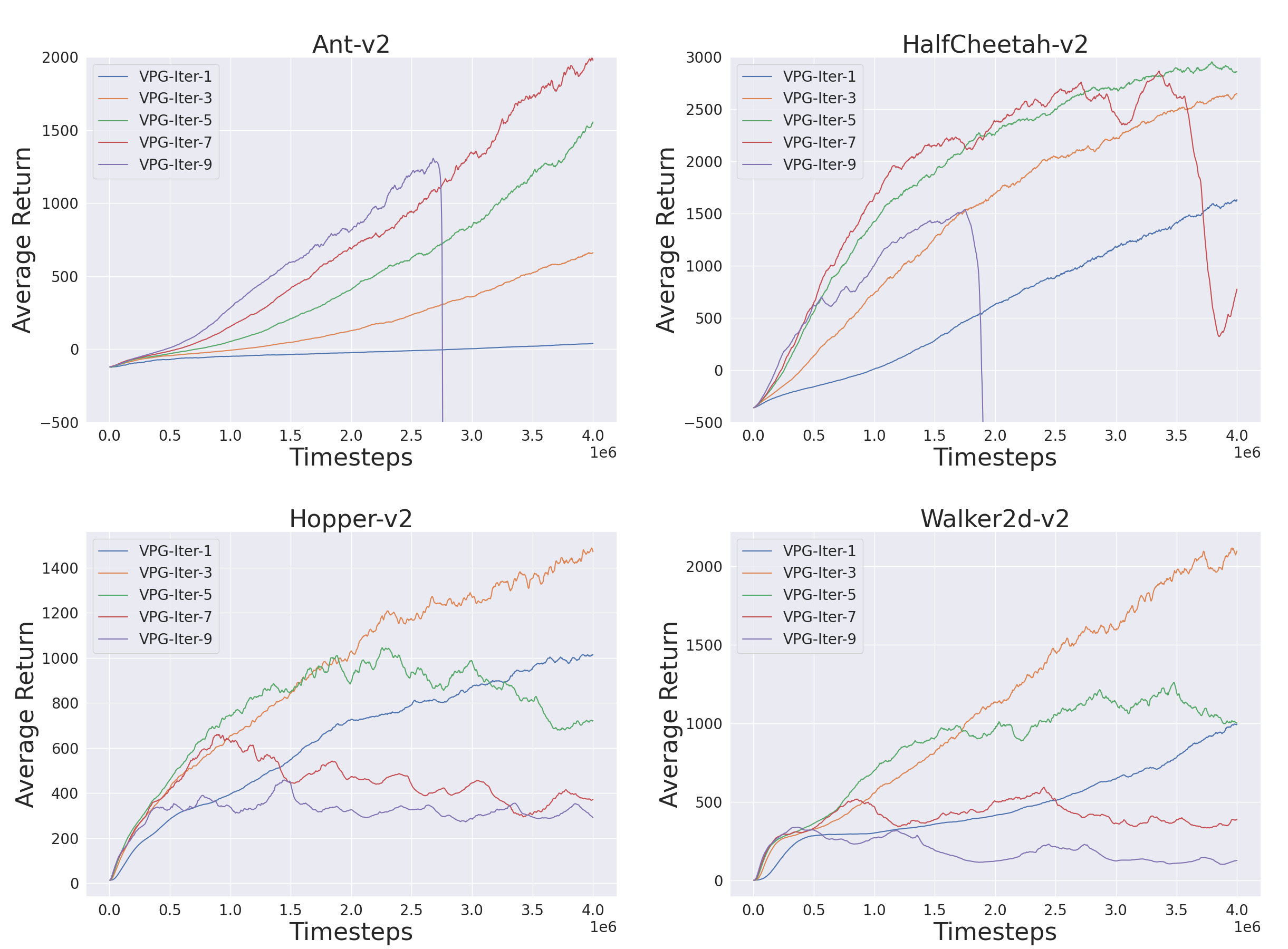
Figure 2: Results from multiple VPG policy iterations are exactly the same as PPG iterations without clipping, i.e., optimizing with $L^{\scalebox{0.55}{$PPG$}}_{\scalebox{0.55}{$NCLIP$}}$. Simply increasing the number of VPG policy iterations can result in eventual failures. Even for iterations that do not demonstrate a failure in this experiment, a failure can happen later if the training is continued.

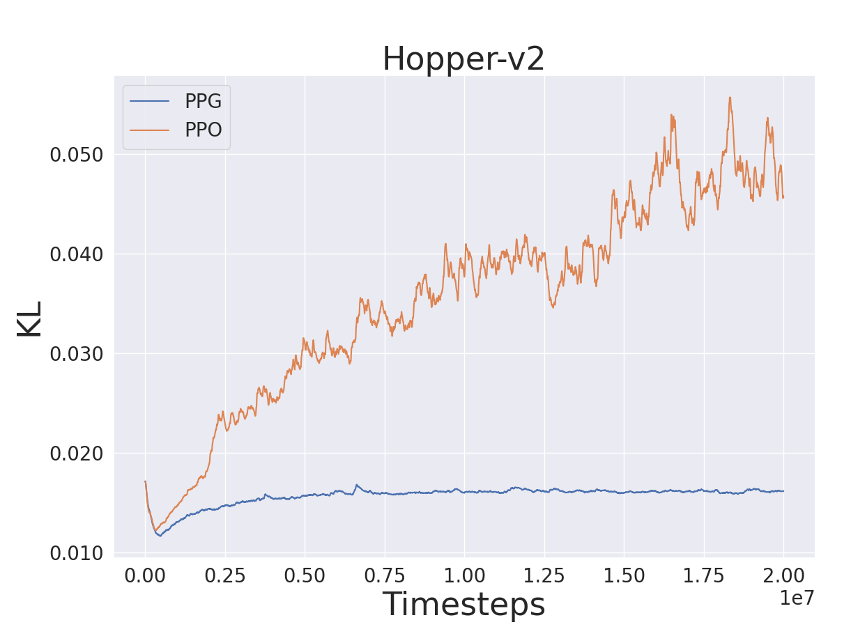
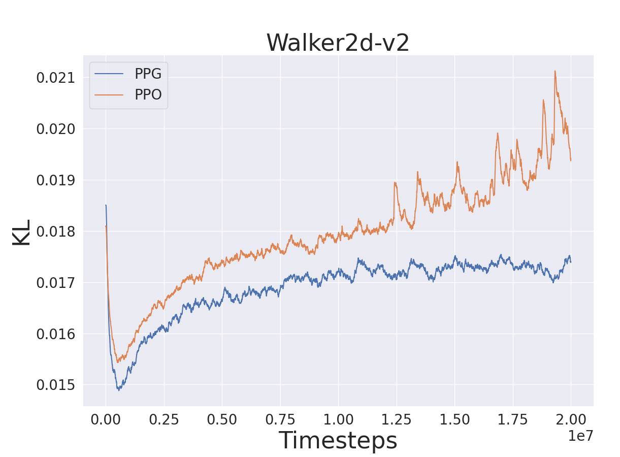
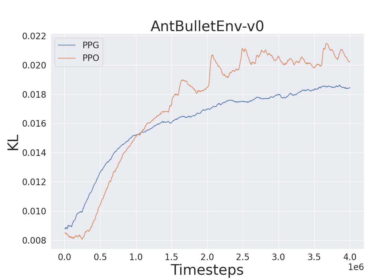
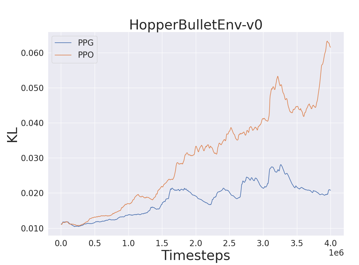
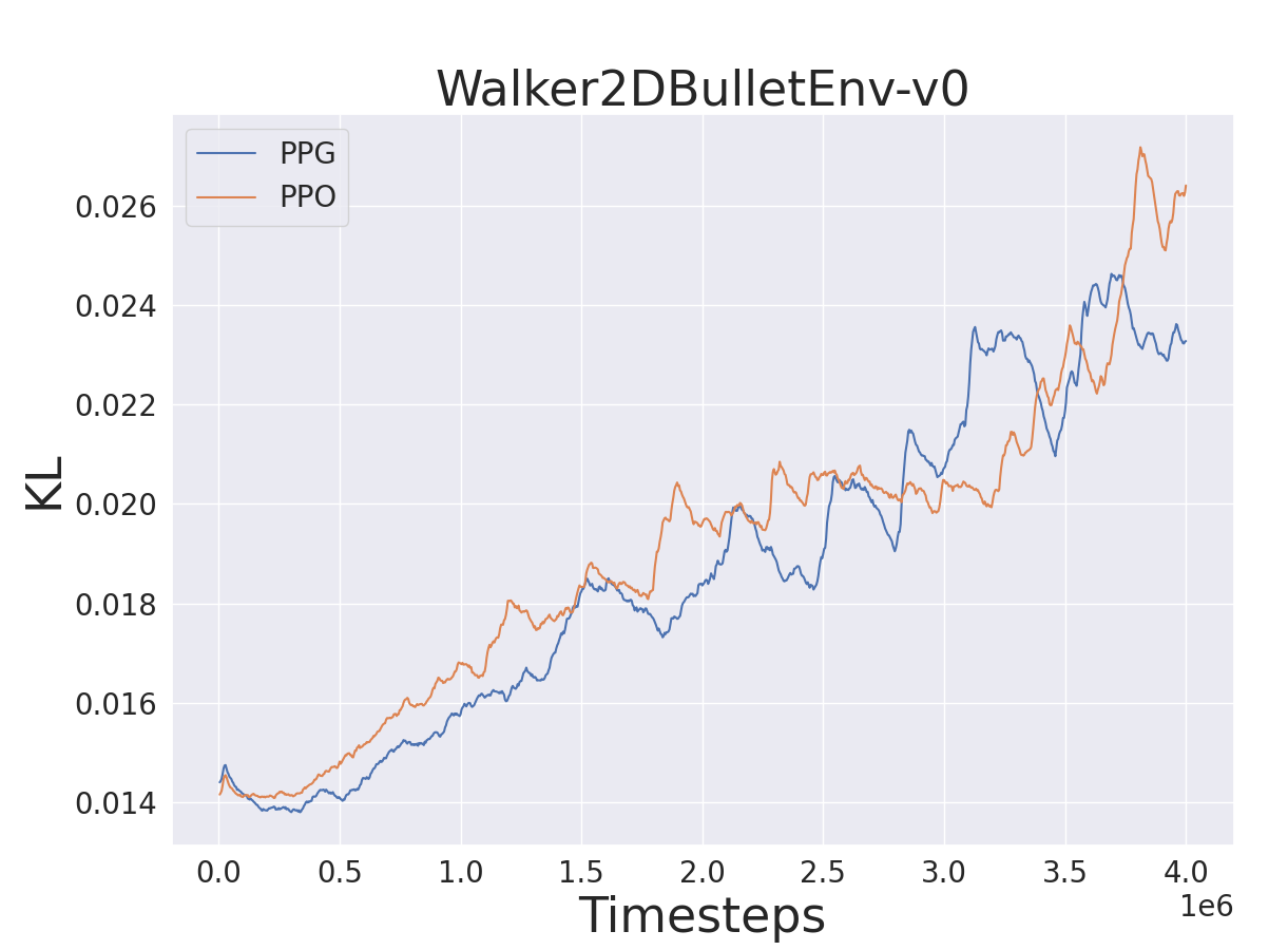
Figure 3: KL divergences for PPG (light blue) and PPO (light orange). The graphs show the KL divergences of PPG tend to stay lower than that of PPO throughout the training.

Figure 4: Advantage-Policy plane. In left half plane, since $\hat{A}_{t}<0$, probability should decrease and on the right half plane, since $\hat{A}_{t}>0$, probability should increase. We apply a clipping such that gradient is zero in the blue shaded regions since log probabilities have updated more than the clipping thresholds $u_{b}$ and $l_{b}$. See Fig. 1 for an example.

In a policy update iteration, if $\hat{A}_{t}>0$, the policy parameters should be updated to increase the probability $\pi_{\theta}(a_{t}|s_{t})$, and if $\hat{A}_{t}<0$, the policy parameters should be updated in the direction of decreasing $\pi_{\theta}(a_{t}|s_{t})$. As illustrated in Fig. 4, the gradient of $L^{\scalebox{0.55}{$PPG$}}$ should have a downward $y$-component in the $2^{nd}$ and the $3^{rd}$ quadrants, and a upward $y$-component in the $1^{st}$ and the $4^{th}$ quadrants.

Suppose a sample is in the $2^{nd}$ quadrant. This means that the probability has been increased even though the action is disadvantageous. To penalize this undesirable update, we do not set a clipping upper bound. Then all samples in the $2^{nd}$ quadrant are used in the gradient ascent, and their probabilities are likely to be decreased for the next policy update. Now, suppose that a sample is in the $4^{th}$ quadrant. This represents that the probability of that advantageous action is decreased. Therefore, the objective function should not clip the sample to penalize all of such cases.

Samples in the $1^{st}$ quadrant indicate that probabilities of advantageous actions are increased. These samples are updated properly unless the amount of log probability increase is too much. Therefore, we set an upper bound to prevent the policy from being too deterministic. Samples above this bound will have zero gradient, and hence are not forced to increase the probability further. This procedure also similarly works for samples in the $3^{rd}$ quadrant. The lower bound in the $3^{rd}$ quadrant prevents excessive probability decreases by forcing the gradients to be zero for all samples that the difference log probabilities is lower than the lower bound. Notice that clipped samples have zero gradient, so the samples in the desirable areas are effectively removed from the next policy update iteration. Thus the clipping makes the per iteration batch size small and only focuses on the samples that should be reflected in the next update.

In practice, as shown in Fig. 1, at the beginning of the policy iteration, all samples are in the $x$ axis, and as iteration continues, samples start spreading into all the quadrants. Although a large number of samples exist in the $2^{nd}$ and the $4^{th}$ quadrants, the objective function (the red lines top far right image in Fig. 1) indeed increases. A clip line ($u_{b}=0.2$) is sometimes observable as shown in the iteration 80. The iteration can be continued further until both of the clip lines are clearly observable, however, this typically hampers the performance.

Finally, we would like to note that one can design a variety of different clipping strategies such as slopped clip lines. In our tests, we obtained mixed results depending on environments. Thus, we left the exploration as a future work.

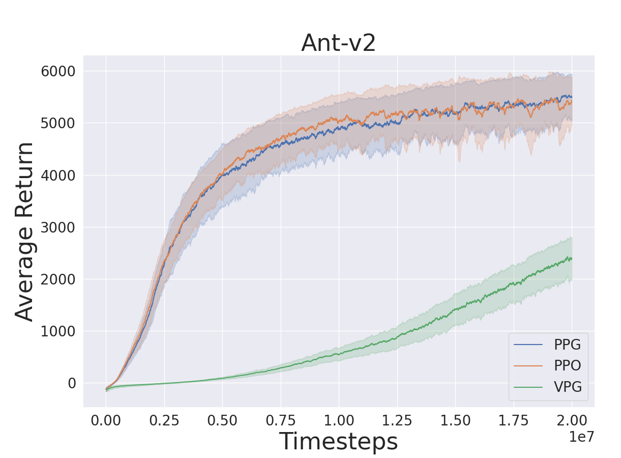
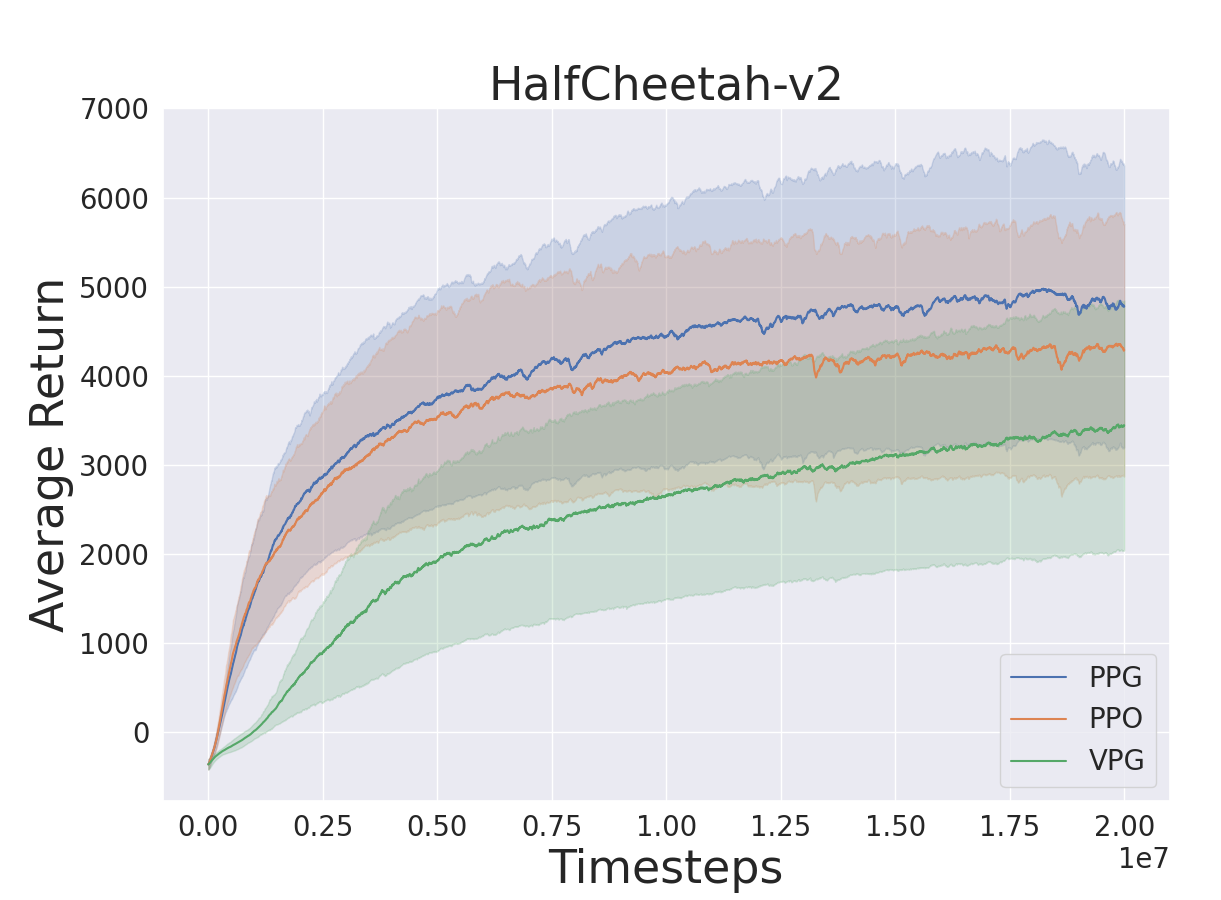
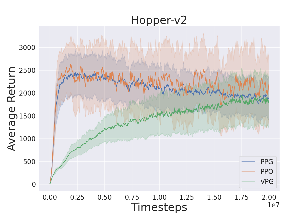
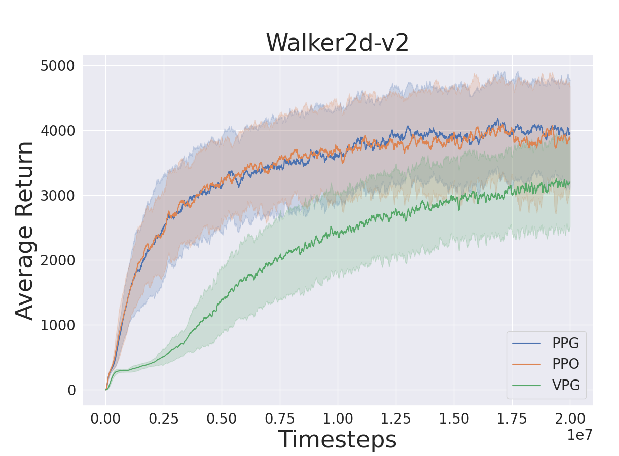
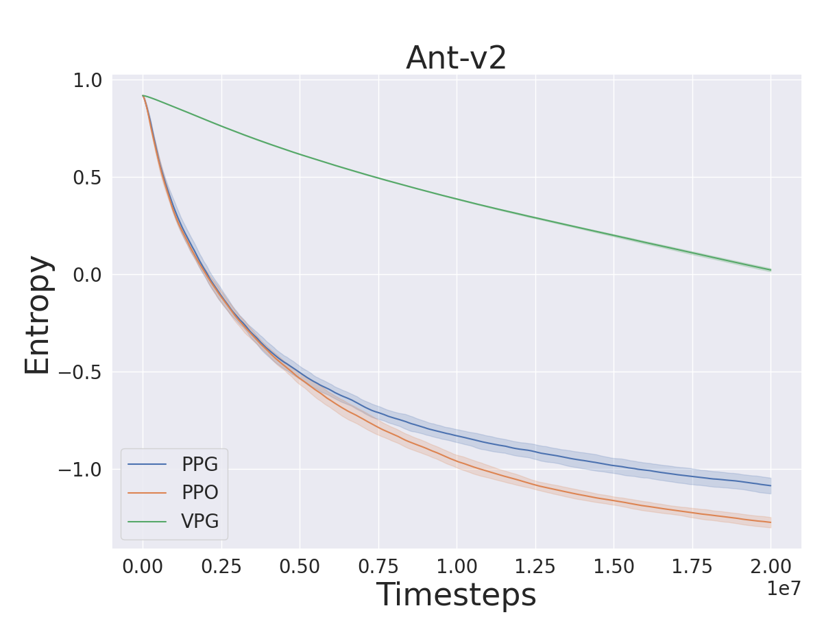
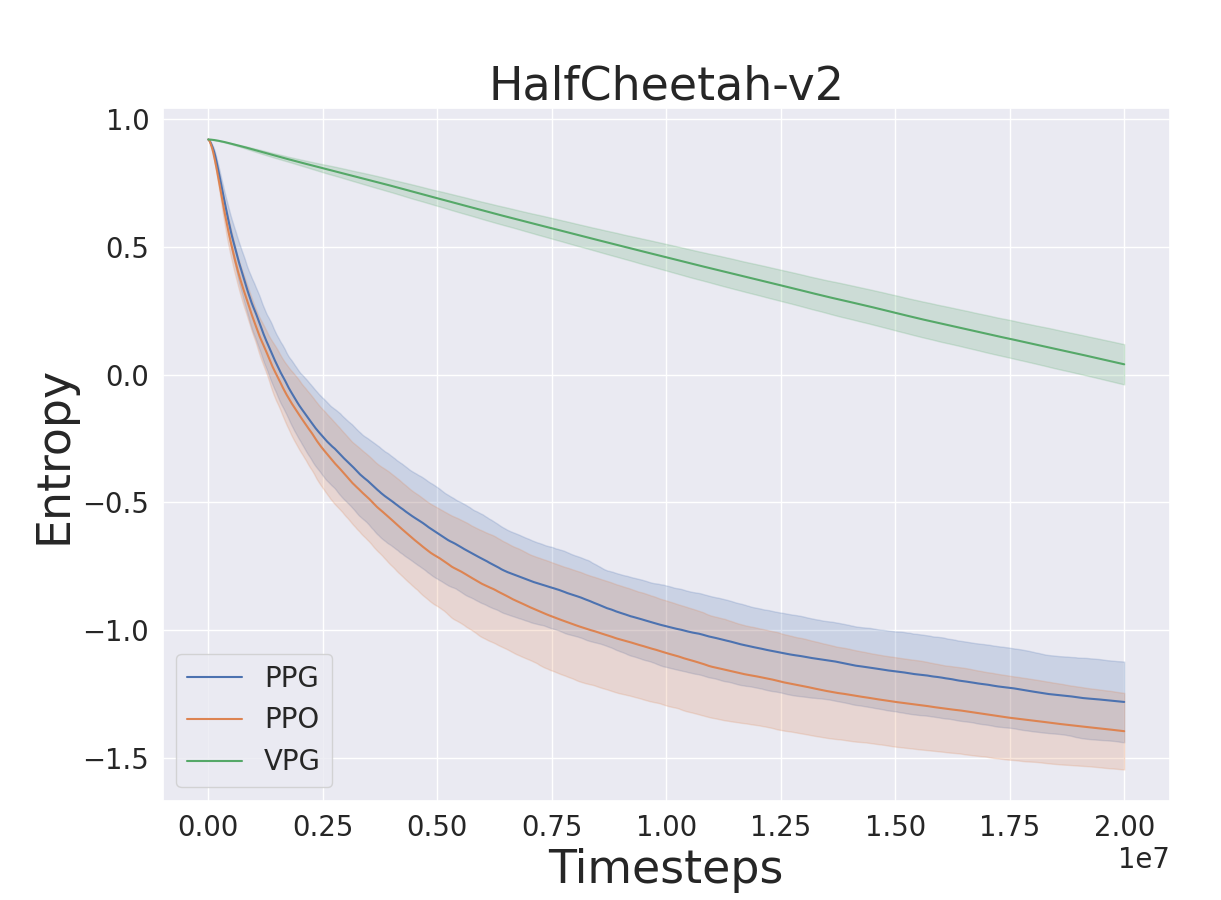
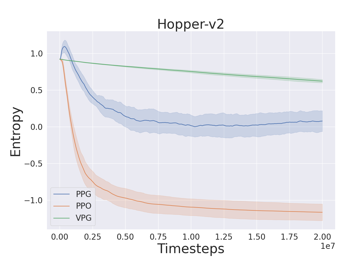
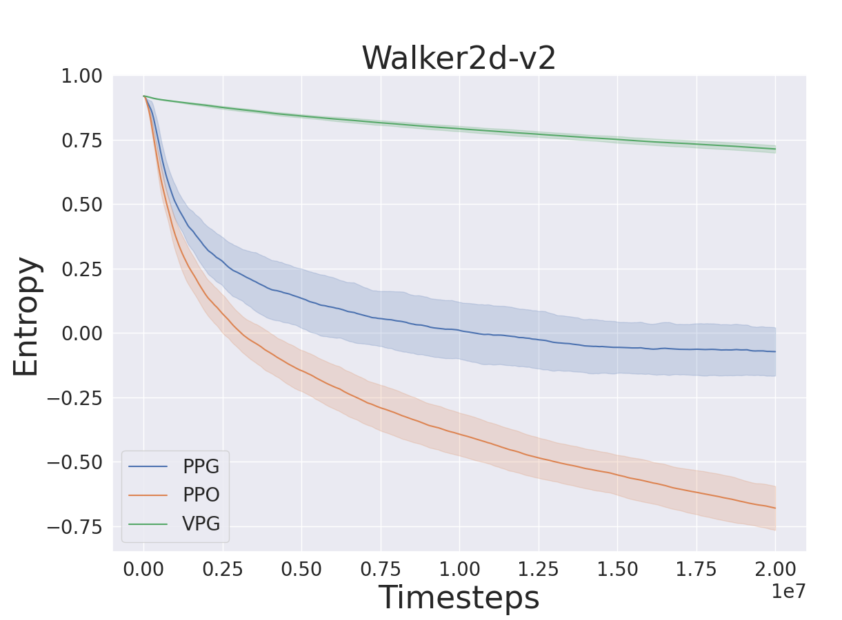
Figure 5: Average return (top) and differential entropy (bottom) from 20M interactions with the four OpenAI Gym environments with the MuJoCo physics engine. PPG and PPO perform similarly. PPG tends to produce more stochastic solutions.

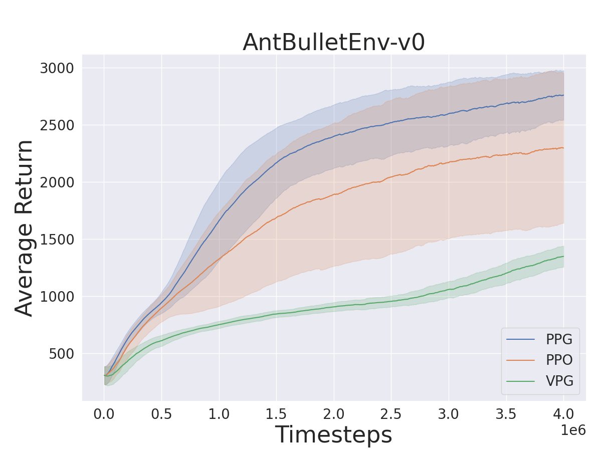
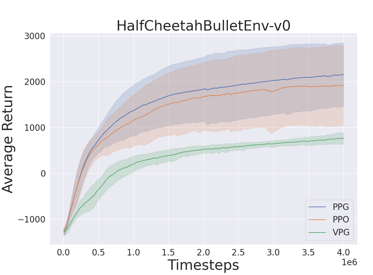
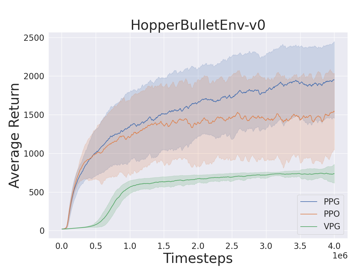
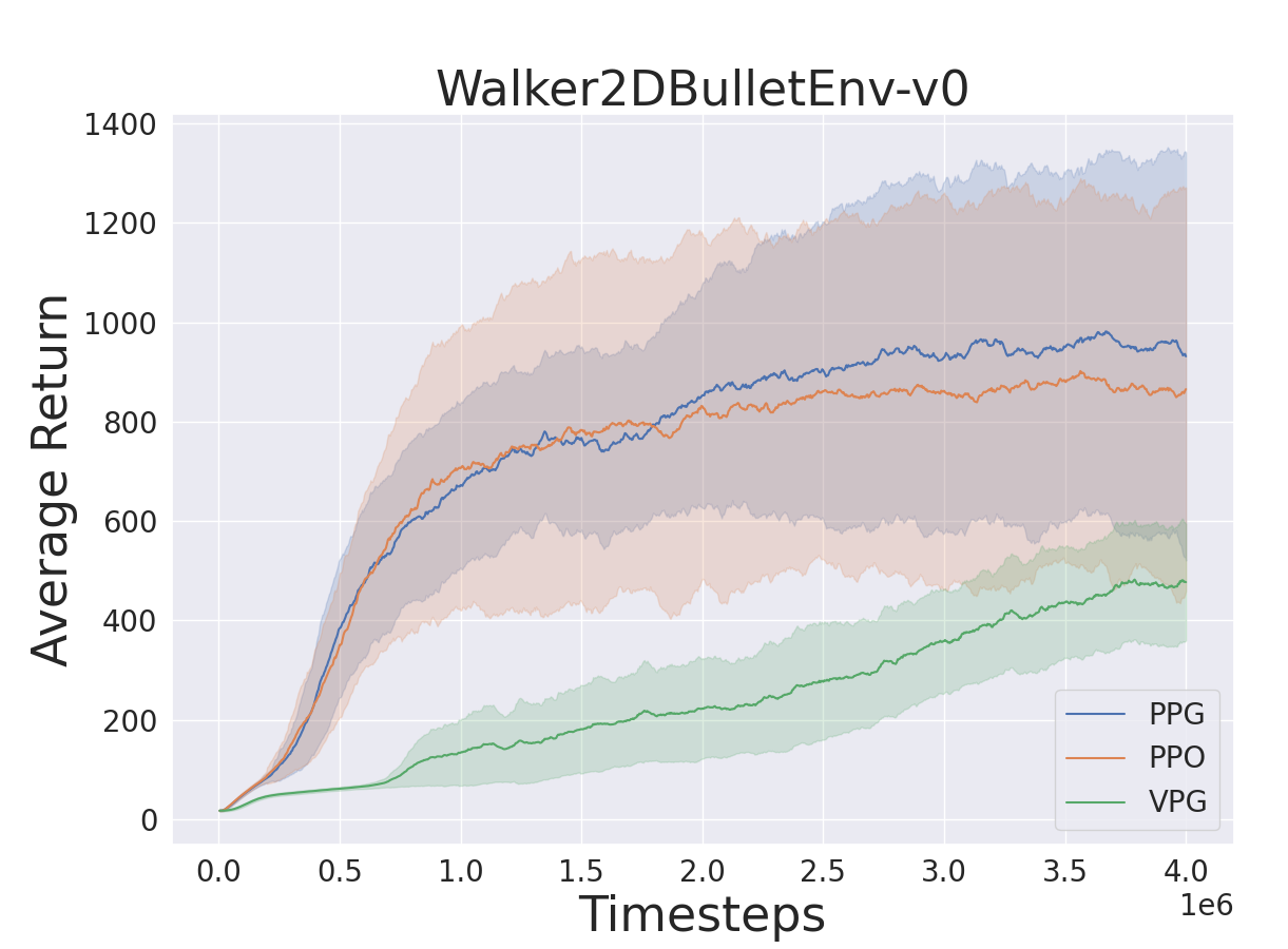
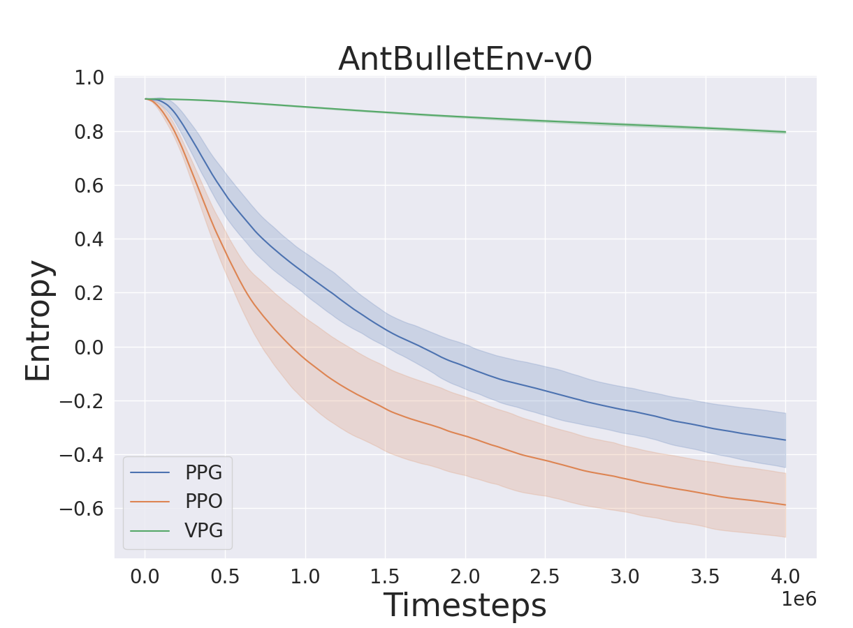
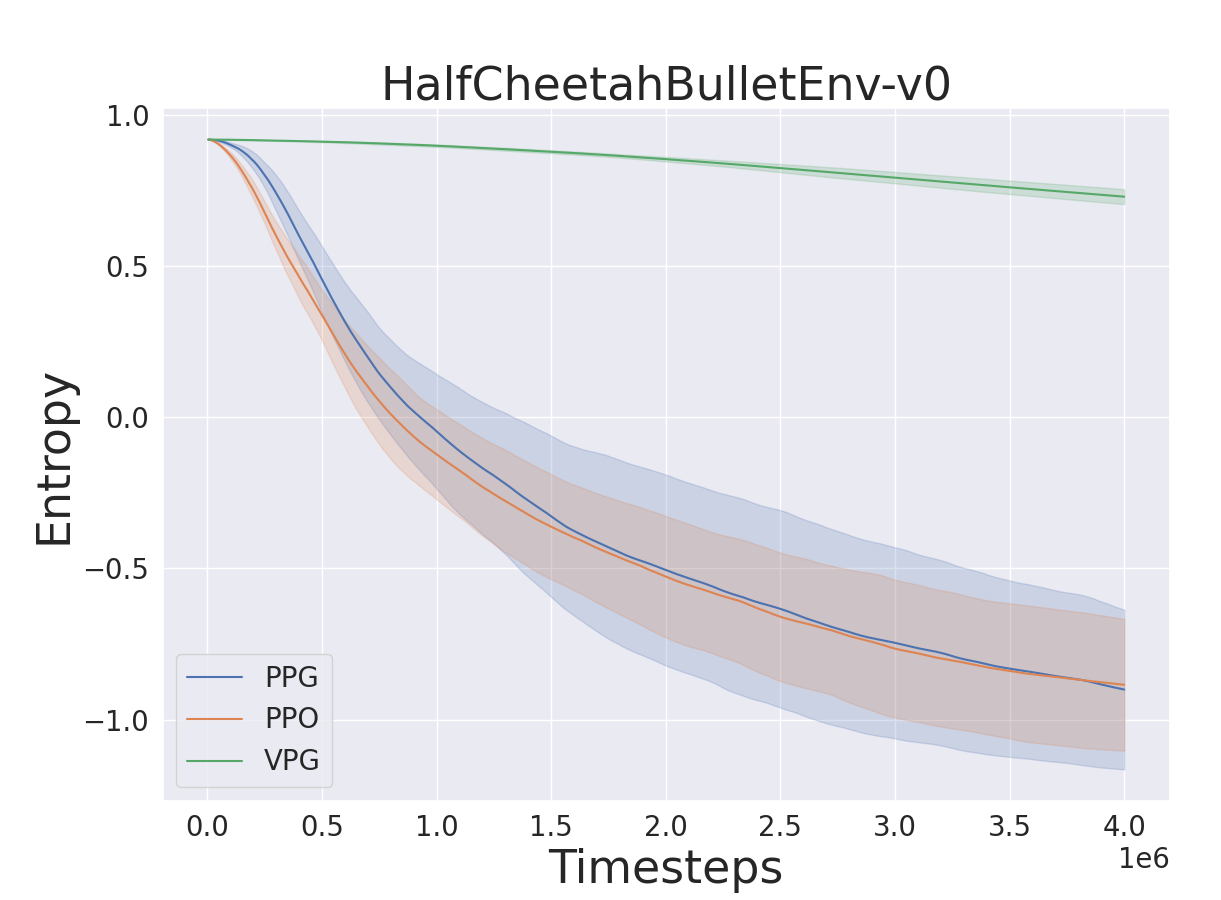
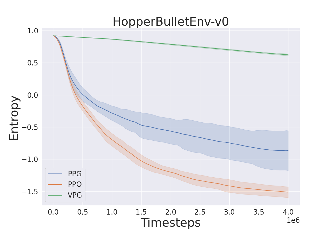
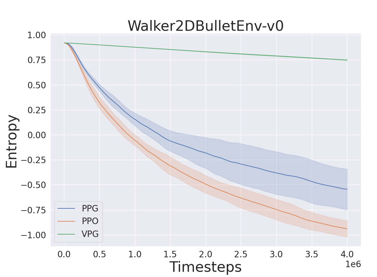
Figure 6: Average return (top) and differential entropy (bottom) from 4M interactions with the four Bullet environments. PPG and PPO perform similarly. PPG tends to produce more stochastic solutions.

Discussions on KL Divergence

As a policy update iteration continues, $\pi_{\theta}$ becomes different from $\pi_{\theta_{old}}$ as demonstrated in Fig. 1. The KL divergence, or relative entropy, measures the difference between $\pi_{\theta}$ and $\pi_{\theta_{old}}$ as

$$D_{KL}(\pi_{\theta}||\pi_{\theta_{old}})=\int\pi_{\theta}(a|s)\log\frac{\pi_{\theta}(a|s)}{\pi_{\theta_{old}}(a|s)}da$$ (6)

$D_{KL}$ can be approximated by the following $D_{MC}$, i.e., $D_{KL}\to D_{MC}$ as $n\to\infty$ (Hershey and Olsen 2007).

$$\begin{split}D_{MC}(\pi_{\theta}||\pi_{\theta_{old}})&=\frac{1}{\hat{N}}\sum_{i,t=1}^{N,T_{i}}\left(\log\pi_{\theta}(a|s)-\log\pi_{\theta_{old}}(a|s)\right)\\ &=\frac{1}{\hat{N}}\sum_{i,t=1}^{N,T_{i}}d_{i,t}\end{split}$$

Therefore, the average $y$ coordinates of all samples in the advantage-policy plane is just the approximated KL divergence $D_{MC}$. The objective $L^{\scalebox{0.55}{$PPG$}}_{\scalebox{0.55}{$NCLIP$}}=\frac{1}{\hat{N}}\sum_{i,t=1}^{N,T_{i}}d_{i,t}(\theta)\hat{A}_{t}$ has some relation to $D_{MC}$. Although $d_{i,t}(\theta)$ and $\hat{A}_{t}$ are correlated, one can easily see some trivial relations. For example, $L^{\scalebox{0.55}{$PPG$}}_{\scalebox{0.55}{$NCLIP$}}\leq\max(\hat{A}_{t})D_{MC}$ in the right half plane where $\hat{A}_{t}>0$. Since $\hat{A}_{t}$ is normalized to have the standard deviation of 1, $\max(\hat{A}_{t})$ is not large, typically less than 10.

When the iteration starts, all samples are on the x-axis. As the current policy is updated, the samples gradually spread over to all quadrants, while moving to the first and third quadrants are encouraged by the gradient. In the left half plane, since samples are driven to have decreased probabilities by the optimization, the contribution to the approximate KL divergence, $\sum_{\hat{A}_{t}<0}d_{i,t}$ is likely to be negative. In the right half plane, $\sum_{\hat{A}_{t}<0}d_{i,t}$ is likely to be positive. Since the policy network outputs log probabilities, the log probability changes in both of the half planes are often similar in magnitude. Therefore, the two KL contributions tend to cancel, yielding a small approximate KL divergence as shown in Fig. 3.

Finally, we note that we have performed preliminary tests using a number of $D_{KL}$ constraint ideas such as $D_{KL}$ penalty added to the loss $L^{\scalebox{0.55}{$PPG$}}$ with or without various dead zones designs, for example, penalize only if $d_{i,t}>c$, where $c$ is a small constant. We also penalized using the average of exact KL divergence at each sample. In general, we found $D_{KL}$ is easy to control in PPG iterations, and the results were often positive, yet a principle that guides the choice among these methods and a study on general applicability on various environments need more thorough investigations, and hence, are left as future works.

Experiments

Algorithms and Settings

We presents Alg. 1 based on (Achiam 2018; Dhariwal et al. 2017). The policy $\pi_{\theta}$ and the value network $V_{\phi}$, parameterized by $\phi$, are the fully connected networks with two layers of size 64. We used hyperbolic tangent activation functions for all layers. For each epoch, after extracting trajectory samples, $A_{t}^{GAE}$ is computed and normalized. For VPG, the policy iteration is done once, and for PPG and PPO, the iteration is continued up to 80.

PPG and PPO perform the clipping step to update the policy within the trust region. This clipping functions have the clip range (5), (4) (In our experiments, $u_{b}=0.2,\;l_{b}=-0.2,\;\epsilon=0.2$). The lines 9 to 11 in Alg. 1 implement a secondary optimization technique: if the approximated KL divergence reaches to the target $D_{MC}^{Target}$, which we choose 0.015, the policy update iteration is halted. Without this policy learning became unstable in most of the environments. After the policy iteration, $V_{\phi}$ is updated by minimizing the mean square error $||\hat{R}_{t}-V_{\phi}||^{2}$.

Algorithm 1 VPG, PPO, PPG

1:  Input: an initialized policy $\pi_{\theta}$ and value function $V_{\phi}$

2:  for $k=1$ to epoch

3:     Set $\pi_{\theta_{old}}\leftarrow\pi_{\theta}$

4:     Collect trajectories $\{\tau_{1},\tau_{2},\tau_{3},...\}$ from $\pi_{\theta_{old}}$

5:     Compute return $\hat{R}_{t}$

6:     Compute each $A_{t}^{GAE}$ using $V_{\phi}$

7:     for $i=1$ to $n$  ($n$=1 when VPG)

8:        Compute loss (2), (4), or (5)

9:        $m_{KL}\leftarrow$ the mean of the approximated $D_{MC}$

10:        if $m_{KL}>D_{MC}^{Target}$ and not VPG

11:              break

12:        end if

13:        Update $\pi_{\theta}$ by maximizing loss (2), (4), or (5)

14:     end for

15:     Update $V_{\phi}$ by minimizing $||\hat{R}_{t}-V_{\phi}||^{2}$

16:  end for

Evaluation on Benchmark Tasks

We evaluated PPG on the OpenAI Gym robotics tasks (Brockman et al. 2016), and the corresponding the Bullet tasks (Ant-v2, HalfCheetah-v2, Hopper-v2, Walker2d-v2, AntBulletEnv-v0, HalfCheetahBulletEnv-v0, HopperBulletEnv-v0, Walker2DBulletEnv-v0). For each environment, we trained 10 models using ten seeds (10000,10001,10002,…,10009). In the OpenAI Gym tasks, the models are trained for 20 million interactions with the each environments, and 4 million interactions for Bullet tasks. Training results are shown in Fig. 5, 6, and trained model evaluations are provided in Table. 1. For this evaluation, we simulated 100 episodes for each model to measure the performance. We can observe that the entropy decays slower in PPG, while the average return is similar to PPO. In addition, in Fig. 3, PPG has smaller the KL divergence than PPO, under the exactly same condition in Alg. 1.

Conclusions

We have shown that the surrogate objective can be replaced by a partial variation of the original policy gradient objective that has exactly the same gradient with the original policy gradient theorem based algorithm, VPG. Similar to PPO’s clipping mechanism that updates a policy within the trust region, PPG formulates the clipping in the log space. PPG shows the average returns comparable to PPO, the often higher entropy than PPO, and the smaller KL divergence changes than PPO.

Table 1: Trained model evaluations. Each entry has ten different trained models for 10 seeds. The average rewards are computed from 1000 episodes (100 episodes for each of 10 seeds). The entropy is the average of 10 models.

OpenAI Gym (-v2)
(Reward)	PPG	PPO	VPG
Ant	5527$\pm$947.5	5583$\pm$652.8	2360$\pm$900.6
HalfCheetah	4783$\pm$1708	4310$\pm$1537	3463$\pm$1480
Hopper	1865$\pm$769.7	2292$\pm$970.2	1756$\pm$871.9
Walker2d	3943$\pm$1400	3957$\pm$1330	3209$\pm$1307
(Entropy)	PPG	PPO	VPG
Ant	-1.08$\pm$0.04	-1.27$\pm$0.02	0.02$\pm$0.01
HalfCheetah	-1.28$\pm$0.15	-1.39$\pm$0.14	0.03$\pm$0.07
Hopper	0.07$\pm$0.14	-1.16$\pm$0.11	0.61$\pm$0.02
Walker2d	-0.07$\pm$0.09	-0.68$\pm$0.08	0.71$\pm$0.01
Bullet (BulletEnv-v0)
(Reward)	PPG	PPO	VPG
Ant	2763$\pm$300.8	2322$\pm$680.1	1363$\pm$146.6
HalfCheetah	2148$\pm$729.0	1887$\pm$958.6	768$\pm$187.2
Hopper	1850$\pm$780.0	1639$\pm$654.7	728$\pm$227.8
Walker2d	958$\pm$522.2	873$\pm$515.8	482$\pm$292.9
(Entropy)	PPG	PPO	VPG
Ant	-0.35$\pm$0.10	-0.59$\pm$0.11	0.79$\pm$0.01
HalfCheetah	-0.91$\pm$0.25	-0.89$\pm$0.21	0.72$\pm$0.02
Hopper	-0.87$\pm$0.31	-1.51$\pm$0.08	0.61$\pm$0.01
Walker2d	-0.55$\pm$0.20	-0.94$\pm$0.07	0.74$\pm$0.01

References

- Achiam (2018) Achiam, J. 2018. Spinning Up in Deep Reinforcement Learning .
- Ahmed et al. (2019) Ahmed, Z.; Le Roux, N.; Norouzi, M.; and Schuurmans, D. 2019. Understanding the impact of entropy on policy optimization. 151–160.
- Andrychowicz et al. (2018) Andrychowicz, M.; Wolski, F.; Ray, A.; Schneider, J.; Fong, R.; Welinder, P.; McGrew, B.; Tobin, J.; Abbeel, P.; and Zaremba, W. 2018. Hindsight Experience Replay. arXiv preprint arXiv:1707.01495 .
- Brockman et al. (2016) Brockman, G.; Cheung, V.; Pettersson, L.; Schneider, J.; Schulman, J.; Tang, J.; and Zaremba, W. 2016. OpenAI Gym. CoRR . URL http://arxiv.org/abs/1606.01540.
- Dhariwal et al. (2017) Dhariwal, P.; Hesse, C.; Klimov, O.; Nichol, A.; Plappert, M.; Radford, A.; Schulman, J.; Sidor, S.; Wu, Y.; and Zhokhov, P. 2017. OpenAI Baselines. https://github.com/openai/baselines.
- Engstrom et al. (2020) Engstrom, L.; Ilyas, A.; Santurkar, S.; Tsipras, D.; Janoos, F.; Rudolph, L.; and Madry, A. 2020. Implementation Matters in Deep RL: A Case Study on PPO and TRPO. URL https://openreview.net/forum?id=r1etN1rtPB.
- Fujimoto et al. (2018) Fujimoto, S.; van Hoof, H.; ; and Meger, D. 2018. Addressing function approximation error in actor-critic methods. arXiv preprint arXiv:1802.09477, 2018 .
- Haarnoja et al. (2018) Haarnoja, T.; Zhou, A.; Abbeel, P.; and Levine, S. 2018. Soft actor-critic: Off-policy maximum entropy deep reinforcement learning with a stochastic actor. arXiv preprint arXiv:1801.01290 .
- Hershey and Olsen (2007) Hershey, J. R.; and Olsen, P. A. 2007. Approximating the Kullback Leibler divergence between Gaussian mixture models. IV–317. IEEE.
- Lillicrap et al. (2015) Lillicrap, T. P.; Hunt, J. J.; Pritzel, A.; Heess, N.; Erez, T.; Tassa, Y.; Silver, D.; and Wierstra, D. 2015. Continuous control with deep reinforcement learning. arXiv preprint arXiv:1509.02971 .
- Liu et al. (2019) Liu, Z.; Li, X.; Kang, B.; and Darrell, T. 2019. Regularization matters in policy optimization. arXiv preprint arXiv:1910.09191 .
- Mnih et al. (2016) Mnih, V.; Badia, A. P.; Mirza, M.; Graves, A.; Lillicrap, T.; Harley, T.; Silver, D.; and Kavukcuoglu, K. 2016. Asynchronous methods for deep reinforcement learning. 1928–1937.
- Mnih et al. (2015) Mnih, V.; Kavukcuoglu, K.; Silver, D.; Rusu, A. A.; Veness, J.; Bellemare, M. G.; Graves, A.; Riedmiller, M.; Fidjeland, A. K.; Ostrovski, G.; Petersen, S.; Beattie, C.; Sadik, A.; Antonoglou, I.; King, H.; Kumaran, D.; Wierstra, D.; Legg, S.; and Hassabis, D. 2015. Human-level control through deep reinforcement learning. Nature (7540): 529–533. ISSN 00280836. URL http://dx.doi.org/10.1038/nature14236.
- Schulman et al. (2015a) Schulman, J.; Levine, S.; Abbeel, P.; Jordan, M.; and Moritz, P. 2015a. Trust Region Policy Optimization. 1889–1897. Lille, France: PMLR. URL http://proceedings.mlr.press/v37/schulman15.html.
- Schulman et al. (2015b) Schulman, J.; Moritz, P.; Levine, S.; Jordan, M.; and Abbeel, P. 2015b. High-dimensional continuous control using generalized advantage estimation. arXiv preprint arXiv:1506.02438 .
- Schulman et al. (2017) Schulman, J.; Wolski, F.; Dhariwal, P.; Radford, A.; and Klimov, O. 2017. Proximal Policy Optimization Algorithms. CoRR . URL http://arxiv.org/abs/1707.06347.
- Sutton and Barto (2018) Sutton, R. S.; and Barto, A. G. 2018. Cambridge, MA, USA: MIT Press. ISBN 978-0262039246.
- Sutton et al. (1999) Sutton, R. S.; McAllester, D.; Singh, S.; and Mansour, Y. 1999. Policy gradient methods for reinforcement learning with function approximation: actor-critic algorithms with value function approximation. 1057–1063.
- Sutton et al. (2000a) Sutton, R. S.; McAllester, D. A.; Singh, S. P.; and Mansour, Y. 2000a. Policy Gradient Methods for Reinforcement Learning with Function Approximation. 1057–1063. MIT Press. URL http://papers.nips.cc/paper/1713-policy-gradient-methods-for-reinforcement-learning-with-function-approximation.pdf.
- Sutton et al. (2000b) Sutton, R. S.; McAllester, D. A.; Singh, S. P.; and Mansour, Y. 2000b. Policy gradient methods for reinforcement learning with function approximation. 1057–1063.
- Wang et al. (2019) Wang, Y.; He, H.; Tan, X.; and Gan, Y. 2019. Trust region-guided proximal policy optimization. 626–636.
- Watkins (1989) Watkins, C. J. C. H. 1989. Learning from delayed rewards .
- Williams (1992) Williams, R. J. 1992. Simple statistical gradient-following algorithms for connectionist reinforcement learning. Machine learning (3-4): 229–256.
- Zhang, Wu, and Pineau (2018) Zhang, A.; Wu, Y.; and Pineau, J. 2018. Natural environment benchmarks for reinforcement learning. arXiv preprint arXiv:1811.06032 .