Hierarchical Paired Channel Fusion Network for Street Scene Change Detection

Abstract

Street Scene Change Detection (SSCD) aims to locate the changed regions between a given street-view image pair captured at different times, which is an important yet challenging task in the computer vision community. The intuitive way to solve the SSCD task is to fuse the extracted image feature pairs, and then directly measure the dissimilarity parts for producing a change map. Therefore, the key for the SSCD task is to design an effective feature fusion method that can improve the accuracy of the corresponding change maps. To this end, we present a novel Hierarchical Paired Channel Fusion Network (HPCFNet), which utilizes the adaptive fusion of paired feature channels. Specifically, the features of a given image pair are jointly extracted by a Siamese Convolutional Neural Network (SCNN) and hierarchically combined by exploring the fusion of channel pairs at multiple feature levels. In addition, based on the observation that the distribution of scene changes is diverse, we further propose a Multi-Part Feature Learning (MPFL) strategy to detect diverse changes. Based on the MPFL strategy, our framework achieves a novel approach to adapt to the scale and location diversities of the scene change regions. Extensive experiments on three public datasets (i.e., PCD, VL-CMU-CD and CDnet2014) demonstrate that the proposed framework achieves superior performance which outperforms other state-of-the-art methods with a considerable margin.

I Introduction

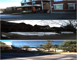
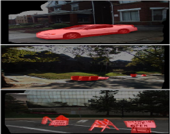
(a) Image at $t_{0}$	(b) Image at $t_{1}$	(c) Change map

Figure 1: Examples of the SSCD task. (a) The image at time $t_{0}$; (b) The image at time $t_{1}$; (c) The predicted change map which are highlighted in red.

Scene Change Detection (SCD) aims to find the changed regions between a pair of images captured at different times. This task has been attracting growing research interest as its various real-world applications, e.g., global resources monitoring, land-use change detecting, disaster evaluation, visual surveillance and urban management. In recent years, two SCD application scenarios have seen a lot of research activities, i.e., Remote Sensing and Street Surveillance. Many researchers [1, 2, 3, 4, 5, 6] have made efforts on the topic of Remote-Sensing SCD (RSSCD) for the purpose of information analysis on earth’s surface. Meanwhile, important contributions [7, 8, 9, 10, 11] have been devoted to Street Scene Change Detection (SSCD) aiming to overcome the issues of urban management. In this paper, we focus on SSCD. A sample illustration of the SSCD task is shown in Fig. 1. The fundamental method for the SSCD task is to combine the extracted features from the input image pair, and then the SSCD is cast as a pixel-wise classification task for generating a change map. Intuitively, the information fusion from different sources plays an important role in the SSCD task since the change map is jointly determined by the input image pair. During the past decades, lots of SSCD methods have been proposed [12, 13, 14, 15, 16, 17, 3]. Most of these methods adopt handcrafted features as detection cues. However, the handcrafted features suffer from some inherent drawbacks, e.g., low robustness and insufficient semantics, which significantly hinder the performance of the SSCD task. Recently, deep Convolutional Neural Networks (CNNs) [18, 19, 20] have been successfully applied to various pixel-wise image classification tasks due to their great capabilities to extract multi-level feature representations. Encouraged by their strengths, researchers [7, 21, 10, 11, 8, 9] start to leverage CNNs to automatically fuse features from different sources for the SSCD task in order to avoid the intrinsic drawbacks of handcrafted features.

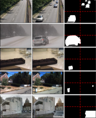
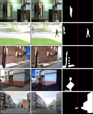
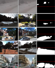
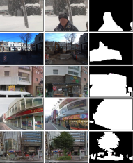
(a) Corner	(b) Left and right	(c) Top and bottom	(d) Center

Figure 2: Examples from three widely-used datasets: PCD, VL-CMU-CD and CDnet2014. We can see that the locations and scales of changed regions are unbalanced in the dataset. It can be divided into four cases: (a) corner, (b) left and right, (c) top and bottom and (d) center.

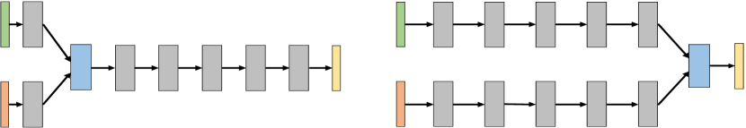
(a) Single-level feature fusion: Early Fusion (left) and Late Fusion (right).

(b) Multi-level feature fusion: Dense Fusion.

Figure 3: Existing fusion structures for the SSCD task. (a) Early Fusion and Late Fusion are adopted in single-level fusion. (b) Dense Fusion is adopted in multi-level fusion.

As shown in Fig. 3, the CNN based SSCD methods can be coarsely classified into two groups: single-level feature fusion methods, and multi-level feature fusion methods. In the past few years, many methods [7, 21, 10, 9, 11] adopt single-level feature based architecture, e.g., early-fusion or late-fusion (Fig. 3 (a)), which fuse the features from different sources at a specific fusion position.

However, the single-level feature methods can only fuse partial information for the SSCD task, which may hinder the detection performance. In contrast, the multi-level feature methods are capable of representing different characteristics of change scenes, which can significantly improve the performance. Therefore, several multi-level feature based methods have been proposed [8, 22], which perform the dense feature fusion (shown in Fig. 3 (b)) in a deep-to-shallow manner. However, most of existing multi-level feature fusion methods follow a simple fusion manner, i.e., concatenation or summation operation. As many visualization works shown, the features at shallow layers of deep networks contain low-level vision information, such as image texture, object boundary, scene edge, etc. With the increase of layers, the hierarchical features will become more abstractive. In general, the deep layers have high-level information, such as image content, semantic concept, etc. Thus, there are semantic gaps at different levels of network layers. Such a naive fusion ignores the semantic relationship between different feature maps.

To address the above problems, we propose a novel Hierarchical Paired Channel Fusion Network (HPCFNet), which is a more effective framework for the multi-level feature fusion. Specifically, for each feature level, we introduce a Paired Channel Fusion (PCF) module which enables the cross-image feature fusion to sufficiently capture the channel-wise changes. The paired image features are jointly extracted by a Siamese Convolutional Neural Network (SCNN), and then hierarchically combined in a coarse-to-fine manner. In addition, a Reverse Spatial Attention (RSA) mechanism is presented to highlight the changed regions while suppressing the unchanged regions.

Besides, we observe that both the locations and scales of changed regions are diverse in the dataset. As shown in Fig. 2, the spatial distribution of changed regions is diverse and changed regions contain various scales. For example, the changed regions in Fig. 2 (a) are located in the corner and have small scales, while those in Fig. 2 (d) are located in the center with large scales. The imbalance can be divide into 4 cases: (a) corner, (b) left and right, (c) top and bottom and (d) center. Based on the above observations, we propose a Multi-Part Feature Learning (MPFL) strategy, which adapts to the location and scale variations. More specifically, the MPFL strategy consists of four branches with different partition methods. Four branches utilize adaptive convolutional layers to capture the discriminative characteristics from different spatial parts. The proposed framework has been evaluated on three large-scale SSCD datasets, i.e., PCD [11], VL-CMU-CD [21] and CDnet2014 [23]. Experimental results have demonstrated that the proposed framework outperforms other state-of-the-art methods with a considerable margin.

Our contributions can be summarized as follows:

• We propose a novel framework, named HPCFNet for the challenging SSCD task. The HPCFNet efficiently utilizes a dense fusion architecture for multi-level feature fusion. Besides, an effective RSA module is incorporated to highlight changed regions from the fused feature maps.

• We propose a novel MPFL strategy to detect changed regions from holistic to local. The MPFL addresses the spatial distribution and diverse scales of changed regions by using four different partition methods.

• Comprehensive experiments on three public SSCD datasets demonstrate that the proposed framework achieves superior performance and outperforms other state-of-the-art methods with a considerable margin.

The reminder of this work is organized as follows. Section II presents an overview of related works on change detection, feature fusion and attention mechanism. Section III describes our proposed method in detail. The experimental setups and results are provided in Section IV and Section V, respectively. The conclusions are drawn in Section VI.

II Related Works

II-A Change Detection

In the past few years, with the development of semantic segmentation [18, 24, 22, 25, 26, 27, 28], many SSCD methods have been proposed. The technical comparisons of different handcrafted feature based methods are summarized in [29]. A detailed review is beyond the scope of this work. In this section, we mainly describe SSCD methods based on deep learning.

In recent years, deep neural networks have been successfully applied in many research fields and have achieved the most advanced performance. Almost all the excellent SSCD methods are based on pre-trained CNN backbones [30, 20, 31, 32, 33, 34, 35], and many of them are based on Fully Convolutional Networks (FCN) [18]. For example, Sakurada et al. [11] calculated the distance between features extracted from paired CNNs, and eliminated the geometric background context by superpixel segmentation. Guo et al. [9] proposed to learn the distinguishing features with the customized feature distance metrics. Zhan et al. [36] proposed a contrastive loss function for CNNs, which increases the distance of the feature points which are identified as changed and reduces the distance of the feature points which are identified as unchanged. Sakurada et al. [7] utilized dense optical flow and CNNs to model the spatial correspondences between images captured at different times. Alcantarilla et al. [21] used the dense geometry and accurate registration to warp images from different times for the change comparison. Khan et al. [10] proposed a deep CNN with Directed Acyclic Graph (DAG) topologies to measure image changes. Sakurada et al. [8] introduced hierarchically dense connections to capture the multi-scale feature information.

Although previous methods achieve remarkable performance for the SSCD task, they still have several unsolved problems. Most of the recent deep learning methods focus on adding auxiliary information, designing loss functions or using additional data. However, few of them have focused on further improvement of feature fusion, especially fusion based on multi-level features. To solve this problem, we introduce a novel feature fusion network to hierarchically exploit paired channel differences of multi-level features.

II-B Feature Fusion

Encouraged by the remarkable strengths of deep CNNs, a few methods for the SSCD task leverage CNNs to fuse information from different image sources. In [21, 10, 7], the information from two sources was combined at a shallow position. In contrast, late fusion based methods [9, 11] fuse the two source features at a deep position. Essentially, the early fusion and late fusion can be merged as a single-level feature fusion strategy. Though the single-level feature fusion strategy achieves encouraging performance, it does not utilize all the available information. Due to the powerful ability of presentations, the features at other levels are also important for the SSCD task.

To take advantage of multi-level features, the method in [8] has been introduced by using dense fusion positions inside the networks[25, 27, 37, 26, 24]. However, this method still follows the traditional fusion manner such as concatenation and element-wise addition to combine multiple features. In order to address this problem, we propose a novel Paired Channel Fusion (PCF) module to sufficiently fuse the channel pairs at each feature level. In the PCF module, we utilize atrous convolutions with various dilation rates to generate diverse fused features.

II-C Attention Mechanism

Attention mechanisms have been developed over many decades in neuroscience community [38, 39, 40, 41] and have played a vital role in current deep neural networks [42, 43]. Previous works in [43, 44, 41, 45, 46] have shown the importance of attention mechanism, which uses high-level information to weigh features at the middle of networks. Attention usually cooperates with gating functions (e.g., softmax and sigmoid function), and has achieved excellent performance for sequence and image localization [47, 44]. Recently, Hu et al. [48] proposed a self-attention unit called the Squeeze-and-Excitation (SE) block. The goal of the SE block is to ensure that the network can highlight related features and suppress the less useful features. Woo et al. [49] proposed the Convolutional Block Attention Module (CBAM) to intensify the meaningful information on both channel and spatial axis. Channel and spatial attention modules are jointly utilized to learn task-related features of multiple branches. Inspired by previous works, we propose a Reverse Spatial Attention (RSA) module to generate an attention mask by pooling operations (average pooling and max pooling) and feature reversing. The RSA highlights the changed regions based on the fused feature maps of two extracted feature maps.

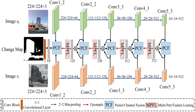
Figure 4: The overall architecture of the HPCFNet. “A” denotes the Reverse Spatial Attention (RSA) module. Paired Channel Fusion (PCF) modules are used for channel-wise feature fusion. The Multi-Part Feature Learning (MPFL) integrates the features from holistic to local scales, and adapt to various change distributions.

(a) Images at $t_{0}$ and $t_{1}$

(b) Feature maps at the same channel

Figure 5: Typical examples of paired feature maps. (a) Input images at different times. (b) Paired feature maps at the 12-th channel, which are extracted from the Conv4_3 layer of the SCNN. We resize and overlay them on original images for better visualization.

TABLE I: The detailed configurations of our HPCFNet. In each row, the numbers denote the corresponding channel number of the output feature map. C, L, and B denote the layer of 3$\times 3$ convolution, Leaky ReLU and batch normalization.

Location	PCF	RSA	Conv Block	MPFL
Conv1_2	192	-	CLB, 64	-
Conv2_2	384	384	CLB, 128	64
Conv3_3	768	768	CLB, 256	128
Conv4_3	1280	1280	CLB, 512	256
Conv5_3	1024	1024	CLB, 512	256

III Methodology

III-A Overall Architecture

The overall architecture of the proposed HPCFNet is shown in Fig. 4. For the SSCD task, the main steps can be briefly described as follows. First, the paired images at different times ($t_{0}$ and $t_{1}$) are fed into a Siamese Convolutional Neural Network (SCNN) with the VGG-16 backbone [33] to extract multi-level deep features. Then, feature maps from convolutional layers (i.e., conv1_2, conv2_2, conv3_3, conv4_3 and conv5_3) are integrated by the proposed PCF modules to generate channel-wise fused feature maps, hierarchically. Afterwards, the fused feature maps are adjusted by the RSA modules. The MPFL strategy is inserted to detect changes in a holistic-to-local manner. Finally, the change map is predicted by combining the hierarchical fused features. Tab. I shows the detailed configurations of the proposed HPCFNet.

III-B Paired Channel Fusion

To fuse feature maps, the most straightforward method is to concatenate them in channel-wise. However, as a result, the characteristics of the fused feature maps can’t be well explored. Therefore, it is cumbersome to detect change regions. By visualizing the channels of the SCNN (shown in Fig. 5), we observe that the paired channels from the same layer in the two streams, can activate most of the changed regions.

Figure 6: An illustration of the proposed PCF module. $F_{t_{0}}^{m}$ and $F_{t_{1}}^{m}$ are the $m$-th level feature maps extracted from images at $t_{0}$ and $t_{1}$, respectively.

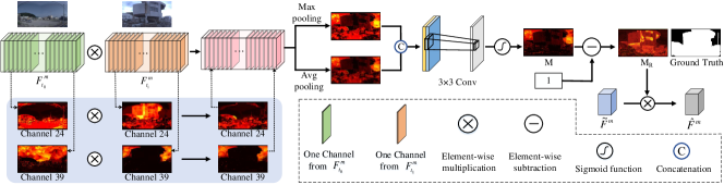
Figure 7: The detailed architecture of the RSA module. In order to show the operation clearly, we here illustrate the changing process of channel features for a definite input image pair.

Thus, paired channels extracted at the same level can contribute to locating the changed regions. Inspired by this fact, we propose an effective fusion method named Paired Channel Fusion (PCF) to incorporate the information of paired channels. The overall architecture of the PCF is shown in Fig. 6. More specifically, at the $m$-th level, we first combine the same-level feature maps (i.e., $\textbf{F}_{t_{0}}^{m}$ and $\textbf{F}_{t_{1}}^{m}$) by the Cross Feature Stack (CFS) to make the channels interweave, resulting in $\textbf{F}_{s}^{m}$. Motivated by Atrous Spatial Pyramid Pooling (ASPP) module [50], we propose a Parallel Atrous Group Convolution (PAGC) module to fuse paired channels and capture multi-scale feature representations. The PAGC module has four separate group convolutions with kernel size of $3\times 3$. For simplicity, the group number of each group convolutional layer is set to $c$, which is the channel number of the input $\textbf{F}_{t_{0}}^{m}$ or $\textbf{F}_{t_{1}}^{m}$. Thus, each group in the group convolutional layer contains two channels: one channel from $\textbf{F}_{t_{0}}^{m}$, and the corresponding channel from $\textbf{F}_{t_{1}}^{m}$. In addition, we use dilated convolution to enlarge the receptive fields. The outputs of four group convolutions are concatenated, then reduced through a $1\times 1$ convolutional layer to avoid too much computation. The output of a PAGC (i.e., $\bar{\textbf{F}}^{m}$) is concatenated with the processed feature map from the $(m+1)$-th level (i.e., $\textbf{F}^{m+1}$) to produce the output of the PCF module (i.e., $\widetilde{\textbf{F}}^{m}$).

The PCF can be formulated as:

$$\small\bar{\textbf{F}}^{m}=g^{1\times 1}([f_{d=1}^{3\times 3}(\textbf{F}_{s}^{m}),f_{d=2}^{3\times 3}(\textbf{F}_{s}^{m}),f_{d=3}^{3\times 3}(\textbf{F}_{s}^{m}),f_{d=4}^{3\times 3}(\textbf{F}_{s}^{m})]),$$ (1)

$$\small\widetilde{\textbf{F}}^{m}=[\bar{\textbf{F}}^{m},\textbf{F}^{m+1}]$$ (2)

where $f_{d=n}^{k\times k}$ denotes the atrous group convolution which consists of (i) a convolutional layer with a group number $c$, kernel size $k\times k$ and dilation $n$, (ii) a batch normalization [51], and (iii) a non-liner activation function. $[\cdot]$ denotes the channel-wise concatenation. $g^{1\times 1}$ is a $1\times 1$ convolutional layer.

III-C Reverse Spatial Attention

The fused feature map produced by the PCF module can coarsely locate the changed regions, however, it lacks the capacity of highlighting regional details. To solve this problem, we further introduce a Reverse Spatial Attention (RSA) module, as shown in Fig. 7. We feed $\widetilde{\textbf{F}}^{m}$, $\textbf{F}_{t_{0}}^{m}$ and $\textbf{F}_{t_{1}}^{m}$ into the RSA module to produce the weighted fused feature map.

It is well known that, the Siamese network extracts features of two different images in the same way. Hence the changeless regions in paired images result in feature maps that contain the same semantic information. Meanwhile, the changed regions result in different activations on paired feature maps. In our RSA (Fig. 7), we first perform the element-wise multiplication ( $\textbf{F}_{t_{0}}^{m}$ and $\textbf{F}_{t_{1}}^{m}$) to enhance the same information. After multiplication, each two corresponding channels will keep the changed regions non-activated. This is due to changed regions will lead to large different activation values in corresponding channels. From Fig. 7, one can observe that whether in channel 24 or channel 39, the changed area is non-activated after multiplication. Due to the limitation of space, we only show the changing process of channel 24 and channel 39. The other channels have a similar trend. Therefore, after pooling along the channel axis, the changed regions are remain non-activated. Specifically, an average-pooling and a max-pooling are separately executed along the channel axis to capture the statistical properties of feature maps [49]. The resulting feature maps are concatenated and fed into a $3\times 3$ convolutional layer to generate a spatial attention mask $\textbf{M}\in R^{h\times w\times 1}$. Because the multiplied features emphasize the same representations of two feature maps. The generated M is capable of highlighting the changeless regions. However, for change detection, we prefer to highlight the changed regions. Thus, the reversed mask is more effective for the SSCD task. Formally, the mask $\textbf{M}_{R}$ can be computed by:

$$\small\textbf{M}_{R}=\textbf{1}-\sigma(\textbf{W}^{T}[AP(\textbf{F}_{t_{0}}^{m}\odot\textbf{F}_{t_{1}}^{m}),MP(\textbf{F}_{t_{0}}^{m}\odot\textbf{F}_{t_{1}}^{m})]+\textbf{b}),$$ (3)

where $\sigma$ denotes a sigmoid function. W and b denote learn-able parameters. $AP(\cdot)$ and $MP(\cdot)$ are the average-pooling and max-pooling, respectively. $\odot$ denotes the element-wise multiplication. Based on the RSA mask, the attentive features can be expressed as:

$$\small\hat{\textbf{F}}_{i,j,k}^{m}=\textbf{M}_{R}\odot\widetilde{\textbf{F}}_{i,j,k}^{m},$$ (4)

where $(i,j,k)$ denotes the width, height and channel index of the feature maps. Note that the attention mask $\textbf{M}_{R}$ is duplicated $k$ times to weight every channel.

III-D Multi-Part Feature Learning

As mentioned in Section I, both the locations and the scales of changed regions are unbalanced in the dataset. To address this problem, we propose a novel MPFL strategy which detects changes from global to local. As shown in Fig. 2, we observe that the diversity can be divided into four cases. Therefore we design four corresponding partitions for above cases, which are presented in Fig. 8. More specifically, given the attentive feature $\hat{\textbf{F}}^{m}$, a $1\times 1$ convolutional layer is first performed to reduce the channel dimension, resulting in $\check{\textbf{F}}^{m}$. Then, we partition the features as follows: ① dividing the original feature $\check{\textbf{F}}^{m}$ into 4 feature blocks (Branch 1) along the height and width where each feature block has the size of $(h/2)\times(w/2)\times c$; ② dividing the $\check{\textbf{F}}^{m}$ into $2$ feature blocks (Branch 2) only along the width axis where each feature block has the size of $h\times(w/2)\times c$; ③ dividing the $\check{\textbf{F}}^{m}$ into $2$ feature blocks (Branch 3) only along the height axis where each feature block has the size of $(h/2)\times w\times c$; ④ The final branch (Branch 4) is the original feature $\check{\textbf{F}}^{m}$. For each branch, we set specific kernel sizes to adapt to different scales of feature blocks, i.e., $1\times 1$ in Branch 1, $3\times 1$ in Branch 2, $1\times 3$ in Branch 3 and $3\times 3$ in Branch 4. Note that in each branch, the convolution of each feature block is independent. Hence MPFL can adaptively learn global and local features with appropriate receptive fields. Finally, we concatenate all the feature maps of different branches. In the proposed MPFL strategy, the four branches utilize different spatial partition approaches and adaptive convolutional layers, thus they can capture the discriminative characteristics from different spatial regions. Based on the MPFL strategy, the performance of SSCD can be significantly improved as shown in Section V. D.

III-E Network Training

Given the training dataset as $\left\{(X_{t_{0}}^{n},X_{t_{1}}^{n}),Y^{n}\right\}_{n=1}^{N}$, where $(X_{t_{0}}^{n},X_{t_{1}}^{n})$ is the paired image, $Y^{n}$ is the ground-truth change map, and $N$ is the total number of training examples. $Y_{l}^{n}$ denotes the $l$-th pixel of $Y^{n}$. Without loss of generality, we subsequently drop the superscript $n$ and consider each pixel for the network training.

The softmax cross-entropy loss function is effective for most image pairs which include large change areas. However, for a typical natural image, the class distribution of changed/non-changed pixels is heavily imbalanced. To relieve the class-imbalance problem, we adopt the weighted cross-entropy loss function to train our model. Formally, the loss function can be calculated by:

$$\mathcal{L}=-\frac{1}{L}\sum_{l=1}^{L}\sum_{j=0}^{1}w_{j}\text{log~{}Pr}(Y_{l}=j|(X_{t_{0}}^{n},X_{t_{1}}^{n});\theta),$$ (5)

where $w_{j}$ is a weight for class $j$, $\text{Pr}(Y_{l}=j|X;\theta)$ is the probability that measures how likely the pixel belongs to the $j$-th class. For the weights, we adopt:

$$w_{0}=1-\frac{n_{T}}{n_{T}+n_{F}},w_{1}=\frac{n_{T}}{n_{T}+n_{F}},$$ (6)

where $n_{T}$ denotes the number of pixels which are set in true class, and $n_{F}$ denotes that of pixels in the other class. The $n_{T}+n_{F}$ is the total number of pixels. The above loss function is continuously differentiable, so we can use the standard Stochastic Gradient Descent (SGD) method [52] to obtain the optimal parameters.

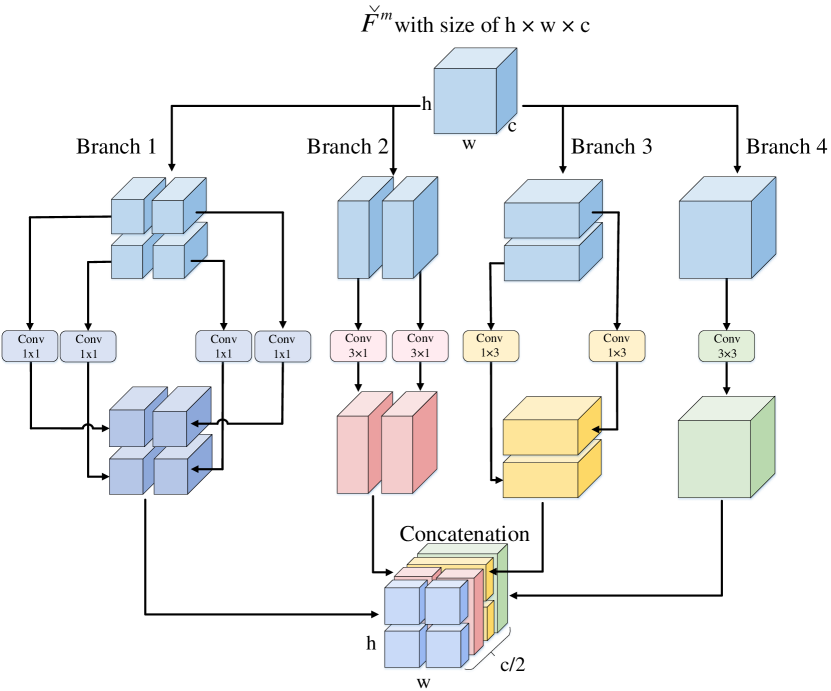
Figure 8: An illustration of the Multi-Part Feature Learning (MPFL) strategy. The feature map is fed into 4 independent branches.

IV Experimental Setups

In order to demonstrate the effectiveness of the proposed method, we evaluate it on three public benchmark datasets, i.e., PCD [11], VL-CMU-CD [21] and CDnet2014 [23]. We first introduce details of the three publicly available datasets. Then, we present the evaluation metrics and implementation details. Afterwards, we compare our results against other state-of-the-art methods. Finally, we conduct ablation experiments to demonstrate the effects of different modules.

IV-A Street Scene Change Detection Datasets

The PCD dataset [11] consists of two subsets, i.e., “GSV” and “TSUNAMI”. Each subset consists of 100 panoramic image pairs and the hand-labeled change masks. The camera viewpoints of every image pair are different. In detail, the GSV dataset consists of 100 panoramic image pairs of Google Street View, and the TSUNAMI dataset consists of 100 panoramic image pairs of scenes after a tsunami.

The VL-CMU-CD dataset [21] is a street-view change detection dataset with a long time span. It contains 151 image sequences for change detection. It can generate a total of 1362 image pairs, each pair of them can be provided with a ground truth with labeling mask for five classes. The split sets contain 933 training image pairs and 429 test image pairs.

The CDnet2014 dataset [23] contains 53 video sequences and is created for Foreground Object Extraction (FOE) and Moving Object Segmentation (MOS). Each video sequence contains frames from 600 to 7999 with resolutions varying from $320\times 240$ to $720\times 576$. The dataset includes changes to illumination, shadows, camera viewpoint and background movement. In general, foreground detection can be regarded as change detection based on multi-frame sequences. Hence, we strictly follow CosimNet [9] to implement our SSCD method on CDnet2014. Please refer to Section IV-C for implementation details.

IV-B Evaluation Metrics

Following previous works, we evaluate the performance based on the widely-used F-Score. This metric is a weighted harmonic mean of Precision and Recall. It ranges from 0 to 1, and higher value indicates better performance. More specifically, it is computed as follows:

$$\small\text{F-Score}=\frac{(\beta^{2}+1)\times Precision\times Recall}{\beta^{2}\times Precision+Recall},$$ (7)

where $\beta$ is a balanced hyper-parameter. As previous works suggested, we set $\beta$ to 1 to weight $Precision$ and $Recall$ equally. Given true positive (TP), false positive (FP), false negative (FN), true negative (TN), F-Score can be deduced by the four fundamental metrics. Besides, $Precision=\frac{TP}{TP+FP},Recall=\frac{TP}{TP+FN}$.

IV-C Implementation Details

We implement our proposed framework with PyTorch[53] in Python 3.6. The HPCFNet was trained and tested on a workstation with 8 NVIDIA RTX 2080Ti GPUs (each with 11G memory) and two E5-2620 CPUs.

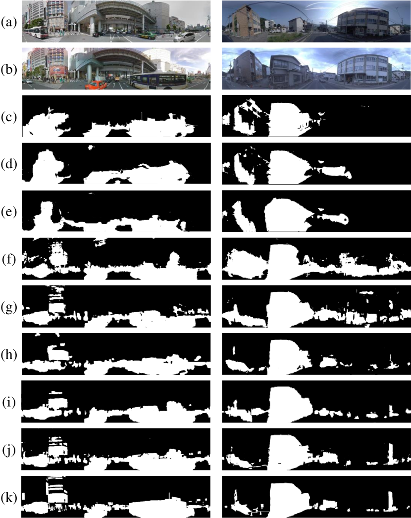
Figure 9: Visual comparison with different methods on the PCD dataset. (a) Image at $t_{0}$, (b) Image at $t_{1}$, (c) CNN-feat [11], (d) DAISY [54], (e) DASC [55], (f) DN [21], (g) CosimNet [9], (h) DOF-CDNet [7], (i) CSCDNet [8], (j) Ours, (k) Ground Truth.

Data Preprocessing. (i) For the PCD dataset, it contains 200 panoramic image pairs, each of which has a 224$\times$1024 resolution. To train our model, we crop the original image by sliding 56 pixels in width, hence each panoramic image will generate 15 patches with a $224\times 224$ resolution. After the plane rotation and mirror, 24000 image pairs are generated in total. Following previous works, we adopt 5-fold cross-validation for model training and testing.

(ii) For the VL-CMU-CD dataset, we also perform data augmentation with the plane rotation and mirror, as the PCD dataset. During the training procedure, we resize the paired images to 512$\times$512. We follow the official split [21], using 933/429 for training and testing. Note that we reduce the multi-class labeling mask to a binary change map, because we focus on change regions instead of class information.

(iii) CDnet2014 consists of 53 moving video sequences but not each image is labeled with a pixel-wise ground-truth. In terms of the evaluations on CDnet2014, we strictly follow previous works, especially the CosimNet [9], to conduct experiments including the selection of image pairs, the split of training/validation set and the process of testing. Following the CosimNet, we selected the background images (i.e., without any foreground objects) as the reference image at time $t_{0}$ and others as the query images at $t_{1}$. The CDnet2014 includes 53 video sequences in different scenarios. We used the annotated frames to built a total of 91595 image pairs, which consist of a training set and a validation set with 73276 pairs and 18319 for each. As suggested by the CDnet2014 benchmark, we evaluate our model on the test set of CDnet2014. Specifically, the image without any change-inducing object is selected as one of the comparison images at time $t_{0}$, and others as the image at time $t_{1}$. All images are resized to 512$\times$512 during training and validating.

Parameter Settings. For the experiment, the proposed framework is initialized from the VGG-16 model[33], which was pre-trained on the ImageNet dataset [52]. The weights of other new layers are initialized by the “xavier” method [56]. In the training phase, we use the the standard Stochastic Gradient Descent (SGD) [31] optimizer. We set the batch size to 8 and the base learning rate to $1e^{-2}$. The momentum is set to 0.95 and weight decay to $1.25e^{-4}$. After 200 epochs, the training procedure converged. We will release the source codes upon acceptance of this work.

V Experimental Results

V-A Evaluation on The PCD Dataset

Tab. II shows the quantitative results on the PCD dataset. It can be seen that the F-Score of our framework is higher than other baseline methods. More specifically, our framework achieves a remarkable F-Score (0.776) on the GSV dataset. There is about 4% improvement to the second-best method, i.e., CSCDNet [8]. Besides, our framework also achieves 0.868 on the TSUNAMI dataset, about 1% improvement compared to the CSCDNet.

Note that both the CDNet and DOF-CDNet [7] adopt the U-Net [19] for change detection. Due to the limited representation ability, they show much worse results than our method. The CosimNet [9] also adopts a Siamese network, which is based on a more powerful segmentation model, i.e., the pre-trained Deeplabv2 [50]. However, our method also shows better results than the CosimNet. Several qualitative results are shown in Fig. 9. It can be seen that our framework is able to capture small as well as large change regions (e.g., large buildings, big cars, small pedestrians, slender poles, imperceptible advertising boards).

TABLE II: Quantitative results on the PCD dataset. The best two results are in bold and underline.

Methods	CNN Backbone	F-Score
		GSV	TSUNAMI
Dense SIFT [57]	-	0.528	0.649
DAISY [54]	-	0.377	0.529
DASC [55]	-	0.409	0.622
CNN-feat [11]	AlexNet	0.639	0.724
DN [21]	DeconvNet	0.614	0.774
CosimNet [9]	Deeplabv2	0.692	0.806
CDNet [7]	U-Net	0.693	0.838
DOF-CDNet [7]	U-Net	0.703	0.838
CSCDNet [8]	Res-18	0.738	0.859
HPCFNet (Ours)	VGG-16	0.776	0.868

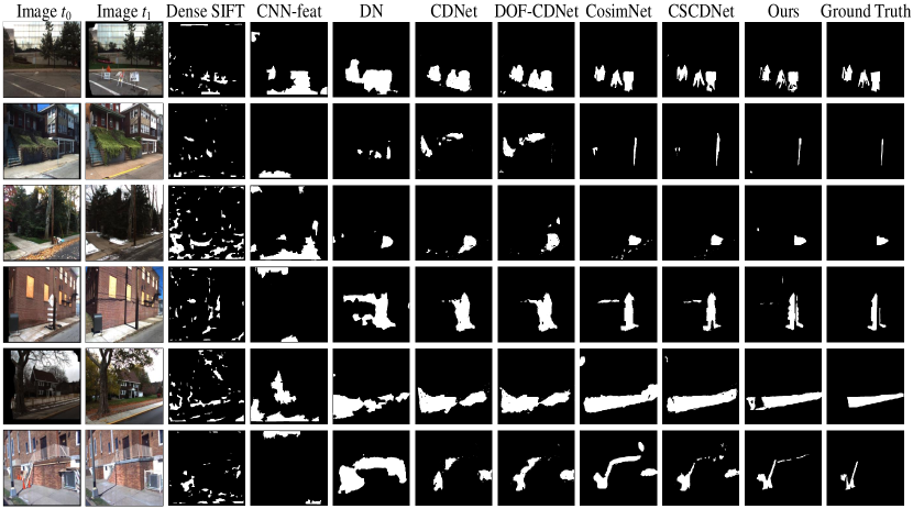
Figure 10: Visual comparisons on the VL-CMU-CD dataset. Our method is good at locating and resolving details.

V-B Evaluation on The VL-CMU-CD Dataset

Tab. III shows the performance of compared methods on the VL-CMU-CD dataset. In terms of F-Score, our framework achieves an accuracy of 0.752, and outperforms the second best CSCDNet [8] by 4.2%. Fig. 10 shows several typical visual results on the VL-CMU-CD dataset. It can be seen that the proposed framework performs well and is visibly better than other methods. Especially, our framework is good at locating and resolving details, e.g, the 1-2 rows of Fig. 10. And it is more accurate on the boundary of changed regions, e.g., the 4 row of Fig. 10.

TABLE III: Quantitative results on the VL-CMU-CD dataset. The best two results are in bold and underline.

Methods	CNN Backbone	Publication	F-Score
Dense SIFT [57]	-	IJCV 2004	0.243
DAISY [54]	-	TPAMI 2009	0.181
DASC [55]	-	CVPR 2015	0.234
CNN-feat [11]	AlexNet	BMVC 2015	0.403
DN [21]	DeconvNet	AR 2018	0.582
CDNet [7]	U-Net	Arxiv 2017	0.685
DOF-CDNet [7]	U-Net	Arxiv 2017	0.688
CosimNet [9]	Deeplabv2	Arxiv 2018	0.706
CSCDNet [8]	Res-18	Arxiv 2018	0.710
HPCFNet (Ours)	VGG-16		0.752

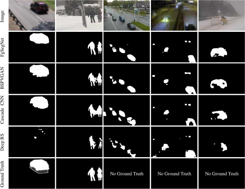
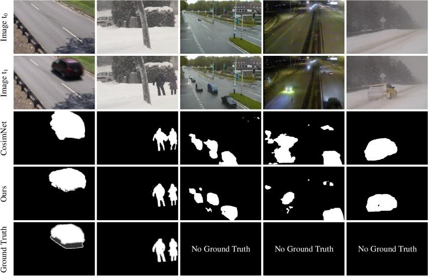
Figure 11: Qualitative results on the CDnet2014 dataset. Top sub-figure: Examples with top-ranked FOE and MOS methods. Bottom sub-figure: Examples with SSCD methods.

V-C Evaluation on The CDnet2014 Dataset

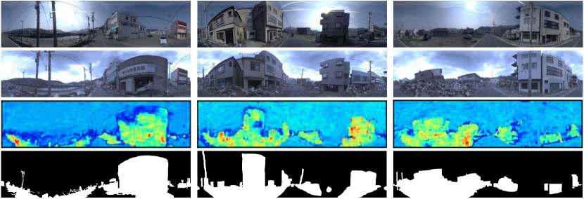
Figure 12: Illustration of Reverse Spatial Attention masks. The first and second rows show the images at $t_{0}$ and $t_{1}$, respectively. The third row shows our RSA masks, and the last row indicates the ground-truths. One can see that the highlighted regions by our RSA module are coarsely consistent to the changed regions.

Tab. IV shows the performance of different methods on the CDnet2014 dataset. The methods at the last two rows are the SSCD methods. Note that the CDnet2014 is essentially created for Foreground Object Extraction (FOE) and Moving Object Segmentation (MOS). In other rows, we also show several top-ranked methods for FOE and MOS. On the tasks of FOE and MOS, researchers mainly devote to segment the foreground object for each frame in video sequence. However, HPCFNet is a method for SSCD aiming to detect the scene change rather than foreground moving objects only. Strictly speaking, CDnet2014 is not a standard dataset for SSCD. Thus, the evaluation performance of HPCFNet is worse than several methods for FOE and MOS. Even though, our framework achieves 0.863 in terms of F-Score, which is very competitive to several methods for FOE and MOS. Besides, two key reasons motivate us to perform experiments on CDnet2014. (a) To the best of our knowledge, CosimNet is the only SSCD method that is evaluated on CDnet2014. To make a fair comparison with CosimNet, we follow it to conduct experiment on CDnet2014. (b) We want to demonstrate that our method is feasible for FOE and MOS on CDnet2014.

Meanwhile, our proposed framework surpasses the CosimNet [9], which shows supreme performance for the SSCD task. The results are reported by the online evaluation server. The qualitative results are shown in Fig. 11. To better verify the generalization, we randomly choose some results from the validating data which are provided ground truths, we also randomly choose some examples from the testing data which have no ground truth. Our method shows outstanding results for images acquired in varying conditions (e.g., hard light, dim light and bad weather).

TABLE IV: Quantitative results on the CDnet2014 dataset. The best two results are in bold and underline.

Task	Methods	F-Score
FOE / MOS	SuBSENSE [58]	0.741
	DeepBS [59]	0.759
	SemanticBGS [60]	0.789
	IUTIS-3 [61]	0.751
	CP3-online [62]	0.792
	Cascade CNN [63]	0.921
	FgSegNet V2 [64]	0.985
	BSPVGAN [65]	0.950
SSCD	CosimNet [9]	0.859
	HPCFNet (Ours)	0.863

V-D Ablation Studies

To demonstrate the benefits of our proposed modules, we conduct additional experiments by adding the modules progressively. Due to the limitation of space, we only exhibit the results on the GSV and TSUNAMI datasets. The other datasets have a similar performance trend. Note that, all the experiments below are based on the VGG-16 backbone.

Effects of PCF modules. To verify the PCF module, a series of experiments are performed, including the framework with concatenation fusion or PCF fusion under different fusion architectures (i.e., early fusion, late fusion and dense fusion). For example, “Early Fusion (Concat)” denotes the early fusion with channel-wise concatenation.

As reported in Tab. V, with the PCF module and a dense fusion, the model improves the performance by a large margin. We here observe that the models with PCF consistently outperform than that of only using the channel concatenation operators. This confirms the effectiveness of our PCF. The main reason is that the fusion method adds additional available information, which enriches the feature representation. Only with one PCF module, our framework (f) achieves the outstanding results on GSV$/$TSUNAMI datasets. It has achieved comparable performance to most deep learning methods. These facts further prove the effectiveness of our proposed method.

TABLE V: Performance comparison on the PCF module. The best results are in bold.

	Methods	F-Score
		GSV		TSUNAMI
(a)	Early Fusion (Concat)	0.694		0.783
(b)	Early Fusion (PCF)	0.712		0.792
(c)	Late Fusion (Concat)	0.718		0.801
(d)	Late Fusion (PCF)	0.726		0.823
(e)	Dense Fusion (Concat)	0.728		0.824
(f)	Dense Fusion (PCF)	0.755		0.857

Effects of the Cross Feature Stack (CFS). To demonstrate the effectiveness of the CFS module, we remove the CFS in PCF and replace with the simple concatenation for comparison. Sufficient experiments are conducted on the basis of three fusion structures: early fusion, late fusion and dense fusion. The comparisons between CFS with concatenation are shown in Table VI. We can see that whichever structure is chosen, CFS enables the boost of performance on both two datasets (GSV and TSUNAMI). This fact indicates that CFS is beneficial for Paired Channel Fusion.

TABLE VI: Performance comparison on the CFS module. The best results are in bold.

Method	Fusion Structure	Fusion Manner	F-Score
			GSV		TSUNAMI
PCF	Early	concatenation	0.701		0.787
		CFS	0.712		0.792
	Late	concatenation	0.720		0.813
		CFS	0.726		0.823
	Dense	concatenation	0.737		0.831
		CFS	0.755		0.857

TABLE VII: Performance comparison on the RSA module. The best results are in bold.

	Methods	F-Score
		GSV		TSUNAMI
(g)	Dense Fusion (PCF)	0.755		0.857
(h)	Dense Fusion (PCF) + RSA	0.761		0.861

Effects of RSA modules. To evaluate the benefits of the proposed RSA modules, we also re-implement our approach with/without them. Tab. VII shows the quantitative performance. In terms of F-Score, our network with RSA modules achieves 0.761/0.861 on GSV/TSUNAMI datasets. Fig. 12 shows the attention masks for a typical street scene pair. We convert the attention masks to heat maps for better visualization. One can see that the highlighted regions by our RSA module are coarsely consistent with the changed regions.

TABLE VIII: The parameters of MPFL and replaced convolutions. $(k,m,n,c)$ represent the kernel size, input channel number, out channel number and group number, respectively.

Location	No. of Parameters	MPFL	Substituted Convolutional Layer
Conv2_2	0.02 MB	(128, 64)	(3, 128, 64, 4)
Conv3_3	0.08 MB	(256, 128)	(3, 256, 128, 4)
Conv4_3	0.34 MB	(512, 256)	(3, 512, 256, 4)
Conv5_3	0.34 MB	(512, 256)	(3, 512, 256, 4)

TABLE IX: Performance comparison on the MPFL strategy. The best results are in bold.

	Methods	F-Score
		GSV		TSUNAMI
(i)	Dense Fusion (PCF) + RSA + Conv	0.764		0.862
(j)	Dense Fusion (PCF) + RSA + 2Conv	0.762		0.859
(k)	Dense Fusion (PCF) + RSA + MPFL $-$ partition	0.768		0.860
($l$)	Dense Fusion (PCF) + RSA + MPFL	0.776		0.868

Effects of the MPFL strategy. The proposed MPFL strategy aims to extract local and global features for adapting to the diverse locations of changed regions. One could suspect that the performance improvement might actually be due to the introduction of additional parameters. For example, whether the performance could also simply be achieved by a convolutional layer with a comparable number of parameters.

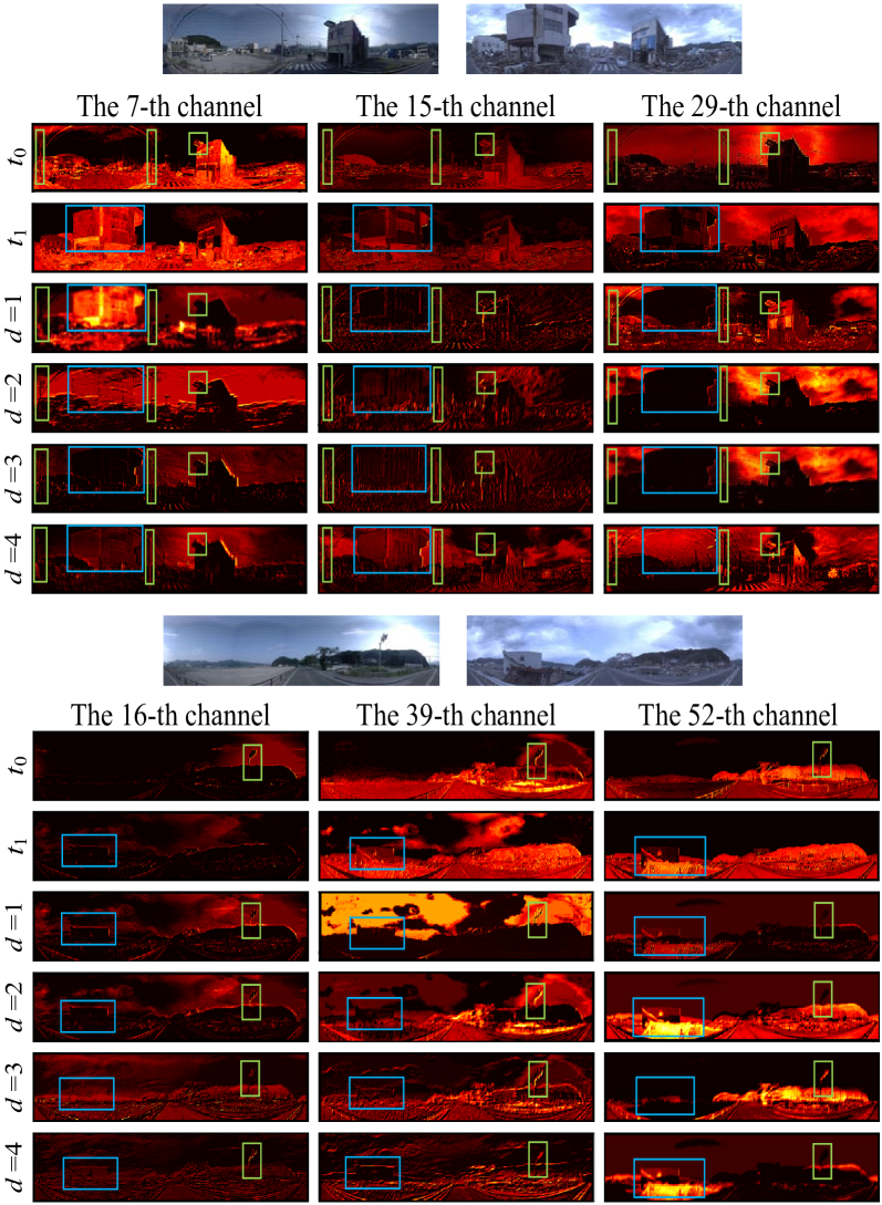
Figure 13: Illustration of PAGC feature maps. For better visualization, we sample several channels from the PAGC module at the Conv1_2 layer. The first row of each sub-figure shows the raw images at $t_{0}$ and $t_{1}$. The second and third rows of each sub-figure show cross feature maps from the paired images. The 4th-7th rows are feature maps generated with different dilation rates $d$. The changed regions at $t_{0}$ and $t_{1}$ are marked by green and blue bounding boxes, respectively.

To address above concerns, we replace the MPFL with convolutional layers which have comparable parameters. More specifically, our MPFL modules at different levels have different parameters. Thus, we use specific convolutional layers to replace the MPFL at each level. Tab. VIII shows structure details. While Tab. IX reports the results with different settings. We observe the following facts: 1) With only one convolutional layer with comparable parameters, the resulting model (model i) achieves 0.764/0.862 F-Score on the GSV/TSUNAMI datasets, respectively. These results are worse than our MPFL strategy (model $l$) which achieves 0.776/0.868. This indicates that our MPFL strategy is more effective. 2) With two additional convolutional layers (model j), the network achieves 0.762/0.859, which are worse than the single convolutional layer (model i). The fact indicates that simply adding parameters is not an effective way for the SSCD task.

Effects of the Partition in MPFL. To demonstrate the effect of Partition, we conducted an ablation experiment by removing the partition step but keeping different-sized convolutions. Note that without partition, each branch contains the intact feature map, hence we remove the multiple independent convolutions and replace it by a single convolution with comparable parameters. For example, four $1\times 1$ convolutions in MPFL (Branch 1) are changed into one $2\times 2$ convolution in the added ablation experiment. As shown in Tab. IX, model without Partition (model k) achieves F-Score of 0.768/0.860 on GSV/TSUNAMI, which is worse than MPFL. MPFL which utilizes partition process has a more powerful capacity of feature learning.

Effects of PAGC. As a key module in PCF, the PAGC plays an important role in capturing the multi-scale correlation between channels. As mentioned in Section III, each channel pair in the group of PAGC contains the information of changed regions. As shown in Fig. 13, the fused feature maps (from the 4-th row to the 7-th in each sub-figure) contain the information of input paired features. Besides, using different dilation rates is able to extract multi-scale feature representations, which enriches the fusion information. These examples confirm the reasonability of our strategy: (1) Fusing features in a channel-wise manner incorporates the information of each paired channels, and enhances the expression of changes at each fused channel. (2) Using different dilation rates enriches the representations of the multi-scale information.

VI Conclusion

In this paper, we propose a novel deep learning framework, named HPCFNet, for the SSCD task. To enhance the feature fusion, we introduce a PCF module to hierarchically fuse feature maps in a channel-wise manner. Next, we propose a RSA module to adaptively highlight the features indicating the changed regions. To enrich the scene information, we also propose a MPFL strategy to extract features in a global-to-local manner. Extensive experiments on three publicly available SSCD datasets (i.e., PCD, VL-CMU-CD and CDnet2014) show that our approach achieves remarkable performance compared to other state-of-the-art methods.

References

- [1] C. Wu, L. Zhang, and B. Du, “Kernel slow feature analysis for scene change detection,” IEEE Transactions on Geoscience and Remote Sensing (TGRS), vol. 55, no. 4, pp. 2367–2384, 2017.
- [2] C. Wu, L. Zhang, and L. Zhang, “A scene change detection framework for multi-temporal very high resolution remote sensing images,” Signal Processing, vol. 124, pp. 184–197, 2016.
- [3] M. Hussain, D. Chen, A. Cheng, H. Wei, and D. Stanley, “Change detection from remotely sensed images: From pixel-based to object-based approaches,” ISPRS Journal of Photogrammetry and Remote Sensing, vol. 80, pp. 91–106, 2013.
- [4] L. Mou, L. Bruzzone, and X. X. Zhu, “Learning spectral-spatial-temporal features via a recurrent convolutional neural network for change detection in multispectral imagery,” IEEE Transactions on Geoscience and Remote Sensing (TGRS), vol. 57, no. 2, pp. 924–935, 2018.
- [5] B. Du, Y. Wang, C. Wu, and L. Zhang, “Unsupervised scene change detection via latent dirichlet allocation and multivariate alteration detection,” IEEE Journal of Selected Topics in Applied Earth Observations and Remote Sensing (JSTARS), vol. 11, no. 12, pp. 4676–4689, 2018.
- [6] C. Wu, B. Du, and L. Zhang, “Slow feature analysis for change detection in multispectral imagery,” IEEE Transactions on Geoscience and Remote Sensing (TGRS), vol. 52, no. 5, pp. 2858–2874, 2013.
- [7] K. Sakurada, W. Wang, N. Kawaguchi, and R. Nakamura, “Dense optical flow based change detection network robust to difference of camera viewpoints,” arXiv:1712.02941, 2017.
- [8] K. Sakurada, “Weakly supervised silhouette-based semantic change detection,” arXiv:1811.11985, 2018.
- [9] E. Guo, X. Fu, J. Zhu, M. Deng, Y. Liu, Q. Zhu, and H. Li, “Learning to measure change: Fully convolutional siamese metric networks for scene change detection,” arXiv:1810.09111, 2018.
- [10] S. H. Khan, X. He, F. Porikli, M. Bennamoun, F. Sohel, and R. Togneri, “Learning deep structured network for weakly supervised change detection,” arXiv:1606.02009, 2016.
- [11] K. Sakurada and T. Okatani, “Change detection from a street image pair using cnn features and superpixel segmentation,” in Proceedings of the British Machine Vision Conference (BMVC), 2015, pp. 61–73.
- [12] P. Rosin, “Thresholding for change detection,” in Proceedings of the IEEE International Conference on Computer Vision (ICCV), 1998, pp. 274–279.
- [13] P. L. Rosin and E. Ioannidis, “Evaluation of global image thresholding for change detection,” Pattern Recognition Letters (PRL), vol. 24, no. 14, pp. 2345–2356, 2003.
- [14] T. Pollard and J. L. Mundy, “Change detection in a 3-d world,” in Proceedings of the IEEE Computer Vision and Pattern Recognition (CVPR), 2007, pp. 1–6.
- [15] G. Schindler and F. Dellaert, “Probabilistic temporal inference on reconstructed 3d scenes,” in Proceedings of the IEEE Computer Vision and Pattern Recognition (CVPR), 2010, pp. 1410–1417.
- [16] A. Taneja, L. Ballan, and M. Pollefeys, “Image based detection of geometric changes in urban environments,” in Proceedings of IEEE International Conference on Computer Vision (ICCV), 2011, pp. 2336–2343.
- [17] ——, “City-scale change detection in cadastral 3D models using images,” in Proceedings of the IEEE Computer Vision and Pattern Recognition (CVPR), 2013, pp. 113–120.
- [18] J. Long, E. Shelhamer, and T. Darrell, “Fully convolutional networks for semantic segmentation,” in Proceedings of the IEEE Computer Vision and Pattern Recognition (CVPR), 2015, pp. 3431–3440.
- [19] O. Ronneberger, P. Fischer, and T. Brox, “U-net: Convolutional networks for biomedical image segmentation,” in Proceedings of the International Conference on Medical Image Computing and Computer-Assisted Intervention (MICCAI). Springer, 2015, pp. 234–241.
- [20] C. Szegedy, W. Liu, Y. Jia, P. Sermanet, S. Reed, D. Anguelov, D. Erhan, V. Vanhoucke, and A. Rabinovich, “Going deeper with convolutions,” in Proceedings of the IEEE Computer Vision and Pattern Recognition (CVPR), 2015, pp. 1–9.
- [21] P. F. Alcantarilla, S. Stent, G. Ros, R. Arroyo, and R. Gherardi, “Street-view change detection with deconvolutional networks,” Autonomous Robots, vol. 42, no. 7, pp. 1301–1322, 2018.
- [22] P. Zhang, W. Liu, Y. Lei, H. Wang, and H. Lu, “Rapnet: Residual atrous pyramid network for importance-aware street scene parsing,” IEEE Transactions on Image Processing (TIP), vol. 29, pp. 5010–5021, 2020.
- [23] Y. Wang, P.-M. Jodoin, F. Porikli, J. Konrad, Y. Benezeth, and P. Ishwar, “Cdnet 2014: an expanded change detection benchmark dataset,” in Proceedings of the IEEE Computer Vision and Pattern Recognition Workshops (CVPRW), 2014, pp. 387–394.
- [24] P. Zhang, W. Liu, Y. Lei, H. Wang, and H. Lu, “Deep multiphase level set for scene parsing,” IEEE Transactions on Image Processing (TIP), vol. 29, pp. 4556–4567, 2020.
- [25] P. Zhang, W. Liu, Y. Lei, and H. Lu, “Hyperfusion-net: Hyper-densely reflective feature fusion for salient object detection,” Pattern Recognition (PR), vol. 93, pp. 521–533, 2019.
- [26] P. Zhang, W. Liu, Y. Lei, H. Lu, and X. Yang, “Cascaded context pyramid for full-resolution 3d semantic scene completion,” in Proceedings of the IEEE International Conference on Computer Vision (ICCV), 2019, pp. 7801–7810.
- [27] P. Zhang, W. Liu, H. Lu, and C. Shen, “Salient object detection by lossless feature reflection,” International Joint Conference on Artificial Intelligence (IJCAI), vol. 14, no. 4, pp. 1149–1155, 2018.
- [28] Y. Ma, Y. Guo, H. Liu, Y. Lei, and G. Wen, “Global context reasoning for semantic segmentation of 3d point clouds,” in Proceedings of the IEEE Winter Conference on Applications of Computer Vision (WACV), 2020, pp. 2931–2940.
- [29] R. J. Radke, S. Andra, O. Al-Kofahi, and B. Roysam, “Image change detection algorithms: a systematic survey,” IEEE Transactions on Image Processing (TIP), vol. 14, no. 3, pp. 294–307, 2005.
- [30] K. He, X. Zhang, S. Ren, and J. Sun, “Deep residual learning for image recognition,” in Proceedings of the IEEE Computer Vision and Pattern Recognition (CVPR), 2016, pp. 770–778.
- [31] A. Krizhevsky, I. Sutskever, and G. E. Hinton, “Imagenet classification with deep convolutional neural networks,” in Proceedings of the Advances in Neural Information Processing Systems (NuerIPS), 2012, pp. 1097–1105.
- [32] Y. LeCun, L. Bottou, Y. Bengio, P. Haffner et al., “Gradient-based learning applied to document recognition,” Proceedings of the IEEE, vol. 86, no. 11, pp. 2278–2324, 1998.
- [33] K. Simonyan and A. Zisserman, “Very deep convolutional networks for large-scale image recognition,” arXiv:1409.1556, 2014.
- [34] Y. Liu, L. Liu, P. Wang, P. Zhang, and Y. Lei, “Semi-supervised crowd counting via self-training on surrogate tasks,” in Proceedings of the European Conference on Computer Vision (ECCV). Springer, 2020.
- [35] Y. Lei, Y. Liu, P. Zhang, and L. Liu, “Towards using count-level weak supervision for crowd counting,” Pattern Recognition (PR), vol. 109, p. 107616, 2021.
- [36] Y. Zhan, K. Fu, M. Yan, X. Sun, H. Wang, and X. Qiu, “Change detection based on deep siamese convolutional network for optical aerial images,” IEEE Geoscience and Remote Sensing Letters (GRSL), vol. 14, no. 10, pp. 1845–1849, 2017.
- [37] P. Zhang, W. Liu, H. Lu, and C. Shen, “Salient object detection with lossless feature reflection and weighted structural loss,” IEEE Transactions on Image Processing (TIP), vol. 28, no. 6, pp. 3048–3060, 2019.
- [38] L. Itti and C. Koch, “Computational modelling of visual attention,” Nature Reviews Neuroscience, vol. 2, no. 3, p. 194, 2001.
- [39] L. Itti, C. Koch, and E. Niebur, “A model of saliency-based visual attention for rapid scene analysis,” IEEE Transactions on Pattern Analysis and Machine Intelligence (TPAMI), no. 11, pp. 1254–1259, 1998.
- [40] B. A. Olshausen, C. H. Anderson, and D. C. Van Essen, “A neurobiological model of visual attention and invariant pattern recognition based on dynamic routing of information,” Journal of Neuroscience, vol. 13, no. 11, pp. 4700–4719, 1993.
- [41] P. Zhang, W. Liu, H. Wang, Y. Lei, and H. Lu, “Deep gated attention networks for large-scale street-level scene segmentation,” Pattern Recognition (PR), vol. 88, pp. 702–714, 2019.
- [42] H. Larochelle and G. E. Hinton, “Learning to combine foveal glimpses with a third-order boltzmann machine,” in Proceedings of the Advances in Neural Information Processing Systems (NuerIPS), 2010, pp. 1243–1251.
- [43] V. Mnih, N. Heess, A. Graves et al., “Recurrent models of visual attention,” in Proceedings of the Advances in Neural Information Processing Systems (NuerIPS), 2014, pp. 2204–2212.
- [44] M. Jaderberg, K. Simonyan, A. Zisserman et al., “Spatial transformer networks,” in Proceedings of the Advances in Neural Information Processing Systems (NuerIPS), 2015, pp. 2017–2025.
- [45] J. Fu, J. Liu, H. Tian, Y. Li, Y. Bao, Z. Fang, and H. Lu, “Dual attention network for scene segmentation,” in Proceedings of the IEEE Conference on Computer Vision and Pattern Recognition (CVPR), 2019, pp. 3146–3154.
- [46] S. Chen, X. Tan, B. Wang, and X. Hu, “Reverse attention for salient object detection,” in Proceedings of the European Conference on Computer Vision (ECCV). Springer, 2018, pp. 234–250.
- [47] C. Cao, X. Liu, Y. Yang, Y. Yu, J. Wang, Z. Wang, Y. Huang, L. Wang, C. Huang, W. Xu et al., “Look and think twice: Capturing top-down visual attention with feedback convolutional neural networks,” in Proceedings of the IEEE Computer Vision and Pattern Recognition (CVPR), 2015, pp. 2956–2964.
- [48] J. Hu, L. Shen, and G. Sun, “Squeeze-and-excitation networks,” in Proceedings of the IEEE Computer Vision and Pattern Recognition (CVPR), 2018, pp. 7132–7141.
- [49] S. Woo, J. Park, J.-Y. Lee, and I. So Kweon, “Cbam: Convolutional block attention module,” in Proceedings of the European Conference on Computer Vision (ECCV). Springer, 2018, pp. 3–19.
- [50] L.-C. Chen, G. Papandreou, I. Kokkinos, K. Murphy, and A. L. Yuille, “Deeplab: Semantic image segmentation with deep convolutional nets, atrous convolution, and fully connected crfs,” IEEE Transactions on Pattern Analysis and Machine Intelligence (TPAMI), vol. 40, no. 4, pp. 834–848, 2017.
- [51] S. Ioffe and C. Szegedy, “Batch normalization: Accelerating deep network training by reducing internal covariate shift,” in International Conference on Machine Learning (ICML), 2015, pp. 448–456.
- [52] J. Deng, W. Dong, R. Socher, L.-J. Li, K. Li, and L. Fei-Fei, “Imagenet: A large-scale hierarchical image database,” in Proceedings of the IEEE Computer Vision and Pattern Recognition (CVPR), 2009, pp. 248–255.
- [53] A. Paszke, S. Gross, S. Chintala, G. Chanan, E. Yang, Z. DeVito, Z. Lin, A. Desmaison, L. Antiga, and A. Lerer, “Automatic differentiation in pytorch,” 2017.
- [54] E. Tola, V. Lepetit, and P. Fua, “Daisy: An efficient dense descriptor applied to wide-baseline stereo,” IEEE Transactions on Pattern Analysis and Machine Intelligence (TPAMI), vol. 32, no. 5, pp. 815–830, 2009.
- [55] S. Kim, D. Min, B. Ham, S. Ryu, M. N. Do, and K. Sohn, “Dasc: Dense adaptive self-correlation descriptor for multi-modal and multi-spectral correspondence,” in Proceedings of the IEEE Computer Vision and Pattern Recognition (CVPR), 2015, pp. 2103–2112.
- [56] X. Glorot and Y. Bengio, “Understanding the difficulty of training deep feedforward neural networks,” in Proceedings of the International Conference on Artificial Intelligence and Statistics (AISTATS). Citeseer, 2010, pp. 249–256.
- [57] D. G. Lowe, “Distinctive image features from scale-invariant keypoints,” International Journal of Computer Vision (IJCV), vol. 60, no. 2, pp. 91–110, 2004.
- [58] P.-L. St-Charles, G.-A. Bilodeau, and R. Bergevin, “Subsense: A universal change detection method with local adaptive sensitivity,” IEEE Transactions on Image Processing (TIP), vol. 24, no. 1, pp. 359–373, 2014.
- [59] M. Babaee, D. T. Dinh, and G. Rigoll, “A deep convolutional neural network for video sequence background subtraction,” Pattern Recognition (PR), vol. 76, pp. 635–649, 2018.
- [60] M. Braham, S. Piérard, and M. Van Droogenbroeck, “Semantic background subtraction,” in Proceedings of the IEEE International Conference on Image Processing (ICIP), 2017, pp. 4552–4556.
- [61] S. Bianco, G. Ciocca, and R. Schettini, “Combination of video change detection algorithms by genetic programming,” IEEE Transactions on Evolutionary Computation (TEC), vol. 21, no. 6, pp. 914–928, 2017.
- [62] D. Liang, M. Hashimoto, K. Iwata, X. Zhao et al., “Co-occurrence probability-based pixel pairs background model for robust object detection in dynamic scenes,” Pattern Recognition (PR), vol. 48, no. 4, pp. 1374–1390, 2015.
- [63] Y. Wang, Z. Luo, and P.-M. Jodoin, “Interactive deep learning method for segmenting moving objects,” Pattern Recognition Letters (PRL), vol. 96, pp. 66–75, 2017.
- [64] L. A. Lim and H. Y. Keles, “Learning multi-scale features for foreground segmentation,” Pattern Analysis and Applications, vol. 23, no. 3, pp. 1369–1380, 2020.
- [65] W. Zheng, K. Wang, and F.-Y. Wang, “A novel background subtraction algorithm based on parallel vision and bayesian gans,” Neurocomputing, vol. 394, pp. 178–200, 2020.