Causal Inference for Nonlinear Outcome Models with Possibly Invalid Instrumental Variables

Instrumental variable methods are widely used for inferring the causal effect in the presence of unmeasured confounders. Existing instrumental variable methods for nonlinear outcome models require stringent identifiability conditions. This paper considers a flexible semi-parametric potential outcome model that allows for possibly invalid instruments. We propose new identifiability conditions to identify the causal parameters when the majority of the instrumental variables are valid. We devise a novel inference procedure for a new average structural function and the conditional average treatment effect. We establish the asymptotic normality of the proposed estimators and construct confidence intervals for the causal estimands by bootstrap. The proposed method is demonstrated in large-scale simulation studies and is applied to infer the effect of income on house ownership.

Keywords: unmeasured confounders; binary outcome; semi-parametric model; endogeneity; partial mean

JEL classification code: C36

1 Introduction

Unmeasured confounders are significant concerns for inferring causal effects from observational studies. The instrumental variable (IV) approach is the state-of-the-art method for estimating the causal effects in the presence of unmeasured confounders (Wooldridge, 2010, e.g.). The success of IV-based methods requires the IVs to satisfy three core conditions: conditioning on the observed covariates,
(A1) the IVs are associated with the exposure;
(A2) the IVs have no direct effects on the outcome;
(A3) the IVs are independent of unmeasured confounders.

A significant challenge of applying IV-based methods is to identify valid instruments simultaneously satisfying (A1)-(A3) (Murray, 2006; Conley et al., 2012, e.g.). Since (A2) and (A3) cannot be tested in a data-dependent way, it requires strong domain knowledge to identify valid IVs. In many applications, the relationship between the outcome and treatment is nonlinear. For example, when the outcome is binary, the treatment affects the outcome in a nonlinear way. Inference for the causal effect under the nonlinear outcome models is more challenging than that for the linear model. There is a pressing need to develop accurate causal inference methods in nonlinear outcome models with possibly invalid instruments.

1.1 Existing works

Semi-parametric approaches are widely used for causal inference with nonlinear outcome models. Blundell and Powell (2004) and Rothe (2009) considered the double-index models for binary outcomes by assuming a valid control function and made inferences for the model parameters. In practice, it may be more interesting to make inferences for the conditional average treatment effect (CATE) and the average structural function (ASF) (Blundell and Powell, 2003), which are measured on the same scale as the outcome variable. Hahn and Ridder (2013) studied the influence function of partial means estimators with semi-parametric outcome models and generated covariates. A typical example for generated covariates is a valid control function. By assuming a valid control function, the ASF can be estimated via the partial means method (Newey, 1994) and its asymptotic properties have been studied in Mammen et al. (2012). However, the violations of the valid control function assumption are barely studied in the semi-parametric outcome models.

For causal inference with binary responses, parametric models such as probit and logistic outcome models (Rivers and Vuong, 1988; Vansteelandt et al., 2011) were studied with valid control functions and IVs. In recent work, Carlson (2021) considered causal inference in a probit outcome model and a parametric treatment model. They relaxed the valid control function condition in Rivers and Vuong (1988) and allowed the unobserved confounders to depend on the IVs through a specific form. However, these parametric models required specific distributions of the unmeasured confounders, which can be misspecified in practical applications. The mixed-logistic model, stated in the following equation (30), is commonly used in observational studies (Clarke and Windmeijer, 2012). However, even assuming a valid IV, the two-stage method is known to be biased for the mixed-logistic model (Cai et al., 2011) .

Under linear outcome models, some recent progress has been made in inferring the causal effects with possibly invalid IVs. With continuous outcome and exposure models, Kolesár et al. (2015) and Bowden et al. (2015) proposed methods in the setting that all candidate IVs can be invalid, but the IV strength and the direct effect on the outcome are nearly orthogonal. Bowden et al. (2016), Kang et al. (2016), and Windmeijer et al. (2019) proposed consistent estimators of causal effects assuming at least 50% of the IVs are valid. Hartwig et al. (2017) and Guo et al. (2018) considered linear outcome models assuming that the most common causal effect estimate is a consistent estimate of the true causal effect. Under this assumption, Guo et al. (2018) constructed confidence intervals for the treatment effect, and Windmeijer et al. (2019) further developed the inference procedure built on Guo et al. (2018). However, these methods are developed under the linear models and do not apply to nonlinear outcome models.

In the GMM framework, Liao (2013); Cheng and Liao (2015); Caner et al. (2018) assumed the prior knowledge of a set of valid moments and considered selecting valid moments among another set of moments. DiTraglia (2016) leveraged invalid moments to reduce the mean squared error with the prior knowledge of a set of valid moments. In contrast, the current paper does not assume any prior knowledge of the validity of any given instrument.

1.2 Our results and contributions

We propose a robust causal inference method for semi-parametric outcome models with possibly invalid IVs. We relax the valid control function condition (Condition 2.1 in Section 2.1) by allowing for a violation in a semi-parametric form. It generalizes the linear violation forms considered in linear outcome models (Kang et al., 2016; Guo et al., 2018, e.g.).

We impose the dimension reduction condition (Condition 2.2 in Section 2.2) and the majority rule (Condition 2.3 in Section 2.2) as new identification conditions for semi-parametric outcome models with possibly invalid IVs. These new identifiability conditions significantly weaken the commonly used Condition 2.1. We show that the new identifiability conditions are sufficient to identify a new ASF and CATE.

We propose a three-step inference procedure for CATE in Semi-parametric outcome models with possibly invalid IVs, termed as SpotIV. First, we estimate the reduced-form parameters based on the existing dimension reduction methods. Second, we apply the median estimator to estimate the model parameters by leveraging that more than $50\%$ of candidate IVs are valid. Third, we develop a partial mean estimator for the causal estimand of interest. We further develop a self-checking method to partially test whether the majority rule is satisfied.

We establish the asymptotic normality of our proposed estimator and construct confidence intervals for the causal estimands by bootstrap. We demonstrate our proposed method in simulations and apply the method to infer the causal effects of household income on whether a family owns a house based on the China Family Panel Studies (CFPS).

1.3 Organization of the rest of the paper

The rest of this paper is organized as follows. In Section 2, we introduce the model and identifiability conditions. In Section 3, the SpotIV estimator is proposed to make inference for ASF and CATE. Section 4 provides theoretical guarantees for the proposed method. In Section 5, we investigate the empirical performance of the SpotIV estimator. In Section 6, the SpotIV estimator is applied to infer the income’s causal effects on house ownership.

2 Nonlinear outcome models and identifiability conditions

For the $i$-th subject, let $y_{i}\in\mathbb{R}$ denote the observed outcome, $d_{i}\in\mathbb{R}$ denote the exposure or the treatment, $z_{i}\in\mathbb{R}^{p_{z}}$ denote a set of candidate IVs, and $x_{i}\in\mathbb{R}^{p_{x}}$ denote baseline covariates. Define $p:=p_{z}+p_{x}$ and we use $w_{i}:=(z_{i}^{\intercal},x_{i}^{\intercal})^{\intercal}\in\mathbb{R}^{p}$ to denote all the measured covariates, including candidate IVs and baseline covariates. We assume that the data $\{y_{i},d_{i},w_{i}\}_{1\leq i\leq n}$ are generated in i.i.d. fashions. Let $u_{i}$ denote the unmeasured confounder which can be associated with both exposure and outcome variables.

We define causal effects using the potential outcome framework (Neyman, 1923; Rubin, 1974). Let $y_{i}^{(d)}\in\mathbb{R}$ be the potential outcome if the $i$-th individual were to have exposure $d$. We consider the following nonlinear potential outcome model

$$\mathbb{E}[y^{(d)}_{i}|w_{i}=w,u_{i}=u]:=q\left(d\beta+w^{\intercal}\kappa,u\right),$$ (1)

where $q:\mathbb{R}^{2}\rightarrow\mathbb{R}$ is a link function, $\beta\in\mathbb{R}$ is the coefficient corresponding to the exposure, and $\kappa=(\kappa_{z}^{\intercal},\kappa_{x}^{\intercal})^{\intercal}\in\mathbb{R}^{p}$ is the coefficient vector corresponding to both the IVs and baseline covariates. The function $q$ can be either known or unknown. Model (1) includes a broad class of nonlinear potential outcome models for both continuous and binary outcomes. For binary outcomes, if $q(a,b)=1/(1+\exp(-a-b))$, then (1) is the mixed-logistic model (Vansteelandt et al., 2011); if $q(a,b)=\mathbbm{1}(a+b>0)$ and $u_{i}$ is normal with mean zero, then (1) is the probit model (Rivers and Vuong, 1988).

We assume that $y_{i}^{(d)}\;\raisebox{0.50003pt}{\rotatebox[origin={c}]{90.0}{$\models$}}\;d_{i}\mid(w_{i}^{\intercal},u_{i})$. This condition is mild as we can always identify an unmeasured variable $u_{i}$ such that $y_{i}^{(d)}$ and $d_{i}$ are conditionally independent. This is much weaker than the (strong) ignorability condition $y_{i}^{(d)}\;\raisebox{0.50003pt}{\rotatebox[origin={c}]{90.0}{$\models$}}\;d_{i}\mid w_{i}$ (Rosenbaum and Rubin, 1983). Under the condition $y_{i}^{(d)}\;\raisebox{0.50003pt}{\rotatebox[origin={c}]{90.0}{$\models$}}\;d_{i}\mid(w_{i}^{\intercal},u_{i})$ and the consistency assumption (Imbens and Rubin, 2015, e.g.), we connect the conditional outcome model and the potential outcome model (1) as

$$\mathbb{E}[y_{i}|d_{i}=d,w_{i}=w,u_{i}=u]=\mathbb{E}[y^{(d)}_{i}|d_{i}=d,w_{i}=w,u_{i}=u]=\mathbb{E}[y^{(d)}_{i}|w_{i}=w,u_{i}=u].$$ (2)

Consequently, the potential outcome model (1) leads to the following outcome model,

$$\mathbb{E}[y_{i}|d_{i}=d,w_{i}=w,u_{i}=u]=q\left(d\beta+w^{\intercal}\kappa,u\right).$$ (3)

For the exposure $d_{i}$, we consider a linear working model

$$d_{i}=w_{i}^{\intercal}\gamma+v_{i}~{}~{}\text{with}~{}~{}\gamma=(\mathbb{E}[w_{i}w_{i}^{\intercal}])^{-1}\mathbb{E}[w_{i}d_{i}]~{}~{}\text{and}~{}~{}\mathbb{E}[w_{i}v_{i}]=0.$$ (4)

When there exist unmeasured confounders, $u_{i}$ and $v_{i}$ are correlated, and the exposure is endogenous; that is, $d_{i}$ is associated with the unmeasured confounder $u_{i}$ even after conditioning on the measured variables $w_{i}$; see Figure 1 for an illustration.

2.1 Review of the control function approach with valid IVs

We first review the control function approach with valid IVs, which is widely adopted for causal inference with nonlinear outcome models (Rivers and Vuong, 1988; Blundell and Powell, 2004; Rothe, 2009; Petrin and Train, 2010; Cai et al., 2011; Wooldridge, 2015; Guo and Small, 2016). The key idea is to treat the residual $v_{i}$ of the exposure model (4) as a proxy for the unmeasured confounders. Then $v_{i}$ is included in the outcome model as an adjustment for the unmeasured confounder. The success of the control function method relies on the following identifiability condition (Blundell and Powell, 2004; Rothe, 2009).

Condition 2.1 (Control function with valid IVs).

The IV strength $\gamma_{z}$ in (4) satisfies $\|\gamma_{z}\|_{2}\geq\tau_{0}>0$ for a positive constant $\tau_{0}$. The direct effect $\kappa_{z}$ in (3) is equal to zero. The conditional density $f_{u}(u_{i}|w_{i},v_{i})$ satisfies

$$f_{u}(u_{i}|w_{i},v_{i})=f_{u}(u_{i}|v_{i}).$$ (5)

The condition $\|\gamma_{z}\|_{2}\geq\tau_{0}>0$ assumes strong associations between the IVs and the exposure variable, which corresponds to the IV assumption (A1). The condition $\kappa_{z}=0$ assumes that the IVs do not directly affect the outcome, which corresponds to (A2). Equation (5) assumes that conditioning on the control variable $v_{i}$, the unmeasured confounder $u_{i}$ is independent of the measured covariates $w_{i}$. Note that (5) automatically holds if the errors $(u_{i},v_{i})$ are independent of $w_{i}.$ The assumption in (5) can be viewed as a version of (A3) for nonlinear outcome models. If $v_{i}$ is independent of $w_{i}$, then condition (5) implies (A3). However, such a connection may not hold in general. Under Condition 2.1, the outcome model (3) implies

$$\mathbb{E}[y_{i}|d_{i},w_{i},v_{i}]=\int q(d_{i}\beta+w_{i}^{\intercal}\kappa,u_{i})f_{u}(u_{i}|v_{i})du_{i}:=g_{0}\left(d_{i}\beta+x_{i}^{\intercal}\kappa_{x},v_{i}\right),$$ (6)

where the function $g_{0}:\mathbb{R}^{2}\rightarrow\mathbb{R}$ is induced by the functions $q(\cdot,\cdot)$ and $f_{u}(\cdot)$. Inference for parameters $\beta$ and $\kappa_{x}$ in (6) has been studied in Blundell and Powell (2004) and Rothe (2009). For nonlinear outcome models, Blundell and Powell (2003) proposed the average structural function (ASF) as the targeted causal estimand, defined as

$$\textrm{ASF}(d,w)=\mathbb{E}_{u_{i}}[q(d\beta+w^{\intercal}\kappa,u_{i})].$$ (7)

Under Condition 2.1, it holds that

$$\textrm{ASF}(d,w)=\mathbb{E}[\mathbb{E}[q(d\beta+w^{\intercal}\kappa,u_{i})|v_{i}]]=\mathbb{E}[g_{0}\left(d\beta+x^{\intercal}\kappa_{x},v_{i}\right)],$$ (8)

where the last step follows from (6). Mammen et al. (2012); Hahn and Ridder (2013) proposed partial mean estimators of ASF$(d,w)$ by leveraging the last expression in (8).

We shall highlight that Condition 2.1 can be easily violated in practical applications. First, the assumption (5) is unlikely to hold when $u_{i}$ involves omitted variables, which may be associated with measured covariates $w_{i}$. As pointed out in Blundell and Powell (2004), a control function satisfying Condition 2.1 largely relies on including all the suspicious confounders in the model, which may be a strong assumption for practical applications. Second, Carlson (2021) pointed out that the assumption (5) does not allow heteroskedasticity with respect to the distribution of $u_{i}$. For example, the model of $u_{i}|w_{i},v_{i}$ specified in the following equation (11) violates Condition 2.1. Finally, the no direct effect assumption ($\kappa_{z}=0$) might be violated in practice. Indeed, both $\kappa_{z}=0$ and the assumption (5) cannot be tested in a data-dependent way. The above discussions strongly motivate us to propose much weaker identification conditions in the following subsection.

2.2 New identifiability conditions

We introduce new identifiability conditions, which weakens Condition 2.1.

Condition 2.2 (Dimension reduction).

The direct effect $\kappa_{z}$ in (3) can be non-zero. There exists some $\eta\in\mathbb{R}^{p\times p_{\eta}}$ for $0\leq p_{\eta}<p$ such that the conditional density $f_{u}(u_{i}|w_{i},v_{i})$ satisfies

$$f_{u}(u_{i}|w_{i},v_{i})=f_{u}(u_{i}|w_{i}^{\intercal}\eta,v_{i}).$$ (9)

Without loss of generality, we assume the columns of $\eta$ are linearly independent and $p_{\eta}<p$. In contrast to (5), the model (9) allows the unmeasured confounder $u_{i}$ to depend on the measured covariates $w_{i}$ through the linear transformations $w_{i}^{\intercal}\eta$, after conditioning on $v_{i}$. Condition 2.2 essentially requires a dimension reduction property of the conditional density $f_{u}(u_{i}|w_{i},v_{i})$. As illustrated in Figure 1, Condition 2.2 relaxes Condition 2.1 by allowing $\kappa_{z}\neq\bm{0}$ and $\eta\neq\bm{0}$.

Figure 1: Relaxation of assumptions $\kappa_{z}=0$ and (5) in Condition 2.1.

In view of (9), the conditional mean of the outcome can be written as

$$\mathbb{E}[y_{i}|d_{i},w_{i},v_{i}]=\int q(d_{i}\beta+w_{i}^{\intercal}\kappa,u_{i})f_{u}(u_{i}|w_{i}^{\intercal}\eta,v_{i})du_{i}:=g^{*}\left(d_{i}\beta+w_{i}^{\intercal}\kappa,w_{i}^{\intercal}\eta,v_{i}\right)$$ (10)

for $g^{*}:\mathbb{R}^{p_{\eta}+2}\rightarrow\mathbb{R}$. In comparison to (6), expression (10) allows the direct effects $\kappa_{z}\neq\bm{0}$ and additional indices $w_{i}^{\intercal}\eta$, which are induced by the dependence of $u_{i}$ and $w_{i}^{\intercal}\eta$ as in (9).

We introduce an extra identifiability condition, which requires a majority of the candidate IVs to be valid. We use $\mathcal{S}$ to denote the set of relevant IVs and $\mathcal{V}$ to denote the set of valid IVs, i.e.,

$$\mathcal{S}=\{1\leq j\leq p_{z}:\gamma_{j}\neq 0\}\quad\text{and}\quad\mathcal{V}=\{j\in\mathcal{S}:\kappa_{j}=0,\eta_{j,.}=\bm{0}\}.$$

The set $\mathcal{S}$ contains all candidate IVs strongly associated with the exposure. The set $\mathcal{V}$ is a subset of $\mathcal{S}$. Notice that the IVs in set $\mathcal{V}$ have no direct effects on the outcome and are independent of the unmeasured confounder $u_{i}$ conditioning on $(z_{i,\mathcal{V}^{c}}^{\intercal},x_{i}^{\intercal},v_{i})$. Hence, we refer to $\mathcal{V}$ as the set of valid IVs and $\mathcal{V}^{c}$ as the set of invalid IVs.

When the candidate IVs are possibly invalid, the main challenge is that the set $\mathcal{V}$ is unknown a priori in data analysis. The following identifiability condition is needed to identify the causal effect without prior knowledge of the set of valid IVs.

Condition 2.3 (Majority rule).

More than half of the relevant IVs are valid:

$$\left|\mathcal{V}\right|>\left|\mathcal{S}\cap\mathcal{V}^{c}\right|.$$

The majority rule assumes that more than half of the relevant IVs are valid but does not require prior knowledge of the set $\mathcal{V}$. The majority rule has been proposed in linear outcome models with invalid IVs (Bowden et al., 2016; Kang et al., 2016; Guo et al., 2018; Windmeijer et al., 2019). In this work, we generalize the majority rule into a semi-parametric format.

To summarize, Conditions 2.2 and 2.3 are new identifiability conditions to identify causal effects in the semi-parametric outcome model (1) with possibly invalid IVs. These two conditions weaken Condition 2.1 and better accommodate for practical applications. Below we review two existing relaxations of Condition 2.1 considered in the literature.

Remark 2.1 (Relaxation in probit models).

Along the line of probit outcome models, Rivers and Vuong (1988) assumed $u_{i}|v_{i},w_{i}\sim N(\rho_{1}v_{i},\rho_{2}^{2})$ in a latent variable model for binary outcomes, where $\rho_{1},\rho_{2}$ are unknown parameters. Here $v_{i}$ is a valid control function according to Condition 2.1 and $f_{u}(\cdot)$ is known. Carlson (2021) also considered a probit outcome model but, using our notations, relaxed the model in Rivers and Vuong (1988) to

$$u_{i}|w_{i},v_{i}\sim N(\gamma_{0}^{\intercal}g_{1}(v_{i},w_{i}),\exp(2\delta_{0}^{\intercal}g_{2}(v_{i},w_{i}))),$$ (11)

where $g_{1}(\cdot)$ and $g_{2}(\cdot)$ are known vector valued functions and $\gamma_{0},\delta_{0}$ are unknown parameters. That is, $u_{i}$ can depend on $w_{i}$ given $v_{i}$ through a known parametric form. Under (11) and some other technical conditions, they demonstrated the identifiability of model parameters and the ASF$(d,w)$ in (7). In contrast, our work allows the conditional distribution $f(u_{i}|w_{i},v_{i})$ to be an unknown function as in (9) which includes the normal distribution (11) as a special case.

Remark 2.2 (“CF-LI” relaxation).

In semi-parametric outcome models, the so-called “CF-LI” assumption was considered in Rothe (2009) and discussed in Carlson (2021). Formally, “CF-LI” assumes, in the current context,

$$u_{i}|v_{i},w_{i}\sim u_{i}|v_{i},d_{i}\beta+x_{i}^{\intercal}\kappa_{x}.$$

Under this assumption, $\mathbb{E}[y_{i}|d_{i},w_{i},v_{i}]=g_{0}(d_{i}\beta+x_{i}^{\intercal}\kappa_{x},v_{i})$ has the same format as the one under Condition 2.1. By setting $p_{\eta}=1$, $\eta_{j}=\beta\gamma_{j}$ for $j=1,\dots,p_{z}$, and $\eta_{j}=\beta\gamma_{j}+\kappa_{j}$ for $j=p_{z}+1,\dots,p$ in (9), the “CF-LI” is recovered by Condition 2.2. Hence, the “CF-LI” assumption is much more stringent than Condition 2.1.

2.3 Causal effects identification

Under Condition 2.2, we generalize the original ASF$(d,w)$ in (7) and define

$$\phi^{*}(d,w)=\mathbb{E}[\mathbb{E}[q(d\beta+w^{\intercal}\kappa,u_{i})|w_{i}=w,v_{i}]]=\mathbb{E}[g^{*}(d\beta+w^{\intercal}\kappa,w^{\intercal}\eta,v_{i})],$$ (12)

where $g^{*}$ is defined in (10). The definition of $\phi^{*}(d,w)$ directly generalizes the last expression in (8). Notice that $\phi^{*}(d,w)=\textup{ASF}(d,w)$ under Condition 2.1 but they can be different under Condition 2.2. The quantity $\phi^{*}(d,w)$ is of interest for two reasons. First, Condition 2.2 allows part of $u_{i}$ to be explained by the measured variables $w_{i}$ through the form $w_{i}^{\intercal}\eta$. In (12), we fix the observed variables at the given values $(d,w^{\intercal})$ and only average out the truly unobserved parts. Second, the original ASF$(d,w)$ has identifiability issues when Condition 2.1 is violated; see Corollary 4.1 in Carlson (2021). In contrast, $\phi^{*}(d,w)$ can be identified via a partial mean, as described in the following.

Importantly, if $w_{i}$ and $v_{i}$ are independent, then the conditional average causal effect(CATE) relates to $\phi^{*}(d,w)$ through the following expression,

$$\textup{CATE}(d,d^{\prime}|w):=\mathbb{E}[y_{i}^{(d)}|w_{i}=w]-\mathbb{E}[y_{i}^{(d^{\prime})}|w_{i}=w]=\phi^{*}(d,w)-\phi^{*}(d^{\prime},w).$$ (13)

We now describe how to identify $\phi^{*}(d,w)$ defined in (12) and will present the data-dependent algorithm in Section 3. We rewrite the conditional mean function (10) as

$$\mathbb{E}[y_{i}|d_{i},w_{i},v_{i}]=g^{*}((d_{i},w_{i}^{\intercal})B^{*},v_{i})\quad\text{with}\quad B^{*}=\begin{pmatrix}\beta&\bm{0}\\ \kappa&\eta\end{pmatrix}\in\mathbb{R}^{(p+1)\times(p_{\eta}+1)}.$$ (14)

Due to the collinearity among $d_{i},w_{i}$, and $v_{i}$, we cannot directly identify $B^{*}$ in (14). Instead, we apply $\mathbb{E}[y_{i}|w_{i},v_{i}]=\mathbb{E}[y_{i}|d_{i},w_{i},v_{i}]$ and derive the following reduced-form representation by combining (4) and (14), which is

$$\mathbb{E}[y_{i}|w_{i},v_{i}]=\mathbb{E}[y_{i}|w_{i}^{\intercal}\Theta^{*},v_{i}]\quad\text{with}\quad\Theta^{*}=(\gamma,{\rm I}_{p})B^{*}\in\mathbb{R}^{p\times(p_{\eta}+1)}$$ (15)

and ${\rm I}_{p}$ being the $p\times p$ identity matrix.

In the rest of this section, we assume $\Theta^{*},\gamma$ and $\mathcal{S},$ can be accurately estimated and describe how to identify the model parameters $B^{*}$ and the functional $\phi^{*}(d,w)$ with $\Theta^{*}$. In Section 3.2, we will construct an estimator of $\Theta^{*}$, which is closely related to the estimation of the central subspace or central mean space in the semi-parametric literature (Cook and Li, 2002; Cook, 2009, e.g.). We provide data-dependent estimators of $\gamma$ and $\mathcal{S}$ in the following equations (18) and (22), respectively. We apply the majority rule (Condition 2.3) and identify the matrix $B^{*}$ by the expression $\Theta^{*}=(\gamma,{\rm I}_{p})B^{*}.$ With $\Theta^{*},\gamma,$ and $\mathcal{S},$ we define

$$b^{*}_{m}={\rm Median}(\{\Theta^{*}_{j,m}/\gamma_{j}\}_{j\in\mathcal{S}})\quad\text{for}\quad m=1,\dots,p_{\eta}+1.$$

We further identify $B^{*}$ as

$$B^{*}=\begin{pmatrix}b^{*}_{1}&\dots&b^{*}_{p_{\eta}+1}\\ \Theta^{*}_{.,1}-b_{1}\gamma&\dots&\Theta^{*}_{.,p_{\eta}+1}-b^{*}_{p_{\eta}+1}\gamma\end{pmatrix},$$ (16)

where $\Theta^{*}_{.,j}$ denotes the $j$-th column of $\Theta^{*}$. The rationale for (16) is the same as the application of majority rule in linear outcomes models: each candidate IV can produce an estimate of the causal effect $\beta$ based on the ratio of the reduced-form parameter and the IV strength $\gamma$; the median of these ratios will be $\beta$ if more than half of the relevant IVs are assumed to be valid. The definition of $B^{*}$ in (16) generalizes the median idea (Bowden et al., 2016; Kang et al., 2016; Windmeijer et al., 2019) to semi-parametric outcome models.

To identify the functional $\phi^{*}(d,w)$ in (12), we derive its integrand based on (2) and (14), which gives

$$\mathbb{E}\left[y_{i}^{(d)}|w_{i}=w,v_{i}=v\right]=g^{*}\left((d,w^{\intercal})B^{*},v\right).$$ (17)

Then the quantity $\phi^{*}(d,w)$ can be identified by taking an integration of $g^{*}((d,w^{\intercal})B^{*},v_{i})$ with respect to the density of $v_{i}$. The CATE can be identified via its linear relationship with $\phi^{*}$ function as in (13).

3 Methodology: SpotIV

In this section, we propose inference methods for the causal functional $\phi^{*}(d,w)$ in (12) and $\textup{CATE}(d,d^{\prime}|w)$ in (13). We detail our proposed procedure binary outcomes in Section 3.1, 3.2, and 3.3. Verification of the majority rule is considered in Section 3.4. The proposed method has three steps.

3.1 Step 1: Estimation of reduced-form parameters

We first fit the first-stage model (4) based on least squares,

$$\hat{\gamma}=(W^{\intercal}W)^{-1}W^{\intercal}d\quad\text{and}\quad\hat{v}=d-W\widehat{\gamma}.$$ (18)

In the following, we detail a specific estimator of the reduced form parameter $\Theta^{*}$ in (15). The procedure is derived from the sliced-inverse regression (SIR) approach proposed in Li (1991). To facilitate the discussion, we restrict our attention to the binary outcome model and will discuss the extension to general outcome in the following Remark 3.1.

Let $\Sigma=\mathbb{E}[w_{i}w_{i}^{\intercal}]\in\mathbb{R}^{p\times p}$ denote the covariant matrix of observed covariates and $\widehat{\Sigma}=\sum_{i=1}^{n}w_{i}w_{i}^{\intercal}/n$ denote the empirical estimate of $\Sigma$. Define

$$\Omega=\text{Cov}(\alpha(y_{i}))\in\mathbb{R}^{p\times p}\quad\text{with}\quad\alpha(y_{i})=\mathbb{E}[\Sigma^{-1/2}w_{i}|y_{i}]\in\mathbb{R}^{p}$$ (19)

where $\alpha(y_{i})$ denotes the inverse regression function and $\Omega$ denotes its covariance matrix with the expression $\Omega={\mathbb{P}}(y_{i}=1){\mathbb{P}}(y_{i}=0)\{{\alpha}(1)-{\alpha}(0)\}\{{\alpha}(1)-{\alpha}(0)\}^{\intercal}.$

For $k=0,1$, we estimate $\alpha(k)$ by

$$\hat{\alpha}(k)=\frac{1}{\sum_{i=1}^{n}\mathbbm{1}(y_{i}=k)}\sum_{i=1}^{n}\mathbbm{1}(y_{i}=k)\widehat{\Sigma}^{-1/2}w_{i}$$

and estimate $\Omega$ by $\widehat{\Omega}=\widehat{\mathbb{P}}(y_{i}=1)\widehat{\mathbb{P}}(y_{i}=0)\{\hat{\alpha}(1)-\hat{\alpha}(0)\}\{\hat{\alpha}(1)-\hat{\alpha}(0)\}^{\intercal}$ with $\widehat{\mathbb{P}}(y_{i}=1)=\sum_{i=1}^{n}\mathbbm{1}(y_{i}=1)/n$ and $\widehat{\mathbb{P}}(y_{i}=0)=1-\widehat{\mathbb{P}}(y_{i}=1)$. Let $\hat{\lambda}_{1}\geq\dots\geq\hat{\lambda}_{p}$ denote the eigenvalues of $\widehat{\Omega}$ and $(\widehat{\phi}_{1},\dots,\widehat{\phi}_{p})\in\mathbb{R}^{p\times p}$ denote the matrix of the eigenvectors of $\widehat{\Omega}$ corresponding to $\hat{\lambda}_{1},\dots,\hat{\lambda}_{p}$. We estimate $\Theta^{*}$ using the eigenvectors corresponding to the nonzero eigenvalues of $\widehat{\Omega}$. Let $M$ denote the rank of $\Omega$ and $\widehat{M}$ be an estimate of $M$. Define the estimator of $\Theta^{*}$ as

$$\widehat{\Theta}=(\widehat{\phi}_{1},\dots\widehat{\phi}_{\widehat{M}}).$$ (20)

For estimating $M$, a BIC-type procedure in Zhu et al. (2006) can be applied. Specifically, we consider

$$\widehat{M}=\mathop{\rm arg\,max}_{1\leq m\leq p}C(m)~{}~{}\text{with}\;C(m)=\frac{n}{2}\sum_{i=m+1}^{p}\{\log(\hat{\lambda}_{i}+1)-\hat{\lambda}_{i}\}\mathbbm{1}(\hat{\lambda}_{i}>0)-\frac{n^{c_{0}}\cdot m(2p-m+1)}{2},$$ (21)

where $n^{c_{0}}$, with $0<c_{0}<1$, is a penalty constant and $m(2p-m+1)/2$ is the degree of freedom. The consistency of $\widehat{M}$ follows from Theorem 2 in Zhu et al. (2006).

Since the SIR approach estimates a basis of the linear space of $\Theta^{*}$, the probabilistic limit of $\widehat{\Theta}$ is indeed a linear transformation of $\Theta^{*}$. As we will formally prove in the next section (Lemma 4.1), the proposed method is invariant to linear transformations. Consistency and asymptotic normality of the proposed estimator can be established under any fixed linear transformation.

3.2 Step 2: estimation of $B^{*}$ based on SIR

To apply the majority rule, we first select the set of relevant IVs by

$$\widehat{\mathcal{S}}=\left\{1\leq j\leq p_{z}:{\left|\widehat{\gamma}_{j}\right|}\geq\hat{\sigma}_{v}\sqrt{2\{\widehat{\Sigma}^{-1}\}_{j,j}\log n/n}\right\},$$ (22)

where $\hat{\sigma}^{2}_{v}=\sum_{i=1}^{n}\hat{v}_{i}^{2}/n$ with $\hat{v}_{i}$ defined in (18). The term $\log n$ is the adjustment for the multiplicity of the selection procedure in (22). Under mild conditions, $\widehat{\mathcal{S}}$ can be shown to be a consistent estimator of $\mathcal{S}$. Within $\widehat{\mathcal{S}}$, we apply the median rule to estimate $B^{*}$ according to (16). Specifically, for $m=1,\dots,\widehat{M}$ we define $\hat{b}_{m}={\rm Median}\left(\left\{\widehat{\Theta}_{j,m}/\widehat{\gamma}_{j}\right\}_{j\in\widehat{\mathcal{S}}}\right)$ for $m=1,\dots,\widehat{M}$ and

$$\widehat{B}=\begin{pmatrix}\hat{b}_{1}&\dots&\hat{b}_{\widehat{M}}\\ \widehat{\Theta}_{.,1}-\hat{b}_{1}\widehat{\gamma}&\dots&\widehat{\Theta}_{.,\widehat{M}}-\hat{b}_{\widehat{M}}\widehat{\gamma}\end{pmatrix}.$$ (23)

3.3 Step 3: inference for the causal estimands

We introduce inference procedures for $\phi^{*}(d,w)$ defined in (12). In view of (17), after identifying the parameter matrix $B^{*}$, we consider estimating the unknown function $g^{*}(\cdot)$. With $\widehat{B}$ defined in (23), we estimate $g^{*}$ by a kernel estimator $\widehat{g}$. Denote the estimated indices as $\widehat{s}_{i}=((d,w^{\intercal})\widehat{B},\widehat{v}_{i})^{\intercal}\in\mathbb{R}^{\widehat{M}+1}$ and $\widehat{t}_{i}=((d_{i},w_{i}^{\intercal})\widehat{B},\widehat{v}_{i})^{\intercal}\in\mathbb{R}^{\widehat{M}+1}$, for $1\leq i\leq n$. Define the kernel $K_{H}(a,b)$ for $a,b\in\mathbb{R}^{\widehat{M}+1}$ as $K_{H}(a,b)=\prod_{l=1}^{\widehat{M}+1}\tfrac{1}{h_{l}}k\left(\frac{a_{l}-b_{l}}{h_{l}}\right)$ where $h_{l}$ is the bandwidth for the $l$-th argument and $k(x)={\bf 1}\left(|x|\leq 1/2\right).$ For the sake of illustration, we take $K_{H}$ in the form of product kernel and $k(x)$ as the box kernel and set $h_{l}=h$ for $1\leq l\leq\widehat{M}+1$. Our proposed method can be extended to allow for a more general form of kernel function.

We construct the following kernel estimators of $\{g(s_{i})\}_{1\leq i\leq n}$,

$$\widehat{g}(\widehat{s}_{i})=\frac{\frac{1}{n}\sum_{j=1}^{n}y_{j}K_{H}(\widehat{s}_{i},\widehat{t}_{j})}{\frac{1}{n}\sum_{j=1}^{n}K_{H}(\widehat{s}_{i},\widehat{t}_{j})}\quad\text{for}\quad 1\leq i\leq n.$$

We apply the partial mean methods and further estimate $\phi^{*}(d,w)=\int g^{*}(s_{i})f_{v}(v_{i})dv_{i}$ in (12) by

$$\widehat{\phi}(d,w)=\frac{1}{n}\sum_{i=1}^{n}\widehat{g}(\widehat{s}_{i}).$$

We estimate $\phi^{*}(d^{\prime},w)$ analogously and then estimate ${\rm CATE}(d,d^{\prime}|w)$ as

$$\widehat{\rm CATE}(d,d^{\prime}|w)=\widehat{\phi}(d,w)-\widehat{\phi}(d^{\prime},w).$$ (24)

In Section 4.2, we establish the asymptotic normality of $\widehat{\rm CATE}(d,d^{\prime}|w)$. We approximate its variance by bootstrap and construct the confidence interval for ${\rm CATE}(d,d^{\prime}|w)$ as

$$\left(\widehat{\rm CATE}(d,d^{\prime}|w)-z_{1-{\alpha}/{2}}\widehat{\sigma}^{*},\quad\widehat{\rm CATE}(d,d^{\prime}|w)+z_{1-{\alpha}/{2}}\widehat{\sigma}^{*}\right),$$ (25)

where $z_{1-\alpha/2}$ is the $1-\alpha/2$ quantile of standard normal and $\widehat{\sigma}^{*}$ is the standard deviation estimated by $N$ bootstrap samples.

Remark 3.1 (Extension to continuous nonlinear outcome models).

The SpotIV procedure for binary outcomes detailed above can be extended to deal with continuous nonlinear outcome models. The main change is to use a different estimator of the covariance matrix $\Omega=\text{Cov}(\alpha(y_{i}))$. Specifically, $\Omega$ can be estimated based on SIR (Li, 1991) or kernel-based method (Zhu and Fang, 1996). With such an estimate of $\Omega$, we can apply the same procedure as in Sections 3.2 to 3.3 and make inference for CATE. We examine the numerical performance of our proposal for continuous nonlinear outcome models in the online supplementary materials (Li and Guo, 2022).

3.4 Testing the majority rule

The majority rule (Condition 2.3) allows less than half of the relevant IVs to be invalid. It is crucial to know whether the majority rule is plausible in applications. Although the new identifiability conditions cannot be thoroughly tested in a data-dependent way, we describe in the following how to test the majority rule partially. The method is based on a “voting” idea derived from Guo et al. (2018).

We illustrate the idea using the true parameters. Define $b^{(j)}=\Theta^{*}_{j,1}/\gamma_{j}$ for $j\in\mathcal{S}$. If $j\in\mathcal{V}$ and $k\in\mathcal{V}$, we have $\Theta^{*}_{k,1}-b^{(j)}\gamma_{k}=0$. That is, if both the $j$-th and $k$-th IVs are valid, they will vote for each other to be valid. Let $C_{k}=|\{j\in\mathcal{S}:\Theta^{*}_{k,1}-b^{(j)}\gamma_{k}=0\}|$ denote the number of votes received by the $k$-th IV. If the majority rule (Condition 2.3) holds, then all valid IVs will receive more than $|\mathcal{S}|/2$ votes, that is,

$$|\{k\in\mathcal{S}:C_{k}>|\mathcal{S}|/2\}|\leq|\mathcal{S}|/2.$$

However, if $|\{k\in\mathcal{S}:C_{k}>|\mathcal{S}|/2\}|\leq|\mathcal{S}|/2$, then the majority rule fails. We comment that only the first column of $\Theta^{*}$ is used in the definition of $C_{k}$ since $\Theta^{*}_{.,1}$ is the most significant direction. To account for the uncertainty in the data, we estimate $C_{k}$ by

$$\widehat{C}_{k}=|\{j\in\widehat{\mathcal{S}}:|\widehat{\Theta}_{k,1}-\widehat{b}^{(j)}\widehat{\gamma}_{k}|\leq\epsilon_{n}^{(j,k)}\}|,$$

where $\epsilon_{n}^{(j,k)}$ goes to zero as $n\rightarrow\infty$. We set $\epsilon_{n}^{(j,k)}$ as in (7) of Guo et al. (2018), which is based on the asymptotic covariance of $\widehat{\Theta}_{.,1}$ and $\widehat{\gamma}$. For $\epsilon_{n}^{(j,k)}$, we replace (7) of Guo et al. (2018) by its binary outcome counterpart. Specifically,

$$\epsilon_{n}^{(j,k)}=2.01\frac{\|W(\widehat{U}_{.k}-\frac{\hat{\gamma}_{k}}{\hat{\gamma}_{j}}\widehat{U}_{.j})\|_{2}}{\sqrt{n}}\sqrt{\frac{\log\max\{p_{z},n\}}{n}},$$ (26)

where $\widehat{U}=\{\frac{1}{n}\sum_{i=1}^{n}w_{i}w_{i}^{\intercal}\hat{p}_{i}(1-\hat{p}_{i})\}^{-1}$ and $\hat{p}_{i}=\hat{g}(w_{i}^{\intercal}\widehat{\Theta}+\hat{v}_{i})$ is the estimate of $\mathbb{E}[y_{i}|w_{i},v_{i}]$. Here, $\hat{g}$ can be obtained based on the kernel estimates as above. In practice, one can also approximate $\mathbb{E}[y_{i}|w_{i},v_{i}]$ by fitting logistic or probit models in this thresholding step. We demonstrate the performance of this partial check of the majority rule in Section 5.3.

4 Theoretical justifications

We provide theoretical justifications of our proposed method for binary outcome models. In Section 4.1, we present the estimation accuracy of the model parameter matrix $\widehat{B}$. In Section 4.2, we establish the asymptotic normality of the proposed SpotIV estimator under proper conditions.

4.1 Estimation accuracy of the model parameter matrix

We now introduce the required regularity conditions.

Condition 4.1.

(Data distribution) The observed data $(y_{i},d_{i},w_{i}^{\intercal})$, $i=1,\dots,n$, are i.i.d. generated with $y_{i}\in\{0,1\}$ and $\mathbb{E}[w_{i}w_{i}^{\intercal}]$ being positive definite. The dimension of $\eta$ defined in Condition 2.2 satisfies $p_{\eta}=1.$ The covariates $\{w_{i,j}\}_{1\leq j\leq p}$ and the exposure $d_{i}$ are sub-Gaussian random variables.

In Condition 4.1, we assume binary outcomes, sub-Gaussian exposure, and sub-Gaussian covariates. To simplify the technical proofs for the nonparametric estimation, we focus on $p_{\eta}=1$ in (9), that is, the invalid effect through unmeasured confounder has rank one.

Condition 4.2 (Regularity conditions for SIR).

The conditional mean $\mathbb{E}[w_{i}|w_{i}^{\intercal}\Theta^{*},v_{i}]$ is linear in $w_{i}^{\intercal}\Theta^{*}$ and $v_{i}$. For the covariance matrix $\Omega$ defined in (19), its rank $M$ satisfies $M=p_{\eta}+1$, and the nonzero eigenvalues are simple.

Condition 4.2 assumes a linearity assumption, which is standard for SIR methods (Li, 1991; Cook and Lee, 1999; Chiaromonte et al., 2002). A sufficient condition for the linearity assumption is that $w_{i}$ is normal and is independent of $v_{i}$. Hall and Li (1993) shows that the linearity condition always offers an excellent approximation to the reality when $p$ diverges to infinity while the dimension of central space remains fixed. Invoking that $\Theta^{*}$ has $p_{\eta}+1$ columns, we assume $M=p_{\eta}+1$ to exclude some degenerated cases. The simple nonzero eigenvalues guarantee the uniqueness of its eigenvector matrix. Similar assumptions have been imposed in Zhu and Fang (1996).

The next lemma establishes the convergence rate of $\widehat{B}$. The probabilistic limit of $\widehat{B}$ can be expressed as follows. Let $\Theta\in\mathbb{R}^{p\times M}$ denote the eigenvectors of $\Omega=\text{Cov}(\alpha(y_{i}))$ corresponding to all the nonzero eigenvalues of $\Omega$. Define

$$B=\begin{pmatrix}b_{1}&\dots&b_{M}\\ \Theta_{.,1}-b_{1}\gamma&\dots&\Theta_{.,M}-b_{M}\gamma\end{pmatrix}$$ (27)

with $b_{m}={\rm Median}(\{\Theta_{j,m}/\gamma_{j}\}_{j\in\mathcal{S}})$, $m=1,\dots,M$.

Lemma 4.1.

Assume Conditions 2.2, 2.3, 4.1, and 4.2 hold. Then for some positive constants $c_{1},c_{2}>0$, it holds that

$$\mathbb{P}\left(\|\widehat{B}-B\|_{2}\geq c_{1}\sqrt{{t}/{n}}\right)\leq\exp(-c_{2}t)+\mathbb{P}(E_{1}^{c})$$ (28)

where $\mathbb{P}(E_{1}^{c})\rightarrow 0$ as $n\rightarrow\infty$, Moreover, $\mathbb{E}[y_{i}|d_{i},w_{i}^{\intercal},v_{i}]=\mathbb{E}[y_{i}|(d_{i},w_{i}^{\intercal})B,v_{i}]$.

This lemma implies that $\widehat{B}$ converges to $B$ at rate $n^{-1/2}$ and $(d_{i},w_{i}^{\intercal})B,v_{i}$ also provides a sufficient summary for the conditional mean of the outcome. We see that $B$ in (27) has the same format as $B^{*}$ except that $\Theta^{*}$ is replaced with $\Theta$. In the proof, we show that $B$ is a linear transformation of $B^{*}$, where the transformation corresponds to the rotation of $\Theta^{*}$ to $\Theta$. The high probabilistic event $E_{1}$ is defined as $\{\widehat{\mathcal{S}}=\mathcal{S},\widehat{M}=M\}$. As a remark, the result in Lemma 4.1 still holds if the estimator $\widehat{\Theta}$ is replaced with other $\sqrt{n}$-consistent estimators of $\Theta$.

4.2 Asymptotic normality

In the following, we establish the asymptotic normality of our proposed SpotIV estimator. Let $t_{i}=((d_{i},w_{i}^{\intercal}){B},v_{i})^{\intercal}\in\mathbb{R}^{3}$ and $s_{i}=((d,w^{\intercal})B,v_{i})^{\intercal}\in\mathbb{R}^{3}$. The dimension three comes from the assumption that $M=p_{\eta}+1=2$. Define

$$\mathcal{N}_{h}(s)=\left\{t\in\mathbb{R}^{3}:\|t-s\|_{\infty}\leq h\right\},$$ (29)

where $\|\cdot\|_{\infty}$ denotes the vector maximum norm.

Condition 4.3 (Smoothness conditions).

1. The density function $f_{t}$ of $t_{i}=((d_{i},w_{i}^{\intercal}){B},v_{i})^{\intercal}$ has a convex support $\mathcal{T}\subset\mathbb{R}^{3}$ and satisfies $c_{0}\leq f_{t}(s_{i})\leq C_{0}$ for all $1\leq i\leq n$, $\int_{t\in\mathcal{T}^{\rm int}}f_{t}(t)dt=1$ and $\max_{1\leq i\leq n}\sup_{t\in\mathcal{N}_{h}(s_{i})\cap\mathcal{T}}\|\triangledown f_{t}(t)\|_{\infty}\leq C$, where $\mathcal{T}^{\rm int}$ is the interior of $\mathcal{T}$, $\mathcal{N}_{h}(s)$ is defined in (29), $\triangledown f_{t}$ is the gradient of $f_{t}$ and $C_{0}>c_{0}>0$ and $C>0$ are positive constants. The density $f_{v}$ of $v_{i}$ is bounded from above and has a convex support $\mathcal{T}_{v}.$

2. The function $g$ defined in (14) is twicely differentiable. For any $1\leq i\leq n$, $g(s_{i})$ is bounded away from zero and one. The function $g$ satisfies $\max_{1\leq i\leq n}\sup_{t\in\mathcal{N}_{h}(s_{i})\cap\mathcal{T}}\\ \|\triangledown g(t)\|_{2}\leq C$ and $\max_{1\leq i\leq n}\sup_{t\in\mathcal{N}_{h}(s_{i})\cap\mathcal{T}}\lambda_{\max}(\triangle g(t))\leq C$, where $\mathcal{N}_{h}(s)$ is defined in (29), $\|\triangledown g(t)\|_{2}$ and $\lambda_{\max}(\triangle g(t))$ respectively denote the $\ell_{2}$ norm of the gradient vector and the largest eigenvalue of the hessian matrix of $g$ evaluated at $t$ and $C>0$ is a positive constant.

3. For any $v\in\mathcal{T}_{v}$, then the evaluation point $(d,w^{\intercal})^{\intercal}$ satisfies $((d,w^{\intercal})B+\Delta^{\intercal},v)^{\intercal}\in\mathcal{T}$ for any $\Delta\in\mathbb{R}^{2}$ and $\|\Delta\|_{\infty}\leq h$.

Condition 4.3(a) and 4.3(b) are mainly imposed for the regularities of the density function $f_{t}$, $f_{v}$, and the conditional mean function $g$ at $s_{i}=((d,w^{\intercal})B,v_{i})^{\intercal}$ or its neighborhood $\mathcal{N}_{h}(s_{i})$. Here the randomness of $s_{i}$ only depends on $v_{i}$ for the pre-specified evaluation point $(d,w^{\intercal})^{\intercal}$. Condition 4.3(c) essentially assumes that the evaluation point $(d,w^{\intercal})$ is not at the tail of the joint distribution of $(d_{i},w_{i}^{\intercal}).$ In the online supplement (Li and Guo, 2022), we verify Condition 4.3 in some generic examples. Specifically, we will verify Condition 4.3 (a) under the regularity conditions on the density function of $t_{i}^{*}$. Condition 4.3 (b) is guaranteed by the regularity conditions on the potential outcome model $q(\cdot)$ defined in (1) and the conditional density $f_{u}(u_{i}|w_{i}^{\intercal}\eta,v_{i})$. If $q(\cdot)$ is continuous, it suffices to require that $q(\cdot)$ has bounded second derivatives and the density $f_{u}(u_{i}|w_{i}^{\intercal}\eta,v_{i})$ belongs to a location-scale family with smooth mean and variance functions. If $q(\cdot)$ is an indicator function, then $g$ becomes the conditional density of $u_{i}$ given $w_{i}^{\intercal}\eta$ and $v_{i}$ and it suffices to require this conditional density function to satisfy Condition 4.3 (b). Examples of $q$ functions satisfying Condition 4.3 (b) include logistic or probit models with uniformly bounded $v_{i}$.

The following theorem establishes the asymptotic normality of the proposed estimator of $\phi^{*}(d,w)$.

Theorem 4.1.

Suppose that Condition 4.3 holds, and the bandwidth satisfies $h=n^{-\mu}$ for $0<\mu<1/4$. For any estimator $\widehat{B}$ satisfying (28), there exists positive constants $c>0$ and $C>0$ such that, with probability larger than $1-n^{-c}-\mathbb{P}(E_{1}^{c})$, $\left|\widehat{\phi}(d,w)-\phi^{*}(d,w)\right|\leq C\left(\frac{1}{\sqrt{nh^{2}}}+h^{2}\right),$ where $\mathbb{P}(E_{1}^{c})\rightarrow 0$ as $n\rightarrow\infty$. Taking $h=n^{-\mu}$ for any $\mu\in(0,1/6)$, we have

$$\frac{n}{\sqrt{\rm V}}\left(\widehat{\phi}(d,w)-\phi^{*}(d,w)\right)\overset{d}{\to}N(0,1)\quad\text{with}\quad{\rm V}=\sqrt{\sum_{j=1}^{n}a_{j}^{2}g({t}_{j})(1-g({t}_{j}))}$$

where $a_{j}=\frac{1}{n}\sum_{i=1}^{n}\frac{K_{H}({s}_{i},{t}_{j})}{\frac{1}{n}\sum_{j=1}^{n}K_{H}({s}_{i},{t}_{j})}\;\text{for}\;1\leq j\leq n$ and $\overset{d}{\to}$ denotes the convergence in distribution. There exist some positive constants $C_{0}\geq c_{0}>0$ and $c>0$ such that the asymptotic standard error satisfies $\mathbb{P}\left(c_{0}/\sqrt{nh^{2}}\leq\sqrt{{\rm V}}/{n}\leq C_{0}/\sqrt{nh^{2}}\right)\geq 1-n^{-c}.$

A few remarks are in order for this main theorem. Firstly, the rate of convergence for $\widehat{\phi}(d,w)$ is the same as the optimal rate of estimating a twice-differentiable function in two dimensions (Tsybakov, 2008). Though the unknown target function $\phi^{*}(d,w)$ can be viewed as a two-dimension function on linear combinations of $d$ and $w$, it cannot be directly estimated using the classical nonparametric methods. In contrast, we have first to estimate the unknown function $g$ in three dimensions and then further estimate the target $\phi(d,w)$. After a careful analysis, we establish that, even though $\phi(d,w)$ involves estimating the three-dimension function $g$, the final convergence rate can be reduced to the same rate as estimating two-dimensional twice-differentiable smooth functions. This type of result has been established in Newey (1994) and Linton and Nielsen (1995) under the name “partial mean”. However, our proof is distinguished from the standard partial mean problem in the sense that we do not have access to direct observations of $s_{i}$ and $t_{i}$ but only have their estimators $\widehat{s}_{i}$ and $\widehat{t}_{i}$ for $1\leq i\leq n.$

Secondly, beyond Condition 4.3, the above theorem requires a suitable bandwidth condition $h=n^{-\mu}$ with $0<\mu<1/6$ for establishing the asymptotic normality, which is standard in nonparametric regression in two dimensions (Wasserman, 2006). This bandwidth condition requires the variance component to dominate its bias, that is, $(nh^{2})^{-1/2}\gg h^{2}.$ Thirdly, the asymptotic normality holds for a large class of initial estimators $\widehat{B}$ as long as they satisfy (28). By Lemma 4.1, our proposed estimator $\widehat{B}$ belongs to this class of initial estimators with a high probability.

Similar to the definition of $s_{i}$, we define ${r}_{i}=((d^{\prime},w^{\intercal})B,v_{i})$ as the corresponding multiple indices by fixing $(d_{i},w_{i}^{\intercal})$ at the given level $(d^{\prime},w^{\intercal})$. The following corollary establishes the asymptotic normality of the proposed estimator $\widehat{\rm CATE}(d,d^{\prime}|w)$ defined in (24).

Corollary 4.1.

Suppose that Condition 4.3 holds for both $\{s_{i}\}_{1\leq i\leq n}$ and replacing $\{s_{i}\}_{1\leq i\leq n}$ and $d$ by $\{{r}_{i}\}_{1\leq i\leq n}$ and $d^{\prime}$, respectively. Suppose that, $v_{i}$ is independent of $w_{i}$, the bandwidth satisfies $h=n^{-\mu}$ for $\mu\in(0,1/6)$, and $\left|d-d^{\prime}\right|\cdot\max\{|B_{11}|,|B_{21}|\}\geq h.$ For any estimator $\widehat{B}$ satisfying (28), then

$$\frac{n}{\sqrt{{\rm V}_{\rm CATE}}}\left(\widehat{\rm CATE}(d,d^{\prime}|w)-{\rm CATE}(d,d^{\prime}|w)\right)\overset{d}{\to}N(0,1),$$

where ${\rm V}_{\rm CATE}=\sqrt{\sum_{j=1}^{n}c_{j}^{2}g({t}_{j})(1-g({t}_{j}))}$ for $c_{j}=\frac{1}{n}\sum_{i=1}^{n}\left(\frac{K_{H}({s}_{i},{t}_{j})}{\frac{1}{n}\sum_{j=1}^{n}K_{H}({r}_{i},{t}_{j})}-\frac{K_{H}({r}_{i},{t}_{j})}{\frac{1}{n}\sum_{j=1}^{n}K_{H}({r}_{i},{t}_{j})}\right)$, $1\leq j\leq n.$ There exist some positive constants $C_{0}\geq c_{0}>0$ and $c>0$ such that $\mathbb{P}\left(c_{0}/\sqrt{nh^{2}}\leq\sqrt{{\rm V}_{\rm CATE}}/{n}\leq C_{0}/\sqrt{nh^{2}}\right)\geq 1-n^{-c}.$

Corollary 4.1 is closely related to Theorem 4.1. The asymptotic normality of $\phi^{*}(d^{\prime},w)$ can be established with a similar argument to Theorem 4.1 with replacing $s_{i}$ by $r_{i}$. When $v_{i}$ is independent of the measured covariates $w_{i}$, we apply (13) to compute ${\rm CATE}(d,d^{\prime}|w)$ by taking the difference of $\widehat{\phi}(d,w)$ and $\widehat{\phi}(d^{\prime},w)$. An extra step is to show that the asymptotic normal component of $\widehat{\phi}(d,w)-\widehat{\phi}(d^{\prime},w)$ dominates its bias component. To ensure this, an extra assumption on the difference between $d$ and $d^{\prime}$, $\left|d-d^{\prime}\right|\cdot\max\{|B_{11}|,|B_{21}|\}\geq h$, is needed to guarantee the lower bound for $\sqrt{{\rm V}_{\rm CATE}}/{n}$.

5 Numerical studies

In this section, we assess the empirical performance of the proposed method for both binary and continuous outcome models. For implementation, we estimate $\widehat{\Theta}$ using the SIR method in the R package np (Hayfield and Racine, 2008). The bandwidth is set by rule of thumb $h_{k}=0.9\min\{\hat{\sigma}_{k},\textup{IQR}_{k}/1.34\}n^{-1/(5+\widehat{M})}$ where $\hat{\sigma}_{k}$ is the standard deviation of the $k$-th index and $\textup{IQR}_{k}$ is the interquartile range of the $k$-th index for $k=1,\dots,\widehat{M}+1$. To construct confidence intervals for CATE, we use the standard deviation of $N=50$ bootstrap realizations to estimate its standard error.

We consider two simulation scenarios with no measured covariates $x_{i}$, i.e., $w_{i}=z_{i}$, and set $p=p_{z}=7$. Setting (i) generates binary outcomes and setting(ii) generates continuous nonlinear outcomes The estimand $\phi^{*}$ and the CATE functions are nonlinear in these scenarios. We plot their corresponding $\phi^{*}(d,w)$ (as a function of $d$) in Figure 2. The R code and further simulation results are available at https://github.com/saili0103/SpotIV.

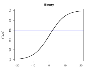
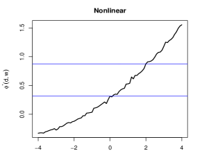
Figure 2: The curves correspond to the functions $\phi^{*}(d,w)$ in scenarios (i) and (ii) considered in this section for $w=(0,\dots,0,0.1)^{\intercal}\in\mathbb{R}^{7}$. The blue lines correspond to the true values for $d=-1$ and $d=2$ in each scenario and the difference between two blue lines is ${\rm CATE}(-1,2|w)$.

5.1 Binary outcome models

For $1\leq i\leq n$, the exposure $d_{i}$ is generated as $d_{i}=z_{i}^{\intercal}\gamma+v_{i}$ with $\gamma=c_{\gamma}\cdot(1,1,1,-1,-1,-1,-1)^{\intercal}$ and $v_{i}\sim N(0,1).$ We vary the IV strength such that $c_{\gamma}\in\{0.4,0.6,0.8\}$. We generate two distributions of the $z_{i}$: (1) $\{z_{i}\}_{1\leq i\leq n}$ are i.i.d. $N(0,{\rm I}_{p})$; (2) $\{z_{i}\}_{1\leq i\leq n}$ are i.i.d. uniformly distributed in $[-1.73,1.73].$ For the model (i), we generate $\{y_{i}\}_{1\leq i\leq n}$ via the mixed-logistic model

$$\mathbb{P}(y_{i}=1\mid d_{i},w_{i},u_{i})=\text{logit}\left(d_{i}\beta+w_{i}^{\intercal}\kappa+u_{i}\right)$$ (30)

with $\beta=0.25$, $\kappa=\eta=(0,0,0,0,0,0.4,0.2)^{\intercal}.$ The unmeasured confounder $u_{i}$ is generated as $u_{i}=0.25v_{i}+w_{i}^{\intercal}\eta+\xi_{i}$ with $\xi_{i}\sim N(0,1)$.

After integrating out $u_{i}$ conditioning on $v_{i},w_{i}$, the conditional distribution $y_{i}$ given $d_{i},w_{i}$ is in general not logistic. Conditioning on $w_{i}$, the unmeasured confounder $u_{i}$ is correlated with $v_{i}$ and $d_{i}$. The majority rule is satisfied: the first five IVs are valid and the last two are invalid. We construct 95% confidence intervals for ${\rm CATE}(-1,2|w)$ and compare our proposed SpotIV estimator with two other methods. The first one is the semi-parametric MLE assuming valid control function and valid IVs (Rothe, 2009), shorthanded as Valid-CF. Through this comparison, we can understand how invalid IVs affect the accuracy of the causal inference approaches by assuming valid IVs. The second one is the “Oracle” method, which is constructed with the prior knowledge of $\mathcal{V}$. It applies the Valid-CF by using the true valid IVs and treating the invalid IVs as known confounders. The oracle estimator is included as the benchmark. All the simulation results are calculated based on 500 replications.

In Table 1, we report the inference results for ${\rm CATE}(-1,2|w)$ for $w=(0,\dots,0,0.1)^{\intercal}\in\mathbb{R}^{7}$ in the binary outcome model (i). The proposed SpotIV achieves the desired 95% confidence level for Gaussian (Norm) and Uniform (Unif) $w_{i}$. The estimation errors get smaller with larger IV strengths and sample sizes. In contrast, the Valid-CF method has larger estimation errors, mainly due to the bias of using invalid IVs. The empirical coverage of the Valid-CF is lower than the nominal level across all settings. In terms of the empirical coverage, our proposed SpotIV is similar to the Oracle method, while SpotIV tends to have larger standard errors than the Oracle method. This happens since the SpotIV method identifies valid IVs in a data-dependent way. The “MT” column reports the proportion of simulations passing the majority rule test, detailed in Section 3.4. The majority rule is not rejected across most simulations. Our proposal is robust no matter whether the IVs are normal or uniform distributed.

			SpotIV				Valid-CF			Oracle
	$n$	$c_{\gamma}$	MAE	COV	SE	MT	MAE	COV	SE	MAE	COV	SE
Norm	500	0.4	0.115	0.922	0.14	1	0.205	0.552	0.11	0.077	0.914	0.12
	500	0.6	0.082	0.936	0.11	0.98	0.142	0.590	0.08	0.067	0.918	0.09
	500	0.8	0.070	0.968	0.10	1	0.130	0.592	0.07	0.055	0.932	0.08
	1000	0.4	0.073	0.918	0.10	1	0.204	0.380	0.09	0.055	0.928	0.08
	1000	0.6	0.056	0.920	0.08	1	0.160	0.298	0.06	0.044	0.944	0.07
	1000	0.8	0.046	0.960	0.08	0.99	0.131	0.330	0.05	0.040	0.940	0.06
Unif	500	0.4	0.112	0.940	0.14	1	0.195	0.638	0.12	0.064	0.966	0.11
	500	0.6	0.079	0.964	0.12	1	0.165	0.652	0.10	0.054	0.968	0.10
	500	0.8	0.067	0.968	0.10	1	0.125	0.752	0.11	0.054	0.984	0.09
	1000	0.4	0.082	0.918	0.11	1	0.199	0.442	0.09	0.046	0.958	0.08
	1000	0.6	0.052	0.952	0.09	0.99	0.164	0.458	0.08	0.042	0.962	0.07
	1000	0.8	0.052	0.972	0.08	0.99	0.126	0.616	0.08	0.040	0.986	0.07

Table 1: Inference for ${\rm CATE}(-1,2|w)$ in the binary outcome model (i). The “MAE”, “COV” and “SE” columns report the median absolute errors of $\widehat{\rm{CATE}}(-1,2|w)$, the empirical coverages of the confidence intervals and the average of estimated standard errors of the point estimators, respectively. The “MT” column reports the proportion of passing the majority rule testing in 500 replications. The columns indexed with “SpotIV” and “Valid-CF” correspond to the proposed method and the method assuming valid IVs, respectively. The columns indexed with “Oracle” correspond to the method which knows $\mathcal{V}$ as a priori.

The identifiability condition considered in Kolesár et al. (2015) and Bowden et al. (2015) requires the IV strength vector $\gamma$ and the invalidity form $\kappa+\eta$ to be nearly orthogonal in linear outcome models. Our configuration of $\gamma$, $\kappa$, and $\eta$ in setting (i) corresponds to the case where this orthogonality assumption fails to hold, and our proposal is reliable. In the online supplement, we explore settings where the orthogonality assumption is satisfied. Our proposal is reliable regardless of whether this assumption holds or not, which matches our theoretical results.

5.2 General nonlinear outcome models

We consider a nonlinear continuous outcome model as follows.

• Generate $\{y_{i}\}_{1\leq i\leq n}$ via $y_{i}=d_{i}\beta+z_{i}^{\intercal}\kappa+u_{i}+(d_{i}\beta+z_{i}^{\intercal}\kappa+u_{i})^{2}/3.$

The true parameters and the distribution of $u_{i}$ in (ii) are set to be the same as in (i) in Section 5.1.

We compare the SpotIV estimator with the two-stage hard-thresholding (TSHT) method (Guo et al., 2018), which is proposed to deal with possibly invalid IVs in linear outcome models. This comparison aims to understand the effect of mis-specifying a nonlinear model as linear. As reported in Table 2, the proposed SpotIV method has coverage probabilities close to 95% in model (ii). In comparison, the TSHT does not guarantee the 95% coverage and has larger estimation errors, mainly due to the fact that the TSHT method is only developed for linear outcome models.

			SpotIV				TSHT			Oracle
	$n$	$c_{\gamma}$	MAE	COV	SE	MT	MAE	COV	SE	MAE	COV	SE
Norm	500	0.4	0.084	0.932	0.12	1	1.693	0.040	0.27	0.058	0.960	0.09
	500	0.6	0.070	0.916	0.07	0.98	1.169	0.093	0.18	0.045	0.978	0.07
	500	0.8	0.055	0.928	0.08	1	0.865	0.110	0.13	0.046	0.972	0.07
	1000	0.4	0.059	0.910	0.09	1	1.535	0.107	0.21	0.045	0.920	0.06
	1000	0.6	0.046	0.938	0.07	1	0.399	0.363	0.13	0.036	0.952	0.05
	1000	0.8	0.037	0.950	0.06	1	0.268	0.383	0.10	0.030	0.966	0.05
Unif	500	0.4	0.289	0.910	0.44	1	0.847	0.093	0.13	0.200	0.949	0.36
	500	0.6	0.243	0.918	0.35	1	1.129	0.067	0.18	0.170	0.974	0.30
	500	0.8	0.187	0.936	0.30	1	0.847	0.093	0.13	0.147	0.952	0.28
	1000	0.4	0.199	0.892	0.30	1	0.583	0.140	0.20	0.138	0.944	0.25
	1000	0.6	0.147	0.948	0.23	1	0.323	0.133	0.05	0.113	0.956	0.21
	1000	0.8	0.130	0.938	0.21	1	0.267	0.423	0.10	0.106	0.956	0.18

Table 2: Inference for ${\rm CATE}(-1,2|w)$ in the nonlinear outcome model (ii). The “MAE”, “COV” and “SE” columns report the median absolute errors of $\widehat{\rm{CATE}}(-1,2|w)$, the empirical coverages of the confidence intervals and the average of estimated standard errors of the point estimators, respectively. The “MT” column reports the proportion of passing the majority rule testing in 500 replications. The columns indexed with “SpotIV” and “TSHT” correspond to the proposed method and the method in Guo et al. (2018), respectively. The columns indexed with “Oracle” correspond to the method which knows $\mathcal{V}$ as a priori.

5.3 Violation of majority rule

In this subsection, we examine the performance of our proposal when the majority rule is violated. Specifically, we consider the outcome model (i) with the two ways of violating the majority rule: (a) $\kappa=\eta=(0.4,0.4,0.4,0,0.4,0.4,0.4)^{\intercal}$; (b) $\kappa_{j}=\eta_{j}=\tilde{\xi}_{j}\cdot\gamma_{j}$ for $1\leq j\leq 7$ with $\tilde{\xi}_{j}\sim U[-1,1]$. The parameter $\gamma$ is the same as in Section 5.1. In (a), $\mathcal{V}=\{4\}$ and $\kappa_{j}/\gamma_{j}=\eta_{j}/\gamma_{j}=0.4$ for $j=1,2,3$ and $\kappa_{j}/\gamma_{j}=\eta_{j}/\gamma_{j}=-0.4$ for $j=5,6,7$. Hence, no IV should get four or more votes and the violation setting (a) is likely to be detected by the voting method detailed in Section 3.4. In (b), $\mathcal{V}=\emptyset$ and $\kappa_{j}/\gamma_{j}\sim U[-1,1]$ and hence no IV should get four or more votes. In the setting (b), $\kappa_{j}/\gamma_{j}$ is not as spread out as in (a) and hence our proposed voting method may be less powerful in comparison to the setting (a). In Table 3, we present the inference results under the configurations (a) and (b) with uniformly distributed IV measurements. In both settings, the SpotIV and Valid-CF have low coverages, which are as expected since the majority rule is violated. In setting (a), the violation of the majority rule is detected in most simulations. In setting (b), we cannot detect the violation of the majority rule in many cases. However, the detection gets easier as the IVs get stronger.

			SpotIV				Valid-CF
	$n$	$c_{\gamma}$	MAE	COV	SE	MT	MAE	COV	SE
(a)	1000	0.4	0.097	0.910	0.13	0.02	0.140	0.657	0.09
	1000	0.6	0.071	0.937	0.09	0.02	0.116	0.573	0.06
	1000	0.8	0.062	0.897	0.07	0.02	0.105	0.543	0.05
(b)	1000	0.4	0.136	0.743	0.11	0.80	0.104	0.708	0.08
	1000	0.6	0.140	0.567	0.09	0.71	0.091	0.644	0.06
	1000	0.8	0.137	0.523	0.07	0.66	0.083	0.610	0.05

Table 3: Inference for ${\rm CATE}(-1,2|w)$ in the binary outcome model (i) when the majority rule is violated. The columns indexed with “MAE”, “COV” and “SE” report the median absolute errors of $\widehat{\rm{CATE}}(-1,2|w)$, the empirical coverages of the confidence intervals and the average of estimated standard errors of the point estimators, respectively. The “MT” column reports the proportion of passing the majority rule testing in 500 replications. The columns indexed with “SpotIV” and “Valid-CF” correspond to the proposed method and the method assuming valid IVs, respectively.

6 Real data analysis

We apply the proposed SpotIV method to infer the causal effect of the income on the house owning through analyzing the data from China Family Panel Studies (Xie, 2012). The outcome $Y$ is a dichotomous variable indicating whether a family owns a house (1) or not (0). The exposure $D$ is the log-transformed family income per person as the income variable is highly right-skewed. The baseline covariates $X$ include the age, gender, and marriage status of the head of household. We include seven candidate IVs: the number of books at home, the education level of the head of the household, the registered residence type of the head of the household, monthly fees on dining, transport, travel, and health. In the preprocessing step, missing values are removed which gives a sample with the response ratio “own”: “not own”$\approx 5.88:1$. As the response ratio is highly unbalanced, we randomly remove part of the samples with positive response and arrive at a sample where “own”: “not own”$=2:1$. This gives a sample with 2538 observations. We choose these candidate IVs following a similar rationale as in the data analysis in Rothe (2009). Specifically, the first three candidate IVs are measures of human capital, which can be strongly related to income but have little effect on the housing decision. On the other hand, home ownership could be determined by the permanent components of the income stream. The expenses on different aspects (the last four candidate IVs) respond to the income (Campbell and Mankiw, 1991). Consumption in daily activities is a necessary part of life and always exists but do not decide on house investments. Therefore, the monthly consumptions are potentially valid IVs for the current study.

Applying the SpotIV method, the number of books at home and monthly fees on health are excluded from $\widehat{\mathcal{S}}$ and the remaining five IVs are selected as relevant IVs. Among these five IVs, the SpotIV method chooses the registered residence type of the head of the household, the monthly fees on transport, and the monthly fees on travel as valid IVs. The SpotIV method chooses the monthly fees on dining and monthly fees on health as invalid IVs.

In Figure 3, we report the inference results for the conditional average treatment effect for the male and female groups, respectively. Before adjusting for the endogeneity, income and house ownership tend to be negatively associated even though the relationship is insignificant. This result is not reliable due to the existence of unmeasured confounders. Assuming all IVs to be valid, the estimated causal effects are close to zero. This result can also be suspicious as two IVs are detected as invalid IVs based on the SpotIV method. Our proposed estimator leads to a significant and positive causal effect of income on house ownership. Comparing the fitted curves for the male and female groups, we observe an interesting phenomenon that the causal effects for males tend to be larger than those for females among subjects with a high or low income.

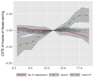
Figure 3: The $x$-axis denotes log-transformed income $(d_{1})$ and the $y$-axis denotes CATE($d_{1},10.2|w_{M}$) (left) and CATE($d_{1},10.2|w_{F}$) (right), where $w_{M}$ and $w_{F}$ are the average values of observed covariates for males and females respectively and the value 10.2 on the $x$-axis is the mean of log-transformed income in the sample. The solid lines are estimated without accounting for unmeasured confounders; the dot-dash lines are estimated based on the proposed SpotIV; the dashed lines are estimated assuming valid control functions (Condition 2.1). The shaded area corresponds to the point-wise 95% confidence intervals for each estimate.

Appendix A Proof of Lemma 4.1

Proposition A.1.

Under Condition 4.2, $\mathbb{E}[y_{i}|w_{i},v_{i}]=\mathbb{E}[y_{i}|w_{i}^{\intercal}\Theta,v_{i}]$.

Proof of Proposition A.1.

Let $\bar{\Sigma}=\mathbb{E}(w_{i}^{\intercal},v_{i})(w_{i}^{\intercal},v_{i})^{\intercal}]$, $\bar{\alpha}(y_{i})=\mathbb{E}[\bar{\Sigma}^{-1/2}(w_{i}^{\intercal},v_{i})|y_{i}]\in\mathbb{R}^{p+1}$, and $\bar{\Omega}=\textup{cov}(\bar{\alpha}(y_{i}))$. We first show that $\mathcal{L}(\bar{\Omega})\subseteq\mathcal{L}\left(\begin{pmatrix}\Theta^{*}&0\\ 0&1\end{pmatrix}\right)$. Next, we show

$$\mathcal{L}(\bar{\Omega}_{1:p,1:p})=\mathcal{L}(\Omega)=\mathcal{L}\left(\Theta^{*}\right).$$ (31)

We know that for binary outcomes,

$$\mathbb{E}[y_{i}|w_{i},v_{i}]=\mathbb{P}(y_{i}=1|w_{i},v_{i})=\mathbb{P}(y_{i}=1|w_{i}^{\intercal}\Theta^{*},v_{i}).$$

That is, $y_{i}\perp(w_{i},v_{i})|(w_{i}^{\intercal}\Theta^{*},v_{i})$. By Condition 4.2, $\mathbb{E}[(w_{i}^{\intercal},v_{i})|w_{i}^{\intercal}\Theta^{*},v_{i}]$ is linear in $w_{i}^{\intercal}\Theta^{*},v_{i}$. Therefore, by Theorem 3.1 in Li (1991), we know that $\mathcal{L}(\bar{\Omega})\subseteq\mathcal{L}\left(\begin{pmatrix}\Theta^{*}&0\\ 0&1\end{pmatrix}\right)$.

Next, we show (31). The first equality holds because $\mathbb{E}[w_{i}^{\intercal}v_{i}]=0$ by (4). As $\mathcal{L}(\bar{\Omega})\subseteq\mathcal{L}\left(\begin{pmatrix}\Theta^{*}&0\\ 0&1\end{pmatrix}\right)$, we know

$$\bar{\Omega}=\begin{pmatrix}\Theta^{*}&0\\ 0&1\end{pmatrix}\begin{pmatrix}R_{1,1}&R_{1,2}\\ R_{2,1}&R_{2,2}\end{pmatrix}$$ (32)

for some constant matrix $R\in\mathbb{R}^{(p_{\eta}+2)\times(p+1)}$ and $R_{1,1}\in\mathbb{R}^{(p_{\eta}+1)\times p}$. We arrive at $\bar{\Omega}_{1:p,1:p}=\Theta^{*}R_{1,1}$. As rank$(\bar{\Omega}_{1:p,1:p})=M=p_{\eta}+1=$rank$(\Theta^{*})$, the proof of (31) is complete now.

∎

Proposition A.2 (Convergence rate of $\widehat{\Theta}$).

Under the conditions of Lemma 4.1, we have

$$\mathbb{P}\left(\max_{1\leq m\leq M}\|\widehat{\Theta}_{.,m}-\Theta_{.,m}\|_{2}\geq C_{1}\sqrt{\frac{t}{n}}\right)\leq\exp(-C_{2}t).$$

Proof of PropositionA.2.

Notice that

$$\Omega=\Sigma^{-1/2}Cov(\alpha(y_{i}))\Sigma^{-1/2}=\Sigma^{-1/2}\mathbb{E}[\alpha(y_{i})\alpha(y_{i})^{\intercal}]\Sigma^{-1/2}$$

as $\mathbb{E}[\alpha(y_{i})]=\mathbb{E}[w_{i}]=0$.

The following decomposition holds

$$\|\widehat{\Omega}-\Omega\|_{2} \leq 2\|\Sigma^{-1/2}-\widehat{\Sigma}^{-1/2}\|_{2}\|cov(\alpha(y_{i}))\Sigma^{-1/2}\|_{2}$$

$$\quad+\|\Sigma^{-1/2}\|^{2}_{2}\|cov(\alpha(y_{i}))-\frac{1}{n}\sum_{i=1}^{n}\hat{\alpha}(y_{i})\hat{\alpha}(y_{i})^{\intercal}\|_{2}+r_{n},$$ (33)

where $r_{n}$ is of smaller order than the first two terms.

For the first term,

$$\|\Sigma^{-1/2}-\widehat{\Sigma}^{-1/2}\|_{2}\leq\|\Sigma-\widehat{\Sigma}\|_{2}\|\Sigma^{1/2}+\widehat{\Sigma}^{1/2}\|^{-1}_{2}.$$

Since $\widehat{\Sigma}$ is an average of i.i.d. sub-exponential variables, we have

$$\mathbb{P}\left(\|\Sigma-\widehat{\Sigma}\|_{2}\geq c\sqrt{t/n}\right)\leq\exp(-ct).$$

As $\|\Sigma^{-1/2}cov(\alpha(y_{i}))\|_{2}\leq C<\infty$, for the first term in (A),

$$\mathbb{P}\left(2\|\Sigma^{-1/2}-\widehat{\Sigma}^{-1/2}\|_{2}\|cov(\alpha(y_{i}))\Sigma^{-1/2}\|_{2}\geq c_{1}\sqrt{t/n}\right)\leq\exp(-c_{2}t).$$ (34)

To bound the second term in (A), for binary $y_{i}$, it holds that

$$\alpha(1)=\mathbb{E}[w_{i}|y_{i}=1]~{}~{}\hat{\alpha}(1)=\frac{1}{\sum_{i=1}^{n}\mathbbm{1}(y_{i}=0)}\sum_{i=1}^{n}w_{i}\mathbbm{1}(y_{i}=1)$$

$$\alpha(0)=\mathbb{E}[w_{i}|y_{i}=0]~{}~{}\hat{\alpha}(0)=\frac{1}{\sum_{i=1}^{n}\mathbbm{1}(y_{i}=0)}\sum_{i=1}^{n}w_{i}\mathbbm{1}(y_{i}=0).$$

By some simple algebra, we can show that

$$cov(\alpha(y_{i}))=\mathbb{P}(y_{i}=1)\mathbb{P}(y_{i}=0)(\alpha(1)-\alpha(0))(\alpha(1)-\alpha(0))^{\intercal}.$$

The following decomposition holds

$$\left\|\frac{1}{n}\sum_{i=1}^{n}\hat{\alpha}(y_{i})\hat{\alpha}(y_{i})^{\intercal}-\frac{cov(\alpha(y_{i}))}{\mathbb{P}(y_{i}=1)\mathbb{P}(y_{i}=0)}\right\|_{2}$$

$$\leq 2\|(\hat{\alpha}(1)-\hat{\alpha}(0)-\alpha(1)+\alpha(0))(\alpha(1)-\alpha(0))^{\intercal}\|_{2}+\|\alpha(1)-\alpha(0)-\hat{\alpha}(1)+\hat{\alpha}(0)\|_{2}^{2}$$

$$\leq 4\|\alpha(1)-\alpha(0)\|_{2}\max_{k\in\{0,1\}}\|\hat{\alpha}(k)-\alpha(k)\|_{2}+4\max_{k\in\{0,1\}}\|\hat{\alpha}(k)-\alpha(k)\|_{2}^{2}.$$

First notice that $\alpha(k)=\frac{\mathbb{E}\left[w_{i}\mathbbm{1}(y_{i}=k)\right]}{\mathbb{P}(y_{i}=k)}$. Therefore,

$$\|\hat{\alpha}(k)-\alpha(k)\|_{2} \leq|\frac{1}{\mathbb{P}(y_{i}=k)}-\frac{n}{\sum_{i=1}^{n}\mathbbm{1}(y_{i}=k)}|\|\mathbb{E}\left[w^{\intercal}_{i}\mathbbm{1}(y_{i}=k)\right]\|_{2}$$

$$+\frac{1}{\mathbb{P}(y_{i}=k)}\|\frac{1}{n}\sum_{i=1}^{n}w_{i}\mathbbm{1}(y_{i}=k)-\mathbb{E}\left[w_{i}\mathbbm{1}(y_{i}=k)\right]\|_{2}.$$

$$|\frac{1}{n}\sum_{i=1}^{n}(\hat{v}_{i}-v_{i})\mathbbm{1}(y_{i}=k)| =|\frac{1}{n}\sum_{i=1}^{n}\mathbbm{1}(y_{i}=k)w_{i}^{\intercal}(\hat{\gamma}-\gamma)|$$

$$\leq\|\frac{1}{n}\sum_{i=1}^{n}\mathbbm{1}(y_{i}=k)w_{i}^{\intercal}\|_{2}\|\hat{\gamma}-\gamma\|_{2}.$$

Hence, it is straight forward to show that

$$\mathbb{P}\left(\left\|\frac{1}{n}\sum_{i=1}^{n}\hat{\alpha}(y_{i})\hat{\alpha}(y_{i})^{\intercal}-\frac{cov(\alpha(y_{i}))}{\mathbb{P}(y_{i}=1)\mathbb{P}(y_{i}=0)}\right\|_{2}\geq c_{3}\sqrt{t/n}\right)\leq\exp(-c_{4}t)$$

for sufficiently large constants $c_{3}$ and $c_{4}$.

In view of (A), we have shown

$$\mathbb{P}\left(\|\widehat{\Omega}-\Omega\|_{2}\geq c_{5}\sqrt{\frac{t}{n}}\right)\leq\exp(-c_{6}t)$$ (35)

for sufficiently large constants $c_{5}$ and $c_{6}$.

Next, we show the the eigenvalues of $\widehat{\Omega}$ converge to the eigenvalues of $\Omega$. In fact,

$$\max_{1\leq k\leq p}\left|\hat{\lambda}_{k}-\hat{\lambda}_{k}\right|\leq\max_{\|u\|_{2}=1}|u^{\intercal}(\widehat{\Omega}-\Omega)u|\leq\|\widehat{\Omega}-\Omega\|_{2}.$$

For the eigenvectors, we use Theorem 5 of Karoui (2008). Under Condition 4.2, we have

$$\|\widehat{\Phi}_{.,m}-\Phi_{.,m}\|_{2}\leq\frac{\|\widehat{\Omega}-\Omega\|_{2}}{\lambda_{m}(\Omega)}~{}~{}\forall~{}1\leq m\leq 2.$$

In view of (35), we have shown

$$\mathbb{P}\left(\max_{1\leq m\leq M}\|\widehat{\Theta}_{.,m}-\Theta_{.,m}\|_{2}\geq C_{1}\sqrt{\frac{t}{n}}\right)\leq\exp(-C_{2}t).$$

∎

Proof of Lemma 4.1.

For $\widehat{\gamma}$ computed via (18), under Condition 4.1, it is easy to show that

$$\sqrt{n}(\hat{\gamma}-\gamma)\xrightarrow{D}N\left(0,\sigma^{2}_{v}\mathbb{E}^{-1}[w_{i}w_{i}^{\intercal}]\right).$$ (36)

Define an event

$$E_{1}=\left\{\widehat{M}=M,\widehat{\mathcal{S}}=\mathcal{S}\right\}.$$ (37)

We first show that $\mathbb{P}(E_{1})\rightarrow 1$ as $n\rightarrow\infty$. Given the results of Proposition A.2, by Theorem 2 of Zhu et al. (2006), we know that for $C_{n}=n^{c_{0}}$ and $c_{0}\in(0,1)$, $\mathbb{P}(\widehat{M}=M)\rightarrow 1$.

For the last statement in $E_{1}$, it is easy to show

$$|\hat{\sigma}_{v}^{2}-\sigma_{v}^{2}|=O_{P}(n^{-1/2}).$$

Let $\widehat{\omega}_{j}=\hat{\sigma}^{2}_{v}\{\widehat{\Sigma}^{-1}\}_{j,j}$. For $j\in\mathcal{S}$, we have

$$\mathbb{P}\left(\left|\widehat{\gamma}_{j}\right|\geq\sqrt{\widehat{\omega}_{j}}\sqrt{\frac{2.01\log n}{n}}\right)\geq\mathbb{P}\left(|\gamma_{j}|-\left|\widehat{\gamma}_{j}-\gamma_{j}\right|\geq\sqrt{\widehat{\omega}_{j}}\sqrt{\frac{2.01\log n}{n}}\right)$$

$$=\mathbb{P}\left(\left|\widehat{\gamma}_{j}-\gamma_{j}\right|\leq|\gamma_{j}|-\sqrt{\widehat{\omega}_{j}}\sqrt{\frac{2.01\log n}{n}}\right)\rightarrow 1,$$

where the convergence follows from (36) and $|\gamma_{j}|\geq c_{0}>0$ for $j\in\mathcal{S}$. For $j\in\mathcal{S}^{c}$, we have

$$\mathbb{P}\left(\left|\widehat{\gamma}_{j}\right|>\sqrt{\widehat{\omega}_{j}}\sqrt{\frac{2.01\log n}{n}}\right)=\mathbb{P}\left(\left|\widehat{\gamma}_{j}-\gamma_{j}\right|>\sqrt{\widehat{\omega}_{j}}\sqrt{\frac{2.01\log n}{n}}\right)=o(1),$$

where the last step is due to $\|\hat{\gamma}-\gamma\|_{2}=O_{P}(n^{-1/2})$. Combining above two expressions, we have establish that

$$\mathbf{P}\left(\widehat{\mathcal{S}}=\mathcal{S}\right)\rightarrow 1.$$ (38)

It suffices to prove the rest of the results conditioning on the event $E_{1}$. Under the majority rule, the median of $\{\widehat{\Theta}_{j,m}/\hat{\gamma}_{j}\}_{j\in S}$ must be evaluated at a valid IV for $m=1,\dots,M$.

Together with Proposition A.2, we have

$$\mathbb{P}\left(\max_{1\leq m\leq M}\max_{j\in\mathcal{S}}\left|\frac{\widehat{\Theta}_{j,m}}{\hat{\gamma}_{j}}-\frac{\Theta_{j,m}}{\gamma_{j}}\right|\geq c_{1}\sqrt{\frac{t}{n}}\right)\leq\exp(-c_{2}t)$$ (39)

for some positive constants $c_{1}$ and $c_{2}$. Notice that

$$\max_{1\leq m\leq M}|\hat{b}_{m}-b_{m}|\leq\max_{1\leq m\leq M}\max_{j\in\mathcal{S}}\left|\frac{\widehat{\Theta}_{j,m}}{\hat{\gamma}_{j}}-\frac{\Theta_{j,m}}{\gamma_{j}}\right|.$$

The proof for (28) is complete now.

Finally, we are left to show $\mathbb{E}[y_{i}|d_{i},w_{i}^{\intercal},v_{i}]=\mathbb{E}[y_{i}|(d_{i},w_{i}^{\intercal})B,v_{i}]$. To see this, notice that by Condition 4.2,

$$\mathbb{E}[y_{i}|w_{i},v_{i}]=\mathbb{E}[y_{i}|w_{i}^{\intercal}\Theta^{*},v_{i}]=\mathbb{E}[y_{i}|w_{i}^{\intercal}\Theta,v_{i}].$$

As $\Theta$ has the smallest possible dimension, we know $\Theta=\Theta^{*}T$ for some constant matrix $T\in\mathbb{R}^{p_{\eta}+1}\times M$. Therefore,

$$\mathbb{E}[y_{i}|d_{i},w_{i},v_{i}] =\mathbb{E}[y_{i}|w_{i},v_{i}]=\mathbb{E}[y_{i}|w_{i}^{\intercal}\Theta,v_{i}]=\mathbb{E}[y_{i}|w_{i}^{\intercal}\Theta^{*}T,v_{i}]$$

$$=\mathbb{E}[y_{i}|(d_{i}-v_{i},w_{i}^{\intercal})B^{*}T,v_{i}]$$

$$=\mathbb{E}[y_{i}|(d_{i},w_{i}^{\intercal})B^{*}T,v_{i}]$$

To complete the proof, we only need to show $B$ defined in (27) satisfies that $B=B^{*}T$ given that $\Theta=\Theta^{*}T$ for some invertible $T\in\mathbb{R}^{(p_{\eta}+1)\times(p_{\eta}+1)}$ by (32). Notice that $\Theta_{j,.}=\Theta^{*}_{j,.}T$. If $j\in V$, then $\Theta_{j,.}=(\gamma_{j}\beta,\bm{0}_{p_{\eta}}^{\intercal})T$ and $\Theta_{j,.}/\gamma_{j}=(\beta,\bm{0}_{p_{\eta}}^{\intercal})T$. Therefore, $b_{k}=Median(\{\Theta_{j,k}/\gamma_{j}\}_{j\in\mathcal{S}})=(\beta,\bm{0}_{p_{\eta}}^{\intercal})T_{.,k}$ for $k=1,\dots,M$. Moreover,

$$\Theta_{.,k}-b_{k}\gamma=(\gamma\beta+\kappa,\eta)T_{.,k}-(\beta\gamma,\bm{0}_{p_{\eta}}^{\intercal})T_{.,k}=(\kappa,\eta)T_{.,k},~{}k=1,\dots,M.$$

Hence, we have showed that $B=B^{*}T$. ∎

Appendix B Proof of Theorem 4.1

It follows from the condition $h=n^{-c}$ for $0<c<1/4$ that $nh^{4}\gg\log n$ and $h\log n\rightarrow 0.$ We recall the following definitions,

$$t_{i}=((d_{i},w_{i}^{\intercal})B,{v}_{i})^{\intercal},\quad\widehat{t}_{i}=((d_{i},w_{i}^{\intercal})\widehat{B},\widehat{v}_{i})^{\intercal},\quad{s}_{i}=((d,w^{\intercal})B,{v}_{i})^{\intercal},\quad\widehat{s}_{i}=((d,w^{\intercal})\widehat{B},\widehat{v}_{i})^{\intercal}.$$

In event $E_{1}$ (37), $\{\widehat{M}=M=2\}$ and the kernel is defined in three dimensions. That is, for $a,b\in\mathbb{R}^{3},$

$$K_{H}(a,b)=\prod_{l=1}^{3}\frac{1}{h}k\left(\frac{a_{l}-b_{l}}{h}\right),$$

where $h$ is the bandwidth and $k(x)={\bf 1}\left(|x|\leq 1/2\right).$ We define the events

$$\mathcal{A}_{1}=\left\{\|\widehat{B}-B\|_{2}\leq C\sqrt{\frac{\log n}{n}},\|\widehat{\gamma}-\gamma\|_{2}\leq C\sqrt{\frac{\log n}{n}}\right\},~{}~{}\mathcal{A}_{2}=\max\{\|w_{i}\|_{\infty},|d_{i}|\}\lesssim\sqrt{\log n}.$$

By Lemma 4.1 and $w_{i}$ and $v_{i}$ being sub-gaussian, we establish that $\mathbf{P}(\mathcal{A}_{1}\cap\mathcal{A}_{3})\geq{1-n^{-c}}-P(E_{1})$. On the event $\mathcal{A}_{1}\cap\mathcal{A}_{2},$ we have

$$\max_{1\leq i\leq n}\max\left\{\|\widehat{s}_{i}-s_{i}\|_{2},\|\widehat{t}_{i}-t_{i}\|_{2}\right\}\leq C{{\log n}}/{\sqrt{n}}$$

for a large positive constant $C>0.$

We start with the decomposition

$$\widehat{\phi}(d,w)-{\phi}^{*}(d,w)=\frac{1}{n}\sum_{i=1}^{n}\left[\widehat{g}(\widehat{s}_{i})-{g}(\widehat{s}_{i})\right]+\frac{1}{n}\sum_{i=1}^{n}{g}(\widehat{s}_{i})-\int{g}({s}_{i})f_{v}(v_{i})dv_{i}$$ (40)

where $f_{v}$ is the density of $v_{i}.$ By Lemma 4.1, we define

$$\epsilon_{i}=y_{i}-\mathbb{E}[y_{i}|(d_{i},w^{\intercal}_{i})B,v_{i}]=y_{i}-g((d_{i},w_{i}^{\intercal})B,v_{i})\quad\text{for}\;1\leq i\leq n.$$ (41)

We plug in the expression of $\widehat{g}(\widehat{s}_{i})$ and decompose the error $\frac{1}{n}\sum_{i=1}^{n}\left[\widehat{g}(\widehat{s}_{i})-{g}(\widehat{s}_{i})\right]$ as

$$\frac{1}{n}\sum_{i=1}^{n}\frac{\sum_{j=1}^{n}[y_{j}-{g}(\widehat{s}_{i})]K_{H}(\widehat{s}_{i},\widehat{t}_{j})}{\sum_{j=1}^{n}K_{H}(\widehat{s}_{i},\widehat{t}_{j})}=\frac{1}{n}\sum_{i=1}^{n}\frac{\sum_{j=1}^{n}\epsilon_{j}K_{H}(\widehat{s}_{i},\widehat{t}_{j})}{\sum_{j=1}^{n}K_{H}(\widehat{s}_{i},\widehat{t}_{j})}$$ (42)

$$+\frac{1}{n}\sum_{i=1}^{n}\frac{\sum_{j=1}^{n}[g(\widehat{t}_{j})-{g}(\widehat{s}_{i})]K_{H}(\widehat{s}_{i},\widehat{t}_{j})}{\sum_{j=1}^{n}K_{H}(\widehat{s}_{i},\widehat{t}_{j})}+\frac{1}{n}\sum_{i=1}^{n}\frac{\sum_{j=1}^{n}[g({t}_{j})-{g}(\widehat{t}_{j})]K_{H}(\widehat{s}_{i},\widehat{t}_{j})}{\sum_{j=1}^{n}K_{H}(\widehat{s}_{i},\widehat{t}_{j})}.$$

Since

$$\left|{g}(\widehat{t}_{j})-g({t}_{j})\right|\cdot K_{H}(\widehat{s}_{i},\widehat{t}_{j})\leq\|\triangledown g({t}_{j}+c(\widehat{t}_{j}-{t}_{j}))\|_{2}\|\widehat{t}_{j}-{t}_{j}\|_{2}\cdot K_{H}(\widehat{s}_{i},\widehat{t}_{j}),$$

we apply the boundedness assumption on $\triangledown g$ imposed in Condition 5.3 (b) and obtain that $\left|{g}(\widehat{t}_{j})-g({t}_{j})\right|\lesssim\log n/\sqrt{n}$ on the event $\mathcal{A}.$ Here, we use the fact that, if $K_{H}(\widehat{s}_{i},\widehat{t}_{j})>0$ and $C\log n/\sqrt{n}\leq h/2,$ then $\|\widehat{t}_{j}-s_{i}\|_{\infty}\leq\|\widehat{t}_{j}-\widehat{s}_{i}\|_{\infty}+\|\widehat{s}_{i}-s_{i}\|_{\infty}\leq h.$

Hence, we have

$$\left|\frac{1}{n}\sum_{i=1}^{n}\frac{\sum_{j=1}^{n}[g({t}_{j})-{g}(\widehat{t}_{j})]K_{H}(\widehat{s}_{i},\widehat{t}_{j})}{\sum_{j=1}^{n}K_{H}(\widehat{s}_{i},\widehat{t}_{j})}\right|\lesssim{\log n}/\sqrt{{n}}.$$

Then following from (40) and (42), it is sufficient to control the following terms,

$$\small\underbrace{\frac{1}{n}\sum_{i=1}^{n}{g}(\widehat{s}_{i})-\int{g}({s}_{i})f_{v}(v_{i})dv_{i}}_{T_{1}}+\underbrace{\frac{1}{n}\sum_{i=1}^{n}\frac{\sum_{j=1}^{n}\epsilon_{j}K_{H}(\widehat{s}_{i},\widehat{t}_{j})}{\sum_{j=1}^{n}K_{H}(\widehat{s}_{i},\widehat{t}_{j})}}_{T_{2}}+\underbrace{\frac{1}{n}\sum_{i=1}^{n}\frac{\sum_{j=1}^{n}[g(\widehat{t}_{j})-{g}(\widehat{s}_{i})]K_{H}(\widehat{s}_{i},\widehat{t}_{j})}{\sum_{j=1}^{n}K_{H}(\widehat{s}_{i},\widehat{t}_{j})}}_{T_{3}}.$$ (43)

We now control the three terms $T_{1},T_{2}$ and $T_{3}$ separately.

Control of $T_{1}$.

The term $T_{1}$ is controlled by the following lemma, whose proof is presented in Section C.1.

Lemma B.1.

Suppose the assumptions of Theorem 4.1 hold, then with probability larger than $1-n^{-c}-\frac{1}{t^{2}},$

$$\left|\frac{1}{n}\sum_{i=1}^{n}{g}(\widehat{s}_{i})-\int{g}({s}_{i})f_{v}(v_{i})dv_{i}\right|\lesssim{\frac{t+\log n}{\sqrt{n}}}$$ (44)

Control of $T_{2}$.

We approximate $T_{2}$ by $\frac{1}{n}\sum_{i=1}^{n}\frac{\frac{1}{n}\sum_{j=1}^{n}\epsilon_{j}K_{H}({s}_{i},{t}_{j})}{\frac{1}{n}\sum_{j=1}^{n}K_{H}({s}_{i},{t}_{j})}=\frac{1}{n}\sum_{j=1}^{n}\epsilon_{j}a_{j}$ with

$$a_{j}=\frac{1}{n}\sum_{i=1}^{n}\frac{K_{H}({s}_{i},{t}_{j})}{\frac{1}{n}\sum_{j=1}^{n}K_{H}({s}_{i},{t}_{j})}.$$ (45)

Then the approximation error is

$$\frac{1}{n}\sum_{i=1}^{n}\frac{\frac{1}{n}\sum_{j=1}^{n}\epsilon_{j}K_{H}(\widehat{s}_{i},\widehat{t}_{j})}{\frac{1}{n}\sum_{j=1}^{n}K_{H}(\widehat{s}_{i},\widehat{t}_{j})}-\frac{1}{n}\sum_{i=1}^{n}\frac{\frac{1}{n}\sum_{j=1}^{n}\epsilon_{j}K_{H}({s}_{i},{t}_{j})}{\frac{1}{n}\sum_{j=1}^{n}K_{H}({s}_{i},{t}_{j})}$$ (46)

$$= \frac{1}{n}\sum_{i=1}^{n}\frac{\frac{1}{n}\sum_{j=1}^{n}\epsilon_{j}[K_{H}(\widehat{s}_{i},\widehat{t}_{j})-K_{H}(s_{i},{t}_{j})]}{\frac{1}{n}\sum_{j=1}^{n}K_{H}(\widehat{s}_{i},\widehat{t}_{j})}+\frac{1}{n}\sum_{i=1}^{n}\frac{\frac{1}{n}\sum_{j=1}^{n}\epsilon_{j}K_{H}({s}_{i},{t}_{j})}{\frac{1}{n}\sum_{j=1}^{n}K_{H}({s}_{i},{t}_{j})}\left(\frac{\frac{1}{n}\sum_{j=1}^{n}K_{H}({s}_{i},{t}_{j})}{\frac{1}{n}\sum_{j=1}^{n}K_{H}(\widehat{s}_{i},\widehat{t}_{j})}-1\right)$$

The following two lemmas are needed to control $T_{2}$. The proofs of Lemma B.2 and 52 are presented in Section C.2 and C.3, respectively.

Lemma B.2.

Suppose the assumptions of Theorem 4.1 hold, then with probability larger than $1-n^{-C}$ for some positive constant $C>1$, for all $1\leq i\leq n,$

$$\frac{1}{2}f_{t}(s_{i})-C\sqrt{f_{t}(s_{i})\frac{\log n}{nh^{3}}}\leq\frac{1}{n}\sum_{j=1}^{n}K_{H}({s}_{i},{t}_{j})\leq f_{t}(s_{i})+C\sqrt{f_{t}(s_{i})\frac{\log n}{nh^{3}}}$$ (47)

$$\frac{1}{n}\sum_{j=1}^{n}\left|K_{H}({s}_{i},{t}_{j})-K_{H}(\widehat{s}_{i},\widehat{t}_{j})\right|\lesssim\frac{\log n}{\sqrt{n}h}$$ (48)

$$\left|\frac{1}{n}\sum_{j=1}^{n}\epsilon_{j}K_{H}({s}_{i},{t}_{j})\right|\lesssim\sqrt{\frac{\log n}{nh^{3}}}$$ (49)

$$\left|\frac{1}{n}\sum_{j=1}^{n}\epsilon_{j}[K_{H}(\widehat{s}_{i},\widehat{t}_{j})-K_{H}(s_{i},{t}_{j})]\right|\lesssim\frac{\log n}{n^{3/4}h^{2}}.$$ (50)

Lemma B.3.

Suppose the assumptions of Theorem 4.1 hold, then

$$\frac{\frac{1}{n}\sum_{j=1}^{n}\epsilon_{j}a_{j}}{\sqrt{\frac{1}{n^{2}}\sum_{j=1}^{n}{\rm Var}(\epsilon_{j}\mid d_{j},w_{j})a^{2}_{j}}}\rightarrow N(0,1)$$ (51)

where $\epsilon_{j}$ is defined in (41) and $a_{j}$ is defined in (45). With probability larger than $1-n^{-C},$

$$\sqrt{\frac{1}{n^{2}}\sum_{j=1}^{n}{\rm Var}(\epsilon_{j}\mid d_{j},w_{j})a^{2}_{j}}\asymp\frac{1}{\sqrt{nh^{2}}}$$ (52)

A combination of (47) and (48) leads to

$$\frac{1}{8}f_{t}(s_{i})-C\sqrt{\left|f_{t}(s_{i})\right|\frac{\log n}{nh^{3}}}\leq\frac{1}{n}\sum_{j=1}^{n}K_{H}(\widehat{s}_{i},\widehat{t}_{j})\leq f_{t}(s_{i})+C\sqrt{\left|f_{t}(s_{i})\right|\frac{\log n}{nh^{3}}}.$$ (53)

Together with (47), (48), (49) and $\min_{i}f_{t}(s_{i})\geq c_{0}$ for some positive constant $c_{0}>0,$

$$\mathbf{P}\left(\left|\frac{1}{n}\sum_{i=1}^{n}\frac{\frac{1}{n}\sum_{j=1}^{n}\epsilon_{j}K_{H}({s}_{i},{t}_{j})}{\frac{1}{n}\sum_{j=1}^{n}K_{H}({s}_{i},{t}_{j})}\left(\frac{\frac{1}{n}\sum_{j=1}^{n}K_{H}({s}_{i},{t}_{j})}{\frac{1}{n}\sum_{j=1}^{n}K_{H}(\widehat{s}_{i},\widehat{t}_{j})}-1\right)\right|\gtrsim\frac{(\log n)^{3/2}}{nh^{5/2}}\right)\leq n^{-C}$$

By (53), (50) and $\min_{i}f_{t}(s_{i})\geq c_{0},$ we have

$$\mathbf{P}\left(\left|\frac{1}{n}\sum_{i=1}^{n}\frac{\frac{1}{n}\sum_{j=1}^{n}\epsilon_{j}[K_{H}(\widehat{s}_{i},\widehat{t}_{j})-K_{H}(s_{i},{t}_{j})]}{\frac{1}{n}\sum_{j=1}^{n}K_{H}(\widehat{s}_{i},\widehat{t}_{j})}\right|\gtrsim\frac{\log n}{n^{3/4}h^{2}}\right)\leq n^{-C}.$$

Since $nh^{4}\gg(\log n)^{2},$ we have

$$\sqrt{nh^{2}}\left|\frac{1}{n}\sum_{i=1}^{n}\frac{\frac{1}{n}\sum_{j=1}^{n}\epsilon_{j}K_{H}(\widehat{s}_{i},\widehat{t}_{j})}{\frac{1}{n}\sum_{j=1}^{n}K_{H}(\widehat{s}_{i},\widehat{t}_{j})}-\frac{1}{n}\sum_{i=1}^{n}\frac{\frac{1}{n}\sum_{j=1}^{n}\epsilon_{j}K_{H}({s}_{i},{t}_{j})}{\frac{1}{n}\sum_{j=1}^{n}K_{H}({s}_{i},{t}_{j})}\right|=o_{p}(1).$$

Together with Lemma 52, we establish that

$$\frac{\frac{1}{n}\sum_{i=1}^{n}\frac{\frac{1}{n}\sum_{j=1}^{n}\epsilon_{j}K_{H}(\widehat{s}_{i},\widehat{t}_{j})}{\frac{1}{n}\sum_{j=1}^{n}K_{H}(\widehat{s}_{i},\widehat{t}_{j})}}{\sqrt{\frac{1}{n^{2}}\sum_{j=1}^{n}{\rm Var}(\epsilon_{j})a^{2}_{j}}}\rightarrow N(0,1).$$ (54)

Control of $T_{3}$.

We decompose $T_{3}$ as

$$\frac{1}{n}\sum_{i=1}^{n}\frac{\sum_{j=1}^{n}[{\triangledown g}(\widehat{s}_{i})]^{\intercal}(\widehat{t}_{j}-\widehat{s}_{i})K_{H}(\widehat{s}_{i},\widehat{t}_{j})}{\sum_{j=1}^{n}K_{H}(\widehat{s}_{i},\widehat{t}_{j})}+\frac{1}{n}\sum_{i=1}^{n}\frac{\sum_{j=1}^{n}(\widehat{t}_{j}-\widehat{s}_{i})^{\intercal}\triangle g(\widehat{s}_{i}+c_{ij}(\widehat{t}_{j}-\widehat{s}_{i}))(\widehat{t}_{j}-\widehat{s}_{i})K_{H}(\widehat{s}_{i},\widehat{t}_{j})}{\sum_{j=1}^{n}K_{H}(\widehat{s}_{i},\widehat{t}_{j})}$$ (55)

for some constant $c_{ij}\in(0,1).$ We show that the second term of (55) is the higher order term, controlled as,

$$\left|\frac{1}{n}\sum_{i=1}^{n}\frac{\sum_{j=1}^{n}(\widehat{t}_{j}-\widehat{s}_{i})^{\intercal}\triangle g(\widehat{s}_{i}+c(\widehat{t}_{j}-\widehat{s}_{i}))(\widehat{t}_{j}-\widehat{s}_{i})K_{H}(\widehat{s}_{i},\widehat{t}_{j})}{\sum_{j=1}^{n}K_{H}(\widehat{s}_{i},\widehat{t}_{j})}\right|\leq h^{2}$$

To establish the above inequality, we apply the boundedness assumption on the hessian $\triangle g$ imposed in Condition 5.3 (b) and and we use the fact that, if $K_{H}(\widehat{s}_{i},\widehat{t}_{j})>0$ and $C\log n/\sqrt{n}\leq h/2,$ then $\|\widehat{t}_{j}-s_{i}\|_{\infty}\leq\|\widehat{t}_{j}-\widehat{s}_{i}\|_{\infty}+\|\widehat{s}_{i}-s_{i}\|_{\infty}\leq h.$

Now we control the first term of (55) as

$$\frac{1}{n}\sum_{i=1}^{n}\frac{\sum_{j=1}^{n}[{\triangledown g}(\widehat{s}_{i})]^{\intercal}(\widehat{t}_{j}-\widehat{s}_{i})K_{H}(\widehat{s}_{i},\widehat{t}_{j})}{\sum_{j=1}^{n}K_{H}(\widehat{s}_{i},\widehat{t}_{j})}$$ (56)

$$=\frac{1}{n}\sum_{i=1}^{n}\frac{\sum_{j\neq i}[{\triangledown g}(\widehat{s}_{i})]^{\intercal}(\widehat{t}_{j}-\widehat{s}_{i})K_{H}(\widehat{s}_{i},\widehat{t}_{j})}{\sum_{j=1}^{n}K_{H}(\widehat{s}_{i},\widehat{t}_{j})}+\frac{1}{n}\sum_{i=1}^{n}\frac{[{\triangledown g}(\widehat{s}_{i})]^{\intercal}(\widehat{t}_{i}-\widehat{s}_{i})K_{H}(\widehat{s}_{i},\widehat{t}_{i})}{\sum_{j=1}^{n}K_{H}(\widehat{s}_{i},\widehat{t}_{j})}$$

$$=\frac{1}{n}\sum_{i=1}^{n}\frac{\sum_{j\neq i}[{\triangledown g}({s}_{i})]^{\intercal}({t}_{j}-{s}_{i})K_{H}({s}_{i},{t}_{j})}{\sum_{j=1}^{n}K_{H}({s}_{i},{t}_{j})}+\frac{1}{n}\sum_{i=1}^{n}\frac{[{\triangledown g}(\widehat{s}_{i})]^{\intercal}(\widehat{t}_{i}-\widehat{s}_{i})K_{H}(\widehat{s}_{i},\widehat{t}_{i})}{\sum_{j=1}^{n}K_{H}(\widehat{s}_{i},\widehat{t}_{j})}$$

$$+\frac{1}{n}\sum_{i=1}^{n}\frac{\sum_{j\neq i}[{\triangledown g}(\widehat{s}_{i})]^{\intercal}(\widehat{t}_{j}-\widehat{s}_{i})K_{H}(\widehat{s}_{i},\widehat{t}_{j})}{\sum_{j=1}^{n}K_{H}(\widehat{s}_{i},\widehat{t}_{j})}-\frac{1}{n}\sum_{i=1}^{n}\frac{\sum_{j\neq i}[{\triangledown g}({s}_{i})]^{\intercal}({t}_{j}-{s}_{i})K_{H}({s}_{i},{t}_{j})}{\sum_{j=1}^{n}K_{H}({s}_{i},{t}_{j})}.$$

We introduce the following lemma to control (56), whose proof can be found in Section C.4.

Lemma B.4.

Suppose that the assumptions of Theorem 4.1 hold. Then with probability larger than $1-n^{-C}$, for some positive constant $C>0$,

$$\left|\frac{1}{n}\sum_{i=1}^{n}\frac{\sum_{j\neq i}[{\triangledown g}({s}_{i})]^{\intercal}({t}_{j}-{s}_{i})K_{H}({s}_{i},{t}_{j})}{\sum_{j=1}^{n}K_{H}({s}_{i},{t}_{j})}\right|\lesssim h^{2}+\sqrt{\frac{\log n}{nh}}$$ (57)

$$\left|\frac{1}{n}\sum_{i=1}^{n}\frac{[{\triangledown g}(\widehat{s}_{i})]^{\intercal}(\widehat{t}_{i}-\widehat{s}_{i})K_{H}(\widehat{s}_{i},\widehat{t}_{i})}{\sum_{j=1}^{n}K_{H}(\widehat{s}_{i},\widehat{t}_{j})}\right|\lesssim\frac{1}{nh^{2}}$$ (58)

$$\left|\frac{1}{n}\sum_{i=1}^{n}\frac{\sum_{j\neq i}[{\triangledown g}(\widehat{s}_{i})]^{\intercal}(\widehat{t}_{j}-\widehat{s}_{i})K_{H}(\widehat{s}_{i},\widehat{t}_{j})}{\sum_{j=1}^{n}K_{H}(\widehat{s}_{i},\widehat{t}_{j})}-\frac{1}{n}\sum_{i=1}^{n}\frac{\sum_{j\neq i}[{\triangledown g}({s}_{i})]^{\intercal}({t}_{j}-{s}_{i})K_{H}({s}_{i},{t}_{j})}{\sum_{j=1}^{n}K_{H}({s}_{i},{t}_{j})}\right|\lesssim{\frac{\log n}{\sqrt{n}}}$$ (59)

By applying Lemma B.4, we have

$$\left|\frac{1}{n}\sum_{i=1}^{n}\frac{\sum_{j=1}^{n}[g(\widehat{t}_{j})-{g}(\widehat{s}_{i})]K_{H}(\widehat{s}_{i},\widehat{t}_{j})}{\sum_{j=1}^{n}K_{H}(\widehat{s}_{i},\widehat{t}_{j})}\right|\lesssim h^{2}+\frac{1}{nh^{2}}+\sqrt{\frac{\log n}{nh}}$$ (60)

By combining (44), (54) and (60), we establish that, with probability larger than $1-\frac{1}{t^{2}}-n^{-C}-P(E_{1})$ for some positive constant $C>0,$

$$\left|\widehat{\phi}(d,w)-{\phi}^{*}(d,w)\right|\lesssim\frac{t}{\sqrt{nh^{2}}}+h^{2}+\frac{\log n}{\sqrt{n}}+\sqrt{\frac{\log n}{nh}}$$

This implies the first statement of Theorem 4.1 under the bandwidth condition $h=n^{-\mu}$ for $0<\mu<1/4$. Together with (52), (54) and the bandwidth condition that $h=n^{-\mu}$ for $0<\mu<1/6$, we establish the asymptotic normality and the asymptotic variance level in Theorem 4.1.

B.1 Proof of Corollary 4.1

The proof is similar to that of Theorem 4.1. The main extra step is to establish the asymptotic variance in the main paper. We introduce the following lemma as a modification of Lemma 52 and present its proof in Section C.3.

Lemma B.5.

Suppose the assumptions of Corollary 4.1 hold. Then

$$\frac{\frac{1}{n}\sum_{j=1}^{n}\epsilon_{j}c_{j}}{\sqrt{\frac{1}{n^{2}}\sum_{j=1}^{n}{\rm Var}(\epsilon_{j}\mid d_{j},w_{j})c^{2}_{j}}}\rightarrow N(0,1)$$ (61)

where $\epsilon_{j}$ is defined in (41) and

$$c_{j}=\frac{1}{n}\sum_{i=1}^{n}\frac{K_{H}({s}_{i},{t}_{j})}{\frac{1}{n}\sum_{j=1}^{n}K_{H}({s}_{i},{t}_{j})}-\frac{1}{n}\sum_{i=1}^{n}\frac{K_{H}({r}_{i},{t}_{j})}{\frac{1}{n}\sum_{j=1}^{n}K_{H}({r}_{i},{t}_{j})}.$$

With probability larger than $1-n^{-C},$

$$\sqrt{\frac{{\rm V}_{\rm CATE}}{n}}=\sqrt{\frac{1}{n^{2}}\sum_{j=1}^{n}{\rm Var}(\epsilon_{j}\mid d_{j},w_{j})c^{2}_{j}}\asymp\frac{1}{\sqrt{nh^{2}}}$$ (62)

Then we apply the above lemma together with the same arguments as Theorem 4.1 to establish Corollary 4.1.

References

- Blundell and Powell (2003) Blundell, R. and J. L. Powell (2003). Endogeneity in nonparametric and semiparametric regression models. Econometric society monographs 36, 312–357.
- Blundell and Powell (2004) Blundell, R. W. and J. L. Powell (2004). Endogeneity in semiparametric binary response models. The Review of Economic Studies 71(3), 655–679.
- Bowden et al. (2015) Bowden, J., G. Davey Smith, and S. Burgess (2015). Mendelian randomization with invalid instruments: effect estimation and bias detection through egger regression. International journal of epidemiology 44(2), 512–525.
- Bowden et al. (2016) Bowden, J., G. Davey Smith, P. C. Haycock, and S. Burgess (2016). Consistent estimation in mendelian randomization with some invalid instruments using a weighted median estimator. Genetic epidemiology 40(4), 304–314.
- Cai et al. (2011) Cai, B., D. S. Small, and T. R. T. Have (2011). Two-stage instrumental variable methods for estimating the causal odds ratio: Analysis of bias. Statistics in medicine 30(15), 1809–1824.
- Campbell and Mankiw (1991) Campbell, J. Y. and N. G. Mankiw (1991). The response of consumption to income: a cross-country investigation. European economic review 35(4), 723–756.
- Caner et al. (2018) Caner, M., X. Han, and Y. Lee (2018). Adaptive elastic net gmm estimation with many invalid moment conditions: Simultaneous model and moment selection. Journal of Business & Economic Statistics 36(1), 24–46.
- Carlson (2021) Carlson, A. (2021). Relaxing conditional independence in an endogenous binary response model. Journal of Econometrics.
- Cheng and Liao (2015) Cheng, X. and Z. Liao (2015). Select the valid and relevant moments: An information-based lasso for gmm with many moments. Journal of Econometrics 186(2), 443–464.
- Chiaromonte et al. (2002) Chiaromonte, F., R. D. Cook, and B. Li (2002). Sufficient dimensions reduction in regressions with categorical predictors. The Annals of Statistics 30(2), 475–497.
- Clarke and Windmeijer (2012) Clarke, P. S. and F. Windmeijer (2012). Instrumental variable estimators for binary outcomes. Journal of the American Statistical Association 107(500), 1638–1652.
- Conley et al. (2012) Conley, T. G., C. B. Hansen, and P. E. Rossi (2012). Plausibly exogenous. Review of Economics and Statistics 94(1), 260–272.
- Cook (2009) Cook, R. D. (2009). Regression graphics: Ideas for studying regressions through graphics, Volume 482. John Wiley & Sons.
- Cook and Lee (1999) Cook, R. D. and H. Lee (1999). Dimension reduction in binary response regression. Journal of the American Statistical Association 94(448), 1187–1200.
- Cook and Li (2002) Cook, R. D. and B. Li (2002). Dimension reduction for conditional mean in regression. The Annals of Statistics 30(2), 455–474.
- DiTraglia (2016) DiTraglia, F. J. (2016). Using invalid instruments on purpose: Focused moment selection and averaging for gmm. Journal of Econometrics 195(2), 187–208.
- Guo et al. (2018) Guo, Z., H. Kang, T. T. Cai, and D. S. Small (2018). Confidence intervals for causal effects with invalid instruments by using two-stage hard thresholding with voting. Journal of the Royal Statistical Society: Series B (Statistical Methodology) 80(4), 793–815.
- Guo and Small (2016) Guo, Z. and D. S. Small (2016). Control function instrumental variable estimation of nonlinear causal effect models. The Journal of Machine Learning Research 17(1), 3448–3482.
- Hahn and Ridder (2013) Hahn, J. and G. Ridder (2013). Asymptotic variance of semiparametric estimators with generated regressors. Econometrica 81(1), 315–340.
- Hall and Li (1993) Hall, P. and K.-C. Li (1993). On almost linearity of low dimensional projections from high dimensional data. The annals of Statistics, 867–889.
- Hartwig et al. (2017) Hartwig, F. P., G. Davey Smith, and J. Bowden (2017). Robust inference in summary data mendelian randomization via the zero modal pleiotropy assumption. International journal of epidemiology 46(6), 1985–1998.
- Hayfield and Racine (2008) Hayfield, T. and J. S. Racine (2008). Nonparametric econometrics: The np package. Journal of Statistical Software 27(5).
- Imbens and Rubin (2015) Imbens, G. W. and D. B. Rubin (2015). Causal inference in statistics, social, and biomedical sciences. Cambridge University Press.
- Kang et al. (2016) Kang, H., A. Zhang, T. T. Cai, and D. S. Small (2016). Instrumental variables estimation with some invalid instruments and its application to mendelian randomization. Journal of the American Statistical Association 111(513), 132–144.
- Karoui (2008) Karoui, N. E. (2008). Spectrum estimation for large dimensional covariance matrices using random matrix theory. The Annals of Statistics 36(6), 2757 – 2790.
- Kolesár et al. (2015) Kolesár, M., R. Chetty, J. Friedman, E. Glaeser, and G. W. Imbens (2015). Identification and inference with many invalid instruments. Journal of Business & Economic Statistics 33(4), 474–484.
- Li (1991) Li, K.-C. (1991). Sliced inverse regression for dimension reduction. Journal of the American Statistical Association 86(414), 316–327.
- Li and Guo (2022) Li, S. and Z. Guo (2022). Online supplement to ”causal inference for nonlinear outcome models with possibly invalid instrumental variables”. https://github.com/saili0103/SpotIV.
- Liao (2013) Liao, Z. (2013). Adaptive gmm shrinkage estimation with consistent moment selection. Econometric Theory 29(5), 857–904.
- Linton and Nielsen (1995) Linton, O. and J. P. Nielsen (1995). A kernel method of estimating structured nonparametric regression based on marginal integration. Biometrika, 93–100.
- Mammen et al. (2012) Mammen, E., C. Rothe, and M. Schienle (2012). Nonparametric regression with nonparametrically generated covariates. The Annals of Statistics 40(2), 1132–1170.
- Murray (2006) Murray, M. P. (2006). Avoiding invalid instruments and coping with weak instruments. Journal of economic Perspectives 20(4), 111–132.
- Newey (1994) Newey, W. K. (1994). Kernel estimation of partial means and a general variance estimator. Econometric Theory 10(2), 1–21.
- Neyman (1923) Neyman, J. S. (1923). On the application of probability theory to agricultural experiments. essay on principles. Annals of Agricultural Sciences 10, 1–51.
- Petrin and Train (2010) Petrin, A. and K. Train (2010). A control function approach to endogeneity in consumer choice models. Journal of marketing research 47(1), 3–13.
- Rivers and Vuong (1988) Rivers, D. and Q. H. Vuong (1988). Limited information estimators and exogeneity tests for simultaneous probit models. Journal of econometrics 39(3), 347–366.
- Rosenbaum and Rubin (1983) Rosenbaum, P. R. and D. B. Rubin (1983). The central role of the propensity score in observational studies for causal effects. Biometrika 70(1), 41–55.
- Rothe (2009) Rothe, C. (2009). Semiparametric estimation of binary response models with endogenous regressors. Journal of Econometrics 153(1), 51–64.
- Rubin (1974) Rubin, D. B. (1974). Estimating causal effects of treatments in randomized and nonrandomized studies. Journal of educational Psychology 66(5), 688.
- Tsybakov (2008) Tsybakov, A. B. (2008). Introduction to nonparametric estimation. Springer Science & Business Media.
- Vansteelandt et al. (2011) Vansteelandt, S., J. Bowden, M. Babanezhad, and E. Goetghebeur (2011). On instrumental variables estimation of causal odds ratios. Statistical Science 26(3), 403–422.
- Wasserman (2006) Wasserman, L. (2006). All of nonparametric statistics. Springer Science & Business Media.
- Windmeijer et al. (2019) Windmeijer, F., H. Farbmacher, N. Davies, and G. Davey Smith (2019). On the use of the lasso for instrumental variables estimation with some invalid instruments. Journal of the American Statistical Association 114(527), 1339–1350.
- Windmeijer et al. (2019) Windmeijer, F., X. Liang, F. P. Hartwig, and J. Bowden (2019). The confidence interval method for selecting valid instrumental variables. Technical report, Department of Economics, University of Bristol, UK.
- Wooldridge (2010) Wooldridge, J. M. (2010). Econometric analysis of cross section and panel data. MIT press.
- Wooldridge (2015) Wooldridge, J. M. (2015). Control function methods in applied econometrics. Journal of Human Resources 50(2), 420–445.
- Xie (2012) Xie, Y. (2012). China family panel studies (2010) user’s manual. Beijing: Institute of Social Science Survey, Peking University.
- Zhu et al. (2006) Zhu, L., B. Miao, and H. Peng (2006). On sliced inverse regression with high-dimensional covariates. Journal of the American Statistical Association 101(474), 630–643.
- Zhu and Fang (1996) Zhu, L.-X. and K.-T. Fang (1996). Asymptotics for kernel estimate of sliced inverse regression. The Annals of Statistics 24(3), 1053–1068.