Topology-Aware Graph Pooling Networks

Abstract

Pooling operations have shown to be effective on computer vision and natural language processing tasks. One challenge of performing pooling operations on graph data is the lack of locality that is not well-defined on graphs. Previous studies used global ranking methods to sample some of the important nodes, but most of them are not able to incorporate graph topology. In this work, we propose the topology-aware pooling (TAP) layer that explicitly considers graph topology. Our TAP layer is a two-stage voting process that selects more important nodes in a graph. It first performs local voting to generate scores for each node by attending each node to its neighboring nodes. The scores are generated locally such that topology information is explicitly considered. In addition, graph topology is incorporated in global voting to compute the importance score of each node globally in the entire graph. Altogether, the final ranking score for each node is computed by combining its local and global voting scores. To encourage better graph connectivity in the sampled graph, we propose to add a graph connectivity term to the computation of ranking scores. Results on graph classification tasks demonstrate that our methods achieve consistently better performance than previous methods.

1 Introduction

Pooling operations have been widely applied in various fields [1, 2, 3, 4]. Pooling operations can effectively reduce dimensional sizes [1, 5] and enlarge receptive fields [6]. However, it is challenging to perform pooling operations on graph data. In particular, there is no spatial locality information or order information among the nodes [7, 8, 9]. Some works try to overcome this limitation with two categories; those are node clustering [7, 10] and node sampling [11, 12]. Node clustering methods create graphs with super-nodes. The adjacency matrix of the learned graphs in node clustering methods is softly connected. These methods suffer from the over-fitting problem and need auxiliary link prediction tasks to stabilize the training [7]. The node sampling methods like top-$k$ pooling [11, 12] rank the nodes in a graph and sample top-$k$ nodes to form the sampled graph. It uses a small number of additional trainable parameters and is shown to be more powerful [11]. However, the top-$k$ pooling layer does not explicitly incorporate the topology information in a graph when computing ranking scores, which may cause performance loss.

In this work, we propose a novel topology-aware pooling (TAP) layer that explicitly encodes the topology information when computing ranking scores. Our TAP layer performs a two-stage voting process to examine both the local and global importance of each node. We first perform local voting and use dot product to compute similarity scores between each node and its neighboring nodes. The average similarity score of a node is used as its importance score within a local neighborhood. In addition, we perform global voting to weigh the importance of each node globally in the entire graph. The final ranking score for each node is the combination of its local and global voting scores. To avoid isolated nodes problem in our TAP layer, we further propose a graph connectivity term for computing the ranking scores of nodes. The graph connectivity term uses degree information as a bias term to encourage the layer to select highly connected nodes to form the sampled graph. Based on the TAP layer, we develop topology-aware pooling networks for network embedding learning. Experimental results on graph classification tasks demonstrate that our proposed networks with TAP layers consistently outperform previous models. The comparison results between our TAP layer and other pooling layers based on the same network architecture demonstrate the effectiveness of our method compared to other pooling methods.

2 Background and Related Work

The pooling operations on graph data mainly include two categories; those are node clustering and node sampling. DIFFPOOL [7] realizes graph pooling operation by clustering nodes into super-nodes. By learning an assignment matrix, DIFFPOOL softly assigns each node to different clusters in the new graph with specified probabilities. The pooling operations under this category retain and encode all node information into the new graph. One challenge of methods in this category is that they may increase the risk of over-fitting by training another network to learn the assignment matrix. In addition, the new graph is mostly connected where each edge value represents the strength of connectivity between two nodes. The connectivity pattern in the new graph may greatly differ from that of the original graph.

The node sampling methods mainly select a fixed number $k$ of the most important nodes to form a new graph. In SortPool [12], the same feature of each node is used for ranking and $k$ nodes with the largest values in this feature are selected to form the coarsened graph. Top-$k$ pooling [11] generates the ranking scores by using a trainable projection vector that projects feature vectors of nodes into scalar values. $k$ nodes with the largest scalar values are selected to form the coarsened graph. These methods involve none or a very small number of extra trainable parameters, thereby avoiding the risk of over-fitting. However, these methods suffer from one limitation that they do not explicitly consider the topology information during pooling. Both SortPool and top-$k$ pooling rely on a global voting process but fail to consider local topology information. In this work, we propose a pooling operation that explicitly encodes topology information in ranking scores, thereby leading to an improved operation.

3 Topology-Aware Pooling Layers and Networks

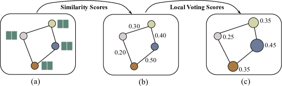
Figure 1: An illustration of the proposed local voting. This graph contains four nodes, each of which has 2 features. Given the input graph, we first compute similarity scores between every pair of connected nodes. In graph (b), we label each edge by the similarity score of its two end nodes. Then we compute the local voting score of each node by averaging the similarity scores with its neighboring nodes. In graph (c), we label each node by its local voting score and a bigger node indicates a higher score.

In this work, we propose the topology-aware pooling (TAP) layer that encodes topology information in ranking scores for node selection. We also propose a graph connectivity term in the computation of ranking scores, which encourages better graph connectivity in the coarsened graph. Based on our TAP layer, we propose the topology-aware pooling networks for graph representation learning.

3.1 Topology-Aware Pooling Layer

3.1.1 Graph Pooling via Node Sampling

Pooling operations are important for deep models on image and NLP tasks that they help enlarge receptive fields and reduce computational cost. They are locality-based operations that extract high-level features from local regions. When generalizing GNNs and GCNs to graph structured data, graph pooling is an important yet challenging topic. Recently, two families of graph pooling methods are proposed. One treats the graph pooling as a node clustering problem while the other one treats graph pooling as a node sampling problem. Both of them are developed to scale down the size of node representations and learn new representations. Formally, given a graph $G=(A,H)$ with the adjacency matrix $A\in\{0,1\}^{n\times n}$ and the feature matrix $H\in\mathbb{R}^{n\times d}$, graph pooling produces a new graph $G^{\prime}$ with $k$ nodes. The new graph $G^{\prime}$ can be represented by its adjacency matrix $A^{\prime}\in\{0,1\}^{k\times k}$ and feature matrix $H^{\prime}\in\mathbb{R}^{k\times d}$. In this work, we follow [12, 11] and treat the graph pooling as a node sampling problem, which learns the importance of different nodes in the original graph $G$ and samples the top $k$ important nodes to form the new graph $G^{\prime}$. Existing methods [12, 11] generate node importance scores based on a globally-shared projection vector that projects feature vectors to scalars. Each scalar is an importance score indicating the importance of the corresponding node. However, these methods do not explicitly consider graph topology information when performing graph pooling, thereby leading to constrained network capability.

In this section, we propose the topology-aware pooling (TAP) layer that performs nodes sampling by considering the graph topology. Specifically, the node ranking score is obtained from two voting processes: local voting and global voting. For any node, the local voting computes its importance based on the similarities with its neighboring nodes, while the global voting evaluates its global importance in the entire graph. Altogether, these two procedures are jointly learned to sort all nodes in the original graph, and then the top $k$ nodes are selected to form the new graph.

3.1.2 Local Voting

Max pooling operations on grid-like data are performed in local regions. Inspired by this, we propose the local voting to measure node importance within a local region, which explicitly incorporates graph topology and local information. Specifically, we compute the similarity scores between each node and its neighboring nodes. The score for a node $i$ is the mean value of the similarity scores with its neighboring nodes. The resulting score for a node indicates the similarity between this node and its neighboring nodes. If a node has a high local voting score, it can highly represent a local graph that consists of it and its neighboring nodes. Formally, given a graph $G=(A,H)$ with the adjacency matrix $A\in\mathbb{R}^{n\times n}$ and the feature matrix $H\in\mathbb{R}^{n\times d}$, the local voting is expressed as

$$R=HH^{T}\in\mathbb{R}^{n\times n},$$ (1)

$$\hat{R}=R\circ(\hat{D}^{-1}\hat{A})\in\mathbb{R}^{n\times n},$$

$$\mathbf{y}^{L}=\mbox{softmax}(\frac{1}{n}\hat{R}\mathbf{1}_{n})\in\mathbb{R}^{n},$$

where $\hat{A}=A+I$ is used to add self-loops, $\hat{D}$ is the diagonal degree matrix with $\hat{D}_{ii}=\sum_{j}\hat{A}_{ij}$, $\circ$ denotes the element-wise matrix multiplication operation, $\mathbf{1}_{n}\in\mathbb{R}^{n}$ denotes a $n$-dimensional vector with all ones, and $\mbox{softmax}(\cdot)$ denotes an element-aware softmax operation.

Suppose $H$ is a matrix with node features, denoted as $H$=$\{\mathbf{h}_{1},\mathbf{h}_{2},\cdot\cdot\cdot,\mathbf{h}_{n}\}^{T}$. For node $i$, its feature is represented as $\mathbf{h}_{i}\in\mathbb{R}^{d}$. We first compute the similarity matrix $R$ based on node features. Specifically, for any node $i$ and node $j$, their similarity score $r_{ij}$ is obtained by the dot product between $\mathbf{h}_{i}$ and $\mathbf{h}_{j}$. Since $R$ contains similarity scores for all node pairs in the graph, we perform an element-wise matrix multiplication between the similarity matrix $R$ and the normalized adjacency matrix $\hat{D}^{-1}\hat{A}$, resulting a matrix $\hat{R}$ where similarity scores for non-connected nodes are all zeros. To this end, each row vector $\hat{\mathbf{r}}_{i}$ in $\hat{R}$ represents similarity scores between the node $i$ and its neighborhood. Next, for the node $i$, we average its all similarity scores to indicate its importance within its local neighbors. Finally, we apply softmax function to obtain the final score vector, denoted as $\mathbf{y}^{L}=[y^{L}_{1},y^{L}_{2},\cdot\cdot\cdot,y^{L}_{n}]^{T}$ and $\sum_{i}y^{L}_{i}=1$.

Our proposed local voting essentially encodes local information from neighborhood and explicitly incorporates graph topology information. The node with a higher score indicates it has higher similarities with its neighbors and hence tends to be more important. Typically, by scoring each node based on local information, local voting achieves a similar objective as the max pooling operation on images. Max pooling on grid-like data keeps the most salient features within a local region. Similarly, our local voting regulates local information and encourages to select the most important nodes within a local region when forming the new graph. Notably, our proposed local voting considers both graph topology information and node features. Node features are used to compute the closeness between different nodes. In addition, we have several ways to compute closeness between two vectors, such as inner product, concatenation, and Gaussian function. In this work, we choose to employ the inner product since it has been proven as a simple yet effective solution [13]. In practice, we can employ learnable weights to make the model more powerful. Specifically, we can add a learnable weight matrix $W_{r}$ to the computation of interaction matrix $R$ that $R=HW_{r}H^{T}$. Figure 1 provides an illustration of our proposed local voting operation.

3.1.3 Global Voting

For each node, local voting essentially shows its “local” role within a local region. However, different from grid-like data such as images, local neighborhood regions within graphs are “overlapped”. We can not rely on local salient features only to perform graph pooling. In this section, we introduce our proposed global voting to evaluate “global” role for each node. Intuitively, local voting shows the importance of a node within its neighborhood, while global voting shows how important its neighbor region (including itself) is in the entire graph. Typically, the neighbor region of a node can be treated as a sub-graph and the center of this sub-graph is the node itself. Such a sub-graph may also carry important information. For example, in a graph representing a protein, atoms are nodes and bonds are edges. Then a sub-graph contains an atom and its neighboring atoms. Certain sub-graphs can represent vital units and indicate the functionality of the entire protein. Hence, such information should be captured in graph pooling. We propose global voting to measure the importance of different subgraphs in the entire graph. Formally, the global voting is express as

$$\hat{H}=\hat{D}^{-1}\hat{A}H\in\mathbb{R}^{n\times n}, \mathbf{y}^{G}=\mbox{softmax}(\hat{H}\mathbf{p})\in\mathbb{R}^{n},$$ (2)

where $\mathbf{p}\in\mathbb{R}^{d}$ is a trainable projection vector, and $\mbox{softmax}(\cdot)$ denotes an element-aware softmax operation. We first aggregate neighbor information for each node, through which the new features of a node represent the information of its sub-graph. After that, we perform the scalar projection $\mathbf{p}$ on the structure-aggregated feature matrix $\hat{H}$ and obtain the score vector $\mathbf{y}^{G}$. The projection vector $\mathbf{p}$ is learnable and shared by all nodes in the graph. In this way, the element $y^{G}_{i}$ in $\mathbf{y}^{G}$ indicates the importance of node $i$ and its sub-graph based on the globally shared vector.

Note that the computation of global voting is similar to the recently proposed SortPool [12] and top-k pooling [11]. However, we explicitly consider the topology information to generate $\hat{H}$ while SortPool and top-k pooling may ignore such information. Without topology information, the capacity of networks is restricted and the functionalities of sub-graphs may be neglected. Our proposed global voting measures the node importance in a global manner and considers both node features and graph topology information.

3.1.4 Graph Pooling Layer

The local voting measures the local similarities between each node and its neighborhood, and the global voting captures the importance of different neighbor regions in the entire graph. Altogether, we combine these two to measure the importance of different nodes so that topology information is explicitly considered. Specifically, the final sorting vector $\mathbf{y}$ is computed as the summation of $\mathbf{y}^{L}$ and $\mathbf{y}^{G}$. Then based on the sorting vector $\mathbf{y}$, we rearrange the order of all the nodes in the original graph and sample the top $k$ important nodes to form a new graph. Formally, our proposed TAP layer can be expressed as

$$\mathbf{y}=\mathbf{y}^{L}+\mathbf{y}^{G}\in\mathbb{R}^{n}, \mbox{idx}=\mbox{rank}(\mathbf{y},k)\in\mathbb{R}^{k},$$ (3)

$$H^{\prime}=H_{\mbox{idx},\ :}\ \in\mathbb{R}^{k\times d}, A^{\prime}=A_{\mbox{idx},\ \mbox{idx}}\ \in\mathbb{R}^{k\times k},$$

where $k$ is a pre-defined number indicating the number of nodes in the output graph, $\mbox{rank}(\mathbf{y},k)$ is the operation for node sampling, which returns the indexes of top-k values in $\mathbf{y}$. The idx is a list of indexes indicating the selected nodes. $H_{\mbox{idx},\ :}$ is a row-aware extractor on feature matrix to obtain the feature matrix $H^{\prime}$ for the new graph. $A_{\mbox{idx},\ \mbox{idx}}$ produces the new adjacency matrix based on the node connections in the original graph. With the ranking procedure, only the top-k important nodes are selected according to the values in $\mathbf{y}$. Then the new feature matrix $H^{\prime}$ and adjacency matrix $A^{\prime}$ are obtained following the extraction process. Notably, our TAP layer introduces negligibly additional parameters, since the only used parameters include the linear transformation matrix $W_{r}$ and the projection vector $\mathbf{p}$.

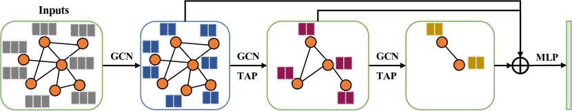
Figure 2: An illustration of the topology-aware pooling network. $\oplus$ denotes the concatenation operation of feature vectors. Each node in the input graph contains three features. We use a GCN layer to transform the feature vectors into low-dimensional representations. We stack two blocks, each of which consists of a GCN layer and a TAP layer. A global reduction operation such as max-pooling is applied to the outputs of the first GCN layer and TAP layers. The resulting feature vectors are concatenated and fed into the final multi-layer perceptron for prediction.

3.2 Graph Connectivity Term

Our proposed TAP layer computes the ranking scores by using similarity scores between nodes in the graph, thereby regarding topology information in the graph. However, the coarsened graph generated by the TAP layer may suffer from the problem of isolated nodes. In sparsely connected graphs, some nodes have a very small number of neighboring nodes or even only themselves. Suppose node $i$ only connects to itself. The local voting score of node $i$ is the similarity score to itself, which may result in high local voting scores, thereby generating high ranking scores in the graph. The resulting graph can be very sparsely connected, which completely loses the original graph structure. In the extreme situation, the coarsened graph can contain only isolated nodes without any connectivity. This can inevitably hurt the model performance.

To overcome the limitation of TAP layer and encourage better connectivity in the selected graph, we propose to add a graph connectivity term to the computation of ranking scores. To this end, we use node degrees as an indicator for graph connectivity and add degree values to their ranking scores such that densely-connected nodes are preferred during nodes selection. By using the node degree as the graph connectivity term, the ranking score of node $i$ is computed as

$$s_{i}=y_{i}+\lambda\frac{d_{i}}{n},$$ (4)

where $y_{i}$ is the ranking score achieved in Eq. (3) of node $i$, $d_{i}$ is the degree of node $i$, and $\lambda$ is a hyper-parameter that sets the importance of the graph connectivity term to the computation of ranking scores. The graph connectivity term can overcome the limitation of the TAP layer. The computation of ranking scores now considers nodes degrees and gives rise to better connectivity in the resulting graph. A better connected coarsened graph is expected to retain more graph structure information, thereby leading to better model performance.

3.3 Topology-Aware Pooling Networks

Based on our proposed TAP layer, we build a family of networks known as topology-aware pooling networks (TAPNets) for graph classification tasks. In TAPNets, we firstly apply a graph embedding layer to produce low-dimensional representations of nodes in the graph, which helps to deal with some datasets with very high-dimensional input feature vectors. Here, we use a GCN layer [14] for node embedding. After the embedding layer, we stack several blocks, each of which consists of a GCN layer for high-level feature extraction and a TAP layer for graph coarsening. In the $i^{th}$ TAP layer, we use a hyper-parameter $k^{(i)}$ to control the number of nodes in the sampled graph. We feed the output feature matrices of the graph embedding layer and TAP layers to a classifier.

In TAPNets, we use a multi-layer perceptron as the classifier. We first transform network outputs to a one-dimensional vector. Global max and average pooling operations are two popular ways for the transformation, which reduce the spatial size of feature matrices to 1. Recently, [15] proposed to use the summation function that results in promising performances. In TAPNets, we concatenate transformation output vectors produced by the global pooling operations using max, averaging, and summation, respectively. The resulting feature vector is fed into the classifier. Figure 2 illustrates a sample TAPNet with two blocks.

3.4 Auxiliary Link Prediction Objective

Multi-task learning has shown to be effective across various machine learning tasks [16, 7]. It can leverage useful information in multiple related tasks, thereby leading to better generalization and performance. In this section, we propose to add an auxiliary link prediction objective during training by using a by-product of our TAP layer. In Eq. (1), we compute the similarity scores $R$ between every pair of nodes in the graph. By applying an element-wise $\mbox{softmax}(\cdot)$ on $R$, we can obtain a link probability matrix $\tilde{R}\in\mathbb{R}^{n\times n}$ with each element $\tilde{r}_{ij}$ measures the likelihood of a link between node $i$ and node $j$ in the graph. With the adjacency matrix $A$, we compute the auxiliary link prediction loss as

$$loss_{aux}=\frac{1}{n^{2}}\sum_{i=1}^{n}\sum_{j=1}^{n}f\left(\tilde{R}_{ij},A_{ij}\right),$$ (5)

where $f(\cdot,\cdot)$ is a loss function that computes the distance between the link probability matrix $\tilde{R}$ and the adjacency matrix $A$.

Note that the adjacency matrix used as the link prediction objective is directly derived from the original graph. Since the TAP layer extracts a sub-graph from the original one, the connectivity between two nodes in the sampled graph is the same as that in the original graph. This means the adjacency matrices in deeper networks are still using the original graph structure. Compared to auxiliary link prediction in DiffPool [7] that uses the learned adjacency matrix as objective, our method uses the original links, thereby providing more accurate information. This can also be clearly observed in the experimental studies in Sections 4.2 and 4.3.

TABLE I: Comparisons between TAPNets and other models in terms of graph classification accuracy (%) on social network datasets including COLLAB, IMDB-BINARY, IMDB-MULTI, REDDIT-BINARY, REDDIT-MULTI5K and REDDIT-MULTI12K datasets.

	COLLAB	IMDB-B	IMDB-M	RDT-B	RDT-M5K	RDT-M12K
# graphs	5000	1000	1500	2000	4999	11929
# nodes	74.5	19.8	13.0	429.6	508.5	391.4
# classes	3	2	3	2	5	11
WL [17]	78.9 $\pm$ 1.9	73.8 $\pm$ 3.9	50.9 $\pm$ 3.8	81.0 $\pm$ 3.1	52.5 $\pm$ 2.1	44.4 $\pm$ 2.1
PSCN [18]	72.6 $\pm$ 2.2	71.0 $\pm$ 2.2	45.2 $\pm$ 2.8	86.3 $\pm$ 1.6	49.1 $\pm$ 0.7	41.3 $\pm$ 0.8
DGCNN [12]	73.8	70.0	47.8	-	-	41.8
DIFFPOOL [7]	75.5	-	-	-	-	47.1
g-U-Net [11]	77.5 $\pm$ 2.1	75.4 $\pm$ 3.0	51.8 $\pm$ 3.7	85.5 $\pm$ 1.3	48.2 $\pm$ 0.8	44.5 $\pm$ 0.6
GIN [15]	80.6 $\pm$ 1.9	75.1 $\pm$ 5.1	52.3 $\pm$ 2.8	92.4 $\pm$ 2.5	57.5 $\pm$ 1.5	-
TAPNet (ours)	84.9 $\pm$ 1.8	79.9 $\pm$ 4.5	56.2 $\pm$ 3.1	94.6 $\pm$ 1.8	57.3 $\pm$ 1.5	49.4 $\pm$ 1.7

4 Experimental Studies

In this section, we evaluate our methods and networks on graph classification tasks using bioinformatics and social network datasets. We conduct ablation experiments to evaluate the contributions of the TAP layer and each term in it to the overall network performance.

4.1 Experimental Setup

We evaluate our methods using social network datasets and bioinformatics datasets. They share the same experimental setups except for minor differences. The node features in social network networks are created using one-hot encodings of node degrees. The nodes in bioinformatics have categorical features. We use the TAPNet proposed in Section 3.3 that consists of one GCN layer and three blocks. The first GCN layer is used to learn low-dimensional representations of nodes in the graph. Each block is composed of one GCN layer and one TAP layer. All GCN and TAP layers output 48 feature maps. We use Leaky ReLU [19] with a slop of 0.01 to activate the outputs of GCN layers. The three TAP layers in the networks select numbers of nodes that are proportional to the nodes in the graph. We use the rates of 0.8, 0.6, and 0.4 in three TAP layers, respectively. We use $\lambda=0.1$ to control the importance of the graph connectivity term in the computation of ranking scores. Dropout [20] is applied to the input feature matrices of GCN and TAP layers with keep rate of 0.7. We use a two-layer feed-forward network as the network classifier. Dropout with keep rate of 0.8 is applied to input features of two layers. We use ReLU activation function on the output of the first layer on DD, PTC, MUTAG, COLLAB, REDDIT-MULTI5K, and REDDIT-MULTI12K datasets. We use ELU [21] for other datasets. We train our networks using Adam optimizer [22] with a learning rate of 0.001. To avoid over-fitting, we use $L_{2}$ regularization with $\lambda=0.0008$. All models are trained using one NVIDIA GeForce RTX 2080 Ti GPU.

We compare our method with several state-of-the-art baselines. Weisfeiler-Lehman subtree kernel (WL) [17] is treated as the most effective kernel method for graph representation learning. PSCN [18] learns node representations from neighborhood and uses a canonical node ordering for graph representations. DGCNN [12] applies several GCN layers and proposes SortPool to perform graph pooling by sorting and selecting nodes. DiffPool [7] is developed based on GraphSage [23] and proposes a hierarchical pooling technique, which learns to perform node clustering to build the new graph. g-U-Net [11] proposes top-$k$ pooling that employs a projection vector to compute the rank score for each node. The graph topology is not considered when computing rank scores. SAGPool [24] is similar to top-$k$ pooling and encodes topology information. The graph connectivity issue is not tackled in SAGPool. GIN [15] is the graph isomorphism network, whose representational power is shown to be similar to the power of the WL test. EigenPool [25] is another node-clustering method that is based on graph Fourier transform and utilizes local structures when performing node clustering. HaarPool [26] employs Haar basis and the compressive Haar transforms to generate a sparse characterization of the input graph while preserving structure information.

TABLE II: Comparisons between TAPNets and other models in terms of graph classification accuracy (%) on bioinformatics datasets including DD, PTC, MUTAG, and PROTEINS datasets.

	DD	PTC	MUTAG	PROTEINS
# graphs	1178	344	188	1113
# nodes	284.3	25.5	17.9	39.1
# classes	2	2	2	2
WL [17]	78.3 $\pm$ 0.6	59.9 $\pm$ 4.3	90.4 $\pm$ 5.7	75.0 $\pm$ 3.1
PSCN [18]	76.3 $\pm$ 2.6	60.0 $\pm$ 4.8	92.6 $\pm$ 4.2	75.9 $\pm$ 2.8
DGCNN [12]	79.4 $\pm$ 0.9	58.6 $\pm$ 2.4	85.8 $\pm$ 1.7	75.5 $\pm$ 0.9
SAGPool [24]	76.5	-	-	71.9
DIFFPOOL [7]	80.6	-	-	76.3
g-U-Net [11]	82.4 $\pm$ 2.9	64.7 $\pm$ 6.8	87.2 $\pm$ 7.8	77.6 $\pm$ 2.6
GIN [15]	82.0 $\pm$ 2.7	64.6 $\pm$ 7.0	90.0 $\pm$ 8.8	76.2 $\pm$ 2.8
EigenPool [25]	0.786	-	0.801	0.766
HaarPool [26]	-	-	90.0 $\pm$ 3.6	80.4 $\pm$ 1.8
TAPNet (ours)	84.6 $\pm$ 3.5	73.4 $\pm$ 5.8	93.8 $\pm$ 6.0	80.8 $\pm$ 4.5

4.2 Graph Classification Results on Social Network Datasets

We conduct experiments on graph classification tasks to evaluate our proposed methods and TAPNets. We use 6 social network datasets; those are COLLAB, IMDB-BINARY, IMDB-MULTI, REDDIT-BINARY, REDDIT-MULTI5K and REDDIT-MULTI12K [27] datasets. Note that REDDIT datasets are popular large datasets used for network embedding learning in terms of graph size and number of graphs [7, 15]. Since there is no feature for nodes in social networks, we create node features by following the practices in [15]. In particular, we use one-hot encodings of node degrees as feature vectors for nodes in social network datasets. On these datasets, we perform 10-fold cross-validation as in [12] with 9 folds for training and 1 fold for testing. To ensure fair comparisons, we do not use the auxiliary link prediction objective in these experiments. We compare our TAPNets with other state-of-the-art models in terms of graph classification accuracy. The comparison results are summarized in Table I. We can observe from the results that our TAPNets significantly outperform previous best models on most social network datasets by margins of 4.3%, 4.8%, 3.9%, 2.2%, and 2.3% on COLLAB, IMDB-BINARY, IMDB-MULTI, REDDIT-BINARY, and REDDIT-MULTI12K datasets, respectively. The promising performances, especially on large datasets such as REDDIT, demonstrate the effectiveness of our methods. Note that the superior performances over g-U-Net [11] show that our TAP layer can produce better-coarsened graph than that using the top-$k$ pooling layer.

4.3 Graph Classification Results on Bioinformatics Datasets

To fully evaluate our methods, we conduct experiments on graph classification tasks using 4 bioinformatics datasets; those are DD  [28] , PTC  [29] , MUTAG  [30] , and PROTEINS  [31]  [15] datasets. Notably, nodes in bioinformatics datasets have categorical features. In these experiments, we do not use the auxiliary link prediction objective. We compare our TAPNets with other state-of-the-art models in terms of graph classification accuracy without using the auxiliary link prediction term in loss function. The comparison results are summarized in Table II. We can observe from the results that our TAPNets achieve significantly better results than other models by margins of 2.2%, 8.7%, 3.8%, and 0.4% on DD, PTC, MUTAG, and PROTEINS datasets, respectively. Notably, some bioinformatics datasets such as PTC and MUTAG are much smaller than social network datasets in terms of number of graphs and number of nodes in graphs. The promising results on these small datasets demonstrate that our methods can achieve good generalization and performances without the risk of over-fitting. Also, the superior performances over SAGPool on DD and PROTEINS datasets demonstrate that our methods can better capture the topology information.

4.4 Comparison with Other Graph Pooling Layers

TABLE III: Comparisons between different pooling operations based on the same TAPNet architecture in terms of the graph classification accuracy (%) on PTC, IMDB-MULTI, and REDDIT-BINARY datasets.

Model	PTC	IMDB-M	RDT-B
Net${}_{\mbox{diff}}$	70.9	54.9	92.1
Net${}_{\mbox{sort}}$	70.6	54.8	92.3
Net${}_{\mbox{top-}k}$	71.5	55.2	92.8
TAPNet	73.4	56.2	94.6

It may be argued that our TAPNets achieve promising results by employing superior networks. In this section, we conduct experiments on the same TAPNet architecture to compare our TAP layer with other graph pooling layers; those are DIFFPOOL, SortPool, and top-$k$ pooling layers. We denote the networks with the TAPNet architecture while using these pooling layers as Net${}_{\mbox{diff}}$, Net${}_{\mbox{sort}}$, and Net${}_{\mbox{top-}k}$, respectively. We evaluate them on PTC, IMDB-MULTI, and REDDIT-BINARY datasets and summarize the results in Table III. Note that these models use the same experimental setups to ensure fair comparisons. The results demonstrate the superior performance of our proposed TAP layer compared with other pooling layers using the same network architecture.

4.5 Ablation Studies

TABLE IV: Comparisons among TAPNets with and without TAP layers, TAPNet without local voting term (LV), TAPNet without global voting term (GV), TAPNet without graph connection term (GCT), and TAPNet with auxiliary link prediction objective (AUX) in terms of the graph classification accuracy (%) on PTC, IMDB-MULTI, and REDDIT-BINARY datasets.

Model	PTC	IMDB-M	RDT-B
TAPNet w/o TAP	70.6	52.1	91.0
TAPNet w/o LV	72.1	55.3	93.2
TAPNet w/o GV	72.7	55.6	94.1
TAPNet w/o GCT	73.1	55.8	94.2
TAPNet	73.4	56.2	94.6
TAPNet w AUX	73.7	56.4	94.8

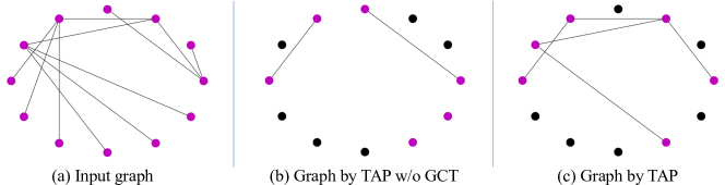
Figure 3: Visualization of coarsened graphs by TAP and TAP w/o GCT. Here, GCT denotes the graph connection term. Based on the input graph (a), the pooling layers select 6 nodes to form new graphs. The nodes that are not selected are colored black. The new graph in (b) generated by TAP w/o GCT is sparsely connected. The one generated by TAP in (c) is shown to be better connected.

In this section, we investigate the contributions of TAP layer and its components in ranking score computation; those are the local voting term (LV), the global voting term (GV)and the graph connectivity term (GCT). We remove TAP layers from TAPNet which we denote as TAPNet w/o TAP. To explore the contributions of terms in ranking scores computation, we separately remove LVs, GVs and GCTs from all TAP layers in TAPNets. We denote the resulting models as TAPNet w/o LV, TAPNet w/o GV and TAPNet w/o GCT, respectively. In addition, we add the auxiliary link prediction objective as described in Section 3.4 in training. We denote the TAPNet using auxiliary training objective as TAPNet w AUX. We evaluate these models on three datasets; those are PTC, IMDB-MULTI, and REDDIT-BINARY datasets.

The comparison results on these datasets are summarized in Table IV. The results show that TAPNets outperform TAPNets w/o TAP by margins of 2.8%, 4.1%, and 3.5% on PTC, IMDB-MULTI, and REDDIT-BINARY datasets, respectively. The better results of TAPNet over TAPNet w/o SST and TAPNet w/o GCT show the contributions of LVs, GVs, and GCTs to performances. It can be observed that TAPNet w AUX achieves better performances than TAPNet, which shows the effectiveness of the auxiliary link prediction objective. To fully study the impact of GCT on TAP layer, we visualize the coarsened graphs generated by TAP and TAP without GCT (denoted as TAP w/o GCT). We select a graph from PTC dataset and illustrate outcome graphs in Figure 3. We can observe from the figure that TAP produces a better-connected graph than that by TAP w/o GCT.

4.6 Parameter Study of TAP

TABLE V: Comparisons among TAPNets with and without TAP layers, and TAPNet without local voting and global voting (LV&GV) in terms of the graph classification accuracy (%), and the number of parameters on REDDIT-BINARY dataset.

Model	Accuracy	#Params	Ratio
TAPNet w/o TAP	91.0	323,666	0.00%
TAPNet w/o LV&GV	91.5	323,666	0.00%
TAPNet	94.6	331,090	2.29%

Since TAP layer employs linear transformation to compute ranking scores, it involves extra trainable parameters to the overall network. Here, we conduct experiments to study the number of parameters in TAPNet. We remove the extra trainable parameters from TAP layers in two ways; those are removing TAP layers from the TAPNet and removing similarity score terms LV and GV from TAP layers. We denote the resulting two networks as TAPNet w/o TAP and TAPNet w/o LV&GV, respectively. The comparison results on REDDIT-BINARY dataset is summarized in Table V. We can see from the results that TAP layers only need 2.29% additional trainable parameters. We believe the negligible usage of extra parameters will not increase the risk of over-fitting but can bring 3.6% and 3.1% performance improvement over TAPNet w/o TAP and TAPNet w/o LV&GV on REDDIT-BINARY dataset. Also, the promising performances of TAPNets on small datasets like PTC and MUTAG in Table II show that TAP layers will not significantly increase the number of trainable parameters or cause the over-fitting problem.

4.7 Performance Study of $\lambda$

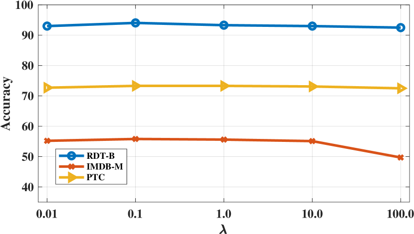
Figure 4: Comparison results of TAPNets using different $\lambda$ values in TAP layers. We report graph classification accuracies on PTC, IMDB-BINARY, and REDDIT-BINARY datasets.

In Section 3.2, we propose to add the graph connectivity term into the computation of ranking scores to improve the graph connectivity in the coarsened graph. It can be seen that $\lambda$ is an influential hyper-parameter in the TAP layer. In this part, we study the impacts of different $\lambda$ values on network performances. We select different $\lambda$ values from the range of 0.01, 0.1, 1.0, 10.0, and 100.0 to cover a reasonable range of values. We evaluate TAPNets using different $\lambda$ values on PTC, IMDB-MULTI, and REDDIT-BINARY datasets.

The results are shown in Figure 4. We can observe that the best performances on three datasets are achieved with $\lambda=0.1$. When $\lambda$ becomes larger, the performances of TAPNet models decrease. This indicates that the graph connectivity term is a plus term for generating reasonable ranking scores but it should not overwhelm the similarity score term that encodes the topology information in ranking scores.

5 Conclusions

In this work, we propose a novel topology-aware pooling (TAP) layer that explicitly encodes the topology information in ranking scores. A TAP layer performs a two-stage voting process that includes the local voting and global voting. The local voting attends each node to its neighboring nodes and uses the average similarity score with its neighboring nodes as its local importance score. The global voting employs a projection vector to compute a similarity score for each node as its global importance score. Then the final ranking score for a node is the combination of its local and global voting scores. The node sampling based on these ranking scores explicitly incorporates the topology information, thereby leading to a better-coarsened graph. Moreover, we propose to add a graph connectivity term to the computation of ranking scores to overcome the isolated problem which a TAP layer may suffer from. Based on the TAP layer, we develop topology-aware pooling networks (TAPNets) for network representation learning. We add an auxiliary link prediction objective to train our networks by employing the similarity score matrix generated in TAP layers. Experimental results on graph classification tasks using both bioinformatics and social network datasets demonstrate that our TAPNets achieve performance improvements as compared to previous models. Ablation Studies show the contributions of our TAP layers to network performance.

References

- [1] K. Simonyan and A. Zisserman, “Very deep convolutional networks for large-scale image recognition,” arXiv preprint arXiv:1409.1556, 2014.
- [2] K. He, X. Zhang, S. Ren, and J. Sun, “Deep residual learning for image recognition,” in Proceedings of the IEEE conference on computer vision and pattern recognition, 2016, pp. 770–778.
- [3] G. Huang, Z. Liu, L. Van Der Maaten, and K. Q. Weinberger, “Densely connected convolutional networks,” in Proceedings of the IEEE conference on computer vision and pattern recognition, 2017, pp. 4700–4708.
- [4] X. Zhang, J. Zhao, and Y. LeCun, “Character-level convolutional networks for text classification,” in Advances in neural information processing systems, 2015, pp. 649–657.
- [5] L. Mou, G. Li, L. Zhang, T. Wang, and Z. Jin, “Convolutional neural networks over tree structures for programming language processing,” in Thirtieth AAAI Conference on Artificial Intelligence, 2016.
- [6] L.-C. Chen, G. Papandreou, I. Kokkinos, K. Murphy, and A. L. Yuille, “Deeplab: Semantic image segmentation with deep convolutional nets, atrous convolution, and fully connected crfs,” IEEE transactions on pattern analysis and machine intelligence, vol. 40, no. 4, pp. 834–848, 2017.
- [7] R. Ying, J. You, C. Morris, X. Ren, W. L. Hamilton, and J. Leskovec, “Hierarchical graph representation learning with differentiable pooling,” in Advances in Neural Information Processing Systems, 2018, pp. 4800–4810.
- [8] H. Gao, Z. Wang, and S. Ji, “Large-scale learnable graph convolutional networks,” in Proceedings of the 24th ACM SIGKDD International Conference on Knowledge Discovery & Data Mining. ACM, 2018, pp. 1416–1424.
- [9] Z. Wang and S. Ji, “Second-order pooling for graph neural networks,” IEEE Transactions on Pattern Analysis and Machine Intelligence, 2020.
- [10] H. Yuan and S. Ji, “Structpool: Structured graph pooling via conditional random fields,” in International Conference on Learning Representations, 2019.
- [11] H. Gao and S. Ji, “Graph U-nets,” in Proceedings of The 36th International Conference on Machine Learning, 2019, pp. 2083–2092.
- [12] M. Zhang, Z. Cui, M. Neumann, and Y. Chen, “An end-to-end deep learning architecture for graph classification,” in Thirty-Second AAAI Conference on Artificial Intelligence, 2018.
- [13] X. Wang, R. Girshick, A. Gupta, and K. He, “Non-local neural networks,” in Proceedings of the IEEE Conference on Computer Vision and Pattern Recognition, 2018, pp. 7794–7803.
- [14] T. N. Kipf and M. Welling, “Semi-supervised classification with graph convolutional networks,” in International Conference on Learning Representations, 2017.
- [15] K. Xu, W. Hu, J. Leskovec, and S. Jegelka, “How powerful are graph neural networks?” in International Conference on Learning Representations, 2019.
- [16] S. Ruder, “An overview of multi-task learning in deep neural networks,” arXiv preprint arXiv:1706.05098, 2017.
- [17] N. Shervashidze, P. Schweitzer, E. J. v. Leeuwen, K. Mehlhorn, and K. M. Borgwardt, “Weisfeiler-lehman graph kernels,” Journal of Machine Learning Research, vol. 12, no. Sep, pp. 2539–2561, 2011.
- [18] M. Niepert, M. Ahmed, and K. Kutzkov, “Learning convolutional neural networks for graphs,” in International conference on machine learning, 2016, pp. 2014–2023.
- [19] B. Xu, N. Wang, T. Chen, and M. Li, “Empirical evaluation of rectified activations in convolutional network,” arXiv preprint arXiv:1505.00853, 2015.
- [20] N. Srivastava, G. Hinton, A. Krizhevsky, I. Sutskever, and R. Salakhutdinov, “Dropout: a simple way to prevent neural networks from overfitting,” The Journal of Machine Learning Research, vol. 15, no. 1, pp. 1929–1958, 2014.
- [21] D.-A. Clevert, T. Unterthiner, and S. Hochreiter, “Fast and accurate deep network learning by exponential linear units (elus),” arXiv preprint arXiv:1511.07289, 2015.
- [22] D. Kingma and J. Ba, “Adam: A method for stochastic optimization,” The International Conference on Learning Representations, 2015.
- [23] W. Hamilton, Z. Ying, and J. Leskovec, “Inductive representation learning on large graphs,” in Advances in Neural Information Processing Systems, 2017, pp. 1024–1034.
- [24] J. Lee, I. Lee, and J. Kang, “Self-attention graph pooling,” in Proceedings of The 36th International Conference on Machine Learning, 2019.
- [25] Y. Ma, S. Wang, C. C. Aggarwal, and J. Tang, “Graph convolutional networks with eigenpooling,” in Proceedings of the 25th ACM SIGKDD International Conference on Knowledge Discovery & Data Mining, 2019, pp. 723–731.
- [26] Y. G. Wang, M. Li, Z. Ma, G. Montufar, X. Zhuang, and Y. Fan, “Haar graph pooling,” in International conference on machine learning, 2020.
- [27] P. Yanardag and S. Vishwanathan, “A structural smoothing framework for robust graph comparison,” in Advances in Neural Information Processing Systems, 2015, pp. 2134–2142.
- [28] P. D. Dobson and A. J. Doig, “Distinguishing enzyme structures from non-enzymes without alignments,” Journal of molecular biology, vol. 330, no. 4, pp. 771–783, 2003.
- [29] H. Toivonen, A. Srinivasan, R. D. King, S. Kramer, and C. Helma, “Statistical evaluation of the predictive toxicology challenge 2000–2001,” Bioinformatics, vol. 19, no. 10, pp. 1183–1193, 2003.
- [30] N. Wale, I. A. Watson, and G. Karypis, “Comparison of descriptor spaces for chemical compound retrieval and classification,” Knowledge and Information Systems, vol. 14, no. 3, pp. 347–375, 2008.
- [31] K. M. Borgwardt, C. S. Ong, S. Schönauer, S. Vishwanathan, A. J. Smola, and H.-P. Kriegel, “Protein function prediction via graph kernels,” Bioinformatics, vol. 21, no. suppl_1, pp. i47–i56, 2005.