Abstract

Given $k$ pre-trained classifiers and a stream of unlabeled data examples, how can we actively decide when to query a label so that we can distinguish the best model from the rest while making a small number of queries? Answering this question has a profound impact on a range of practical scenarios. In this work, we design an online selective sampling approach that actively selects informative examples to label and outputs the best model with high probability at any round. Our algorithm can be used for online prediction tasks for both adversarial and stochastic streams. We establish several theoretical guarantees for our algorithm and extensively demonstrate its effectiveness in our experimental studies.

1 INTRODUCTION

Model selection from a set of pre-trained models is an emerging problem in machine learning and has implications in several practical scenarios. Industrial examples include cases in which a telecommunication company or a flight booking company has multiple ML models trained over different sliding windows of data and hopes to pick the one that performs the best on a given day. For many real-world problems, unlabeled data is abundant and can be inexpensively collected, while labels are expensive to acquire and require human expertise. Consequently, there is a need to robustly identify the best model under limited labeling resources. Similarly, one often needs reasonable predictions for the unlabeled data while keeping the labeling budget low.

Depending on the data availability, one can consider two settings: (i) the pool-based setting assumes that the learner has access to a pool of unlabeled data, and she can select informative data samples from the pool to achieve her task, and (ii) the online setting assumes the data is arriving one example at a time (i.e., in a stream), and the learner decides to ask for the example’s label on the go or to just throw it away. While offering fewer options on which data to label, this setting alleviates the scalability challenge of storing and processing a large pool of examples in the pool-based setting.

Another important aspect is the nature of the data: the instance-label pairs might be sampled i.i.d. from a fixed distribution, or chosen adversarially by an adversary. While sometimes the i.i.d. assumption is reasonable, there are practical scenarios where this assumption fails to hold. These include cases where there are temporal or spatial dependencies or non-stationarities in the dataset/stream. In these situations, it may be safer not to make assumptions on the data and rather consider worst-case data streams.

Contributions

We develop a novel, principled and efficient model selection approach –Model Picker– for the online setting. Our query strategy is randomized and leverages hypothetical query answers to decide which data examples are likely to be informative for identifying the best model. We prove that our algorithm has no regret for adversarial streams, i.e., its performance for sequential label prediction is close to the best model for that stream in hindsight. Our bounds match (up to a constant) those of existing online algorithms that have access to all labels. We also establish bounds on the number of label queries and the quality of the output model of Model Picker. We furthermore conduct extensive experiments, comparing our algorithm with a range of other methods. To reach the same accuracy, competing methods can often require up to 2.5$\times$ more labels. Apart from the relative performance, on the ImageNet dataset, Model Picker requires a mere 13% labeled instances to select the best among 102 pre-trained models with 90% confidence, while having up to 1.3$\times$ lower regret. These results establish Model Picker as the state-of-the-art for this problem. We also make everything open and reproducible.

2 RELATED WORKS

Our approach relates to several bodies of literature. For each related area, we reference similar works that match the objective of our paper.

Active Model Selection

Madani et al. (2004) develop their method for the online setting. They seek to identify the best model via probing models, one at a time, with i.i.d. samples, while having a fixed budget for the number of probes. In contrast, our approach applies even to adversarial streams and allows one to make predictions online, while minimizing the number of queries made. Most of other previous works (Sawade et al., 2012; Gardner et al., 2015; Ali et al., 2014; Sawade et al., 2010; Katariya et al., 2012; Kumar and Raj, 2018; Leite and Brazdil, 2010) focus on pool-based sampling of informative instances, where the learner ranks the entire pool of unlabeled data and greedily selects the most informative examples. This setting substantially differs from the streaming setting, and we focus on the latter for reasons of scalability and applicability to many real-world situations.

Active Learning

Active learning aims to query the label of those instances that help improving the training of classifiers, rather than selecting among pre-trained models. Here we review those methods that can potentially be adapted for model selection. The celebrated query-by-committee (QBC) paradigm (Seung et al., 1992) forms a committee of classifiers to vote on the labeling of incoming examples. The query decision is made based on the degree of disagreement among the committee members. The general strategy is to query those instances that help the learner prune the committee and only keep those classifiers with higher accuracies. There are other QBC approaches in active learning, such as Cohn et al. (1994); McCallum and Nigam (1998); Abe and Mamitsuka (1998); Melville and Mooney (2004); Settles and Craven (2008); Zhu et al. (2007). One limitation of these algorithms is that they often focus on pool-based sampling, which limits their scalability. Several other approaches consider active learning in the streaming setting. The seminal works of Dasgupta et al. (2008) and Balcan et al. (2009), followed by Beygelzimer et al. (2010); Zhang and Chaudhuri (2014), use disagreement-based strategies. The idea of using importance weights in active learning is studied by a series of works including Beygelzimer et al. (2008); Sugiyama (2006); Beygelzimer et al. (2011); Bach (2007), where importance weights are introduced to correct sampling bias and provide statistically consistent convergence to the optimal classifier in the PAC learning setting. All of the above approaches on stream-based active learning focus on i.i.d. streams and try to improve the supervised training of classifiers, whereas our approach applies to the more general adversarial streams and performs no training.

Online Learning and Bandits

Sequential label prediction is an important problem in online learning. The setting closest to ours is label-efficient prediction (LEP) (Cesa-Bianchi et al., 2005), where they query the label with a fixed probability at each round, and that probability also appears in the regret bound. However, we use the side information of the models predictions to adapt the probability of querying to the information content of the instance at hand, thereby significantly reducing the required labels in practice and lowering the regret, as demonstrated theoretically and in our experiments. Moreover, there is no study of the quality of the model outputted at the end of the stream, for neither adversarial nor stochastic streams. Another problem similar to ours is consistent online learning (Karimi et al., 2019; Altschuler and Talwar, 2018), where the learner seeks to minimize the number of switches of her actions, while observing the loss every round, even if she does not update her strategy. In our setting, however, we do not know the loss in the rounds we do not query. Similar challenges arise in the multi-armed bandit literature. In a way, our setup lies between the usual prediction with experts advice and multi-armed bandit problems. Our algorithm is related in spirit to the EXP3 algorithm (Auer et al., 2002) for adversarial bandits. The key difference is that EXP3 uses the probability of selecting an arm to construct an unbiased loss estimator, whereas we consider the probability of observing the whole loss. While similar in spirit, the standard EXP3 analysis fails to yield a regret bound, as discussed in the footnote of page 3.

3 PROBLEM STATEMENT AND BACKGROUND

Assume that we have $k$ pre-trained classifiers (experts). Let $\mathcal{X}$ and $\mathcal{C}$ be the set of all possible inputs and classes, respectively. Our sequential prediction problem is a game played in rounds. Consider a stream of data $\{(x_{t},c_{t})\in\mathcal{X}\times\mathcal{C}\}_{t\geq 1}$ generated by an unknown mechanism. At round $t$, $x_{t}$ together with all classifiers predictions $\bm{p}_{t}\in\mathcal{C}^{k}$ is revealed to the learner. She then selects one of the experts $I_{t}\in[k]$ and incurs a loss of 1 if that expert misclassifies $x_{t}$. Finally, the learner decides whether to query the label $c_{t}$. If no query is made, then $c_{t}$ remains hidden, otherwise, the learner observes $c_{t}$ and the loss $\bm{\ell}_{t}\in\{0,1\}^{k}$ defined as $\bm{\ell}_{t,i}=\mathbb{I}_{\{\bm{p}_{t,i}\neq c_{t}\}}$, with $\mathbb{I}_{\{\cdot\}}$ being the indicator function. Note that $I_{t}$ can only depend on the past inputs and the observed labels. The goal of the learner is to select $I_{t}$ in such a way that up to any round $T$, the total misclassifications she makes is close to the total mistakes of the best expert up to time $T$ in hindsight. This performance measure is formalized as the regret of the learner:

$$\mathcal{R}_{T}=\textstyle\sum_{t=1}^{T}\bm{\ell}_{t,I_{t}}-\min_{i\in[k]}\sum_{t=1}^{T}\bm{\ell}_{t,i}.$$

A prediction strategy satisfying $\limsup_{t\to\infty}\mathcal{R}_{t}/t\leq 0$, is called a no-regret algorithm.

If the stream is generated by sampling $(x_{t},c_{t})$ i.i.d. from a fixed distribution, it is called a stochastic stream, otherwise we call it adversarial, as if an oblivious adversary has chosen the stream for the learner. It is known (Hazan, 2019) that if the learner follows a deterministic strategy, she can be forced by the adversary to have linear regret. Hence, the learner should randomize and select $I_{t}\sim\bm{w}_{t}$, where $\bm{w}_{t}$ is some distribution over the experts, reflecting how good the learner thinks the experts are at round $t$. In this case, we are interested in the expected regret $\operatorname{\mathbb{E}}[\mathcal{R}_{T}]$, where the expectation is w.r.t. the (possible) randomness in the stream, as well as the randomness of the learner. By the tower property of expectation, $\operatorname{\mathbb{E}}[\bm{\ell}_{t,I_{t}}]=\operatorname{\mathbb{E}}[\operatorname{\mathbb{E}}[\bm{\ell}_{t,I_{t}}\mid\bm{w}_{t},\bm{\ell}_{t}]]=\operatorname{\mathbb{E}}\langle\bm{w}_{t},\bm{\ell}_{t}\rangle$, and hence, we could write

$$\operatorname{\mathbb{E}}[\mathcal{R}_{T}]=\operatorname{\mathbb{E}}\big{[}\textstyle\sum_{t=1}^{T}\langle\bm{w}_{t},\bm{\ell}_{t}\rangle-\min_{i\in[k]}\sum_{t=1}^{T}\bm{\ell}_{t,i}\big{]}.$$

On top of the preceding task, it is often desirable that at each round $t$, the learner recommends (or outputs) an expert $\pi_{t}$ as the best expert so far. This recommendation is suited for model selection tasks, where one needs not only the predictions per round, but also a recommendation about which classifier is the best one. We measure the quality of $\pi_{t}$ in two ways: the probability of returning the true best model of the stream so far (identification probability), and the gap between the accuracy of the recommended model and the best one (accuracy gap). The choice of measure depends on the application: if one is interested only in identifying the best model, then the first measure, and if one just cares about getting a model that has an accuracy close to the best classifier, then the second measure is more relevant.

4 ALGORITHM AND ANALYSIS

In this section we set up the notation and present the Model Picker algorithm, along with several theoretical results regarding its performance.

4.1 The Algorithm

At any round $t$, our algorithm, based on the predictions $\bm{p}_{t}$ and current distribution $\bm{w}_{t}$ decides to query the label with probability $q_{t}$ (to be determined later). Let $Q_{t}\sim\mathrm{Ber}(q_{t})$ be the indicator of querying. Our algorithm then constructs a loss estimate $\hat{\bm{\ell}}_{t}=\bm{\ell}_{t}/q_{t}\cdot Q_{t}$. With this trick, we can think that the learner observes the loss sequence $\{\hat{\bm{\ell}}_{t}\}_{t\geq 1}$. We then construct $\bm{w}_{t}$ similar to the Exponential Weights (EW) algorithm (Littlestone and Warmuth, 1994) for this loss estimate sequence and with decaying learning rates $\{\eta_{t}\}$. The detailed algorithm is depicted in Algorithm 1. In what follows, we also set $\widehat{\bm{L}}_{t}=\sum_{s\leq t}\hat{\bm{\ell}}_{s}$ and $\bm{L}_{t}=\sum_{s\leq t}\bm{\ell}_{s}$.

Set $\widehat{\bm{L}}_{0,i}=0$ for all $i\in[k]$

for $t=1,2,\ldots$ do

      

      $\eta_{t}\coloneqq\sqrt{(\log k)/(2t)}$

      Compute the distribution $\bm{w}_{t}$ over models, with $\bm{w}_{t,i}\propto\exp\{-\eta_{t}\widehat{\bm{L}}_{t-1,i}\}$

      Get predictions $\bm{p}_{t}$ of models for the observed data instance $x_{t}$

      Recommend $\pi_{t}:=\operatorname*{arg\,max}_{i\in[k]}\bm{w}_{t,i}$ as the best model up to round $t$

      Sample $I_{t}\sim\bm{w}_{t}$ and output $\bm{p}_{t,I_{t}}$ as the predicted label for this instance

      Compute $q_{t}$ as in (1) and sample $Q_{t}\sim\text{Ber}(q_{t})$

      if $Q_{t}=1$ then

             Query the label $c_{t}$

            $\widehat{\bm{L}}_{t,i}=\widehat{\bm{L}}_{t-1,i}+\frac{1}{q_{t}}\mathbb{I}_{\{\bm{p}_{t,i}\neq c_{t}\}}$, $\forall i\in[k]$

      else

             $\widehat{\bm{L}}_{t,i}=\widehat{\bm{L}}_{t-1,i},\quad\forall i\in[k]$

       end if

      

end for

Algorithm 1 Model Picker

Query Probability

Instead of observing $c_{t}$ with a constant probability (as done by Cesa-Bianchi et al. (2005)), we adaptively set this probability according to the predictions $\bm{p}_{t}$ and our current distribution over the experts $\bm{w}_{t}$. Notice that, based on the predictions, we know that the true loss vector $\bm{\ell}_{t}$ is among $\{\bm{\ell}_{t}^{c}:c\in\mathcal{C}\}$, where $\bm{\ell}_{t}^{c}$ is the hypothetical loss vector if the true label was $c$, i.e., $\bm{\ell}_{t,i}^{c}=\mathbb{I}_{\{\bm{p}_{t,i}\neq c\}}$. We define

$$v(\bm{p}_{t},\bm{w}_{t}) =\max_{c\in\mathcal{C}}\mathop{\mathrm{Var}}_{J\sim\bm{w}_{t}}\bm{\ell}^{c}_{t,J}$$

$$=\max_{c\in\mathcal{C}}\langle\bm{w}_{t},\bm{\ell}^{c}_{t}\rangle(1-\langle\bm{w}_{t},\bm{\ell}^{c}_{t}\rangle)$$

to be the maximum possible variance among different possible losses w.r.t. the distribution $\bm{w}_{t}$, and we set

$$q_{t}=\begin{cases}\max\{v(\bm{p}_{t},\bm{w}_{t}),\eta_{t}\}&\text{if }v(\bm{p}_{t},\bm{w}_{t})\neq 0\\ 0&\text{otherwise.}\end{cases}$$ (1)

When $v(\bm{p}_{t},\bm{w}_{t})$ is nonzero, as seen above, we utilize a lower bound on $q_{t}$ to prevent unboundedness issues. This lower bound, however, decreases over time.

The intuition behind the definition of $v(\bm{p}_{t},\bm{w}_{t})$ is as follows. Hypothetically, if the true label is $c$ and we observe it, the distribution $\bm{w}_{t}$ over the models would be updated to $\bm{w}_{t+1}$ according to the loss $\bm{\ell}_{t}^{c}$. If we miss this update, as shown in Appendix A.1, the amount of regret we accumulate (due to not updating $\bm{w}_{t}$ to $\bm{w}_{t+1}$) is proportional to the variance of $\bm{\ell}_{t}^{c}$. Hence, the maximum variance among all hypothetical losses is a measure of the importance of the instance at hand and we use this value in our query probability. Note that if all models make the same prediction, observing the true label has no effect on the regret, and this behaviour is also reflected in (1), as $q_{t}$ would be equal to zero in this case.

In what follows, we first tackle the general case of adversarial streams and prove bounds on regret, number of queries, and accuracy gap of Model Picker. We then strengthen our results for the stochastic setting and give improved bounds as well as a bound for the identification probability. All omitted proofs can be found in Appendix A.

Notation

In what follows we define the conditional expectation $\operatorname{\mathbb{E}}_{t}[\cdot]:=\operatorname{\mathbb{E}}[\cdot\mid\mathcal{F}_{t-1}]$, where $\mathcal{F}_{t-1}$ is the $\sigma$-algebra generated by all the random variables up to and including time $t-1$. Moreover, denote by $a\vee b:=\max\{a,b\}$. We use $\langle\cdot,\cdot\rangle$ to denote the inner product of vectors. For a label $c\in\mathcal{C}$, we set $\bm{w}_{t,c}:=\langle\bm{w}_{t},\bm{\ell}_{t}^{c}\rangle$.

4.2 Guarantees for Adversarial Streams

We first prove that our algorithm has no regret. It is known (Cesa-Bianchi et al., 1997) that the regret of any online algorithm that observes all of the labels is at least $\Omega(\sqrt{T\log k})$. Our regret bound matches this lower bound, even though we do not see all the labels. Compared to LEP, our regret bound is smaller: they prove that for a fixed query probability $\varepsilon$, the regret is bounded by $\sqrt{2T\log k/\varepsilon}$, and for getting a regret of $O(\sqrt{T\log k})$ one has to set $\varepsilon$ to be a constant. This forces the number of queries to be linear in $T$. However, there are no additional terms in our regret bound, as the probability of querying is adapted to the stream.

Theorem 1 (Regret).

For adversarial streams, the expected regret of Algorithm 1 is bounded above by

$$\operatorname{\mathbb{E}}[\mathcal{R}_{T}]\leq 2\sqrt{2T\log k}.$$

Proof.

We bring a few important observations that help us in the proof. Observe that we can remove those rounds where $\bm{\ell}_{t,i}=1,\forall i\in[k]$, since expert $I_{t}$ and the best expert in hindsight make the same mistake at round $t$. In the remaining rounds, $\hat{\bm{\ell}}_{t}$ has the same conditional expectation as $\bm{\ell}_{t}$:

$$\operatorname{\mathbb{E}}_{t}[\hat{\bm{\ell}}_{t}]\stackrel{{\scriptstyle\mathrm{(a)}}}{{=}}\operatorname{\mathbb{E}}_{t}[\operatorname{\mathbb{E}}_{t}[\hat{\bm{\ell}}_{t}\mid\bm{p}_{t},\bm{\ell}_{t}]]\stackrel{{\scriptstyle\mathrm{(b)}}}{{=}}\operatorname{\mathbb{E}}_{t}[\tfrac{\bm{\ell}_{t}}{q_{t}}\operatorname{\mathbb{E}}_{t}[Q_{t}\mid\bm{p}_{t},\bm{\ell}_{t}]]=\bm{\ell}_{t},$$

where (a) is by the tower property of expectation and (b) is by the definition of $\hat{\bm{\ell}}_{t}$ and the fact that $q_{t}$ is $\sigma(\bm{p}_{t},\mathcal{F}_{t-1})$-measurable. This, together with $\textstyle\operatorname{\mathbb{E}}[\min_{i\in[k]}\widehat{\bm{L}}_{T,i}]\leq\min_{i}\operatorname{\mathbb{E}}[\widehat{\bm{L}}_{T,i}]\leq\min_{i}\bm{L}_{T,i},$ immediately implies that the expected regret of the algorithm for the loss sequence $\{\bm{\ell}_{t}\}$ is upper bounded by the expected regret for $\{\hat{\bm{\ell}}_{t}\}$. Hence, in what follows, we bound the expected regret for the latter.

The expected regret can be decomposed as

$$\operatorname{\mathbb{E}}[\mathcal{R}_{T}]=\operatorname{\mathbb{E}}(\textstyle\sum_{t}m_{t}-\widehat{\bm{L}}_{T,*})+\textstyle\operatorname{\mathbb{E}}\sum_{t}\operatorname{\mathbb{E}}_{t}[\langle\bm{w}_{t},\hat{\bm{\ell}}_{t}\rangle-m_{t}],$$

where $m_{t}:=-\eta_{t}^{-1}\log\langle\bm{w}_{t},e^{-\eta_{t}\hat{\bm{\ell}}_{t}}\rangle$ is the mix loss and $\widehat{\bm{L}}_{T,*}:=\min_{i}\widehat{\bm{L}}_{T,i}$. Bounding the first part is standard and by Lemma 2, it is at most $\log k/\eta_{T}$. For the second term in the regret decomposition, we show in Lemma 4 that the $t$^th term in the sum is bounded by $\eta_{t}$. Our proof of this lemma heavily relies on how we defined $v(\bm{p}_{t},\bm{w}_{t})$ and the form of our estimated losses. Plugging in $\eta_{t}=\sqrt{\log k/2t}$ finishes the proof. ∎

Our next result concerns the number of queries. We show that in the adversarial setting, this number depends linearly on the total mistakes of the best model (not taking into account the rounds where all models misclassify the instance). For example, if the best model is perfect, the query count is $O(\sqrt{T})$.

Theorem 2 (Queries).

Assume that in every round there are at least two models that disagree. Also assume that the total number of mistakes of the best model satisfies $\bm{L}_{T,*}\leq(\frac{|\mathcal{C}|-1}{|\mathcal{C}|}-\varepsilon)T$ for some $\varepsilon>0$. Then, for $T\geq 4\log k/\varepsilon^{2}$, the expected number of queries up to round $T$ is at most $5\sqrt{T\log k}+2\bm{L}_{T,*}$.

Proof.

The main idea is to relate the number of updates to the regret. First, we bound $q_{t}$ from above by $\eta_{t}+\sum_{c\in\mathcal{C}}\bm{w}_{t,c}(1-\bm{w}_{t,c})$, as maximum is smaller than the sum. Then, using the concavity of $a(1-a)$ and Jensen’s inequality we further bound the sum over classes by $r_{t}(2-\tfrac{|\mathcal{C}|}{|\mathcal{C}|-1}r_{t})$, where $r_{t}=\langle\bm{w}_{t},\ell_{t}\rangle$. The proof finishes by summing over $t$ and carefully invoking Jensen’s inequality again. ∎

Remark.

If all models are bad (i.e., if $L_{T,*}\approx T$), then our algorithm can query a lot, and the bound above is not loose. A simple adversarial example is illustrated in Appendix B. Better bounds on the number of queries are possible with more assumptions on the stream, e.g., when the stream is stochastic.

We now consider the quality of Model Picker’s recommendations for model selection. In the full generality of the adversarial setting, one cannot say much about the identification probability. However, if we restrict the adversary and assume that after some round $t_{0}$, the cumulative loss of the models start to deviate and keep a minimal gap, we can give a sharp lower bound on the identification probability, as well as a stronger bound on accuracy gap. We call an adversary $(t_{0},\Delta)$-restricted if there exists some expert $i^{*}\in[k]$ so that for all $t\geq t_{0}$, $\bm{L}_{t,j}\geq\bm{L}_{t,i^{*}}+\Delta t$ for all $j\neq i^{*}$.

If the algorithm recommends $\pi_{t}$ at round $t$, its accuracy gap is defined as $\frac{1}{t}(\bm{L}_{t,\pi_{t}}-\bm{L}_{t,i^{*}})$ and its identification probability is $\operatorname{\mathrm{Pr}}\{\pi_{t}=i^{*}\}$, where $i^{*}$ is the best model up to round $t$, i.e., $i^{*}=\operatorname*{arg\,min}_{i\in[k]}\bm{L}_{t,i}$ (notice the use of $\bm{L}$ instead of $\widehat{\bm{L}}$ in both definitions).

Theorem 3 (Accuracy Gap).

Under no assumptions on the adversary, modify the algorithm to recommend $\pi_{t}=I_{\tau}$, where $\tau\in[t]$ is selected uniformly at random. Then, to reach an expected accuracy gap of at most $\varepsilon$, it is enough to have $t\geq 8\cdot\log k/\varepsilon^{2}.$

Moreover, if the adversary is $(t_{0},\Delta)$-restricted, by recommending $\pi_{t}=\operatorname*{arg\,max}_{i\in[k]}\bm{w}_{t,i}$ and

$$t\geq\min\left\{31\cdot\frac{\log k}{\Delta^{4}}\log^{2}(\tfrac{1}{\varepsilon}),t_{0}\right\},$$

one gets an expected accuracy gap of at most $\varepsilon$.

The proof of the first part is based on our regret bound and is standard. The second part is a simple corollary of Theorem 4 below. The difference between the two guarantees is twofold: while the first guarantee is instance independent, its dependence on $1/\varepsilon$ is quadratic. However, the second guarantee comes with poly-logarithmic dependence on $1/\varepsilon$, but with an instance-dependent constant $1/\Delta^{4}$.

Theorem 4 (Identification Probability).

If the adversary is $(t_{0},\Delta)$-restricted, the probability that we misidentify the best model at round $T\geq t_{0}$ is at most

$$\operatorname{\mathrm{Pr}}\left\{\pi_{T}\neq i^{*}\right\}\leq k\cdot e^{-0.18\Delta^{2}\sqrt{T\log k}}$$

This theorem, together with Theorem 6 below, clearly shows why Model Picker is successful in model selection tasks, as the probability of misidentifying the best model decreases (close to) exponentially fast, even if the stream is (restricted) adversarial. The proof is similar to Theorem 6 and is based on martingale arguments.

4.3 Guarantees for Stochastic Streams

In this section, we assume that the stream is i.i.d. and provide stronger results. Let $i^{*}\in[k]$ be the model with the highest expected accuracy, and define $\Delta_{j}=\operatorname{\mathbb{E}}[\bm{\ell}_{\cdot,j}-\bm{\ell}_{\cdot,i^{*}}]$ for all $j\in[k]$ to be the gap between the accuracies of model $j$ and the best model. Also define $\theta_{j}=\operatorname{\mathrm{Pr}}\{\bm{\ell}_{\cdot,j}\neq\bm{\ell}_{\cdot,i^{*}}\}$ to be the probability that exactly one of $j$ and $i^{*}$ correctly classify a sample. Define

$$\lambda=\min_{j\in[k]\setminus\{i^{*}\}}\Delta_{j}^{2}/\theta_{j}.$$

Intuitively, $\lambda$ measures the hardness of the instance for our algorithm. Set $\Delta=\min_{i\neq i^{*}}\Delta_{i}$ and assume that $\Delta>0$ (i.e., there is a unique best model). To simplify the exposition, we always assume, w.l.o.g., that in all rounds at least two models disagree, as the rounds in which all models agree do not contribute to the regret or to the number of queries. The pseudo-regret is defined as $R_{T}=\operatorname{\mathbb{E}}\sum_{t}\langle\bm{w}_{t},\bm{\ell}_{t}\rangle-T\Delta$.

We first improve Theorem 2 and show on average Model Picker asks $O(\sqrt{T\log k}\cdot|\mathcal{C}|/\Delta)$ labels. The dependence on $1/\Delta$ has the following intuition: it takes on average $1/\Delta$ rounds to observe an instance where the best model performs better than the rest. The bound shows that Model Picker needs no more than $O(\sqrt{T\log k})$ of these instances to build up sufficient confidence in the best model.

Theorem 5 (Queries).

The expected number of queries up to round $T$ is bounded by

$$\operatorname{\mathbb{E}}\left[{\textstyle\sum_{t=1}^{T}Q_{t}}\right]\leq\sqrt{2T\log k}(1+4\tfrac{|\mathcal{C}|}{\Delta}).$$

Proof.

Notice that the expected regret is lower bounded by the pseudo-regret and upper bounded by our adversarial regret bound (Theorem 1). These bounds imply

$$\operatorname{\mathbb{E}}\textstyle\sum_{t=1}^{T}(1-\bm{w}_{t,i^{*}})\Delta\leq R_{T}\leq\operatorname{\mathbb{E}}[\mathcal{R}_{T}]\leq 2\sqrt{2T\log k}.$$

Hence, $\operatorname{\mathbb{E}}\sum_{t=1}^{T}(1-\bm{w}_{t,i^{*}})\leq\frac{2\sqrt{2T\log k}}{\Delta}$. This means that $\bm{w}_{t,i^{*}}>\frac{1}{2}$ most of the times: if $N$ is the number of rounds such that $\bm{w}_{t,i^{*}}\leq\frac{1}{2}$, we have

$$\frac{1}{2}\operatorname{\mathbb{E}}N\leq\operatorname{\mathbb{E}}\sum_{t=1}^{T}(1-\bm{w}_{t,i^{*}})\leq\frac{2\sqrt{2T\log k}}{\Delta}.$$

Now, by the definition of $q_{t}$ we have $q_{t}\leq\eta_{t}+\sum_{c\in\mathcal{C}}\bm{w}_{t,c}(1-\bm{w}_{t,c}).$ For a class $c\in\mathcal{C}$ that is present among the models predictions at round $t$, we can write $\bm{w}_{t,c}(1-\bm{w}_{t,c})=(\bm{w}_{t,i^{*}}+a)\cdot b,$ for some $a,b\geq 0$ with $b\leq 1-\bm{w}_{t,i^{*}}$. When $\bm{w}_{t,i^{*}}\geq\tfrac{1}{2}$, we have $q_{t}\leq b\leq 1-\bm{w}_{t,i^{*}}$. If $\bm{w}_{t,i^{*}}\leq\tfrac{1}{2}$ we bound $q_{t}$ by $\tfrac{1}{4}$. Summing over $t$ and using the bound on $N$, we finishes the proof. ∎

The next three results are parallel to the ones in the previous section. By adopting careful martingale arguments, we first show that the probability of misidentifying the best model decreases (close to) exponentially with a rate depending on $\lambda$.

Theorem 6 (Identification Probability).

For $T>2\log k$, the probability that we misidentify the best model at round $T$ is at most

$$\operatorname{\mathrm{Pr}}\left\{\pi_{T}\neq i^{*}\right\}\leq k\cdot e^{-0.18\lambda\sqrt{T\log k}}.$$

Proof Sketch.

Notice that $\xi_{t}=\Delta_{j}-\hat{\bm{\ell}}_{t,j}+\hat{\bm{\ell}}_{t,i^{*}}$ is a martingale difference sequence. Using a variation of Freedman’s inequality for martingales and a careful analysis, one arrives at the theorem. ∎

Bounds on accuracy gap follow easily. The idea is that by Theorem 6, the best arm is always recommended, except for a constant number of rounds.

Theorem 7 (Accuracy Gap).

For

$$T\geq 31\cdot\frac{\log^{2}(k\max_{i}\Delta_{i})}{\lambda^{2}\log k}\log^{2}(\tfrac{1}{\varepsilon}),$$

recommending $\pi_{T}$ results in an expected accuracy gap of at most $\varepsilon$.

To bound the regret, Theorem 1 is still applicable. Additionally, if one predicts according to $I_{t}=\pi_{t}$ (a.k.a. Follow The Leader strategy), the following theorem shows that the pseudo-regret is bounded by a constant.

Theorem 8 (Regret).

If in Algorithm 1 one sets $I_{t}=\pi_{t}$ for all $t$, then the pseudo-regret bounded by a constant:

$$R_{T}\leq 62\max_{i}\Delta_{i}\tfrac{k}{\lambda^{2}\log k}.$$

5 EXPERIMENTS

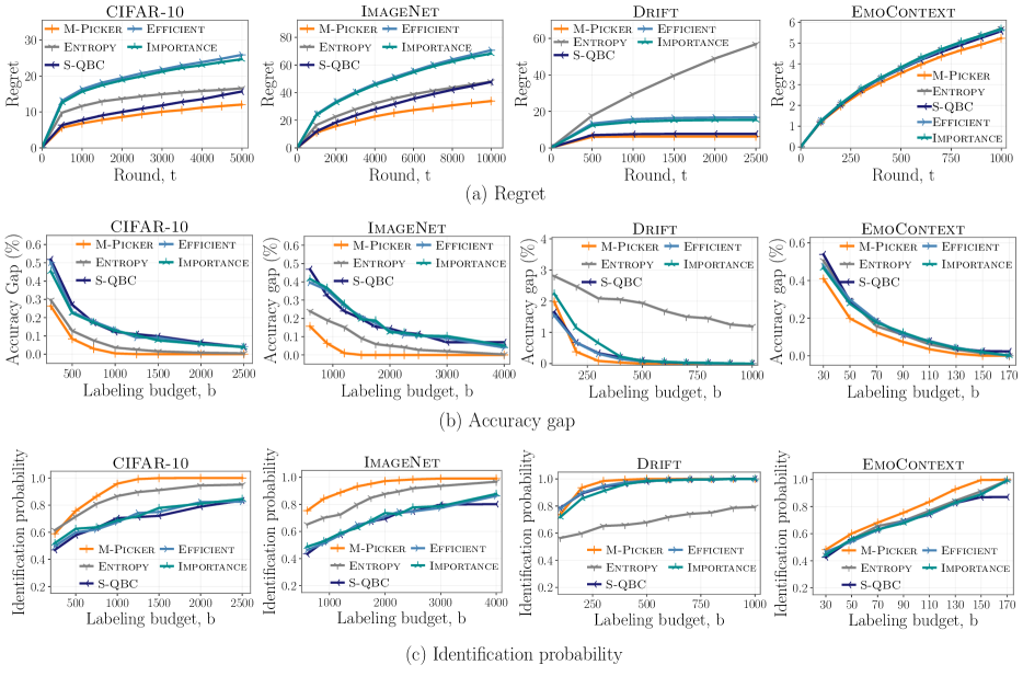
Figure 1: Performance of Model Picker (M-Picker) and other adapted baselines on four datasets {CIFAR-10, ImageNet, Drift, EmoContext}. Model Picker is able to output the true best model with high probability, while querying up to 2.6$\times$ fewer labels than the best competing method.

We conduct an extensive set of experiments to demonstrate the practical performance of Model Picker for online model selection and sequential label prediction. We first run experiments on common data sets where the instances come i.i.d. from a fixed data distribution. This setting allows us to empirically assess the performance in the stochastic setting. We then consider a more challenging scenario where examples come from a drifting data distribution, which we treat as an adversarial stream.

Datasets and Model Collection

We conduct our experiments using various models trained on common datasets such as the SemEval 2019 dataset (EmoContext) for emotion detection (SemEval, ) and the long-term gas sensor drift dataset (Drift) from the UCI Machine Learning Repository (Vergara, 2012; Vergara et al., 2012) as well as on more complex datasets of natural images such as CIFAR-10 and ImageNet. These datasets cover a wide range of scale: CIFAR-10, EmoContext and Drift are of smaller scale while ImageNet is a large scale dataset. Each dataset consists of a large test set (which we later use to construct streams of examples) and (possibly multiple) training sets. For each dataset, we collect a collection of pre-trained models by training various models on the training sets. We provide a detailed explanation on the characteristics of our model collection in Appendix C.1.

For CIFAR-10, we trained 80 classifiers varying in model, architecture, and parameter settings available on Pytorch Hub. The ensemble contains models having accuracies between 55-92% on a test set consisting of 10 000 CIFAR-10 images. The ImageNet dataset poses a 1 000-class classification problem. We collected 102 image classifiers that are available on TensorFlow Hub. The accuracy of these models is in the range 50-82%. For the test set, we use the whole official test set with 50 000 images. For the EmoContext dataset, we collected 8 pre-trained models that are the development history of a participant in SemEval 2019. The accuracy of the models varies in 88-92% on a test set of size 5 509. Lastly, for the Drift dataset, we trained an SVM classifier on each of 9 batches of gas sensor data that were measured in different months. We use the last batch as a test set, which is of size 3 000. Due to the drift behaviour of sensor data among different time intervals, the accuracy of the models on the test set is relatively low, and lies in 25-60%.

Baselines

To compare with existing selective sampling strategies, we implement variations of QBC, namely, vote entropy (Entropy) and structural QBC (S-QBC) as well as label efficient prediction (Efficient) and importance weighted active learning (Importance), as described below. Typically, these methods follow a coin flipping strategy: upon seeing an instance $x_{t}$, a coin is flipped with a bias $q_{t}$, and the label $t$ is requested if and only if the coin comes up heads.

Label Efficient Prediction/Passive Learning. We implement (Cesa-Bianchi et al., 2005) by querying the label of each round randomly with a fixed probability $q_{t}=\varepsilon$. For a fair comparison, we restrict our interest merely to the data instances in which at least two models disagree, as others are non-informative in the ranking of models. In our evaluation, we set the query probability to $\varepsilon=b/T$ for having an expected number of $b$ queries in a stream of size $T$. Note that our way of setting $\varepsilon$ depends on the whole stream for having comparable results in terms of the number of queries, as we shall drop the non-informative samples first.

QBC/Vote Entropy. We use the method of  Dagan and Engelson (1995) and adapt it to the streaming setting as a disagreement-based selective sampling baseline. Upon seeing each instance, we measure the disagreement between the model predictions to compute the query probability. In our implementation, we consider every pre-trained model as a committee member and use vote entropy as the disagreement measure.

Structural QBC. The (interactive) structural QBC algorithm (Tosh and Dasgupta, 2018) is built upon the QBC principle, and its query probability is specified via the disagreement between competing models that are drawn from a posterior distribution $\bm{\rho}_{t}$. After each new query, the posterior is updated as $\bm{\rho}_{t+1}\propto\bm{\rho}_{t}\exp(-\beta{\bm{\ell}}_{t})$, where $\beta$ is a fixed parameter. In our implementation, at each round $t$, we draw two models $i$ and $j$ from $\bm{\rho}_{t}$ with replacement and set the query probability to be the fraction of disagreement between $i$ and $j$ up to round $t$, that is, $q_{t}=\frac{1}{t}\sum_{s\leq t}\mathbb{I}_{\{\bm{p}_{s,i}\neq\bm{p}_{s,j}\}}$.

Importance Weighted Active Learning. We implemented the importance weighted active learning algorithm introduced by Beygelzimer et al. (2008), as well as its variant for efficient active learning (Beygelzimer et al., 2010, 2011). Among these two adaptations of importance weights, we only focus on the superior (Beygelzimer et al., 2008) in our empirical evaluation and leave the others to Appendix C.2.

It is crucial to note that none of the methods above are tailored for the task of ranking pre-trained models and (except for Cesa-Bianchi et al. (2005)) for sequential label prediction. Yet we consider them as selective sampling baselines; see Appendix C.2 for further discussions about our baselines.

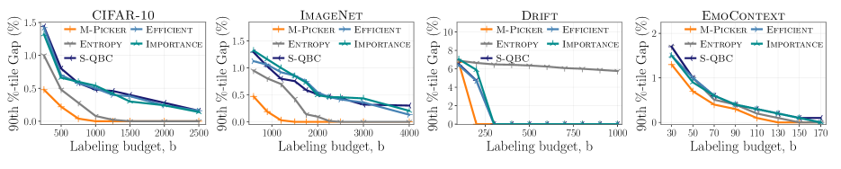
Figure 2: Worst-case analysis on the outputted models: 90th percentile accuracy gap

5.1 Experimental Setup

Evaluation Protocol and Tuning

For a fair comparison, we focus on the following protocol. We sequentially draw $T$ i.i.d. instances uniformly at random from the entire pool of test instances, then input it into each algorithm as a stream, and call it a realization. In each realization, the pre-trained model with the highest accuracy on that stream (considering all labels) is denoted as the true best model of the realization.

For each realization and up to any round $t$, Model Picker outputs $\pi_{t}=\operatorname*{arg\,max}_{i}\bm{w}_{t,i}$ as the best model, and other methods output the model having the highest accuracy on the queried labels. Upon exhausting the stream, we evaluate the performance of each method based on the model that is outputted. We realize this process many times to have an estimate of the expected performance.

For comparing the methods under the same budget constraint, we tune the (hyper-)parameter of each method to query the same number of instances, and compare their average performance under various labeling budgets. For Structural QBC, we treat $\beta$ (in the posterior) as the hyperparameter. For QBC with vote entropy, importance weighted active learning and Model Picker, we introduce a hyperparameter $\beta$ to scale the query probability according to the given labeling budget. Note that by default, Model Picker needs no hyperparameters, and we introduce $\beta$ for the sole reason of fair comparison with other methods. We perform hyperparameter selection via a grid search. The hyperparameters used for each budget, together with a large range of hyperparameters and their respective budgets can be found in Appendix C.4.

Performance Metrics

For a given labeling budget, we consider the following key quantities as performance measures: Regret for a fixed labeling budget, Accuracy gap between the outputted model and the true best model, and Identification Probability, which is the fraction of realizations that methods return the true best model of that realization.

Scaling and Computation Cost

We conduct our experiments on different stream sizes. We choose sizes of 5 000, 10 000, 1 000 and 2 500 for CIFAR-10, ImageNet, EmoContext and Drift test sets, respectively. We implement Model Picker, along with all other baseline methods in Python. All the baseline methods combined, each realization takes between 1 second (for EmoContext) and 4 minutes (for ImageNet) when executed on a single CPU core. Model Picker alone takes between 75 miliseconds (for EmoContext) and 47 seconds (for ImageNet). For all datasets we run 500 independent realizations for each budget constraint. To improve the overall runtime, we run the realizations in parallel over a cluster with 400 cores.

5.2 Experimental Results

We review our numerical results for each of the metrics introduced earlier. We refer to Appendix C.3 for an extensive discussion of our findings. For each of our metrics, we observe the following:

Regret

We measure the regret across all rounds and for those budgets where Model Picker returns the best model with high confidence. Namely, we set the budget to 1 250, 1 200, 130 and 1 000 for the CIFAR-10, ImageNet, EmoContext and Drift datasets, respectively. The regret behaviour is shown in Figure 1(a). In all cases, the regret grows sub-linearly for all algorithms. The regret of our algorithm in all cases is smaller up to a factor of 1.3$\times$, which shows that Model Picker can be used for sequential label prediction tasks as well as model selection.

Accuracy Gap

Next, we consider the average accuracy gap over the realizations. Figure 1(b) shows that the accuracy gaps for Model Picker are much smaller than that of other adapted methods under the same budget constraints. Quantitatively, in both CIFAR-10 and ImageNet datasets, Model Picker achieves the same expected accuracy gap as Entropy by querying nearly 2.5$\times$ less labels. For the Drift dataset, for instance, Model Picker returns a model that is within a 0.1%-neighborhood of the accuracy of best model after querying merely 11% of the entire stream of examples (when the budget is 270 for a stream of size 2 500). Note that active learning over drifting data distribution is a very challenging task, and Efficient (Label Efficient Prediction/Passive Learning) is considered the strongest baseline (Settles, 2009). Our experiments thus suggest that, even for small labeling budgets, Model Picker returns a model whose accuracy is close to that of the best model, if not the best model itself.

Identification Probability

As illustrated in Figure 1(c), Model Picker achieves significant improvements of up to 2.6$\times$ in labeling cost while returning the true best model and requesting far fewer labels than other adapted methods. For CIFAR-10, ImageNet, EmoContext and Drift datasets, Model Picker queries 2.5$\times$, 2.5$\times$, 1.2$\times$ and 1.7$\times$ fewer labels respectively than that of the best competing method (mainly Entropy) to reach confidence levels 95%, 97%, 92% and 97%, respectively. This shows that Model Picker is able to achieve the same identification power as the adapted baselines at a much lower labeling cost.

5.2.1 On the Robustness of Model Picker

Practitioners are often interested in the relative quality of the output model compared to the true best model in a single trial. In this regard, and in the spirit of Theorems 4 and 6, we conduct further numerical analysis on the accuracy of the outputted models over a large number of realizations to investigate if Model Picker performs well with high probability. We compute the 90th percentile of accuracy gap as a proxy for the behaviour of the algorithms in the high probability regime (see Figure 2). In the Drift dataset, for instance, Model Picker returns the true best model after querying merely 8% of the labels (when the budget is 200 with a stream size of 2 500). For the CIFAR-10 and ImageNet datasets, Model Picker returns a model that is within a 0.1%-neighborhood of the accuracy of best model after querying nearly 12% of the entire stream of examples whereas the best competing method achieves this after querying 24% of the same stream of examples. Moreover, Model Picker outputs the true best model after querying 15% and 20% of the entire stream of examples, respectively. These results clearly demonstrate the robustness of Model Picker.

6 CONCLUSIONS

We introduced an online active model selection approach –Model Picker– to selectively query the labels of instances that are informative for ranking pre-trained models and to sequentially predict unseen labels. Our framework is generic, easy to implement, and applies across various classification tasks. We derived theoretical guarantees and illustrate the effectiveness of our method on several real-world datasets.

Acknowledgements

We thank the reviewers for their constructive feedback. This research was supported by the SNSF grant 407540_167212 through the NRP 75 Big Data program and by the European Research Council (ERC) under the European Union’s Horizon 2020 research and innovation programme grant agreement No 815943. CZ and the DS3Lab gratefully acknowledge the support from the Swiss National Science Foundation (Project Number 200021_184628), Innosuisse/SNF BRIDGE Discovery (Project Number 40B2-0_187132), European Union Horizon 2020 Research and Innovation Programme (DAPHNE, 957407), Botnar Research Centre for Child Health, Swiss Data Science Center, Alibaba, Cisco, eBay, Google Focused Research Awards, Oracle Labs, Swisscom, Zurich Insurance, Chinese Scholarship Council, and the Department of Computer Science at ETH Zurich.

 

Online Active Model Selection for Pre-trained Classifiers:
Supplementary Materials

 

[sections] [sections]l1

Appendix A Proofs and Supplementary Lemmas

A.1 On the Choice of Query Probability

Here we elaborate on the discussion for (1). Let $\bm{w}_{t}$ be the current distribution over experts, and $\bm{w}_{t+1}^{(c)}$ be the hypothetical distribution over the experts having observed the loss if the true label is $c$.

First, according to (Narayanan and Rakhlin, 2010, Lemma 1), the divergence $\mathrm{KL}(\bm{w}_{t}\|\bm{w}_{t+1}^{(c)})$ accumulates into the regret. This means that if we do not update $\bm{w}_{t}$ accordingly, we miss this amount of information.

Second, the KL divergence between $\bm{w}_{t}$ and $\bm{w}_{t+1}^{(c)}$ computes

$$\mathrm{KL}(\bm{w}_{t}\|\bm{w}_{t+1}^{(c)})=\eta r+\log(re^{-\eta}+1-r),$$

where $r=\langle\bm{w}_{t},\bm{\ell}_{t}^{c}\rangle$. By Höffdings inequality, one can show that this quantity is between 0 and $\eta^{2}/8$. As the variance is between 0 and $1/4$, it makes sense to scale the KL divergence to the range $[0,1/4]$, by multiplying it by $2/\eta^{2}$. The following lemma completes the comparison promised in Section 4.1. We drop the subscript $t$ for readability.

Lemma 1.

For a distribution over the experts $\bm{w}$ and a fixed $\bm{\ell}\in\{0,1\}^{k}$, define $\bm{w}_{+}\propto\bm{w}\,e^{-\eta\bm{\ell}}$. Then

$$\left\lvert\mathop{\mathrm{Var}}_{A\sim\bm{w}}\bm{\ell}_{A}-\frac{2}{\eta^{2}}\mathrm{KL}(\bm{w}\|\bm{w}_{+})\right\rvert<\frac{1}{18\sqrt{3}}\eta+O(\eta^{2}).$$

Proof.

Define $r=\langle\bm{w},\bm{\ell}\rangle$. We have that

$$\mathrm{KL}(\bm{w}\|\bm{w}_{+})=\eta r+\log(re^{-\eta}+1-r)=\log\operatorname{\mathbb{E}}{e^{-\eta(X-\operatorname{\mathbb{E}}{X})}},$$

where $X$ is a Bernoulli random variable with $\operatorname{\mathbb{E}}{X}=r$. Note that the equation above is the cumulant generating function of $X$ and has the Taylor series

$$\log\operatorname{\mathbb{E}}{e^{-\eta(X-\operatorname{\mathbb{E}}{X})}}=\frac{\eta^{2}}{2}\mathop{\mathrm{Var}}(X)+\frac{\eta^{3}}{6}\kappa_{3}+O(\eta^{4}),$$

where $\kappa_{3}$ is the third cumulant. Note that by the relation between cumulants of a Bernoulli random variable, we have

$$\kappa_{3}=r(1-r)\frac{d}{dr}\kappa_{2}=r(1-r)(1-2r).$$

Easy algebra finds that for $r\in[0,1]$, we have $\kappa_{3}\in[-1/6\sqrt{3},1/6\sqrt{3}]$.

Summing all up, we find

$$\frac{2}{\eta^{2}}\mathrm{KL}(\bm{w}\|\bm{w}_{+})=\mathop{\mathrm{Var}}(X)+\frac{\kappa_{3}}{3}\eta+O(\eta^{2}),$$

and the result of the lemma follows. ∎

A.2 Mix Loss Properties

Define $\widehat{\bm{L}}_{T,*}:=\min_{i\in[k]}\widehat{\bm{L}}_{T,i}$.

Lemma 2.

The cumulative mix loss $M_{T}$ is bounded above by $\widehat{\bm{L}}_{T,*}+\frac{\log k}{\eta_{T}}$.

Before stating the proof, first we bring a standard lemma:

Lemma 3 (de Rooij et al. (2013)).

The cumulative mix loss $M_{T}$ has the following properties for constant learning rates ($\eta_{t}\equiv\eta$ for all $t\geq 1$):

1. $M_{T}=-\frac{1}{\eta}\log\sum_{i\in[k]}e^{-\eta\widehat{\bm{L}}_{T,i}}+\frac{1}{\eta}\log k$,

2. $M_{T}\leq\widehat{\bm{L}}_{T,*}+\frac{1}{\eta}\log k$.

Moreover, for any sequence of decaying learning rates $\{\eta_{t}\}_{t\geq 1}$, let $M_{T}(\{\eta_{t}\})$ be the corresponding cumulative mix loss, and set $M_{T}(\eta_{T})$ be the cumulative mix loss for fixed learning rate $\eta_{T}$. Then, it holds that $M_{T}(\{\eta_{t}\})\leq M_{T}(\eta_{T})$.

Proof.

Define $W_{t}=\sum_{i\in[k]}e^{-\eta\widehat{\bm{L}}_{t,i}}$. For part (i) observe that

$$\langle\bm{w}_{t},e^{-\eta\hat{\bm{\ell}}_{t}}\rangle=\sum_{i\in[k]}\frac{e^{-\eta\widehat{\bm{L}}_{t-1,i}}}{W_{t-1}}e^{-\eta\hat{\bm{\ell}}_{t,i}}=\frac{W_{t}}{W_{t-1}}.$$

Hence, $\log\langle\bm{w}_{t},e^{-\eta\hat{\bm{\ell}}_{t}}\rangle=-\eta m_{t}=\log W_{t}-\log W_{t-1}$, and $M_{T}=\frac{1}{\eta}(\log W_{0}-\log W_{T})$. Observing that $W_{0}=k$ gives (i).

Noticing that $W_{T}\geq e^{-\eta\widehat{\bm{L}}_{T,*}}$ easily implies (ii).

For the last part of the lemma, first we prove that $M_{T}$ for constant learning rate $\eta$ is nonincreasing in $\eta$. This is shown by looking at the derivative of $M_{T}$ with respect to $\eta$ which is equal to

$$\tfrac{1}{\eta^{2}}\log\sum_{i\in[k]}e^{-\eta\widehat{\bm{L}}_{T,i}}-\frac{1}{\eta}\frac{\sum\widehat{\bm{L}}_{T,i}e^{-\eta\widehat{\bm{L}}_{T,i}}}{\sum e^{-\eta\widehat{\bm{L}}_{T,i}}}-\tfrac{1}{\eta^{2}}\log k\leq 0,$$

as $\log\sum_{i\in[k]}e^{-\eta\widehat{\bm{L}}_{T,i}}\leq\log k$.

Now we can prove the last part of the lemma.

$$\sum_{t=1}^{T}m_{t}(\{\eta_{t}\})=\sum_{t=1}^{T}M_{t}(\eta_{t})-M_{t-1}(\eta_{t})\leq\sum_{t=1}^{T}M_{t}(\eta_{t})-M_{t-1}(\eta_{t-1})\leq M_{T}(\eta_{T}).\qed$$

Proof of Lemma 2.

By the lemma above, we see that $M_{T}\leq M_{T}(\eta_{T})\leq\widehat{\bm{L}}_{T,*}+\frac{\log k}{\eta_{T}},$ where we lower bounded the sum over the models by the one that corresponds to $\widehat{\bm{L}}_{T,*}$. ∎

A.3 Lemmas for Regret Bound

Lemma 4.

For any $\eta>0$ it holds that

$$\operatorname{\mathbb{E}}\left[\log\langle\bm{w}_{t},e^{-\eta\hat{\bm{\ell}}_{t}}\rangle+\eta\langle\bm{w}_{t},\hat{\bm{\ell}}_{t}\rangle\right]\leq\eta^{2}.$$

Proof.

If the predictions are all the same, there is nothing to prove, as $\hat{\bm{\ell}}_{t}\equiv 0$ and the expectation vanishes.

Let $\bm{w}_{c}=\sum_{i:\bm{p}_{t}(i)=c}\bm{w}_{t,i}$ and set $c^{*}$ to be the true label of this round. We can then rewrite $q_{t}$ as $q_{t}=\max_{c\in\mathcal{C}}\bm{w}_{c}(1-\bm{w}_{c})\vee\eta$. Observe that

$$\log\langle\bm{w}_{t},e^{-\eta\hat{\bm{\ell}}_{t}}\rangle=\log\left[(1-\bm{w}_{c^{*}})\exp\left\{-\tfrac{\eta}{q_{t}}Q_{t}\right\}+\bm{w}_{c^{*}}\right].$$

It is clear that $\operatorname{\mathbb{E}}{\langle\bm{w}_{t},\hat{\bm{\ell}}_{t}\rangle}=\langle\bm{w}_{t},\ell_{t}\rangle=1-\bm{w}_{c^{*}}$. Hence, the expected value in the lemma is equal to

$$\eta(1-\bm{w}_{c^{*}})+q_{t}\cdot\log\left[(1-\bm{w}_{c^{*}})\exp\left\{-\eta/q_{t}\right\}+\bm{w}_{c^{*}}\right].$$ (2)

Our desired result follows from Lemma 5 by setting $x=1-\bm{w}_{c^{*}}$ and noticing that $q_{t}\geq\bm{w}_{c^{*}}(1-\bm{w}_{c^{*}})\vee\eta$. ∎

Lemma 5.

For all $x\in(0,1)$ and all $\eta\in(0,1]$, defining $u=x(1-x)\vee\eta$, one has

$$f(x,u,\eta):=\eta x+u\log\left[x\,e^{-\frac{\eta}{u}}+1-x\right]\leq\eta^{2}.$$

Moreover, for fixed $x$ and $\eta$, $f(x,u,\eta)$ is decreasing in $u$ for $u\geq\eta$.

Proof.

Note that the value of the LHS and RHS agree when $\eta=0$, so we have to prove that for all $\eta\geq 0$, the derivative of the LHS is at most $\eta$. Fix some $x\in[0,1)$. We prove this fact in two cases:

Case where $\eta\leq x(1-x)$. In this case, $u=x(1-x)$. For brevity, define $y:=\frac{\eta}{x(1-x)}$. The derivative of $f$ with respect to $\eta$ becomes

$$\frac{(e^{y}-1)x(1-x)}{e^{y}(1-x)+x},$$

and we are left with proving

$$\frac{(e^{y}-1)}{e^{y}(1-x)+x}\leq 2y$$

As $0<y\leq 1$, we have that $1+y+y^{2}/2\leq e^{y}\leq 1+y+(e-2)y^{2}$. Replacing these bounds in the equation above leaves us with proving that

$$\frac{1+(e-2)y}{1+(y+y^{2}/2)(1-x)}\leq 2.$$

For a fixed $y$, the left hand side is increasing in $x$, and hence, it is enough to prove that

$$1+(e-2)y\leq 2,$$

but this is true as $y\leq 1$ and $e-1<2$. Thus, we are done with the proof of this case.

Case where $\eta>x(1-x)$. In this case, $u=\eta$, and $f(x,\eta)=\eta x+\eta\log\left[xe^{-1}+1-x\right]$. To prove the claim, we have to show that $x+\log\left[xe^{-1}+1-x\right]\leq\eta$, or, as the left hand side does not depend on $\eta$, we shall prove

$$x+\log\left[xe^{-1}+1-x\right]\leq x(1-x),$$

or, equivalently,

$$1-(1-e^{-1})x\leq e^{-x^{2}},$$

which is proven in Lemma 6. Thus, in both cases, we have proved our inequality and we are done with the proof of the first part of lemma.

We now prove the monotonicity of $f$ with respect to $u$. For that, we show the derivative of $f$ with respect to $u$ is nonpositive. The derivative computes

$$f^{\prime}(u)=\log\left[xe^{-\eta/u}+1-x\right]+\frac{xe^{-\eta/u}\eta/u}{xe^{-\eta/u}+1-x}.$$

Define $a=\eta/u$. The equation above is zero for $a=0$. So it suffices to show that the derivative of above is nonpositive for $0\leq a\leq 1$. Computing the derivative w.r.t. $a$ and setting it less than 0 is equivalent to

$$xe^{-a}+1-x-xe^{-a}\geq 0,$$

which is true. Hence, we are done. ∎

Lemma 6.

For all $x\in[0,1]$ one has $1-(1-e^{-1})x\leq\exp\{-x^{2}\}$.

Proof.

Note that $\exp(-x^{2})$ is concave on $[0,\sqrt{1/2}]$ and convex on $[\sqrt{1/2},1]$. Also at $x=0$ and $x=1$, both sides are equal. Hence, we just have to show that at $x=\sqrt{1/2}$, the right hand side is bigger than the left hand side, which automatically shows the inequality for $x\in[0,\sqrt{1/2}]$, and we have to show that the derivative of the right hand side is smaller than the left hand side at $x=1$, which automatically shows the inequality for the other half of the interval, as $\exp(-x^{2})$ is convex there. For the first part, evaluate

$$\exp(-1/2)-1+(1-1/e)\sqrt{1/2}=(1-1/\sqrt{e})\left(\frac{1}{\sqrt{2}}(1+\frac{1}{\sqrt{e}})-1\right)\geq 0.$$

For the second part, note that $\frac{d}{dx}\exp(-x^{2})=-2x\exp(-x^{2})$, and at $x=1$ it is equal to

$$-2/e\leq-(1-1/e),$$

as $3/e>1$. Hence, we are done. ∎

A.4 Proof of Theorem 2

Proof.

We assume that at all rounds we have $q_{t}>0$, as there is no label request on the rounds that all models predict the same. First observe that

$$\operatorname{\mathbb{E}}{\sum_{t=1}^{T}Q_{t}}\leq\operatorname{\mathbb{E}}\left\{\sum_{t=1}^{T}\eta_{t}+\textstyle\sum_{c\in C}\bm{w}_{t,c}(1-\bm{w}_{t,c})\right\},$$

as maximum of positive numbers is less than their sum. Next, at round $t$ suppose that the true label is $c_{t}$. As $x(1-x)$ is concave and $\sum_{c\neq c_{t}}\bm{w}_{t,c}=1-\bm{w}_{t,c_{t}}=\langle\bm{w}_{t},\bm{\ell}_{t}\rangle=:r_{t}$, using Jensen’s inequality we have

$$\sum_{c\in C}\bm{w}_{t,c}(1-\bm{w}_{t,c})$$

$$\hskip 28.45274pt=\bm{w}_{t,c_{t}}(1-\bm{w}_{t,c_{t}})+\sum_{c\neq c_{t}}\bm{w}_{t,c}(1-\bm{w}_{t,c})$$

$$\hskip 28.45274pt\leq\bm{w}_{t,c_{t}}(1-\bm{w}_{t,c_{t}})+(1-\bm{w}_{t,c_{t}})\left(1-\tfrac{1-\bm{w}_{t,c_{t}}}{|C|-1}\right)$$

$$\hskip 28.45274pt=r_{t}\left(2-\tfrac{|C|}{|C|-1}r_{t}\right).$$

Using Jensen now for the concave function $x(2-\tfrac{|C|}{|C|-1}x)$, we get

$$\sum_{t=1}^{T}\sum_{c\in C}\bm{w}_{t,c}(1-\bm{w}_{t,c})\leq T\cdot\left(\tfrac{\sum r_{t}}{T}\right)\left(2-\tfrac{|C|}{|C|-1}\tfrac{\sum r_{t}}{T}\right).$$

Now observe that if the expected total loss of the best model is $L^{*}$, by our regret bound in Theorem 1 we have

$$\operatorname{\mathbb{E}}{\textstyle\sum r_{t}}\leq 2\sqrt{2T\log k}+L^{*}.$$

Also note that for $x\leq\frac{|C|-1}{|C|}$, the function $x(2-\tfrac{|C|}{|C|-1}x)$ is increasing. Hence, for large enough $T$ (as described in the theorem), $\frac{1}{T}\sum r_{t}\leq\frac{|C|-1}{|C|}$, and we have

$$\operatorname{\mathbb{E}}{\sum_{t=1}^{T}\sum_{c\in C}\bm{w}_{t,c}(1-\bm{w}_{t,c})}\leq\left(2\sqrt{2T\log k}+L^{*}\right)\cdot\left(2-\tfrac{|C|}{|C|-1}\left(2\sqrt{2\log k/T}+L^{*}/T\right)\right).$$

Noting that $\sum\eta_{t}\leq\sqrt{2T\log k}$, one obtains the result. ∎

A.5 Proof of Theorem 6

Proof.

First, we remind the following martingale inequality, which is an improved version of McDiarmid’s:

Lemma 7 (Seldin and Lugosi (2017)).

Let $\xi_{1},\ldots,\xi_{T}$ be a martingale difference sequence with respect to the filteration $\{\mathcal{F}_{t}\}_{t\leq T}$, where each $\xi_{t}$ is integrable and bounded. Let $M_{t}:=\sum_{s\leq t}\xi_{s}$ be the associated martingale. Define $\nu_{T}=\sum_{t\leq T}\operatorname{\mathbb{E}}\{\xi_{t}^{2}\mid\mathcal{F}_{t-1}\}$ and $c_{T}=\max_{t\leq T}\xi_{t}$. Then for any $\beta,\nu,c>0$,

$$\operatorname{\mathrm{Pr}}\left\{\left(M_{T}\geq\sqrt{2\nu\beta T}+\frac{1}{3}c\beta T\right)\wedge(\nu_{T}\leq\nu)\wedge(c_{T}\leq c)\right\}\leq e^{-\beta T}.$$

Remember that the weight of model $i$ at the end of round $t$ is proportional to $\exp\{-\eta_{t+1}\widehat{\bm{L}}_{t}\}$. Hence, identifying the best model $i^{*}$ after round $t$ reduces to the fact that $\widehat{\bm{L}}_{t,i^{*}}=\min_{j\in[k]}\widehat{\bm{L}}_{t,j}$. The probability of this event not happening can be bounded by a union bound on the models:

$$\operatorname{\mathrm{Pr}}\{\exists j\neq i^{*}:\widehat{\bm{L}}_{t,i^{*}}\geq\widehat{\bm{L}}_{t,j}\}\leq\sum_{j\neq i^{*}}\operatorname{\mathrm{Pr}}\{\widehat{\bm{L}}_{t,i^{*}}\geq\widehat{\bm{L}}_{t,j}\}=\sum_{j\neq i^{*}}\operatorname{\mathrm{Pr}}\{\widetilde{D}_{t,j}\leq 0\},$$

where we define $\widetilde{D}_{t,j}=\widehat{\bm{L}}_{t,j}-\widehat{\bm{L}}_{t,i^{*}}$. From now on, we focus on a single model $j$ and drop the index $j$ from $\Delta_{j}$ and $\theta_{j}$. Set $d_{t}:=\bm{\ell}_{t,j}-\bm{\ell}_{t,i^{*}}$ and define

$$\xi_{t}:=\Delta-\frac{d_{t}Q_{t}}{q_{t}}.$$

Note that $\operatorname{\mathbb{E}}\{\xi_{t}\mid\mathcal{F}_{t-1}\}=\operatorname{\mathbb{E}}\{\operatorname{\mathbb{E}}\{\xi_{t}\mid\bm{\ell}_{t},\mathcal{F}_{t-1}\}\mid\mathcal{F}_{t-1}\}=0$. Moreover, the following holds:

$$\xi_{t}\leq\Delta+\frac{1}{q_{t}}\leq\Delta+\eta_{t}^{-1},\quad\operatorname{\mathbb{E}}\{\xi_{t}^{2}\mid\mathcal{F}_{t-1}\}=\operatorname{\mathbb{E}}\left\{\tfrac{d_{t}^{2}}{q_{t}}\mid\mathcal{F}_{t-1}\right\}-\Delta^{2}\leq\theta\eta_{t}^{-1}-\Delta^{2}.$$

The sum of the conditional variances up to $T$ satisfies

$$\sum_{t=1}^{T}\operatorname{\mathbb{E}}\{\xi_{t}^{2}\mid\mathcal{F}_{t-1}\}\leq T\eta_{T}^{-1}\theta-T\Delta^{2}=:\nu$$

Also, set $c=\Delta+\eta_{T}^{-1}$. By lemma above we have

$$\operatorname{\mathrm{Pr}}\left\{\widetilde{D}_{T,j}=\sum_{t=1}^{T}\frac{d_{t}Q_{t}}{q_{t}}\leq T\Delta-\sqrt{2T\nu\beta}-\tfrac{1}{3}c\beta T\right\}\leq e^{-\beta T}.$$

We will find the largest $\beta$ such that the right hand side of the inequality above becomes positive. As it is a quadratic polynomial in $\sqrt{\beta}$, we should have that

$$\sqrt{\beta}\leq\frac{\sqrt{2\nu/T+\frac{4}{3}c\Delta}-\sqrt{2\nu/T}}{\frac{2}{3}c}.$$

Now we lower bound the right hand side, and write $\gamma:=\eta_{T}^{-1}$ for brevity:

$$\frac{\sqrt{2\nu/T+\frac{4}{3}c\Delta}-\sqrt{2\nu/T}}{\frac{2}{3}c} \geq\frac{4\Delta\sqrt{2\nu/T}}{8\nu/T+\frac{4}{3}c\Delta} \text{as }\sqrt{x+a}-\sqrt{x}\geq\frac{2a\sqrt{x}}{4x+a}$$

$$=\frac{3\Delta\sqrt{2\nu/T}}{6\nu/T+c\Delta}$$

$$=\frac{3\Delta\sqrt{2(\gamma\theta-\Delta^{2})}}{6\gamma\theta-5\Delta^{2}+\gamma\Delta}$$

$$=\frac{3\sqrt{2}}{\sqrt{\gamma}}\frac{\Delta\sqrt{\theta-\Delta^{2}/\gamma}}{6\theta+\Delta-5\Delta^{2}/\gamma}$$

$$\geq\frac{3}{\sqrt{\gamma}}\frac{\Delta\sqrt{\theta}}{7\theta} \text{as }\theta\geq\Delta\text{ and }\Delta^{2}/\gamma\leq\theta/2.$$

Hence, we conclude that setting

$$\beta=0.18\sqrt{\log k}\frac{1}{\sqrt{2T}}\frac{\Delta^{2}}{\theta}$$

gives the desired property. The proof follows by plugging in the value of $\beta$ and taking a union bound over the experts. ∎

A.6 Proof of Theorem 4

The proof is very much similar to Theorem 6. The difference is that the conditional variance is bounded above by

$$\operatorname{\mathbb{E}}\{\xi_{t}^{2}\mid\mathcal{F}_{t-1}\}\leq\eta_{t}^{-1}-\Delta^{2},$$

and the rest of the proof follows by setting $\theta=1$.

A.7 Proof of Theorem 3

The first bound is standard and can be found in (Slivkins, 2019). The argument is completed by noting that the expected accuracy gap will be bounded by

$$\frac{1}{T}\operatorname{\mathbb{E}}[\bm{L}_{T,I_{\tau}}-\bm{L}_{T,i^{*}}]\leq\sqrt{\frac{8\log k}{T}},$$

and setting the right hand side less than $\varepsilon$.

For the second part, we use Theorem 4. With probability at most $k\cdot e^{-0.18\Delta^{2}\sqrt{T\log k}}$ the recommended expert is not the best, for which its accuracy gap is at most 1, and otherwise, the best expert is returned, with accuracy gap 0. Combining the two gives the result.

A.8 Proof of Theorem 7

The proof is very similar to Theorem 3, with the difference that here one upper bounds the accuracy gap by $\max_{i}\Delta_{i}$ instead of 1.

A.9 Proof of Theorem 8

First we prove a lemma that help us proving the theorem:

Lemma 8.

The expected number of times that the recommendation $\pi_{t}$ is not the best model is a constant up to any round and is bounded by $\frac{62k}{\lambda^{2}\log k}.$

Proof.

By Theorem 6, we know that the probability of not recommending the best model at round $t$ is upper bounded by $k\cdot e^{-0.18\lambda\sqrt{T\log k}}$. Using integral approximation, one finds that $\sum_{t=1}^{\infty}e^{-a\sqrt{t}}\leq 2/a^{2}$ for all $a>0$. This gives

$$\operatorname{\mathbb{E}}\left[\sum_{t=1}^{\infty}\mathbb{I}_{\{\pi_{t}\neq i^{*}\}}\right]=\sum_{t=1}^{\infty}\operatorname{\mathrm{Pr}}\{\pi_{t}\neq i^{*}\}\leq\sum_{t=1}^{\infty}k\cdot e^{-0.18\lambda\sqrt{T\log k}}\leq\frac{62k}{\lambda^{2}\log k}.\qed$$

Using the lemma, over $T$ rounds, we make at most $\frac{62k}{\lambda^{2}\log k}$ mistakes, for which we get at most $\max_{i}\Delta_{i}$ added to the regret, and in other rounds, we make no mistakes, hence no regrets on those rounds. Adding up gives the result.

Appendix B Example for Large Number of Updates

Consider a binary classification scenario with two models. Set the loss sequence to be $(1,0),(0,1),(1,0),\ldots$, that is, on the odd rounds the second model is correct and on the even rounds, the first one. One can see that the probability of querying the label is always $\bm{w}_{t,1}\bm{w}_{t,2}\vee\eta_{t}$ for all $t$. Hence, this probability is always near $1/4$, as the models weights are always around $1/2$. Hence, the total number of queries is linear.

Appendix C Experiments

C.1 Details on the Model Collections

• CIFAR-10: As an image classification dataset, we train 80 models on CIFAR-10 dataset varying in machine learning models (ranging from DenseNet, Resnet to VGG), architecture and parameter setting. The ensemble of models have accuracies between 55-92% on a test set consists of 10 000 instances.

• ImageNet: This dataset consists of 102 image classification models (ranging from ResNet, Inception to MobileNet) pre-trained on ImageNet that are available on TensorFlow Hub. The accuracy of models occupy the range in 50-80%. For each model, we obtain the ImageNet validation dataset with 50 000 data examples, and furthermore normalize and resize them according to expected input format for each model, and finally conduct inference on the given model to produce predicted labels.

Table 1: Datasets characteristics

Dataset	#Classes	#Instances	#Models	Accuracy of Models
CIFAR-10	10	10 000	80	55-92%
ImageNet	1 000	50 000	102	50-80%
Drift	6	3 000	9	25-60%
EmoContext	4	5 509	8	88-92%
CIFAR-10 (worse models)	10	10 000	80	40-70%

• Drift: For the Drift dataset, we trained models on the gas sensor drift data that is collected over a course of three years. The dataset has ten batches, each collected in different months. We trained an SVM classifier on each of the batch but the last one, and use the last batch of size 3 000 as test set. Although each model has good training accuracy on the batch it is trained on, namely above 90%, their accuracy on the test set lies in 25-60%. This is due to the drift behaviour of sensor data among different time intervals.

• EmoContext: This dataset consist of pretrained models that are the development history of a participant on EmoContexttask in SemEval 2019. The task aims to detect emotions from text leveraging contextual information which is deemed challenging due to the lack of facial expressions and voice modulations. We treat each development as an individual pretrained model where development stages differ in various word representations including ELMo Peters et al. (2018) and GloVe Pennington et al. (2014). The dataset consists of 8 pre-trained models whose accuracy varies between 88-92% on the test set of size 5 509.

• CIFAR-10 V2: We also train a set of models with relatively lower accuracies on CIFAR-10 and call it CIFAR-10 V2. The sole purpose behind creating such a collection is to investigate the performance of Model Picker on a practical scenario like this. Using similar model architectures to that of CIFAR-10, the pretrained models have accuracy between 40-70% on a test set of size 10 000.

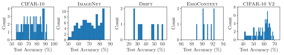
Figure 3: Counts of model accuracies

The properties of model collections for all datasets are depicted in Table 1 on page 1 and Figure 3.

C.2 Note on the Baselines

In this section, we provide further details on some of the adapted baseline methods, namely, query by committee (Entropy), importance weighted active learning (Importance) and efficient active learning (Efal).

• Query by Committee: As indicated in Section 5, we adapt the query-by-committee paradigm proposed in Dagan and Engelson (1995) for model selection in the online setting. The query by committee method consist of two sub-strategies (a) ensemble learning, and (b) determining a maximal disagreement measure. The ensemble learning indicates how the committee is formed from the candidate classifiers. This step is crucial to make the disagreement measure more reliable while aiming to form a set of classifiers with high accuracy. In literature, there exist many ensemble learning methods including Abe and Mamitsuka (1998); Melville and Mooney (2004); Breiman (1996); Freund and Schapire (1995). Most, if not all, of these methods are either designed for pool-based sampling or for cases where observed data is stored. Bagging predictors Breiman (1996) proposes to improve performance of a single predictor by forming a committee from multiple versions of it, where the versions are trained on the bootstrap replicates of training data. This is followed by Abe and Mamitsuka (1998) where diverse ensembles are generated using bagging and boosting techniques previously introduced by Freund and Schapire (1995). These strategies focus on a setting where the observed data is stored as opposed to our setting. Another popular ensemble learning algorithm, Active-Decorate relies on the existence of artificial training data to form a diverse set of examples. In our setting, however, we assume neither storing of previously seen data nor availability of artificial data. In the online setting, however, one could benefit from the strategy introduced in Freund and Schapire (1995). Upon seeing the label $c_{t}$, the authors propose to update the belief on the models such that $\bm{w}_{t}\propto\bm{w}_{t-1}\beta^{\bm{\ell}_{t}}$. We note that, this update rule very closely resembles that of the structural query by committee, which we include in our numerical analysis. In fact, it is identical when both of $\beta$ are tuned to query budget $b$ amount of label in average over many realizations.

  As a disagreement measure, popular choices include vote margin, vote entropy and KL divergence between the label distributions of each committee member and the consensus in Settles and Craven (2008). We first note that the latter two are equivalent for 0-1 loss functions $\ell$. The former, vote margin is measured by the difference between the votes of most voted and second most voted label. We omit this in our analysis motivated by the preliminary observation on the success of entropy over the vote margin.

• Importance Weighted Active Learning: As indicated earlier, we implement the importance weighted active learning algorithm, introduced by Beygelzimer et al. (2008). Formally, upon seeing a new instance $x_{t}$, the algorithm computes a rejection threshold $\theta_{t}$ using sample complexity bounds, and update the hypothesis space $\mathcal{H}_{t}$ to contain only the models whose weighted error is $\theta_{t}$ greater than weighted error of the current best model at time $t$. The sampling probability $q_{t}$ is set to $\max_{i,j\in\mathcal{H}_{t},c\in[C]}{\bm{\ell}}^{(c)}_{t,i}-\bm{\ell}^{(c)}_{t,j}$. We use 0-1 loss. Therefore, adaptation in our setting becomes making query decision based merely on the disagreement between the surviving hypotheses at time $t$. That is, we query the label $c_{t}$ if and only if the surviving classifiers at time $t$ disagree on the labeling of $x_{t}$.

• Efficient Active Learning: We adapt the efficient active learning algorithm presented by Beygelzimer et al. (2010, 2011). In a manner similar to the importance weighted approach, the efficient active learning algorithm also uses the importance weighted framework. Upon receiving a new instance $x_{t}$, the algorithm measures the weighted error estimate between two competing models, and specifies a sampling probability based on a threshold that is a function of $\frac{C_{0}\log t}{t-1}$ for some parameter $C_{0}>0$. If the gap between the estimated weighted errors of two competing models are below this threshold, then the label $c_{t}$ is queried. Otherwise, the algorithm computes the sampling probability $q_{t}$ that is roughly $\min\big{\{}1,\mathcal{O}({1}/{G_{k}^{2}}+{1}/{G_{k}})\frac{C_{0}\log k}{k-1}\big{\}}$ where $G_{k}=\min_{i\in[k]}\bm{L}_{t,i}-\min_{j\in[k],j\neq i}\bm{L}_{t,j}$. We refer to Algorithm 1 of Beygelzimer et al. (2010) for further details. In our implementation, we consider the threshold parameter $C_{0}$ as hyperparameter and tune for efficient active learning algorithm to request amount of labels not exceeding the labelling budget $b$. However, as indicated in Figure 4, it underperforms the importance weighted active learning algorithm. However, it is crucial to emphasize again that these methods are meant to improve supervised training of classifiers instead of ranking of pretrained models. We include them in our comparison for the completeness.

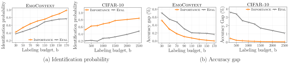
Figure 4: Comparison of importance weighted methods {Importance, Efal} and on the EmoContext and CIFAR-10 datasets

C.3 Performance of Model Picker on models with low accuracies

As mentioned in Section 5, we conduct another numerical analysis on the performance of Model Picker when pretrained models have relatively lower accuracies. Towards that, we train 80 models on CIFAR-10 varying in machine learning models and parameters. The accuracy of pretrained models line in 40-70$\%$ over a test set of of size 10 000. We compare the model selection methods over this new model collection by following the exact same procedure as in the Section 5. We use a stream size of 5 000 and average the results over 500 realizations. Figure 5 summarize the comparison. When the accuracy of pre-trained models are low, the query by committee algorithm expectedly underperforms as the disagreement measure becomes noisy under the existence of models with low accuracies. Model Picker, on the other hand, noticeably outperforms in returning the true best model as well as the ranking of the models (Figure 5). The regret analysis in Figure 5 suggests that the structural query by committee method maintains a low regret throughout the streaming process as well as for different labeling budgets, and very closely followed by Model Picker.

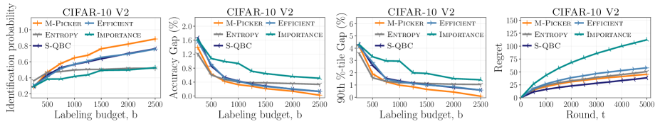
Figure 5: Performance evaluation of model selection methods on CIFAR-10 V2 dataset that consist of pre-trained models with low accuracies.

C.4 Hyperparameters

The hyperparameter tuning is performed via grid search. For each grid point, we run the experiment for 100 realizations and compute the average number of requests. The grid search was performed over the following search space:

• CIFAR-10: Model Picker: [0, 3 000], Entropy: [0, 20], S-QBC: [0, 10], Importance: [0, 0.9], Efal: [0, 1.5e-2]

• ImageNet: Model Picker: [0, 135], Entropy: [0, 22], S-QBC: [0, 20], Importance: [0, 1]

• Drift: Model Picker: [0, 60], Entropy: [0, 4], S-QBC: [0, 4], Importance: [0, 05]

• EmoContext: Model Picker: [0, 60], Entropy: [0, 4], S-QBC: [0, 4], Importance: [0, 05], Efal: [0, 1e-2]

• CIFAR-10 V2: Model Picker: [0, 1 000], Entropy: [0, 3], S-QBC: [0, 10], Importance: [0, 0.9], Efal: [0, 1e-1]

with grid size of 250 where grid points are equally spaced. The respective number of requests for each grid point can be found in our publicly available repository.

Remark that the amount of requests by Model Picker saturates when Model Picker reaches at a high identification probability. Therefore, the update probability is upscaled with a very high value such that Model Picker queries large number of labels, and thus comparison to other methods for large budget constraints are made possible. Practically, this would not be required as Model Picker itself decides when to stop requesting labels. For example, when the update probability is upscaled by a factor of 11 for CIFAR-10 V2 dataset, the number of requests made by Model Picker is 3 800 labels, whereas an upscaling of 835 is used to enable Model Picker requests nearly 4 800 labels.

References

- Abe and Mamitsuka (1998) Naoki Abe and Hiroshi Mamitsuka. Query learning strategies using boosting and bagging. In Proceedings of the Fifteenth International Conference on Machine Learning, ICML 1998, page 1–9, San Francisco, CA, USA, 1998. Morgan Kaufmann Publishers Inc. ISBN 1558605568.
- Ali et al. (2014) Alnur Ali, Rich Caruana, and Ashish Kapoor. Active learning with model selection. In Proceedings of the Twenty-Eighth AAAI Conference on Artificial Intelligence, AAAI’14, page 1673–1679. AAAI Press, 2014.
- Altschuler and Talwar (2018) Jason Altschuler and Kunal Talwar. Online learning over a finite action set with limited switching. In Conference On Learning Theory, pages 1569–1573, 2018.
- Auer et al. (2002) Peter Auer, Nicolo Cesa-Bianchi, and Paul Fischer. Finite-time analysis of the multiarmed bandit problem. Machine learning, 47(2-3):235–256, 2002.
- Bach (2007) Francis R. Bach. Active learning for misspecified generalized linear models. In Advances in Neural Information Processing Systems 19, pages 65–72. MIT Press, 2007.
- Balcan et al. (2009) Maria-Florina Balcan, Alina Beygelzimer, and John Langford. Agnostic active learning. Journal of Computer and System Sciences, 75(1):78–89, 2009.
- Beygelzimer et al. (2008) Alina Beygelzimer, Sanjoy Dasgupta, and John Langford. Importance weighted active learning. ACM International Conference Proceeding Series, 382, 12 2008. doi: 10.1145/1553374.1553381.
- Beygelzimer et al. (2010) Alina Beygelzimer, Daniel J Hsu, John Langford, and Tong Zhang. Agnostic active learning without constraints. In Advances in Neural Information Processing Systems 23, pages 199–207. Curran Associates, Inc., 2010.
- Beygelzimer et al. (2011) Alina Beygelzimer, Daniel Hsu, Nikos Karampatziakis, John Langford, and Tong Zhang. Efficient active learning. In Proceedings of the 28th International Conference on Machine Learning, 2011.
- Breiman (1996) Leo Breiman. Bagging predictors. Machine learning, 24(2):123–140, 1996.
- Cesa-Bianchi et al. (1997) Nicolo Cesa-Bianchi, Yoav Freund, David Haussler, David P Helmbold, Robert E Schapire, and Manfred K Warmuth. How to use expert advice. Journal of the ACM (JACM), 44(3):427–485, 1997.
- Cesa-Bianchi et al. (2005) Nicolo Cesa-Bianchi, Gábor Lugosi, and Gilles Stoltz. Minimizing regret with label efficient prediction. IEEE Transactions on Information Theory, 51(6):2152–2162, 2005.
- Cohn et al. (1994) David A. Cohn, Les E. Atlas, and Richard E. Ladner. Improving generalization with active learning. Machine Learning, 15(2):201–221, 1994.
- Dagan and Engelson (1995) Ido Dagan and Sean P. Engelson. Committee-based sampling for training probabilistic classifiers. In Machine Learning Proceedings 1995, pages 150–157. Elsevier, 1995.
- Dasgupta et al. (2008) Sanjoy Dasgupta, Daniel J Hsu, and Claire Monteleoni. A general agnostic active learning algorithm. In Advances in Neural Information Processing Systems 20, pages 353–360. Curran Associates, Inc., 2008.
- de Rooij et al. (2013) Steven de Rooij, Tim van Erven, Peter D. Grünwald, and Wouter M. Koolen. Follow the Leader If You Can, Hedge If You Must. arXiv:1301.0534 [cs, stat], 2013.
- Freund and Schapire (1995) Yoav Freund and Robert E Schapire. A desicion-theoretic generalization of on-line learning and an application to boosting. In European conference on computational learning theory, pages 23–37. Springer, 1995.
- Gardner et al. (2015) Jacob Gardner, Gustavo Malkomes, Roman Garnett, Kilian Q Weinberger, Dennis Barbour, and John P Cunningham. Bayesian active model selection with an application to automated audiometry. In Advances in Neural Information Processing Systems 28, pages 2386–2394. Curran Associates, Inc., 2015.
- Hazan (2019) Elad Hazan. Introduction to online convex optimization. arXiv preprint arXiv:1909.05207, 2019.
- Karimi et al. (2019) Mohammad Reza Karimi, Andreas Krause, Silvio Lattanzi, and Sergei Vassilvtiskii. Consistent online optimization: Convex and submodular. In Proceedings of Machine Learning Research, volume 89 of Proceedings of Machine Learning Research, pages 2241–2250. PMLR, 16–18 Apr 2019.
- Katariya et al. (2012) Namit Katariya, Arun Iyer, and Sunita Sarawagi. Active evaluation of classifiers on large datasets. In 2012 IEEE 12th International Conference on Data Mining, pages 329–338. IEEE, 2012.
- Kumar and Raj (2018) Anurag Kumar and Bhiksha Raj. Classifier risk estimation under limited labeling resources. In Advances in Knowledge Discovery and Data Mining, pages 3–15, Cham, 2018. Springer International Publishing. ISBN 978-3-319-93034-3.
- Leite and Brazdil (2010) Rui Leite and Pavel Brazdil. Active testing strategy to predict the best classification algorithm via sampling and metalearning. In Proceedings of the 2010 Conference on ECAI 2010: 19th European Conference on Artificial Intelligence, page 309–314, NLD, 2010. IOS Press. ISBN 9781607506058.
- Littlestone and Warmuth (1994) Nick Littlestone and Manfred K Warmuth. The Weighted Majority Algorithm. Elsevier, 1994.
- Madani et al. (2004) Omid Madani, Daniel J. Lizotte, and Russell Greiner. Active model selection. In Proceedings of the 20th Conference on Uncertainty in Artificial Intelligence, UAI ’04, page 357–365, Arlington, Virginia, USA, 2004. AUAI Press. ISBN 0974903906.
- McCallum and Nigam (1998) Andrew McCallum and Kamal Nigam. Employing em and pool-based active learning for text classification. In Proceedings of the Fifteenth International Conference on Machine Learning, ICML ’98, page 350–358, San Francisco, CA, USA, 1998. Morgan Kaufmann Publishers Inc. ISBN 1558605568.
- Melville and Mooney (2004) Prem Melville and Raymond J. Mooney. Diverse ensembles for active learning. In Proceedings of the Twenty-First International Conference on Machine Learning, ICML ’04, page 74, New York, NY, USA, 2004. Association for Computing Machinery. ISBN 1581138385.
- Narayanan and Rakhlin (2010) Hariharan Narayanan and Alexander Rakhlin. Random walk approach to regret minimization. In Advances in Neural Information Processing Systems, pages 1777–1785, 2010.
- Pennington et al. (2014) Jeffrey Pennington, Richard Socher, and Christopher Manning. Glove: Global vectors for word representation. In Proceedings of the 2014 Conference on Empirical Methods in Natural Language Processing (EMNLP), pages 1532–1543, Doha, Qatar, 2014. Association for Computational Linguistics.
- Peters et al. (2018) Matthew Peters, Mark Neumann, Mohit Iyyer, Matt Gardner, Christopher Clark, Kenton Lee, and Luke Zettlemoyer. Deep contextualized word representations. In Proceedings of the 2018 Conference of the North American Chapter of the Association for Computational Linguistics: Human Language Technologies, Volume 1 (Long Papers), pages 2227–2237, New Orleans, Louisiana, 2018. Association for Computational Linguistics. doi: 10.18653/v1/N18-1202.
- Sawade et al. (2010) Christoph Sawade, Niels Landwehr, Steffen Bickel, and Tobias Scheffer. Active risk estimation. In Proceedings of the 27th International Conference on International Conference on Machine Learning, ICML’10, page 951–958, Madison, WI, USA, 2010. Omnipress. ISBN 9781605589077.
- Sawade et al. (2012) Christoph Sawade, Niels Landwehr, and Tobias Scheffer. Active comparison of prediction models. In Advances in Neural Information Processing Systems 25, pages 1754–1762. Curran Associates, Inc., 2012.
- Seldin and Lugosi (2017) Yevgeny Seldin and Gábor Lugosi. An Improved Parametrization and Analysis of the EXP3++ Algorithm for Stochastic and Adversarial Bandits. arXiv:1702.06103 [cs, stat], 2017.
- (34) SemEval, 2019. URL https://www.humanizing-ai.com/emocontext.html.
- Settles (2009) Burr Settles. Active learning literature survey. Technical report, University of Wisconsin-Madison Department of Computer Sciences, 2009.
- Settles and Craven (2008) Burr Settles and Mark Craven. An analysis of active learning strategies for sequence labeling tasks. In Proceedings of the Conference on Empirical Methods in Natural Language Processing, EMNLP ’08, page 1070–1079, USA, 2008. Association for Computational Linguistics.
- Seung et al. (1992) H Sebastian Seung, Manfred Opper, and Haim Sompolinsky. Query by committee. In Proceedings of the fifth annual workshop on Computational learning theory, pages 287–294, 1992.
- Slivkins (2019) Aleksandrs Slivkins. Introduction to Multi-Armed Bandits. arXiv:1904.07272 [cs, stat], September 2019.
- Sugiyama (2006) Masashi Sugiyama. Active learning for misspecified models. In Advances in Neural Information Processing Systems 18, pages 1305–1312. MIT Press, 2006.
- Tosh and Dasgupta (2018) Christopher Tosh and Sanjoy Dasgupta. Interactive structure learning with structural query-by-committee. In Advances in Neural Information Processing Systems 31, pages 1121–1131. Curran Associates, Inc., 2018.
- Vergara (2012) Alexander Vergara. UCI machine learning repository, 2012. URL http://archive.ics.uci.edu/ml/datasets/Gas+Sensor+Array+Drift+Dataset.
- Vergara et al. (2012) Alexander Vergara, Shankar Vembu, Tuba Ayhan, Margaret A Ryan, Margie L Homer, and Ramón Huerta. Chemical gas sensor drift compensation using classifier ensembles. Sensors and Actuators B: Chemical, 166:320–329, 2012.
- Zhang and Chaudhuri (2014) Chicheng Zhang and Kamalika Chaudhuri. Beyond disagreement-based agnostic active learning. In Advances in Neural Information Processing Systems 27, pages 442–450. Curran Associates, Inc., 2014.
- Zhu et al. (2007) Xingquan Zhu, Peng Zhang, Xiaodong Lin, and Yong Shi. Active learning from data streams. In Seventh IEEE International Conference on Data Mining (ICDM 2007), pages 757–762. IEEE, 2007.