Free Energy of a Knotted Polymer Confined to Narrow Cylindrical and Conical Channels

Abstract

Monte Carlo simulations are used to study the conformational behavior of a semiflexible polymer confined to cylindrical and conical channels. The channels are sufficiently narrow that the conditions for the Odijk regime are marginally satisfied. For cylindrical confinement, we examine polymers with a single knot of topology $3_{1}$, $4_{1}$, or $5_{1}$, as well as unknotted polymers that are capable of forming S-loops. We measure the variation of the free energy $F$ with the end-to-end polymer extension length $X$ and examine the effect of varying the polymer topology, persistence length $P$ and cylinder diameter $D$ on the free energy functions. Similarly, we characterize the behavior of the knot span along the channel. We find that increasing the knot complexity increases the typical size of the knot. In the regime of low $X$, where the knot/S-loop size is large, the conformational behavior is independent of polymer topology. In addition, the scaling properties of the free energy and knot span are in agreement with predictions from a theoretical model constructed using known properties of interacting polymers in the Odijk regime. We also examine the variation of $F$ with position of a knot in conical channels for various values of the cone angle $\alpha$. The free energy decreases as the knot moves in a direction where the cone widens, and it also decreases with increasing $\alpha$ and with increasing knot complexity. The behavior is in agreement with predictions from a theoretical model in which the dominant contribution to the change in $F$ is the change in the size of the hairpins as the knot moves to the wider region of the channel.

I Introduction

In recent years, numerous experimental studies have contributed to the systematic investigation of the physical behavior of single DNA molecules confined to nanochannels.Dai et al. (2016); Reisner et al. (2012) Enabled by advances in nanofabrication techniques, such work is mainly motivated by a variety of applications that exploit the effects of confinement on polymers, including DNA sorting,Dorfman et al. (2012) DNA denaturation mapping,Reisner et al. (2010); Marie et al. (2013) and genome mapping.Lam et al. (2012); Hastie et al. (2013); Dorfman (2013); Müller and Westerlund (2017) The development of nanofluidic devices for such purposes naturally benefits from a deep understanding of the conformational statistics and dynamics of polymers in nanochannels.

One aspect of DNA that has received considerable attention in recent years is its propensity to form knots.Orlandini (2017) Knots can occur in DNA as byproducts of various biological processes, including replication, transcription and recombination.Orlandini (2017) Confinement of DNA can dramatically increase the probability and complexity of knot formation, as observed for example in knots in DNA extracted from viruses.Arsuaga et al. (2005) Knots in DNA stretched by elongational fields or confinement in channels have been observed and their dynamics characterized in a variety of in vitro experiments,Rybenkov et al. (1993); Bao et al. (2003); Ercolini et al. (2007); Tang et al. (2011); Renner and Doyle (2015); Plesa et al. (2016); Klotz et al. (2017); Soh et al. (2018a); Amin et al. (2018); Sharma et al. (2019); Klotz et al. (2018); Soh et al. (2018b); Metzler et al. (2006); Reifenberger et al. (2015); Amin et al. (2018); Ma and Dorfman (2020) where they are typically detected by the presence of bright spots in optical images of stained DNA molecules. Knots can be created by a variety of methods, including tying individual DNA molecules using optical tweezersBao et al. (2003) or by application of a strong alternating electric field in microfluidics devices that employ elongational fields.Tang et al. (2011)

Of particular relevance to the present work are those experiments which have examined knotted DNA confined to nanochannels.Metzler et al. (2006); Reifenberger et al. (2015); Amin et al. (2018); Ma and Dorfman (2020) Understanding such systems is important for the development of next-generation genomics technology that use nanochannel mapping assays, where the presence of knots or backfolds introduces artifacts that may lead to erroneous results.Reifenberger et al. (2015) Several years ago, Reifenberger et al. examined “topological events” occurring along DNA molecules driven into narrow square channels (40–50 nm wide) using an analysis of spikes in the YOYO intensity profile.Reifenberger et al. (2015) The presence of either backfolds or knots was evident from intensity spikes of approximately 3$\times$ that of the adjacent region. It was noted that frequency of these structures was significantly less and their size significantly greater than the values predicted from simulations.Micheletti and Orlandini (2014); Jain and Dorfman (2017) In another recent study, Amin et al. developed a nanofluidic “knot factory” which utilizes hydrodynamic compression of single DNA molecules against a barrier in wide (325 nm$\times$414 nm) rectangular nanochannels to form sequences of simple knots that can be studied upon subsequent extension of the molecule.Amin et al. (2018) They found that the knotting probability increases with chain compression and with waiting time in the compressed state. They also noted a breakdown of Poisson statistics of knotting probability at high compression, likely due to interactions between knots. Very recently, Ma and Dorfman used the technique of Ref. Amin et al., 2018 for knot generation to study diffusion of knots in nanochannels in the extended de Gennes regime.Ma and Dorfman (2020) They observed a subdiffusive motion, contradicting the prevailing theory for diffusion of knots in channel-confined DNA, but consistent with earlier observations of self-reptation of knots for unconfined DNA under tension. Note that the mechanisms used to create knots in such experiments do not allow for selection of knots of a specific type, nor is the knot topology easy to characterize afterward, other than an approximate measurement of the DNA contour length contained in the knot. Indeed, the difficulty in distinguishing a knot from a simple backfold was noted in Ref. Reifenberger et al., 2015.

Numerous computer simulation studies of knotted polymers have contributed to elucidating the behavior of knots in DNA.Micheletti et al. (2011); Orlandini (2017) A number of these studies have examined the statics and dynamics of knotted polymers confined to narrow channels.Mobius et al. (2008); Micheletti and Orlandini (2012); Orlandini and Micheletti (2013); Nakajima and Sakaue (2013); Micheletti and Orlandini (2014); Suma et al. (2015); Dai et al. (2015a); Jain and Dorfman (2017) Möbius et al. examined the dynamics of a trefoil knot in a channel-confined semiflexible chain in the Odijk regime using Brownian dynamics (BD) simulations together with a coarse-grained theoretical model.Mobius et al. (2008) They concluded that the knot inflates to macroscopic size before untying. As noted elsewhere,Nakajima and Sakaue (2013) however, their theoretical model omits the key feature of excluded-volume interactions between overlapping subchains, which tend to reduce knot size and may lead to knot localization instead of knot expansion. In subsequent Monte Carlo simulation studies, such knot localization of a trefoil knot was observed for both flexibleNakajima and Sakaue (2013); Dai et al. (2015b) and semiflexibleDai et al. (2015a) chains under confinement in channels. In the case of flexible chains, the typical knot size was observed to decrease monotonically with decreasing channel size, and the overall behavior was explained using a model employing the de Gennes blob scaling and repulsion between blobs in different overlapping subchains in the confined knot.Nakajima and Sakaue (2013) For the case of confined semiflexible chains, the typical knot size varied non-monotonically with decreasing channel width, initially increasing, then reaching a maximum before decreasing as the channel becomes narrower.Dai et al. (2015a) This behavior was explained using a theoretical model for the free energy based on an earlier theory of knots in unconfined wormlike polymers.Grosberg and Rabin (2007); Dai et al. (2014, 2015b) Other MC simulation studies have shown that the knotting probability for DNA (with persistence length $\approx 50$ nm) peaks for channel widths slightly below 100 nm, and that simpler knots (especially trefoil) tend to dominate.Micheletti and Orlandini (2012); Orlandini and Micheletti (2013); Jain and Dorfman (2017) Langevin dynamics simulations suggest that the abrupt decrease in the knotting probability for channel widths below 100 nm arises from a decrease in the knot lifetime and an increase in the mean time between the formation of knots for decreasing channel widths in this range.Micheletti and Orlandini (2014); Suma et al. (2015)

In the present study we use MC simulations to examine the behavior of a single knotted semiflexible polymer confined to a narrow channel in the Odijk regime. This regime is defined by the condition that $P\gg D$, where $P$ is the persistence length and $D$ is the channel width, though the condition is only marginally satisfied in this work. With the exception of Ref. Mobius et al., 2008, each of the simulation studies discussed above considered channels that correspond either to the extended de Gennes scaling regime ($P\ll D\ll P^{2}/w$, where $w$ is the polymer width) or else the onset of Odijk scaling for channel widths near 50 nm. Although the equilibrium probabilities of knots in this regime are expected to be very low, it is nevertheless of interest to extend the range of confinement over which knotting behavior is well characterized, as noted in the conclusions of Ref. Amin et al., 2018. In addition, it is convenient for testing theoretical models in such a clearly defined scaling regime. As various studies have noted that simple knots are most probable under channel confinement, we choose to consider only knots of these types. We employ simulation methods similar to those used previously to study polymer folding in nanochannelsPolson et al. (2017); Polson (2018) and measure the variation in the free energy with respect to the extension length, which is closely correlated with the knot size. These measurements are comparable to the measurement of the variation in $F$ with knot length carried out in Ref. Dai et al., 2015a for wider channels.

In addition to confinement to channels of constant cross-sectional area, we also examine confinement of a knotted polymer to a conical channel. Conical confinement of polymers has been the subject of recent experimentalBell et al. (2017) and theoreticalNikoofard et al. (2013); Nikoofard and Fazli (2015); Kumar and Kumar (2018); Polson and Heckbert (2019) work, though to our knowledge the effects of such confinement on knots has not yet been considered. Here, we examine the variation of the free energy with respect to knot position along the channel for a polymer tethered at the narrow end of the cone. For convenience, we also choose cone angles that are sufficiently small for Odijk scaling to hold throughout. The variation of the free energy functions with cone angle and knot complexity can be understood in the context of a theoretical model that is similar in spirit to those developed in Refs. Nakajima and Sakaue, 2013 and Dai et al., 2015a to describe knots in other scaling regimes.

II Model

The simulations examine a semiflexible polymer confined to a long, narrow channel. We model the polymer as a chain of $N$ hard spheres, each with diameter $\sigma$. The pair potential for non-bonded monomers is thus $u_{\rm{nb}}(r)=\infty$ for $r\leq\sigma$ and $u_{\rm{nb}}(r)=0$ for $r>\sigma$, where $r$ is the distance between the centers of the monomers. Pairs of bonded monomers interact with a potential $u_{\rm{b}}(r)=0$ if $0.9\sigma<r<1.1\sigma$ and $u_{\rm{b}}(r)=\infty$, otherwise. Thus, the length of each bond fluctuates slightly about its average value. The bending rigidity of the polymer is modeled using a bending potential with the form, $u_{\rm bend}(\theta)=\kappa(1-\cos\theta)$. The angle $\theta$ is defined for a consecutive triplet of monomers centered at monomer $i$ such that $\cos\theta_{i}=\hat{u}_{i}\cdot\hat{u}_{i+1}$, where $\hat{u}_{i}$ is the unit vector pointing from monomer $i-1$ to monomer $i$. The bending constant $\kappa$ determines the overall stiffness of the polymer and is related to the persistence length $P$ byMicheletti et al. (2011) $\exp(-\langle l_{\rm bond}\rangle/P)=\coth(\kappa/k_{\rm B}T)-k_{\rm B}T/\kappa$. For our model, the mean bond length is $\langle l_{\rm bond}\rangle\approx\sigma$. For sufficiently large $\kappa/k_{\rm B}T\gg 1$ this implies $P/\sigma\approx\kappa/k_{\rm B}T$.

In most simulations, the confining channel is a hard cylindrical tube of uniform diameter $D$. Each monomer interacts with the wall of the cylindrical tube with a potential $u_{\rm w}(r)=0$ for $r<D/2$ and $u_{\rm w}(r)=\infty$ for $r>D/2$, where $r$ is the distance of the monomer center from the central axis of the cylinder. Thus, $D$ is defined to be the diameter of the cylindrical volume accessible to the centers of the monomers and the actual diameter of the cylinder is $D+\sigma$. A second confinement geometry that we examine is a hard conical channel with nonuniform diameter $D(z,\alpha)=D_{0}+2z\tan\alpha$. Here, $z$ is the distance along the channel axis and $\alpha$ is the half-angle of the cone. In this case, we fix one end monomer to position $z$=0, where the diameter is $D(0,\alpha)$=$D_{0}$. The various parameters describing the two model systems are illustrated in Fig. 1.

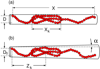
Figure 1: Illustration showing the definition of the various parameters described in the text for a polymer confined to (a) a cylindrical channel and (b) a conical channel. The polymer extension, $X$, and knot span, $X_{\rm k}$ shown in panel (a) are defined exactly the same for the system in panel (b).

In most cases the confined polymer contains a single knot of topology $3_{1}$, $4_{1}$, or $5_{1}$. We also consider the case of an unknotted polymer, for which an S-loop containing two hairpin turns may be present for sufficiently short end-to-end polymer extension length. In order to maintain the knot topology of the polymer we constrain the hairpin turns of the knot or S-loop to lie between the two end monomers along the channel. In effect, the knot or S-loop is constrained to lie between two virtual walls attached to the end monomers that slide along the channel with these monomers. Generally, this feature introduces only very weak artifacts in the free energy and other data, as discussed in Sec. IV.1.

III Methods

Monte Carlo simulations are used to calculate the configurational free energy $F$ of the confined polymer. In the case of a polymer confined to a cylinder, we calculate $F$ as a function of $X$, the end-to-end extension length of the polymer along the channel axis. In addition, we examine the $X$-dependence of the knot span, $X_{\rm k}$, which is defined as the distance measured along the channel between the tips of the two hairpin turns present in the knot or S-loop. For a polymer confined to a conical channel, we measure $F$ as a function of $Z_{\rm k}$, the position of the center of the knot along the channel axis measured with respect to the end monomer fixed at the narrow end of the channel. The quantities $X_{\rm k}$ and $Z_{\rm k}$ are both illustrated in Fig. 1.

To measure the free energy functions, the simulations employed the Metropolis algorithm and the self-consistent histogram (SCH) method.Frenkel and Smit (2002) The SCH method can be used to find the free energy function $F(\lambda)$, where $\lambda$ is any quantity that is a function of the monomer coordinates. In this study, we choose $\lambda$=$X$ for cylindrical confinement and $\lambda$=$Z_{\rm k}$ for conical confinement. To implement the method we carry out many independent simulations, each of which employs a unique “window potential” of the form:

$$W_{i}(\lambda)=\begin{cases}\infty,\hskip 22.76219pt\lambda>\lambda_{i}^{\rm max}\cr 0,\hskip 25.60747pt\lambda_{i}^{\rm min}\leq\lambda\leq\lambda_{i}^{\rm max}\cr\infty,\hskip 22.76219pt\lambda<\lambda_{i}^{\rm min}\end{cases}$$ (1)

where $\lambda_{i}^{\rm min}$ and $\lambda_{i}^{\rm max}$ are the limits that define the range of $\lambda$ for the $i$-th window. Within this range, a probability distribution $p_{i}(\lambda)$ is calculated in the simulation. The window potential width, $\Delta\lambda\equiv\lambda_{i}^{\rm max}-\lambda_{i}^{\rm min}$, is chosen to be sufficiently small that the variation in $F$ does not exceed 2–3 $k_{\rm B}T$. The windows are chosen to overlap with half of the adjacent window, such that $\lambda^{\rm max}_{i}=\lambda^{\rm min}_{i+2}$. The window width was typically $\Delta\lambda=2\sigma$. The SCH algorithm was employed to reconstruct the unbiased distribution, ${\cal P}(\lambda)$ from the $p_{i}(\lambda)$ histograms. The free energy follows from the relation $F(\lambda)=-k_{\rm B}T\ln{\cal P}(\lambda)$. A detailed description of the implementation of the SCH algorithm for a polymer system comparable to that studied here is presented in Ref. Polson et al., 2013.

For the case of a knotted polymer confined to a conical channel, calculation of the free energy energy function $F(Z_{\rm k})$ required a more advanced approach than a straightforward application of the multiple-histogram method used for $F(X)$ in the case of cylindrical channels. The problem is due to long correlation times associated with fluctuations in the polymer extension and, correspondingly, in the knot span, $X_{\rm k}$. Typically, the correlation times are comparable to the run time of an entire simulation. The variation of $F$ with $Z_{\rm k}$ was found to depend significantly on the knot span. Consequently, the histogram associated with each window in Eq. (1) are sensitive to the initial values of $X_{\rm k}$, which randomly distributed in the initialization routine. This tended to result in free energy functions of poor quality. To address this problem, we use the multiple-histogram method to measure $F(Z_{\rm k})$ for fixed $X$ (which essentially also fixes the knot span), and then carry out an appropriate average of these functions for a collection of values of $X$. The details of the method are outlined in Appendix A.

Polymer configurations were generated by carrying out single-monomer moves using a combination of translational displacements and crankshaft rotations. In addition, standard reptation moves were also employed for the case of cylindrical confinement. The maximum values of the displacements and rotations are chosen to be small enough to not alter the knot topology of the polymer. Trial moves were accepted with a probability $p_{\rm acc}$=${\rm min}(1,e^{-\Delta E/k_{\rm B}T})$, where $\Delta E$ is the difference in the total energy between trial and current states. Note that $\Delta E$=$\infty$ if any nonbonded monomers overlap, or if the bonding constraints or window potential constraints of Eq. (1) are violated, in which case $p_{\rm acc}=0$ and the move is rejected. Otherwise, $\Delta E$ is simply the difference in the total bending energy. Simulations for polymers confined to a cylinder employed a polymer of length $N$=400 monomers. The calculations of $F(Z_{\rm k})$ for confinement in a conical channel used shorter chains of $N$=200 monomers because of the much larger number of simulations required for each free energy function. Equilibration times were chosen to be sufficiently long to ensure the decay of transients in measured quantities that arise from artificial (though convenient) initial configurations. The system was equilibrated for typically $5\times 10^{6}$ MC cycles, following which a production run of $2\times 10^{8}$ MC cycles was carried out. A MC cycle is defined as a sequence of $N+1$ trial moves, each of which is either a reptation move or else a change in the coordinates of a single randomly selected monomer. The probability of attempting a reptation move was chosen to be equal to that of moving any single monomer. For single-monomer movement, random displacement and rotation are selected with equal probability.

In the simulations we measure both the span and position of the knot or S-loop along the confining channel. This requires identifying the portion of the polymer that is contained within the knot. One option is to compute the Alexander polynomial of the chain after closing both ends by a loop based on the minimally interfering closure scheme.Tubiana et al. (2011) Although this method is widely used in simulation studies of knotted polymers, we have chosen not to adopt this approach in the present study. The central problem is that the calculations of the variation of $F$ with knot position require that the the knot lie within the range of the window defined by the potential of Eq. (1). Consequently, determining whether a MC move is accepted or rejected requires calculation of the knot position each time a move is attempted. The high computational cost of the chain-closure method makes this approach infeasible. Fortunately, the fact that we consider knotted polymers confined to very narrow channels provides a pragmatic alternative. In this regime the knot is characterized by two hairpin turns, and the presence of additional hairpins for polymer contour lengths considered here is extremely improbable. It is straightforward to determine the positions of the monomers at the hairpins with minimal computational cost. We define the span of the knot (or S-loop, in the case of an unknotted polymer) as the distance along the channel between the these two hairpins and its position as the mean position of the hairpins. This approach is similar to that employed by Möbius et al., who studied unknotting kinetics for a polymer confined to a channel under Odijk conditions.Mobius et al. (2008)

For the results presented below, distances are measured in units of $\sigma$ and energies are measured in units of $k_{\rm B}T$.

IV Results

IV.1 Cylindrical channels

We first examine the properties of the free energy function $F(X)$ for polymers confined to a cylindrical channel. Figures 2(a) and (b) show representative functions for an unknotted polymer and a polymer with a single $3_{1}$ knot, respectively. For $X\lesssim 350$, the unknotted polymer is buckled and contains an S-loop. (An S-loop is an unknotted structure containing at least two hairpin turns and three elongated subchains between the hairpins, similar in appearance to the knot structure shown in Fig. 1(a) except for the key difference in topology.) In each case, results are shown for a polymer of length $N$=400, bending rigidity of $\kappa$=15, and confining cylinder diameter of $D$=4. Sample snapshots of the polymer at three different extension lengths identified by the three points labeled in each graph are shown in panels (c) and (d). The free energy functions share common features of (i) the presence of a single minimum at large $X$, (ii) a broad linear regime at lower $X$, and (iii) a steep rise in the free energy at the highest extensions. The slopes of the curves in the linear regime are nearly equal for the two systems.

The key qualitative difference between the functions is the deep free energy well around the minimum present in the case of the unknotted polymer (labeled point B in Fig. 2(a)). The origin and scaling properties of this free energy well have been explained previously.Polson et al. (2017) The extension at the free energy minimum corresponds roughly to the mean extension length for an elongated semiflexible polymer in the Odijk regime, where no backfolding is present. Upon decreasing the end-to-end extension $X$, the polymer buckles and eventually forms two hairpin turns that constitute the S-loop. The depth of the well is a measure of the free energy associated with the formation of the hairpins. Further decreasing $X$ increases the span of the S-loop along the channel, but leaves the hairpins unaffected. The linear increase of $F$ with decreasing $X$ arises from the interactions between the three subchains of the S-loop that lie between the two hairpins. For sufficiently narrow channels the scaling of the free energy gradient in the linear regime, $f\equiv dF/dX$, is expectedOdijk (2008) to scale with $D$ and the persistence length, $P$, according to $f\sim D^{-5/3}P^{-1/3}$, with small deviations in the scaling exponents arising from finite-size effects.Polson et al. (2017); Polson (2018) At higher extensions, where $X>X_{\rm min}$, the rapid increase in $F$ arises from the decrease in entropy associated with the suppression of lateral fluctuations in the conformations sampled by the polymer.

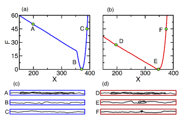
Figure 2: (a) Free energy $F$ vs extension length $X$ for a polymer of length $N=400$ and a bending constant of $\kappa=15$, confined within a cylindrical channel of diameter $D$=$4$. The polymer contains an S-loop in the linear regime. (b) As in panel (a) except for a polymer with a trefoil knot present instead of an S-loop. (c) Sample conformations corresponding to the points labeled in panel (a) for the S-loop. (d) Sample conformations corresponding to the points labeled in panel (b) for the trefoil knot.

Unlike the case for an unknotted polymer, the hairpins present in a knotted polymer are not eliminated when the extension length increases and the polymer unbuckles. Thus, there is no corresponding release of the hairpin free energy (which is mainly the hairpin bending energy for a polymer in the Odijk regime) when an S-loop is removed. Consequently, the deep free energy well associated with the hairpin formation is not present. Obviously, the value of $X_{\rm min}$ is closely connected to both the most probable knot contour length and knot span length. The greater each of these lengths are, the lower the corresponding value of $X_{\rm min}$. As will be examined in detail below, the values of these quantities are each strongly affected by the polymer bending rigidity, the channel diameter, and the topology of the knot. Note that the scaling properties of the free energy for knotted polymers confined to channels have been elucidated in two previous studies;Nakajima and Sakaue (2013); Dai et al. (2015a) however, neither approach is directly applicable to interpreting the present results. Ref. Nakajima and Sakaue, 2013 considered fully-flexible polymers in the de Gennes regime, while Ref. Dai et al., 2015a examined knots in semiflexible polymers, they used channels of width $D\gtrsim P$, which is wider than those considered here. Those studies considered only trefoil knots, and in each of them a metastable knot was observed whose most probable size was dependent on the channel dimension. The underlying factors governing the scaling behavior of the typical size of a trefoil knot in the Odijk regime will be examined later in this section of the article in the analysis of the data of Fig. 6(e) and (f).

Figure 3 shows free energy functions for polymers of length $N$=400 in narrow cylindrical channels with $D$=4. Results are shown for bending rigidities in the range $\kappa=5-15$, and each panel shows functions for a given value of $\kappa$ for unknotted polymers, as well as those with knots with topologies of $3_{1}$, $4_{1}$ and $5_{1}$. In the case of an unknotted polymer, the depth of the free energy well decreases as the polymer becomes more flexible. This is mainly due to the reduction in the hairpin bending energy that is released as the extension $X$ increases and the polymer unbuckles. Indeed, at $\kappa$=5 no free energy well is present, as expected for the regime $D\gtrsim P$ where the concept of a hairpin turn is no longer meaningful. The slope of the curves in the linear regime gradually increases as the polymer rigidity lessens. This is qualitatively consistent with the theoretical prediction that the slope scales as $P^{-1/3}$ in the Odijk regime.Odijk (2008); Polson et al. (2017); Polson (2018) Another notable trend is the overlap in the curves for different topologies at each $\kappa$ in the linear regime. This overlap is not perfect, but close enough to suggest that polymer knot topology does not strongly affect the overall conformational behavior of the knot/S-loop when that structure has a sufficiently large span along the channel. As a clarifying example, the conformational behavior illustrated in the snapshots of state A in Fig. 2(c) for an S-loop and state D in Fig. 2(d) for a $3_{1}$ knot are, by this measure, very similar. As $X$ increases, the free energy curve for each knotted polymer eventually peels away from the S-loop curve. Generally, the value of $X_{\rm min}$ for each knot topology decreases with increasing complexity of the knot. Thus, the most probable contour length and knot span increases with knot complexity.

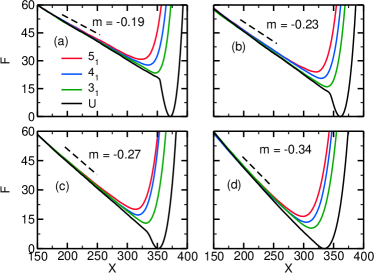
Figure 3: Free energy $F$ vs extension length $X$ for both knotted polymers ($3_{1}$, $4_{1}$, and $5_{1}$) and unknotted polymers that may contain an S-loop (U). The polymers are of length $N$=400 and are confined to a cylindrical channel with a diameter of $D$=4. Results are shown for (a) $\kappa$=$15$, (b) $\kappa$=$10$, (c) $\kappa$=7.5, and (d) $\kappa$=5. In each panel, the slope $m$ obtained obtained for a fit to the linear portion of $F$ for the S-loop is labeled.

Figure 4 shows free energy functions for a polymer of length $N$=400 with a fixed bending rigidity of $\kappa$=15. Results are shown for cylinder diameters ranging from $D=4-7$ for each of the topologies considered in Fig. 3. Again, we note the approximate overlap in the linear regime between the curves for knots with different topologies. As before, this suggests that knots and S-loops have similar conformational behavior in the case where these structures are sufficiently large. The value of the slope decreases with increasing channel width. This is qualitatively consistent with the expectation that the slope scales as $D^{-5/3}$ in the Odijk regime.Polson et al. (2017); Polson (2018) As this slope lessens with increasing $D$, there is a widening in the distribution of extension lengths resulting from an increase in the probability of shorter extension lengths. This corresponds to a widening of the knot size distribution through an increase in the probability of larger knots. This is qualitatively consistent with the trend observed in simulations of Jain and Dorfman for knotted polymers in square channels for confinement near the onset of Odijk scaling (i.e. $D\approx P$).Jain and Dorfman (2017) As in Fig. 3, $X_{\rm min}$ decreases as the complexity of the knot topology increases. Thus, the most probable contour length and span of the knot increases with knot complexity.

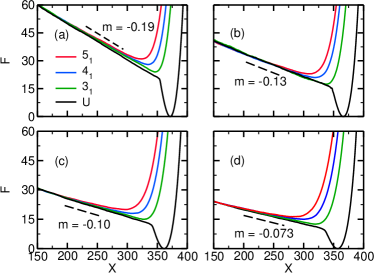
Figure 4: Free energy functions for knotted polymers ($3_{1}$, $4_{1}$, and $5_{1}$) and unknotted polymers that may contain an S-loop (U). Each polymer has a length of $N$=400 and a bending rigidity of $\kappa$=15. Results are shown for (a)$D$=4, (b) $D$=5, (c) $D$=6, and (d) $D$=7.

As noted in Sec. II, the knot or S-loop is artificially constrained to lie completely between the two ends of the polymer. This feature was incorporated into the model to prevent the polymer knot from untying or changing to a different knot type. This artificial confinement is expected to reduce the entropy of the system and thus increase the free energy. Here, we estimate the effect on the free energy functions by modeling the knot as a particle undergoing a 1-D random walk along the channel. For a channel of constant cross-sectional area, the energy is independent of the knot position. Neglecting fluctuations in the span of the knot, the range of positions accessible to its center is $X-X_{\rm k}$. Thus, the entropy is $S_{\rm c}/k_{\rm B}=\ln(X-X_{\rm k})+{\rm const.}$, and the free energy is $F_{\rm c}/k_{\rm B}T=-S_{\rm c}/k_{\rm B}=-\ln(X-X_{\rm k})+{\rm const.}$ Note that the knot span $X_{\rm k}$ depends on $X$, $D$ and $\kappa$, but is insensitive to knot topology for extensions in the linear regime of the free energy (i.e. $X$ is sufficiently less than $X_{\rm min}$).

To test this approximation, we calculate $F(X)$ for an “ideal” polymer, by which we mean that monomer-monomer overlap is permitted. Note that the topology of the polymer will not be preserved in the simulation, but this is not expected to matter for $F_{\rm c}$. Figure 5(a) shows the free energy function $F_{\rm id}$ for an ideal polymer with $N$=400, $D$=4 and $\kappa$=15. As expected, $F_{\rm id}$ does not display the steep increase with decreasing $X$ seen in Fig. 3(a) for a “real” polymer system (i.e. where no monomer-monomer overlap is permitted) with otherwise the same conditions. However, there is a residual small increase in $F$ with decreasing $X$ resulting from the artificial confinement described above. Overlaid on this curve is the estimate of $F_{\rm c}$. We see excellent agreement between the two results in the regime where the two hairpins are present (i.e. $X<350$). The corrected free energy, $F_{\rm id}^{*}\equiv F_{\rm id}-F_{\rm c}$ is now independent of polymer extension, demonstrating the validity of the approximation. Figure 5(b) shows free energy functions $F(X)$ and corrected free energy functions, $F^{*}(X)$, where the latter are calculated as in Fig. 5(a). The correction leads to a small but significant change in the curves. Specifically, it slightly decreases the free energy gradient in the linear regime and extends the range of $X$ over which the curves remain linear.

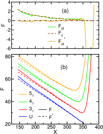
Figure 5: (a) Illustration of the effect of artificial longitudinal confinement of the knot/S-loop on the free energy. $F_{\rm id}$ is the free energy function of an ideal polymer (i.e. overlap of monomers is permitted) for $N$=400, $D$=4, and $\kappa$=15. The longitudinal confinement free energy is defined: $F_{\rm c}\equiv-\ln(X-X_{\rm k})+{\rm constant}$, where $X_{\rm k}=X_{\rm k}(X)$ is the knot span. The shifted free energy is $F^{*}_{\rm id}\equiv F_{\rm id}-F_{\rm c}$. (b) Free energy for real polymers (i.e. no overlap between monomers). Note that $F^{*}\equiv F-F_{\rm c}$. The polymer has either a knot or an S-loop. As in (a), $N$=400, $D$=4, and $\kappa$=15.

The variation of $X_{\rm min}$ for the free energies of Figs. 3 and 4 with $\kappa$ and $D$ for both knotted and unknotted polymers is shown in Fig. 6(a) and (b), respectively. As expected, the Odijk prediction for the mean extension length, which is overlaid on the data, agrees well with the results for the unknotted polymer, particularly at large $\kappa$ and low $D$. To quantify the shift in $X_{\rm min}$ of the knotted polymers relative to that of the unknotted polymer, we define $\Delta X_{\rm min}\equiv X_{\rm min}(n_{1})-X_{\rm min}(U)$, where $X_{\rm min}(n_{1})$ is the extension length at the free energy minimum for a polymer with a knot of topology $n_{1}$ for $n$=3, 4, and 5, and $X_{\rm min}(U)$ is the corresponding extension length of an unknotted polymer. $\Delta X_{\rm min}$ a measure of the reduction in the extension length of the polymer caused by the presence of the knot and is roughly proportional to the contour length of the knot. Figures 6(c) and (d) shows the variation of $\Delta X_{\rm min}$ with $\kappa$ and $D$, respectively. A clearer measure of knot size is $X_{\rm k}^{*}$, span of the knot along the channel evaluated at the free energy minimum, $X=X_{\rm min}$. The knot span is defined as the distance measured along the channel between the tips of the two hairpins in the knot. Figures 6(e) and (f) show the variation of $X_{\rm k}^{*}$ with $\kappa$ and $D$, respectively. As expected, the general trends for $\Delta X_{\rm min}$ are the same as for $X_{\rm k}^{*}$, since both are measures of knot size. For each measure of knot size, three main trends are apparent. First, $\Delta X_{\rm min}$ and $X_{\rm k}^{*}$ increase with both the polymer rigidity and the channel diameter. Second, the rate of increase of each with $\kappa$ and $D$ appears to increase with increasing knot complexity. Finally, for any given value $\kappa$ and $D$, $\Delta X_{\rm min}$ and $X_{\rm k}^{*}$ increases with knot complexity. An increase in knot size with knot complexity for elongated polymers was also observed in the case of an unconfined knotted polymer under tension,Caraglio et al. (2015) as well as for polymers confined to channels somewhat wider than those examined here (i.e. $D\approx P$).Jain and Dorfman (2017) However, the increase in knot size with increasing $D$ differs from the behavior observed in Ref. Jain and Dorfman, 2017, where it remained relatively unchanged.

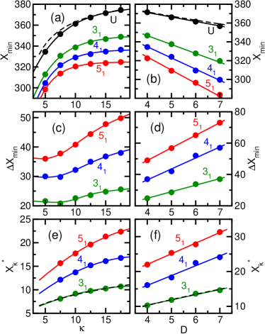
Figure 6: (a) Extension length at the free energy minimum $X_{\rm min}$ vs bending rigidity $\kappa$ for a polymer of length $N$=400 in a tube of diameter $D$=4. Results are shown for unknotted (U) polymers and polymers with a single knot of $3_{1}$, $4_{1}$ and $5_{1}$ topology. The solid lines are guides for the eye. The dashed line is the Odijk prediction for the equilibrium extension length. (b) As in (a), except $X_{\rm min}$ vs $D$ for polymer bending rigidity of $\kappa$=15. (c) $\Delta X_{\rm min}$ vs bending rigidity $\kappa$ for $D$=4, where $\Delta X_{\rm min}$ is defined in the text. (d) As in (c), except $\Delta X_{\rm min}$ vs $D$ for polymer bending rigidity of $\kappa$=15. (e) Knot span $X_{\rm k}^{*}$ at $X=X_{\rm min}$ vs $\kappa$ for $D$=4. (f) Knot span $X_{\rm k}^{*}$ at $X=X_{\rm min}$ vs $D$ for $\kappa$=15. The dashed black lines in panels (e) and (f) are the functions $1.65D^{2/3}P^{1/3}$ for fixed $D$=4 and $P$=15, respectively.

What factors determine the most probable knot span? The rapid rise in $F$ at high $X$ corresponds mainly to the loss in entropy associated with the suppression lateral conformational fluctuations. In addition, increasing $X$ in the linear regime ($X<X_{\rm min}$) leads to a reduction in knot size. For a sufficiently large knot this reduces excluded volume interactions between deflection segments in the knot and causes the decrease in $F$. These two contributions to $F$ alone guarantee the presence of a minimum. Now consider further the intra-knot excluded volume interactions. The predictionOdijk (2008) and subsequent verification by computer simulationPolson et al. (2017) that the free energy gradient of an S-loop approximately scales as $f\equiv dF/dX\sim D^{-5/3}P^{-1/3}$ is derived by modeling the polymer as a collection of equivalent hard cylinders. The cylinders have a length given by the Odijk deflection length $l_{d}\sim D^{2/3}P^{1/3}$ and inter-cylinder interactions are estimated using the second-virial approximation. In this picture, increasing $X$ corresponds to shortening the knot and removing these virtual hard cylinders out of the knot into a region where no such interactions are present. Thus, $F$ decreases. Eventually, however, when the knot span is of the order of $l_{\rm d}$, this picture breaks down. The strands between the hairpins are (obviously) connected to the hairpins. These constraints are expected to severely constrain the orientational freedom of the (effectively rigid) strands, in a manner that the orientational entropy sharply drops with shortening knot span. Thus, it is expected that when $X_{\rm k}\approx l_{\rm d}$ a contribution to the free energy emerges that steeply rises with increasing $X$, leading to a minimum in the free energy.

The simple argument above suggests that $X_{\rm k}^{*}\approx l_{\rm d}$. The dashed curves in panels (e) and (f) of Fig. 6 are plots of $1.65D^{2/3}P^{1/3}$ for for fixed $D$=4 and $P$=15, respectively. These dashed curves overlap with the $X_{\rm k}^{*}$ perfectly, suggesting this argument is valid for trefoil knots. On the other hand, attempts to fit the data for $4_{1}$ and $5_{1}$ knots using this scaling were not successful. The increased entanglement for elongated knots of greater topological complexity likely introduces additional constraints for those knots that further reduce the orientational freedom of the knot strands. Clearly, this effect kicks in at larger knot span that is not simply a multiple of $l_{\rm d}$. Further elucidation of such effects in a future study would be worthwhile.

Let us now consider the relationship between knot span and polymer extension length. Figure 7(a) shows the variation in the knot span along the channel with the extension length of a polymer with a $3_{1}$ knot. Results are shown for a polymer of bending rigidity $\kappa$=15 and for various channel diameters. The black dotted curves overlaid on the data are corresponding results for the span of an S-loop for an unknotted polymer. Several trends are apparent. As expected, the knot span decreases with increasing $X$. For the range of $X$ corresponding to the linear regime in the free energy functions of Fig. 3, $X_{\rm k}$ decreases linearly with $X$. As $X$ approaches and then passes the extension at minimum free energy, $X_{\rm min}$, the rate of decrease of knot span with $X$ decreases. For any value of $X$, the knot span decreases slightly with increasing channel diameter. However, for each $D$, the curves are essentially parallel with a slope $dX_{\rm k}/dX\approx-0.5$. In the case of an unknotted polymer for extensions where an S-loop is present, the S-loop span is virtually identical to the $3_{1}$ knot span at any $X$.

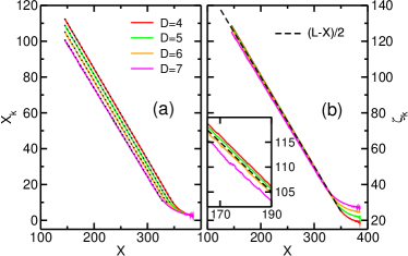
Figure 7: (a) Variation of the extension length of a $3_{1}$ knot with respect to the extension length of a polymer confined to a channel. Results are shown for a polymer of bending rigidity $\kappa$=15 in a channel of various channel diameters. The black dotted lines overlaid on the solid curves are corresponding results for the S-loop extension length for an unknotted polymer. (b) Variation of $\zeta_{\rm k}$ with $X$, where $\zeta_{\rm k}$ is defined by Eq. (3) and calculated using the data for the $3_{1}$ knot in panel (a). The dashed line shows the theoretical prediction that $\zeta_{\rm k}=(L-X)/2$. The inset shows a close-up of the data.

To understand the origin of these trends, we employ the scaling properties of a channel-confined polymer in the Odijk regime. Note that the required condition $D\ll P$ is only marginally satisfied in this case ($P/D=2.14-3.75$), and thus some quantitative discrepancy between the predicted and observed behavior is to be expected. Since the results for knotted ($3_{1}$) and unknotted (S-loop) polymers are identical over the regime of interest ($X<X_{\rm min}$), we ignore the effects of topology. Let us first consider a polymer with no backfolding. Recall that the mean extension length of a polymer in this regime is given by $\bar{L}_{\parallel}=L(1-\alpha_{\parallel}D^{2/3}P^{-2/3})$, where $L$ is the contour length of the polymer and where the prefactor is $\alpha_{\parallel}=0.1701\pm 0.0001$.Dai et al. (2016) Now, consider a polymer with two hairpin folds, which may result from an S-loop or a knot. We first define an effective contour length as $\ell\equiv L-\pi D$ to exclude the contour in the two hairpins. Here, we assume the hairpin diameter is $D$, which is likely only a slight overestimate in the narrow-channel limit.Odijk (2006); Chen (2017) The mean span of the S-loop/knot, ${X}_{\rm k}$, is the mean distance between the two hairpins. We next define the effective extension of the polymer as the sum of the extensions along the channel of all elongated pieces of the polymer, which excludes the hairpins. As explained in the Supplemental Material, the effective extension of the polymer is given by $\ell_{\parallel}=2{X}_{\rm k}+X-2D$. Replacing $L\rightarrow\ell$ and $L_{\parallel}\rightarrow\ell_{\parallel}$ in the relation for $L_{\parallel}$ above, it follows:

$${X}_{\rm k} = -{\textstyle\frac{1}{2}}X+{\textstyle\frac{1}{2}}L-({\textstyle\frac{\pi}{2}}-1)D-{\textstyle\frac{1}{2}}\alpha_{\parallel}L(D/P)^{2/3}$$ (2)

$$+{\textstyle\frac{1}{2}}\alpha_{\parallel}\pi D(D/P)^{2/3}.$$

The first term accounts for the observed slope of $dX_{\rm k}/dX\approx-0.5$, while the third and fourth terms account for the observed decrease in $X_{\rm k}$ with increasing $D$. In our simulations, $\pi D\ll L$, and so the 5th term is negligible relative to the 4th term and can be omitted. In the calculation above, we have neglected the effects of fluctuations in the extension length and interactions between the elongated segments in the knot/S-loop. In the Supplemental Material, we show that these effects are negligible. Defining the shifted knot extension, $\zeta_{\rm k}$, as

$$\zeta_{\rm k} \equiv {X}_{\rm k}+({\textstyle\frac{\pi}{2}}-1)D+{\textstyle\frac{1}{2}}\alpha_{\parallel}LD^{2/3}P^{-2/3},$$ (3)

it follows from Eq. (2) (omitting the negligible 5th term) that $\zeta_{\rm k}=(L-X)/2$ for all values of $D$, $P$, independent of the polymer extension $X$. Figure 7(b) shows that such a shift does lead to near collapse of the data to the predicted curve for $N$=400 in the range of $X$ corresponding to the linear regime of the free energy. The data collapse is slightly worse for the largest channel diameter of $D$=7, where the Odijk regime conditions are least well satisfied. Overall, the data collapse to a universal curve is reasonably good, given the approximations employed in this theoretical model.

IV.2 Conical channels

We now consider the behavior of a knotted polymer in a conical channel. Rather than measuring the free energy with respect to polymer extension we use instead the knot position, $Z_{\rm k}$. The central goal here is to characterize the effects of the varying channel cross-sectional area at the location of the knot as it samples different locations along the channel. As noted in Section III a problem with measuring $F(Z_{\rm k})$ is the very long correlation time associated with the fluctuations in the polymer extension length. Consequently, we choose instead the approach described in Appendix A. Essentially, this involves calculation of $F(Z_{\rm k}|X)$, the variation in the free energy with knot position for fixed polymer extension $X$, and carrying out a suitable average of these functions.

Figure 8(a) shows the variation of $F$ with knot position for a range of polymer extension lengths. Results are shown for a polymer of length $N$=200 and bending rigidity $\kappa=15$ with a $3_{1}$ knot confined to a conical channel with $D_{0}$=4, and cone angle $\alpha$=0.57^∘. The steep rise in $F$ at low and high extremes of $Z_{\rm k}$ is an expected artifact arising from the constraint that the entire span of the knot lie between the two ends of the polymer. (Recall that this constraint is imposed to preserve the knot topology and prevent the knot from untying.) This rapid increase arises when an edge of the knot makes contact with the “virtual wall” attached to an end monomer. This occurs when $|Z_{\rm k}-Z_{\rm end}|\approx X_{\rm k}/2$, where $Z_{\rm end}$ is the position of the end monomer nearest to the knot center. As $X$ increases, the knot span decreases and the knot can occupy a wider range of positions along the channel before it makes contacts with the virtual wall. Thus, as $X$ increases we observe an increase in the distance along the channel between these steep increases in $F$.

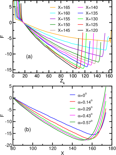
Figure 8: (a) Free energy $F$ vs $Z_{\rm k}$ calculated for a polymer under conical confinement at fixed polymer extension length. The polymer has a length $N=200$, a bending constant of $\kappa=15$, and a localized $3_{1}$ knot along its contour. The cap of the narrow end of the cone has diameter $D_{0}=4$, and the cone angle is $\alpha=0.57^{\circ}$. Results for various cone angles are shown. For visual clarity, the curves are each shifted such that $F$=0 at $Z_{\rm k}$=17.5. (b) Free energy $F$ vs extension length for a polymer with $N=200$, $\kappa=15$, and a $3_{1}$ knot confined to a cone with a cap diameter of $D_{0}=4$. Results for several cone angles are shown.

In the region where the knot is not close to the end monomers, $F$ decreases monotonically as the knot moves in the direction of increasing channel diameter, i.e. increasing $Z_{\rm k}$. In addition, rate of change in $F$ with $Z_{\rm k}$ increases monotonically as the extension length increases. The origin of these trends is straightforward. As the knot moves to a wider part of the channel, the bending energy associated with the hairpin turns decreases, contributing to a decrease in $F$. Another contribution to this trend is the free energy associated with the overlap of the three strands of the polymer inside the knot between the hairpins, which is also expected to decrease as the diameter of the channel decreases. This second contribution to the free energy is proportional to the knot extension length, which decreases as $X$ increases. Consequently, there is a weaker contribution to variation of $F$ with $Z_{\rm k}$, and thus the rate $dF/dZ_{\rm k}$ decreases with increasing extension length.

The method described in Appendix A requires calculation of the $F$ with the polymer extension length $X$ for knotted polymers confined to a conical channel. Results are shown in Fig. 8(b) for the case of a $3_{1}$ knot and for several cone angles. For visual clarity, the curves are shifted so that $F$=0 at $X$=80. The curves are qualitatively similar to those in Figs. 3 and 4. Increasing the cone angle has the effect of increasing the curvature of the functions for $X<X_{\rm min}$ and decreasing the value of $X_{\rm min}$. The latter trend results from the fact that the extension length decreases with increasing $D$ and larger angles correspond to more of the polymer confined to wider parts of the channel.

Using the method described in Appendix A and results such as those shown in Fig. 8, we calculate the variation of the free energy with $Z_{\rm k}$. Figure 9(a) shows $F(Z_{\rm k})$ for several cone angles. Results are shown for a polymer of length $N$=200 and bending rigidity $\kappa$=15 in a cone with an end fixed at a position where the channel diameter is $D_{0}$=4. We consider cones that deviate only slightly from cylindrical channels, with a cone half-angle ranging from $\alpha$=0^∘ (i.e. a cylindrical channel) to $\alpha$=0.57^∘. This range of $\alpha$ is chosen to ensure that the condition for the Odijk regime is satisfied at least marginally for all positions along the channel occupied by the polymer, i.e. $D(z)<P$. The free energy functions are shown in the range $10\leq Z_{\rm k}\leq 130$. Inside this range the free energy is unaffected by the artificial constraint that the entire span of the knot lie between the two end monomers. At either extreme outside this range the knot compresses against the virtual walls connected to these end monomers and the free energy abruptly rises. For visual clarity, the free energy curves are shifted so that $F$=0 at $Z_{\rm k}$=10. Unsurprisingly, the free energy is independent of knot position for cylindrical channels with constant cross-sectional area. However, for $\alpha>0$ the free energy decreases monotonically with increasing $Z_{\rm k}$, i.e., as the knot moves to a channel location with a larger channel diameter. In addition, at any given $Z_{\rm k}$ the decrease in the free energy relative to the $Z_{\rm k}=10$ reference point is larger for larger $\alpha$. Thus, the dependence of $F$ on $Z_{\rm k}$ and $\alpha$ indicates that the knot position probability increases with increasing channel width at the knot location. Figure 9(b) shows free energy functions for three different knots, each for a polymer with $\kappa$=15 and a cone with $D$=4 and $\alpha$=$0.57^{\circ}$. The curves are all qualitatively similar. The key trend is the more rapid decrease in $F$ with $Z_{\rm k}$ for knots of increasing complexity.

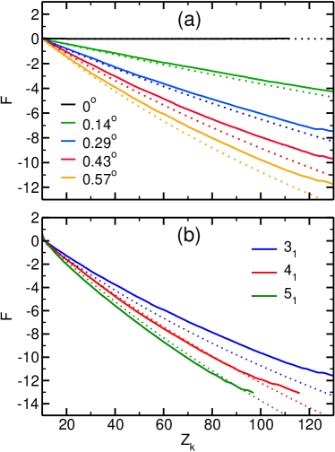
Figure 9: (a) Free energy $F$ vs $Z_{\rm k}$ calculated for a polymer under conical confinement. The polymer has a length $N=200$, a bending constant of $\kappa=15$, and a localized $3_{1}$ knot along its contour. The cap of the narrow end of the cone has diameter $D_{0}=4$. Results for various cone angles are shown. The solid curves are the simulation data and the dashed curves are the predictions using the theory developed in Appendix C. (b) Free energy functions for $N$=200, $\kappa$=15, $D_{0}$=4, and cone angle of $\alpha$=$0.57^{\circ}$. Results are shown for three different knot topologies.

The trends in Fig. 9 can be better understood using a theoretical description that incorporates insights gained from recent theoretical studies of folded polymers under confinement in channels. The theory is developed and described in detail in Appendices B and C. Here, the channel-confined knotted polymer is modeled as a single linear polymer of extension $X$ that overlaps with a ring polymer of extension $X_{\rm k}$, as illustrated in Fig. 10 of Appendix C. The ring polymer is a simple representation of the knot. The lengths of the linear and ring polymer are designed to vary in a manner such that the total length of the two is held fixed. In this context, the free energy has four principal contributions: (1) the free energy associated with the hairpin turns; (2) the overlap free energy of the three subchains in the knot that lie between the two hairpins; (3) the confinement free energy of the extended sections of the ring polymer outside the hairpins; and (4) the confinement free energy of the linear polymer. Figure 11 in Appendix C shows each of the four contributions to $F(Z_{\rm k})$ for the case of $\kappa=15$, $D_{0}=4$ and $\alpha=0.57^{\circ}$. We note that the dominant contribution is the free energy of the hairpins, which accounts for about 70% of the variation of $F$ with knot position. This is mainly a result of the large amount of bending energy stored in the hairpins that is released as the channel widens.

Curves for the theoretical predictions of $F(Z_{\rm k})$ are overlaid on simulation results in Figs. 9(a) and (b). The quantitative accuracy of the predictions is surprisingly good, given the crudeness of the approximations employed in the theory. The key qualitative trends are both reproduced by the theory: (1) $F$ decreases more rapidly with $Z_{\rm k}$ as the cone angle increases and (2) $F$ decreases more rapidly as the knot complexity increases. The first feature is mainly due to the release of the hairpin free energy (mainly bending energy) as the knot moves in the direction of increasing channel width. The second feature appears to be associated with the increase in knot span with knot complexity, as well as the greater rate of change of knot size with channel width for increasing knot complexity, as observed in Fig. 6(d) and (f).

V Conclusions

In this study we have used MC simulations to investigate the properties of the conformational free energy of a knotted semiflexible polymer confined to cylindrical and conical channels. The channels are sufficiently narrow for the conditions for Odijk scaling ($D<P$) to be marginally satisfied. Most other comparable simulation studies of knotted polymers have considered systems with wider channels corresponding either to extended de Gennes scaling regime or else near the onset of Odijk scaling ($D\approx P$). Those cases are more relevant to recent experiments of knotted DNA.Metzler et al. (2006); Reifenberger et al. (2015); Amin et al. (2018); Ma and Dorfman (2020) Our choice to focus on the Odijk regime is motivated by an expectation that future experiments for Odijk-regime systems will eventually be carried out, as well a basic interest in the fundamental physics of the behavior of knots in a regime that has been otherwise so thoroughly examined for polymers in the absence of self-entanglement. This study builds on our recent work of folded semiflexible polymers under confinementPolson et al. (2017); Polson (2018) and employs similar methodology.

For cylindrical channels, we measured the variation of $F$ with the extension length $X$ for polymers with knots of various types, as well as for unknotted polymers. Since the value of $X$ determines the span of the knot, the calculations in effect measure the variation of $F$ with knot size. As in other scaling regimes for both flexibleNakajima and Sakaue (2013) and semi-flexibleDai et al. (2015a) chains, we observe a metastable knot, corresponding to a minimum in $F(X)$. The most probable knot size $X_{\rm k}^{*}$ increases with persistence length $P$, channel width $D$, and knot complexity. For trefoil knots, $X_{\rm k}^{*}$ scales approximately with the Odijk deflection length, though the behavior for more complex knots is less straightforward. For knots in the size regime where $X_{\rm k}>X_{\rm k}^{*}$ (i.e. knots larger than the most probable size) the scaling of $F$ with respect to $X$, $P$ and $D$ is comparable to that for unknotted polymers containing an S-loop. Specifically, in this regime the scaling of free energy gradient is in approximate agreement with the prediction of $f\equiv dF/dX\sim D^{-5/3}P^{-1/3}$ previously derivedOdijk (2008) and confirmedPolson et al. (2017) for the case of an S-loop. In addition, knot span dependence on $X$ and its scaling with $D$ and $P$ is identical to that of an S-loop. We conclude that the overall conformational behavior of knots is very similar to that of an S-loop, at least in the regime where $X_{\rm k}>X_{\rm k}^{*}$.

In addition to cylindrical channels, we also examined the behavior of knots in conical channels. In this case, we measured the variation of $F$ with respect to knot position along the channel, $Z_{\rm k}$. Generally, we find that $F$ decreases as $Z_{\rm k}$ increases, i.e., as the knot moves to the wider part of the channel. The main driving force is the reduction in the hairpin free energy (mainly the hairpin bending energy) with increasing channel diameter, which is unsurprising given the narrowness of the channels in the Odijk regime. Generally, we find that the rate of decrease of $F$ with $Z_{\rm k}$ increases with increasing cone angle and with knot complexity. A simple theoretical model that describes the knotted polymer as a linear polymer overlapping with a ring polymer is able to account for these trends.

One outstanding matter concerns the general criteria that determine the metastable knot size $X_{\rm k}^{*}$ for knots of arbitrary complexity and how $X_{\rm k}^{*}$ scales with respect to channel width and persistence length. A future goal in subsequent work will be to develop a theoretical model for the free energy in the spirit of that developed in Ref. Dai et al., 2015a applicable to the Odijk regime and for arbitrary knot type. The observation that scaling $X_{\rm k}$ matches that of the Odijk deflection length in the case of trefoil knots is a useful starting point. In addition, it will be useful to measure directly the variation of $F$ with $P$ and $D$, as opposed simply to measuring how varying those parameters changes $F(X)$. A thermodynamic integration method such as that employed in Refs. Matthews et al., 2012 and Poier et al., 2014 is well suited for such a measurement. Finally, the effects of channel cross-section shape on the knot behavior would be of interest to examine, as we have done previously in our study on backfolded polymers under confinement in channels.Polson (2018) We hope that experiments on knotted DNA will eventually be carried out to test the predictions of our simulations.

Appendix A Calculation of the free energy for conical confinement

In principle, the multiple-histogram method used to calculate $F(X)$ for knotted polymers in cylinders in Sec. IV.1 can be employed to measure $F(Z_{\rm k})$, the knot-position dependence of the free energy for a polymer under confinement in a cone. However, as noted in Sec. III previously, this approach suffers from the presence of long correlation times associated with fluctuations in the polymer extension and, correspondingly, in the knot extension length, $X_{\rm k}$. Typically, the correlation time is comparable to or greater than the entire simulation run time. Since the variation of $F$ with $Z_{\rm k}$ tends to depend significantly on the knot extension, the contributions to $F$ from the histogram associated with each window potential of Eq. (1) are highly sensitive to the initial values of $X_{\rm k}$. These values tend to be randomly distributed during the initialization routine of the simulations, and so the resulting free energy functions tend to be of poor quality. To circumvent this problem, we employ the multiple-histogram method to measure $F(Z_{\rm k})$ for fixed $X$ (which essentially fixes the knot span), and then carry out an appropriate average of these functions for a number of values of $X$. The algorithm is described below.

Consider a knotted polymer confined to a cone aligned along the $z$ axis with one end monomer tethered to $z$=0. Let $Z_{\rm k}$ and $X$ be the knot position along $z$ and the polymer extension length, respectively. The probability distribution for the knot position, $\mbox{$\cal{P}$}(Z_{\rm k})$, satisfies

$$\mbox{$\cal{P}$}(Z_{\rm k})=\int\mbox{$\cal{P}$}(Z_{\rm k}|X)\mbox{$\cal{P}$}(X)dX,$$ (4)

where $\mbox{$\cal{P}$}(X)$ is the probability distribution for the polymer extension, and where $\mbox{$\cal{P}$}(Z_{\rm k}|X)$ is the conditional probability for the knot position for a given extension length $X$. Here, the integral is over all accessible values of $X$. Each probability distribution is related to a corresponding free energy function; that is,

$$\mbox{$\cal{P}$}(X) = \frac{\exp\left(-\beta F(X)\right)}{\int dX\,\exp\left(-\beta F(X)\right)},$$ (5)

$$\mbox{$\cal{P}$}(Z_{\rm k}) = \frac{\exp\left(-\beta F(Z_{\rm k})\right)}{\int dZ_{\rm k}\exp\left(-\beta F(Z_{\rm k})\right)},$$ (6)

and

$$\mbox{$\cal{P}$}(Z_{\rm k}|X) = \frac{\exp\left(-\beta F(Z_{\rm k}|X)\right)}{\int dZ_{\rm k}\,\exp\left(-\beta F(Z_{\rm k}|X)\right)},$$ (7)

where $\beta\equiv 1/k_{\rm B}T$. It follows from Eqs. (4) – (7) that:

$$\beta F(Z_{\rm k})=-\ln\left[\int dX\,C(X)\exp\left(-\beta(F(Z_{\rm k}|X)+F(X))\right)\right],$$

(8)

where

$$C(X)\equiv\left[\int\exp(-\beta F(Z_{\rm k}|X))\,dZ_{\rm k}\right]^{-1}.$$ (9)

We use Eq. (8) to calculate the dependence of the free energy on knot position in the simulations. To do so, the free energy function $F(X)$ is calculated for a polymer in a cone using the same method as that employed for cylindrical channels in Section IV.1. The free energy function $F(Z_{\rm k}|X)$ is calculated by constraining the extension length to a particular value $X$ and then employing the multiple-histogram method described in Section III to calculate the probability distribution for the knot position, $Z_{\rm k}$. The integrals of Eqs. (8) and (9) are approximated with discrete summations; thus,

$$\beta F(Z_{\rm k})\approx-\ln\left[\sum_{i}C(X_{i})\exp\left(-\beta(F(Z_{\rm k}|X_{i})+F(X_{i}))\right)\right],$$

(10)

where

$$C(X_{i})\equiv\left[\sum_{Z_{\rm k}}\exp(-\beta F(Z_{\rm k}|X_{i}))\right]^{-1}.$$ (11)

The values of $X_{i}$ are chosen to lie between bounds defined such that $F(X_{i})-F_{\rm min}<7k_{\rm B}T$, where $F_{\rm min}$ is the minimum of the free energy function. The probability that $X$ lies outside this range is negligible. Typically we choose 10–15 values of $X_{i}$ within this range.

Appendix B Confinement free energy of a polymer in cone in the Odijk regime

A theoretical estimate for the variation of the free energy of a knotted polymer with respect to knot position is provided in Appendix C. The theoretical model used requires the confinement free energy of an unknotted polymer under conical confinement, which we derive in this appendix.

Consider a polymer confined to a conical channel of half-angle $\alpha$ aligned along the $z$-axis. One end monomer is fixed at $z$=0, where the cone diameter is $D_{0}$. For $z\geq 0$, the diameter is

$$D(z)=D_{0}+2z\tan\alpha.$$ (12)

We consider only channels with sufficiently small $D_{0}$ and $\alpha$ such that $D(z)\ll P$ for all locations where the monomers are present; that is, Odijk conditions are assumed to apply for the entire span of the polymer along the channel.

For a polymer in a cylindrical tube with $\alpha$=0 and diameter $D_{0}$, the extension $X$ of a polymer of contour length $L$ satisfies

$$L=X/(1-b(D_{0}/P)^{2/3}),$$

where $b=0.17$.Dai et al. (2016) For the case of $\alpha>0$, we note that an infinitesimal portion of the polymer of contour length $dL$ located at position $z$ with an extension $dz$ satisfies

$$dL=dz/(1-b(D(z)/P)^{2/3}),$$ (13)

where $D(z)$ is given by Eq. (12). It follows that

$$\int dL=L=\int_{0}^{X}\frac{dz}{1-b(D(z)/P)^{2/3}},$$

which yields the following relation between $L$ and $X$:

$$L=f(X),$$

where

$$f(X)\equiv \left(\frac{3P}{2b^{3/2}\tan\alpha}\right)\left[\tanh^{-1}\left(b^{1/2}\left(\frac{D(X)}{P}\right)^{1/3}\right)\right.$$ (14)

$$-b^{1/2}\left(\frac{D(X)}{P}\right)^{1/3}-\tanh^{-1}\left(b^{1/2}\left(\frac{D_{0}}{P}\right)^{1/3}\right)$$

$$\left.+b^{1/2}\left(\frac{D_{0}}{P}\right)^{1/3}\right].$$

In the Odijk regime the confinement free energy of a semiflexible polymer in a cylindrical ($\alpha$=0) channel of diameter $D_{0}$ is

$$F_{\rm c}=aLD_{0}^{-2/3}P^{-1/3},$$ (15)

where $a$=2.3565.Dai et al. (2016) In the case of a conical channel, a small portion of the polymer contour length $dL$ at position $z$ contributes

$$dF_{\rm c}=adL(D(z))^{-2/3}P^{-1/3}.$$ (16)

From Eqs. (13) and (16) it follows

$$dF_{\rm c}=\frac{adz}{[(D(z))^{2/3}P^{1/3}](1-b(D(z)/P)^{2/3})}.$$

Integration of along $z$ from $z$=0 to $z$=X gives the total free energy:

$$F_{\rm c}= \left(\frac{3a}{2b^{1/2}\tan\alpha}\right)\left[\tanh^{-1}\left(b^{1/2}\left(\frac{D(X)}{P}\right)^{1/3}\right)\right.$$ (17)

$$\left.-\tanh^{-1}\left(b^{1/2}\left(\frac{D_{0}}{P}\right)^{1/3}\right)\right],$$

where the extension length $L$ is determined by Eq. (14).

Appendix C Theoretical model for the free energy function of a knot in a cone

In this appendix we derive an expression for the variation of the free energy with respect to knot position of a knotted polymer under conical confinement. To do so, we model the knotted polymer as an unknotted linear polymer of span $X$ overlapping a ring polymer of span $X_{\rm k}$, as illustrated in Fig. 10. The ring polymer is an approximation for the knot in the real system, each of which has two hairpin turns. The diameter of the hairpin is chosen to be the local diameter of the cone, $D$. As noted in Sec. IV.1 this approximation is likely only slightly overestimate under Odijk conditions.Odijk (2006); Chen (2017) The combined contour lengths of the linear and ring polymers are chosen to be equal to that of the real polymer.

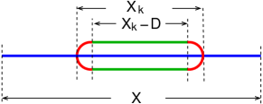
Figure 10: Illustration of the model used for theoretical prediction for a knot in a cone. The blue line represents an unknotted linear polymer of extension length $X$. The linear polymer overlaps with a ring polymer of extension $X_{\rm k}$. The diameter of the ring polymer hairpins (colored red) is approximately $D$, the diameter of the cone at the center of the the ring. The extension of the extended sections of the ring polymer (colored green) is thus $X_{\rm k}-D$.

We identify four main contributions to the free energy:

1. The free energy of the two hairpins, $F_{1}$.

2. The overlap free energy of the three subchains that lie between the two hairpins along the channel, $F_{2}$.

3. The confinement free energy of the two extended sections of the ring polymer (colored green in the figure), $F_{3}$.

4. The confinement free energy of the linear polymer (colored blue in the figure), $F_{4}$.

For the hairpin free energy, we use the results of a study by Chen.Chen (2017) In that study, a numerical solution to the Green’s function equations for an ideal chain confined to a channel yielded a hairpin free energy that could be approximated with the following equation:

$$F_{\rm hp}=\frac{2E_{m}}{\tilde{D}}-\frac{3}{2}\ln\left[\frac{A_{2}\tilde{D}+A_{0}\tilde{D}^{2}}{1+A_{1}\tilde{D}+A_{0}\tilde{D}^{2}}\right]+\ln 4,$$ (18)

where $\tilde{D}\equiv D/P$ and where the dimensionless numerical factors are $E_{m}=1.43557$, $A_{0}=1.0410$, $A_{1}=-0.6046$ and $A_{2}=1.2150$. For simplicity, we neglect the small variation of the $D$ over the span of the knot, which is located at position $Z_{\rm k}$. (Note that this approximation is valid only for very small cone angles. Carrying out calculations with and without it produced results with negligible difference for the cone angles used here.) Thus, the hairpin free energy is:

$$F_{1}(Z_{\rm k})=2F_{\rm hp}(D(Z_{\rm k})),$$ (19)

where the factor of 2 accounts for fact that there are two hairpins, and where

$$D(Z_{\rm k})=D_{0}+2Z_{\rm k}\tan\alpha.$$ (20)

As noted in Sec. IV.1, the overlap free energy for an S-loop or knot for a polymer confined to a cylinder in the Odijk regime is approximately

$$F_{\rm ov}=CD^{-5/3}P^{1/3}(X_{\rm k}-D),$$

where $X_{\rm k}-D$ is the span of the three overlapping polymer strands in the knot excluding the hairpins, and where the constant is estimated to be $C$=9.45. Thus,

$$F_{2}(Z_{\rm k},X_{\rm k})=C(D(Z_{\rm k}))^{-5/3}P^{-1/3}(X_{\rm k}-D(Z_{\rm k})).~{}~{}~{}~{}$$ (21)

For the contribution from the confinement free energy of the two extended portions of the ring, we neglect the small variation of the cone diameter along the span of the knot. The overlap free energy is thus

$$F_{3}(Z_{\rm k},X_{\rm k})=2a(X_{\rm k}-D(Z_{\rm k}))\left(D(Z_{\rm k})\right)^{-2/3}P^{-1/3},~{}~{}~{}~{}$$ (22)

where $a$=2.3565.Dai et al. (2016) In addition, the factor of 2 is due to the presence of two extended strands of the ring polymer, and $D(Z_{\rm k})$ is given by Eq. (20).

Finally, consider the free energy of the linear polymer in the cone. Since the contour length of the knotted polymer $L$ is the sum of the contour length for the linear polymer, $L^{\prime}$, and that of the ring polymer, it follows that:

$$L^{\prime}=L-\pi D(Z_{\rm k})-2(X_{\rm k}-D(Z_{\rm k})).$$

Thus,

$$L-(\pi-2)D(Z_{\rm k})-2X_{\rm k}=f(X),$$ (23)

where $f(X)$ is given by Eq. (14). It follows that:

$$X(Z_{\rm k},X_{\rm k})=f^{-1}(L-(\pi-2)D(Z_{\rm k})-2X_{\rm k}).$$ (24)

Using Eq. (17), the confinement free energy of the linear polymer in the cone is thus:

$$F_{4}(Z_{\rm k},X_{\rm k}) = \left(\frac{3a}{2b^{1/2}\tan\alpha}\right)\left[\tanh^{-1}\left(b^{1/2}\left(\frac{D(X)}{P}\right)^{1/3}\right)\right.$$ (25)

$$\left.-\tanh^{-1}\left(b^{1/2}\left(\frac{D_{0}}{P}\right)^{1/3}\right)\right],$$

where the dependence of $F_{4}$ on $Z_{\rm k}$ and $X_{\rm k}$ arises from the relation for the extension length $X$ in Eq. (24).

The total free energy if the knotted polymer is given by the sum

$$F(Z_{\rm k})=F_{1}(Z_{\rm k})+F_{2}(Z_{\rm k},X_{\rm k})+F_{3}(Z_{\rm k},X_{\rm k})+F_{4}(Z_{\rm k},X_{\rm k}),$$

where the free energy contributions are given by Eqs. (19), (21), (22) and (25). Finally, the dependence of $F$ on the knot span $X_{\rm k}$ must be removed. Note that $X_{\rm k}$ is a fluctuating variable whose mean and variance depends on $Z_{\rm k}$, the position of the knot along the channel. To estimate the variation of $X_{\rm k}$ with $Z_{\rm k}$, we have chosen the following procedure. A set of simulations for a knotted polymer in a cylindrical channel were carried out to measure $F(X)$ and $X_{\rm k}(X)$ for various values of channel diameter $D$. At each $D$, the mean value of $X_{\rm k}$ was calculated

$$\bar{X}_{\rm k}(D)=\frac{\int X_{\rm k}(X;D)e^{-\beta F(X;D)}dX}{\int e^{-\beta F(X;D)}dX},$$ (27)

where the integrals were approximated using discrete summations. Applying this result to the conical channel requires the $Z_{\rm k}$-dependence of $D$, which is provided by Eq. (20). Figure 11 shows a comparison of each of the contributions for a $3_{1}$ knot for a system with $N$=200, $\kappa=15$, $D_{0}$=4.0, and $\alpha$=$0.57^{\circ}$. The hairpin contribution to free energy is the dominant term, a consequence of the narrowness of the conical channel.

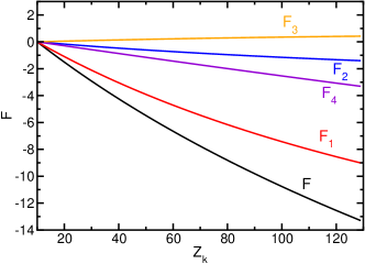
Figure 11: Variation of each contribution to the predicted free energy with knot position. The contributions $F_{1}$, $F_{2}$, $F_{3}$ and $F_{4}$ are calculated using Eqs. (19), (21), (22), and (25), respectively, and $F$ is the sum of the contributions. The predictions are calculated for a $3_{1}$ knot, $N$=200, $\kappa=15$, $D_{0}$=4.0, and $\alpha$=$0.57^{\circ}$.

References

- Dai et al. (2016) L. Dai, C. B. Renner, and P. S. Doyle, Adv. Colloid Interface Sci. 232, 80 (2016).
- Reisner et al. (2012) W. Reisner, J. N. Pedersen, and R. H. Austin, Rep. Prog. Phys. 75, 106601 (2012).
- Dorfman et al. (2012) K. D. Dorfman, S. B. King, D. W. Olson, J. D. Thomas, and D. R. Tree, Chem. Rev. 113, 2584 (2012).
- Reisner et al. (2010) W. Reisner, N. B. Larsen, A. Silahtaroglu, A. Kristensen, N. Tommerup, J. O. Tegenfeldt, and H. Flyvbjerg, Proc. Natl. Acad. Sci. U.S.A. 107, 13294 (2010).
- Marie et al. (2013) R. Marie, J. N. Pedersen, D. L. Bauer, K. H. Rasmussen, M. Yusuf, E. Volpi, H. Flyvbjerg, A. Kristensen, and K. U. Mir, Proc. Natl. Acad. Sci. U.S.A. 110, 4893 (2013).
- Lam et al. (2012) E. T. Lam, A. Hastie, C. Lin, D. Ehrlich, S. K. Das, M. D. Austin, P. Deshpande, H. Cao, N. Nagarajan, M. Xiao, and P.-Y. Kwok, Nature Biotech. 30, 771 (2012).
- Hastie et al. (2013) A. R. Hastie, L. Dong, A. Smith, J. Finklestein, E. T. Lam, N. Huo, H. Cao, P.-Y. Kwok, K. R. Deal, and J. Dvorak, PloS one 8, e55864 (2013).
- Dorfman (2013) K. D. Dorfman, AIChE J. 59, 346 (2013).
- Müller and Westerlund (2017) V. Müller and F. Westerlund, Lab Chip 17, 579 (2017).
- Orlandini (2017) E. Orlandini, J. Phys. A 51, 053001 (2017).
- Arsuaga et al. (2005) J. Arsuaga, M. Vazquez, P. McGuirk, S. Trigueros, and J. Roca, Proc. Natl. Acad. Sci. U.S.A. 102, 9165 (2005).
- Rybenkov et al. (1993) V. V. Rybenkov, N. R. Cozzarelli, and A. V. Vologodskii, Proc. Natl. Acad. Sci. U.S.A. 90, 5307 (1993).
- Bao et al. (2003) X. R. Bao, H. J. Lee, and S. R. Quake, Phys. Rev. Lett. 91, 265506 (2003).
- Ercolini et al. (2007) E. Ercolini, F. Valle, J. Adamcik, G. Witz, R. Metzler, P. De Los Rios, J. Roca, and G. Dietler, Phys. Rev. Lett. 98, 058102 (2007).
- Tang et al. (2011) J. Tang, N. Du, and P. S. Doyle, Proc. Natl. Acad. Sci. U. S. A. 108, 16153 (2011).
- Renner and Doyle (2015) C. B. Renner and P. S. Doyle, Soft Matter 11, 3105 (2015).
- Plesa et al. (2016) C. Plesa, D. Verschueren, S. Pud, J. van der Torre, J. W. Ruitenberg, M. J. Witteveen, M. P. Jonsson, A. Y. Grosberg, Y. Rabin, and C. Dekker, Nat. Nanotechnol. 11, 1093 (2016).
- Klotz et al. (2017) A. R. Klotz, V. Narsimhan, B. W. Soh, and P. S. Doyle, Macromolecules 50, 4074 (2017).
- Soh et al. (2018a) B. W. Soh, V. Narsimhan, A. R. Klotz, and P. S. Doyle, Soft Matter 14, 1689 (2018a).
- Amin et al. (2018) S. Amin, A. Khorshid, L. Zeng, P. Zimny, and W. Reisner, Nat. Commun. 9, 1506 (2018).
- Sharma et al. (2019) R. K. Sharma, I. Agrawal, L. Dai, P. S. Doyle, and S. Garaj, Nat. Commun. 10, 1 (2019).
- Klotz et al. (2018) A. R. Klotz, B. W. Soh, and P. S. Doyle, Phys. Rev. Lett. 120, 188003 (2018).
- Soh et al. (2018b) B. W. Soh, A. R. Klotz, and P. S. Doyle, Macromolecules 51, 9562 (2018b).
- Metzler et al. (2006) R. Metzler, W. Reisner, R. Riehn, R. Austin, J. Tegenfeldt, and I. M. Sokolov, Europhys. Lett. 76, 696 (2006).
- Reifenberger et al. (2015) J. G. Reifenberger, K. D. Dorfman, and H. Cao, Analyst 140, 4887 (2015).
- Ma and Dorfman (2020) Z. Ma and K. D. Dorfman, Macromolecules (2020).
- Micheletti and Orlandini (2014) C. Micheletti and E. Orlandini, ACS Macro Lett. 3, 876 (2014).
- Jain and Dorfman (2017) A. Jain and K. D. Dorfman, Biomicrofluidics 11, 024117 (2017).
- Micheletti et al. (2011) C. Micheletti, D. Marenduzzo, and E. Orlandini, Phys. Rep. 504, 1 (2011).
- Mobius et al. (2008) W. Mobius, E. Frey, and U. Gerland, Nano Lett. 8, 4518 (2008).
- Micheletti and Orlandini (2012) C. Micheletti and E. Orlandini, Soft Matter 8, 10959 (2012).
- Orlandini and Micheletti (2013) E. Orlandini and C. Micheletti, J. Biol. Phys. 39, 267 (2013).
- Nakajima and Sakaue (2013) C. H. Nakajima and T. Sakaue, Soft Matter 9, 3140 (2013).
- Suma et al. (2015) A. Suma, E. Orlandini, and C. Micheletti, J. Phys.: Condens. Matter 27, 354102 (2015).
- Dai et al. (2015a) L. Dai, C. B. Renner, and P. S. Doyle, Macromolecules 48, 2812 (2015a).
- Dai et al. (2015b) L. Dai, C. B. Renner, and P. S. Doyle, Phys. Rev. Lett. 114, 037801 (2015b).
- Grosberg and Rabin (2007) A. Y. Grosberg and Y. Rabin, Phys. Rev. Lett. 99, 217801 (2007).
- Dai et al. (2014) L. Dai, C. B. Renner, and P. S. Doyle, Macromolecules 47, 6135 (2014).
- Polson et al. (2017) J. M. Polson, A. F. Tremblett, and Z. R. N. McLure, Macromolecules 50, 9515 (2017).
- Polson (2018) J. M. Polson, Macromolecules 51, 5962 (2018).
- Bell et al. (2017) N. A. Bell, K. Chen, S. Ghosal, M. Ricci, and U. F. Keyser, Nat. Commun. 8, 1 (2017).
- Nikoofard et al. (2013) N. Nikoofard, H. Khalilian, and H. Fazli, J. Chem. Phys. 139, 074901 (2013).
- Nikoofard and Fazli (2015) N. Nikoofard and H. Fazli, Soft Matter 11, 4879 (2015).
- Kumar and Kumar (2018) S. Kumar and S. Kumar, Physica A 499, 216 (2018).
- Polson and Heckbert (2019) J. M. Polson and D. R. Heckbert, Phys. Rev. E 100, 012504 (2019).
- Frenkel and Smit (2002) D. Frenkel and B. Smit, Understanding Molecular Simulation: From Algorithms to Applications, 2nd ed. (Academic Press, London, 2002) Chap. 7.
- Polson et al. (2013) J. M. Polson, M. F. Hassanabad, and A. McCaffrey, J. Chem. Phys. 138, 024906 (2013).
- Tubiana et al. (2011) L. Tubiana, E. Orlandini, and C. Micheletti, Prog. Theor. Phys. Supp. 191, 192 (2011).
- Odijk (2008) T. Odijk, Phys. Rev. E 77, 060901(R) (2008).
- Caraglio et al. (2015) M. Caraglio, C. Micheletti, and E. Orlandini, Phys. Rev. Lett. 115, 188301 (2015).
- Odijk (2006) T. Odijk, J. Chem. Phys. 125, 204904 (2006).
- Chen (2017) J. Z. Y. Chen, Phys. Rev. Lett. 118, 247802 (2017).
- Matthews et al. (2012) R. Matthews, A. A. Louis, and C. N. Likos, ACS Macro Lett. 1, 1352 (2012).
- Poier et al. (2014) P. Poier, C. N. Likos, and R. Matthews, Macromolecules 47, 3394 (2014).