Pair production due to an electric field in 1+1 dimensions and the validity of the semiclassical approximation

Abstract

Solutions to the backreaction equation in 1+1-dimensional semiclassical electrodynamics are obtained and analyzed when considering a time-varying homogeneous electric field initially generated by a classical electric current, coupled to either a quantized scalar field or a quantized spin-$\frac{1}{2}$ field. Particle production by way of the Schwinger effect leads to backreaction effects that modulate the electric field strength. Details of the particle production process are investigated along with the transfer of energy between the electric field and the particles. The validity of the semiclassical approximation is also investigated using a criterion previously implemented for chaotic inflation and, in an earlier form, semiclassical gravity. The criterion states that the semiclassical approximation will break down if any linearized gauge-invariant quantity constructed from solutions to the linear response equation, with finite nonsingular data, grows rapidly for some period of time. Approximations to homogeneous solutions of the linear response equation are computed and it is found that the criterion is violated when the maximum value, $E_{\rm max}$, obtained by the electric field is of the order of the critical scale for the Schwinger effect, $E_{\rm max}\sim E_{\rm crit}\equiv m^{2}/q$, where $m$ is the mass of the quantized field and $q$ is its electric charge. For these approximate solutions the criterion appears to be satisfied in the extreme limits $\frac{qE_{\rm max}}{m^{2}}\ll 1$ and $\frac{qE_{\rm max}}{m^{2}}\gg 1$.

I Introduction

The semiclassical approximation has been commonly used among a wide variety of physical scenarios where a quantized field on a classical background is investigated, with interesting phenomena emerging from such considerations including the decay of an electric field by the Schwinger effect schwinger , particle creation in an expanding universe parker66 , and black hole evaporation via the Hawking effect hawking (see also Refs. parker-toms ; birrell-davies and references therein). Consider for instance quantum electrodynamics, described in terms of an electromagnetic potential $A_{\mu}$ and a Dirac field $\psi$, with classical action $S[A_{\mu},\bar{\psi},\psi]$. The semiclassical theory can be formally described using the concept of the effective action $\Gamma[A_{\mu}]$, obtained by functional integration of the matter degrees of freedom qftbook

$$\exp{i\Gamma[A_{\mu}]}=\int D\bar{\psi}D\psi\exp{iS[A_{\mu},\bar{\psi},\psi]}\quad.$$ (1)

Within this framework the (semiclassical) Maxwell field equations take the form

$$\partial_{\mu}F^{\mu\nu}=q\langle 0_{A}|\bar{\psi}\gamma^{\mu}\psi|0_{A}\rangle\quad,$$ (2)

and replace the proper Maxwell equations of the full quantized theory in the Schwinger-Dyson form $\partial_{\mu}\langle F^{\mu\nu}\rangle=q\langle\bar{\psi}\gamma^{\mu}\psi\rangle$. In Eqs. (1) and (2) the electromagnetic field is treated as a purely classical entity. Moreover, the right-hand side of Eq. (2) is implicitly a function of $A_{\mu}$ in the sense that the assumed vacuum depends on $A_{\mu}$. This is so because the modes of the charged Dirac field, defining the appropriate vacuum $|0_{A}\rangle$, satisfy equations involving the background field $A_{\mu}$. This semiclassical approach is usually regarded as a truncated and effective version of the fully quantized theory, with a limited range of validity.

One advantage of the semiclassical viewpoint is that it provides a clear description of the spontaneous particle creation phenomena. The nonzero imaginary part of the effective action $\Gamma[A_{\mu}]$ indicates the quantum instability of the vacuum $|0_{A}\rangle$ and the corresponding pair creation process schwinger . This phenomena can be better understood in the canonical language: a positive-frequency solution of the Dirac equation $(i\not{D}-m)\psi=0$ at early times will evolve into a superposition of positive- and negative-frequency solutions at late times (this was first described for a gravitational background parker66 ). The semiclassical approach encapsulates in a clear way this very important effect. The original calculation by Schwinger schwinger involved a background field calculation in which the electric field $E$ is constant in both space and time. A particle production rate was obtained. The dependence on the coupling constant $q$ displayed an essential singularity $e^{-m^{2}/qE}$, showing the nonperturbative nature of the Schwinger effect. The damping of the electric field can be deduced from this particle production rate. The real part of the (Heisenberg-Euler) effective action can also account for perturbative effects, such as light-by-light scattering, in agreement with the exact one-loop calculation in the limit of low-frequency light, or the running of the effective coupling constant.

Subsequently the semiclassical backreaction equation was solved for an electromagnetic field coupled to a massive scalar field or a massive spin-$\frac{1}{2}$ field in 1+1 dimensions (D) Kluger91 ; Kluger92 ; Kluger93 and 3+1D Kluger93 ; Tanji ; stat-FT . The electric field was assumed to be homogeneous in space, but was allowed to vary in time in response to the electric current that occurs when the produced particles are accelerated by the electric field. It was found the counter-electric field produced by this current initially starts to negate the original background electric field. Eventually the background field is completely canceled, but by this time there is a significant electric current due to particle production and the result is that the particles keep moving which generates an electric field in the opposite direction. The process continues and the particles end up undergoing plasma oscillations with an overall electric field oscillation in time. Similar studies have also been done by solving the Vlasov equation with a source term to account for particle production Kluger91 ; Kluger92 ; Kluger93 ; Bloch , using lattice simulations lattice-1 ; lattice-2 , and classical statistical field theory techniques stat-FT .

In this paper we obtain and further study solutions to the semiclassical backreaction equation in 1+1D for both scalar and spin-$\frac{1}{2}$ fields coupled to an electromagnetic field initially generated by a homogeneous, classical current. We have two primary goals. The first is to study the details of the particle production process when backreaction effects have been taken into account, including also the transfer of energy between the electric field and the created particles. The second goal is to estimate the importance of certain types of quantum fluctuations and use the results to assess the validity of the semiclassical approximation.

We study three classical current profiles which generate an electric field that is initially zero. The first is similar to the previous cases in that the current is proportional to a delta function potential and the electric field goes from zero to a constant value instantaneously. A second profile involves a sudden turn on of the classical current but a gradual turn on of the electric field. The third profile is that of the Sauter pulse Sauter in which the current is in the form of a smooth pulse that has a significant value only for a finite period of time. For the Sauter pulse the turn on and, if quantum effects are ignored, the turn off of both the current and the electric field are very gradual. In all three cases there is a well-defined vacuum state for the quantum fields since the electric field is initially zero. The semiclassical backreaction equation is solved numerically both in the case of semiclassical scalar and spinor electrodynamics. To our knowledge the semiclassical backreaction equations have not been generically studied for the second and third classical current profiles. The first one has been considered in Refs. Tanji ; stat-FT ; lattice-1 ; lattice-2 ; Bloch .

The particle production process for individual modes of the quantum field has previously been studied in background field calculations where the electric field is either constant and-mot-I ; dunne-part-prod or is gradually turned on and then off and-mot-san . It was found that a single particle creation event occurs for many modes when the electric field is either constant or approximately constant. Here, we consider particle production when backreaction effects are taken into account. Because of the plasma oscillations, there is a richer evolution for some modes that involves multiple particle creation events and can also involve particle destruction events. We do this for individual modes for the delta function classical current profile.

For completeness, and to give better insight into the particle creation process, we also compute the total number of particles produced for all three profiles and the energy density of the produced particles for the delta function current profile. The energy density of the particles is compared with the energy density of the electric field. Similar calculations have been done previously in $1+1$D using lattice simulations  lattice-1 and in $3+1$D using canonical quantization Tanji and classical statistical field theory techniques stat-FT .

We compute the energy density of the quantum field using the continuous adiabatic regularization prescription, obtaining compatible results. The agreement between both approaches for Dirac massless fermions can be easily understood since the full QED₂ model is integrable Schwingermass and particle production can be well described within the semiclassical framework. The presence of a nonzero mass breaks integrability and hence one could expect it to also break the accuracy of the semiclassical picture.

The validity of the semiclassical approximation is studied here by estimating the importance of some of the quantum fluctuations. The semiclassical approximation breaks down if quantum fluctuations are too large. We use a criterion for the validity of the semiclassical approximation that has been previously applied to the process of preheating in models of chaotic inflation validitypreheating . An earlier version of the criterion has also been used to study the validity of the semiclassical approximation for free scalar fields in flat space when the fields are in the Minkowski vacuum state validitygravity and for the conformally invariant scalar field in the Bunch-Davies state in de Sitter space in the usual spatially flat cosmological coordinates validitydeSitter . To our knowledge no similar study of the validity of the semiclassical approximation has been done previously for scalar electrodynamics or quantum electrodynamics when particle creation occurs due to the presence of a strong electric field.

The method we use to study the validity of the semiclassical approximation involves an analysis of solutions to the linear response equation which can be obtained by perturbing the semiclassical backreaction equation. In general, the linear response equation obtained in this way is an integro-differential equation which involves an integral over the retarded two-point correlation function for the source term in the semiclassical backreaction equation. In this case, that is the two-point correlation function for the electric current. While the general form is known, the specific forms for the case of a homogeneous electric field in 1+1D coupled to either a massive scalar field or a spin-$\frac{1}{2}$ field has not previously been derived. We do so in the Appendix for both of these cases.

Although the linear response equation can be solved directly, there is a simpler method which can be used to obtain an approximate solution which should be valid at early times if the exact solution is relatively small. The method involves computing the difference $\Delta E$ between two solutions to the semiclassical backreaction equation which have similar starting values at a given time. This method was used to investigate the validity of the semiclassical approximation during the preheating phase of chaotic inflation in Ref. validitypreheating . It works for the homogeneous solutions to the linear response equation that we consider here.

The paper is organized as follows. In Sec. II brief reviews are given of the quantization of complex charged scalar and spin-$\frac{1}{2}$ fields in electrodynamics. The semiclassical backreaction equations are also discussed along with the renormalization techniques used. In Sec. III the details of the particle production process are investigated for the case of a classical current profile proportional to a delta function. Also discussed is the transfer of energy between the electric field and the created particles. The criterion for the validity of the semiclassical approximation that we use is discussed in Sec. IV where both the general form and the specific form of the linear response equation are displayed for the separate cases of a scalar field and spin-$\frac{1}{2}$ field coupled to the electromagnetic field. In Sec. V some of the results of numerical calculations we have made related to the validity of the semiclassical approximation are presented and discussed. A summary of our results and some conclusions are given in Sec. VI. The Appendix contains derivations of the specific contributions to the linear response equations from the current-current commutators when scalar fields and spin $\frac{1}{2}$ fields are coupled to the electromagnetic field.

II Quantization and renormalization of complex scalar and
spin-$\frac{1}{2}$ fields

In this section we will briefly describe the models under consideration: a quantized complex scalar field and a quantized Dirac field, both interacting with a background electromagnetic field generated by a prescribed classical source. For the two systems under investigation, we restrict our analysis to a $1+1$D Minkowski space and assume that the background electric field is spatially homogeneous so that $E=E(t)$ in a given reference frame. We use units such that $\hbar=c=1$ and our convention for the metric signature is $(-,+)$.

II.1 Scalar field

The classical action representing a scalar field $\phi(t,x)$ coupled to a background electromagnetic field is

$$S=\int d^{2}x\bigg{[}-\frac{1}{4}F_{\mu\nu}F^{\mu\nu}+A_{\mu}J_{C}^{\mu}-D_{\mu}\phi^{\dagger}D^{\mu}\phi-m^{2}\phi^{\dagger}\phi\bigg{]}\quad,$$ (3)

where $F_{\mu\nu}=\partial_{\mu}A_{\nu}-\partial_{\nu}A_{\mu}$ is the electromagnetic field-strength tensor, the mass of scalar field excitations is given by $m$, and $D_{\mu}=\partial_{\mu}-iqA_{\mu}$ is the gauge-covariant derivative required to make the action gauge invariant. $J_{C}^{\mu}$ is a classical and conserved external source. Variation of Eq. (3) with respect to the vector potential yields the classical Maxwell equations

$$-\Box A^{\mu}+\partial^{\mu}\partial_{\nu}A^{\nu}=J^{\mu}_{C}+J^{\mu}_{Q}\quad,$$ (4)

where the source term $J^{\mu}_{Q}$ induced by the scalar field is given by

$$J^{\mu}_{Q}=\eta^{\mu\nu}\bigg{[}-iq\bigg{(}\phi^{\dagger}\partial_{\nu}\phi-\left(\partial_{\nu}\phi^{\dagger}\right)\phi\bigg{)}-2q^{2}A_{\nu}\left(\phi^{\dagger}\phi\right)\bigg{]}\quad.$$ (5)

The field equation for $\phi(t,x)$ is $\left(D^{\mu}D_{\mu}-m^{2}\right)\phi(t,x)=0$. We choose the Lorentz gauge $\partial_{\mu}A^{\mu}=0$, and fix the vector potential in the convenient form

$$A^{\mu}=(0,A(t))\;,$$ (6)

which therefore yields $F_{01}=\partial_{0}A_{1}=\dot{A}=-E$. The field equation reduces to

$$\bigg{[}-\partial_{t}^{2}+\partial_{x}^{2}-2iqA(t)\partial_{x}-q^{2}A^{2}(t)-m^{2}\bigg{]}\phi(t,x)=0\quad.$$ (7)

Quantizing the scalar field and expanding it in terms of modes yields

$$\phi(t,x)=\frac{1}{\sqrt{2\pi}}\int_{-\infty}^{\infty}dk\bigg{[}a_{k}U_{k}(t,x)+b_{k}^{\dagger}V_{k}(t,x)\bigg{]}\ .$$ (8)

where $a_{k},a_{k}^{\dagger},b_{k},\textnormal{and}\,b^{\dagger}_{k}$ are the usual creation and annihilation operators obeying the commutation relations $[a_{k},a_{k^{{}^{\prime}}}^{\dagger}]=[b_{k},b_{k^{{}^{\prime}}}^{\dagger}]=\delta(k-k^{{}^{\prime}})$. Due to spatial homogeneity we can write the modes $U_{k}(t,x)$ and $V_{k}(t,x)$ in the convenient form $U_{k}(t,x)=f_{k}(t)e^{ikx}$, $V_{k}(t,x)=f_{-k}^{*}(t)e^{-ikx}$, where $f_{k}(t)$ satisfies the ordinary differential equation

$$\ddot{f}_{k}(t)+\bigg{[}\left(k-qA\right)^{2}+m^{2}\bigg{]}f_{k}(t)=0$$ (9)

and is normalized using the Wronskian condition

$$f_{k}\dot{f}_{k}^{*}-f_{k}^{*}\dot{f}_{k}=i.$$ (10)

This allows us to recast the scalar field mode decomposition as

$$\phi(t,x)=\frac{1}{\sqrt{2\pi}}\int dk\bigg{[}a_{k}f_{k}(t)+b_{-k}^{\dagger}f_{k}^{*}(t)\bigg{]}e^{ikx}\;.$$ (11)

II.2 Spin-$\frac{1}{2}$ field

The classical action representing a spin-$\frac{1}{2}$ field $\psi(t,x)$ coupled to a background electric field is

$$S=\int d^{2}x\,\bigg{[}-\frac{1}{4}F_{\mu\nu}F^{\mu\nu}+A_{\mu}J_{C}^{\mu}+i\bar{\psi}\gamma^{\mu}D_{\mu}\psi-m\bar{\psi}\psi\bigg{]}\quad.$$ (12)

where $\bar{\psi}=\psi^{\dagger}\gamma^{0}$, with $F^{\mu\nu}$ and $D_{\mu}$ defined the same as for the scalar field case. The Dirac matrices $\gamma^{\mu}$ satisfy the anticommutation relations $\{\gamma^{\mu},\gamma^{\nu}\}=-2\eta^{\mu\nu}$. As for the scalar field, $J_{C}$ is an external classical source. The Maxwell equations include the source term induced by the field $\psi$

$$J^{\mu}_{Q}=q\,\bar{\psi}\,\gamma^{\mu}\,\psi\quad.$$ (13)

The field equation for $\psi(t,x)$ is the Dirac equation $\big{(}i\,\gamma^{\mu}D_{\mu}-m\,\big{)}\psi(t,x)=0$. With the gauge choice (6) the explicit form of the Dirac equation is

$$\bigg{[}i\,\gamma^{t}\partial_{t}+i\,\gamma^{x}\partial_{x}+q\,\gamma^{x}A(t)-m\bigg{]}\psi(t,x)=0\quad.$$ (14)

Quantizing the spin-$\frac{1}{2}$ field and expanding it in terms of modes yields

$$\psi(t,x) = \int_{-\infty}^{\infty}dk\,\bigg{[}B_{k}u_{k}(t,x)+D_{k}^{\dagger}v_{k}(t,x)\bigg{]}\;,$$ (15)

where here $B_{k},B_{k}^{\dagger},D_{k},\,\textnormal{and}\,D_{k}^{\dagger}$ are the usual creation and annihilation operators obeying the anticommutation relations $\{B_{k},B^{\dagger}_{k^{{}^{\prime}}}\}=\{D_{k},D^{\dagger}_{k^{{}^{\prime}}}\}=\delta(k-k^{{}^{\prime}})$. Using the formalism introduced in Refs. FN ; BNP , we can construct two independent spinor solutions as follows

$$u_{k}(t,x)=\frac{e^{ikx}}{\sqrt{2\pi}}{\small\left({\begin{array}[]{c}h_{k}^{I}(t)\\ -h_{k}^{II}(t)\end{array}}\right)}\quad,\quad v_{k}(t,x)=\frac{e^{-ikx}}{\sqrt{2\pi}}{\small\left({\begin{array}[]{c}h_{-k}^{II*}(t)\\ h_{-k}^{I*}(t)\end{array}}\right)}.$$ (16)

Utilizing the Weyl representation of the Dirac matrices $\gamma^{\mu}$

$$\gamma^{t}=\left({\begin{array}[]{cc}0&1\\ 1&0\\ \end{array}}\right)\quad,\quad\gamma^{x}=\left({\begin{array}[]{cc}0&1\\ -1&0\\ \end{array}}\right)\quad,\quad\gamma^{5}=\gamma^{t}\gamma^{x}=\left({\begin{array}[]{cc}-1&0\\ 0&1\\ \end{array}}\right)\ ,$$ (17)

one can show that $h_{k}^{I}(t)$ and $h_{k}^{II}(t)$ are solutions of the mode equations

$$\dot{h}_{k}^{I}-i\left(k-qA\right)h_{k}^{I}-i\,m\,h_{k}^{II} = 0\,,$$ (18a)

$$\dot{h}_{k}^{II}+i\left(k-qA\right)h_{k}^{II}-i\,m\,h_{k}^{I} = 0.$$ (18b)

The normalization condition $|h_{k}^{I}|^{2}+|h_{k}^{II}|^{2}=1$ ensures that the standard anticommutation relations between the creation and annihilation operators are satisfied.

II.3 Semiclassical backreaction equation and renormalization

A simple way to obtain the semiclassical backreaction equation is to replace $J^{\mu}_{Q}$ in Eq. (4) with $\langle J^{\mu}_{Q}\rangle$ and then use Eq. (6) and either (11) or Eq. (15), with the result

$$\frac{d^{2}}{dt^{2}}A(t)=-\frac{d}{dt}E(t)=J_{C}+\langle J_{Q}\rangle\quad.$$ (19)

Here we have simplified the notation by omitting the superscript $x$ on $J_{C}$ and $J_{Q}$ since in this case the $t$ component of these vectors vanishes. When particle production occurs the background electric field accelerates the produced particles creating a current which then reacts back on this electric field. In the semiclassical approximation this current is $\langle J_{Q}\rangle$. The net electric field $E(t)$ is then generated by both the classical current $J_{C}$ and the current from the created particles $\langle J_{Q}\rangle$.

We now obtain the generic forms of the finite, physical expression of $\langle J_{Q}\rangle$ for both scalar and fermion fields. This is nontrivial since the formal expressions for the current are quadratic in the quantized fields. Here we will explain how the ultraviolet divergences can be tamed by using the so-called adiabatic regularization method. The method was originally proposed to obtain finite expectation values for the stress-energy tensors of scalar fields in expanding universes parker-fulling ; Birrell78 ; Anderson-Parker (see also Refs. parker-toms ; birrell-davies for scalar fields and Refs. rio1 ; rio2 ; rio3 ; ghosh1 ; ghosh2 ; BFNV for fermion fields). The adiabatic method has been adapted to treat spatially homogeneous electric backgrounds in Refs. Cooper-Mottola89 ; CMRA ; Kluger92 , and it has been improved to make it consistent with gravity in Refs. FN ; FNP ; FNP2 and connected to the DeWitt-Schwinger proper-time expansion in Ref. BNP20 . Here we follow the procedure proposed in Ref. FN ; FNP ; FNP2 .

II.3.1 Scalar field

It is useful to symmetrize the current operator for the scalar field with the result

$$J^{\mu}_{Q}=\frac{1}{2}\eta^{\mu\nu}\bigg{[}-iq\bigg{(}\phi^{\dagger}\partial_{\nu}\phi-\left(\partial_{\nu}\phi^{\dagger}\right)\phi\bigg{)}+iq\bigg{(}\phi\partial_{\nu}\phi^{\dagger}-\left(\partial_{\nu}\phi\right)\phi^{\dagger}\bigg{)}-2q^{2}A_{\nu}\bigg{(}\phi^{\dagger}\phi+\phi\phi^{\dagger}\bigg{)}\bigg{]}\quad.$$ (20)

Using Eq. (6) and evaluating Eq. (20) in the vacuum state gives for the nontrivial spatial component

$$\langle J_{Q}\rangle=\frac{q}{\pi}\int_{-\infty}^{\infty}dk\,\bigg{(}k-qA(t)\bigg{)}|f_{k}(t)|^{2}\quad.$$ (21)

Note that the $\mu=0$ component of the current is identically zero, meaning that no net charge is created. The integral (21) contains ultraviolet divergences and hence must be renormalized. Since the external electric field is assumed to be spatially homogeneous, it is especially convenient to use an extension of the adiabatic regularization method. For scalar fields the procedure is based on the standard WKB-type expansion of the field modes. In our case one writes the ansatz

$$f_{k}(t)=\frac{1}{\sqrt{2\Omega_{k}(t)}}e^{-i\int^{t}\Omega_{k}(t^{\prime})dt^{\prime}}\quad,$$ (22)

where $\Omega_{k}$ is expanded in powers of derivatives of $A(t)$, as $\Omega_{k}=\omega^{(0)}+\omega^{(1)}+\omega^{(2)}+\cdots$. The leading term $\omega^{(0)}$ is assumed to be of zeroth adiabatic order, while $\omega^{(1)}$ is of adiabatic order one, etc. The choice of the leading-order term $\omega^{(0)}$ determines univocally the subsequent orders. A natural possibility Cooper-Mottola89 is $\omega^{(0)}=\sqrt{(k-qA)^{2}+m^{2}}$, which assumes that $A(t)$ should be considered as a variable of adiabatic order zero, $\dot{A}$ of adiabatic order one, etc.

However, $A(t)$ is intrinsically a dimensionful quantity and this suggests an alternative possibility. As proposed in Refs. FN ; FNP , one can also choose $\omega^{(0)}\equiv\omega=\sqrt{k^{2}+m^{2}}$. This choice is attached to the adiabatic assignment of one for $A(t)$, while $\dot{A}$ is considered to be of adiabatic order two, etc. This second possibility is actually the only consistent possibility in the presence of both electromagnetic and gravitational backgrounds. We then obtain

$$\langle J_{Q}\rangle_{\textnormal{ren}}=\frac{q}{\pi}\int_{-\infty}^{\infty}dk\,\bigg{[}\bigg{(}k-qA(t)\bigg{)}|f_{k}(t)|^{2}-\frac{k}{2\omega}+\frac{q\,m^{2}}{2\omega^{3}}A(t)\bigg{]}\quad.$$ (23)

Similarly, one can also determine the renormalized energy density $\langle T_{00}\rangle=\langle\rho\rangle$ induced by the quantized field

$$\langle\rho\rangle_{\rm ren}=\frac{1}{2\pi}\int_{-\infty}^{\infty}dk\left[|\dot{f}_{k}(t)|^{2}+\bigg{(}m^{2}+\big{(}k-qA(t)\big{)}^{2}\bigg{)}|f_{k}(t)|^{2}-\omega+\frac{kq}{\omega}A(t)-\frac{m^{2}q^{2}}{2\omega^{3}}A^{2}(t)\right]\quad.$$

II.3.2 Spin-$\frac{1}{2}$ field

For the spin-$\frac{1}{2}$ field the appropriate antisymmetrized term is parker-toms

$$J^{\mu}_{Q}=\frac{q}{2}[\bar{\psi},\gamma^{\mu}\psi].$$ (25)

The expression for $\mu=0$ corresponds to the induced electric charge and, as expected, $\langle J^{0}_{Q}\rangle$ is identically zero, i.e. no net charge is created. The renormalized expression for the spatial component of the spin-$\frac{1}{2}$ current evaluated in the vacuum state is FN ; FNP2

$$\langle J_{Q}\rangle_{\textnormal{ren}}=\frac{q}{2\pi}\int_{-\infty}^{\infty}dk\,\bigg{[}|h_{k}^{I}(t)|^{2}-|h_{k}^{II}(t)|^{2}+\frac{k}{\omega}-\frac{q\,m^{2}}{\omega^{3}}A(t)\bigg{]}\quad.$$ (26)

It is particularly interesting to consider the massless case where the first two terms in the above integral cancel and the expression for the current becomes

$$\langle J_{Q}\rangle_{\textnormal{ren}}=-\frac{q^{2}}{\pi}A(t)\quad.$$ (27)

This result is consistent with the two-dimensional axial anomaly

$$\partial_{\mu}\langle J^{\mu}_{5}\rangle_{\textnormal{ren}}=\frac{q}{\pi}\epsilon^{\mu\nu}F_{\mu\nu}\quad,$$ (28)

where $J^{\mu}_{5}=\bar{\psi}\gamma^{\mu}\gamma^{5}\psi$ and $J^{\mu}_{Q}=-q\epsilon^{\mu\nu}J_{\nu 5}$. Furthermore, the renormalized energy density is given by

$$\langle\rho\rangle_{\rm ren}=\frac{1}{2\pi}\int_{-\infty}^{\infty}dk\bigg{[}i\left[h_{k}^{II}(t)\dot{h}_{k}^{II*}(t)+h_{k}^{I}(t)\dot{h}_{k}^{I*}(t)\right]+\omega-\frac{kq}{\omega}A(t)+\frac{m^{2}q^{2}}{2\omega^{3}}A^{2}(t)\bigg{]}\quad.$$ (29)

III Particle production and energy conservation in the semiclassical framework

In this section we study both the details of the particle production process and the transfer of energy between the electric field and the produced particles for some solutions to the semiclassical backreaction equation for the delta function current profile mentioned in the Introduction.

The vacuum instability due to pair production was first realized by Heisenberg and Euler Heisenberg1936 , who predicted, on the basis of an effective action for a constant and homogeneous electromagnetic background, a pair production rate in an electric field of order $\sim q^{2}E^{2}e^{-\frac{m^{2}\pi}{qE}}$. Schwinger, using the modern language of QED, computed the imaginary part of the one-loop effective action, also for a homogeneous and constant electric field, to evaluate the vacuum persistence amplitude (for a historical perspective, see Ref. dunne ). From the exponential factor one notes immediately that the order of the critical scale for pair production can be defined to be

$$E_{\rm crit}\sim m^{2}/q\;.$$ (30)

For some of the numerical work described in the following sections we compare the classical electric field to $E_{\rm crit}$ and for those comparisons we take $E_{\rm crit}$ to be equal to $m^{2}/q$, as is customary in the literature on the Schwinger effect.

While particle production in quantum field theory is a nonlocal process, for free quantum fields such as the ones we are considering, it is possible to define a time-dependent particle number that is based on the WKB approximation for the modes of the quantum field. This has been done previously in the electric field case in Refs. and-mot-I ; dunne-part-prod ; and-mot-san where background electric fields were considered. While there was some variation in the details depending on the order of the WKB approximation used, it was found for a constant electric field that when a given mode starts out in an adiabatic vacuum state, as the vector potential $A(t)$ increases in time, there is a particle creation event that occurs when $|k-qA|\sim m$ and lasts for a relatively short period of time. After which the particle number for that mode approaches a constant value. Here we use the zeroth-order WKB approximation, used in Refs. and-mot-I ; dunne-part-prod ; and-mot-san :

$$g_{k}(t) \equiv \frac{1}{\sqrt{2\Omega_{k}(t)}}e^{-i\int_{t_{0}}^{t}\Omega_{k}(t_{1})dt_{1}}\;,$$ (31a)

$$\dot{g}_{k}(t) \equiv -i\sqrt{\frac{\Omega(t)}{2}}e^{-i\int_{t_{0}}^{t}\Omega_{k}(t_{1})dt_{1}}\;,$$ (31b)

$$\Omega_{k}(t) \equiv \sqrt{[k-qA(t)]^{2}+m^{2}}\;.$$ (31c)

Writing the exact mode functions as

$$f_{k}(t)=\alpha_{k}(t)g_{k}(t)+\beta_{k}(t)g_{k}^{*}(t)\quad,$$ (32a)

$$\dot{f}_{k}(t)=\alpha_{k}(t)\dot{g}_{k}(t)+\beta_{k}(t)\dot{g}_{k}^{*}(t)\quad,$$ (32b)

and substituting these expressions into Eq. (9) converts the mode equation into two first-order coupled differential equations for $\alpha_{k}(t)$ and $\beta_{k}(t)$. Substitution into the Wronskian condition (10) gives the condition $|\alpha_{k}(t)|^{2}-|\beta_{k}(t)|^{2}=1$. Note that if the vector potential stops varying in time then the zeroth-order WKB approximation becomes exact and $\alpha_{k}$ and $\beta_{k}$ become Bogoliubov coefficients which relate the in vacuum state to the out vacuum state. With this motivation one can define the time-dependent particle number for a given mode $k$ to be

$$N_{k}(t)\equiv|\beta_{k}(t)|^{2}\quad,$$ (33)

with the total number of created particles at time $t$ given by

$$\langle N(t)\rangle\equiv 2\int_{-\infty}^{\infty}\frac{dk}{2\pi}|\beta_{k}(t)|^{2}\quad.$$ (34)

Inverting Eqs. (32a) and (32b) gives

$$\beta_{k}(t)=\frac{1}{i}(g_{k}\dot{f}_{k}-\dot{g}_{k}f_{k})\;.$$ (35)

A similar analysis can be done for spin-$\frac{1}{2}$ particles. Time-dependent Bogoliubov coefficients can be obtained by first defining

$$g_{k}^{I}\equiv\sqrt{\frac{\Omega_{k}-(k-qA)}{2\Omega_{k}}}e^{-i\int_{t_{0}}^{t}\Omega_{k}(t_{1})dt_{1}},\hskip 14.22636ptg_{k}^{II}\equiv-\sqrt{\frac{\Omega_{k}+(k-qA)}{2\Omega_{k}}}e^{-i\int_{t_{0}}^{t}\Omega_{k}(t_{1})dt_{1}}\ ,$$ (36)

and then imposing the relations

$$h_{k}^{I}(t)=\alpha_{k}(t)g_{k}^{I}(t)+\beta_{k}(t)g_{k}^{II*}(t)\quad,$$ (37a)

$$h_{k}^{II}(t)=\alpha_{k}(t)g_{k}^{II}(t)-\beta_{k}(t)g_{k}^{I*}(t)\quad,$$ (37b)

with the result that

$$\beta_{k}(t)=[g_{k}^{I}(t)h_{k}^{II}(t)-g_{k}^{II}(t)h_{k}^{I}(t)]\;.$$ (38)

A classical current adds energy to the electric field and, if particle production occurs, then some of the electric field’s energy is used for this process. If the classical current shuts off at some point then, since the calculations are being done in flat space, energy is conserved but can still be transferred between the electric field and the produced particles. To see this, note that the energy density of the electric field is $\rho_{\rm elec}=\frac{1}{2}E^{2}$. A formula for the energy density of a scalar field in the case of a homogeneous electric field in $1+1$D is given in Eq. (II.3.1) and one for the energy density of a spin-$\frac{1}{2}$ field is given in Eq. (29). With these definitions it is easy to check that

$$\frac{d}{dt}\Big{(}\rho_{\rm elec}+\langle\rho\rangle_{\rm ren}\Big{)}=\frac{dA}{dt}\left(\frac{d^{2}A}{dt^{2}}-\langle J_{Q}\rangle\right)=0\quad,$$ (39)

where the last term in parentheses is precisely the semiclassical Maxwell equation for the electric field (19). Thus one can investigate the time dependence of the transfer of energy between the electric field and the particles by simply plotting $\rho_{\rm elec}$ and $\langle\rho\rangle_{\rm ren}$. We note that in our approach energy conservation is a rigorous consequence of the adiabatic renormalization prescription.

To study the effects of both particle production and the transfer of energy we consider models in which the electric field is initially generated by a classical current of the form

$$J_{C}=-E_{0}\,\delta(t)\;.$$ (40)

Since the electric field is zero for $t<0$, there is a natural initial vacuum state which for a scalar field is

$$f_{k}(t=0)=\frac{1}{\sqrt{2\omega}}\quad,\quad\dot{f}_{k}(t=0)=-i\sqrt{\frac{\omega}{2}}\quad.$$ (41)

For a spin-$\frac{1}{2}$ field the initial vacuum state is

$$h_{k}^{I}(t=0)=\sqrt{\frac{\omega-k}{2\omega}}\quad,\quad h_{k}^{II}(t=0)=-\sqrt{\frac{\omega+k}{2\omega}}\quad.$$ (42)

Since the classical current is zero for $t>0$, the total energy density of the system is constant for both the scalar and spin-$\frac{1}{2}$ cases.

To solve the semiclassical backreaction equations numerically we have used dimensionless variables and parameters. We have scaled the mode equations, (9) for scalars, (18a), (18b) for spin-$\frac{1}{2}$ fields, and also the semiclassical Maxwell equation (19) in terms of the electric charge $q$. The new scaled parameters are

$$k\to k/q,\qquad\omega\to\omega/q,\qquad t\to qt,\qquad m\to m/q\;.$$ (43)

For the mode functions for the scalar field

$$f(t)\to\sqrt{q}f(t)\;.$$ (44)

We also use the definitions

$$\tilde{E}\equiv\frac{E}{E_{\rm crit}}\quad,\quad\tilde{J}\equiv\frac{J}{qE_{\rm crit}}\quad,\quad\tilde{\rho}=\frac{\rho}{E_{\rm crit}^{2}}\quad,\quad\langle\tilde{N}\rangle=\frac{\langle N\rangle}{E_{\rm crit}}\quad,$$ (45)

where $E_{\rm crit}$ is the critical scale for pair production defined in Eq. (30).

III.1 Particle production and energy transfer

Here we investigate some of the details of the particle production process including the transfer of energy between the electric field and the particles for solutions to the semiclassical backreaction equation when either a scalar field or a spin-$\frac{1}{2}$ field is coupled to the electric field and the classical current is given by Eq. (40). The specific solutions considered have $E_{\rm crit}=\frac{m^{2}}{q}=10$ and either $E_{0}=E_{\rm crit}$ or $E_{0}=5E_{\rm crit}$.

In Fig. 1, some of our results for a scalar field coupled to the electric field are shown for $E_{0}=E_{\rm crit}$ in the top panels and $E_{0}=5E_{\rm crit}$ in the bottom ones. cIt is apparent that as soon as particle production starts to occur, the initial electric field decays and the electric current increases as a consequence of the created particles. When the electric field has been reduced significantly the current reaches a plateau and the particle creation saturates. Furthermore, when the electric field changes sign and its magnitude again becomes large, the particle creation rate is enhanced while the current is slowed and then reversed. This results in plasma oscillations. Note also that the duration of the initial growth of the electric current $\langle\tilde{J}_{Q}\rangle$ is of the same order as the duration of the initial growth in the particle number $\langle\tilde{N}\rangle$.

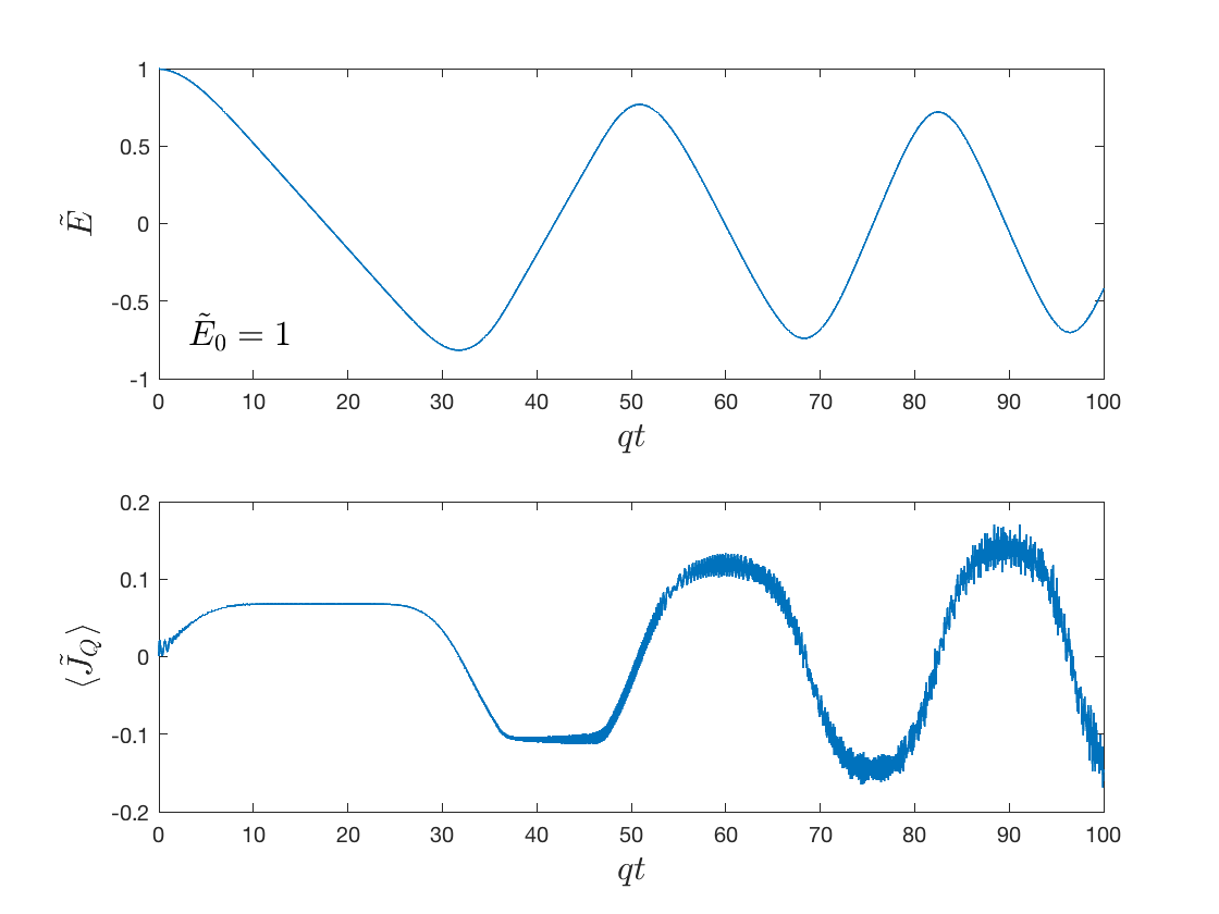
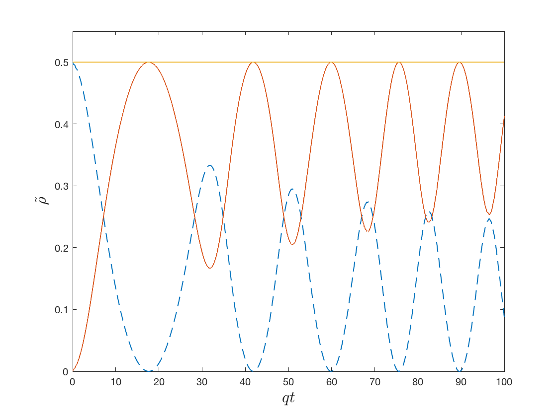
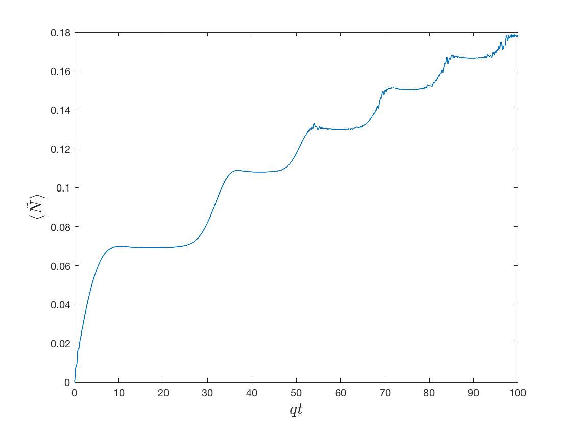
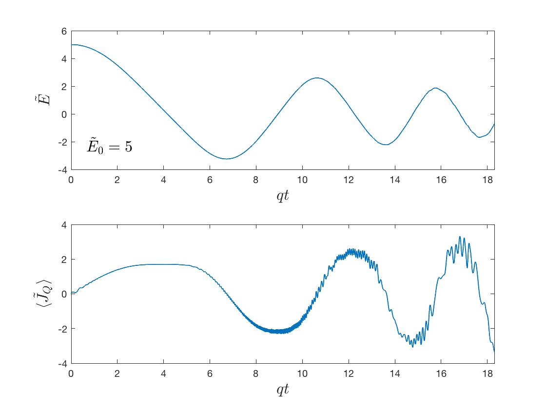
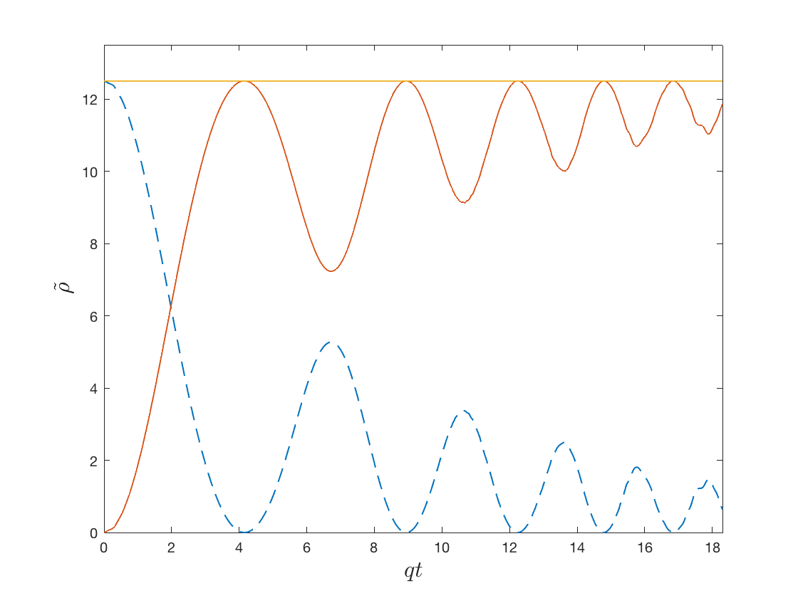
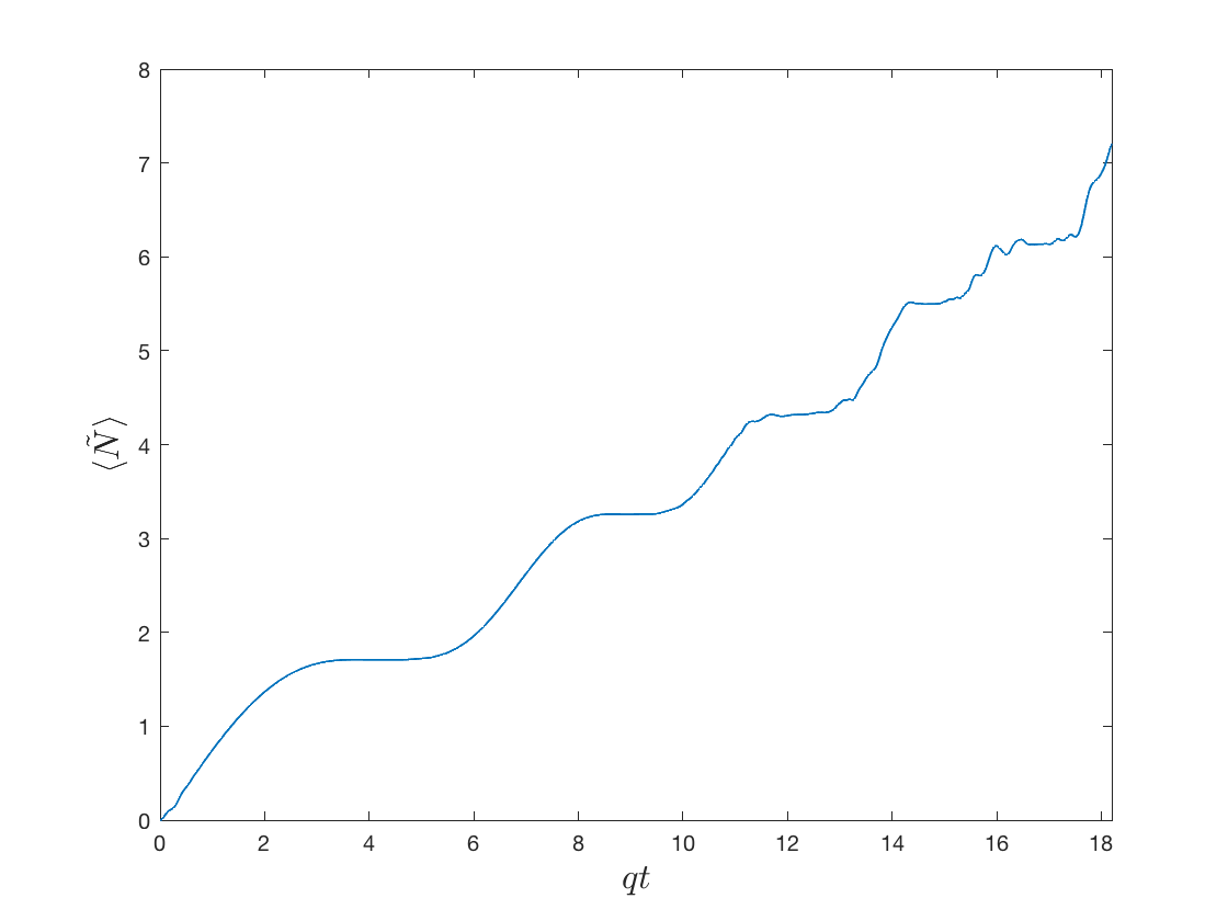
Figure 1: Various quantities are plotted for solutions to the semiclassical backreaction equations for a quantized scalar field with the classical current profile $J_{C}=-E_{0}\,\delta(t)$. The solutions for $\tilde{E}_{0}=1$ are shown across the top row of panels and those for $\tilde{E}_{0}=5$ are shown across the bottom row. The mass of the scalar field is $\frac{m^{2}}{q^{2}}=10$ and thus $\frac{E_{0}}{q}=10$ and $50$ respectively. In the left panels the electric field $\tilde{E}$ and the electric current $\langle\tilde{J}_{Q}\rangle_{\rm ren}$ are plotted. For each of the middle panels the blue dashed curve corresponds to the energy density of the electric field $\rho_{elec}$, the orange solid curve represents the energy density of the created particles $\langle\tilde{\rho}\rangle_{\rm ren}$, and the straight yellow line is the total energy density of the system. The total particle number $\langle\tilde{N}\rangle$ is plotted in the right panels.

In Fig. 2, some of our results for a spin-$\frac{1}{2}$ field coupled to the electric field are shown for $E_{0}=E_{\rm crit}$ in the top panels and $E_{0}=5E_{\rm crit}$ in the bottom ones. Comparing Fig. 2 with Fig. 1, one finds that for the smaller value of the initial electric field, $E_{0}=E_{\rm crit}$, all of the details are very similar to the scalar field case. For the larger initial value of the electric field many of the general features are also similar including the initial damping of the electric field and subsequent plasma oscillations. However, some of the details differ significantly. Due to Pauli blocking the particle production for the spin-$\frac{1}{2}$ field effectively shuts off fairly early in the process. One result is that there is less energy permanently transferred to the particles than in the scalar field case.

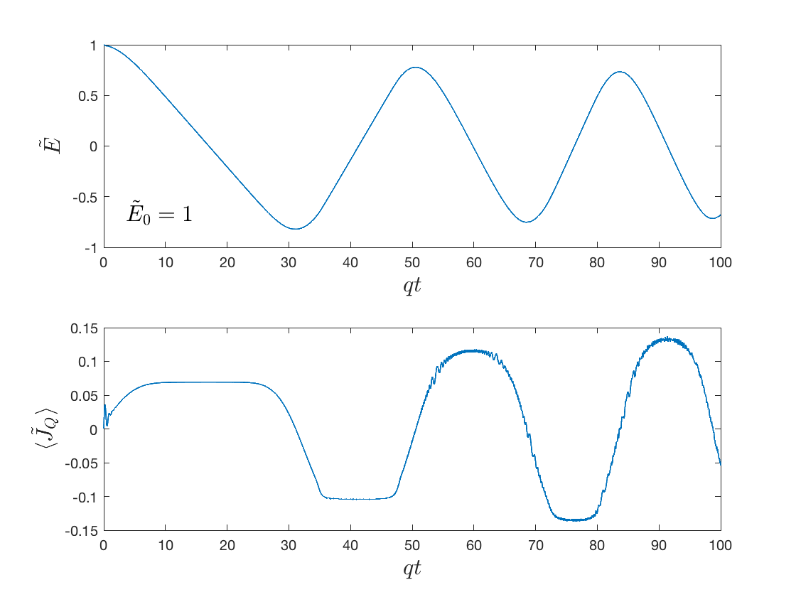
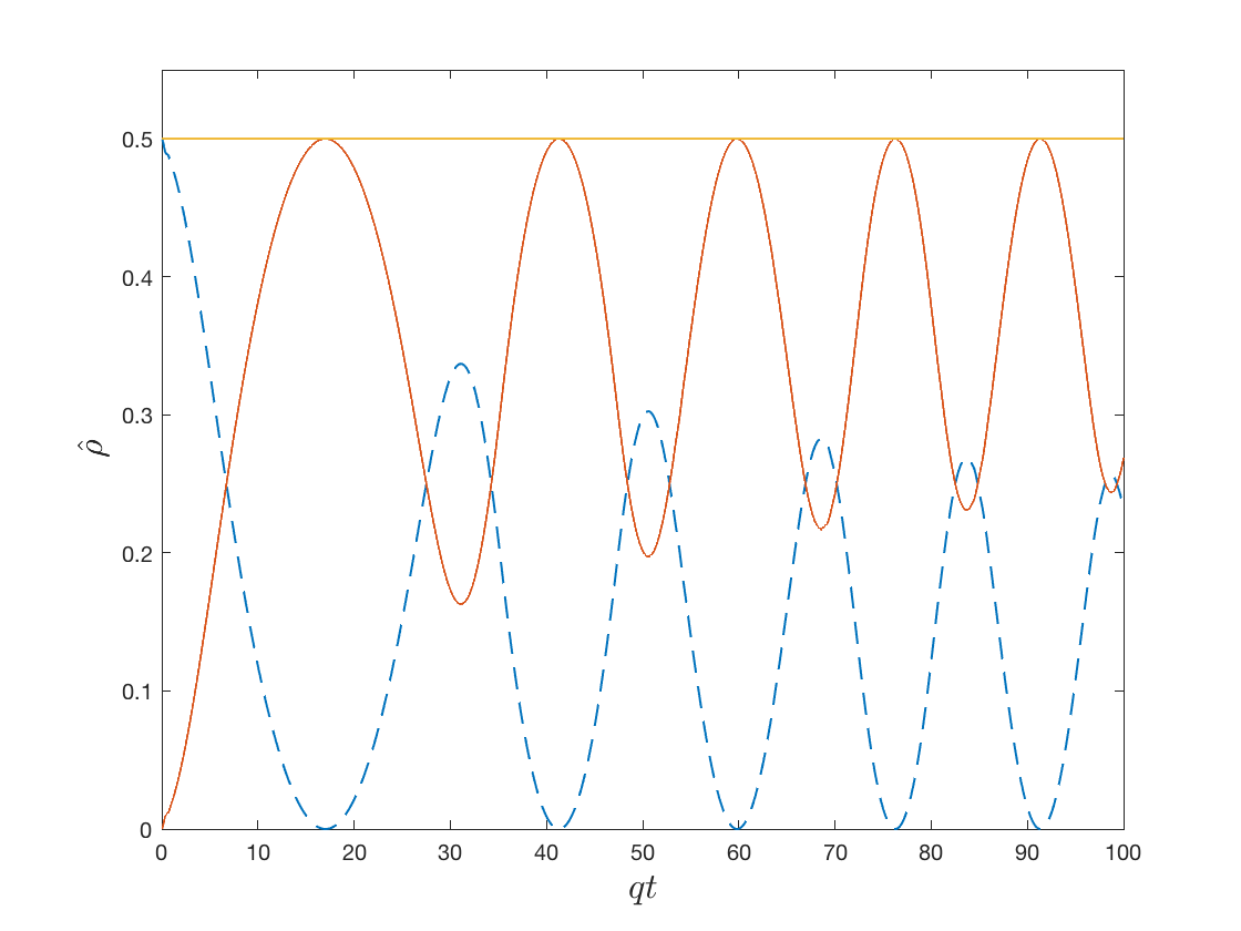
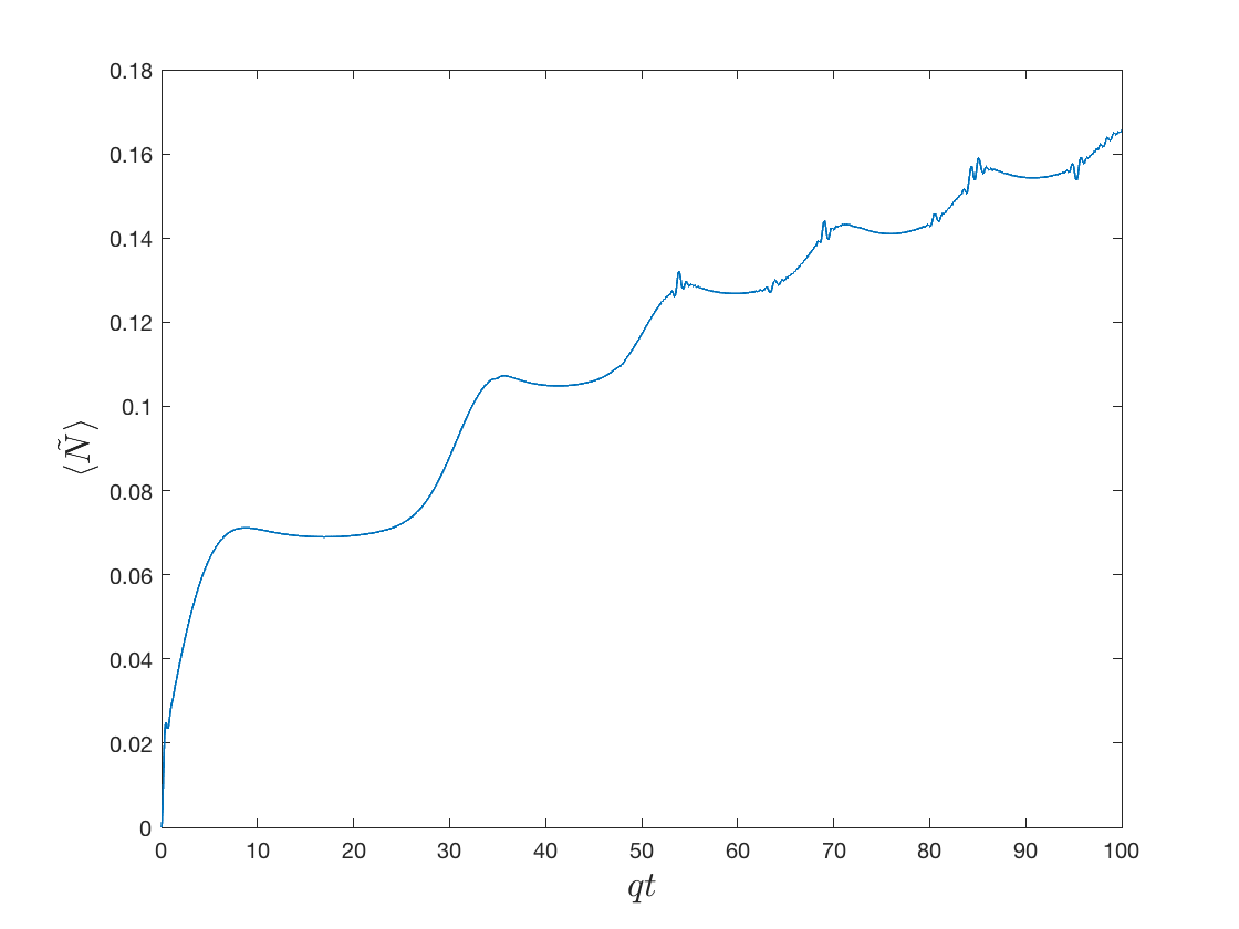
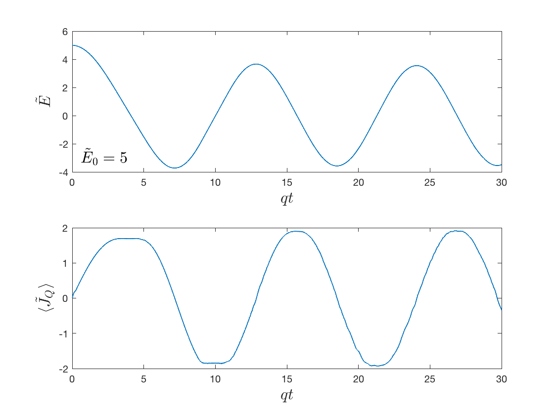
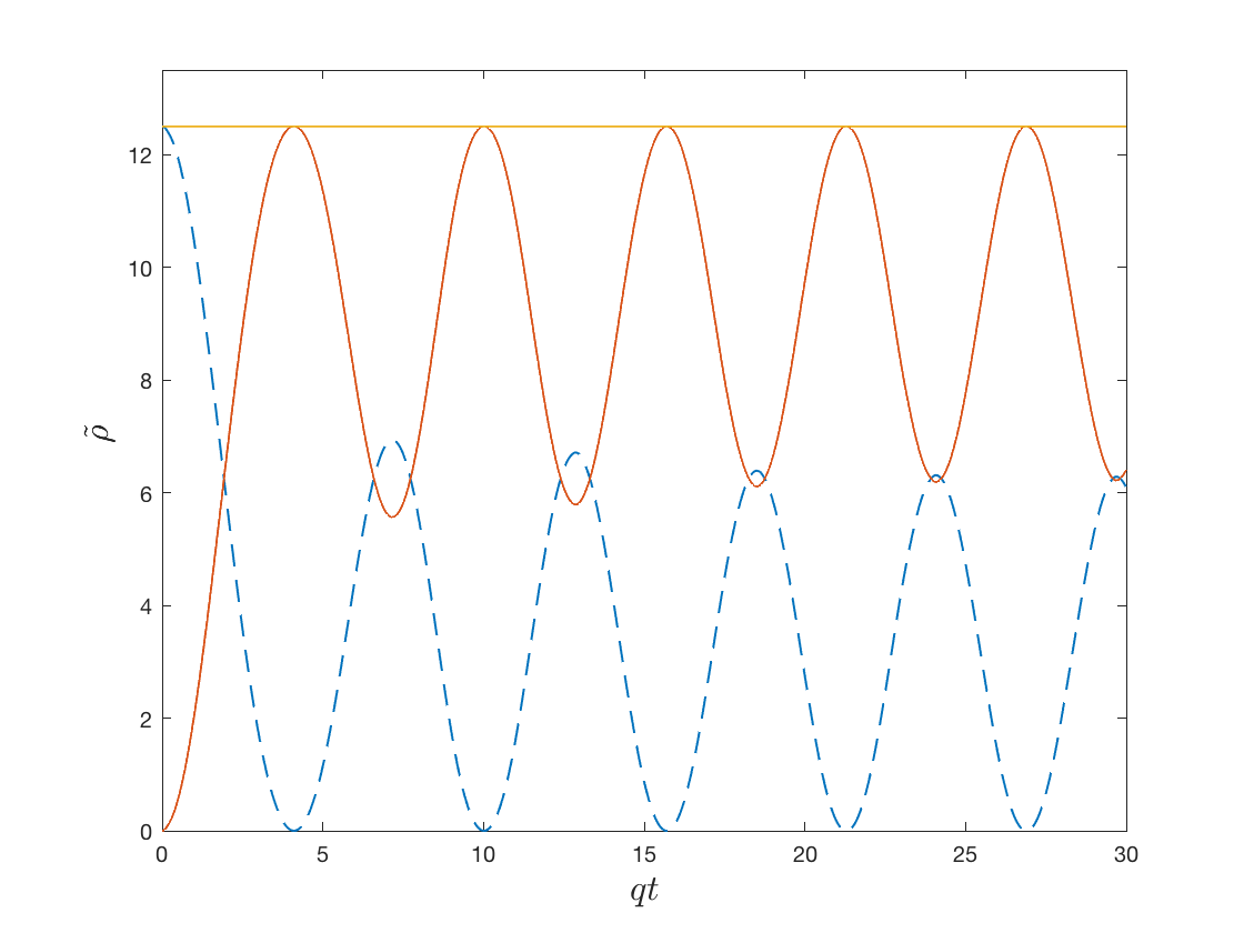
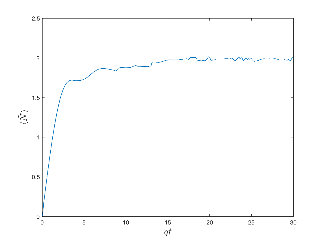
Figure 2: Various quantities are plotted for solutions to the semiclassical backreaction equations for a quantized spin-$\frac{1}{2}$ field with the classical current profile $J_{C}=-E_{0}\,\delta(t)$. The structure of the figure, and also the initial conditions for the electric profile, are the same than in Figure 1.

There are some differences in both the scalar field and spin-$\frac{1}{2}$ cases between the solution for which the electric field is at the critical value initially and the solution for which it is initially much larger. As would be expected there is significantly more particle production and a significantly faster initial damping for the larger field. Once the plasma oscillations begin there also appears to be a much faster approach of the amplitude of the electric field and the total number of particles to their asymptotic values when the initial electric field is larger. Further, examination of the energy density shows that a significant amount of the initial energy of the larger electric field is permanently transferred to the particles during the first damping phase and this increases during the plasma oscillation phase. For the smaller field less energy is transferred initially to the particles during the first damping phase and the permanent transfer of energy to the particles upon each plasma oscillation is smaller.

For both the scalar and spin-$\frac{1}{2}$ fields, a clear correlation is found between the maxima of the energy density of the created particles and the maxima and minima of the current due to the created particles. For cases in which the total number of particles continues to increase significantly after the first burst of particle production, the maxima in the energy density of the created particles correlate with the middles of the time periods when the total number of particles is approximately constant. As expected, the minima of the energy densities of the created particles correspond to times when a new round of significant particle production is just beginning in cases where there is significant particle production after the first burst. In general the periods of significant particle production correspond to periods when energy is being transferred to the particles. It is interesting to note that the above results, obtained within the adiabatic renormalization prescription in the continuous limit, are compatible with the results obtained using a similar method in $3+1$D Tanji as well as those obtained in $1+1$D and/or $3+1$D using lattice simulations lattice-1 ; lattice-2 and classical statistical field theory techniques stat-FT .

It was shown in Refs. and-mot-I ; dunne-part-prod ; and-mot-san that a single particle creation event occurs for an individual mode if the background electric field is either constant or approximately constant. What is different here is that the backreaction of the produced particles produces plasma oscillations. The resulting oscillations of the electric field lead to some modes undergoing multiple particle creation events and sometimes also particle destruction events. This can be seen in Fig. 3 where the time evolution of the function $|\beta_{k}|^{2}$ for $\tilde{E}_{0}=1$ is shown for both the scalar field and spin-$\frac{1}{2}$ field cases. Comparison with the plot of the vector potential $A(t)$ shows that the creation, or destruction, process for an individual mode $k$ happens when $k-qA(t)\approx m$.

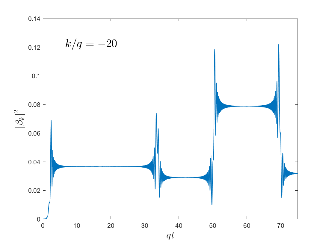
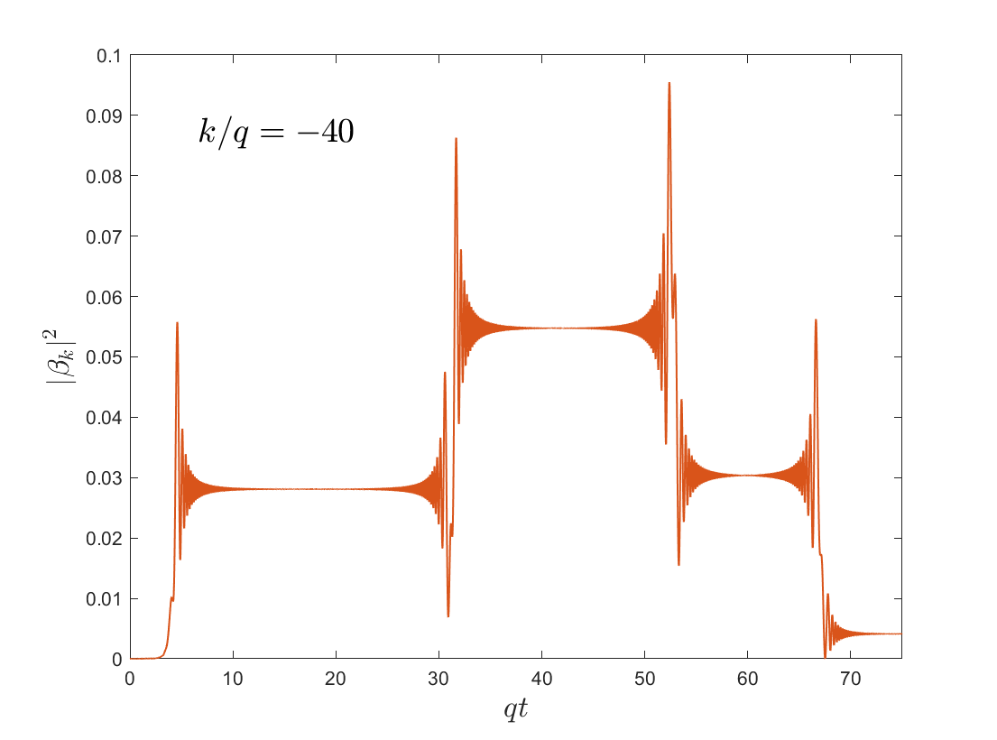
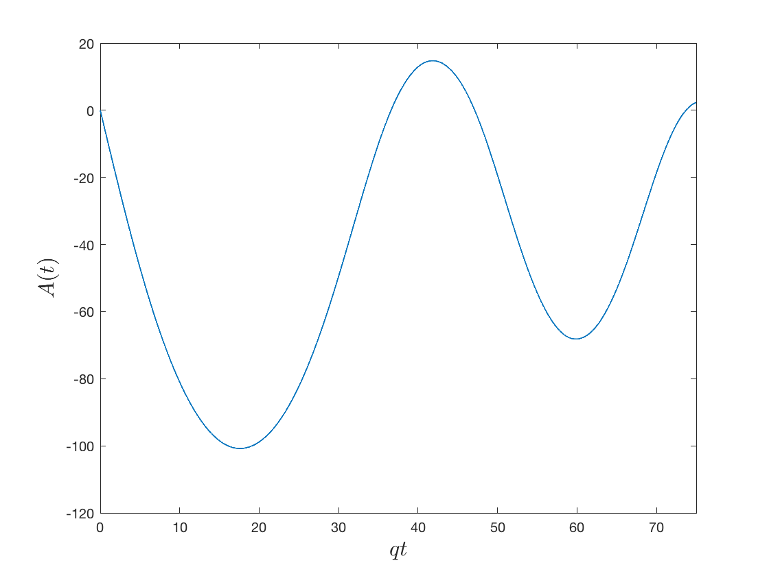
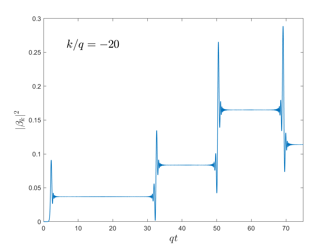
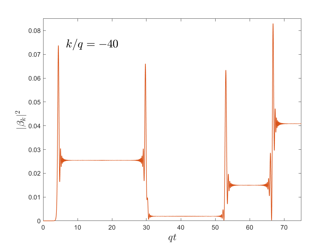
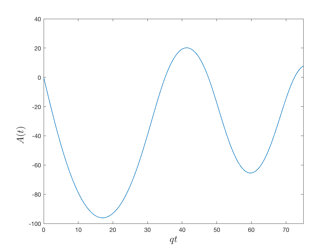
Figure 3: The time-dependent particle number is shown for individual modes when $\tilde{E}_{0}=1$ for the scalar field (top row) and spin-$\frac{1}{2}$ (bottom row) cases for the classical current profile $J_{C}=-E_{0}\,\delta(t)$. The mass of the scalar field is $\frac{m^{2}}{q^{2}}=10$ and thus $\frac{E_{0}}{q}=10$. The vector potential is plotted in the far right panels. For each row the first panel on the left shows the particle number for $\frac{k}{q}=-20$ and the middle panel shows the particle number for $\frac{k}{q}=-40$.

III.2 Massless limit for the spin-$\frac{1}{2}$ field

For completeness we extend our analysis to the massless limit for the spin-$\frac{1}{2}$ field. In this case, the mode equations (18a) and (18b) decouple, and with the initial conditions given in Eq. (42), their solutions are given by

$$h^{I,II}_{k}(t)=\pm\theta(\mp k)e^{\pm i\int^{t}_{t_{0}}(k-qA(t^{\prime}))dt^{\prime}}\quad,$$ (46)

where $\theta(x)$ is the Heaviside step function. The electric current $\langle J_{Q}\rangle_{\rm ren}$ has the simple form given in Eq. (27), and hence, the semiclassical Maxwell equation (19) turns out to be the equation of a harmonic oscillator $\ddot{A}(t)+\frac{q^{2}}{\pi}A(t)=0$. With the initial conditions $E(0)=E_{0}$ and $A(0)=0$, we immediately find the analytic solution $E(t)=E_{0}\cos(\frac{|q|}{\sqrt{\pi}}t)$. The energy density (29) and the number of the created particles are $\langle\rho(t)\rangle_{\rm ren}=\frac{q^{2}}{2\pi}A^{2}(t)$ and $\langle N(t)\rangle=\frac{|qA(t)|}{\pi}$. For a detailed analysis of the adiabatic invariance of the particle number see Ref. BFNP . As in the general case, the total energy of the system is conserved. We note the exact analytic solubility of the case $m=0$ is due entirely to the axial anomaly in $1+1$D. In fact, the constant $\frac{|q|}{\sqrt{\pi}}$ is the mass of the “photon” in the Schwinger model generated by radiative corrections Schwingermass . In the massless case the (nonlocal) effective action $\Gamma[A_{\mu},J_{C}]$ can be obtained exactly and it describes a gauge-invariant vector field with mass $\frac{|q|}{\sqrt{\pi}}$ (see, for instance, Ref. Dash ). The semiclassical calculation of the produced energy due to the external source provides an accurate result. In the massive case the effective action does not describe an integrable model coleman-1 ; gross and the semiclassical picture is expected to break down at some point. The validity of the semiclassical approximation for massless and massive spin-$\frac{1}{2}$ fields for the asymptotically constant classical profile is addressed in Sec. V.1.

IV Validity criterion for the semiclassical approximation

The semiclassical backreaction equation can be derived from Eq. (1) via a loop expansion qftbook . In this case when solving the semiclassical backreaction equation, the semiclassical approximation breaks down if contributions from the quantum terms to the equations become comparable to that of the classical background field and any other classical fields. The reason is that one expects higher-order terms in the loop expansion to be important in that limit. However, there is a different way to derive the semiclassical backreaction equation called the large-$N$ expansion. In this expansion one considers $N$ identical quantum fields coupled to the background field, which to leading order is treated as a classical field. At next-to-leading order in the large-$N$ expansion, quantum effects due to the background field first appear large-N-1994 ; hu-verdaguer . Thus in this expansion it is consistent to consider solutions to the semiclassical backreaction equation for which the quantum fields have a significant effect on the classical background field. Here we will take $N=1$ and consider a wide range of situations ranging from those where the background electric field is small compared with the (Schwinger) critical scale $E_{\rm crit}\equiv m^{2}/q$ and quantum effects are correspondingly small to those where the background electric field is large compared to the critical value and quantum effects are correspondingly large. The critical value is the threshold for which a significant amount of particle production is expected to occur.

The large-$N$ expansion provides a formal framework for the semiclassical backreaction equation when quantum effects are significant. However, it does not guarantee that the semiclassical approximation is valid. There are three reasons. The first is that interactions of the quantum fields which are coupled to the classical background field are ignored in most cases, including those considered here. This works if the interactions are small over the time scales relevant to the problem. The second is that even if the next-to-leading order terms in the large-$N$ expansion are initially small in size, it has been shown in certain quantum mechanics calculations that they undergo secular growth fred1 and there is evidence that secular growth also occurs for such terms in quantum field theory fred-emil-private . However, there is also evidence that partial resummations of certain classes of Feynman diagrams eliminate this problem fred2 ; fred3 . The third is that the semiclassical backreaction equation involves an expectation value of some quantity such as the electric current or stress-energy tensor that is constructed from the quantum fields. For an expectation value to be a good approximation to what one would measure in quantum theory, it is necessary that quantum fluctuations are small.

A natural way to estimate the size of quantum fluctuations is to evaluate the two-point correlation function for the current. There are several different two-point correlation functions including (i) $\langle J(t,x)J(t^{\prime},x^{\prime})\rangle$, (ii) the connected part, i.e., $\langle J(t,x)J(t^{\prime},x^{\prime})\rangle-\langle J(t,x)\rangle\langle J(t^{\prime},x^{\prime})\rangle$, (iii) the time-ordered correlation function $\langle T(J(t,x)J(t^{\prime},x^{\prime}))\rangle$, etc. There are problems associated with some of these, as described in Refs. wu-ford ; phillips-hu ; validitygravity . For example, it has been shown for the symmetric part of the stress-energy tensor two-point correlation function that there can be state-dependent divergences in the limit that the points come together wu-ford . A related issue is that it has been shown in at least one case in the limit that the points come together that different renormalization schemes can give different results for a particular quantity made from one component of the stress-energy tensor two-point correlation function phillips-hu . There can also be covariance issues with some of the quantities made from the stress-energy tensor two-point correlation function validitygravity .

There is a correlation function that is free of these problems and which emerges naturally from the semiclassical theory itself and that is $\langle[J(t,x),J(t^{\prime},x^{\prime})]\rangle$. By perturbing the semiclassical backreaction equation one is led to the so-called linear response equation which contains this correlation function and which describes the time evolution of perturbations about a given semiclassical solution. A criterion was developed in Ref. validitygravity for the validity of the semiclassical approximation in gravity which states that a necessary condition for the validity of the semiclassical approximation to be valid is that any linearized, gauge-invariant scalar quantity constructed from solutions to the linear response equations with finite nonsingular initial data should not grow without bound. It is important to emphasize that this is not a sufficient condition for the validity of the semiclassical approximation. The criterion was adapted to cover preheating during chaotic inflation validitypreheating where a significant amount of particle production occurs and quantum effects are large. If the criterion is applied to semiclassical quantum electrodynamics then it would state that the semiclassical approximation breaks down if any linearized gauge-invariant quantity constructed from solutions to the linear response equation with finite nonsingular initial data grows rapidly for some period of time.

IV.1 Linear response equation

The linear response equation for semiclassical electrodynamics can be obtained by perturbing Eq. (19) about a background solution to the semiclassical equation with the result

$$\frac{d^{2}}{dt^{2}}\delta A(t)=-\frac{d}{dt}\delta E=\delta J_{C}+\delta\langle J_{Q}\rangle\quad.$$ (47)

It can be seen from Eq. (47) that a first integral of the linear response equation gives the perturbed electric field, which is gauge invariant.

To analyze the behaviors of solutions to this equation, particularly at early times, it is useful to break the solutions to the semiclassical backreaction equation into two parts with

$$E_{Q} \equiv E-E_{C}\quad,$$ (48a)

$$E_{C} \equiv -\int_{t_{0}}^{t}dt_{1}\,J_{C}(t_{1})\quad.$$ (48b)

From the structure of the linear response equation it is clear that its solutions $\delta E$ can be broken up in exactly the same way. Then, the criterion for the validity of the semiclassical approximation can be modified to state that if the quantity $\delta E_{Q}$ grows significantly during some period of time then the semiclassical approximation is invalid. It is worth noting that because $\langle J_{Q}\rangle$ and $\delta\langle J_{Q}\rangle$ are constructed from solutions to the mode equation which depend on the vector potential $A$, and therefore indirectly on $E$, then $E_{Q}$ depends on $E_{C}$ and $\delta E_{Q}$ depends on $\delta E_{C}$.

In Appendix A it is shown for both the scalar and spin-$\frac{1}{2}$ coupled systems that for homogeneous perturbations, $\delta\langle J_{Q}\rangle$ depends upon the two-point correlation function for the current. A more general derivation is given in Ref. kubostuff . For scalar fields the result is

$$\delta\langle J_{Q}\rangle_{\rm ren}=-\frac{q^{2}}{\pi}\delta A(t)\int_{-\infty}^{\infty}dk\,\bigg{(}|f_{k}(t)|^{2}-\frac{m^{2}}{2\omega^{3}}\bigg{)}+\,i\int_{-\infty}^{\infty}dx^{\prime}\int_{-\infty}^{t}dt^{\prime}\,\langle[J_{Q}(t,x),J_{Q}(t^{\prime},x^{\prime})]\rangle\,\,\delta A(t^{\prime})\quad,$$ (49)

where

$$\omega\equiv\sqrt{m^{2}+k^{2}}\quad,$$ (50)

and

$$\int_{-\infty}^{\infty}dx^{\prime}\langle[J_{Q}(t,x),J_{Q}(t^{\prime},x^{\prime})]\rangle=\frac{4\,i\,q^{2}}{\pi}\int_{-\infty}^{\infty}dk\bigg{(}k-qA(t)\bigg{)}\bigg{(}k-qA(t^{\prime})\bigg{)}\textnormal{Im}\bigg{\{}f_{k}(t)^{2}f_{k}^{*}(t^{\prime})^{2}\bigg{\}}\quad.$$ (51)

It can be shown, using the point-splitting technique, that the divergence structure in the first integral is conveniently compensated for by the divergence structure that is inherent in the second integral. Therefore, $\delta\langle J_{Q}\rangle$ is finite and the overall equation is well defined.

For spin-$\frac{1}{2}$ fields the renormalized perturbation of the quantum current in (47) is

$$\delta\langle J_{Q}\rangle_{\rm ren}=-\frac{q^{2}m^{2}}{2\pi}\delta A(t)\int_{-\infty}^{\infty}\frac{dk}{\omega^{3}}+\,i\int_{-\infty}^{\infty}dx^{{}^{\prime}}\int_{-\infty}^{t}dt^{{}^{\prime}}\langle[J_{Q}(t,x),J_{Q}(t^{{}^{\prime}},x^{{}^{\prime}})]\rangle\,\delta A(t^{{}^{\prime}})\quad,$$ (52)

with

$$\int_{-\infty}^{\infty}dx^{\prime}\langle[J_{Q}(t,x),J_{Q}(t^{{}^{\prime}},x^{{}^{\prime}})]\rangle=\frac{4i\,q^{2}}{\pi}\int_{-\infty}^{\infty}dk\,\textnormal{Im}\bigg{\{}h_{k}^{I}(t)h_{k}^{II}(t)h_{k}^{I*}(t^{\prime})h_{k}^{II*}(t^{\prime})\bigg{\}}\;.$$ (53)

Recall that in the massless limit we find that the mode equations decouple and the solutions are given in Eq. (46). Thus, for a given value of $k$ either $h^{I}_{k}$ or $h^{II}_{k}$ is zero, and hence $h^{I}_{k}h^{II}_{k}=0$ for any value of $k$. Therefore in the massless limit the current-current commutator in Eq. (53) is zero.

IV.2 Approximate solutions to the linear response equation

From Eqs. (47), (49), and (52), it is clear that the linear response equation is an integro-differential equation. This makes it significantly more difficult to solve numerically compared to an ordinary differential equation. A useful way to approximate the solutions to the linear response equation for the case of homogeneous perturbations was given in Ref. validitypreheating . It involves solving the semiclassical backreaction equation for two sets of initial conditions which differ from each other by only a small amount. At early times we expect these two solutions to be an approximate solution to the linear response equation so long as the difference does not grow too large. If this difference grows significantly, then the corresponding solution to the linear response equation should also grow substantially. Hence, our criterion for the validity of the semiclassical approximation is considered to be violated.

As has been mentioned previously, solutions to the semiclassical backreaction equation tend to oscillate over long periods of time due to plasma oscillations and it is possible that solutions to the linear response equation could oscillate over shorter periods of time. While there is no problem in comparing the absolute difference between two solutions to the semiclassical backreaction equation, it is more problematic when one considers the relative difference because the denominator will vanish at certain points. For this reason we introduce a modified version of the relative difference which is guaranteed to be no smaller than zero and no larger than one. Consider two solutions to either the classical or semiclassical backreaction equation in 1+1D, $\vec{E}_{1}=E_{1}\hat{x}$ and $\vec{E}_{2}=E_{2}\hat{x}$ (or just $E_{1}$ and $E_{2}$ since we are only considering one spatial dimension). Then the absolute and relative differences are respectively

$$\Delta E \equiv E_{2}-E_{1}\quad,$$ (54a)

$$R \equiv \frac{|\Delta E|}{|E_{1}|+|E_{2}|}\quad.$$ (54b)

We note that $R$ can be easily reexpressed as a Lorentz-invariant quantity.

It is useful to apply the relative difference $R$ for two solutions to the classical backreaction equation which, as can be seen in Eq. (48b), are simply integrals over the classical current $J_{C}$. Consider a classical current of the form

$$J_{C}=-E_{0}\,\dot{g}(t)\quad.$$ (55)

Here $\dot{g}(t)$ is the time derivative of some well-behaved, dimensionless function $g(t)$, and the solution to the classical Maxwell equation is $E_{C}=E_{0}g(t)$. In the following sections we will consider the cases $g(t)=\frac{qt}{1+qt}$ and $g(t)=\sech^{2}(qt)$, with the latter being the Sauter pulse. The solutions are parametrized by the constant $E_{0}$. For two solutions to Eqs. (48b) with (55), $E_{C1}$ and $E_{C2}$, with $E_{0}=E_{01}$ and $E_{0}=E_{02}$ respectively, we have for the absolute and relative difference

$$\Delta E_{0} \equiv E_{02}-E_{01}\quad,$$ (56a)

$$R_{C} = \frac{|\Delta E_{C}|}{|E_{C1}|+|E_{C2}|}=\frac{|\Delta E_{0}|}{|E_{01}|+|E_{02}|}\quad.$$ (56b)

Next, consider two solutions to the semiclassical backreaction equation. Since we are considering classical currents, which are zero initially, and an electric field that is zero initially, there is no ambiguity in the choice of vacuum state. Therefore these solutions are also parametrized by the value of $E_{0}$ for a given function $g(t)$. Using the subscripts $1$ and $2$ to denote quantities computed for these solutions, it is clear that the difference $\Delta E$ is an exact solution to the equation

$$-\frac{d\Delta E}{dt}=\Delta J_{C}+\Delta\langle J_{Q}\rangle\quad.$$ (57)

with $\Delta J_{C}=J_{C2}-J_{C1}$ and $\Delta\langle J_{Q}\rangle=\langle J_{Q2}\rangle-\langle J_{Q1}\rangle$.

Suppose at some early time $t_{1}$, when $E_{C}$ is still very small with no significant amount of particle production, that $R_{C}(t_{1})\ll 1$. One can then arrange the initial conditions for the perturbation $\delta E$ such that $\delta E(t_{1})=\Delta E(t_{1})$. It is also obvious that one can set for all times $\delta J_{C}(t)=\Delta J_{C}(t)$. Then Eq. (57) is approximately equivalent to the linear response equation (47) so long as $\Delta\langle J_{Q}\rangle\approx\delta\langle J_{Q}\rangle$, which one would certainly expect to be the case at times near $t_{1}$.

As discussed in the previous subsection [see Eq. (48a)], it is more useful at early times to consider the quantity $\Delta E_{Q}\approx\delta E_{Q}$. To measure the relative growth of $\Delta E_{Q}$ we compute the relative difference

$$R_{Q}=\frac{|\Delta E_{Q}|}{|E_{Q1}|+|E_{Q2}|}\;.$$ (58)

This difference can then be compared to the relative difference between the corresponding classical solutions $R_{C}$ in Eq. (56b), which does not change in time.

Consider two times $t_{2}>t_{1}$ where $t_{1}$ is the initial time discussed above when one imagines fixing the starting values for the linear response equation and $t_{2}$ is a relatively early time after that. Then the possibilities are as follows. (i) If $R_{Q}(t)\lesssim R_{C}$ then the criterion for the validity of the semiclassical approximation will be satisfied by the approximate homogeneous solutions that we consider up to the time $t_{2}$. (ii) If for any times between $t_{1}$ and $t_{2}$, $R_{Q}(t)\gg R_{C}$, then the solution to the linear response equation, $\delta E$, grows rapidly during at least some part of the period $t_{1}\leq t\leq t_{2}$ and the criterion for validity of the semiclassical approximation is not satisfied. Note that once the semiclassical approximation has broken down, one can no longer trust its solutions even if for later times $R_{Q}\lesssim R_{C}$. (iii) Finally, the intermediate case when $R_{Q}$ is larger than $R_{C}$ but still of the same order of magnitude is ambiguous. Perhaps the best that can be said is in this case quantum fluctuations are increasing and so the accuracy of the semiclassical approximation is decreasing in proportion to this increase.

V Numerical Results

In this section we implement a numerical analysis to study the validity of the semiclassical approximation for two different classical source profiles. To do so, we use the method described in the previous section to compare the numerical solutions of the semiclassical backreaction equation for two distinct, but very close values of the external source amplitude $E_{0}$. The first profile considered has a classical source current given by

$$J_{C}=-\frac{qE_{0}}{(1+qt)^{2}}\quad,$$ (59)

for $t\geq 0$ and $J_{C}=0$ for $t<0$. The classical solution of the Maxwell equation ($-\dot{E}_{C}=J_{C}$) gives rise to the asymptotically constant electric field profile for $t\geq 0$

$$E_{C}(t)=E_{0}\left(\frac{qt}{1+qt}\right)\quad.$$ (60)

The second profile considered is the Sauter pulse with source current given by

$$J_{C}=2qE_{0}\textnormal{sech}^{2}(qt)\textnormal{tanh}(qt)\quad,$$ (61)

and corresponding classical electric field

$$E_{C}(t)=E_{0}\textnormal{sech}^{2}(qt)\quad.$$ (62)

In Fig. 4 we show the classical behavior of both profiles. For the first profile, one can easily see that at late times the electric field approaches the constant value $E_{0}$. The Sauter pulse models a possibly more realistic scenario for the detection of the Schwinger effect, in which both the initial and the final values of the classical electric field tend to zero. Note that, for the first profile we choose an initial time $t_{0}=0$, while for the Sauter pulse the initial time has to be fixed as $t_{0}=-\infty$.

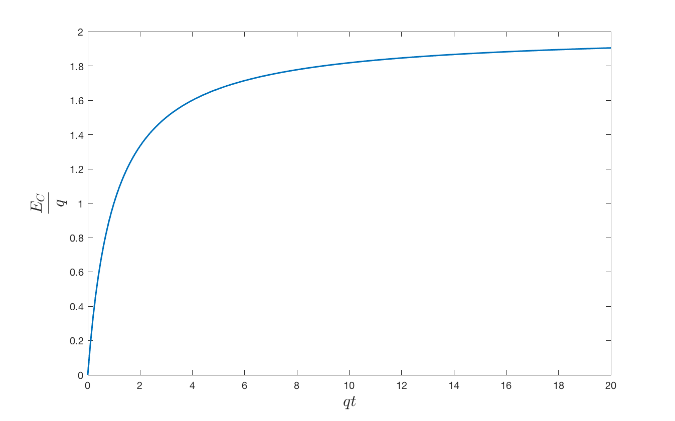
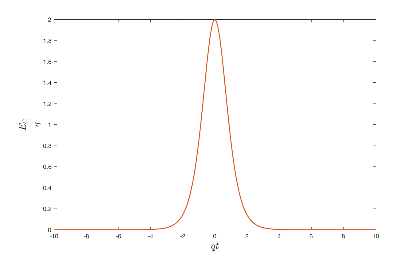
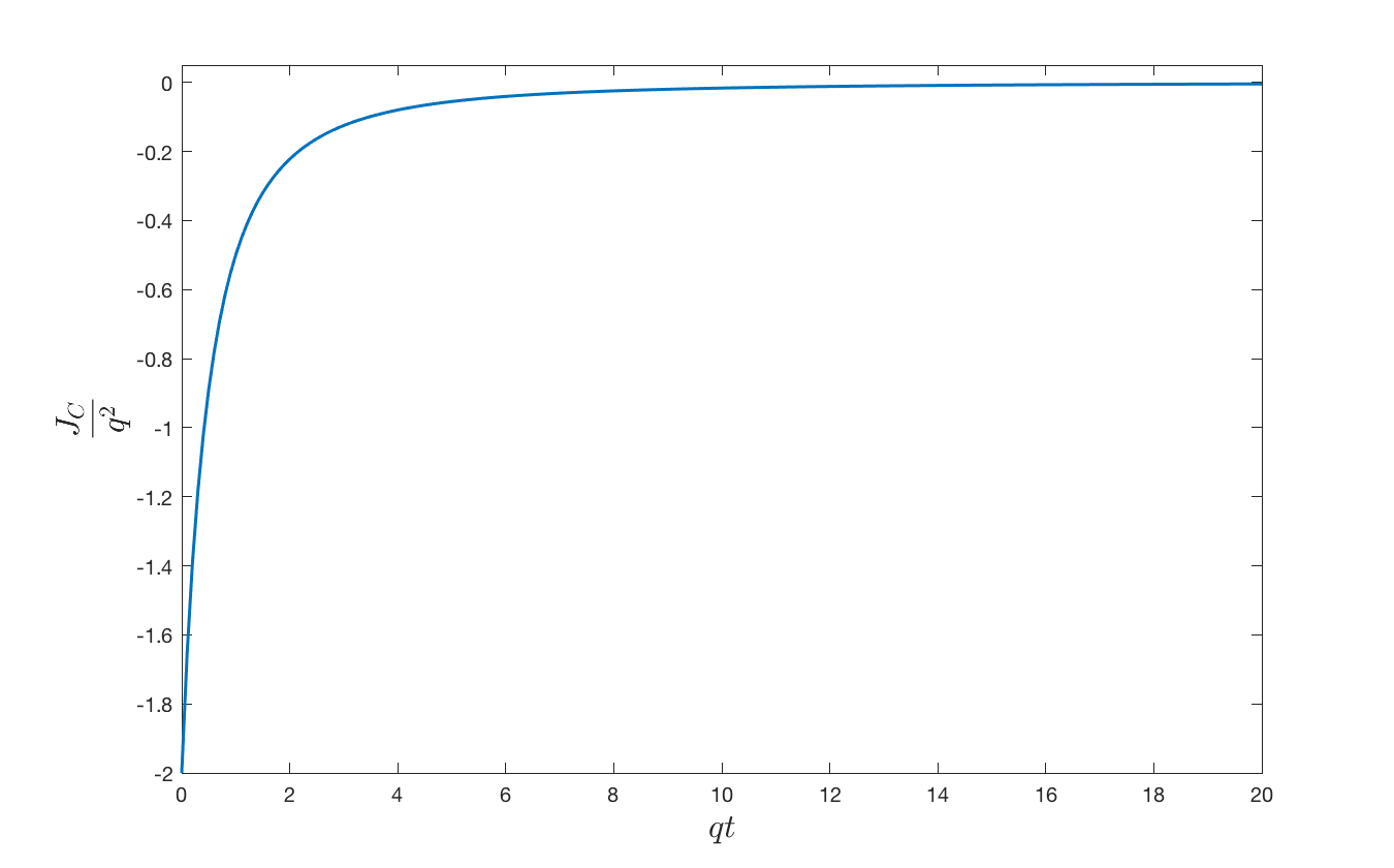
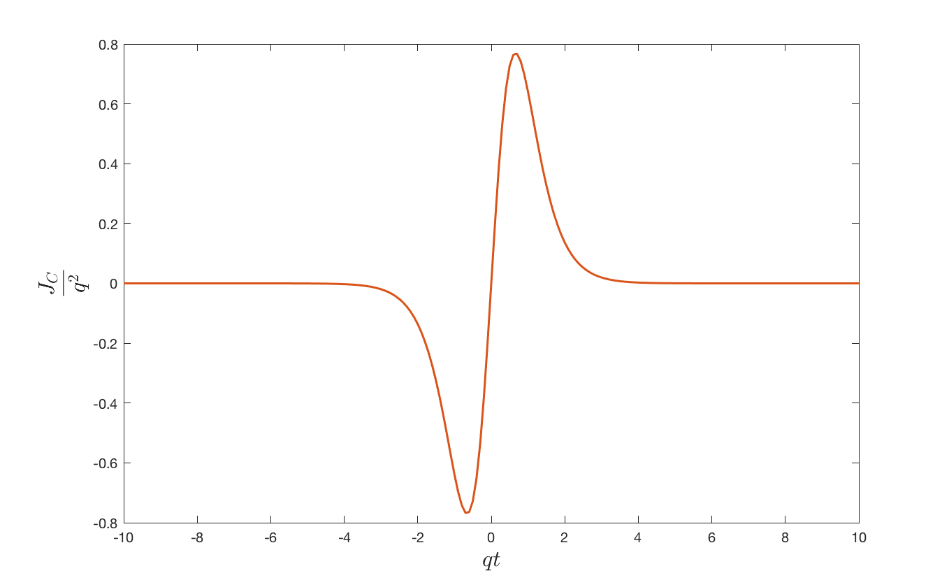
Figure 4: Electric profiles for $E_{0}/q=2$. In the left (top) panel we show the asymptotically constant profile. In the right (top) panel we show the Sauter pulse. In both bottom panels, the classical current generating the respective electric field profiles is plotted. For the asymptotically constant profile we choose an initial time $t_{0}=0$, while for the Sauter pulse the initial time has to be fixed as $t_{0}=-\infty$.

As discussed in Sec. IV.2, it is useful, particularly at early times, to work with the quantity $E_{Q}$ in Eq. (48a) which is the difference between the net electric field and the electric field $E_{C}$ that would be present if there were no quantum effects. Therefore the natural quantity to consider is the relative difference $R_{Q}$ in Eq. (58) which is constructed from two solutions to the semiclassical backreaction equation with values of $E_{0}$ that differ by some small amount. This can be compared to the relative difference $R_{C}$ between two solutions to the classical Maxwell equation with the same values of $E_{0}$.

In what follows, numerical results will be shown for calculations of $R_{Q}$ and other quantities such as $E(t)$, $\langle J_{Q}\rangle$, and $\langle N\rangle$ for scalar and spin-$\frac{1}{2}$ semiclassical electrodynamics for the asymptotically constant classical profile and then for the Sauter pulse classical profile. As stressed before, we mainly focus on the early-time behavior. In both cases it is assumed that the electric field and vector potential are initially zero. As a result, for scalar fields the initial conditions for the mode functions are

$$f_{k}(t_{0})=\frac{1}{\sqrt{2\omega}}\quad,\quad\dot{f}_{k}(t_{0})=-i\sqrt{\frac{\omega}{2}}\quad.$$ (63)

For spin-$\frac{1}{2}$ fields the initial conditions are

$$h_{k}^{I}(t_{0})=\sqrt{\frac{\omega-k}{2\omega}}\quad,\quad h_{k}^{II}(t_{0})=-\sqrt{\frac{\omega+k}{2\omega}}\quad.$$ (64)

First, we discuss the mass dependence of the function $R_{Q}$ and its relation to the validity of the semiclassical approximation, with a focus on the asymptotically constant profile. Then, we show the results of our analysis for the most relevant case $E_{0}\sim E_{\rm crit}=m^{2}/q$ for both the asymptotically constant profile and the Sauter pulse. As in Sec. III, for the numerical computations we use the dimensionless parameters described therein. However, in this section the electric field and the electric current are given in terms of $E/q$ and $J/q^{2}$ respectively.

Since we are considering multiple cases and subcases, a summary of all relevant information, including all cases and sub-cases with figure references, can be found in Table 1.

Quantum Field	Classical Profile	Mass Cases	Figure Reference
Spin 1/2	Asymptotically Constant	$m^{2}\ll qE_{0}\,\,(\textnormal{or}\,\,m\rightarrow 0)$	6, 7
		$m^{2}\sim qE_{0}$	5, 6, 7, 9
	Sauter Pulse	$m^{2}\ll qE_{0}(\textnormal{or}\,\,m\rightarrow 0)$	N/A
		$m^{2}\sim qE_{0}$	10
Complex Scalar	Asymptotically Constant	$m^{2}\ll qE_{0}\,\,(\textnormal{or}\,\,m\rightarrow 0)$	8
		$m^{2}\sim qE_{0}$	8, 9
	Sauter Pulse	$m^{2}\ll qE_{0}\,\,(\textnormal{or}\,\,m\rightarrow 0)$	N/A
		$m^{2}\sim qE_{0}$	10

Table 1: A table organizing the various cases and subcases that are investigated in the paper. Included are figure references for ease of use. Note that cases with $m^{2}\gg qE_{0}$ are not included; they are discussed in the main text on the basis of the decoupling mechanism.

V.1 Asymptotically constant classical profile

V.1.1 Massless spin-$\frac{1}{2}$ field

As explained in Sec. III.2, for $m=0$ the mode equations (18a) and (18b) decouple, and $\langle J_{Q}\rangle_{\rm ren}=-\frac{q^{2}}{\pi}A$. Thus the semiclassical Maxwell equation (19) reduces to

$$\ddot{A}+\frac{q^{2}}{\pi}A=J_{C}\quad,$$ (65)

which is the equation for a simple harmonic oscillator with frequency $\frac{|q|}{\sqrt{\pi}}$ and external source $J_{C}$. In this case, the linear response equation is just

$$\delta\ddot{A}+\frac{q^{2}}{\pi}\delta A=\delta J_{C}\quad.$$ (66)

Note that $\delta\langle J_{Q}\rangle_{\rm ren}=-\frac{q^{2}}{\pi}\delta A$ and also that the initial conditions for $\delta J_{C}$ can be arranged so that $\delta J_{C}\equiv\Delta J_{C}$.

For the asymptotically constant profile, $J_{C}$ is given in Eq. (59). With initial conditions $A(0)=0$ and $E(0)=0$, we immediately find

$$A(t) = -\frac{E_{0}}{q}\Bigg{[}\cos(\frac{1+qt}{\sqrt{\pi}})\mathrm{Ci}(\pi^{-1/2})-\cos(\frac{1+qt}{\sqrt{\pi}})\mathrm{Ci}\Bigg{(}\frac{1+qt}{\sqrt{\pi}}\Bigg{)}$$

$$\qquad\qquad+\sqrt{\pi}\sin(\frac{qt}{\sqrt{\pi}})+\sin(\frac{1+qt}{\sqrt{\pi}})\mathrm{Si}(\pi^{-1/2})-\sin(\frac{1+qt}{\sqrt{\pi}})\mathrm{Si}\Bigg{(}\frac{1+qt}{\sqrt{\pi}}\Bigg{)}\Bigg{]}\quad,$$

where $\mathrm{Ci}(x)=-\int_{x}^{\infty}\frac{\cos(t)}{t}dt$ and $\mathrm{Si}(x)=\int_{0}^{x}\frac{\sin(t)}{t}dt$ are the cosine and the sine integral functions respectively. Hence, we can conclude that for any two solutions $E_{1}(t)$ and $E_{2}(t)$ with $E_{0}=E_{01}$ and $E_{0}=E_{02}$ respectively, the relation

$$R_{Q}(t)=\frac{|E_{Q1}(t)-E_{Q2}(t)|}{|E_{Q1}(t)|+|E_{Q2}(t)|}=\frac{|E_{01}-E_{02}|}{|E_{01}|+|E_{02}|}=R_{C}\quad,$$ (68)

is always satisfied. Although this result was derived for the asymptotically constant profile (59), it holds for any classical current of the form $J_{C}=-E_{0}g(t)$.

V.1.2 Massive spin-$\frac{1}{2}$ field

We next study the relationship between the behavior of $R_{Q}$, the mass of the spin $\frac{1}{2}$ field, and the value of $E_{0}$ in Eq. (59). As illustrated in our numerical results below, the most important effect on $R_{Q}$ comes from the size of the dimensionless quantity $\frac{qE_{0}}{m^{2}}$. We distinguish between three different cases: (i) $\frac{qE_{0}}{m^{2}}\gg 1$ in which the mass is relatively small compared to the electric field and there is a lot of particle production, (ii) the intermediate case $\frac{qE_{0}}{m^{2}}\sim 1$ where there is a significant amount of particle production, and (iii) $\frac{qE_{0}}{m^{2}}\ll 1$ in which the mass is relatively large compared to the electric field and there is very little particle production.

The beginning of the transition from intermediate to large effective masses is shown in Fig. 5 where various quantities, such as the electric field, are plotted for $E_{0}/q=1$ and $\frac{m^{2}}{q^{2}}=1$ and $\frac{m^{2}}{q^{2}}=2$. As expected, the amount of particle production that occurs decreases significantly as $\frac{qE_{0}}{m^{2}}$ decreases and thus as the effective mass increases. Note that the time scale on which backreaction effects occur increases significantly with an increase in the effective mass.

In the very-large-mass limit $\frac{qE_{0}}{m^{2}}\to 0$, the electric field will not have enough energy to create particles, so one expects that $\langle J_{Q}\rangle_{\rm ren}\to 0$ and $E\to E_{C}$. This is in agreement with the decoupling theorem in perturbative quantum field theory APtheorem . Heavy masses decouple in the low-energy description of the theory, which in this case is purely classical electrodynamics for $m^{2}\to\infty$, with $E_{0}$ fixed.

In the intermediate cases shown in Fig. 5 where $\frac{qE_{0}}{m^{2}}\sim 1$, there is a significant amount of particle production and once enough particle production has occurred the value of $R_{Q}$ starts to increase rapidly, possibly exponentially for $\frac{qE_{0}}{m^{2}}=1$. This rapid rise continues until the backreaction of the particles on the background electric field is strong enough that the electric field has stopped increasing and has begun to noticeably decrease in size. Thus in the intermediate case it appears that our criterion for the validity of the semiclassical approximation is not satisfied due the rapid and significant growth in $R_{Q}$ at relatively early times.

The transition from the intermediate case to the small-effective-mass case when $E_{0}/q=1$ is shown in Fig. 6. Comparison with Fig. 5 shows that the intermediate case extends to $\frac{m^{2}}{q^{2}}=0.1$, but not to $\frac{m^{2}}{q^{2}}=0.01$ which has a qualitatively different behavior. In particular for the relatively small-mass and zero-mass cases the particle production is more rapid and backreaction effects on the electric field are significant after a much smaller amount of time than for intermediate masses. Examination of the behavior of $R_{Q}$ shows that it does not grow rapidly in time for the small-mass case and, as mentioned above, is constant in the massless case. Thus our criterion for the validity of the semiclassical approximation is satisfied by the homogeneous approximate solutions that we consider in the relatively small-mass case.

In the above analysis the value of the ratio $\frac{qE_{0}}{m^{2}}$ has been shown to dictate the different types of qualitative behaviors the solutions have. Of course one can change the values of $qE_{0}$ and $m^{2}$ in ways that keep the ratio fixed. In Figs. 5 and 6, $E_{0}/q=1$. In Fig. 7, $E_{0}/q=10$ is chosen along with several masses that lead to small and intermediate values of $\frac{qE_{0}}{m^{2}}$. Comparison with Fig. 6 shows that while the details of the various curves are different, they are qualitatively the same when the ratio $\frac{qE_{0}}{m^{2}}$ is the same.

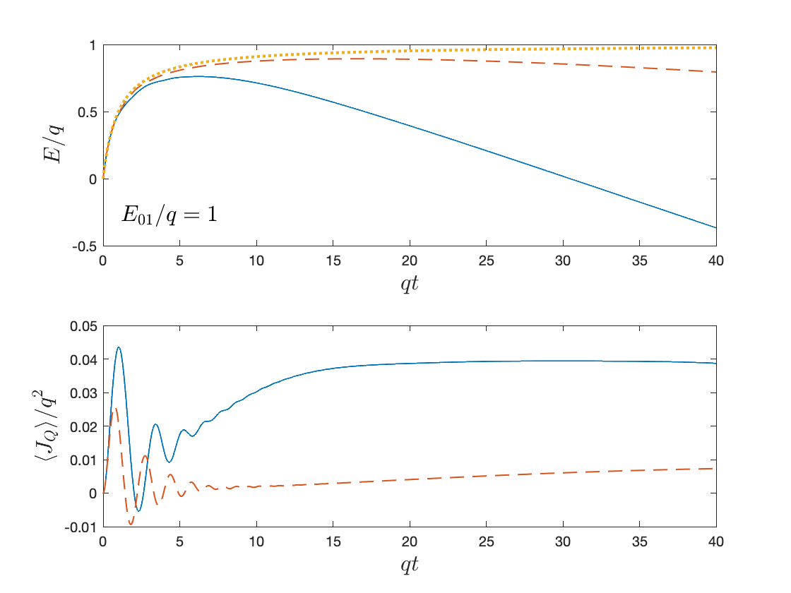
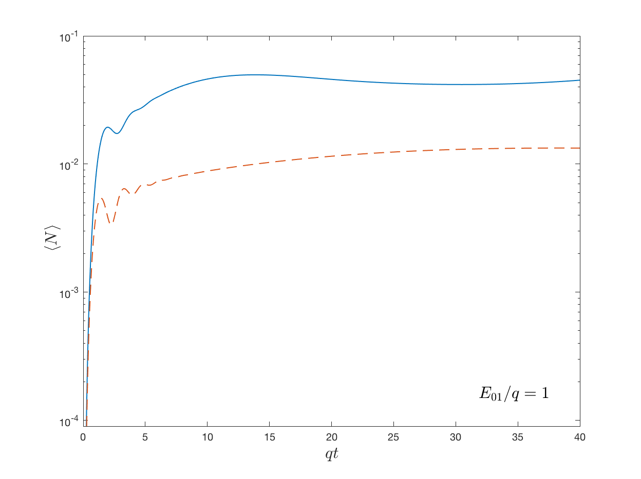
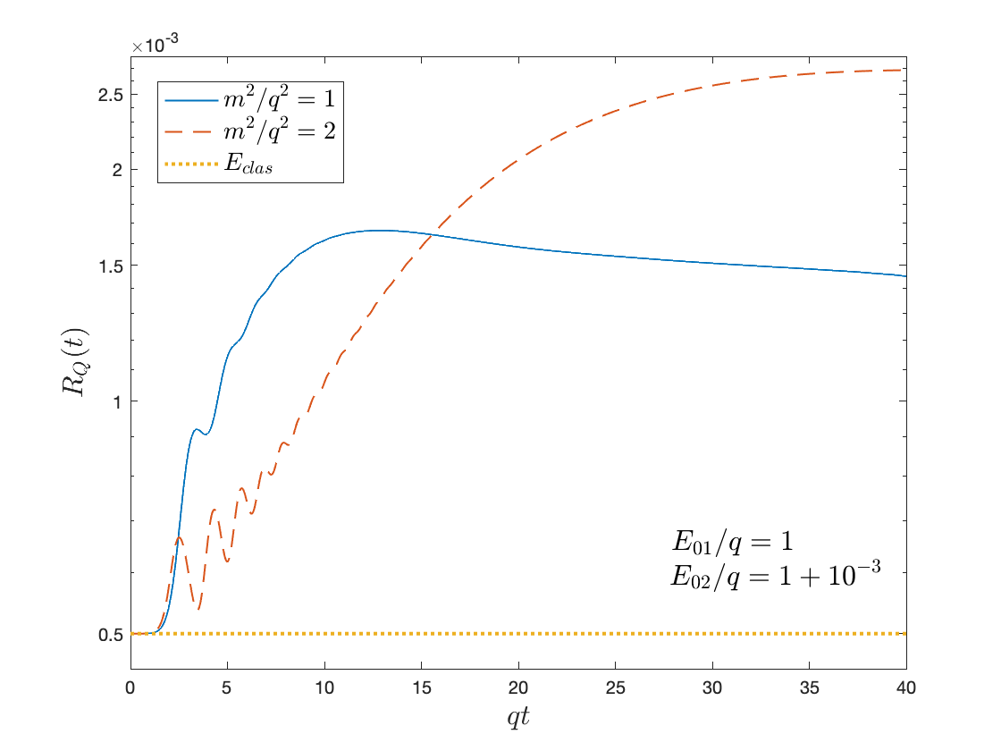
Figure 5: Results obtained from numerical solutions to the semiclassical backreaction equation for spin-$\frac{1}{2}$ fields and the asymptotically constant classical profile are shown for $E_{0}/q=1$. The masses are chosen so that $\frac{qE_{0}}{m^{2}}\leq 1$. The electric field and the induced electric current $\langle J_{Q}\rangle/q^{2}$ for each case are plotted in the left panels. Plots for the corresponding number of particles, $\langle N\rangle$, are shown in the middle panel and plots of the quantity $R_{Q}$ appear in the right panel. For the latter, the values $E_{01}/q=1$ and $E_{02}/q=1+10^{-3}$ have been chosen for the two solutions that are subtracted. The values of $m^{2}/q^{2}$ for each case are shown along with the type of curve for that solution in the legend in the right panel.

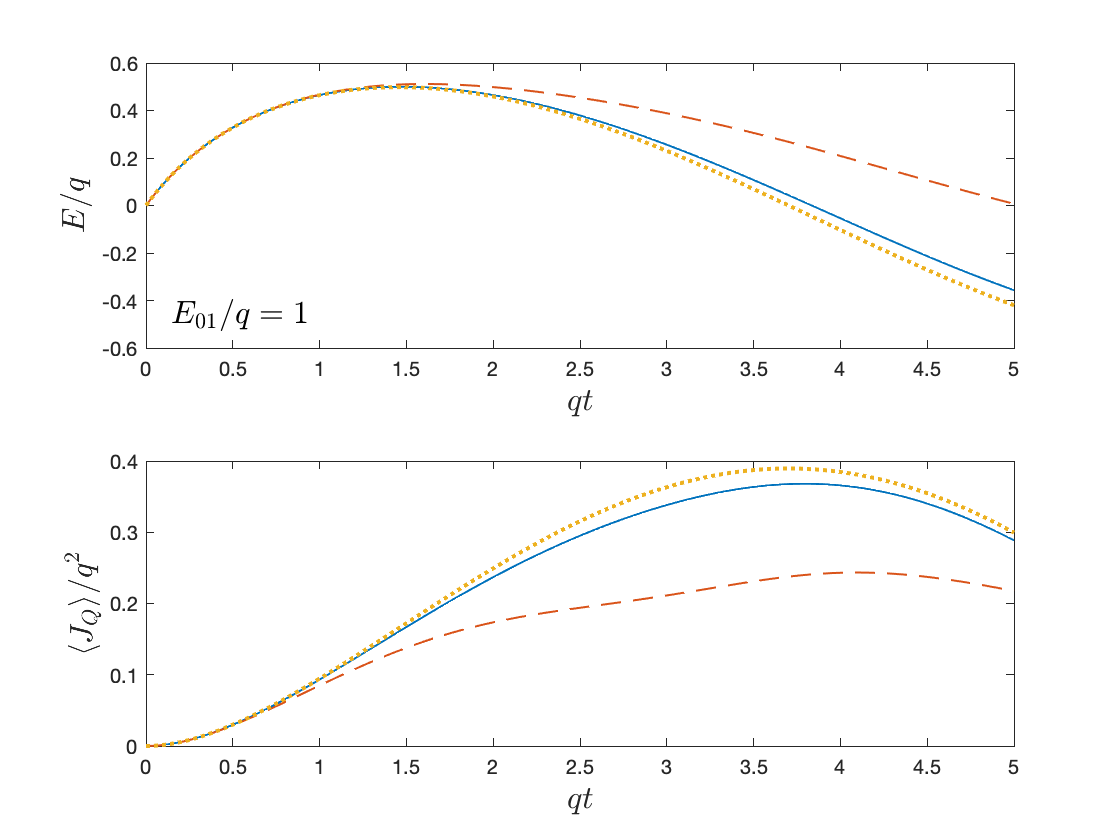
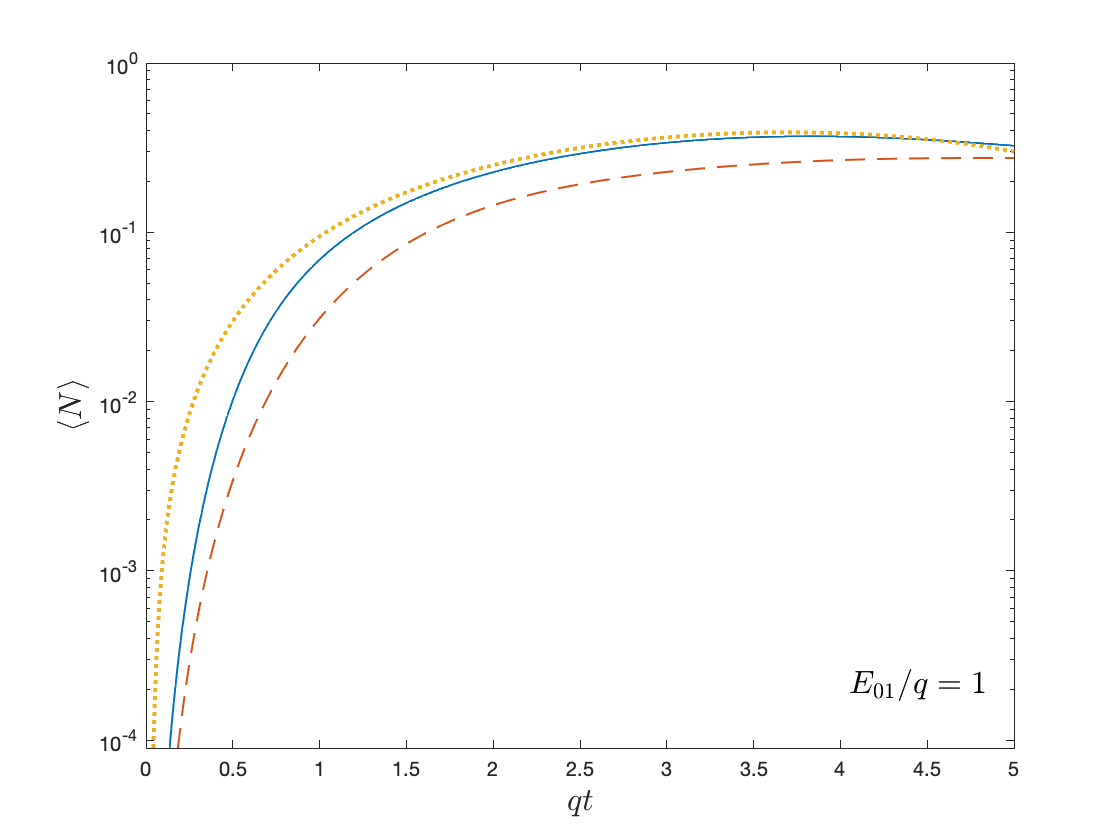
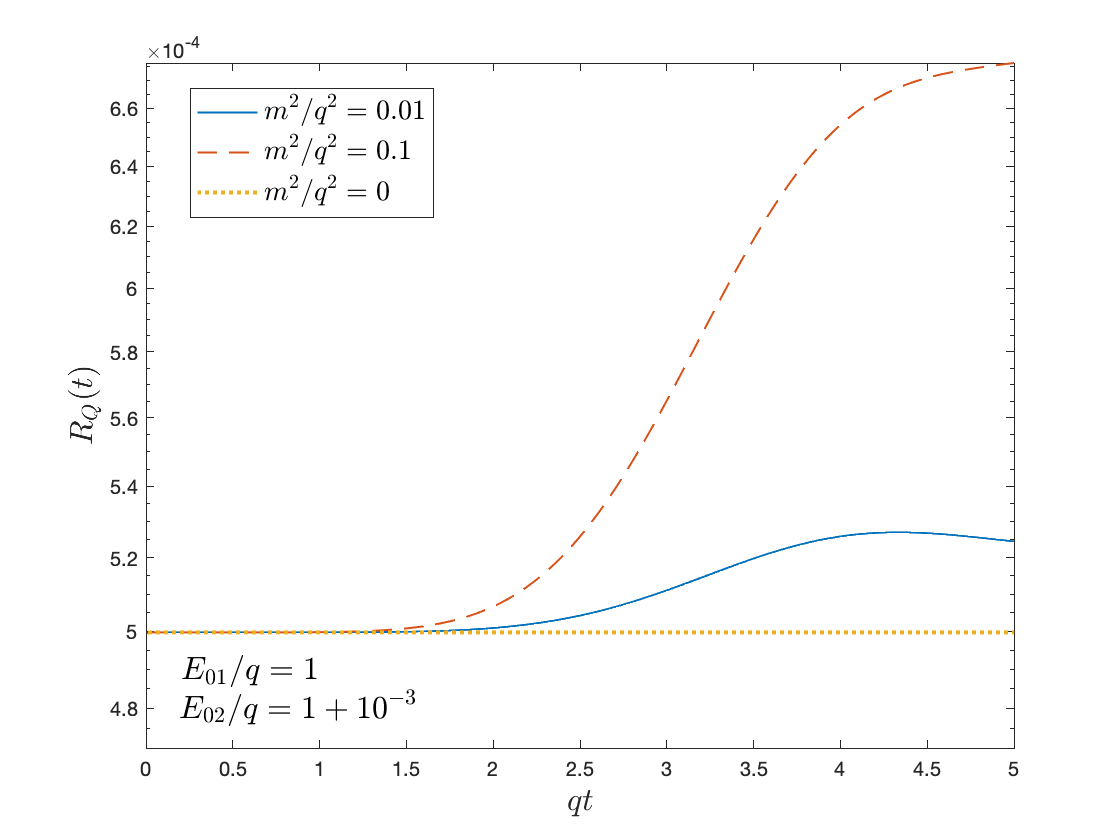
Figure 6: Results obtained from numerical solutions to the semiclassical backreaction equation for spin-$\frac{1}{2}$ fields and the asymptotically constant classical profile are shown for $E_{0}/q=1$. The masses are chosen so that $\frac{qE_{0}}{m^{2}}\geq 1$. he structure of the figure is the same as in Figure 5.

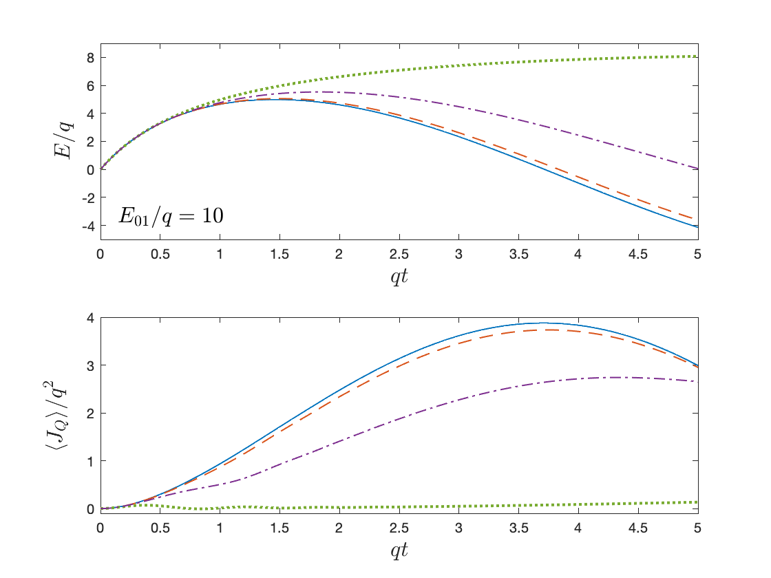
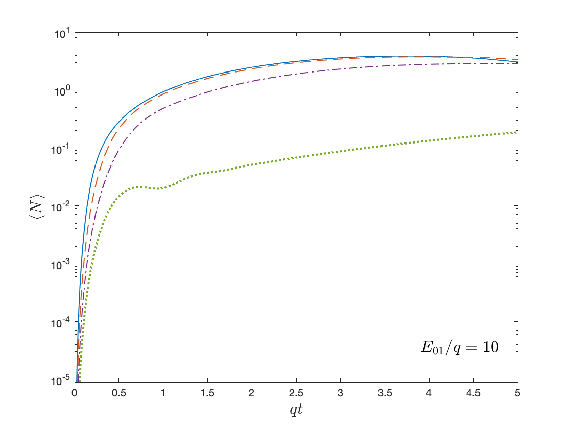
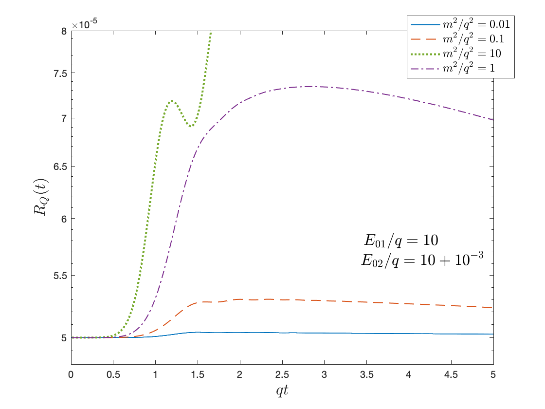
Figure 7: Results obtained from numerical solutions to the semiclassical backreaction equation for spin-$\frac{1}{2}$ fields and the asymptotically constant classical profile are shown for $E_{0}/q=10$. The masses are chosen so that $\frac{qE_{0}}{m^{2}}>1$. The structure of the figure is the same as in Figure 5. Here, the values $E_{01}/q=10$ and $E_{02}/q=10+10^{-3}$ have been chosen for the representation of the function $R_{Q}$.

V.1.3 Scalar field

Unlike the case of the spin-$\frac{1}{2}$ field, there is no clear limit that we have found as $m\to 0$ for a scalar field coupled to the electromagnetic field. However, our numerical results shown in Fig. 8 indicate that, as for the spin-$\frac{1}{2}$ field, $R_{Q}$ grows significantly at early times for $\frac{qE_{0}}{m^{2}}\sim 1$ but grows much less rapidly in time for larger values of $\frac{qE_{0}}{m^{2}}$. Thus our criterion is violated for $\frac{qE_{0}}{m^{2}}\sim 1$ but, at least for the homogeneous approximate solutions that we consider, it appears to be satisfied for $\frac{qE_{0}}{m^{2}}\gg 1$.

We have found that the behaviors of solutions to the semiclassical backreaction equation when a scalar field is present are in many ways qualitatively similar to the corresponding ones for the spin-$\frac{1}{2}$ field for cases in which the ratio $\frac{qE_{0}}{m^{2}}$ is not too large. This is illustrated in Fig. 9 for $\frac{qE_{0}}{m^{2}}=1$ and $10$. The main difference occurs for the latter case where a larger ratio results in more particle production for the scalar field than for the spin-$\frac{1}{2}$ field due to Pauli blocking. Even in that case the early-time behaviors of $R_{Q}$ are similar for the two fields.

For the large-mass limit, we expect that, as for the spin-$\frac{1}{2}$ case, the semiclassical approximation will approach the classical limit as $\frac{qE_{0}}{m^{2}}\to 0$.

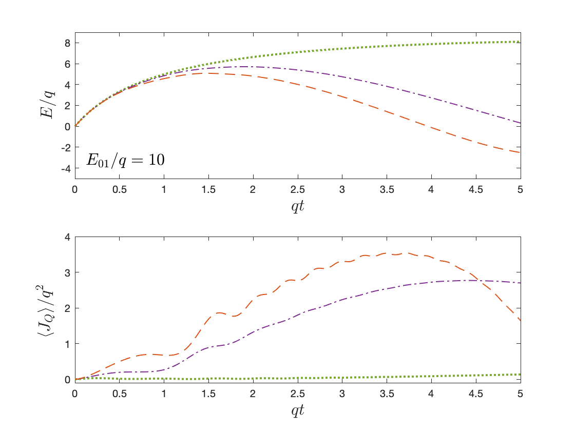
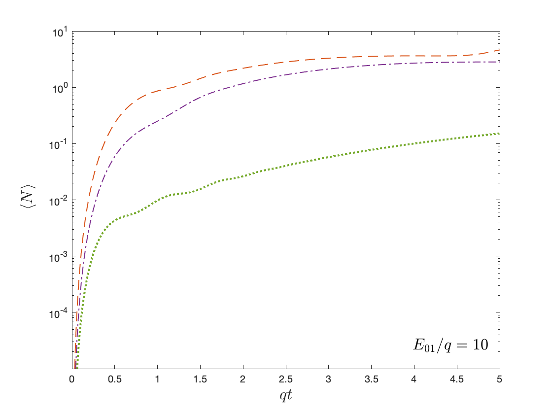
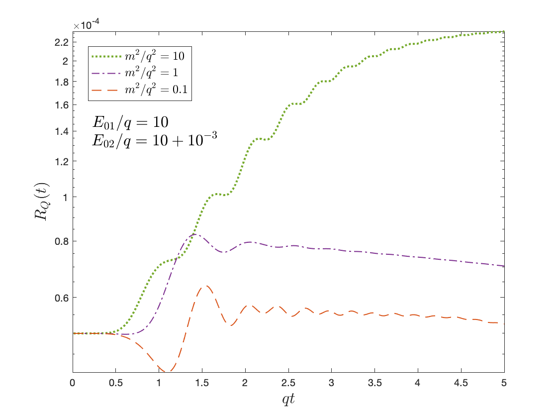
Figure 8: Results obtained from numerical solutions to the semiclassical backreaction equation for scalar fields and the asymptotically constant classical profile are shown for $E_{0}/q=10$. The masses are chosen so that $\frac{qE_{0}}{m^{2}}\geq 1$. The structure of the figure is the same as in Figure 5. We have chosen $E_{01}/q=10$ and $E_{02}/q=10+10^{-3}$ to represent the function $R_{Q}$.

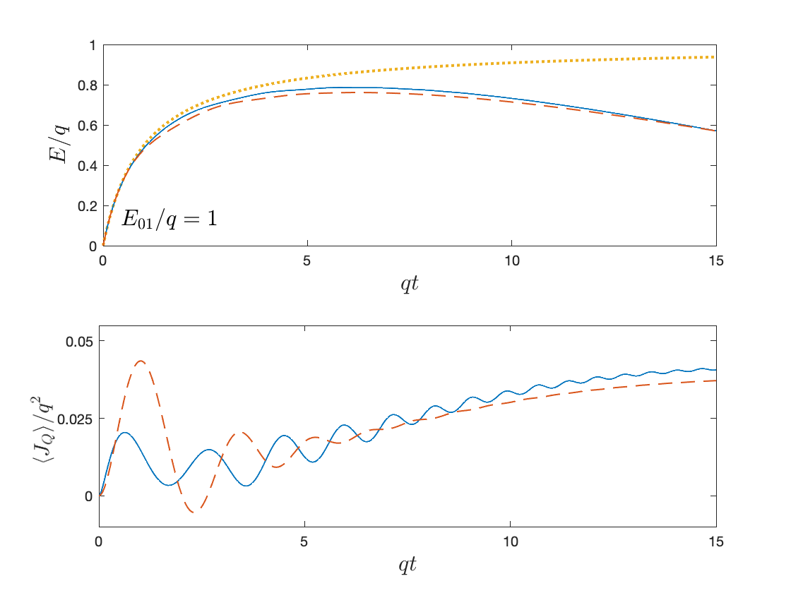
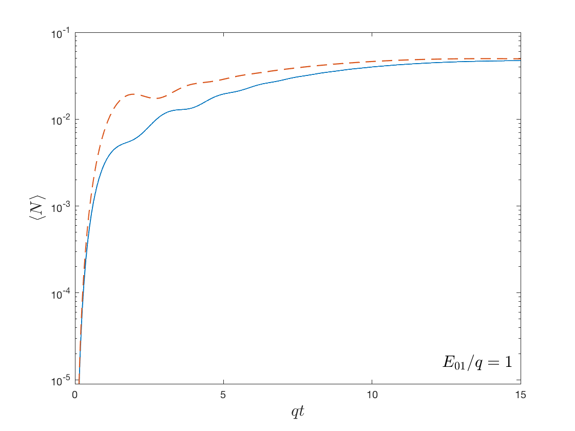
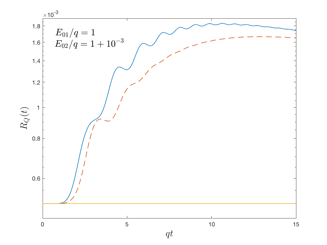
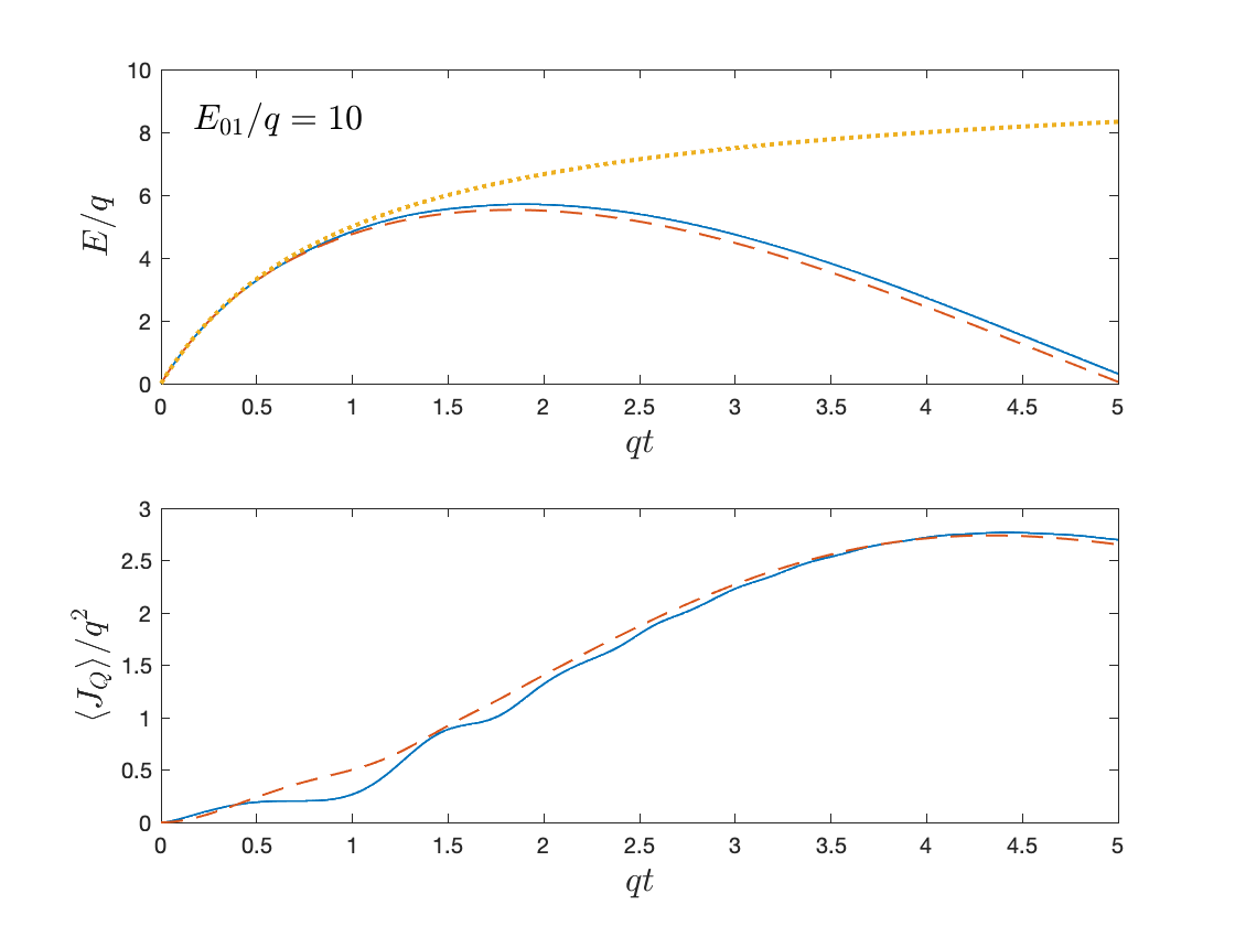
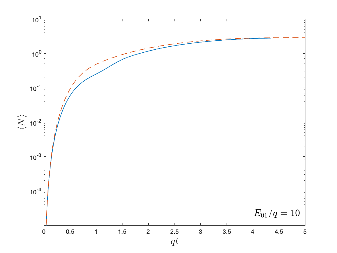
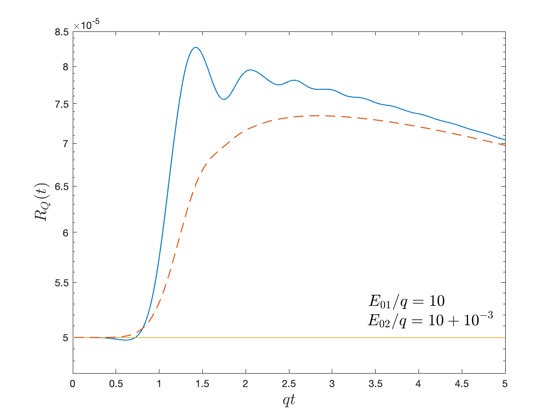
Figure 9: Results obtained from numerical solutions to the semiclassical backreaction equation for both spin-$\frac{1}{2}$ fields and scalar fields when the asymptotically constant classical profile is used are shown. For all of the plots the solid curve (blue) corresponds to the scalar field, the dashed curve (orange) corresponds to the spin-$\frac{1}{2}$ field, and the dotted curve (yellow), when shown, corresponds to the classical solution when no quantum fields are coupled to the electromagnetic field. In the upper tier $\frac{qE_{0}}{m^{2}}=1$ and $m^{2}/q^{2}=1$ while in the lower tier $\frac{qE_{0}}{m^{2}}=10$ and $m^{2}/q^{2}=1$. For each tier the left panels show plots of the electric field and the induced electric current $\langle J_{Q}\rangle/q^{2}$, the middle panel shows plots of the number of particles $\langle N\rangle$, and the right panel shows the quantity $R_{Q}$. For the latter the values $E_{01}/q=E_{0}/q$ and $E_{02}/q=E_{0}/q+10^{-3}$ have been chosen for the two solutions that are subtracted.

V.2 Sauter pulse classical profile

While our results relating to the validity of the semiclassical approximation are the same for the scalar and spin-$\frac{1}{2}$ fields for the asymptotically constant classical profile, one might be concerned that there could be significant differences for other classical profiles. To test this we have also investigated the validity of the semiclassical approximation for the Sauter pulse classical profile given in Eq. (62) with the classical current (61). Unlike the asymptotically constant classical profile, the classical current in this case is a $C^{\infty}$ function so there is no extraneous particle production due to the sudden approximation.

We find for the Sauter pulse classical profile for both the scalar and spin-$\frac{1}{2}$ cases, that $R_{Q}$ grows significantly at early times for $\frac{qE_{0}}{m^{2}}\sim 1$, as it does for the asymptotically constant classical profile, and it is bounded for $\frac{qE_{0}}{m^{2}}\gg 1$. Thus we find that our criterion for the validity of the semiclassical approximation is violated for $\frac{qE_{0}}{m^{2}}\sim 1$ while, for the approximate homogeneous solutions that we consider, our criterion appears to be satisfied for $\frac{qE_{0}}{m^{2}}\gg 1$.

Not surprisingly, given the difference between the Sauter pulse and asymptotically constant classical profiles, there are significant qualitative differences in the solutions for the electric field and in the time dependence of the number of particles that have been created. These results are illustrated in Fig. 10 for both the scalar field and spin-$\frac{1}{2}$ field cases. It is clear from the plots that for the values $\frac{qE_{0}}{m^{2}}=1$ and $10$ the backreaction effects start to be relevant before the classical pulse ends. After the effect of the classical current subsides, plasma oscillations are expected to occur because of the current created by the produced particles. There is evidence for this in the plots of the electric field. In the case $\frac{qE_{0}}{m^{2}}=1$, backreaction effects are relatively weak and the particle creation essentially ceases once the pulse in the electric field has ended. However, for $\frac{qE_{0}}{m^{2}}=10$ the initial plasma oscillation is large enough that particles are created in the scalar field case after the pulse ends.

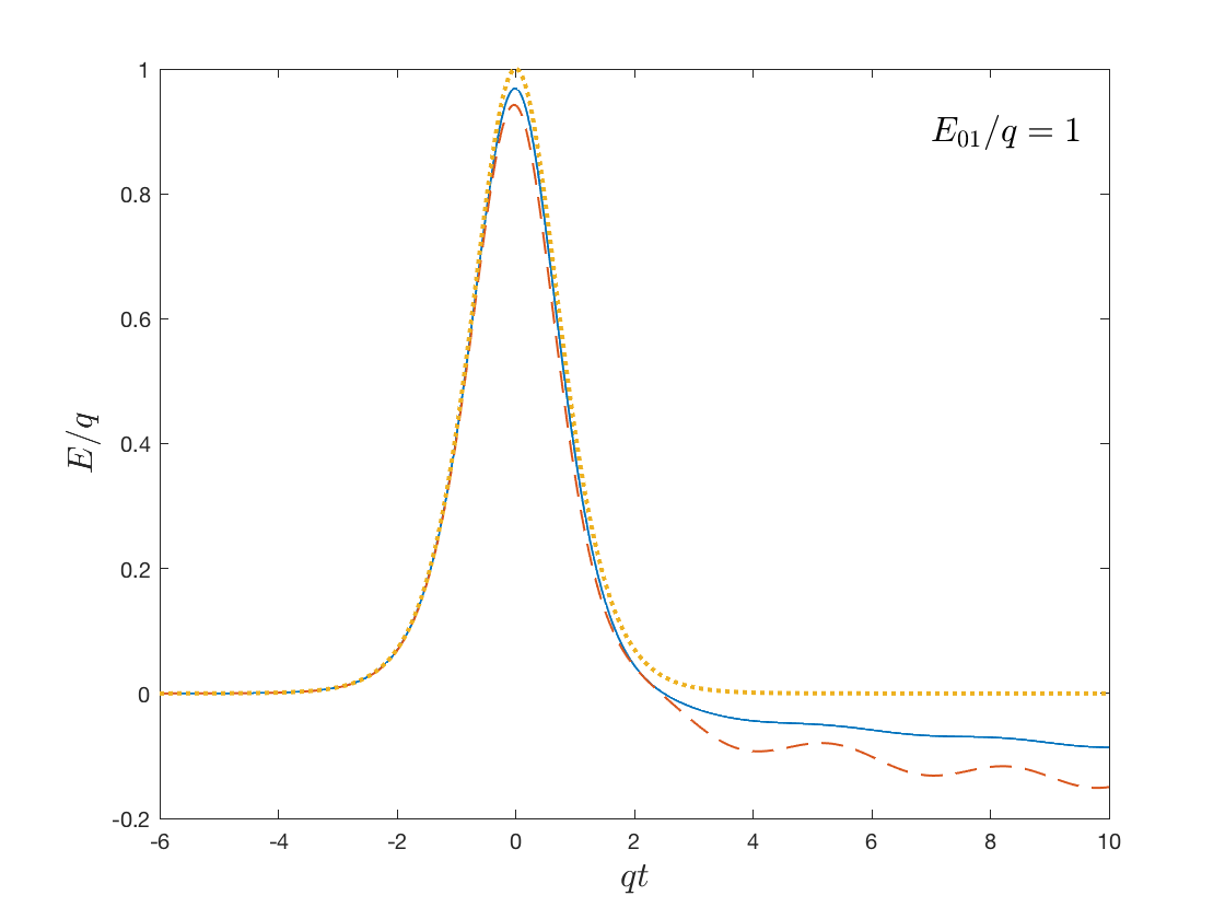
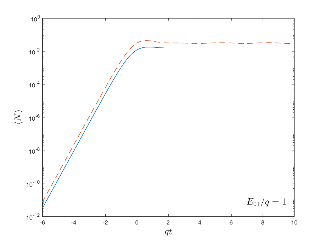
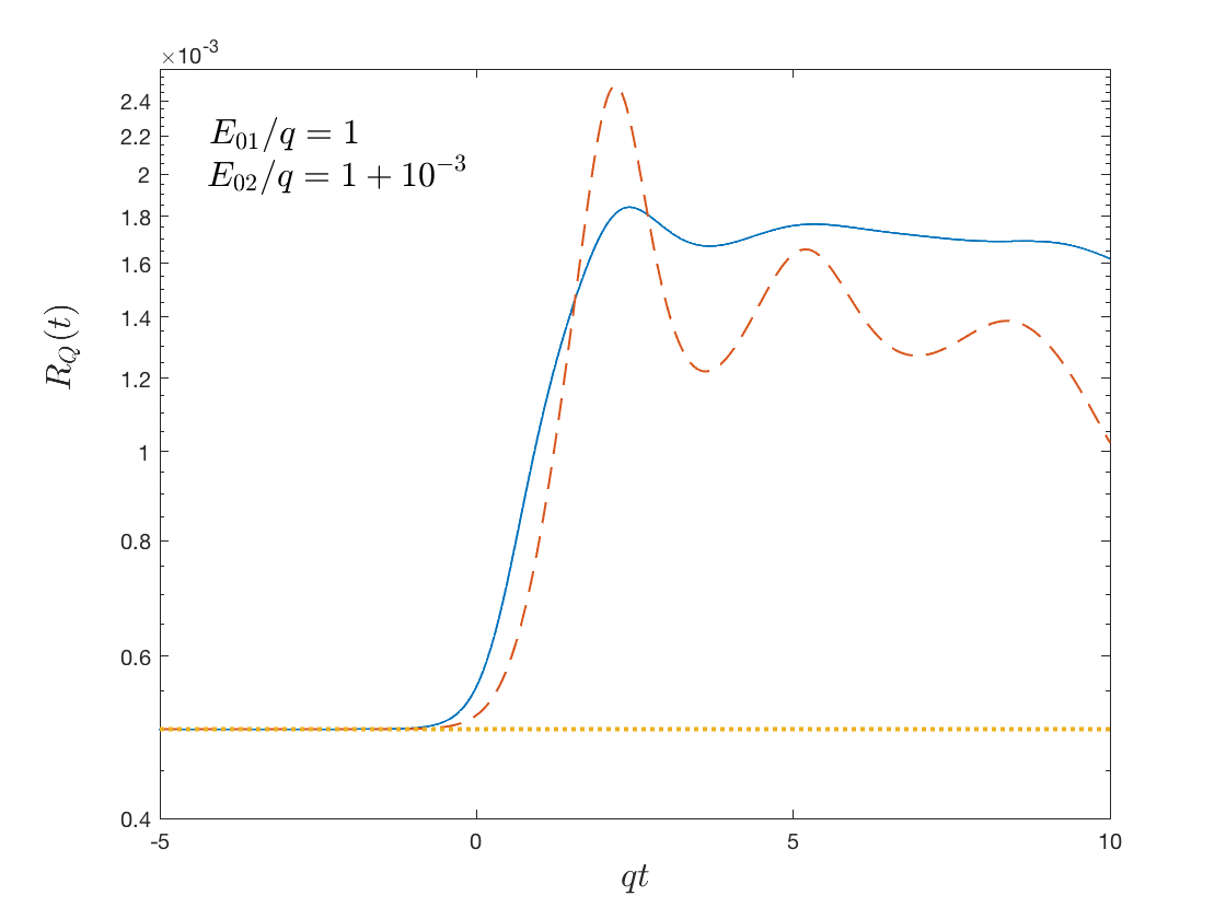
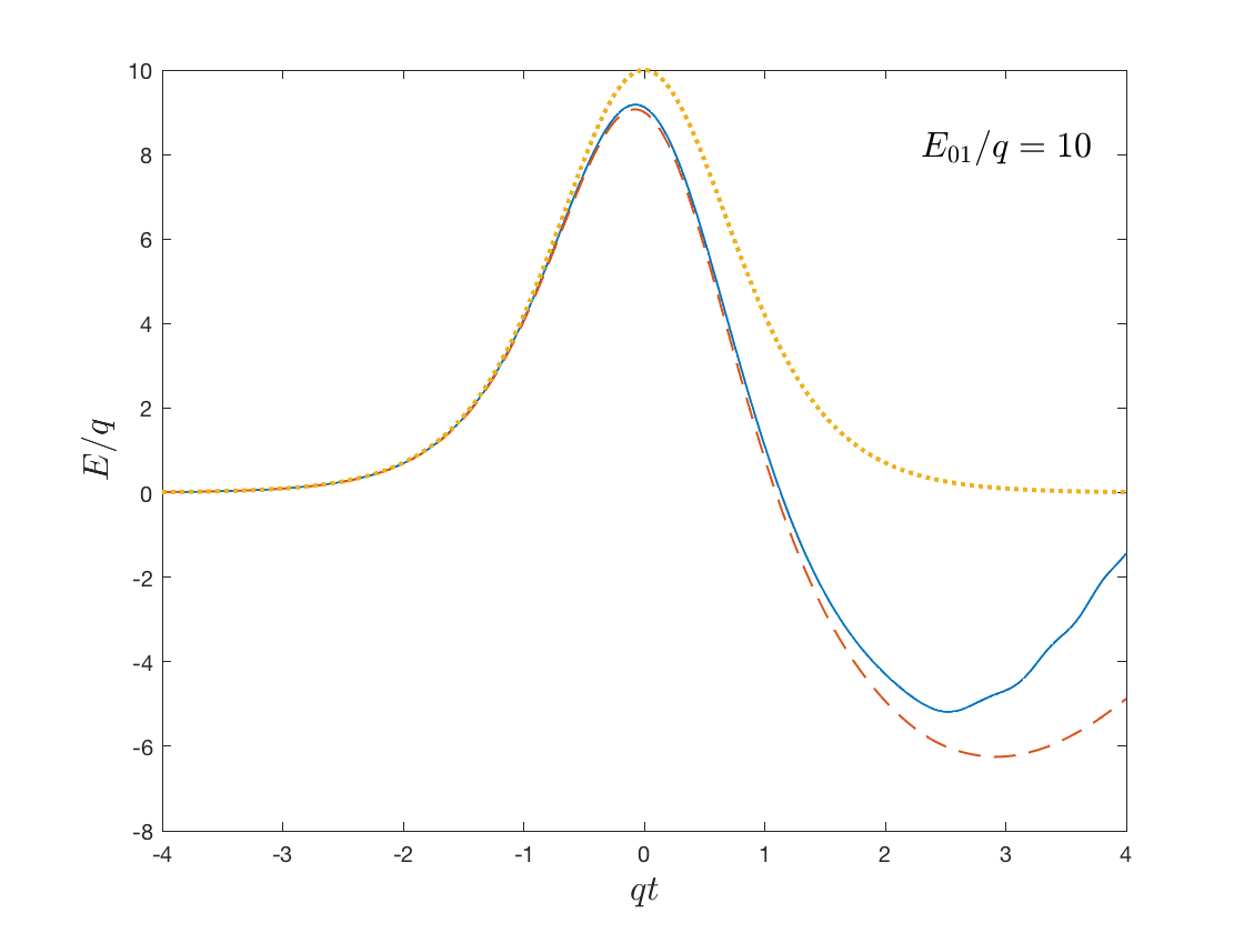
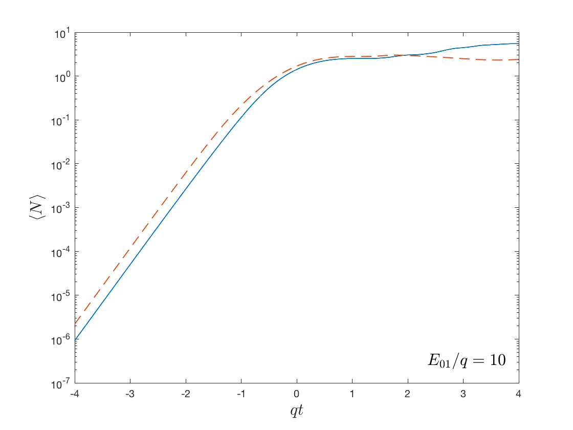
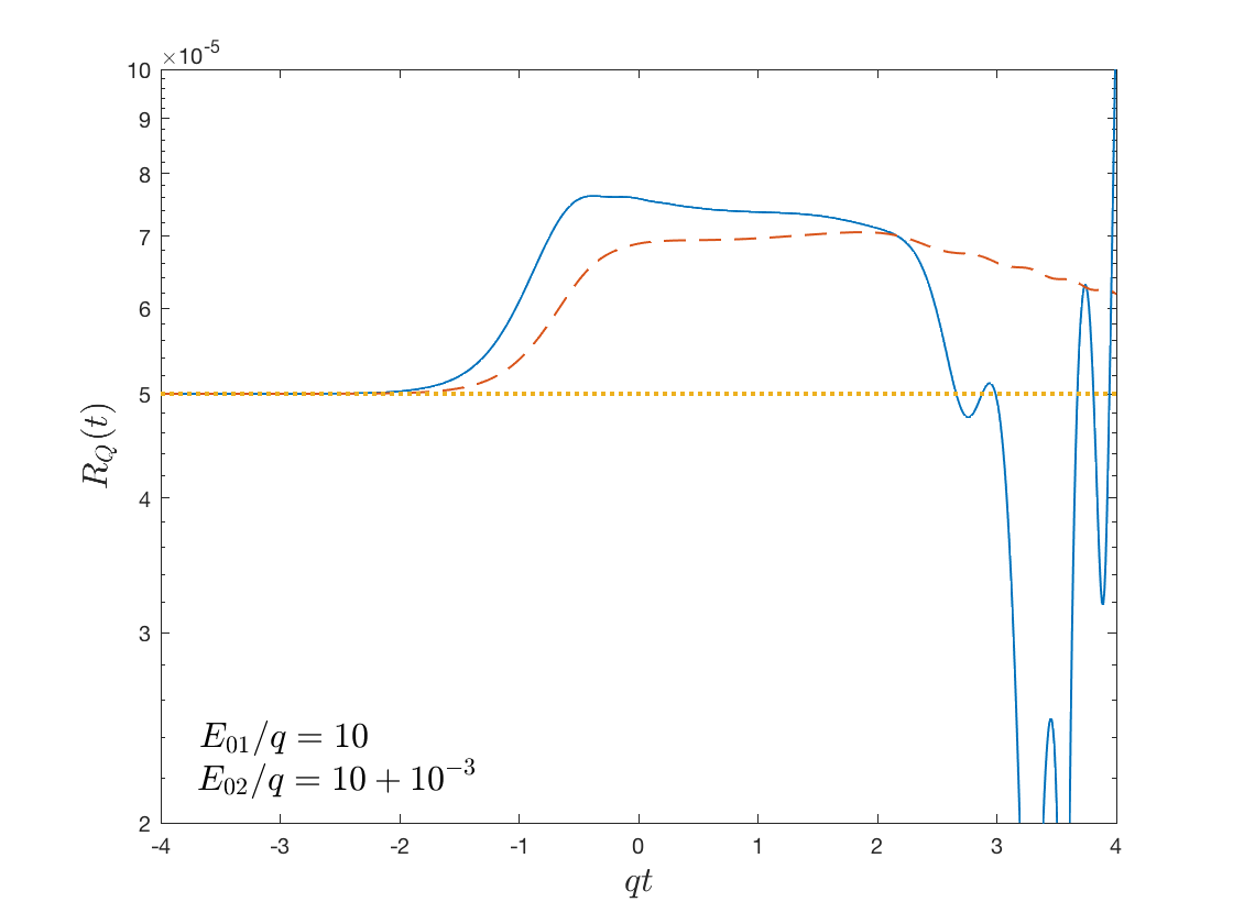
Figure 10: Results obtained from numerical solutions to the semiclassical backreaction equation for both spin-$\frac{1}{2}$ fields and scalar fields and the Sauter pulse classical profile are shown. The structure of the figure, including the initial values and the parameters of the fields, is the same than in Figure 9.

VI Conclusions and final comments

Numerical solutions to the semiclassical backreaction equation for quantum electrodynamics in 1+1D have been obtained for models of the Schwinger effect where particle production occurs due to the presence of a strong electric field. The particle production results from the coupling of either a quantized massive charged scalar field or spin-$\frac{1}{2}$ field to a classical electric field. In each case the homogeneous electric field is zero initially, as it would be in a laboratory setting, and is generated by a classical current. We have also used a renormalization scheme for the electric current and for the energy density of the quantum fields that is consistent with what would be used in a curved space background. This is different from previous backreaction calculations where the electric field was nonzero initially Kluger91 ; Kluger92 ; CMRA .

In agreement with the previous backreaction calculations, it was found that if the electric field becomes large enough so that $\frac{qE}{m^{2}}\gtrsim 1$ then a significant amount of particle production occurs. Subsequently, the produced particles create a current which generates an electric field in the opposite direction which begins to cancel the background electric field. After the initial damping of the background electric field, both the electric field and the current generated by the particles oscillate.

The particle creation process has been discussed in detail for background electric fields in Refs. and-mot-I ; dunne-part-prod ; and-mot-san . It was found that individual modes undergo a quasilocal particle creation event at roughly the time when $(k-qA)^{2}\approx m^{2}$. Here we have found that when backreaction effects are taken into account the same type of particle creation events occur. What is different is that, because of the oscillations in the the vector potential at late times, there are modes that undergo multiple particle creation events. Furthermore, once a given mode has undergone a particle creation event, it is possible for it to also undergo a particle destruction event although this does not always happen.

The total number of particles was obtained using the standard definition of a time-dependent particle number and-mot-I ; dunne-part-prod . For all three profiles considered it was found that the total particle number never decreases by any significant amount but that it is approximately constant for periods of time. This is compatible with previous calculations of the total particle number when the electric field is turned on suddenly by a classical current that is proportional to $\delta(t)$ in $3+1$D using canonical quantization Tanji and in both $1+1$D and $3+1$D using lattice simulations lattice-1 ; lattice-2 .

The energy density of the quantum field was computed for a classical current that is proportional to $\delta(t)$ and is thus zero for $t>0$. The total energy of the system is then constant and one can unambiguously track the transfer of energy between the particles and the electric field. It was found that a significant amount of energy is permanently transferred to the particles during the first damping phase of the electric field. More is then permanently transferred to the particles upon subsequent oscillations of the electric field. This is also consistent with previous calculations in $1+1$D using lattice simulations lattice-1 and in $3+1$D using canonical quantization Tanji and classical statistical field theory techniques stat-FT .

Correlations between the energy density of the particles, the current due to the particles, and the total particle number were found. In particular, times when the number of particles grows directly correspond to times when the current is changing, and times when the total number is not growing significantly correspond to times when the current is approximately constant. However, the current keeps oscillating even after the particle number stops growing significantly.

Since semiclassical electrodynamics is an approximation to quantum electrodynamics, an important question is whether this approximation is a good one for a given solution to the semiclassical backreaction equation. We have addressed this question by adapting a criterion developed for semiclassical gravity and modified for chaotic inflation models, that should be satisfied if the semiclassical approximation is valid. It is therefore a necessary but not sufficient condition. The condition is based upon the fact that the retarded two-point function for the current appears in the linear response equations for semiclassical electrodynamics. If this correlation function grows significantly in time and therefore solutions to the linear response equation grow significantly, then one expects that quantum fluctuations are significant. We have approximated homogeneous solutions to the linear response equation by taking two solutions to the semiclassical backreaction equation which are nearly the same at early times and plotting a relative difference between them which we call $R_{Q}$, defined in Eq. (58). In cases where this difference grows significantly in time one expects that the corresponding solution to the linear response equation will also do so.

We have investigated the validity of the semiclassical approximation for both the scalar and spin-$\frac{1}{2}$ fields using two different classical current profiles which are shown along with the resulting electric field (if backreaction effects are ignored) in Fig. 4.

In the zero-mass limit for the spin-$\frac{1}{2}$ field, the solutions to the semiclassical backreaction equations are completely determined by the axial anomaly. In this case, there is no growth whatsoever in the relative difference $R_{Q}$, and thus, for the approximate homogeneous solutions to the linear response equation that we considered, our criterion appears to be satisfied. We have investigated the behaviors of solutions in the small-mass case, i.e., $m^{2}\ll qE_{0}$, and found that they smoothly approach those found in the zero-mass limit. Thus, for the same type of solutions to the linear response equation, our criterion appears to be satisfied in the small-mass limit as well. Note that in this limit there is a great deal of particle production and backreaction effects are very strong (see Figs. 6 and 7). Although there is no solvable massless limit for spin-$0$ field, we have also checked numerically that there is less growth in $R_{Q}$ with time as we decrease the mass of the created particles (see Fig. 8).

The intermediate case $m^{2}\sim qE_{0}$ is very different. In both the asymptotically constant and Sauter pulse models and for both the scalar and spin-$\frac{1}{2}$ fields, once the amount of particle production has become significant, there is a rapid and significant growth in the ratio $R_{Q}$. Thus in this case our criterion is not satisfied because of this growth. This is similar to the breakdown of the semiclassical approximation found in Ref. validitypreheating for the preheating phase of chaotic inflation.

In the large-mass limit where $\frac{qE_{0}}{m^{2}}\to 0$, particle production does not occur and the behavior of the electric field can be predicted by classical electrodynamics. This is in agreement with the decoupling theorem APtheorem .

It is very likely that the first experimental verification of the Schwinger effect will be for the intermediate-mass case. Thus it is worth examining the predictions for that case more carefully. First, there is no observed growth in $R_{Q}$ at very early times before backreaction effects become significant. Therefore our criterion appears to be initially satisfied. However, given the difficulty in creating a strong enough electric field for the Schwinger effect to be observed in the laboratory (the field strength required being on the order of $E_{\rm crit}\sim 10^{18}$ V/m), the focus of the initial experiments is likely to be on the detection of particles rather than their backreaction effects. Thus the semiclassical approximation should be able to give a good description of the particle production process at such early times. Second, once backreaction effects become significant, a relatively large number of particles is likely to have been created. In previous work on the study of the validity of the semiclassical approximation for preheating in chaotic inflation validitypreheating it was found that in one case that could be compared there was good qualitative agreement with calculations that used a random-phase approximation r-p-1 ; r-p-2 ; r-p-3 even though the semiclassical approximation broke down early in the process. Similarly, the backreaction calculations in Ref. lattice-1 using classical statistical field theory techniques in 1+1 D are in qualitative agreement with our calculations of the electric field, energy density, and total particle number. Thus the semiclassical approximation can, at least in some cases, provide reasonable qualitative predictions even when its quantitative predictions cannot be trusted.

Appendix A Derivation of the linear response equation

A.1 Scalar field

The mode equation for a massive complex scalar field can be obtained by substituting Eq. (8) into Eq. (7) with the result

$$\left[-\partial_{t}^{2}+\partial_{x}^{2}-2iqA(t)\partial_{x}-q^{2}A^{2}(t)-m^{2}\right]U_{k}(t,x)=0\quad.$$ (69)

If one perturbs the vector potential about some solution to the semiclassical backreaction equation $A(t)$ such that $A(t)\to A(t)+\delta A(t)$ and writes for the mode function $U_{k}(t,x)\to U_{k}(t,x)+\delta U_{k}(t,x)$, then to leading order

$$\left[-\partial_{t}^{2}+\partial_{x}^{2}-2iqA(t)\partial_{x}-q^{2}A^{2}(t)-m^{2}\right]\delta U_{k}(t,x)=2q\delta A(t)\bigg{(}i\partial_{x}U_{k}(t,x)+qA(t)U_{k}(t,x)\bigg{)}\quad.$$ (70)

For a massive scalar field, the retarded Green’s function birrell-davies

$$G_{R}(t,x;t^{\prime},x^{\prime})=i\theta(t-t^{\prime})\langle[\phi(t,x),\phi^{\dagger}(t^{\prime},x^{\prime})]\rangle\quad,$$ (71)

is a solution to the inhomogeneous equation

$$\bigg{[}-\partial_{t}^{2}+\partial_{x}^{2}-2iqA(t)\partial_{x}-q^{2}A(t)^{2}-m^{2}\bigg{]}G_{R}(t,x;t^{\prime},x^{\prime})=-\delta(t-t^{\prime})\delta(x-x^{\prime})\quad.$$ (72)

Thus the solutions to Eq. (70) can be written in the form

$$\delta U_{k}(t,x)=\delta U_{k}^{H}(t,x)-2q\int_{-\infty}^{\infty}dt^{\prime}\int_{-\infty}^{\infty}dx^{\prime}G_{R}(t,x;t^{\prime},x^{\prime})\left[i\,\partial_{x^{\prime}}+q\,A(t^{\prime})\right]U_{k}(t^{\prime},x^{\prime})\delta A(t^{\prime})\quad,$$ (73)

where $\delta U_{k}^{H}(t,x)$ is a solution to the homogeneous part of Eq. (70).

The explicit form of $G_{R}(x,x^{{}^{\prime}})$ can be found using Eq. (71) with Eq. (11) evaluated in the vacuum state, which yields

$$G_{R}(t,x;t^{\prime}x^{\prime})=\frac{i}{2\pi}\theta(t-t^{{}^{\prime}})\int_{-\infty}^{\infty}dk\bigg{[}f_{k}(t)f_{k}^{*}(t^{{}^{\prime}})-f_{k}(t^{{}^{\prime}})f_{k}^{*}(t)\bigg{]}e^{ik(x-x^{{}^{\prime}})}\quad.$$ (74)

Restricting attention to spatially homogeneous perturbations we have

$$\delta U_{k}(t,x)=\delta f_{k}(t)e^{ikx}\;.$$ (75)

Substituting Eqs. (74) and (75) into Eq. (73) and integrating yields

$$\delta f_{k}(t)=\delta f_{k}^{H}(t)+2\,i\,q\int_{-\infty}^{t}dt^{\prime}\bigg{(}k-qA(t^{\prime})\bigg{)}\bigg{[}f_{k}(t)f_{k}^{*}(t^{\prime})-f_{k}(t^{\prime})f_{k}^{*}(t)\bigg{]}f_{k}(t^{\prime})\delta A(t^{\prime})\quad.$$ (76)

The perturbation of the renormalized current (23) yields

$$\delta\langle J_{Q}\rangle_{\rm ren}=\frac{q}{\pi}\int_{-\infty}^{\infty}dk\,\bigg{[}\bigg{(}k-qA(t)\bigg{)}\bigg{[}f_{k}(t)\delta f_{k}^{*}(t)+\delta f_{k}(t)f_{k}^{*}(t)\bigg{]}-q|f_{k}(t)|^{2}\delta A(t)+\frac{q\,m^{2}}{2\omega^{3}}\delta A(t)\bigg{]}\quad.$$ (77)

Substituting Eq. (76) and its complex conjugate into Eq. (77) yields

$$\delta\langle J_{Q}\rangle_{\rm ren} = \frac{q}{\pi}\int_{-\infty}^{\infty}dk\,\left\{\bigg{(}k-qA(t)\bigg{)}\bigg{[}f_{k}(t)\delta f_{k}^{*H}(t)+f_{k}^{*}(t)\delta f_{k}^{H}(t)\bigg{]}-\bigg{[}|f_{k}(t)|^{2}-\frac{m^{2}}{2\omega^{3}}\bigg{]}q\,\delta A(t)\right\}$$ (78)

$$\qquad-\frac{4q^{2}}{\pi}\int_{-\infty}^{\infty}dk\int_{-\infty}^{t}dt^{\prime}\bigg{(}k-qA(t)\bigg{)}\bigg{(}k-qA(t^{\prime})\bigg{)}\textnormal{Im}\bigg{\{}f_{k}(t)^{2}f_{k}^{*}(t^{\prime})^{2}\bigg{\}}\delta A(t^{\prime})\quad.$$

Our goal is to show that the above linear response equation can be written in terms of the two-point correlation function for the current, $\langle[J_{Q}(t,x),J_{Q}(t^{\prime},x^{\prime})]\rangle$. To accomplish this we next calculate the two-point correlation function using the symmetrized current density (20) and the scalar field mode expansion (11) evaluated in the vacuum state. After integrating over the spatial coordinate one finds

$$\int_{-\infty}^{\infty}dx^{\prime}\langle[J_{Q}(t,x),J_{Q}(t^{\prime},x^{\prime})]\rangle=\frac{4\,i\,q^{2}}{\pi}\int_{-\infty}^{\infty}dk\bigg{(}k-qA(t)\bigg{)}\bigg{(}k-qA(t^{\prime})\bigg{)}\textnormal{Im}\bigg{\{}f_{k}(t)^{2}f_{k}^{*}(t^{\prime})^{2}\bigg{\}}\quad.$$ (79)

Comparing Eqs. (78) and (79), it is clear that Eq. (78) can be written in the form

$$\delta\langle J_{Q}\rangle_{\rm ren} = \frac{q}{\pi}\int_{-\infty}^{\infty}dk\,\bigg{[}\bigg{(}k-qA(t)\bigg{)}\bigg{[}f_{k}(t)\delta f_{k}^{*H}(t)+f_{k}^{*}(t)\delta f_{k}^{H}(t)\bigg{]}-\bigg{[}|f_{k}(t)|^{2}-\frac{m^{2}}{2\omega^{3}}\bigg{]}q\,\delta A(t)\bigg{]}$$ (80)

$$\qquad\qquad\qquad\qquad\qquad\qquad+\,i\int_{-\infty}^{\infty}dx^{\prime}\int_{-\infty}^{t}dt^{\prime}\,\langle[J_{Q}(t,x),J_{Q}(t^{\prime},x^{\prime})]\rangle\delta A(t^{\prime})\quad.$$

Thus $\delta\langle J_{Q}\rangle_{\rm ren}$ for a scalar field has been cast in terms of the current-current two-point correlation function. Note that $\delta f_{k}^{H}(t)$ corresponds to a change of state of the quantum field. For the cases considered in this paper the vector potential and its first time derivative are zero initially so the perturbations do not cause a change in the state of the field so $\delta f_{k}^{H}(t)=0$. Then the linear response equation (47) becomes

$$\frac{d^{2}}{dt^{2}}\delta A(t) = -\frac{d}{dt}\delta E(t)=\delta J_{C}-\frac{q^{2}}{\pi}\delta A(t)\int_{-\infty}^{\infty}dk\,\left[|f_{k}(t)|^{2}-\frac{m^{2}}{2\omega^{3}}\right]$$

$$\qquad\qquad\qquad\qquad\qquad\qquad\qquad\qquad\qquad+\,i\int_{-\infty}^{\infty}dx^{\prime}\int_{-\infty}^{t}dt^{\prime}\,\langle[J_{Q}(t,x),J_{Q}(t^{\prime},x^{\prime})]\rangle\delta A(t^{\prime})\quad.$$

A.2 Spin-$\frac{1}{2}$ field

The mode equation for a massive charged spin $\frac{1}{2}$ field can be obtained by substituting Eq. (15) into Eq. (14) with the result

$$\bigg{[}i\,\gamma^{t}\partial_{t}+i\,\gamma^{x}\partial_{x}+q\,\gamma^{x}A(t)-m\bigg{]}u_{k}(t,x)=0\quad.$$ (82)

If one perturbs the vector potential about some solution to the semiclassical backreaction equation $A(t)$ such that $A(t)\to A(t)+\delta A(t)$ and writes for the mode function $u_{k}(t,x)\to u_{k}(t,x)+\delta u_{k}(t,x)$ then to leading order

$$\bigg{[}i\,\gamma^{t}\partial_{t}+i\,\gamma^{x}\partial_{x}+q\,\gamma^{x}A(t)-m\bigg{]}\delta u_{k}(t,x)=-q\gamma^{x}u_{k}(t,x)\delta A(t)\quad.$$ (83)

For a massive spin-$\frac{1}{2}$ field the retarded Green’s function

$$G_{R}(t,x;t^{\prime},x^{\prime})=i\,\theta(t-t^{\prime})\langle\{\psi(t,x),\bar{\psi}(t^{\prime},x^{\prime})\}\rangle\quad,$$ (84)

is a solution to the inhomogeneous equation

$$\bigg{[}i\,\gamma^{t}\partial_{t}+i\,\gamma^{x}\partial_{x}+q\,\gamma^{x}A(t)-m\bigg{]}G_{R}(t,x;t^{\prime},x^{\prime})=-\mathbbm{1}\,\delta(t-t^{\prime})\delta(x-x^{\prime})\quad,$$ (85)

where $\mathbbm{1}$ is the identity matrix. Thus the solution to Eq. (83) can be written in the form

$$\delta u_{k}(t,x)=\delta u_{k}^{H}(t,x)+q\int_{-\infty}^{\infty}dt^{\prime}\int_{-\infty}^{\infty}dx^{\prime}\,G_{R}(t,x;t^{\prime},x^{\prime})\,\gamma^{x}\,\delta A(t^{{}^{\prime}})\,u_{k}(t^{\prime},x^{\prime})\quad.$$ (86)

where $H$ represents the homogeneous solution. The explicit form of $G_{R}(x,x^{{}^{\prime}})$ can be found using Eq. (84) with the Dirac field expansion (15) in terms of spinor solutions (16) evaluated in the vacuum state, which yields

$$G_{R}(t,x;t^{\prime},x^{\prime})=\frac{i\,\theta(t-t^{{}^{\prime}})}{2\pi}\int dk\,e^{ik(x-x^{{}^{\prime}})}\begin{bmatrix}-h_{k}^{I}(t)h_{k}^{II*}(t^{{}^{\prime}})+h_{k}^{II*}(t)h_{k}^{I}(t^{{}^{\prime}})&h_{k}^{I}(t)h_{k}^{I*}(t^{{}^{\prime}})+h_{k}^{II*}(t)h_{k}^{II}(t^{{}^{\prime}})\\ \\ h_{k}^{II}(t)h_{k}^{II*}(t^{{}^{\prime}})+h_{k}^{I*}(t)h_{k}^{I}(t^{{}^{\prime}})&-h_{k}^{II}(t)h_{k}^{I*}(t^{{}^{\prime}})+h_{k}^{I*}(t)h_{k}^{II}(t^{{}^{\prime}})\end{bmatrix}\quad.$$ (87)

Restricting attention to spatially homogeneous perturbations and using Eq. (16) gives

$$\delta u_{k}(t,x)=\frac{e^{ikx}}{\sqrt{2\pi}}\begin{bmatrix}\delta h_{k}^{I}(t)\\ -\delta h_{k}^{II}(t)\end{bmatrix}\quad.$$ (88)

Changing the integration variable to $k^{\prime}$ in (87), substituting the result along with (82) and (88) into (86), and integrating first over $x^{\prime}$ and then over $k^{\prime}$ gives

$$\begin{bmatrix}\delta h_{k}^{I}(t)\\ \\ -\delta h_{k}^{II}(t)\end{bmatrix} = \begin{bmatrix}\delta h_{k}^{IH}(t)\\ \\ -\delta h_{k}^{IIH}(t)\end{bmatrix}-i\,q\int_{-\infty}^{t}dt^{{}^{\prime}}\begin{bmatrix}h_{k}^{I}(t)\bigg{(}|h_{k}^{I}(t^{{}^{\prime}})|^{2}-|h_{k}^{II}(t^{{}^{\prime}})|^{2}\bigg{)}+2h_{k}^{II*}(t)h_{k}^{I}(t^{{}^{\prime}})h_{k}^{II}(t^{{}^{\prime}})\\ \\ h_{k}^{II}(t)\bigg{(}|h_{k}^{II}(t^{{}^{\prime}})|^{2}-|h_{k}^{I}(t^{{}^{\prime}})|^{2}\bigg{)}+2h_{k}^{I*}(t)h_{k}^{I}(t^{{}^{\prime}})h_{k}^{II}(t^{{}^{\prime}})\end{bmatrix}\delta A(t^{{}^{\prime}})\quad.$$

The perturbation of the renormalized current (26) yields

$$\delta\langle J_{Q}\rangle_{\textnormal{ren}}=\frac{q}{2\pi}\int_{-\infty}^{\infty}dk\,\bigg{[}h_{k}^{I*}(t)\delta h_{k}^{I}(t)+h_{k}^{I}(t)\delta h_{k}^{I*}(t)-h_{k}^{II*}(t)\delta h_{k}^{II}(t)-h_{k}^{II}(t)\delta h_{k}^{II*}(t)-\frac{q\,m^{2}}{\omega^{3}}\delta A(t)\bigg{]}\quad.$$ (90)

Equation (A.2) and its complex conjugate can be substituted into Eq. (90) to yield

$$\delta\langle J_{Q}\rangle_{\rm ren} = \frac{q}{2\pi}\int_{-\infty}^{\infty}dk\,\bigg{[}h_{k}^{I*}(t)\,\delta h_{k}^{I,H}(t)+h_{k}^{I}(t)\,\delta h_{k}^{I*H}(t)-h_{k}^{II*}(t)\,\delta h_{k}^{II,H}(t)-h_{k}^{II}(t)\,\delta h_{k}^{II*H}(t)-\frac{q\,m^{2}}{\omega^{3}}\delta A(t)\bigg{]}$$

$$\qquad\qquad\qquad\qquad\qquad\qquad-\frac{4\,q^{2}}{\pi}\int_{-\infty}^{\infty}dk\int_{-\infty}^{t}dt^{{}^{\prime}}\textnormal{Im}\bigg{\{}h^{I}(t)h^{II}(t)h^{I*}(t^{{}^{\prime}})h^{II*}(t^{{}^{\prime}})\bigg{\}}\delta A(t^{{}^{\prime}})\quad.$$

As in the scalar field case, an explicit expression for the two-point correlation function is needed. To calculate the two-point correlation function we begin by utilizing the antisymmetrized current density (25) with the fermion field mode expansion (15) evaluated in the vacuum state. Integrating over the spatial coordinate gives

$$\int_{-\infty}^{\infty}dx^{{}^{\prime}}\langle[J_{Q}(t,x),J_{Q}(t^{\prime},x^{\prime})]\rangle=\frac{4i\,q^{2}}{\pi}\int_{-\infty}^{\infty}dk\,\textnormal{Im}\bigg{\{}h_{k}^{I}(t)h_{k}^{II}(t)h_{k}^{I*}(t^{{}^{\prime}})h_{k}^{II*}(t^{{}^{\prime}})\bigg{\}}\quad.$$ (92)

Comparing Eqs. (LABEL:deltaJdirac) and (92), it is clear that Eq. (LABEL:deltaJdirac) can be written in the form

$$\delta\langle J_{Q}\rangle_{\textnormal{ren}} = \frac{q}{2\pi}\int_{-\infty}^{\infty}dk\,\bigg{[}h_{k}^{I*}(t)\,\delta h_{k}^{I,H}(t)+h_{k}^{I}(t)\,\delta h_{k}^{I*H}(t)-h_{k}^{II*}(t)\,\delta h_{k}^{II,H}(t)-h_{k}^{II}(t)\,\delta h_{k}^{II*H}(t)$$ (93)

$$\qquad\qquad\qquad-\frac{q\,m^{2}}{\omega^{3}}\delta A(t)\bigg{]}+\,i\int_{-\infty}^{\infty}dx^{{}^{\prime}}\int_{-\infty}^{t}dt^{{}^{\prime}}\langle[J_{Q}(t,x),J_{Q}(t^{\prime},x^{\prime})]\rangle\,\delta A(t^{{}^{\prime}})\quad.$$

Thus $\delta\langle J_{Q}\rangle_{\textnormal{ren}}$ for spin-$\frac{1}{2}$ particle production has been cast in terms of the current-current two-point correlation function. Note that $\delta h_{k}^{(I,II)H}(t)$ corresponds to a change of state of the quantum field. As mentioned above, for the cases considered in this paper the vector potential and its first time derivative are zero initially so the perturbations do not cause a change in the state of the field so $\delta h_{k}^{(I,II)H}(t)=0$. Then the linear response equation (47) becomes

$$\frac{d^{2}}{dt^{2}}\delta A(t)=-\frac{d}{dt}\delta E(t)=\delta J_{C}-\frac{q^{2}m^{2}}{2\pi}\delta A(t)\int_{-\infty}^{\infty}\frac{dk}{\omega^{3}}+i\int_{-\infty}^{\infty}dx^{{}^{\prime}}\int_{-\infty}^{t}dt^{{}^{\prime}}\langle[J_{Q}(t,x),J_{Q}(t^{\prime},x^{\prime})]\rangle\,\delta A(t^{{}^{\prime}})\quad.$$ (94)

References

- (1) J. Schwinger, Phys. Rev. 82, 664 (1951).
- (2) L. Parker, The creation of particles in an expanding universe, Ph.D. thesis, Harvard University, 1966; Dissexpress.umi.com, Publication No. 7331244; Phys. Rev. Lett. 21, 562 (1968); Phys. Rev. 183, 1057 (1969); Phys. Rev. D 3, 346 (1971).
- (3) S.W. Hawking, Commun. Math. Phys. 43, 199 (1975).
- (4) L. Parker and D. J. Toms, Quantum Field Theory in Curved Spacetime: Quantized Fields and Gravity (Cambridge University Press, Cambridge, England, 2009).
- (5) N. D. Birrell and P. C. W. Davies, Quantum Fields in Curved Space (Cambridge University Press, Cambridge, England, 1982).
- (6) M. D. Schwartz, Quantum Field Theory and the Standard Model (Cambridge University Press, Cambridge, England, 2014).
- (7) Y. Kluger, J. M. Eisenberg, B. Svetitsky, F. Cooper and E. Mottola, Phys. Rev. Lett. 67, 2427 (1991).
- (8) Y. Kluger, J. M. Eisenberg, B. Svetitsky, F. Cooper and E. Mottola, Phys. Rev. D 45, 4659 (1992).
- (9) Y. Kluger, J. M. Eisenberg, and B. Svetitsky, Int. J. Mod.Phys. E 02, 333 (1993).
- (10) N. Tanji, Ann. Phys. (Amsterdam) 324, 1691 (2009).
- (11) F. Gelis and N. Tanji, Phys. Rev. D 87, 125035 (2013).
- (12) J. C. R. Bloch, V. A. Mizerny, A. V. Prozorkevich, C. D. Roberts, S. M. Schmidt, S. A. Smolyansky, and D. V. Vinnik, Phys. Rev. D 60, 116011 (1999).
- (13) F. Hebenstreit, J. Berges, and D. Gelfand, Phys. Rev. D 87, 105006 (2013).
- (14) V. Kasper, F. Hebenstreit, and J. Berges, Phys. Rev. D 90, 025016 (2014).
- (15) F. Sauter, Z. Phys. 69, 742 (1931).
- (16) P. R. Anderson and E. Mottola, Phys. Rev. D 89, 104038 (2014).
- (17) R. Dabrowski and G. V. Dunne, Phys. Rev. D 90, 025021 (2014).
- (18) P. R. Anderson, E. Mottola, and D. H. Sanders, Phys. Rev. D 97, 065016 (2018).
- (19) J. Schwinger, Phys. Rev. 128, 2425 (1962).
- (20) P. R. Anderson, C. Molina-Paris, and D. H. Sanders, Phys. Rev. D 92, 083522 (2015).
- (21) P. R. Anderson, C. Molina-Paris, and E. Mottola, Phys. Rev. D 67, 024026 (2003).
- (22) P. R. Anderson, C. Molina-Paris, and E. Mottola, Phys. Rev. D 80, 084005 (2009).
- (23) A. Ferreiro and J. Navarro-Salas, Phys. Rev. D 97, 125012 (2018).
- (24) P. Beltrán-Palau, J. Navarro-Salas, and S. Pla, Phys. Rev. D 99, 105008 (2019).
- (25) L. Parker and S. A. Fulling, Phys. Rev. D 9, 341 (1974); S. A. Fulling and L. Parker, Ann. Phys. (N.Y.) 87, 176 (1974).
- (26) N. D. Birrell, Proc. R. Soc. B 361, 513 (1978).
- (27) P. R. Anderson and L. Parker, Phys. Rev. D 36, 2963 (1987).
- (28) A. Landete, J. Navarro-Salas, and F. Torrenti, Phys. Rev. D 88, 061501 (2013).
- (29) A. Landete, J. Navarro-Salas, and F. Torrenti, Phys. Rev. D 89, 044030 (2014).
- (30) A. del Rio, J. Navarro-Salas, and F. Torrenti, Phys. Rev. D 90, 084017 (2014).
- (31) S. Ghosh, Phys. Rev. D 91, 124075 (2015).
- (32) S. Ghosh, Phys. Rev. D 93, 044032 (2016).
- (33) J. F. Barbero G., A. Ferreiro, J. Navarro-Salas, and E. J. S. Villaseñor, Phys. Rev. D 98, 025016 (2018).
- (34) F. Cooper, E. Mottola, B. Rogers and P. Anderson, Pair production from an external electric field, in Proceedings of the Workshop on Intermittency in High-Energy Collisions, (Santa Fe HE Coll, 1990) pp. 399-414.
- (35) F. Cooper and E. Mottola, Phys. Rev. D 40, 456 (1989).
- (36) A. Ferreiro, J. Navarro-Salas, and S. Pla, Phys. Rev. D 98, 045015 (2018).
- (37) A. Ferreiro, J. Navarro-Salas, and S. Pla, Pair creation in electric fields, renormalization, and backreaction, arXiv:1903.11425; in Proceedings of the 15th Marcel Grossmann Meeting, Rome, 2018.
- (38) P. Beltrán-Palau, J. Navarro-Salas, and S. Pla, Phys. Rev. D 101, 105014 (2020).
- (39) W. Heisenberg and H. Euler, Z. Phys. 98, 714 (1936).
- (40) G. Dunne, Heisenberg-Euler effective Lagrangians: Basics and extensions. Proceedings of the I. Kogan Memorial, in From Fields to Strings: Circumnavigating Theoretical Physics, edited by M. Shifman, A. Vainshtein and J. Wheater (World Scientific, 2005).
- (41) P. Beltrán-Palau, A. Ferreiro, J. Navarro-Salas, and S. Pla Phys. Rev. D 100, 085014 (2019).
- (42) A. Dash, Field Theory, a Path Integral Approach, (World Scientific, Singapore, 2019).
- (43) S. R. Coleman, R. Jackiw, and L. Susskind, Ann. Phys. (N.Y) 93, 267 (1975).
- (44) D.J. Gross, I. R. Klebanov, A. V. Matytsin, and A. V. Smilga, Nucl.Phys. B461, 109 (1996)
- (45) F. Cooper, S. Habib, Y. Kluger, E. Mottola, J. P. Paz, and P. R. Anderson, Phys. Rev. D 50, 2848 (1994).
- (46) B.-L. B. Hu and E. Verdaguer, Semiclassical and Stocastic Gravity (Cambridge University Press, Cambridge, England, 2020).
- (47) B. Mihaila, T. Athan, F. Cooper, J. Dawson, and S. Habib, Phys. Rev. D 62, 125015 (2000).
- (48) F. Cooper and E. Mottola (private communication).
- (49) B. Mihaila, J. F. Dawson, and F. Cooper, Phys. Rev. D 63, 096003 (2001).
- (50) F. Cooper, J. F. Dawson, and B. Mihaila, Phys. Rev. D 67, 056003 (2003).
- (51) C.-H. Wu and L. H. Ford, Phys. Rev. D 60, 104013 (1999).
- (52) N. G. Phillips and B. L. Hu, Phys. Rev. D 62, 084017 (2000).
- (53) A.L. Fetter and J.D. Walecka. Quantum Theory of Many-Particle Systems (McGraw-Hill, New York, 1971).
- (54) T. Appelquist and J. Carazzone, Phys. Rev. D 11, 2856 (1975).
- (55) T. Prokopec and T. G. Roos, Phys. Rev. D 55, 3768 (1997).
- (56) S. Khlebnikov and I. I. Tkachev, Phys. Rev. Lett. 79, 1607 (1997).
- (57) G. Felder and I. Tkachev, Comput. Phys. Commun. 178, 929 (2008).