Tensor-structured sketching for constrained least squares

Abstract

Constrained least squares problems arise in many applications. Their memory and computation costs are expensive in practice involving high-dimensional input data. We employ the so-called “sketching” strategy to project the least squares problem onto a space of a much lower “sketching dimension” via a random sketching matrix. The key idea of sketching is to reduce the dimension of the problem as much as possible while maintaining the approximation accuracy.

Tensor structure is often present in the data matrices of least squares, including linearized inverse problems and tensor decompositions. In this work, we utilize a general class of row-wise tensorized sub-Gaussian matrices as sketching matrices in constrained optimizations for the sketching design’s compatibility with tensor structures. We provide theoretical guarantees on the sketching dimension in terms of error criterion and probability failure rate. In the context of unconstrained linear regressions, we obtain an optimal estimate for the sketching dimension. For optimization problems with general constraint sets, we show that the sketching dimension depends on a statistical complexity that characterizes the geometry of the underlying problems. Our theories are demonstrated in a few concrete examples, including unconstrained linear regression and sparse recovery problems.

1 Introduction

Constrained optimization plays an important role in the intersection of machine learning [7], computational mathematics [35], theoretical computer science [9], and many other fields. We consider the least squares problem of the following form:

$$\mathbf{x}^{*}:=\arg\min_{\mathbf{x}\in\bm{\mathcal{C}}}\|\mathbf{A}\mathbf{x}-\mathbf{b}\|_{2}^{2},$$ (1)

where $\bm{\mathcal{C}}\subset\mathbb{R}^{p}$ is the convex constraint set, and $\mathbf{A}\in\mathbb{R}^{n\times p}$ and $\mathbf{b}\in\mathbb{R}^{n}$ are respectively the coefficient matrix and vector. When the optimal solutions are not unique, we denote $\mathbf{x}^{*}\in\mathbb{R}^{p}$ as one of the minimizers.

A naive approach to solve this over-determined problem 1 $(m\ll n)$ requires polynomial time in the ambient dimension $n$, which is not ideal as $n$ is remarkably high in large-scale optimization settings. Sketching is a leading alternative to approximate a high-dimensional system with lower-dimensionional representations for less data memory, storage, and computation complexity. It introduces a random matrix $\mathbf{S}$ of size $m\times n$, called the sketching matrix, to reduce the original program 1 in a smaller problem:

$$\hat{\mathbf{x}}:=\arg\min_{\mathbf{x}\in\bm{\mathcal{C}}}\|(\mathbf{S}\mathbf{A})\mathbf{x}-(\mathbf{S}\mathbf{b})\|_{2}^{2},$$ (2)

where the sketched coefficients $\mathbf{S}\mathbf{A},\mathbf{S}\mathbf{b}$ are merely of dimension $m$ rather than $n.$

In terms of error guarantees, we consider the following prediction error

$$\|\mathbf{A}\hat{\mathbf{x}}-\mathbf{b}\|_{2}^{2}\leq(1+\varepsilon)^{2}\|\mathbf{A}\mathbf{x}^{*}-\mathbf{b}\|_{2}^{2}\,,$$ (3)

with high probability for a pre-specified error criterion $\varepsilon\in(0,1)$. It is an interesting question how to design a sketching matrix $\mathbf{S}$ with limited sketching dimension $m$ that can achieve small prediction error in the sense of 3. This question has been well investigated in a line of work [18, 42, 34, 13, 4, 39, 40] based on common dimensionality reduction methods like CountSketch [10], sparse $0$-$1$ matrices [15], Gaussian and sub-Gaussian matrices [43, 33], and FFT-based fast constructions [2, 48].

The coefficient data $\mathbf{A},\mathbf{b}$ admit multi-linear (tensor) structures in many applications including spatio-temporal data analysis [5, 23], higher-order tensor decompositions [16, 27], approximating polynomial kernels [26, 38], linearized PDE inverse problems [11, 36] and so on. Particularly, we focus on the data matrix $\mathbf{A}\in\mathbb{R}^{n_{1}n_{2}\times r}$ whose columns have tensor structure. In the sketching setting, we can utilize such structure in the original objective function to speed up forming the sketched problem 2 by designing sketching matrices with a corresponding tensor structure. In this paper, we study the sketching matrix $\mathbf{S}\in\mathbb{R}^{m\times n_{1}n_{2}}$ whose rows are tensor products of sub-Gaussian vectors. This design is natural to process the tensor data in the program due to the distributive property shown later in 7. In particular, the cost of computing $\mathbf{S}\mathbf{A}$ drops significantly to $\mathcal{O}(m\,(n_{1}+n_{2})\,p),$ from the cost $\mathcal{O}(m\,n_{1}n_{2}\,p)$ by a standard sub-Gaussian sketching. Previous works that share similar set-ups are [44, 11, 41], to which we will provide the details of comparisons in later discussions. Moreover, the input data $\mathbf{A},\mathbf{b}$ have sparsity pattern in many practical situations. To reduce the computational complexity, we construct the sketching matrix with only a portion of nonzero entries. Specifically, we introduce a density level parameter $q\in(0,1)$ such that each random variable in the tensor components of $\mathbf{S}$ is drawn to be zero with probability $1-q$. The computation cost further drops to $\mathcal{O}(m\,q^{2}\,(n_{1}+n_{2})\,p).$

Apart from the row-wise tensorized sketches, there are other multi-linear random projections and sampling strategies that work well in practice. For sketching constructions employing fast matrix-vector multiplications, Pagh et al. [37, 38] develop and analyze the TensorSketch method which uses fast Fourier transform (FFT) and CountSketch [10] techniques. This method is efficient while being applied to Kronecker products of vectors in the context of kernel machines. Later on, [17] provides applications of TensorSketch to Kronecker product regressions as well as multimodal $p$-spline tensor sketching. Another line of works is represented by [24, 31]. The authors respectively consider the so-called Kronecker FJLT. The analysis in both papers focuses on the subspace embedding property which can be seen as a stepping stone for sketching linear regressions. In the importance sampling regime, an efficient sublinear algorithm is provided by [12] to sample the tensor CP alternating least squares (CP-ALS) problem [27] by estimating the statistical leverage scores. Sparse sketching techniques are studied in [30] for low rank tensor CP and Tucker decompositions. For computational advantage from the tensor structure in the sketching matrices, please see the works [11, 38, 24] for details.

In the analysis of [44, 11, 41, 24, 31], the authors rely on the Johnson-Lindenstrauss property [25] to embed pairwise distances and derive concentrations. While such strategy is easy to apply and powerful for subspace embedding, it falls short of capturing the essential dimension of a subset and thus is suboptimal in most constrained optimization problems. Recently, Pilanci et al. [39, 40] obtain sharp guarantees for constrained convex programs via the Gaussian width of the constraint set. Another close prior work done by Bourgain et al. [8] focuses on the sparse JLT designed with a fixed number of non-zero entries per column. The authors develop fundamental analysis and discuss the relation between sparsity and embedding error for such class of sparse matrices, also using the Gaussian width parameter. This complexity parameter is capable of providing sharper bound via fine geometric argument.

1.1 Our contributions

The current work aims to capture the essential geometry of the constraint set in 1 and gain computational advantage from the tensor structure of the sketching matrix at the same time. Our main contributions have two components: for unconstrained linear regressions, we give a theoretical guarantee via an optimal Johnson-Lindenstrauss property for the row-wise tensorized sub-Gaussian sketches. For least squares with any choice of convex constraint sets, we adopt a variant measure of Gaussian width and provide an estimate on the sketching dimension for tensor-structured sketching matrices. This can be considered as a generalization of prior works [33, 39, 8] where only unstructured sub-Gaussian sketching matrices are considered. To the best of our knowledge, this paper presents the state-of-the-art sketching dimensions for the row-wise tensor sketching matrices.

For the sake of simplicity of the exposition, we first present the main result Theorem 1.1 for the sketching design constructed with row-wise tensorized Rademacher vectors in the example of unconstrained linear regression problems. We would like to remark that more comprehensive results will be later shown in Corollary 2.3 for a wide class of sub-Gaussian matrices and in Theorem 2.2 for general constrained optimizations. For the proof of Theorem 1.1, we refer the readers to Corollary 2.3 in Section 2.

Theorem 1.1.

Let $n_{1},n_{2},p,m\in\mathbb{N}^{+}.$ Consider the linear regression problem 1 $(n=n_{1}n_{2})$ with coefficient matrix $\mathbf{A}\in\mathbb{R}^{n_{1}n_{2}\times p}$ and the constraint $\bm{\mathcal{C}}=\mathbb{R}^{p}$. Fix the error criterion $\varepsilon\in(0,1)$ and the failure probability $\delta\in(0,1/2).$ Let $\mathbf{S}\in\mathbb{R}^{m\times n_{1}n_{2}}$ be a matrix whose rows are independent tensor products of Rademacher vectors respectively of length $n_{1}$ and $n_{2}$. If the sketching dimension $m$ satisfies

$$m=\max\left(\mathcal{O}\left(\frac{\text{rank}^{2}(\mathbf{A})+\log^{2}(1/\delta)}{\varepsilon}\right),\mathcal{O}\left(\frac{\text{rank}(\mathbf{A})+\log(1/\delta)}{\varepsilon^{2}}\right)\right),$$ (4)

then the sketched solution $\hat{\mathbf{x}}\in\mathbb{R}^{p}$ in 2 satisfies 3 with probability exceeding $1-\delta$.

The estimate 4 indicates that for an unconstrained least squares 1 of large ambient dimension $n_{1},n_{2}$, one can obtain an accurate approximated solution with high probability by solving the sketched problem 2 of dimension $m$, which can be as small as $\max(\mathcal{O}(\text{rank}^{2}(\mathbf{A})/\varepsilon),\mathcal{O}(\text{rank}(\mathbf{A})/\varepsilon^{2}))$. According to Theorem $3.1$ in [32], our estimation 4 on the sketching dimension $m$ matches the optimal result of the row-wise tensor-structured Rademacher sketching matrix. Moreover, the second term in 4 even hits the sharpest bound for unstructured sketches as in [39]. We conclude that the row-wise tensor sketching strategy possesses both computational advantage and sufficient accuracy.

1.2 Related work

Sketching designs of row-wise tensor structure are previously studied in [44, 11, 41] with applications for data memory reductions, tensor decompositions and linear inverse problems. Through the lens of unconstrained linear regressions, by applying a standard covering net technique, their results are suboptimal. The sketching sizes $m$ in the mentioned works are bounded below by $\text{rank}^{8}(\mathbf{A}),\text{rank}^{6}(\mathbf{A}),\text{rank}^{4}(\mathbf{A})$ respectively for qualified sketching to the linear regression in 1. Our work improves the estimate of $m$ to a linear or quadratic dependence on the rank of $\mathbf{A}.$

A similar construction of the sketching matrix is considered in Meister et al. [32], in which they form the sketching as the composition of a tensorized Rademacher matrix and a sparse $\{0,\pm 1\}$-valued random matrix called CountSketch [10]. In comparison, we consider a wider class of sub-Gaussian random variables with adjustable density $q\in[0,1]$ that bridges the gap between sparse and dense sketching matrices. Hence the construction in [32] would fit into our sketching design framework. Although the ultrasparse CountSketch in Meister et al. [32] may enable faster running time, the theoretical analysis for the whole group of tensor-structured sketches, even for dense matrices, is barely comprehensive. In terms of accuracy, the authors of [32] show their design is optimal in vector-based embeddings up to logarithmic factors. In particular, by applying Theorem $2.1$ of [32] and a covering net argument, their work gives a bound of the sketching dimension

$$m\geq\max\left(\mathcal{O}\left(\frac{\text{rank}^{2}(\mathbf{A})+\log^{2}(1/\delta\,\varepsilon)}{\varepsilon}\right),\mathcal{O}\left(\frac{\text{rank}(\mathbf{A})+\log(1/\delta\,\varepsilon)}{\varepsilon^{2}}\right)\right),$$ (5)

to restrict the sketching error $\varepsilon$ in the sense of 3 with probability $1-\delta.$ Even though 5 is shown to be optimal for their specific sparse sketching, their result is unknown for other dense matrices and for general constraint optimizations. In comparison, we introduce a density level parameter $q$ to adjust the number of nonzeros in the sketching matrix. Additionally, our estimate $\max\left(\mathcal{O}\left(\frac{\text{rank}^{2}(\mathbf{A})+\log^{2}(1/\delta)}{\varepsilon\,q^{2}}\right),\mathcal{O}\left(\frac{\text{rank}(\mathbf{A})+\log(1/\delta)}{\varepsilon^{2}\,q^{4}}\right)\right)$ derived from Corollary 2.3 is able to match their result in 5 for any constant $q\in(0,1)$.

Another related work is by Pilanci and Wainwright [39]. In the focus of constrained least squares, the paper established a sharp sketching dimension bound employing the Gaussian width complexity for unstructured sub-Gaussian sketching matrices. In contrast, we study the case when the sketching matrices are constructed as row-wise tensor products of sub-Gaussian matrices given their computational advantages on tensor data coefficients. However, the tensorized sketching matrix introduces higher-order chaos and poses challenges to the sketching dimension estimation. Regarding the theoretical analysis, we develop a sketching dimension bound in Theorem 2.2 via a modified complexity parameter $M$ defined in Definition 2.4 15. This $M$-complexity is larger than its Gaussian width counterpart for the unstructured sketching case and may lead to suboptimal estimate.

1.3 Notations

In the paper, we denote by $\|\leavevmode\nobreak\ \|_{2}$ and $\|\leavevmode\nobreak\ \|_{\infty}$ respectively the $\ell_{2}$ and $\ell_{\infty}$ norms of a vector, and $\|\leavevmode\nobreak\ \|,\leavevmode\nobreak\ \|\leavevmode\nobreak\ \|_{F}$ respectively the spectral and Frobenius norm of a matrix. The symbol $\mathbf{Pr}$ denotes the probability of an event, and the notion $\mathbb{E}$ is the expectation of a random variable. A $n$-dimensional vector following the distribution $\text{Ber}(q)^{n}$ has independent $\{0,1\}$-valued entries which take the value $1$ with probability $q.$ We use the calligraphic font $\bm{\mathcal{X}}$ to denote vector sets, the Roman script uppercase letter $\mathbf{X}$ to denote matrices, the Roman script lowercase letter $\mathbf{x}$ to denote vectors, and simple lowercase letter $x$ to denote a scalar entry. We write $\mathbf{I}_{n}\in\mathbb{R}^{n\times n}$ as the $n$ by $n$ identity matrix. We denote $c,C$ as absolute constants whose values may change from time to time. A constant is universal if its value does not depend on any other parameters.

1.4 Organization of the paper

The rest of the paper is organized as follows. Section 2 starts with the reasoning for the sketching design and follows the two main results Theorem 2.1 and Theorem 2.2 respectively about the embedding property and sketching dimension estimation results. We conclude the section with direct applications for two common classes of optimization problems. In Section 3, we show an important intermediate result Theorem 3.1 about the supremum of embedding error of the tensorized sub-Gaussian processes and give the complete proof of Theorem 2.2. The proofs for Theorem 2.1 and Theorem 3.1 are then illustrated in Section 4. These proofs are built upon a crucial concentration result presented in Section 4.1. Section 5 contains the numerical performance of the proposed sketching construction and provides empirical support for the theory. We conclude and discuss future research directions in Section 6.

2 Sketching dimension estimation

The main goals of Section 2 are analyzing the vector-based embedding property of the tensor-structured sub-Gaussian sketching matrices and developing a sketching size estimation for the constrained least squares problem 2.

We begin with some linear algebra and probability background.

Definition 2.1.

Given matrices $\mathbf{X}\in\mathbb{R}^{M_{1}\times N_{1}}$ and $\mathbf{Y}\in\mathbb{R}^{M_{2}\times N_{2}}$, the Kronecker product of $\mathbf{X}$ and $\mathbf{Y}$ is defined as

$$\mathbf{X}\otimes\mathbf{Y}=\left[\begin{array}[]{cccc}x_{1,1}\mathbf{Y}&x_{1,2}\mathbf{Y}&\dots&x_{1,N_{1}}\mathbf{Y}\\ \vdots&\vdots&\ddots&\vdots\\ x_{M_{1},1}\mathbf{Y}&x_{M_{1},2}\mathbf{Y}&\dots&x_{M_{1},N_{1}}\mathbf{Y}\\ \end{array}\right]\in\mathbb{R}^{M_{1}M_{2}\times N_{1}N_{2}}.$$ (6)

The Kronecker product satisfies the distributive property:

$$\mathbf{W}\mathbf{X}\otimes\mathbf{Y}\mathbf{Z}=(\mathbf{W}\otimes\mathbf{Y})(\mathbf{X}\otimes\mathbf{Z}).$$ (7)

Assuming $M_{1}=M_{2}$ and $N_{1}=N_{2},$ the Hadamard product is defined as

$$\mathbf{X}\circ\mathbf{Y}\in\mathbb{R}^{M_{1}\times N_{1}},$$ (8)

which is the element-wise product of the matrices.

Definition 2.2.

The sub-Gaussian norm of a random variable $x\in\mathbb{R}$, denoted by $\|x\|_{\psi_{2}},$ is defined as:

$$\|x\|_{\psi_{2}}=\inf\{t>0:\leavevmode\nobreak\ \leavevmode\nobreak\ \mathbb{E}\,{\text{exp}}(x^{2}/t^{2})\leq 2\}.$$

A random variable is sub-Gaussian if it has a bounded $\psi_{2}$ norm.

We note that all normal random variables and all bounded random variables are sub-Gaussian.

2.1 Design of the sketching matrix

Tensor structure is ubiquitous in applied mathematics [27], statistics [3], and deep learning [14]. Many datasets are naturally arranged with several attributes and can be represented as multi-arrays, namely tensors. Such structure also appears in the optimization problem 1 in practical applications. We initiate our sketching matrix design with two motivating examples: CANDECOMP/PARAFAC (CP) tensor decomposition and linearized PDE inverse problems.

CP tensor decomposition is an important tool for large-scale data analysis. The workhorse algorithm in fitting CP tensor decomposition is the alternating least squares, which solves the following convex optimization problem:

$$\arg\min_{\mathbf{X}\in\mathbb{R}^{R\times n}}\|\mathbf{A}\mathbf{X}-\mathbf{B}\|_{F}\,,$$ (9)

where $\mathbf{A}$ and $\mathbf{B}$ are data matrices that are flattened from certain tensors. The flattening process forces columns of $\mathbf{A}$ to have tensor structures. In particular, let $\mathbf{a}$ be a column of $\mathbf{A}$, then it can be rewritten as a Kronecker product:

$$\mathbf{a}=\bigotimes_{\ell=1}^{d}\mathbf{a}^{(\ell)}\,,$$

where $d+1$ is the order of the original tensor from which $\mathbf{A}$ is unfolded. Due to the high computation cost of solving 9, sketching is used as a tool of solving CP tensor decomposition, see [6]. To relate the example to our work, we consider the $d=2$ case.

Another interesting example is the class of linearized PDE inverse problems. One famous case is the Electrical Impedance Tomography (EIT), which infers the body conductivity images from boundary measurements of voltage and current density on the surface. The linearization of EIT problem leads to the following Fredholm equation of the first kind:

$$\int f_{i_{1}}(y)\,g_{i_{2}}(y)\,\sigma(y)\,dy=\text{data}_{i_{1},i_{2}}\,,\quad\forall 1\leq i_{1}\leq n_{1},\,1\leq i_{2}\leq n_{2}.$$ (10)

Here $y$ is the spatial variable and $\sigma$ is the image to reconstruct. The functions $f_{i_{1}},g_{i_{2}}$ are known from physical understanding of EIT, and $\text{data}_{i_{1},i_{2}}$ are observed data. The subscript $i_{1}$ and $i_{2}$ are indices for where the current is applied on the body surface and where the voltage is measured. In practice, one has to place electric nodes $y_{j}$ on various places to produce sufficient data for the reconstruction, leading to a large number of equations with the same structure as in 10. A numerical discretization of 10 then produces a linear equation $\mathbf{A}\mathbf{x}=\mathbf{b},$ where $a_{i,j}=f_{i_{1}}(y_{j})\,g_{i_{2}}(y_{j})$, $x_{j}=\sigma(y_{j}),b_{i}=\text{data}_{i_{1},i_{2}}$ and the index $i$ is associated with a pair of indices $(i_{1},i_{2}).$ The above over-determined system is usually solved as an optimization problem 1. Each entry of $\mathbf{A}$ is a product of functions $f_{i_{1}}$ and $g_{i_{2}},$ and entries in one column share the same dependence on the spatial variable $y_{j}.$ It can be shown that such data structure is equivalent to having Kronecker structure for all columns of $\mathbf{A}$, that is, a column $\mathbf{a}$ in $\mathbf{A}$ can be written as:

$$\mathbf{a}=\mathbf{f}\otimes\mathbf{g}\in\mathbb{R}^{n_{1}n_{2}}\,,$$

for some column vectors $\mathbf{f}\in\mathbb{R}^{n_{1}}$ and $\mathbf{g}\in\mathbb{R}^{n_{2}}.$ For more details of tensor structures in linearized inverse problem, we refer the readers to [11].

In the aforementioned two examples, we see that tensor structure appears in the the columns of input matrix $\mathbf{A}$ in the least squares objectives. When implementing the sketching strategy on the data matrix, the cost of the matrix multiplication $\mathbf{S}\mathbf{A}$ can be drastically reduced if $\mathbf{S}$ has a consistent tensor structure in its rows. To further reduce the time complexity, we consider the sketching constructed with only a portion of nonzero entries. To this end, we design the sketching matrix $\mathbf{S}$ in the following form:

$$\mathbf{S}=\frac{1}{\sqrt{m}}\,\left[\begin{array}[]{c}\bm{\eta}_{1}^{\top}\otimes{\bm{\xi}}_{1}^{\top}\\ \vdots\\ \bm{\eta}_{k}^{\top}\otimes{\bm{\xi}}_{k}^{\top}\\ \vdots\\ \bm{\eta}_{m}^{\top}\otimes{\bm{\xi}}_{m}^{\top}\\ \end{array}\right]\in\mathbb{R}^{m\times n_{1}n_{2}}\,,$$ (11)

where $\bm{\eta}_{k}$ and ${\bm{\xi}}_{k}$ are independent copies of $\bm{\eta}\in\mathbb{R}^{n_{1}},{\bm{\xi}}\in\mathbb{R}^{n_{2}}.$ The random vectors $\bm{\eta}$ and ${\bm{\xi}}$ are set to be

$$\bm{\eta}=\frac{1}{\sqrt{q}}\,\left(\bm{\phi}^{(1)}\circ\bm{\sigma}^{(1)}\right)\in\mathbb{R}^{n_{1}},\quad{\bm{\xi}}=\frac{1}{\sqrt{q}}\,\left(\bm{\phi}^{(2)}\circ\bm{\sigma}^{(2)}\right)\in\mathbb{R}^{n_{2}},$$ (12)

where $\bm{\phi}^{(1)}\in\mathbb{R}^{n_{1}},\bm{\phi}^{(2)}\in\mathbb{R}^{n_{2}}$ are vectors with two sets of i.i.d. zero-mean, unit variance sub-Gaussian variables. The vectors $\bm{\sigma}^{(1)}$ and $\bm{\sigma}^{(2)}$ follow the distributions $\text{Ber}(q)^{n_{1}}$ and $\text{Ber}(q)^{n_{2}}$ respectively with $q\in(0,1]$. We call $q$ as the density level.

2.2 Main result

2.2.1 Optimal JL property of tensorized sketching matrices

The Johnson-Lindenstrauss property is considered the cornerstone for developing theoretical analysis of a sketching construction. The celebrated JL lemma [25, 28] shows that a finite set of high-dimensional points $\bm{\mathcal{Y}}$ can be mapped to a space of (optimally) lower dimension $\mathcal{O}(\log\left(|\bm{\mathcal{Y}}|\right)/\varepsilon^{2})$ within $(1\pm\varepsilon)$ distortion, where $|\bm{\mathcal{Y}}|$ is the cardinality of $\bm{\mathcal{Y}}$. Common choices of such maps are the class of sub-Gaussian matrices [33].

We present the JL property of the tensor-structured sub-Gaussian sketching matrices in Theorem 2.1. A highlight of this main result is that the obtained embedding dimension 13 is optimal for our proposed tensor-structured sketches. This outcome is particularly useful in deriving guarantee for sketching unconstrained linear regressions, see Corollary 2.3 for details.

Theorem 2.1.

Let $n_{1},n_{2},m\in\mathbb{N}^{+}.$ Fix a finite set $\bm{\mathcal{Y}}\in\mathbb{R}^{n_{1}n_{2}}$ of cardinality $|\bm{\mathcal{Y}}|$ and parameters $\varepsilon,\delta\in(0,1).$ Suppose the sketching matrix $\mathbf{S}$ defined in 11-12 has the embedding dimension

$$m\geq C\,\max\left(\frac{\log^{2}(2\,|\bm{\mathcal{Y}}|/\delta)}{\varepsilon},\frac{\log(2\,|\bm{\mathcal{Y}}|/\delta)}{\varepsilon^{2}}\right),$$ (13)

then

$$\mathbf{Pr}\left(\|\mathbf{S}\mathbf{y}\|_{2}^{2}=(1\pm\varepsilon)\,\|\mathbf{y}\|_{2}^{2},\leavevmode\nobreak\ \leavevmode\nobreak\ \forall\leavevmode\nobreak\ \mathbf{y}\in\bm{\mathcal{Y}}\right)\geq 1-\delta.$$

Here, $C>0$ in 13 is a finite number.

The proof of Theorem 2.1 is shown in Section 4.2.

Regarding the embedding dimension bound $m$ 13, we emphasize that the first term in maximal function exhibits merely linear dependence on the inverse of the error criterion $1/\varepsilon$, while the second term in fact matches the best-known result for any oblivious sketches. An interesting lower bound in Theorem 3.1 of [32] proves that a row-wise tensor-structured sketching matrix would fail to have a qualified embedding if the embedding dimension $m$ is smaller than the quantity 13. This implies that our embedding dimension bound in Theorem 2.1 is optimal.

2.2.2 Sketching for constrained least squares

The above result Theorem 2.1 can be applied to develop sketching dimension for unconstrained linear regression problems but fails to tackle constrained least squares due to its lack of characterization of the underlying geometry of the constrained sets. We hence explore a new geometric approach and proceed to build a sketching dimension estimation for the tensor-structured $\mathbf{S}\in\mathbb{R}^{m\times n_{1}n_{2}}$ 11-12 in constrained convex optimization problems.

In convex analysis, convex cones help represent the optimality condition for the program. The tangent cone of the optimum $\mathbf{x}^{*}$ with the convex constraint $\bm{\mathcal{C}}$ is defined as:

$$\bm{\mathcal{K}}:=\{\mathbf{\Delta}=t(\mathbf{x}-\mathbf{x}^{*})\in\mathbb{R}^{p},\quad\text{for}\leavevmode\nobreak\ t\geq 0\leavevmode\nobreak\ \text{and}\leavevmode\nobreak\ \mathbf{x}\in\bm{\mathcal{C}}\}.$$ (14)

We focus on the transformed cone $\mathbf{A}\bm{\mathcal{K}}\subset\mathbb{R}^{n_{1}n_{2}}$ to measure the gap between the prediction error $\|\mathbf{A}\hat{\mathbf{x}}-\mathbf{b}\|_{2}^{2}$ and the minimal error $\|\mathbf{A}\mathbf{x}^{*}-\mathbf{b}\|_{2}^{2}$. Of particular interest, our analysis exploits the $M$-complexity (Definition 2.4) of the normalized transformed cone: $\overline{\mathbf{A}\bm{\mathcal{K}}},$ where the overline symbol $\overline{\phantom{AA}}$ denotes the normalization of a set, i.e.

$$\overline{\mathbf{A}\bm{\mathcal{K}}}=\left\{\frac{\mathbf{y}}{\|\mathbf{y}\|_{2}}\in\mathbb{R}^{n}\leavevmode\nobreak\ \leavevmode\nobreak\ \Big{|}\leavevmode\nobreak\ \leavevmode\nobreak\ \text{for}\leavevmode\nobreak\ \mathbf{y}\in\mathbf{A}\bm{\mathcal{K}}\subset\mathbb{R}^{n_{1}n_{2}},\mathbf{y}\neq{\bf 0}\right\}.$$

To formally introduce the $M$-complexity term, we start with some classical concepts in generic chaining [46]. Given a metric space $(T,d),$ an admissible sequence $\{\boldsymbol{\mathcal{A}}_{s}\}_{s\in\mathbb{N}}$ of $T$ is a partition of $T$ such that $|\boldsymbol{\mathcal{A}}_{0}|=1$ and for $s\geq 1$, $|\boldsymbol{\mathcal{A}}_{s}|\leq 2^{2^{s}}.$

Definition 2.3 ($\gamma$-functionals [46]).

Suppose $\alpha\geq 1,$ we define the $\gamma_{\alpha}$-functionals by

$$\gamma_{\alpha}(T,d):=\inf\sup_{t\in T}\sum_{s\in\mathbb{N}}2^{s/\alpha}\text{diam}(\mathcal{A}_{s}(t)),$$

where $\{\boldsymbol{\mathcal{A}}_{s}\}_{s\in\mathbb{N}}$ is any admissible sequence of $T$, $\mathcal{A}_{s}(t)$ is an element in partition $\boldsymbol{\mathcal{A}}_{s}$ that contains $t$ and $\text{diam}(\cdot)$ denotes the diameter of a set. The infimum is taken over all admissible sequences. We use the short-hand notation $\gamma_{\alpha}(T)$ for $T$ being a set on the Euclidean space and $d$ being the $\ell_{2}$ distance.

The $M$-complexity parameter is built upon the computation of $\gamma$-functionals.

Definition 2.4 ($M$-complexity [20]).

For a set $\bm{\mathcal{Y}}\subset\mathbb{R}^{n},$ the $M$-complexity of the normalized set $\overline{\bm{\mathcal{Y}}}\subset\bm{\mathcal{S}}^{n-1}$ w.r.t. semi-norms $\|\cdot\|_{\text{g}},\|\cdot\|_{\text{e}}$ is defined as:

$$M^{\text{(g,e)}}(\overline{\bm{\mathcal{Y}}}):=\inf\left\{\gamma_{1}(\bm{\mathcal{T}},\|\cdot\|_{\text{e}})+\gamma_{2}(\bm{\mathcal{T}},\|\cdot\|_{\text{g}})\leavevmode\nobreak\ \leavevmode\nobreak\ |\leavevmode\nobreak\ \leavevmode\nobreak\ \bm{\mathcal{T}}\subset\mathbb{R}^{n},\text{such\leavevmode\nobreak\ that\leavevmode\nobreak\ }\overline{\bm{\mathcal{Y}}}\cup\{\mathbf{0}\}\subset\text{conv}(\bm{\mathcal{T}})\right\},$$ (15)

where $\text{conv}(\cdot)$ refers to the convex hull. For brevity, we write $M(\overline{\bm{\mathcal{Y}}})$ to denote $M^{(2,2)}(\bm{\mathcal{Y}})$ w.r.t the $\ell_{2}$ Euclidean distance.

Remark 2.1.

We adopt the notion of $M$-complexity from Definition 2.6 in [20] by setting $t=1$. For the computation of $M(\overline{\bm{\mathcal{Y}}})$, one needs to measure the size of an optimal skeleton set $\bm{\mathcal{T}}$ that covers $\overline{\bm{\mathcal{Y}}}$ and the origin, rather than the set $\overline{\bm{\mathcal{Y}}}$ itself. We employ this calculation strategy in our estimation result Theorem 2.2, due to the convexity of least squares functions and the fact that all extreme value points on $\overline{\bm{\mathcal{Y}}}$ are controlled within the covering skeleton. Although finding such optimal skeleton set remains an open problem, any skeleton set that covers $\overline{\bm{\mathcal{Y}}}$ and the origin is sufficient to give an upper bound for $M(\overline{\bm{\mathcal{Y}}})$. For example, we later show an explicit skeleton construction in Corollary 2.5 for $\ell_{1}$-constrained sparse recovery problems.

In comparison with the $M$-complexity, we introduce another interesting complexity parameter: Gaussian width [21]. Gaussian width is a widely used notion in statistical learning theory and geometric analysis. It was shown to help establish an optimal bound for unstructured sub-Gaussian sketches [39]. One important property is that Gaussian width is quantitatively equivalent to the $\gamma_{2}$-functionals up to some constant for the powerful majorizing measure theorem [45].

Definition 2.5 (Gaussian width [21]).

The Gaussian width of the normalized set $\overline{\bm{\mathcal{Y}}}\subset\bm{\mathcal{S}}^{n-1}$ is defined as

$$\mathbb{W}(\overline{\bm{\mathcal{Y}}})=\mathbb{E}\sup_{\mathbf{y}\in\overline{\bm{\mathcal{Y}}}}\langle\mathbf{n},\mathbf{y}\rangle,$$ (16)

where $\mathbf{n}\in\mathbb{R}^{n}$ is a random vector drawn from the normal distribution $\mathcal{N}(\mathbf{0},\mathbf{I}_{n}).$

Remark 2.2.

The $M$-complexity of a set is strictly bigger than its Gaussian width counterpart. From Definition 2.4, $M$ contains not only the $\gamma_{2}$-functional which is quantitatively equivalent to the Gaussian width measure, but also a larger $\gamma_{1}$-functional component. However, in the current research stage, we have less understanding to explicitly evaluate the $\gamma_{1}$ term.

With the necessary preliminaries in place, we now illustrate the main result about the sketching dimension $m$ to guarantee a qualified output for a constrained convex program.

Theorem 2.2.

Let $n_{1},n_{2},p,m\in\mathbb{N}^{+}.$ Consider the constrained least squares 1 ($n=n_{1}n_{2}$) with coefficient matrix $\mathbf{A}\in\mathbb{R}^{n_{1}n_{2}\times p},$ the vector $\mathbf{b}\in\mathbb{R}^{n_{1}n_{2}},$ the optimal solution $\mathbf{x}^{*}\in\mathbb{R}^{p}$ and the tangent cone $\bm{\mathcal{K}}\subset\mathbb{R}^{p}$ 14. Fix the parameters $\varepsilon\in(0,1),\delta\in(0,1/2).$ If the sketching matrix $\mathbf{S}\in\mathbb{R}^{m\times n_{1}n_{2}}$ defined in 11-12 has the sketching size $m$ satisfying

$$m\geq\max\left(C\,\frac{\left(M(\overline{\mathbf{A}\bm{\mathcal{K}}})\right)^{2}\,\log^{2}(1/\delta)}{\varepsilon^{2}},\quad 64^{2}\right),$$ (17)

for some finite constant $C>0$ , then the sketched solution $\hat{\mathbf{x}}\in\mathbb{R}^{p}$ of 2 suffices to have

$$\|\mathbf{A}\hat{\mathbf{x}}-\mathbf{b}\|^{2}_{2}\leq(1+\varepsilon)^{2}\,\|\mathbf{A}\mathbf{x}^{*}-\mathbf{b}\|_{2}^{2}$$ (18)

with probability exceeding $1-\delta.$

The proof of Theorem 2.2 is in Section 3.2.

To interpret the above sketching dimension estimate for constrained least squares, we compare it with the unconstrained case result Theorem 1.1 which is derived separately via the JL property. It turns out the estimate in Theorem 2.2 matches the worst-case scenario of the unconstrained case shown in 4 Theorem 1.1. Specifically, the sketching dimension has quadratic dependence on both $1/\varepsilon$ and $\log(1/\delta)$. Moreover, the sketching dimension has quadratic dependence on the $M$-complexity, which replaces the Gaussian width parameter $\mathbb{W}(\overline{\mathbf{A}\bm{\mathcal{K}}})$ in the well-known unstructured sub-Gaussian sketching result, see Theorem 1 in [39]. Like Gaussian width, this new $M$-complexity suffices to capture the geometry of constrained optimizations. However, it gives a suboptimal estimate for the unconstrained case, where the resulting bound for $m$ is larger than $\mathcal{O}(\text{rank}(\mathbf{A}))$. We suspect such sub-optimality is unavoidable due to the higher-order tensor structure in the sketching matrix.

2.3 Concrete case studies

In this subsection, we provide the case studies for different kinds of optimization problems utilizing the two main results Theorem 2.1 and Theorem 2.2 shown above. In particular, in the example of unconstrained linear regressions, we establish a theoretical guarantee by applying Theorem 2.1 with standard covering net method to achieve a subspace embedding.

In terms of constrained convex programs with versatile geometric landscapes, Theorem 2.2 offers a unified framework via calculation of the complexity $M(\overline{\mathbf{A}\bm{\mathcal{K}}})$ based on the geometry of the constrained tangent cone $\bm{\mathcal{K}}$ and the data matrix $\mathbf{A}$. For the sparse recovery with $\ell_{1}$-constraint problem, we give an explicit computation for $M(\overline{\mathbf{A}\bm{\mathcal{K}}})$ and obtain a sketching size estimation as a direct consequence from Theorem 2.2.

2.3.1 Unconstrained linear regression

Unconstrained linear regression is the most common example of the convex program 1, by setting $\bm{\mathcal{C}}$ to be the whole Euclidean space $\mathbb{R}^{p}.$ The following corollary shows that it suffices to have $\max(\mathcal{O}(\text{rank}^{2}(\mathbf{A})/\varepsilon),\mathcal{O}(\text{rank}(\mathbf{A})/\varepsilon^{2}))$ rows in the sketching matrix to sketch an unconstrained linear regression problem. We claim such estimation for the row-wise tensor sub-Gaussian sketch 11 is sharp because it is derived from the optimal JL result following a covering net argument, which is a standard approach tackling unconstrained linear regressions.

Corollary 2.3.

Let $n_{1},n_{2},p,m\in\mathbb{N}^{+}.$ Consider the linear regression problem 1 with data matrix $\mathbf{A}\in\mathbb{R}^{n_{1}n_{2}\times p}$ and the constraint $\bm{\mathcal{C}}=\mathbb{R}^{p}$. Fix the parameters $\varepsilon\in(0,1)$ and $\delta\in(0,1/2).$ If the sketching matrix $\mathbf{S}\in\mathbb{R}^{m\times n_{1}n_{2}}$ defined in 11-12 has the sketching size

$$m\geq C\,\max\left(\frac{\text{rank}^{2}(\mathbf{A})+\log^{2}(1/\delta)}{\varepsilon},\frac{\text{rank}(\mathbf{A})+\log(1/\delta)}{\varepsilon^{2}}\right),$$ (19)

then with probability exceeding $1-\delta,$ the sketched solution $\hat{\mathbf{x}}\in\mathbb{R}^{p}$ in 2 satisfies the accuracy as in 18. Above, $C>0$ in 19 is a finite constant.

Proof of Corollary 2.3.

The proof is based on Lemma 2.4 and resembles the proof of Theorem 2.3 in [51].

Lemma 2.4.

Follow the same set-up in Corollary 2.3. Draw the sketching matrix $\mathbf{S}\in\mathbb{R}^{m\times n_{1}n_{2}}$ with $m$ satisfying

$$m\geq C\,\max\left(\frac{\text{rank}^{2}(\mathbf{A})+\log^{2}(1/\delta)}{\varepsilon},\frac{\text{rank}(\mathbf{A})+\log(1/\delta)}{\varepsilon^{2}}\right),$$

for some finite number $C>0.$ Then $\mathbf{S}$ suffices to be an $(1\pm\varepsilon/4)$ embedding on $\text{Range}([\mathbf{A},\mathbf{b}])\subset\mathbb{R}^{n_{1}n_{2}},$ i.e.

$$\mathbf{Pr}\left(\|\mathbf{S}\mathbf{y}\|_{2}^{2}=(1\pm\frac{\varepsilon}{4})\,\|\mathbf{y}\|_{2}^{2},\leavevmode\nobreak\ \leavevmode\nobreak\ \forall\leavevmode\nobreak\ \mathbf{y}\in\text{Range}([\mathbf{A},\mathbf{b}])\right)\geq 1-\delta.$$ (20)

Proof of Lemma 2.4.

We show the proof via a standard covering net argument. In particular, based on the technique in Theorem 2.1 of [51], by applying the sketching matrix $\mathbf{S}$ on the set $\bm{\mathcal{Y}}$ that is a $1/2$-net of $\text{Range}[\mathbf{A},\mathbf{b}]\cap\bm{\mathcal{S}}^{n_{1}n_{2}-1}$ with distortion factor $\mathcal{O}(\varepsilon)$, we can achieve

$$\|\mathbf{S}\mathbf{y}\|_{2}^{2}=(1\pm\frac{\varepsilon}{4})\,\|\mathbf{y}\|_{2}^{2},\leavevmode\nobreak\ \leavevmode\nobreak\ \forall\leavevmode\nobreak\ \mathbf{y}\in\text{Range}([\mathbf{A},\mathbf{b}])$$

Given a failure probability $\delta,$ since this covering net $\bm{\mathcal{Y}}$ has cardinality ${\mathcal{O}}(9^{\text{rank}(\mathbf{A})})$ (Lemma 2.2 in [51]), Theorem 2.1 provides the sketching dimension

$$m\geq C\,\max\left(\frac{\text{rank}^{2}(\mathbf{A})+\log^{2}(1/\delta)}{\varepsilon},\frac{\text{rank}(\mathbf{A})+\log(1/\delta)}{\varepsilon^{2}}\right),$$

for some finite constant $C>0$. The proof of Lemma 2.4 is complete. ∎

Following Theorem 1 in [11], under the condition 20 for $\mathbf{S}$, the sketched solution $\hat{\mathbf{x}}$ in 2 can be a good approximation to the true solution $\mathbf{x}^{*}$ 1, i.e.,

$$\|\mathbf{A}\hat{\mathbf{x}}-\mathbf{b}\|_{2}^{2}\leq(1\pm\varepsilon)\,\|\mathbf{A}\mathbf{x}^{*}-\mathbf{b}\|_{2}^{2}.$$

The proof of Corollary 2.3 is complete. ∎

2.3.2 Sparse recovery via $\ell_{1}$-constrained optimization

We study the noiseless sparse recovery problem, which plays a central role in compressive sensing and signal processing. The goal of the recovery is to find a sparse $\hat{\mathbf{x}}\in\mathbb{R}^{p}$ to approximate an unknown signal $\overline{\mathbf{x}}\in\mathbb{R}^{p}$ (also sparse in practice), from a small number of random measurements $\bm{\Phi}\overline{\mathbf{x}}\in\mathbb{R}^{m},$ with a short wide matrix $\bm{\Phi}\in\mathbb{R}^{m\times p}(m\ll p).$ Furthermore, we can optimize the sparse recovery by an $\ell_{1}$-constrained least squares problem [19], also known as the Lasso approach [47]. Such optimization has the formulation

$$\hat{\mathbf{x}}=\arg\min_{\|\mathbf{x}\|_{1}\leq R}\|\bm{\Phi}\mathbf{x}-\bm{\Phi}\overline{\mathbf{x}}\|_{2}^{2},$$ (21)

where we set $R=\|\overline{\mathbf{x}}\|_{1}>0$ to be the radius of the $\ell_{1}$ ball.

We show that Theorem 2.2 provides an estimation for the number of measurements $m$ to pursue an accurate recovery from the tensor sub-Gaussian sketching matrix $\mathbf{S}$ 11. Recall the sketched program in 2 and assume $p=n_{1}n_{2}$,

$$\mathbf{S}=\bm{\Phi}\in\mathbb{R}^{m\times p},\quad\mathbf{A}=\mathbf{I}_{p}\in\mathbb{R}^{p\times p},\quad\mathbf{b}=\overline{\mathbf{x}}\in\mathbb{R}^{p},$$ (22)

the following $\ell_{1}$-constrained sketched least squares,

$$\hat{\mathbf{x}}=\arg\min_{\|\mathbf{x}\|_{1}\leq R}\|\mathbf{S}\mathbf{A}\mathbf{x}-\mathbf{S}\mathbf{b}\|_{2}^{2}$$ (23)

is equivalent to the formulation 21.

Furthermore, in the case of full data acquisition, we denote $\mathbf{x}^{*}$ as one minimizer such that it has the least nonzeros among all optimizers of the following,

$$\mathbf{x}^{*}=\arg\min_{\|\mathbf{x}\|_{1}\leq R}\|\mathbf{x}-\overline{\mathbf{x}}\|_{2}^{2}\,.$$ (24)

Corollary 2.5.

Let $m,p\in\mathbb{N}^{+},$ $\delta\in(0,1/2),\varepsilon\in(0,1).$ Consider the signal to uncover $\overline{\mathbf{x}}\in\mathbb{R}^{p}$. Suppose the optimal solution $\mathbf{x}^{*}\in\mathbb{R}^{p}$ of 24 has $s$ nonzero entries. If $\bm{\Phi}\in\mathbb{R}^{m\times p}$ in 21 defined as 11-12 ($n_{1}n_{2}=p$) has the number of measurements

$$m\geq\max\left(C\,\frac{s^{2}\log^{2}(p/s)\,\log^{2}(1/\delta)}{\varepsilon^{2}},64^{2}\right),$$ (25)

then with probability exceeding $1-\delta,$ the solution $\hat{\mathbf{x}}\in\mathbb{R}^{p}$ of 21 satisfies

$$\|\hat{\mathbf{x}}-\overline{\mathbf{x}}\|_{2}^{2}\leq(1+\varepsilon)^{2}\,\|\mathbf{x}^{*}-\overline{\mathbf{x}}\|_{2}^{2}.$$

Above, $C>0$ is a finite constant.

We note that the number of measurement shown in 25 has quadratic dependence on the sparsity parameter $s$ and logarithmic factor $\log(p/s)$. Because there is a tensor structure in the testing matrix $\bm{\Phi}$, our estimation is not comparable to the sharp result of conventional sub-Gaussian measurements, where the latter case only requires $\mathcal{O}(s\,\log(p/s)/\varepsilon^{2})$ number of rows.

Proof of Corollary 2.5.

Due to the equivalence of 21 and 23 via the relationship 22, we apply Theorem 2.2 and obtain a bound of $m$ for successful recovery by calculating the constrained cone’s $M$-complexity $M(\overline{\mathbf{A}\bm{\mathcal{K}}})=M(\overline{\bm{\mathcal{K}}})\leavevmode\nobreak\ (\mathbf{A}=\mathbf{I}_{p}).$ We thus focus on the tangent cone based on the constraint set $\bm{\mathcal{C}}=\{\mathbf{x}\in\mathbb{R}^{p},\leavevmode\nobreak\ |\leavevmode\nobreak\ \|\mathbf{x}\|_{1}\leq R\}$. Recalling the definition of $\bm{\mathcal{K}}$ in 14, due to $\mathbf{\Delta}=t\,(\mathbf{x}-\mathbf{x}^{*}),$ the cone can be written as

$$\bm{\mathcal{K}}=\left\{\mathbf{\Delta}\in\mathbb{R}^{p}\leavevmode\nobreak\ \leavevmode\nobreak\ |\leavevmode\nobreak\ \leavevmode\nobreak\ \|\frac{\mathbf{\Delta}}{t}+\mathbf{x}^{*}\|_{1}\leq R,\leavevmode\nobreak\ \text{for}\leavevmode\nobreak\ t\geq 0\right\}\,.$$

From the definition of the $M$-complexity 15, we apply the formula $(B.1)$ in [20], i.e. $\overline{\bm{\mathcal{K}}}\cup\{{\bf 0}\}\subset\text{conv}(\bm{\mathcal{P}}),$ where the covering skeleton $\bm{\mathcal{P}}$ is a bounded $s$-sparse set $\bm{\mathcal{P}}:=\{\mathbf{y}\in\mathbb{R}^{p}\leavevmode\nobreak\ |\leavevmode\nobreak\ \|\mathbf{y}\|_{0}\leq s,\|\mathbf{y}\|_{2}\leq 3\}.$ Furthermore, by inequalities $(B.2),(B.3)$ also in [20], we see the $\gamma$-functionals’ bounds of $\bm{\mathcal{P}}$:

$$\gamma_{1}(\bm{\mathcal{P}})\leq\mathcal{O}\left(s\,\log(p/s)\right),\quad\gamma_{2}(\bm{\mathcal{P}})\leq\mathcal{O}\left(\sqrt{s\,\log(p/s)}\right).$$

We then can derive an upper bound for $M(\overline{\bm{\mathcal{K}}}):$

$$M(\overline{\bm{\mathcal{K}}})\leq\gamma_{1}(\bm{\mathcal{P}})+\gamma_{2}(\bm{\mathcal{P}})\leq\mathcal{O}\left(s\,\log(p/s)\right).$$

We conclude the proof to develop the bound 25 by plugging the above result in 17 of Theorem 2.2. ∎

3 Bounding the sketching size for constrained optimization

In this section, we prove the sketching dimension result for constrained least squares: Theorem 2.2 via Theorem 3.1. Theorem 3.1 gives an estimate of the supreme sketching error over an arbitrary set from the sketching matrix $\mathbf{S}$.

3.1 Analysis of tensor sub-Gaussian processes

To bound the error 18 in Theorem 2.2, it is sufficient to bound the embedding errors for the elements in the cone $\mathbf{A}\bm{\mathcal{K}}.$ In this regard, we study the behavior of the (centered) distribution $\mathbf{S}\mathbf{y}$ with the tensor-structured design $\mathbf{S}\in\mathbb{R}^{m\times n_{1}n_{2}}$ 11-12 and an arbitrarily chosen vector $\mathbf{y}$ from a set $\bm{\mathcal{Y}}.$ The analysis provides the knowledge to control the embedding error and the failure probability by adjusting the number of measurements $m$, and essentially yields the sketching size estimation for convex programs. In particular, we show that the embedding error is bounded by the $M$-complexity 15 of the normalized $\overline{\bm{\mathcal{Y}}}$ 16 over the squared root of the sample size $m$ with high probability.

Theorem 3.1 (Supreme sketching error).

There exist universal constants $c,C>0$ for which the following holds. Let $n_{1},n_{2},m\in\mathbb{N}^{+}$ and $u\geq 64.$ For any fixed set $\bm{\mathcal{Y}}\in\mathbb{R}^{n_{1}n_{2}},$ let the sketching matrix $\mathbf{S}\in\mathbb{R}^{m\times n_{1}n_{2}}$ be defined in 11-12. Then with probability at least $1-2\,{\text{exp}}(-c\sqrt{m})-4\,{\text{exp}}(-c\,u),$ one can achieve

$$\sup_{\mathbf{y}\in\overline{\bm{\mathcal{Y}}}}\left|\|\mathbf{S}\mathbf{y}\|_{2}^{2}-1\right|\leq C\,u\,\frac{\alpha^{4}}{q^{2}}\,\frac{M(\overline{\bm{\mathcal{Y}}})}{\sqrt{m}}.$$ (26)

Here, the parameters $\alpha\geq 1$ is the maximal $\psi_{2}$ norm of entries in $\bm{\phi}^{(1)},\bm{\phi}^{(2)}$ and $q\in(0,1)$ is the density level, recalling the definitions in 11-12.

The proof of Theorem 3.1 can be found in Section 4.3.

We stress that the failure probability term is independent of the ambient dimensions $n_{1},n_{2},$ which are usually large in practice. The error estimate 26 implies that the density $q$ contributes to reducing the embedding error in a quadratic decay manner. However, the tensor structure in the sketching design slightly weakens the theoretical result by adding the new $M$-complexity term. Originally in the unstructured sub-Gaussian sketching setting, the $M$-complexity is substituted by the Gaussian width parameter, see Proposition 1 in [39] for details. We show in Remark 2.2 that $M$-complexity is quantitatively bigger than Gaussian width. We explore this numerically in Figure 1 and demonstrate that there is indeed a sketching error increase for tensor-structured sketching matrices as opposed to unstructured sketches, which validates our theory.

3.2 Proof of Theorem 2.2

Proof of Theorem 2.2.

The proof follows the ideas of Lemma 1, 2, 3 in [39]. The next lemma relates the sketching error 18 with two specific terms $D_{1}$ and $D_{2},$ both of which can be further bounded by the supreme embedding error in 26 over the cone $\mathbf{A}\bm{\mathcal{K}}.$

Lemma 3.2.

(Lemma 1 in [39].) Let $n_{1},n_{2},p,m\in\mathbb{N}^{+}$. Consider the least squares 1 with data matrix $\mathbf{A}\in\mathbb{R}^{n_{1}n_{2}\times p},$ the vector $\mathbf{b}\in\mathbb{R}^{n_{1}n_{2}},$ the optimal solution $\mathbf{x}^{*}\in\mathbb{R}^{p}$ and the tangent cone $\bm{\mathcal{K}}\subset\mathbb{R}^{p}$ defined in 14. For any fixed matrix $\mathbf{S}\in\mathbb{R}^{m\times n_{1}n_{2}}$, define the two quantities

$$D_{1}=\inf_{\mathbf{y}\in\overline{\mathbf{A}\bm{\mathcal{K}}}}\|\mathbf{S}\mathbf{y}\|_{2}^{2},\quad D_{2}=\sup_{\mathbf{y}\in\overline{\mathbf{A}\bm{\mathcal{K}}}}\left|\langle\frac{\mathbf{A}\mathbf{x}^{*}-\mathbf{b}}{\|\mathbf{A}\mathbf{x}^{*}-\mathbf{b}\|_{2}},(\mathbf{S}^{\top}\mathbf{S}-\mathbf{I}_{n_{1}n_{2}})\,\mathbf{y}\rangle\right|.$$

Then the sketched solution $\hat{\mathbf{x}}$ of 2 satisfies

$$\|\mathbf{A}\hat{\mathbf{x}}-\mathbf{b}\|_{2}^{2}\leq\left(1+\frac{2\,D_{2}}{D_{1}}\right)\,\|\mathbf{A}\mathbf{x}^{*}-\mathbf{b}\|_{2}^{2}.$$ (27)

Remark 3.1.

We note that there is a difference between the set-ups of Lemma 3.2 and Lemma 1 in [39]. Lemma 3.2 considers the vector $\mathbf{y}$ on the normalized set $\overline{\mathbf{A}\bm{\mathcal{K}}}$ while [39] defines $\mathbf{y}$ to be on the intersection of $\mathbf{A}\bm{\mathcal{K}}$ and the unit sphere. In fact, it can be shown that $\overline{\mathbf{A}\bm{\mathcal{K}}}=\mathbf{A}\bm{\mathcal{K}}\cap\bm{\mathcal{S}}^{n_{1}n_{2}-1},$ hence the result of [39] is applicable for Lemma 3.2. We refer the readers to the proof of Lemma 1 in [39] for details.

It remains to bound $D_{1},D_{2}$ to keep the accuracy of $\hat{\mathbf{x}}$ for Theorem 2.2. Respectively applying Theorem 3.1, we obtain a lower bound for $D_{1}$ and an upper bound for $D_{2}.$

Lemma 3.3.

There exist universal constants $c,C>0$ for which the following holds. Follow the same set-up in Lemma 3.2. Fix $u\geq 64,$ then for a sketching matrix $\mathbf{S}\in\mathbb{R}^{m\times n_{1}n_{2}}$ defined in 11-12 and $\theta=\alpha^{4}/q^{2}$ given in 26,

1. the event

   $$D_{1}=\inf_{\mathbf{y}\in\overline{\mathbf{A}\bm{\mathcal{K}}}}\|\mathbf{S}\mathbf{y}\|_{2}^{2}\geq 1-C\,\theta\,u\,\frac{M(\overline{\mathbf{A}\bm{\mathcal{K}}})}{\sqrt{m}}$$ (28)

   holds with probability exceeding $1-2\,{\text{exp}}(-c\sqrt{m})-4\,{\text{exp}}(-c\,u);$

2. another event

   $$D_{2}=\sup_{\mathbf{y}\in\overline{\mathbf{A}\bm{\mathcal{K}}}}\left|\langle\frac{\mathbf{A}\mathbf{x}^{*}-\mathbf{b}}{\|\mathbf{A}\mathbf{x}^{*}-\mathbf{b}\|_{2}},(\mathbf{S}^{\top}\mathbf{S}-\mathbf{I}_{n_{1}n_{2}})\mathbf{y}\rangle\right|\leq 27\,C\,\theta\,u\,\frac{M(\overline{\mathbf{A}\bm{\mathcal{K}}})}{\sqrt{m}}$$ (29)

   holds with probability exceeding $1-12\,{\text{exp}}(-c\sqrt{m})-24\,{\text{exp}}(-c\,u).$

The proof of Lemma 3.3 is in Section 3.3.

We now prove Theorem 2.2. For fixed $\varepsilon\in(0,1)$ and $\delta\in(0,1/2)$ preset in Theorem 2.2, suppose

$$m\geq\max(\frac{7^{2}\,\log^{2}(1/\delta)}{c^{2}},64^{2})\geq\max(\frac{\log^{2}(42/\delta)}{c^{2}},64^{2}).$$ (30)

We set

$$u=\max(\frac{7\,\log(1/\delta)}{c},64)\leq\sqrt{m}.$$

So we have $u\geq 64.$ We now are eligible to apply Lemma 3.3. By plugging in the bounds of $D_{1},D_{2}$ provided in 28, 29 and summing up the failure probabilities, then together with 27 in Lemma 3.2, we have the accuracy estimation:

$$\begin{array}[]{ll}\|\mathbf{A}\hat{\mathbf{x}}-\mathbf{b}\|_{2}^{2}&\displaystyle\leq\left(1+\frac{54\,C\,\theta\,u\,\frac{M(\overline{\mathbf{A}\bm{\mathcal{K}}})}{\sqrt{m}}}{1-C\,\theta\,u\,\frac{M(\overline{\mathbf{A}\bm{\mathcal{K}}})}{\sqrt{m}}}\right)^{2}\|\mathbf{A}\mathbf{x}^{*}-\mathbf{b}\|_{2}^{2}\\ &\displaystyle\leq\left(1+\frac{54\,C\,\theta\,\frac{7\,\log(1/\delta)}{c}\,\frac{M(\overline{\mathbf{A}\bm{\mathcal{K}}})}{\sqrt{m}}}{1-C\,\theta\,\frac{7\,\log(1/\delta)}{c}\,\frac{M(\overline{\mathbf{A}\bm{\mathcal{K}}})}{\sqrt{m}}}\right)^{2}\|\mathbf{A}\mathbf{x}^{*}-\mathbf{b}\|_{2}^{2}\end{array}$$ (31)

holds with probability exceeding

$$1-14\,{\text{exp}}(-c\,\sqrt{m})-28\,{\text{exp}}(-c\,u)\geq 1-42\,{\text{exp}}(-c\,u)\geq 1-\delta.$$

The above inequalities are derived by $u\leq\sqrt{m}$ and 30.

It suffices to further assume that

$$m\geq\max\left(\frac{55^{2}\,C^{2}}{c^{2}}\,\theta^{2}\,\frac{7^{2}\,\log^{2}(1/\delta)\,M(\overline{\mathbf{A}\bm{\mathcal{K}}})^{2}}{\varepsilon^{2}},\frac{7^{2}\,\log^{2}(1/\delta)}{c^{2}},64^{2}\right).$$ (32)

Then by 31, one can achieve

$$\|\mathbf{A}\hat{\mathbf{x}}-\mathbf{b}\|_{2}^{2}\displaystyle\leq\left(1+\frac{\frac{54\,\varepsilon}{55}}{1-\frac{\varepsilon}{55}}\right)^{2}\|\mathbf{A}\mathbf{x}^{*}-\mathbf{b}\|_{2}^{2}\leq\left(1+\varepsilon\right)^{2}\|\mathbf{A}\mathbf{x}^{*}-\mathbf{b}\|_{2}^{2}$$

with probability at least $1-\delta.$

We define a finite constant

$$\tilde{C}=\max\left(\frac{55^{2}\cdot 7^{2}\,C^{2}}{c^{2}}\,\theta^{2},\frac{7^{2}}{c^{2}}\right),$$ (33)

where $\theta=\alpha^{4}/q^{2}>1$ given in 26 is a finite number and only depends on the distribution of the sketching matrix $\mathbf{S}$. Then the assumption 32 on $m$ can be simplified as follows

$$m\geq\displaystyle\max\left(\tilde{C}\,\frac{\log^{2}(1/\delta)\,M(\overline{\mathbf{A}\bm{\mathcal{K}}})^{2}}{\varepsilon^{2}},64^{2}\right),$$

which ensures the sketched solution $\hat{\mathbf{x}}$ achieves 18 with probability exceeding $1-\delta.$ We replace $\tilde{C}$ with the new notation $C$ and conclude the proof of Theorem 2.2. ∎

3.3 Proof of Lemma 3.3

1. Estimation of $D_{1}$.

   By letting $\bm{\mathcal{Y}}=\mathbf{A}\bm{\mathcal{K}},$ Theorem 3.1 implies that with probability at least $1-2\,{\text{exp}}(-c\sqrt{m})-4\,{\text{exp}}(-c\,u),$

   $$1-\inf_{\mathbf{y}\in\overline{\mathbf{A}\bm{\mathcal{K}}}}\|\mathbf{S}\mathbf{y}\|_{2}^{2}\leq\sup_{\mathbf{y}\in\overline{\mathbf{A}\bm{\mathcal{K}}}}\left|\|\mathbf{S}\mathbf{y}\|_{2}^{2}-1\right|\leq C\,u\,\frac{\alpha^{4}}{q^{2}}\,\frac{M(\overline{\mathbf{A}\bm{\mathcal{K}}})}{\sqrt{m}}.$$

   We complete the proof for $D_{1}$ by adjusting the above inequality to 28. ∎

2. Estimation of $D_{2}$.

   The proof follows the same logic as Lemma 3 in [39]. We use short-hand notations: $\mathbf{C}=\mathbf{S}^{\top}\mathbf{S}-\mathbf{I}_{n_{1}n_{2}}\in\mathbb{R}^{n_{1}n_{2}\times n_{1}n_{2}}$ and $\mathbf{z}=\frac{\mathbf{A}\mathbf{x}^{*}-\mathbf{b}}{\|\mathbf{A}\mathbf{x}^{*}-\mathbf{b}\|_{2}}\in\bm{\mathcal{S}}^{n_{1}n_{2}-1}$. Consider two subsets of $\overline{\mathbf{A}\bm{\mathcal{K}}}\subset\bm{\mathcal{S}}^{n_{1}n_{2}-1}:$

   $$\overline{\mathbf{A}\bm{\mathcal{K}}}_{+}=\{\mathbf{y}\in\overline{\mathbf{A}\bm{\mathcal{K}}}\leavevmode\nobreak\ \leavevmode\nobreak\ |\leavevmode\nobreak\ \leavevmode\nobreak\ \langle\mathbf{z},\mathbf{y}\rangle\geq 0\},\quad\overline{\mathbf{A}\bm{\mathcal{K}}}_{-}=\{\mathbf{y}\in\overline{\mathbf{A}\bm{\mathcal{K}}}\leavevmode\nobreak\ \leavevmode\nobreak\ |\leavevmode\nobreak\ \leavevmode\nobreak\ \langle\mathbf{z},\mathbf{y}\rangle<0\}.$$ (34)

   Then

   $$D_{2}=\sup_{\mathbf{y}\in\overline{\mathbf{A}\bm{\mathcal{K}}}}\left|\mathbf{y}^{\top}\mathbf{C}\mathbf{z}\right|=\max\left(\sup_{\mathbf{y}\in\overline{\mathbf{A}\bm{\mathcal{K}}}_{+}}|\mathbf{y}^{\top}\mathbf{C}\mathbf{z}|,\leavevmode\nobreak\ \leavevmode\nobreak\ \sup_{\mathbf{y}\in\overline{\mathbf{A}\bm{\mathcal{K}}}_{-}}|\mathbf{y}^{\top}\mathbf{C}\mathbf{z}|\right).$$ (35)

   In the case of $\sup_{\mathbf{y}\in\overline{\mathbf{A}\bm{\mathcal{K}}}+}|\mathbf{y}^{\top}\mathbf{C}\mathbf{z}|,$ we show its partition

   $$\sup_{\mathbf{y}\in\overline{\mathbf{A}\bm{\mathcal{K}}}_{+}}|\mathbf{y}^{\top}\mathbf{C}\mathbf{z}|\leq\frac{1}{2}\,\left(\sup_{\mathbf{y}\in\overline{\mathbf{A}\bm{\mathcal{K}}}_{+}}|(\mathbf{y}+\mathbf{z})^{\top}\mathbf{C}(\mathbf{y}+\mathbf{z})|+\sup_{\mathbf{y}\in\overline{\mathbf{A}\bm{\mathcal{K}}}_{+}}|\mathbf{y}^{\top}\mathbf{C}\mathbf{y}|+\sup|\mathbf{z}^{\top}\mathbf{C}\mathbf{z}|\right).$$ (36)

   We then apply Theorem 3.1 three times to respectively bound each term on the right-hand side of 36. Taking a union of the failure of each term in 36, we know that the following event

   $$\begin{array}[]{l}\displaystyle\sup_{\mathbf{y}\in\overline{\mathbf{A}\bm{\mathcal{K}}}_{+}}\left|(\frac{\mathbf{y}+\mathbf{z}}{\|\mathbf{y}+\mathbf{z}\|_{2}})^{\top}\mathbf{C}\frac{\mathbf{y}+\mathbf{z}}{\|\mathbf{y}+\mathbf{z}\|_{2}}\right|\displaystyle\leq C\,u\,\frac{\alpha^{4}}{q^{2}}\,\frac{M(\overline{\overline{\mathbf{A}\bm{\mathcal{K}}}_{+}+\mathbf{z}})}{\sqrt{m}}\\ \\ \displaystyle\sup_{\mathbf{y}\in\overline{\mathbf{A}\bm{\mathcal{K}}}_{+}}\left|\mathbf{y}^{\top}\mathbf{C}\mathbf{y}\right|\displaystyle\leq C\,u\,\frac{\alpha^{4}}{q^{2}}\,\frac{M(\overline{\mathbf{A}\bm{\mathcal{K}}}_{+})}{\sqrt{m}}\\ \\ \displaystyle\sup\left|\mathbf{z}^{\top}\mathbf{C}\mathbf{z}\right|\displaystyle\leq C\,u\,\frac{\alpha^{4}}{q^{2}}\,\frac{M(\{\mathbf{z}\})}{\sqrt{m}}.\end{array}$$ (37)

   simultaneously holds with probability exceeding $1-6\,{\text{exp}}(-c\sqrt{m})-12\,{\text{exp}}(-c\,u).$

   The first inequality of 37 implies for $\mathbf{y},\mathbf{z}\in\bm{\mathcal{S}}^{n_{1}n_{2}-1,}$

   $$\begin{array}[]{ll}\displaystyle\sup_{\mathbf{y}\in\overline{\mathbf{A}\bm{\mathcal{K}}}_{+}}|(\mathbf{y}+\mathbf{z})^{\top}\mathbf{C}(\mathbf{y}+\mathbf{z})|&\displaystyle\leq\left(\sup_{\mathbf{y}\in\overline{\mathbf{A}\bm{\mathcal{K}}}_{+}}\|\mathbf{y}+\mathbf{z}\|_{2}^{2}\right)\,C\,u\,\frac{\alpha^{4}}{q^{2}}\,\frac{M(\overline{\overline{\mathbf{A}\bm{\mathcal{K}}}_{+}+\mathbf{z}})}{\sqrt{m}}\\ &\displaystyle\leq 4\,C\,u\,\frac{\alpha^{4}}{q^{2}}\,\frac{M(\overline{\overline{\mathbf{A}\bm{\mathcal{K}}}_{+}+\mathbf{z}})}{\sqrt{m}}.\end{array}$$ (38)

   To develop a bound for $\sup_{\mathbf{y}\in\overline{\mathbf{A}\bm{\mathcal{K}}}_{+}}|\mathbf{y}^{\top}\mathbf{C}\mathbf{z}|$ by 36, 37, in the remaining proofs, we aim to estimate $M(\overline{\overline{\mathbf{A}\bm{\mathcal{K}}}_{+}+\mathbf{z}})$ and $M(\{\mathbf{z}\})$ by the term $M(\overline{\mathbf{A}\bm{\mathcal{K}}}_{+}).$

   We first claim that $M(\overline{\overline{\mathbf{A}\bm{\mathcal{K}}}_{+}+\mathbf{z}})$ is no greater than $M(\overline{\mathbf{A}\bm{\mathcal{K}}}_{+})$ up to a constant.

   Lemma 3.4.

   $$M(\overline{\overline{\mathbf{A}\bm{\mathcal{K}}}_{+}+\mathbf{z}})\leq 13\,M(\overline{\mathbf{A}\bm{\mathcal{K}}}_{+}).$$ (39)

   The proof of Lemma 3.4 is in Appendix A.

   For a single point set $\{\mathbf{z}\}\subset\bm{\mathcal{S}}^{n_{1}n_{2}-1}$, it can be shown that

   $$M(\{\mathbf{z}\})\leq 1\leq M(\overline{\mathbf{A}\bm{\mathcal{K}}}_{+}).$$ (40)

   Combine the results of 36 - 40, we know the event

   $$\begin{array}[]{ll}\displaystyle\sup_{\mathbf{y}\in\overline{\mathbf{A}\bm{\mathcal{K}}}_{+}}|\mathbf{y}^{\top}\mathbf{C}\mathbf{z}|&\leq\displaystyle\frac{1}{2}\,\left(4\,C\,u\,\frac{\alpha^{4}}{q^{2}}\,\frac{M(\overline{\overline{\mathbf{A}\bm{\mathcal{K}}}_{+}+\mathbf{z}})}{\sqrt{m}}+C\,u\,\frac{\alpha^{4}}{q^{2}}\,\frac{M(\overline{\mathbf{A}\bm{\mathcal{K}}}_{+})}{\sqrt{m}}+C\,u\,\frac{\alpha^{4}}{q^{2}}\,\frac{M(\{\mathbf{z}\})}{\sqrt{m}}\right)\\ &\displaystyle\leq\frac{1}{2}\,(4\times 13+1+1)\,C\,u\,\frac{\alpha^{4}}{q^{2}}\,\frac{M(\overline{\mathbf{A}\bm{\mathcal{K}}}_{+})}{\sqrt{m}}\leq 27\,C\,u\,\frac{\alpha^{4}}{q^{2}}\,\frac{M(\overline{\mathbf{A}\bm{\mathcal{K}}})}{\sqrt{m}}\end{array}$$ (41)

   holds with probability at least $1-6\,{\text{exp}}(-c\sqrt{m})-12\,{\text{exp}}(-cu)$.

   We can establish the same bound for $\sup_{\mathbf{y}\in\overline{\mathbf{A}\bm{\mathcal{K}}}_{-}}|\mathbf{y}^{\top}\mathbf{M}\mathbf{z}|$ following a similar argument for $\sup_{\mathbf{y}\in\overline{\mathbf{A}\bm{\mathcal{K}}}_{+}}|\mathbf{y}^{\top}\mathbf{M}\mathbf{z}|.$ Taking a union of the failure of each term in 35 being well controlled, we can conclude the proof by with probability exceeding $1-12\,{\text{exp}}(-c\sqrt{m})-24\,{\text{exp}}(-c\,u),$

   $$D_{2}=\sup_{\mathbf{y}\in\overline{\mathbf{A}\bm{\mathcal{K}}}}\left|\mathbf{y}^{\top}\mathbf{C}\mathbf{z}\right|\leq 27\,C\,u\,\frac{\alpha^{4}}{q^{2}}\,\frac{M(\overline{\mathbf{A}\bm{\mathcal{K}}})}{\sqrt{m}}.$$

   The proof for $D_{2}$ is finished. ∎

4 Bounding the sketching error

In Section 4, we present the proofs of the JL property Theorem 2.1 and the supreme sketching error result Theorem 3.1. Our proofs boil down to quantifying the sketching error for the tensor-structured sketching matrices.

4.1 Concentration properties

Recalling the definition of $\mathbf{S}\in\mathbb{R}^{m\times n_{1}n_{2}}$ in 11-12, for a fixed vector $\mathbf{y}\in\mathbb{R}^{n_{1}n_{2}}$, the target sketching error $\|\mathbf{S}\mathbf{y}\|_{2}^{2}-\|\mathbf{y}\|_{2}^{2}$ can be expressed as:

$$\|\mathbf{S}\mathbf{y}\|_{2}^{2}-\|\mathbf{y}\|_{2}^{2}=\frac{1}{m}\,\sum_{k=1}^{m}\langle\bm{\eta}_{k}\otimes{\bm{\xi}}_{k},\mathbf{y}\rangle^{2}-\mathbb{E}\,\langle\bm{\eta}_{k}\otimes{\bm{\xi}}_{k},\mathbf{y}\rangle^{2}.$$ (42)

In the aim of evaluating the quadratic error term 42, in Proposition 4.1, we first lay out basic concentration properties of the linear sketching $\langle\bm{\eta}\otimes{\bm{\xi}},\mathbf{y}\rangle$, where $\bm{\eta}\otimes{\bm{\xi}}$ is a single i.i.d. tensorized sub-Gaussian process in $\mathbf{S}$. Because of the tensor product structure in this random form, Proposition 4.1 shows the concentration of $\langle\bm{\eta}\otimes{\bm{\xi}},\mathbf{y}\rangle$ exhibits the sub-exponential behavior which is defined as follows.

Definition 4.1.

The sub-exponential norm of a random variable $x\in\mathbb{R}$, denoted by $\|x\|_{\psi_{1}}$, is defined as:

$$\|x\|_{\psi_{1}}=\inf\{t>0:\quad\mathbb{E}\,{\text{exp}}(x/t)\leq 2\}.$$

A random variable is called sub-exponential if it has a bounded $\psi_{1}$ norm.

We present the exact result of Proposition 4.1.

Proposition 4.1.

There exist universal constants $c,C>0$ for which the following holds. Let $n_{1},n_{2}\in\mathbb{N}^{+}$ and $q\in(0,1]$. For any vector $\mathbf{y}\in\overline{\bm{\mathcal{Y}}}\subset\bm{\mathcal{S}}^{n_{1}n_{2}-1},$ draw independent vectors $\bm{\eta}\in\mathbb{R}^{n_{1}},{\bm{\xi}}\in\mathbb{R}^{n_{2}}$ defined in 12 constructed with density level $q$. Then the random variable $\langle\bm{\eta}\otimes{\bm{\xi}},\mathbf{y}\rangle$ has the following properties:

$$\mathbb{E}\,\langle\bm{\eta}\otimes{\bm{\xi}},\mathbf{y}\rangle=0,\leavevmode\nobreak\ \leavevmode\nobreak\ \mathbb{E}\,\langle\bm{\eta}\otimes{\bm{\xi}},\mathbf{y}\rangle^{2}=1,\leavevmode\nobreak\ \leavevmode\nobreak\ \|\langle\bm{\eta}\otimes{\bm{\xi}},\mathbf{y}\rangle\|_{\psi_{1}}\leq C\,\frac{\alpha^{2}}{q}.$$ (43)

Moreover, for any $t>0$, it satisfies

$$\mathbf{Pr}\left(|\langle\bm{\eta}\otimes{\bm{\xi}},\mathbf{y}\rangle|\geq t\right)\leq 2\,{\text{exp}}\left(-c\,\min\left(\frac{t^{2}}{\frac{\alpha^{4}}{q^{2}}\,\|\mathbf{y}\|_{2}^{2}},\frac{t}{\frac{\alpha^{2}}{q}\,\|\mathbf{y}\|_{2}}\right)\right).$$ (44)

Here, $\alpha\geq 1$ is the maximal $\psi_{2}$ norm of $\bm{\phi}^{(1)},\bm{\phi}^{(2)}$, recalling definition in 12.

We next focus on generalizing the concentration analysis to the quadratic form $\|\mathbf{S}\mathbf{y}\|_{2}^{2}-\|\mathbf{y}\|_{2}^{2}$ 42. However, the sub-exponential property of the linear form $\langle\bm{\eta}\otimes{\bm{\xi}},\mathbf{y}\rangle$ would bring more difficulties for studying the quadratic concentration.

4.2 Proof of Theorem 2.1

In this subsection, we prove the JL property of the tensorized sub-Gaussian sketches: Theorem 2.1.

Proof of Theorem 2.1.

Without the loss of generality, we assume the subset $\bm{\mathcal{Y}}$ is on the unit sphere $\bm{\mathcal{S}}^{n_{1}n_{2}-1}$. For any fixed vector $\mathbf{y}\in\bm{\mathcal{Y}},$ since $\langle\bm{\eta}_{k}\otimes{\bm{\xi}}_{k},\mathbf{y}\rangle$ for $k\in[m]$ are independent copies of $\langle\bm{\eta}\otimes{\bm{\xi}},\mathbf{y}\rangle,$ by Proposition 4.1,

$$\mathbb{E}\,\langle\bm{\eta}_{k}\otimes{\bm{\xi}}_{k},\mathbf{y}\rangle=0,\leavevmode\nobreak\ \leavevmode\nobreak\ \mathbb{E}\,\langle\bm{\eta}_{k}\otimes{\bm{\xi}}_{k},\mathbf{y}\rangle^{2}=1,\leavevmode\nobreak\ \leavevmode\nobreak\ \|\langle\bm{\eta}_{k}\otimes{\bm{\xi}}_{k},\mathbf{y}\rangle\|_{\psi_{1}}\leq C\,\frac{\alpha^{2}}{q}.$$

To estimate the sketching error 42, we introduce the following concentration inequality for quadratic forms involving sub-exponential random variables from [22].

Proposition 4.2 (Proposition 1.1, $\alpha=1$ case in [22]).

There exists a universal constant $c>0$ for which the following holds. Let $\mathbf{A}\in\mathbb{R}^{m\times m}$ be a symmetric matrix. Suppose $x_{1},\dots,x_{k},\dots,x_{m}$ be independent random variables satisfying $\mathbb{E}\,x_{k}=0,\mathbb{E}\,x_{k}^{2}=\sigma_{k}^{2},\|x_{k}\|_{\psi_{1}}\leq K,$ for $k\in[m]$. For any $t>0,$ we have

$$\mathbf{Pr}\left(\left|\sum_{k,\ell=1}^{m}a_{k,\ell}\,x_{k}\,x_{\ell}-\sum_{k=1}^{m}\sigma_{k}^{2}a_{k,k}\right|\geq t\right)\leq 2\,{\text{exp}}\left(-c\,\min\left(\left(\frac{t}{K^{2}\,\|\mathbf{A}\|_{2}}\right)^{1/2},\frac{t^{2}}{K^{4}\,\|\mathbf{A}\|_{F}^{2}}\right)\right).$$ (45)

We apply Proposition 4.2 by setting

$$\mathbf{A}=\frac{1}{m}\,\mathbf{I}_{m}\in\mathbb{R}^{m\times m},\leavevmode\nobreak\ \leavevmode\nobreak\ x_{k}=\langle\bm{\eta}_{k}\otimes{\bm{\xi}}_{k},\mathbf{y}\rangle,\leavevmode\nobreak\ \leavevmode\nobreak\ \sigma_{k}=1,\leavevmode\nobreak\ \leavevmode\nobreak\ K=C\,\frac{\alpha^{2}}{q},\leavevmode\nobreak\ \leavevmode\nobreak\ t=\varepsilon.$$

Then we have

$$\|\mathbf{A}\|_{2}=\frac{1}{m},\leavevmode\nobreak\ \leavevmode\nobreak\ \|\mathbf{A}\|_{F}=\frac{1}{\sqrt{m}},$$

and further by 42, for a fixed $\mathbf{y}\in\bm{\mathcal{Y}}$,

$$\begin{array}[]{ll}\displaystyle\mathbf{Pr}\left(\left|\|\mathbf{S}\mathbf{y}\|_{2}^{2}-\|\mathbf{y}\|_{2}^{2}\right|\geq\varepsilon\right)&\displaystyle=\mathbf{Pr}\left(\left|\sum_{k=1}^{m}\frac{x_{k}^{2}}{m}-\sum_{k=1}^{m}\frac{1}{m}\right|\geq\varepsilon\right)\\ &\displaystyle\leq 2\,{\text{exp}}\left(-c\,\min\left(\left(\frac{\varepsilon}{C^{2}\,\frac{\alpha^{4}}{q^{2}}\,\frac{1}{m}}\right)^{1/2},\frac{\varepsilon^{2}}{C^{4}\,\frac{\alpha^{8}}{q^{4}}\,\frac{1}{m}}\right)\right)\\ &\displaystyle\leq 2\,{\text{exp}}\left(-c\,\min\left(\left(\frac{m\,\varepsilon}{C^{2}\,\frac{\alpha^{4}}{q^{2}}}\right)^{1/2},\frac{m\,\varepsilon^{2}}{C^{4}\,\frac{\alpha^{8}}{q^{4}}}\right)\right).\end{array}$$

Taking a union bound of the above event for all vectors $\mathbf{y}\in\bm{\mathcal{Y}},$ we have

$$\mathbf{Pr}\left(\left|\|\mathbf{S}\mathbf{y}\|_{2}^{2}-\|\mathbf{y}\|_{2}^{2}\right|\geq\varepsilon,\leavevmode\nobreak\ \leavevmode\nobreak\ \exists\,\mathbf{y}\in\bm{\mathcal{Y}}\right)\leq 2\,|\bm{\mathcal{Y}}|\,{\text{exp}}\left(-c\,\min\left(\left(\frac{m\,\varepsilon}{C^{2}\,\frac{\alpha^{4}}{q^{2}}}\right)^{1/2},\frac{m\,\varepsilon^{2}}{C^{4}\,\frac{\alpha^{8}}{q^{4}}}\right)\right).$$ (46)

Given the embedding dimension condition $m$ in 13:

$$m\geq C^{\prime}\,\max\left(\frac{\log^{2}(2\,|\bm{\mathcal{Y}}|/\delta)}{\varepsilon},\frac{\log(2\,|\bm{\mathcal{Y}}|/\delta)}{\varepsilon^{2}}\right),$$ (47)

where we we set the constant $C^{\prime}$ to satisfy

$$C^{\prime}\geq\max\left(\frac{C^{2}\,\frac{\alpha^{4}}{q^{2}}}{c^{2}},\frac{C^{4}\,\frac{\alpha^{8}}{q^{4}}}{c}\right).$$ (48)

Combining the results in 46, 47 and 48, we obtain

$$\begin{array}[]{ll}\mathbf{Pr}\left(\left|\|\mathbf{S}\mathbf{y}\|_{2}^{2}-\|\mathbf{y}\|_{2}^{2}\right|\geq\varepsilon,\leavevmode\nobreak\ \leavevmode\nobreak\ \exists\,\mathbf{y}\in\bm{\mathcal{Y}}\right)&\displaystyle\leq 2\,|\bm{\mathcal{Y}}|\,{\text{exp}}\left(-\min\left(c\,\frac{\sqrt{C^{\prime}}\,\log(2|\bm{\mathcal{Y}}|/\delta)}{C\,\frac{\alpha^{2}}{q}},c\,\frac{C^{\prime}\,\log(2|\bm{\mathcal{Y}}|/\delta)}{C^{4}\,\frac{\alpha^{8}}{q^{4}}}\right)\right)\\ &\leq 2\,|\bm{\mathcal{Y}}|\,{\text{exp}}(-\log(2|\bm{\mathcal{Y}}|/\delta))=\delta.\end{array}$$

The proof of Theorem 2.1 is complete. ∎

4.3 Proof of Theorem 3.1

In this subsection, we prove Theorem 3.1 and demonstrate how to bound the supreme sketching error of the tensor-structured sketching matrix $\mathbf{S}$ over an arbitrary set.

Proof of Theorem 3.1.

As shown in Proposition 4.1 that the linear form of our sketching has a sub-exponential concentration property, the proof of Theorem 3.1 for bounding the quadratic sketching error draws on a multiplier form estimation in regard sub-exponential random variables from [20]. We present this useful result in Proposition 4.3. In essence, we utilize Proposition 4.3 and show that the $M$-complexity (Definition 2.4) fits to bound the tensorized sub-Gaussian processes approximation error.

To begin with, we define a generic Bernstein inequality that characterizes sub-exponential concentrations.

Definition 4.2 (Generic Bernstein concentration [20]).

Let $\mathbf{x}\in\mathbb{R}^{n}$ be a random vector and $\|\cdot\|_{\text{g}},\|\cdot\|_{\text{e}}$ be two semi-norms on $\mathbb{R}^{n}$. We say $\mathbf{x}$ satisfies generic Bernstein concentration if for every $\mathbf{y}\in\mathbb{R}^{n}$ and every $t\geq 0,$ we have

$$\mathbf{Pr}\left(|\langle\mathbf{x},\mathbf{y}\rangle|\geq t\right)\leq 2\,{\text{exp}}\left(-\min\left(\frac{t^{2}}{\|\mathbf{y}\|^{2}_{\text{g}},}\frac{t}{\|\mathbf{y}\|_{\text{e}}}\right)\right).$$ (49)

The following Proposition 4.3 states that the $M$-complexity is tailored for a multiplier estimation of random vectors satisfying certain generic Bernstein condition.

Proposition 4.3 (Proposition 5.15 in [20]).

There exist universal constants $c,C>0$ for which the following holds. Let $\overline{\bm{\mathcal{Y}}}\subset\bm{\mathcal{S}}^{n-1}$ and $(\mathbf{x},w)\in\mathbb{R}^{n}\times\mathbb{R}$ be a random pair such that $\|w\|_{\psi_{1}}\leq K$ and $\mathbf{x}$ satisfies generic Bernstein concentration with respect to $(\|\cdot\|_{\text{g}},\|\cdot\|_{\text{e}})$. For every $u\geq 64,$ suppose $(\mathbf{x}_{1},w_{1}),\dots,(\mathbf{x}_{m},w_{m})$ are independent copies of $(\mathbf{x},w).$ Then the following holds true with probability at least $1-2\,{\text{exp}}(-c\,\sqrt{m})-4\,{\text{exp}}(-c\,u),$

$$\sup_{\mathbf{y}\in\overline{\bm{\mathcal{Y}}}}\left|\frac{1}{m}\,\sum_{k=1}^{m}w_{k}\,\langle\mathbf{x}_{k},\mathbf{y}\rangle-\mathbb{E}\,w\,\langle\mathbf{x},\mathbf{y}\rangle\right|\leq C\,u\,K\,\frac{M^{\text{(g,e)}}(\overline{\bm{\mathcal{Y}}})}{\sqrt{m}}.$$ (50)

To transform the notations of Proposition 4.3 to our setting, we set $n=n_{1}n_{2},$ the random pair $(\mathbf{x},w)\in\mathbb{R}^{n_{1}n_{2}}\times\mathbb{R}$ to be

$$\mathbf{x}=\bm{\eta}\otimes{\bm{\xi}},\quad w=\langle\mathbf{x},\mathbf{y}\rangle=\langle\bm{\eta}\otimes{\bm{\xi}},\mathbf{y}\rangle.$$ (51)

From Proposition 4.1, we know

$$\mathbb{E}\,w\,\langle\mathbf{x},\mathbf{y}\rangle=\mathbb{E}\,\langle\bm{\eta}\otimes{\bm{\xi}},\mathbf{y}\rangle^{2}=1,\quad\|w\|_{\psi_{1}}=\|\langle\bm{\eta}\otimes{\bm{\xi}},\mathbf{y}\rangle\|_{\psi_{1}}\leq K=\frac{\alpha^{2}}{q},$$ (52)

and $\mathbf{x}=\bm{\eta}\otimes{\bm{\xi}}$ exhibits generic Bernstein concentration w.r.t. $(\|\cdot\|_{\text{g}},\|\cdot\|_{\text{e}})=(\frac{\alpha^{2}}{\sqrt{c}\,q}\,\|\cdot\|_{2},\frac{\alpha^{2}}{c\,q}\,\|\cdot\|_{2})$ based on Definition 4.2.

Hence, for $u\geq 64$, we are eligible to apply Proposition 4.3 with the parameters relations set in 51, 52. We can obtain that, with probability exceeding $1-2\,{\text{exp}}(-c\,\sqrt{m})-4\,{\text{exp}}(-c\,u),$

$$\begin{array}[]{ll}\displaystyle\sup_{\mathbf{y}\in\overline{\bm{\mathcal{Y}}}}\left|\|\mathbf{S}\mathbf{y}\|_{2}^{2}-1\right|&\displaystyle=\sup_{\mathbf{y}\in\overline{\bm{\mathcal{Y}}}}\left|\frac{1}{m}\,\sum_{k=1}^{m}w_{k}\,\langle\mathbf{x}_{k},\mathbf{y}\rangle-\mathbb{E}\,w\,\langle\mathbf{x},\mathbf{y}\rangle\right|\\ &\displaystyle\leq C\,u\,\frac{\alpha^{2}}{q}\,\frac{M^{\text{(g,e)}}(\overline{\bm{\mathcal{Y}}})}{\sqrt{m}}\leq\frac{C}{\min(\sqrt{c},c)}\,u\,\frac{\alpha^{4}}{q^{2}}\,\frac{M(\overline{\bm{\mathcal{Y}}})}{\sqrt{m}}.\end{array}$$

For the last equality, it can be easily shown that $M^{\text{(g,e)}}$ has a linear relationship with $M^{(2,2)}\equiv M,$ i.e. $M^{\text{(g,e)}}(\overline{\bm{\mathcal{Y}}})\leq\frac{\alpha^{2}}{\min(\sqrt{c},c)\,q}\,M(\overline{\bm{\mathcal{Y}}})$ for semi-norms $(\|\cdot\|_{\text{g}},\|\cdot\|_{\text{e}})=(\frac{\alpha^{2}}{\sqrt{c}}\,q\,\|\cdot\|_{2},\frac{\alpha^{2}}{c\,q}\,\|\cdot\|_{2})$.

We replace $\frac{C}{\min(\sqrt{c},c)}$ in the above inequality with a new notation $C$ and conclude the proof of Theorem 3.1. ∎

4.4 Proof of Proposition 4.1

Let us first lay out some auxiliary results.

Definition 4.3.

For $p\geq 1$ and a random variable $x$, the $L_{p}$ norm is defined as

$$\|x\|_{p}=\left(\mathbb{E}|x|^{p}\right)^{1/p}.$$ (53)

Lemma 4.4 (Exercise 6.3.5 in [49]).

Let $F:\mathbb{R}^{+}\to\mathbb{R}$ be an increasing, convex function and $x_{1},\dots,x_{n}$ be independent, zero-mean random variables in a normed space, then

$$\mathbb{E}\,F\left(\left\|\sum_{i=1}^{n}x_{i}\right\|\right)\leq\mathbb{E}\,F\left(2\,\left\|\sum_{i=1}^{n}r_{i}\,x_{i}\right\|\right),$$ (54)

where $r_{1},\dots,r_{n}\in\{-1,1\}$ are i.i.d. Rademacher variables.

Lemma 4.5 (Lemma 5.4, $k=1$ case in [1]).

There exists a universal constant $C>0$ for which the following holds. For any $p\geq 2,$ and $a_{1},\dots,a_{n}\in\mathbb{R},$ if $x_{1},\dots,x_{n}$ are independent symmetric random variables with $\|x_{i}\|_{\psi_{2}}\leq\beta,$ then

$$\left\|\sum_{i=1}^{n}a_{i}\,x_{i}\right\|_{p}\leq C\,\beta\,\left\|\sum_{i=1}^{n}a_{i}\,g_{i}\right\|_{p},$$ (55)

where $g_{1},\dots,g_{n}\in\mathbb{R}$ are i.i.d. $\mathcal{N}(0,1)$ variables.

Lemma 4.6 (Theorem 1, $d=2$ case in [29]).

There exists a universal constant $C>0$ for which the following holds. For any $p\geq 2$ and any vector $\mathbf{y}\in\mathbb{R}^{n_{1}n_{2}},$ draw independent standard normal vectors $\mathbf{g}_{1}\in\mathbb{R}^{n_{1}}$ and $\mathbf{g}_{2}\in\mathbb{R}^{n_{2}}.$ Then

$$\|\langle\mathbf{g}_{1}\otimes\mathbf{g}_{2},\mathbf{y}\rangle\|_{p}\leq C\,(\sqrt{p}\,\|\mathbf{Y}\|_{F}+p\,\|\mathbf{Y}\|_{2}),$$ (56)

where the matrix $\mathbf{Y}\in\mathbb{R}^{n_{1}\times n_{2}}$ is a reshaped form of the vector $\mathbf{y}\in\mathbb{R}^{n_{1}n_{2}},$ i.e. $Y_{i_{1},i_{2}}=y_{i_{1}(n_{1}-1)+i_{2}}$ for $i_{1}\in[n_{1}],i_{2}\in[n_{2}].$

We now prove Proposition 4.1.

Proof of Proposition 4.1.

By definitions of $\bm{\eta}$ and ${\bm{\xi}}$ in 12, their entries are independent, mean-zero and unit-variant random variables. Thus the first and second order moments of $\langle\bm{\eta}\otimes{\bm{\xi}},\mathbf{y}\rangle$ are

$$\mathbb{E}\,\langle\bm{\eta}\otimes{\bm{\xi}},\mathbf{y}\rangle=\mathbb{E}\,\bm{\eta}^{\top}\mathbf{Y}{\bm{\xi}}=\mathbb{E}\sum_{i_{1}=1}^{n_{1}}\left(\sum_{i_{2}=1}^{n_{2}}Y_{i_{1},i_{2}}\xi_{i_{2}}\right)\,\eta_{i_{1}}=0.$$

$$\begin{array}[]{ll}\mathbb{E}\,\langle\bm{\eta}\otimes{\bm{\xi}},\mathbf{y}\rangle^{2}&\displaystyle=\mathbb{E}\sum_{i_{1},j_{1}=1}^{n_{1}}\sum_{i_{2},j_{2}=1}^{n_{2}}(Y_{i_{1},i_{2}}\xi_{i_{2}}\eta_{i_{1}})\,(Y_{j_{1},j_{2}}\xi_{j_{2}}\eta_{j_{1}})\\ \\ &\displaystyle=\mathbb{E}\sum_{i_{1}=1}^{n_{1}}\sum_{i_{2}=1}^{n_{2}}Y_{i_{1},i_{2}}^{2}\xi_{i_{2}}^{2}\eta_{i_{1}}^{2}=\sum_{i_{1}=1}^{n_{1}}\sum_{i_{2}=1}^{n_{2}}Y_{i_{1},i_{2}}^{2}=\|\mathbf{y}\|_{2}^{2}=1.\end{array}$$

Here, the matrix $\mathbf{Y}\in\mathbb{R}^{n_{1}\times n_{2}}$ is a reshaped form of the vector $\mathbf{y}\in\mathbb{R}^{n_{1}n_{2}}.$

For any $p\geq 2,$ let the convex, increasing function $F(|x|)=|x|^{p},$ thus $(\mathbb{E}\,F(|x|))^{1/p}=\|x\|_{p}$. We apply the symmetrization inequality Lemma 4.4 twice, respectively to transform $\bm{\eta}$ and ${\bm{\xi}}$ into symmetric random vectors,

$$\begin{array}[]{ll}\|\langle\bm{\eta}\otimes{\bm{\xi}},\mathbf{y}\rangle\|_{p}&\displaystyle=\|\bm{\eta}^{\top}\mathbf{Y}{\bm{\xi}}\|_{p}=\left\|\sum_{i_{2}=1}^{n_{2}}\sum_{i_{1}=1}^{n_{1}}Y_{i_{1},i_{2}}\eta_{i_{1}}\xi_{i_{2}}\right\|_{p}\\ &\displaystyle\leq 2\cdot 2\,\left\|\sum_{i_{2}=1}^{n_{2}}\sum_{i_{1}=1}^{n_{1}}Y_{i_{1},i_{2}}\left((r_{1})_{i_{1}}\eta_{i_{1}}\right)\,\left((r_{2})_{i_{2}}\xi_{i_{2}}\right)\right\|_{p}\\ &\displaystyle=4\,\left\|(\mathbf{r}_{1}\circ\bm{\eta})^{\top}\,\mathbf{Y}\,(\mathbf{r}_{2}\circ{\bm{\xi}})\right\|_{p}=4\,\left\|\langle(\mathbf{r}_{1}\circ\bm{\eta})\otimes(\mathbf{r}_{2}\circ{\bm{\xi}}),\mathbf{y}\rangle\right\|_{p},\end{array}$$ (57)

where $\mathbf{r}_{1}=[(r_{1})_{1},\dots,(r_{1})_{n_{1}}]^{\top}\in\{-1,1\}^{n_{1}}$ and $\mathbf{r}_{2}=[(r_{2})_{1},\dots,(r_{2})_{n_{2}}]^{\top}\in\{-1,1\}^{n_{2}}$ are independent Rademacher vectors.

Since the entries of $\bm{\eta},{\bm{\xi}}$ satisfy $\|\eta_{i_{1}}\|_{\psi_{2}},\|\xi_{i_{2}}\|_{\psi_{2}}\leq\alpha/\sqrt{q}$, recalling definition in 12, by Exercise 6.3.6 in [49], the entries in $\mathbf{r}_{1}\circ\bm{\eta}$ and $\mathbf{r}_{2}\circ{\bm{\xi}}$ have bounded $\psi_{2}$ norm by $\alpha/\sqrt{q}$ up to a constant $C$. Also because the entries of $\mathbf{r}_{1}\circ\bm{\eta}$ and $\mathbf{r}_{2}\circ{\bm{\xi}}$ are independent and symmetric, we apply Lemma 4.5 twice by setting $\beta=C\alpha/\sqrt{q}$ and transform $\mathbf{r}_{1}\circ\bm{\eta}$ and $\mathbf{r}_{2}\circ{\bm{\xi}}$ to Gaussian vectors,

$$\begin{array}[]{ll}\displaystyle\left\|\langle(\mathbf{r}_{1}\circ\bm{\eta})\otimes(\mathbf{r}_{2}\circ{\bm{\xi}}),\mathbf{y}\rangle\right\|_{p}&\displaystyle=\left\|\sum_{i_{2}=1}^{n_{2}}\sum_{i_{1}=1}^{n_{1}}Y_{i_{1},i_{2}}\left((r_{1})_{i_{1}}\xi_{i_{1}}\right)\,\left((r_{2})_{i_{2}}\eta_{i_{2}}\right)\right\|_{p}\\ &\displaystyle\leq C^{2}\,\frac{\alpha^{2}}{q}\,\left\|\sum_{i_{2}=1}^{n_{2}}\sum_{i_{1}=1}^{n_{1}}Y_{i_{1},i_{2}}(g_{1})_{i_{1}}(g_{2})_{i_{2}}\right\|_{p}\displaystyle=C^{2}\,\frac{\alpha^{2}}{q}\,\left\|\langle\mathbf{g}_{1}\otimes\mathbf{g}_{2},\mathbf{y}\rangle\right\|_{p}.\end{array}$$ (58)

Combining the results of 57,58 and 56 in Lemma 4.6, we have

$$\begin{array}[]{ll}\|\langle\bm{\eta}\otimes{\bm{\xi}},\mathbf{y}\rangle\|_{p}&\leq 4\,\left\|\langle(\mathbf{r}_{1}\circ\bm{\eta})\otimes(\mathbf{r}_{2}\circ{\bm{\xi}}),\mathbf{y}\rangle\right\|_{p}\\ &\displaystyle\leq 4C^{2}\,\frac{\alpha^{2}}{q}\,\left\|\langle\mathbf{g}_{1}\otimes\mathbf{g}_{2},\mathbf{y}\rangle\right\|_{p}\\ &\displaystyle\leq C\,\frac{\alpha^{2}}{q}\,(\sqrt{p}\,\|\mathbf{Y}\|_{F}+p\,\|\mathbf{Y}\|_{2}).\end{array}$$ (59)

The above term can be further bounded by $C\,\frac{\alpha^{2}}{q}\,p$ for $p\geq 2$ because $\|\mathbf{Y}\|_{2}\leq\|\mathbf{Y}\|_{F}=\|\mathbf{y}\|_{2}=1$. By Proposition 2.7.1 of [49], it implies there exists a universal constant $C>0$ such that

$$\mathbb{E}\,{\text{exp}}\left(\frac{|\langle\bm{\eta}\otimes{\bm{\xi}},\mathbf{y}\rangle|}{C\,\frac{\alpha^{2}}{q}\,p}\right)\leq 2,$$

which is equivalent to $\|\langle\bm{\eta}\otimes{\bm{\xi}},\mathbf{y}\rangle\|_{\psi_{1}}\leq C\,\frac{\alpha^{2}}{q}$ by Definition 4.1.

In order to prove $\langle\bm{\eta}\otimes{\bm{\xi}},\mathbf{y}\rangle$ satisfies the concentration 44, we rewrite the result of 59,

$$\|\langle\bm{\eta}\otimes{\bm{\xi}},\mathbf{y}\rangle\|_{p}\leq\max\left(C\,\frac{\alpha^{2}}{q}\,\|\mathbf{Y}\|_{F}\,\sqrt{p},\quad C\,\frac{\alpha^{2}}{q}\,\|\mathbf{Y}\|_{2}\,p\right).$$

Based on Proposition 2.5.2 and 2.7.1 from [49], the above two bounds in max function imply there exists a universal constant $c>0$ such that

$$\begin{array}[]{ll}\mathbf{Pr}\left(|\langle\bm{\eta}\otimes{\bm{\xi}},\mathbf{y}\rangle|\geq t\right)&\leq\displaystyle 2\,{\text{exp}}\left(-c\,\min\left(\frac{t^{2}}{\frac{\alpha^{4}}{q^{2}}\,\|\mathbf{Y}\|_{F}^{2}},\frac{t}{\frac{\alpha^{2}}{q}\,\|\mathbf{Y}\|_{2}}\right)\right)\\ &\displaystyle\leq 2\,{\text{exp}}\left(-c\,\min\left(\frac{t^{2}}{\frac{\alpha^{4}}{q^{2}}\,\|\mathbf{y}\|_{2}^{2}},\frac{t}{\frac{\alpha^{2}}{q}\,\|\mathbf{y}\|_{2}}\right)\right).\end{array}$$

The proof of Proposition 4.1 is complete. ∎

5 Numerical experiments

In this section, we show the numerical performance for the row-wise tensor sketching matrix $\mathbf{S}\in\mathbb{R}^{m\times n_{1}n_{2}}$ defined in 11-12. Specifically, we choose a common case of $\mathbf{S}$ to be: Gaussian+Rademacher (G+R), meaning the tensor component $\bm{\phi}^{(1)}\in\mathbb{R}^{n_{1}}$ in 12 follows the standard normal distribution $\mathcal{N}(\mathbf{0},\mathbf{I}_{n_{1}}),$ while the other $\bm{\phi}^{(2)}\in\{-1,1\}^{n_{2}}$ is a Rademacher vector whose entries are i.i.d. and take the values $1$ and $-1$ with equal probability $1/2.$

We implement the sketch $\mathbf{S}$ on the unconstrained linear regression

$$\mathbf{x}^{*}=\arg\min_{\mathbf{x}\in\mathbb{R}^{p}}\|\mathbf{A}\mathbf{x}-\mathbf{b}\|_{2}^{2}.$$ (60)

We focus on three types of linear regressions where the data matrix $\mathbf{A}\in\mathbb{R}^{n_{1}n_{2}\times p}$ has different properties:

1. Well-conditioned program.
   In this setting, the data matrix $\mathbf{A}$ has a relatively small condition number.

2. Ill-conditioned program.
   For the ill-conditioned problem, we build the condition number of $\mathbf{A}$ to be large, for instance, $10^{4}.$

3. Structured program.
   As we mentioned in Section 2.1, in the structured program, the columns of the matrix $\mathbf{A}$ admit tensor structure:

   $$\mathbf{a}_{j}=\mathbf{f}_{j}\otimes\mathbf{g}_{j},\quad\text{for\leavevmode\nobreak\ }j\in[p].$$ (61)

In terms of building the input system, we generate the matrix $\mathbf{A}$ based on the singular value decomposition:

$$\underset{n_{1}n_{2}\times p}{\mathbf{A}}\quad=\underset{n_{1}n_{2}\times p}{\mathbf{U}}\quad\underset{p\times p}{\bm{\Sigma}}\quad\underset{p\times p}{\mathbf{V}^{\top}},$$

where the left and right factors $\mathbf{U},\mathbf{V}$ are built from the orthogonal matrices $\mathbf{Q}$ in QR decompositions of standard Gaussian matrices, whose entries are i.i.d. and normally distributed with zero mean and unit variance. For a well-conditioned matrix $\mathbf{A}$ with a small condition number, the singular values are drawn from normal distribution $\mathcal{N}(1,0.04)$ and thus are centered around $1$ with high probability. For a ill-conditioned matrix $\mathbf{A},$ we set the singular values to be

$$\bm{\Sigma}_{j,j}=10^{(-4)\,\frac{j-1}{p-1}},\quad\text{for\leavevmode\nobreak\ }j\in[p].$$

The condition number of $\mathbf{A}$ is thus $\bm{\Sigma}_{1,1}/\bm{\Sigma}_{p,p}=10^{4}.$ For a structured matrix $\mathbf{A},$ we instead form two factor matrices $\mathbf{F}=[\mathbf{f}_{1},\dots,\mathbf{f}_{p}]\in\mathbb{R}^{n_{1}\times p}$ and $\mathbf{G}=[\mathbf{g}_{1},\dots,\mathbf{g}_{p}]\in\mathbb{R}^{n_{2}\times p}$ respectively, following the way of generating a well-conditioned matrix and then construct $\mathbf{A}$ by the rule 61. To form the input vector $\mathbf{b}\in\mathbb{R}^{n_{1}n_{2}},$ first we generate a reference vector $\mathbf{x}_{\text{ref}}\in\mathbb{R}^{p}$ following the distribution $\mathcal{N}(\mathbf{1},0.25\,\mathbf{I}_{p})$ and a small noise vector following $\mathcal{N}(\mathbf{0},10^{-2}\,\mathbf{I}_{n_{1}n_{2}}).$ We build the data vector $\mathbf{b}$ as

$$\mathbf{b}=\mathbf{A}\mathbf{x}_{\text{ref}}+\text{noise}.$$

In the numerical experiments, we perform the sketching construction $\mathbf{S}$ on the aforementioned three types of linear regressions. We then compare the performance of $\mathbf{S}$ with that of the standard Gaussian matrix. We denote $\mathbf{x}^{*}\in\mathbb{R}^{p}$ as 60, and $\hat{\mathbf{x}}\in\mathbb{R}^{p}$ the sketched solution $\hat{\mathbf{x}}=\arg\min_{\mathbf{x}\in\mathbb{R}^{p}}\|\mathbf{S}\mathbf{A}\mathbf{x}-\mathbf{S}\mathbf{b}\|_{2}^{2}.$ To measure the quality of a sketched solution $\hat{\mathbf{x}}$, we define

$$\text{error\leavevmode\nobreak\ ratio}=\left|\frac{\|\mathbf{A}\hat{\mathbf{x}}-\mathbf{b}\|_{2}^{2}-\|\mathbf{A}\mathbf{x}^{*}-\mathbf{b}\|_{2}^{2}}{\|\mathbf{A}\mathbf{x}^{*}-\mathbf{b}\|_{2}^{2}}\right|$$ (62)

For all numerical tests below, we calculate the error ratio as the average of $100$ independent simulations.

In Figure 1 and Figure 2, we plot the error ratios respectively depending on different choices of the parameters: the sketching dimension $m$ and the number of unknown variables $p.$ We show the numerical results of different candidates for the proposed tensor-structured sketching design in Figure 3. The plots are all in the log-log scale.

5.1 Dependence on the sketching size $m$

It is of interest to test how the sketching dimension $m$ affects the quality of our sketching matrix $\mathbf{S}.$ Figure 1 presents the empirical performance of $\mathbf{S}$ as the sketching dimension $m$ varies. We summarize the numerical observations as follows:

1. In the small error regime (under the scale between $10^{-1}$ and $10^{-2}$), the roughly parallel lines validate the theory that the G+R sketch has the same performance as that of the standard Gaussian sketch and the sketching dimension $m$ keeps a quadratic dependence on $\varepsilon$.

2. In contrast, there are rapid decays in the large error ratio regime for the G+R sketching in both well-conditioned and ill-conditioned programs. Such phenomena corresponds to the quantitative shift in our sketching dimension bound shown in Corollary 2.3. Specifically, the error ratio decays at the order $\mathcal{O}(1/m)$ when the sketching size $m$ is small but gradually drops at a slower rate $\mathcal{O}(1/\sqrt{m})$ as $m$ grows.

3. Unlike its performance in the unstructured programs, the G+R sketching does not have a drastic decay in the structured program. This may suggest a better estimate of the sketching dimension for tensor-structured programs.

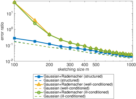
Figure 1: We plot in solid curves the error ratios averaged over 100 trials of the G+R sketching with density $q=0.2$, respectively on the well-conditioned, ill-conditioned and structured linear regressions with varying sketching size $m$. In comparison, the performance of unstructured Gaussian sketching matrix is plotted in dash lines on the same three types of regression problems for reference. The size of the regression problems is set as $n_{1}n_{2}=64^{2}$ by $p=15$.

5.2 Dependence on the number of unknowns $p$

The matrix $\mathbf{A}\in\mathbb{R}^{n_{1}n_{2}\times p}$ is full rank with high probability due to our construction method, thus the number of unknowns $p=\text{rank}(\mathbf{A})$ considering $n_{1},n_{2}\geq p$. We show in Figure 2 the performance of the sketching strategy as the number of unknowns $p$ changes.

1. When the error ratios are relatively small, i.e. under the scale $10^{-1},$ the G+R construction for all three types of programs is shown to have the same dependence as the standard Gaussian matrix on $p,$ or equivalently $\text{rank}(\mathbf{A}),$ given that the slopes are rather similar. This observation is important and provides numerical support for our result Corollary 2.3, that the tensor-structured sketching maintains the same optimal dependence on $\text{rank}(\mathbf{A})$ as conventional Gaussian matrix in unconstrained linear regressions in the small error setting.

2. Larger errors are observed in the solid curves for well and ill-conditioned programs in the large $p$ regime. This is consistent with our unconstrained linear regression theory Corollary 2.3 that the error ratio $\varepsilon$ may change the optimal dependence on $\text{rank}(\mathbf{A})$ to a quadratic dependence when the sketching dimension $m$ is fixed.

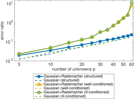
Figure 2: We plot the sketching error ratios with varying number of unknown variables $p$ with fixed ambient dimension $n_{1}n_{2}=64^{2}$ for three different types of linear regression programs. We fix the sketching dimension $m=400$. We compare the performances of the G+R sketching constructed with density $q=0.2$ and standard Gaussian sketching.

5.3 Performance of different sub-Gaussian distributions

In the construction of sketching matrix $\mathbf{S}$ 11, we assume each row is a tensor product of sub-Gaussian random vectors. So far we have employed the sketching design G+R in the numerical experiments above. In this section, we investigate other choices of sub-Gaussian distributions including Rademacher+Rademacher (R+R) and uniform $[-\sqrt{3},\sqrt{3}]$ + uniform $[-\sqrt{3},\sqrt{3}]$ (U+U) and Gaussian+Gaussian (G+G). In Figure 3, for the well-conditioned linear regression only, we test three sketching strategies. All three curves seem to be parallel to that of unstructured sketching matrices, though with different constant intercepts. We think this difference is caused by the factor of maximal $\psi_{2}$ norm $\alpha$ that is implicitly contained in the constant $C$ of 19 in Corollary 2.3. In fact, the parameter $\alpha$ has different values approximately as $1.20,1.34$ and $1.63$ for Rademacher, uniform $[-\sqrt{3},\sqrt{3}]$ and Gaussian random variables respectively. Among all three choices, the R+R design turns out to have the best performance as it has the smallest factor value.

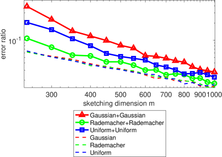
Figure 3: We compare the sketching performances of the G+G, R+R and U+U sketches with varying sketching size $m$ on a well-conditioned linear regression problem of size $n_{1}n_{2}=64^{2}$ by $p=15.$ All three types of random sketches are constructed with density level $q=0.2.$ In addition, we implement the standard Gaussian, Rademacher and uniform $[-\sqrt{3},\sqrt{3}]$ matrices on the same program for reference.

6 Conclusions and future work

In this paper, motived by structured least squares in practical applications, we presented a row-wise tensor-structured sketching design to accelerate the solving procedure. For unconstrained linear regressions, we provided a sharp sketching dimension bound that is derived from the optimal JL property of the proposed sketch. We have also demonstrated a state-of-the-art sketching estimate regarding constrained least squares problems. The result involves the calculation of a $M$-complexity parameter and directly applies to common types of optimizations in different geometry landscapes. In light of the theoretical support to the main result, we developed the analysis for the maximum embedding error of the sketching matrix over a fixed set, with the help of the generic chaining technique. Our theories are then verified by numerical simulations on various choices of sketching matrices and parameter situations.

Future work remains, firstly, considering the suboptimal estimate led by the newly introduced $M$-complexity compared to the classical Gaussian width, we shall seek for a more accessible complexity term to offer a better characterization for sketching constrained optimizations. Secondly, the sketching model in this work considers only the sub-Gaussian random variables, an interesting open problem would be analyzing the sketching property for the randomized FFT-related construction with tensor structure, as such class of sketch enables fast matrix-vector multiplications. The last open problem is inspired by the numerical observations shown in Figure 1 and Figure 2, that the proposed sketching design works better on the tensor-structured programs than unstructured programs. This may suggest that a tighter sketching size estimate could be derived for tensor-structured programs.

Appendix A Proof of Lemma 3.4

Proof of Lemma 3.4.

From Definition 2.4, let $\bm{\mathcal{T}}^{*}$ be an almost optimal skeleton of $\overline{\mathbf{A}\bm{\mathcal{K}}}_{+}\cup\{{\bf 0}\}$ such that

$$\gamma_{1}(\bm{\mathcal{T}}^{*})+\gamma_{2}(\bm{\mathcal{T}}^{*})\leq\frac{13}{12}\,M(\overline{\mathbf{A}\bm{\mathcal{K}}}_{+}).$$ (63)

We then show that $\bm{\mathcal{T}}^{*}+\mathbf{z}\cup\{{\bf 0}\}$ is a skeleton for $\overline{\overline{\mathbf{A}\bm{\mathcal{K}}}_{+}+\mathbf{z}}\cup\{{\bf 0}\}$.

Claim A.1.

$$\overline{\overline{\mathbf{A}\bm{\mathcal{K}}}_{+}+\mathbf{z}}\cup\{{\bf 0}\}\subset\text{conv}(\bm{\mathcal{T}}^{*}+\mathbf{z}\cup\{{\bf 0}\}).$$ (64)

Proof of A.1.

For any $\mathbf{y}\in\overline{\overline{\mathbf{A}\bm{\mathcal{K}}}_{+}+\mathbf{z}},$ there exists an element $\mathbf{y}^{\prime}$ in $\overline{\mathbf{A}\bm{\mathcal{K}}}_{+}$ such that $\mathbf{y}=(\mathbf{y}^{\prime}+\mathbf{z})/\|\mathbf{y}^{\prime}+\mathbf{z}\|_{2}.$ Since $\mathbf{y}^{\prime}\in\overline{\mathbf{A}\bm{\mathcal{K}}}_{+}\subset\text{conv}(\bm{\mathcal{T}}^{*}),$ suppose $\mathbf{y}^{\prime}$ has the expression: $\mathbf{y}^{\prime}=\sum_{i=1}^{I}\alpha_{i}{\bf{t}}_{i},$ where $\{{\bf{t}}_{i}\}_{i\in[I]}\subset\bm{\mathcal{T}}^{*},\alpha_{i}\geq 0,\sum_{i=1}^{I}\alpha_{i}=1$. Then we have a convex construction for $\mathbf{y}$ from the set $\bm{\mathcal{T}}^{*}+\mathbf{z}\cup\{\bf 0\}:$

$$\mathbf{y}=\frac{\mathbf{y}^{\prime}+\mathbf{z}}{\|\mathbf{y}^{\prime}+\mathbf{z}\|_{2}}=\sum_{i=1}^{I}\frac{\alpha_{i}}{\|\mathbf{y}^{\prime}+\mathbf{z}\|_{2}}({\bf{t}}_{i}+\mathbf{z})+(1-\frac{1}{\|\mathbf{y}^{\prime}+\mathbf{z}\|_{2}})\,\bf 0,$$

where the components $\{{\bf{t}}_{i}+\mathbf{z}\}_{i\in[I]},{\bf 0}$ belong to $\bm{\mathcal{T}}^{*}+\mathbf{z}\cup\{\bf 0\}$ and positive weights $(\sum_{i=1}^{I}\frac{\alpha_{i}}{\|\mathbf{y}^{\prime}+\mathbf{z}\|_{2}})+(1-\frac{1}{\|\mathbf{y}^{\prime}+\mathbf{z}\|_{2}})=1$. Note that $\|\mathbf{y}^{\prime}+\mathbf{z}\|_{2}=\sqrt{\|\mathbf{y}^{\prime}\|_{2}^{2}+\|\mathbf{z}\|_{2}^{2}+2\,\langle\mathbf{y}^{\prime},\mathbf{z}\rangle}\geq\sqrt{2}>1,$ so $1/\|\mathbf{y}^{\prime}+\mathbf{z}\|_{2}<1.$

The proof of A.1 is complete. ∎

Based on 15, we then compute $M(\overline{\overline{\mathbf{A}\bm{\mathcal{K}}}_{+}+\mathbf{z}})$ by the $\gamma$-functionals of its skeleton: $\bm{\mathcal{T}}^{*}+\mathbf{z}\cup\{\bf 0\}.$

Next, we aim to bound $\gamma(\bm{\mathcal{T}}^{*}+\mathbf{z}\cup\{\bf 0\})$ by $\gamma(\bm{\mathcal{T}}^{*})$ up to a constant. See the following claim.

Claim A.2.

$$\gamma_{\alpha}(\bm{\mathcal{T}}^{*}+\mathbf{z}\cup\{{\bf 0}\})\leq 12\,\gamma_{\alpha}(\bm{\mathcal{T}}^{*}),\leavevmode\nobreak\ \leavevmode\nobreak\ \text{for}\leavevmode\nobreak\ \leavevmode\nobreak\ \alpha=1,2.$$

Proof of A.2.

By the sub-additivity of $\gamma$-functionals as proved in Lemma 2.1 from [50], we know

$$\begin{array}[]{ll}\gamma_{\alpha}(\bm{\mathcal{T}}^{*}+\mathbf{z}\cup\{{\bf 0}\})&\leq 3\,(\gamma_{\alpha}(\bm{\mathcal{T}}^{*}+\mathbf{z})+\gamma_{\alpha}(\{{\bf 0}\})+\text{diam}(\bm{\mathcal{T}}^{*}+\mathbf{z}\cup\{{\bf 0}\}))\\ &\leq 3\,(\gamma_{\alpha}(\bm{\mathcal{T}}^{*})+\text{diam}(\bm{\mathcal{T}}^{*}+\mathbf{z}\cup\{{\bf 0}\})),\end{array}$$ (65)

due to the fact that $\gamma$-functionals are translation-invariant and $\gamma_{\alpha}(\{{\bf 0}\})=0.$

To evaluate $\text{diam}(\bm{\mathcal{T}}^{*}+\mathbf{z}\cup\{{\bf 0}\})),$ we first have

$$\text{diam}(\bm{\mathcal{T}}^{*}+\mathbf{z}\cup\{{\bf 0}\}))\leq\text{diam}(\bm{\mathcal{T}}^{*}+\mathbf{z})+\text{dist}({\bf 0},\bm{\mathcal{T}}^{*}+\mathbf{z}).$$

As diameter is translation-invariant,

$$\text{diam}(\bm{\mathcal{T}}^{*}+\mathbf{z})=\text{diam}(\bm{\mathcal{T}}^{*}).$$

Also,

$$\begin{array}[]{ll}\text{dist}({\bf 0},\bm{\mathcal{T}}^{*}+\mathbf{z})&=\text{dist}({\bf-z},\bm{\mathcal{T}}^{*})\\ &\leq\text{dist}(-\mathbf{z},{\bf 0})+\text{dist}({\bf 0},\bm{\mathcal{T}}^{*})=\text{dist}({\bf 0},\text{conv}(\bm{\mathcal{T}}^{*}))+\|\mathbf{z}\|_{2}\\ &\leq\text{dist}({\bf 0},\overline{\mathbf{A}\bm{\mathcal{K}}}_{+})+\|\mathbf{z}\|_{2}=2,\quad\text{since}\leavevmode\nobreak\ \overline{\mathbf{A}\bm{\mathcal{K}}}_{+}\subset\text{conv}(\bm{\mathcal{T}}^{*}).\end{array}$$

Hence,

$$\text{diam}(\bm{\mathcal{T}}^{*}+\mathbf{z}\cup\{{\bf 0}\}))\leq\text{diam}(\bm{\mathcal{T}}^{*})+2\leq 3\,\text{diam}(\bm{\mathcal{T}}^{*}).$$ (66)

$\text{diam}(\bm{\mathcal{T}}^{*})\geq 1$ is because $\text{diam}(\bm{\mathcal{T}}^{*})=\text{diam}(\text{conv}(\bm{\mathcal{T}}^{*}))\geq\text{diam}(\overline{\mathbf{A}\bm{\mathcal{K}}}_{+}\cup\{{\bf 0}\})=1.$

Finally, we combine the results of 65 and 66 and obtain

$$\begin{array}[]{ll}\gamma_{\alpha}(\bm{\mathcal{T}}^{*}+\mathbf{z}\cup\{{\bf 0}\})&\leq 3\,(\gamma_{\alpha}(\bm{\mathcal{T}}^{*})+\text{diam}(\bm{\mathcal{T}}^{*}+\mathbf{z}\cup\{{\bf 0}\}))\\ &\leq 3\,(\gamma_{\alpha}(\bm{\mathcal{T}}^{*})+3\,\text{diam}(\bm{\mathcal{T}}^{*}))\leq 12\,\gamma_{\alpha}(\bm{\mathcal{T}}^{*}).\end{array}$$

Note that a set’s diameter is always less than its $\gamma$-functionals.

The proof of A.2 is complete. ∎

Therefore, by A.1, A.2 and 63, we have

$$M(\overline{\overline{\mathbf{A}\bm{\mathcal{K}}}_{+}+\mathbf{z}})\leq(\gamma_{1}+\gamma_{2})(\bm{\mathcal{T}}^{*}+\mathbf{z}\cup\{{\bf 0}\})\leq 12\,(\gamma_{1}+\gamma_{2})(\bm{\mathcal{T}}^{*})=13\,M(\overline{\mathbf{A}\bm{\mathcal{K}}}_{+}).$$

The entire proof for Lemma 3.4 is complete. ∎

References

• [1] Radosław Adamczak and Paweł Wolff. Concentration inequalities for non-lipschitz functions with bounded derivatives of higher order. Probability Theory and Related Fields, 162:531–586, 2013.
• [2] Nir Ailon and Bernard Chazelle. Approximate nearest neighbors and the fast Johnson-Lindenstrauss transform. In STOC’06: Proceedings of the 38th Annual ACM Symposium on Theory of Computing, pages 557–563. ACM, New York, 2006.
• [3] Animashree Anandkumar, Rong Ge, Daniel Hsu, Sham M. Kakade, and Matus Telgarsky. Tensor decompositions for learning latent variable models. Journal of Machine Learning Research, 15:2773–2832, 2014.
• [4] Haim Avron, Huy Nguyen, and David Woodruff. Subspace embeddings for the polynomial kernel. In Advances in Neural Information Processing Systems 27, pages 2258–2266. Curran Associates, Inc., 2014.
• [5] Mohammad Taha Bahadori, Qi (Rose) Yu, and Yan Liu. Fast multivariate spatio-temporal analysis via low rank tensor learning. In Advances in Neural Information Processing Systems 27, pages 3491–3499. Curran Associates, Inc., 2014.
• [6] Casey Battaglino, Grey Ballard, and Tamara G. Kolda. A practical randomized CP tensor decomposition. SIAM J. Matrix Anal. Appl., 39(2):876–901, 2018.
• [7] Léon Bottou, Frank E. Curtis, and Jorge Nocedal. Optimization methods for large-scale machine learning. SIAM Review, 60(2):223–311, 2018.
• [8] Jean Bourgain, Sjoerd Dirksen, and Jelani Nelson. Toward a unified theory of sparse dimensionality reduction in euclidean space. Geometric and Functional Analysis, 25:1009–1088, 2015.
• [9] Sébastien Bubeck. Convex optimization: Algorithms and complexity. Foundations and Trends in Machine Learning, 8(3-4):231–357, 2015.
• [10] Moses Charikar, Kevin C. Chen, and Martin Farach-Colton. Finding frequent items in data streams. Theor. Comput. Sci., 312(1):3–15, 2004.
• [11] Ke Chen, Qin Li, Kit Newton, and Steve Wright. Structured random sketching for PDE inverse problems. arXiv e-prints, September 2019.
• [12] Dehua Cheng, Richard Peng, Yan Liu, and Ioakeim Perros. SPALS: fast alternating least squares via implicit leverage scores sampling. In Advances in Neural Information Processing Systems 29: Annual Conference on Neural Information Processing Systems 2016, December 5-10, 2016, Barcelona, Spain, pages 721–729, 2016.
• [13] Kenneth L. Clarkson and David P. Woodruff. Low rank approximation and regression in input sparsity time. In Proceedings of the Forty-fifth Annual ACM Symposium on Theory of Computing, STOC ’13, pages 81–90, New York, NY, USA, 2013. ACM.
• [14] Nadav Cohen, Or Sharir, and Amnon Shashua. On the expressive power of deep learning: A tensor analysis. volume 49 of Proceedings of Machine Learning Research, pages 698–728, Columbia University, New York, New York, USA, 23–26 Jun 2016. PMLR.
• [15] Anirban Dasgupta, Ravi Kumar, and Tamás Sarlós. A sparse Johnson-Lindenstrauss transform. In STOC’10—Proceedings of the 2010 ACM International Symposium on Theory of Computing, pages 341–350. ACM, New York, 2010.
• [16] Lieven De Lathauwer, Bart De Moor, and Joos Vandewalle. A multilinear singular value decomposition. SIAM Journal on Matrix Analysis and Applications, 21(4):1253–1278, 2000.
• [17] Huaian Diao, Zhao Song, Wen Sun, and David P. Woodruff. Sketching for Kronecker Product Regression and P-splines. In International Conference on Artificial Intelligence and Statistics, AISTATS, pages 1299–1308, 2018.
• [18] Petros Drineas, Michael W. Mahoney, and S. Muthukrishnan. Sampling algorithms for l2 regression and applications, 2006.
• [19] Mário A. T. Figueiredo, Robert D. Nowak, and Stephen J. Wright. Gradient projection for sparse reconstruction: Application to compressed sensing and other inverse problems. IEEE Journal of Selected Topics in Signal Processing, 1(4):586–597, 2007.
• [20] Martin Genzel and Christian Kipp. Generic Error Bounds for the Generalized Lasso with Sub-Exponential Data. arXiv e-prints, April 2020.
• [21] Yehoram Gordon. Some inequalities for gaussian processes and applications. Israel Journal of Mathematics, 50:265–289, 12 1985.
• [22] Friedrich Götze, Holger Sambale, and Arthur Sinulis. Concentration inequalities for polynomials in alpha-sub-exponential random variables. Electronic Journal of Probability, 26:1 – 22, 2021.
• [23] Peter D. Hoff. Multilinear tensor regression for longitudinal relational data. Ann. Appl. Stat., 9(3):1169–1193, 09 2015.
• [24] Ruhui Jin, Tamara G. Kolda, and Rachel Ward. Fast Johnson-Lindenstrauss transforms via Kronecker products. arXiv e-prints, September 2019.
• [25] William B. Johnson and Joram Lindenstrauss. Extensions of Lipschitz mappings into a Hilbert space. volume 26 of Contemp. Math., pages 189–206. Amer. Math. Soc., Providence, RI, 1984.
• [26] Purushottam Kar and Harish Karnick. Random feature maps for dot product kernels. volume 22 of Proceedings of Machine Learning Research, pages 583–591, La Palma, Canary Islands, 21–23 Apr 2012. PMLR.
• [27] Tamara Kolda and Brett Bader. Tensor decompositions and applications. SIAM Review, 51(3):455–500, 2009.
• [28] Kasper G. Larsen and Jelani. Nelson. Optimality of the Johnson-Lindenstrauss Lemma. In 2017 IEEE 58th Annual Symposium on Foundations of Computer Science (FOCS), pages 633–638, Oct 2017.
• [29] Rafal Latała. Estimates of moments and tails of Gaussian chaoses. The Annals of Probability, 34(6):2315 – 2331, 2006.
• [30] Xingguo Li, Jarvis Haupt, and David Woodruff. Near optimal sketching of low-rank tensor regression. In Advances in Neural Information Processing Systems 30, pages 3466–3476. Curran Associates, Inc., 2017.
• [31] Osman A. Malik and Stephen Becker. Guarantees for the kronecker fast johnson-lindenstrauss transform using a coherence and sampling argument. Linear Algebra and its Applications, 602:120–137, October 2020.
• [32] Michela Meister, Tamas Sarlos, and David Woodruff. Tight dimensionality reduction for sketching low degree polynomial kernels. In H. Wallach, H. Larochelle, A. Beygelzimer, F. dAlché Buc, E. Fox, and R. Garnett, editors, Advances in Neural Information Processing Systems 32, pages 9475–9486. Curran Associates, Inc., 2019.
• [33] Shahar Mendelson, Alain Pajor, and Nicole Tomczak-Jaegermann. Reconstruction and subgaussian operators in asymptotic geometric analysis. Geometric and Functional Analysis, 17:1248–1282, 11 2007.
• [34] Xiangrui Meng and Michael W. Mahoney. Low-distortion subspace embeddings in input-sparsity time and applications to robust linear regression. In Proceedings of the 45th Annual ACM Symposium on Theory of Computing, pages 91–100. ACM, 2013.
• [35] Jorge Nocedal and Stephen J. Wright. Numerical optimization. Springer series in operations research and financial engineering. Springer, New York, NY, 2. ed. edition, 2006.
• [36] Guillermo Ortiz-Jimenez, Mario Coutino, Sundeep Prabhakar Chepuri, and Geert Leus. Sparse sampling for inverse problems with tensors. IEEE Transactions on Signal Processing, 67(12):3272–3286, 2019.
• [37] Rasmus Pagh. Compressed matrix multiplication. ACM Transactions on Computation Theory, 5, 08 2011.
• [38] Ninh Pham and Rasmus Pagh. Fast and scalable polynomial kernels via explicit feature maps. In Proceedings of the 19th ACM SIGKDD International Conference on Knowledge Discovery and Data Mining, KDD ’13, pages 239–247, New York, NY, USA, 2013. ACM.
• [39] Mert Pilanci and Martin J. Wainwright. Randomized sketches of convex programs with sharp guarantees. IEEE Transactions on Information Theory, 61(9):5096–5115, 2015.
• [40] Mert Pilanci and Martin J. Wainwright. Iterative hessian sketch: Fast and accurate solution approximation for constrained least-squares. Journal of Machine Learning Research, 17(53):1–38, 2016.
• [41] Beheshteh T. Rakhshan and Guillaume Rabusseau. Tensorized Random Projections. arXiv e-prints, page arXiv:2003.05101, March 2020.
• [42] Vladimir Rokhlin and Mark Tygert. A fast randomized algorithm for overdetermined linear least-squares regression. Proceedings of the National Academy of Sciences, 105(36):13212–13217, 2008.
• [43] Mark Rudelson and Roman Vershynin. On sparse reconstruction from Fourier and Gaussian measurements. Comm. Pure Appl. Math., 61(8):1025–1045, 2008.
• [44] Yiming Sun, Yang Guo, Joel A Tropp, and Madeleine Udell. Tensor random projection for low memory dimension reduction. In NeurIPS Workshop on Relational Representation Learning, 2018.
• [45] Michel Talagrand. Majorizing measures: the generic chaining. Ann. Probab., 24(3):1049–1103, 07 1996.
• [46] Michel Talagrand. The Generic Chaining: Upper and Lower Bounds of Stochastic Processes. Springer Monographs in Mathematics. Springer Berlin Heidelberg, 2005.
• [47] Robert Tibshirani. Regression shrinkage and selection via the lasso. Journal of the Royal Statistical Society. Series B (Methodological), 58(1):267–288.
• [48] Joel A. Tropp. Improved analysis of the subsampled randomized hadamard transform. Adv. Data Sci. Adapt. Anal., 3(1-2):115–126, 2011.
• [49] Roman Vershynin. High-Dimensional Probability: An Introduction with Applications in Data Science. 09 2018.
• [50] Vincent Q. Vu and Jing Lei. Squared-norm empirical processes. Statistics & Probability Letters, 150:108–113, 2019.
• [51] David Woodruff. Sketching as a tool for numerical linear algebra. Foundations and Trends in Theoretical Computer Science, 10, 11 2014.