The mid-infrared Leavitt Law for Classical Cepheids in the Magellanic Clouds
Abstract
The Cepheid Leavitt Law (LL), also known as the Period-Luminosity relation, is a crucial tool for assembling the cosmic distance ladder. By combining data from the OGLE-IV catalogue with mid-infrared photometry from the Spitzer Space Telescope, we have determined the m and m LLs for the Magellanic Clouds using fundamental-mode Classical Cepheids. Mean magnitudes were determined using a Monte Carlo Markov Chain (MCMC) template fitting procedure, with template light curves constructed from a subsample of these Cepheids with fully-phased, well-sampled light curves. The dependence of the Large Magellanic Cloud LL coefficients on various period cuts was tested, in addition to the linearity of the relationship. The zero point of the LL was calibrated using the parallaxes of Milky Way Cepheids from the Hubble Space Telescope and Gaia Data Release 2. Our final calibrated relations are and .
keywords:
stars: variables: Cepheids – Magellanic Clouds – infrared: stars1 Introduction
Since its initial discovery around a century ago, the Cepheid Leavitt Law (Leavitt 1908; Leavitt & Pickering 1912), also known as the Period-Luminosity relation, has proven to be an imperative tool for measuring astronomical distances. The Leavitt Law (LL) relates the luminosity of a Cepheid to its pulsation period, revealing that Cepheids with longer periods are intrinsically brighter than their shorter period counterparts. Thus, Cepheid variables play a vital role as distance indicators; in particular, their LL is often used as the first rung of the traditional cosmic distance ladder, which in turn can be used to measure the Hubble constant, . In recent years, a growing discrepancy between local- and early-Universe measurements of has arisen (see Riess 2019 for a review). Therefore, reducing the uncertainties associated with the Cepheid LL will prove essential for understanding the reason behind this discrepancy.
In her pioneering work, Henrietta Leavitt determined the LL for 25 Cepheids in the Small Magellanic Cloud (Leavitt & Pickering, 1912). Since then, a large and growing body of literature has emerged, with many Local Group galaxies now possessing their own LL (e.g.: MW, Tammann et al. 2003; NGC 6822, Madore et al. 2009a; M33, Scowcroft et al. 2009; M31, Kodric et al. 2015). Of particular importance are the Large and Small Magellanic Clouds (LMC and SMC, respectively). These galaxies are relatively nearby, making them excellent targets for stellar population studies as their individual stars can be resolved. Notably, they each have a substantial Cepheid population, with the Optical Gravitational Lensing Experiment (OGLE) (Udalski et al., 1999) cataloguing fundamental-mode Classical Cepheids across both galaxies. Due to the LMC being used as the current anchor galaxy for the extragalactic distance scale, its Cepheid population has been studied extensively. Although the SMC is not used in anchoring the distance scale, it serves as a key galaxy for examining the effect of metallicity on the LL, as it is more metal-poor than both the LMC and Milky Way (MW).
The LL for the Magellanic Clouds has been studied at many wavelengths, from the optical through to the mid-infrared. Numerous studies have been performed at optical wavelengths (e.g. Gieren et al. 2005; Sandage et al. 2009; Ngeow et al. 2015; Groenewegen 2018). Fouqué et al. (2007) suggested that the LL is universal, as they found no significant difference in the slopes of the MW and LMC LL for various bands (from to ). In the near-infrared, Ripepi et al. (2016) used data from the VISTA survey of the Magellanic Clouds (VMC) (Cioni et al., 2011) to determine the LLs for 4172 SMC Classical Cepheids. For the LMC, a near-infrared synoptic survey of its central region was performed by Macri et al. (2015) to obtain the LLs for 1417 LMC Classical Cepheids. At mid-infrared (mid-IR) wavelengths, the Carnegie Hubble Program (CHP) performed observations of fundamental-mode Classical Cepheids using the Spitzer Space Telescope to determine the m and m LLs for 37 MW (Monson et al. 2012, hereafter M12), 85 LMC (Scowcroft et al. 2011, hereafter S11) and 90 SMC (Scowcroft et al. 2016b, hereafter S16) Cepheids. The observations for these Cepheids were designed to uniformly sample the pulsation cycle, resulting in exquisite light curves and highly-precise mean magnitudes. Complementary analyses of the Spitzer SAGE (Surveying the Agents of a Galaxy’s Evolution) (Meixner et al., 2006) catalogue used much larger samples of Cepheids than the CHP to determine the mid-IR LL for the LMC and SMC, at the expense of a much coarser sampling of the light curves (one or two epochs only), thus leaving more significant uncertainties in the mean magnitudes (Ngeow & Kanbur 2008; Ngeow et al. 2009; Ngeow & Kanbur 2010).
In this study, we use mid-IR data of Cepheids, as observations at these longer wavelengths have several fundamental advantages over optical wavelengths. First, the effects of interstellar extinction are substantially reduced in the infrared, with the Spitzer m band extinction being around 20 times smaller than the extinction in the band (Indebetouw et al., 2005). Second, infrared Cepheid light curves have smaller amplitudes than their optical analogues. This phenomenon occurs because the mid-IR is situated in the Rayleigh–Jeans tail of the stellar spectrum, resulting in minimal temperature effects on the light curve and a more sinusoidal shape. Finally, the dispersion of the mid-IR LL is smaller and its slope is steeper than its optical counterparts, also arising from these wavelengths being dominated by radius variations rather than temperature variations. Consequently, magnitudes inferred from a mid-IR LL will carry smaller systematic uncertainties than those inferred from optical relations (S16).
The work presented in this paper combines the CHP sample of Cepheids from S11 and S16 with the Spitzer SAGE survey to obtain m and m magnitudes for all known fundamental-mode Classical Cepheids in the Magellanic Clouds, as provided in the OGLE-IV catalogue (Soszyński et al., 2017). The previously mentioned studies that used the SAGE catalogue (Ngeow & Kanbur 2008; Ngeow et al. 2009; Ngeow & Kanbur 2010) only used the OGLE-III catalogue of Cepheids. Since then, OGLE have discovered more Cepheids in the Magellanic Clouds, resulting in the OGLE-IV catalogue. Thus, our work is the most comprehensive mid-IR Cepheid study in the Magellanic Clouds to date. In a separate companion paper (Chown et al. 2020, in prep), we exploit this highly complete and refined catalogue of Cepheid distances to map the 3D distribution of the Magellanic System.
The paper is organised as follows: Section 2 describes the datasets used in this work. In Section 3 we outline the fully-automated photometry pipeline that was developed to process the data. Section 4 describes our template light curve construction and fitting methods. In Section 5 we present our mid-IR catalogue of Magellanic Cloud Cepheids. In Section 6 we assess the dependency of the LL on sample characteristics, and also compare our relations to the literature. Section 6.3 gives our final adopted LL and its zero point calibration. We present our conclusions in Section 7.
Throughout this paper, the term “Cepheid” will refer to Type-I Classical Cepheids pulsating in the fundamental mode.
2 Data & Observations
| LMC | SMC | |||
| Cal | Complete | Cal | Complete | |
| 85 | 2477 | 90 | 2754 | |
| Median | 24 | 3 | 12 | 4 |
| Period range (d) | ||||
| Mean period (d) | 25.62 | 5.22 | 22.08 | 3.49 |
The data used in this work are from Spitzer, which launched in 2003 and recently ceased operations in January 2020. Onboard Spitzer was the Infrared Array Camera (IRAC, Fazio et al., 2004), which initially operated simultaneously at four mid-infrared wavelengths (3.6 m, 4.5 m, 5.8 m and 8.0 m) during its “cold” mission. Once its cryogenic fuel was exhausted in 2009, Spitzer entered its “warm mission” phase, operating only at the two shorter wavelengths, 3.6 m and 4.5 m. We combine data from both the cold and warm missions, using only the data at 3.6 m and 4.5 m (henceforth denoted as and , respectively).
We use data from both the CHP sample (S11; M12; S16) of Cepheids and the Spitzer SAGE survey (Meixner et al. 2006; Gordon et al. 2011; Riebel et al. 2015). While the CHP sample has fully-phased well-sampled observations for every Cepheid (number of observations for the LMC and 12 for the SMC), the SAGE data only provides a few observations (median number of observations are 3 and 4 for the LMC and SMC, respectively) that do not uniformly sample the light curve. Therefore, in order to obtain precise mean magnitudes of the Cepheids with sparsely sampled light curves, we have developed and applied a template light curve fitting procedure. The templates are constructed from the CHP Cepheids, hereafter referred to as the “calibrating sample”. These templates are then fit to the sample of all known fundamental mode Cepheids in the Magellanic Clouds, hereafter referred to as the “complete sample”. Sample statistics for the calibrating and complete samples are provided in Table 1.
2.1 Calibrating sample
The calibrating sample have photometric data taken as part of the CHP (Freedman et al., 2011). Our sample consists of 85 LMC Cepheids (PI Freedman, Program IDs: 61000, 04, 05, 06, 07; S11) with periods () in the range days, and 90 SMC Cepheids (PI Madore, Program ID 70010; S16) with days. All observations were taken during Spitzer’s warm mission. Each observation consists of ten frames (five in each of the two wavelengths) where the Cepheid is in the field of view. Each frame has a frame time of 2.0 s, resulting in an effective per-pixel integration time of 1.2 s. A medium-scale, five-point Gaussian dither pattern was used to reduce the effects of cosmic rays hitting the detector and also improves the S/N for the Cepheid.
Cepheids with days have full-phase coverage, with approximately equally spaced observations over one pulsation cycle. These observations were taken using deterministic sampling in approximately steps for the LMC and steps for the SMC. A full discussion and justification of this observing strategy is given in the appendix of S11. To summarise, deterministic sampling requires fewer observations than random sampling to achieve the same precision, as the error on the mean follows compared to random sampling where , for observations. For the deterministic sampling strategy and described above, the error on the mean magnitude for each Cepheid reduces by a factor of and for the LMC and SMC, respectively, compared to random sampling.
The shorter period Cepheids with days could not be observed in such a tightly phased way, as this would overburden the Spitzer schedule. Instead, each observation epoch was separated by days to ensure minimal overlap of phase points, thus reducing the likelihood of redundant data. The uncertainties on the magnitudes for these Cepheids follow , as their light curve is randomly sampled.
2.2 Complete sample
2.2.1 Sample selection
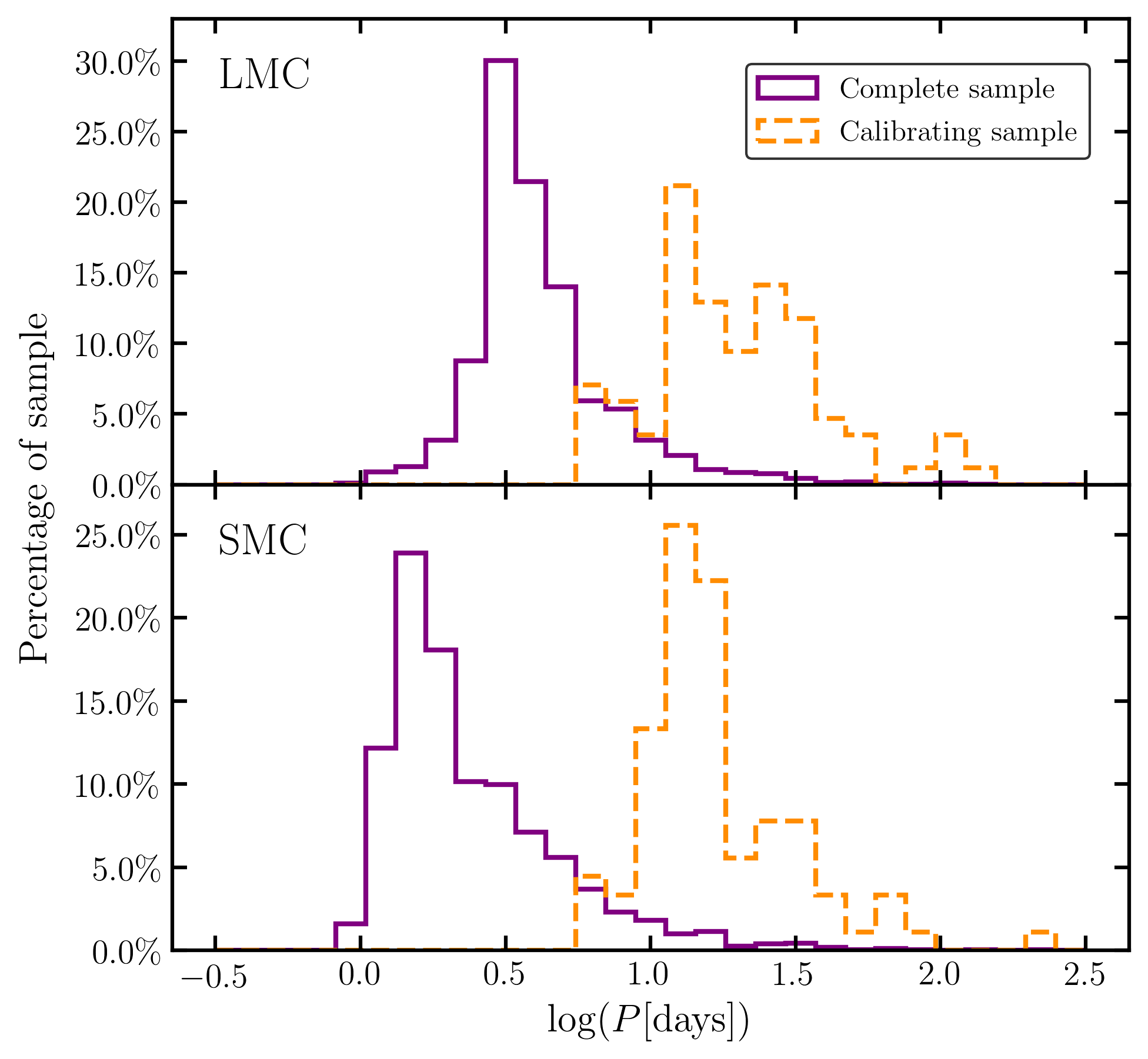
Our complete sample contains 2477 LMC and 2754 SMC fundamental-mode Classical Cepheids. These are all the known Cepheids of this type found in the Magellanic Clouds, as given in the OGLE-IV catalogue of variable stars (Soszyński et al., 2017). Figure 1 shows the period distribution for both the complete and calibrating samples, where the periods have been taken from the OGLE-IV catalogue (Soszyński et al., 2017). For our work, we adopt these periods as they are extremely precise, with uncertainties on the order of s. For the complete sample, shown by the purple solid lines in Figure 1, both galaxies have distributions that are skewed towards short periods, with average periods of 5.22 and 3.49 days for the LMC and SMC populations, respectively. As a result of the CHP selecting Cepheids that were bright, we see that the calibrating sample, shown by the orange dashed lines, occupies the long period end of the complete sample distribution. Along with the period, the OGLE catalogue also provides the RA and Dec positions for each Cepheid. These coordinates are adopted in this work and used to determine the positions of the Cepheids in the SAGE images.
2.2.2 Photometric data
The mid-IR observations for the complete sample of Cepheids were taken as part of the Spitzer SAGE legacy program. SAGE performed a uniform and unbiased imaging survey of the LMC (Meixner et al., 2006), SMC and Magellanic Bridge (MB) (Gordon et al., 2011). The LMC footprint is shown in figure 3 of Meixner et al. (2006), while the SMC footprint is shown in figure 2 of Gordon et al. (2011). The SAGE observations were carried out in 2005 during Spitzer’s cold mission at two epochs separated by approximately three months. A follow-up program to SAGE, SAGE-Var (Riebel et al., 2015), was conducted between August 2010 and June 2011 during the warm mission. These observations focused on the bar of the LMC and the central region of the SMC, providing up to an additional four epochs for these regions. Figures 1 and 2 of Riebel et al. (2015) show the SAGE-Var footprint for the LMC and SMC, respectively.
As a result of the extensive spatial coverage of the SAGE survey, each SAGE Cepheid has between two and six epochs of observation, depending on its location within its host galaxy, providing several phase points of each mid-IR light curve. Although SAGE performed its observations at all four Spitzer wavelengths, we only use the and data so that the CHP and SAGE observations can be combined. In addition to providing observations for Cepheids in the complete sample, SAGE also yields additional observations for the calibrating Cepheids, since these Cepheids are a subset of the complete sample.
3 Photometry pipeline
We developed a fully-automated photometry pipeline to obtain intensity-averaged mean magnitudes and light curves for each Cepheid in our sample. While the photometry for the calibrating and complete samples was obtained using an identical pipeline to ensure consistent analysis, the determination of the intensity-averaged mean magnitudes and light curves differs between the two samples, due to the calibrating sample having vastly more observations than the complete sample. For the calibrating sample, we used GLOESS fitting (further details in Section 3.3) to obtain the mid-IR mean magnitudes and light curves. For the complete sample, we developed and applied a template fitting procedure, as described in Section 4.1, where the templates were constructed from the fully-phased well-sampled light curves of the calibrating sample.
The input files are individual Basic Calibrated Data (CBCD) FITS images downloaded from the Spitzer Heritage Archive (SHA). These images were initially processed using the Spitzer processing pipeline, Version S19.2. To perform the photometry, we used the DAOPHOT/ALLSTAR/ALLFRAME (Stetson 1987; Stetson &
Harris 1988; Stetson 1994) packages, kindly provided by Peter Stetson. Our photometry pipeline is written entirely in Python, using the pexpect package to control the photometry packages. The code used for this work is publicly available111https://github.com/abichown/DAOPHOT-Scripts. The remainder of this section outlines the main steps of our fully-automated photometry pipeline.
3.1 PSF photometry
Initial star lists for each CBCD frame were created using the DAOPHOT FIND routine, with a and detection threshold for the LMC and SMC, respectively. A lower threshold value for the SMC was required as it is the more distant galaxy, resulting in fainter magnitudes which are harder to detect. Aperture photometry was then performed using the PHOT routine to obtain rough instrumental magnitudes. A 3 pixel aperture radius and sky annulus from 12 to 20 pixels was used. This aperture radius is smaller than the standard IRAC Vega system value, as given in Reach et al. (2005, hereafter R05), but this difference is corrected for (see Section 3.2). A smaller aperture radius was preferred as some Cepheids have neighbours within a 10 pixel radius; if the larger aperture were used instead, these neighbours would contaminate the magnitude measurement of our Cepheid. The instrumental magnitudes computed at this stage are only initial estimates as some fields are fairly crowded, which causes the sky annulus to be contaminated.
Next, we created a median image by combining all available CBCD images that contained the target Cepheid. Due to the scheduling and design of the observations, there are two fields for each Cepheid: one field contains the target Cepheid, referred to here as the “on-target” field, and the other does not. For the LMC Cepheids, there are 240 (24 epochs 5 dithers 2 wavelengths) on-target frames, while there are 120 (the same as for the LMC but with 12 epochs) on-target frames for the SMC Cepheids. Initial coordinate transformations between each of the on-target frames were determined using DAOMATCH, which uses the 30 brightest stars in each image to compute these transformations. These initial transformations are then refined using DAOMASTER, which uses all of the stars in the image to improve the DAOMATCH transformations. The median image was created by passing these coordinate transformations through the MONTAGE2 package.
The creation of the median image serves two purposes: it is used to create a master star list and is also used to create a Point Spread Function (PSF) model. Due to the stacking of a large number of frames, the signal-to-noise (S/N) ratio is much greater for the median image than for the individual CBCD frames. This high S/N ratio is beneficial for both the creation of a PSF model and obtaining a master star list. We obtained the master star list by performing FIND and PHOT on the median image. The detection threshold was increased to 20, as this was determined to be the optimal threshold which ensured the majority of stars were detected without a significant number of false detections. The master star list contains coordinates for all stars in the on-target field and is used in subsequent steps of the pipeline.
In addition to the master star list, a suitable PSF model was created from the median image. When the stellar field is crowded, PSF photometry is vastly superior to aperture photometry, as multiple PSF models can be fit simultaneously to groups of overlapping stars. The creation of the PSF model is the most crucial step of the photometry pipeline, as the model must be representative of all the stars in the image so that accurate magnitudes can be obtained.
To create the PSF model, a sample of “good” stars are selected as input; these stars should be bright and relatively free from crowding. The 20 brightest stars in the master star list that were not saturated were initially selected as PSF stars. These stars are then accepted or rejected depending on their position in the median image; stars are rejected if they are too close to the edge of the frame, as there are less individual CBCD images at the edges of the median image, resulting in a lower S/N. A star was also rejected if it had any neighbours that could affect its use as a PSF star. After these tests, the resulting list of stars was passed to the PSF routine to create the PSF model, with the smallest “Chi” value222DAOPHOT II User’s Manual, Peter Stetson being chosen as the final model.
Using the ALLSTAR package and providing it with the PSF model previously created, we obtain instrumental magnitudes via PSF photometry for each individual CBCD image. While the magnitudes from ALLSTAR are reasonable, the uncertainties can be reduced using ALLFRAME. ALLFRAME works in a similar way to ALLSTAR, except that the pixel positions of the stars are fixed. From ALLFRAME, the pipeline outputs instrumental PSF magnitudes for all stars in every individual CBCD image, which includes the magnitude of the target Cepheid.
3.2 Photometric calibration
The instrumental PSF magnitudes from our photometry pipeline were calibrated to the standard IRAC Vega system (R05). In addition, we applied corrections based on a star’s position in the image, as recommended in the IRAC handbook (Version 2.1.2). These steps are essential to ensure we obtain high precision photometry. To this end, four calibration steps were applied to our photometry results: an aperture correction, a zero point correction, a location correction, and a pixel-phase response correction.
We first calibrated our magnitudes to the standard IRAC Vega system (R05). We corrected the standard zero points used by DAOPHOT to IRAC zero points of 17.30 and 16.81 for the and band, respectively. An aperture correction of 1.1132 for the band and 1.1126 for the band (S. Carey, private communication) were applied to convert to the same aperture system as R05.
To ensure we have high-precision photometry, we also corrected for effects due to the different responses of the pixels across the detector. These corrections are small but it is important to correct for all possible sources of photometric error. The two corrections that were applied account for both the star’s pixel location in the image and also its precise location within that pixel. The need to correct the magnitude based on the star’s location in the array is due to two effects that are not corrected for by flat-fielding: the first being significant scattering and distortion in the images, and the second being a variation in the effective filter bandpass as a function of the angle of incidence333https://irsa.ipac.caltech.edu/data/SPITZER/docs/irac/iracinstrumenthandbook/19/#_Toc410728307.
The location correction accounts for the star’s position in the image. To apply the location correction, wavelength-specific correction images were downloaded from the Spitzer website444https://irsa.ipac.caltech.edu/data/SPITZER/docs/irac/calibrationfiles/locationcolor/. For each star, its position was obtained and the corresponding correction value from the correction image was also found. The measured flux of the star is then multiplied by this correction factor. These corrections are small, with the location-corrected magnitude being between 0.022 mag brighter and 0.067 mag dimmer than the uncorrected magnitude.
The pixel-phase correction accounts for the fact that a star’s precise location within a pixel affects the response of that pixel to the star. This effect is believed to be caused primarily by intra-pixel quantum efficiency variations (Mighell
et al., 2008). To correct for this effect, IDL code is available555https://irsa.ipac.caltech.edu/data/SPITZER/docs/irac/calibrationfiles/pixelphase/, which we converted to Python for consistency with the rest of our pipeline. A correction value is obtained and applied for each individual star. The pixel-phase corrected magnitude can be between 0.052 mag brighter and 0.042 mag dimmer than the uncorrected magnitude. Completion of this final step of the calibration procedure yields calibrated magnitudes on the standard IRAC Vega system for all calibrating Cepheids. To determine the average uncertainty on the magnitudes obtained, we took a randomly chosen frame and computed the average uncertainty of all its stars, not just the Cepheids. We found that the typical uncertainty on a single photometric point was mag.
3.3 GLOESS fitting
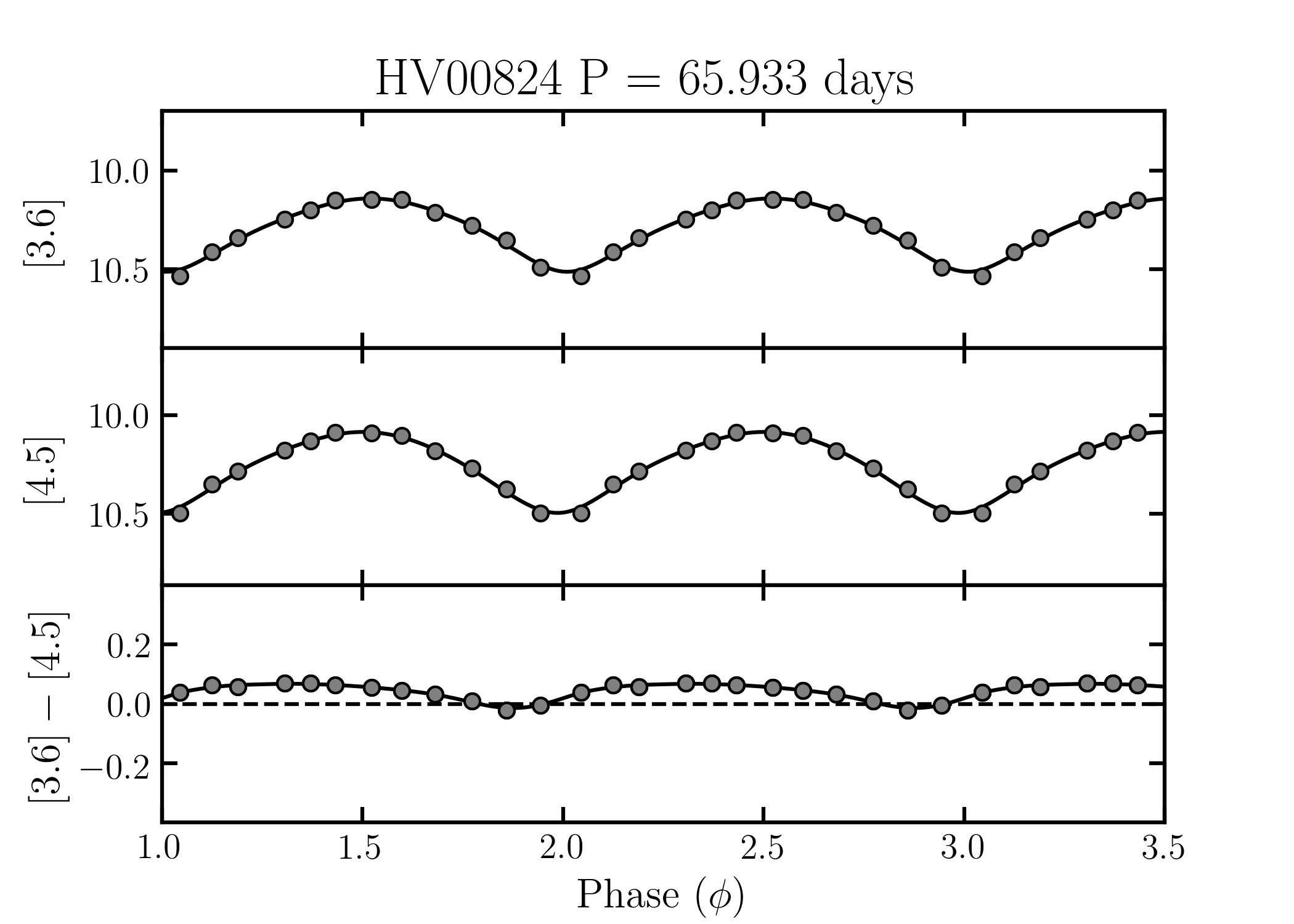
The LMC and SMC Cepheids in the calibrating sample have 24 and 12 epochs of observation, respectively. Due to the five-dither pattern implemented in the scheduling of observations, each epoch has five magnitude measurements of the target Cepheid. We computed the intensity-averaged magnitude for each epoch as the uncertainty weighted mean of the fluxes, with weightings given by the inverse variance. The typical uncertainty on the magnitude at each epoch of observation is mag. These magnitudes were then phased using the pulsation periods from OGLE and the resulting light curves were fit with GLOESS, a Gaussian local estimation algorithm (Persson et al., 2004). GLOESS fits the data via a local regression method using a second-order polynomial. The algorithm produces a smooth curve through the and observations independently by interpolating between each two consecutive data points using a Gaussian window. The colour curve is computed as the difference between the and curves.
The mean magnitude of the Cepheid in each photometric band is determined as the intensity-averaged value of its GLOESS fitted curve across one entire pulsation cycle. Thus, the mean magnitude does not necessarily lie exactly halfway between the minimum and maximum value of the curve. Instead, its value depends on the fraction of one entire pulsation cycle that is spent at brighter magnitudes compared to the amount spent at fainter magnitudes. Similarly, the mean colour is computed as the average value of the colour curve across one complete cycle. For both the light curves and colour curve, the amplitude is computed as the maximum minus the minimum magnitude for the GLOESS curve, not the difference between the maximum and minimum phase points.
Example light and colour curves obtained are shown in Figure 2 for the SMC Cepheid HV00824. The top two panels of Figure 2 show the and light curves, while the bottom panel shows the colour curve. The uncertainties on the individual epoch measurements for the light curves are comparable to the size of the points. We confirm that the 12 equally-spaced observations allow for excellent determination of the Cepheid’s light curve and hence its mean magnitude. In the bottom panel, we observe how the infrared colour curve illustrates the destruction and formation of CO in the Cepheid’s atmosphere (Scowcroft et al., 2016a).
We compared our mean magnitudes for these calibrating Cepheids to those from S11 and S16 for an identical sample of Cepheids. Combining the LMC and SMC samples, we computed the mean difference in magnitude as mag and mag for the and band, respectively. Differences between these results could be due to differences between our pipeline and the one used by S11 and S16, such as the use of different versions of the Spitzer processing pipelines or that we used PSF photometry rather than PRF photometry.
3.4 SAGE photometry pipeline
In order to process the SAGE data, we made small modifications to the photometry pipeline described in Sections 3.1 and 3.2 to account for the differences between the SAGE data and the CHP calibrating data. As much as possible, we kept the pipeline the same to ensure that the photometry was obtained consistently for both datasets. As with the calibrating sample, the SAGE photometry pipeline puts magnitudes on the standard IRAC Vega photometric system. The main modifications that were made are the following:
-
1.
Instead of working with the individual CBCD images and using
MONTAGE2to create a medianed image, we usedMOPEX(Makovoz & Khan, 2005) to create mosaics of an entire AOR. This process conserves flux, hence we can use these mosaics to measure magnitudes. -
2.
The
DAOPHOTparameters for theFINDroutine were updated to account for the SAGE images being mosaics rather than single CBCD images. -
3.
The
DAOPHOTparameters for thePHOTroutine were updated to account for the change in pixel size. Previously, the pixel size of the individual CBCDs were , while the SAGE mosaic images have a pixel size of . Rather than using a 3 px aperture with a px sky annulus, a 10 px aperture with px sky annulus was used. -
4.
Many of the mosaics - particularly in the central regions of each galaxy - are extremely crowded and it is therefore not appropriate to obtain an individual PSF model for each mosaic. Therefore, we used the mosaic image of an uncrowded region in each galaxy to produce a PSF model for each wavelength. We also used the PSF stars that created each PSF model to compute the corresponding aperture correction.
-
5.
The calibrating sample were observed entirely during Spitzer’s warm mission. However, as the SAGE observations were carried out during both cold and warm missions, we updated the photometry pipeline to apply the appropriate calibration procedure depending on when the observations were taken.
4 Template light curve fitting methods
The calibrating Cepheids have well-sampled light curves in both the optical and mid-IR bands, making them excellent for use in creating template light curves. These templates can then be applied to the complete sample of Cepheids in the OGLE-IV catalogue in combination with our photometric measurements from the SAGE images, to obtain mean-light magnitudes in the mid-infrared. The template fitting procedure is a necessary step as the data available from SAGE are sparse and do not uniformly sample the Cepheid light curve. Applying a template to the available phase points produces significantly more precise mean magnitudes and colours compared to just averaging the available magnitude measurements. We now describe our template light curve construction process as well as the method for fitting the templates.
4.1 Template light curve construction
| Grouping method | Subsample characteristic | MAD |
| Host galaxy | LMC | 0.065 |
| SMC | 0.079 | |
| Wavelength | 0.064 | |
| 0.071 | ||
| Period | 0.133 | |
| 0.094 | ||
| 0.071 | ||
| 0.055 | ||
| 0.052 | ||
| 0.047 | ||
| Mid-IR colour | 0.049 | |
| 0.059 | ||
| 0.078 | ||
| 0.076 | ||
| 0.077 | ||
| 0.093 |
Template light curves that are representative of a population of Cepheids can be obtained by compiling the observations from a large number of these Cepheids into a single light curve. In order to compile data in this way, a necessary step was to modify the way in which our data were phased. Thus far, the observations were phased using the periods from OGLE-IV (Soszyński et al., 2015) using
| (1) |
where is the phase, is the Julian Date of the observation and is the period. However, phasing in this way does not allow for data from multiple Cepheids to be compiled together as there is no consistent zero-phase point. To set the zero point of their phasing, Soszynski et al. (2005) use the time of maximum brightness. However, due to the Hertzsprung progression (Hertzsprung, 1926), Cepheids with periods between 6 and 16 days exhibit a secondary bump in their optical light curves near maximum brightness. Therefore, Inno et al. (2015) argue that a more robust zero-phase point is the phase of the mean magnitude along the rising branch of the light curve, as it is not affected by this phenomena. Since approximately of our complete sample are within this period range, we choose to follow the approach of Inno et al. (2015), anchoring our observations to the time of mean magnitude along the rising branch, . Equation 1 with this new zero-phase point is given by
| (2) |
With a consistent zero-phase point established, we followed the approach of Soszynski et al. (2005), who fit templates to single-epoch observations, to create template light curves from the calibrating Cepheids. We first normalised the light curves using equation 2 of Soszynski et al. (2005),
| (3) |
where and are the normalised and observed magnitudes at phase , respectively, is the intensity-averaged mean magnitude, and is the amplitude of the light curve, all observed at wavelength of either or . Each normalised light curve has an amplitude of one and a mean magnitude of zero.
To allow for the creation of multiple template light curves, the normalised light curves of the calibrating sample were grouped into subsamples based on various physical and observed properties of the Cepheids. Various grouping techniques have been used in the literature, including separating the sample by period (Inno et al., 2015), host galaxy (Soszynski et al., 2005), variable type (Inno et al., 2015), light curve shape (Ripepi et al., 2016), and wavelength (Soszynski et al. 2005; Inno et al. 2015; Ripepi et al. 2016). We tested grouping our normalised light curves by galaxy (LMC and SMC), wavelength ( and ), period (6 approximately equally-populated bins) and by mid-IR colour (6 approximately equally-populated bins), fitting each group of normalised points with GLOESS.
| OGLE-IV | OGLE-III | Neither | OGLE-IV | OGLE-III | Neither | |
|---|---|---|---|---|---|---|
| LMC | ||||||
| SMC | ||||||
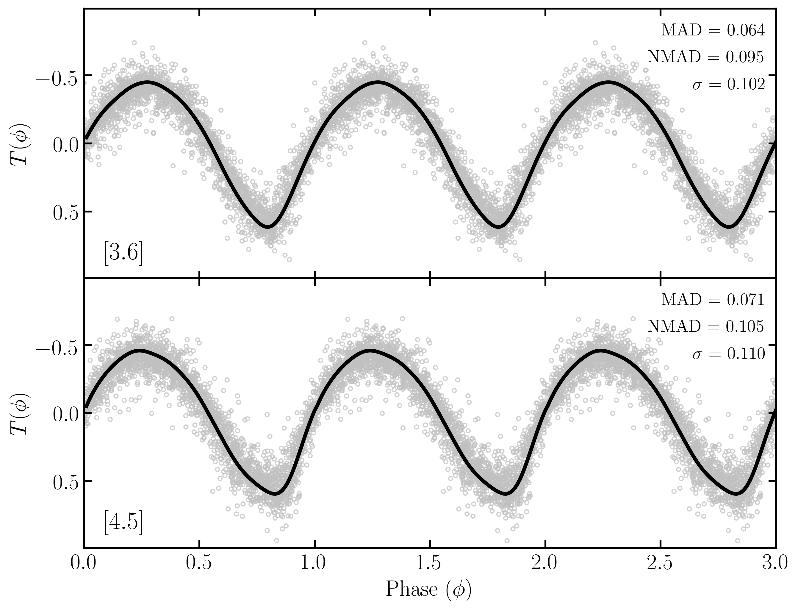
To quantify the optimal grouping method, we computed the median absolute deviation (MAD) between the observed value and the template value at . The MAD for each of the grouping methods is provided in Table 2. While the long period Cepheids with days have the smallest MAD value of 0.047 mag, we find that the MAD value monotonically increases as we move to shorter periods, with the shortest period group having a MAD of 0.133 mag. As observed in Figure 1, the majority of our Cepheids in the complete sample would be in this shortest period group. Thus, on average we find that there is not an overall improvement when grouping by period compared to host galaxy or wavelength. For our templates we decided to group our Cepheids by wavelength only as it had the smallest average MAD value across the four grouping methods. The addition of separating further by galaxy, period or colour (or a combination of these) did not improve the results. Our final template light curves are shown in Figure 3.
4.2 Cepheid optical-infrared parameter relations
Applying a template light curve to a sparse set of observations requires knowledge of the appropriate scale and shift factors for amplitude and phase, respectively, to best fit the observations. However, due to the limited number of SAGE observations, we cannot compute the amplitude and phase directly from the infrared data alone. Instead, we used our calibrating sample to establish relationships between the optical and mid-IR Cepheid parameters, which are then used to infer the mid-IR amplitude and phase of mean magnitude along the rising branch for the complete sample.
4.2.1 Optical data
To establish optical-infrared parameter relations, we obtained all available photometric data in the and bands from the OGLE-IV catalogue666http://ogledb.astrouw.edu.pl/~ogle/OCVS/ for Magellanic Clouds Cepheids. For some Cepheids, the photometric data from the OGLE-III catalogue (Udalski et al., 2008) was used as OGLE-IV measurements were not available. Table 3 shows the proportion of Cepheids with data from OGLE-IV and OGLE-III. The vast majority of Cepheids have OGLE-IV band photometry available ( and for the LMC and SMC, respectively), with only a small percentage of Cepheids ( and for the LMC and SMC, respectively) requiring the use of OGLE-III data. While all SMC Cepheids had photometric data in at least one of the two bands, no photometric data was available in either band for 13 LMC Cepheids. These Cepheids were identified to be the longest period, and hence brightest, Cepheids, which would cause the detector to saturate. For these Cepheids, the OGLE team used their Difference Image Analysis pipeline, which produces artificial objects in close vicinity to the Cepheid, in order to determine their magnitude (I. Soszyński, private communication).
Mean and band magnitudes and band amplitudes are already given in the OGLE-IV and OGLE-III catalogues, and were obtained by Fourier decomposition of the light curves. However, band amplitudes are not provided. As this parameter is required to derive our template fitting parameter relations, we decided to fit the data with GLOESS to determine its amplitude. In addition, since we use GLOESS fitting throughout this work, we chose to recompute the and magnitudes and band amplitudes using GLOESS, in order to maintain consistency within our work.
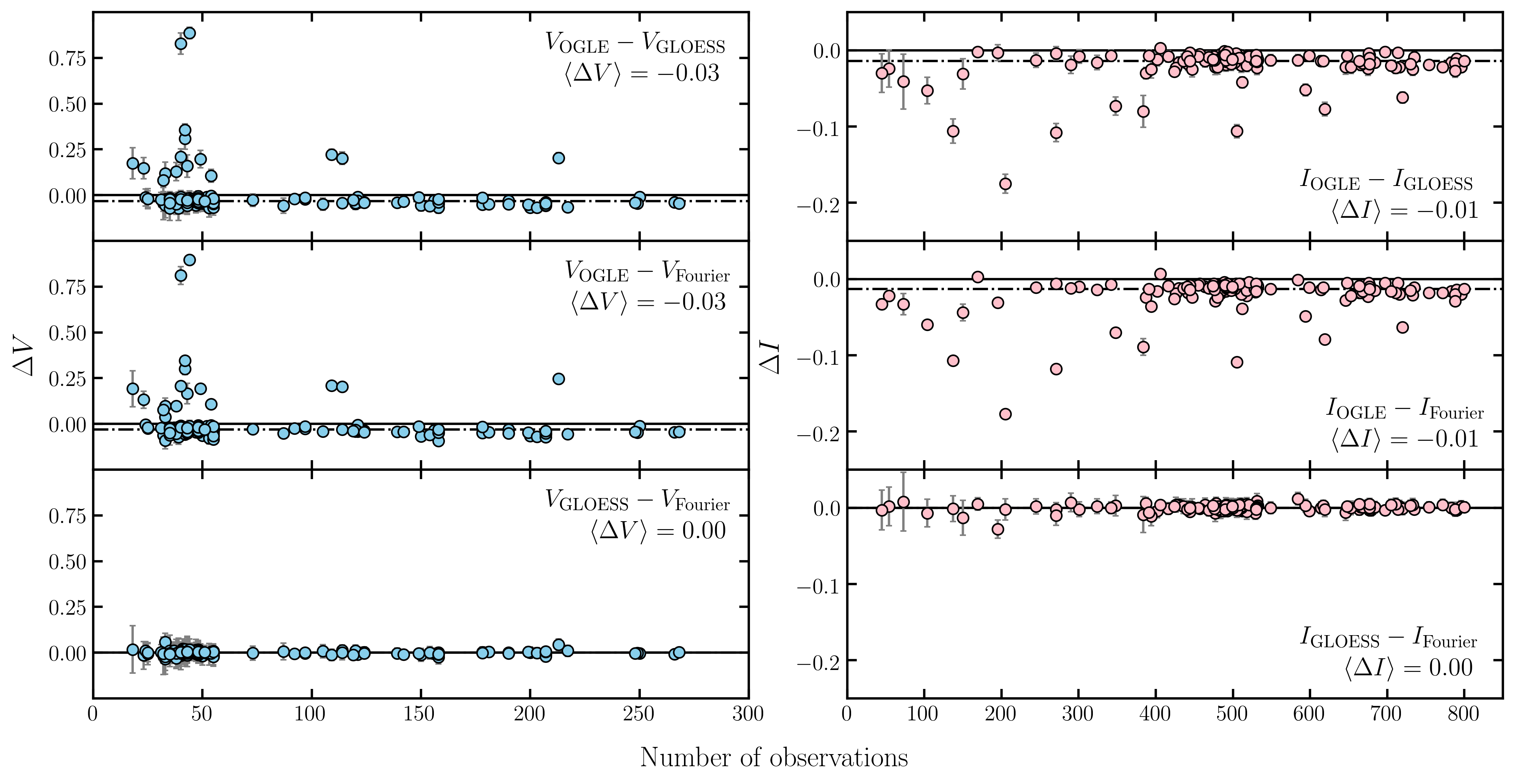
In the two top panels of Figure 4, we compare the mean magnitudes of our calibrating Cepheids computed by GLOESS fitting to those given in the OGLE-IV catalogue. In the band, we find a significant number of Cepheids with much brighter ( mag) GLOESS magnitudes than their OGLE-IV catalogue counterparts. For the most discrepant Cepheid HV00877 (OGLE-LMC-CEP-0461), the GLOESS and OGLE-IV catalogue magnitudes are 13.356 and 14.246 mag, respectively ( mag). Looking at the photometric data, we find that the magnitude given in the OGLE-IV catalogue is unfeasible, as the photometric data only range from mag. However, we find that the band magnitude given in the OGLE-III catalogue is 13.344 mag, which is consistent with our GLOESS magnitude ( mag). Aside from these Cepheids that have much brighter GLOESS magnitudes, all remaining Cepheids exhibit a systematic offset between the GLOESS and OGLE-IV magnitudes, with the OGLE-IV magnitudes being systematically brighter. This offset is also observed for the band.
While a detailed analysis of these OGLE discrepancies is beyond the scope of the paper, we briefly discuss Cepheids with mag and mag. of these Cepheids (7 out of 17) were discrepant in both and , have both and data but are only discrepant in one band, and the remaining have only single band data. Several of the discrepant Cepheids have a similar issue as HV00877, where the mean magnitude given in the OGLE-IV catalogue is outside the range of photometric measurements for that star. Some Cepheids have large amplitudes, in excess of one magnitude, such that their small discrepancies (of around 0.08 mag) are not as significant. Finally, several Cepheids have OGLE-IV mean magnitudes that are too bright or too faint, given the range of photometric measurements. For example, HV11211 has an OGLE-IV mean magnitude of 12.965 mag, which occurs right at the top of the light curve. At this time, we are unable to provide explanation for the cause of this discrepancy and further investigation is required.
In light of these magnitude discrepancies, we also fit the photometric data with a fourth order Fourier series of the form
| (4) |
where is the magnitude at time , is the mean magnitude, and and are the amplitude and phase parameters of the harmonic, respectively. The differences between our Fourier-derived mean magnitudes and those provided in the OGLE-IV catalogue, which also uses Fourier decomposition, are shown in the middle panels of Figure 4. Again, we find large discrepancies in mean magnitude for a substantial number of Cepheids, as well as a systematic offset for the remainder of the Cepheids. However, as shown in the bottom panels of Figure 4, we find the GLOESS mean magnitudes and those derived from our own application of Fourier decomposition are consistent.
| [3.6] | [4.5] | |||||
|---|---|---|---|---|---|---|
| 0.310 0.026 | 0.054 0.022 | 0.07 | 0.334 0.025 | 0.023 0.022 | 0.07 | |
| 0.461 0.049 | 0.077 0.025 | 0.07 | 0.493 0.046 | 0.047 0.024 | 0.07 | |
As a result of the above analysis, we decided to use the mean magnitudes computed by GLOESS fitting. We chose to do this for a number of reasons. First, there are unexplained discrepancies between OGLE-III and OGLE-IV magnitudes for the same Cepheid. Second, we have verified that our GLOESS magnitudes are consistent with the magnitudes obtained through our own Fourier decomposition. Finally, to avoid introducing any possible systematic, we fit the optical data using GLOESS as our photometry pipeline fits the mid-IR data with GLOESS.
In the remainder of this work, any optical parameters used will be the GLOESS-derived values as opposed to the values provided in the OGLE catalogues. However, we do continue to use the periods from OGLE, as these are extremely accurate, with uncertainties on the order of s.
4.2.2 Optical-infrared amplitude relation
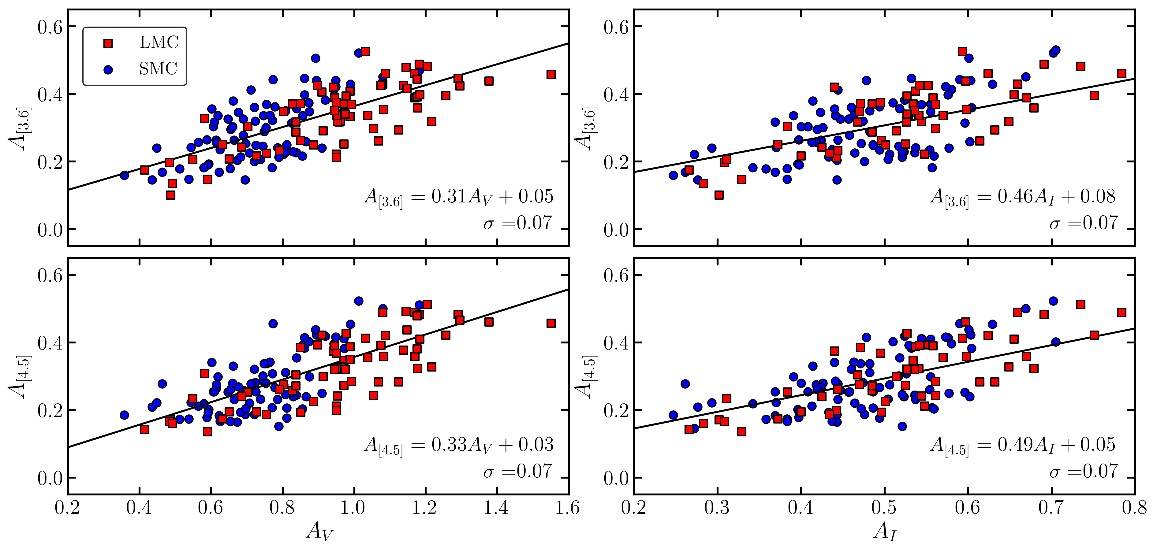
In order to fit a template to sparse data, we must be able to scale our template by the appropriate amplitude that best fits the available observations. In Figure 5, we show the relationship between Cepheid amplitudes in the various optical and mid-IR photometric bands; we find a positive () correlation in each case. For each combination of bands, we performed an unweighted linear least squares fit, with the derived parameters and their uncertainties provided in Table 4. We find a dispersion of 0.07 mag for all relations. These relations allow us to estimate the mid-IR amplitude of a Cepheid based solely on its optical amplitude.
4.2.3 Optical-infrared phase relation
In addition to the amplitude, we must also know the phase at which the mean magnitude occurs along the rising branch, denoted , for the mid-IR light curve. To this end, we define the phase lag as the difference in between the mid-IR and optical light curves of a Cepheid, given by
| (5) |
where is either or and is either or .
| 0.15 | 0.04 | 0.13 | 0.05 | |
| 0.12 | 0.05 | 0.09 | 0.05 | |
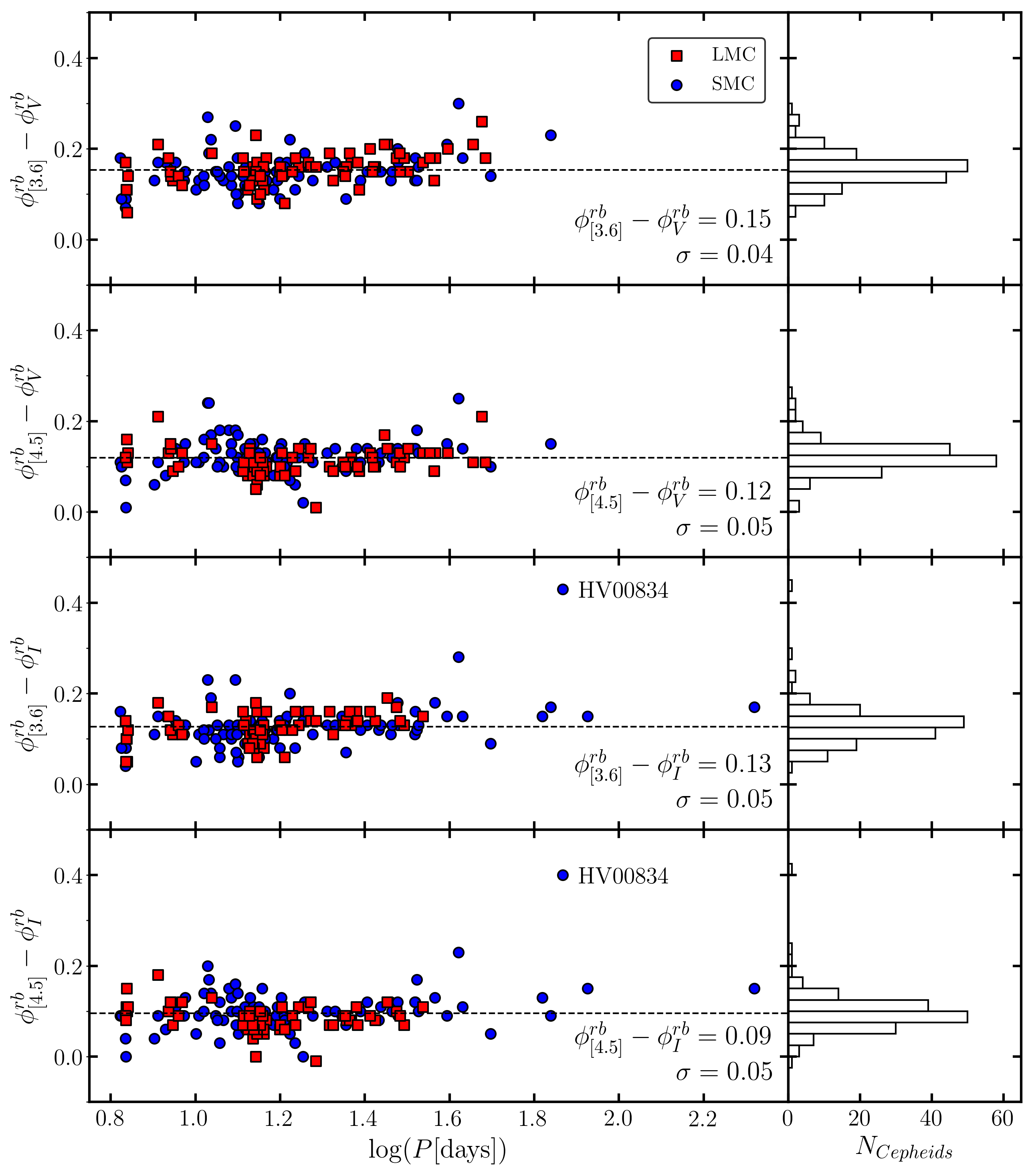
In Figure 6, we present the phase lags as a function of period for each optical and mid-IR band combination. We find that, with the exception of HV00834 which is highlighted in the bottom two panels of the Figure, the majority of the phase lags fall around a similar value, with the mean phase lag and dispersion for each combination of bands provided in Table 5. These mean values are shown by the dashed line in each of the panels.
We checked whether there was any dependence of the phase lags on pulsation period. We fit a linear relation of the form to the phase lags and found that for all band combinations the slope, , was consistent with zero, verifying that there is no significant dependence on period. Similarly, we found no significant dependence on the host galaxy so the LMC (red squares) and SMC (blue circles) samples were combined.
While HV00834 band photometry is not available, the band phase lags are discrepant from the general trend. Looking at the band light curve for this Cepheid, we found the observations to be very noisy, making it difficult to determine a reliable determination of . However, band photometry is also available from Moffett et al. (1998)777The ID for HV00834 is incorrectly identified as HV00824 in the Moffett et al. (1998) Vizier catalogue.. When using these data, we find and , which makes HV00834 consistent with the rest of the sample.
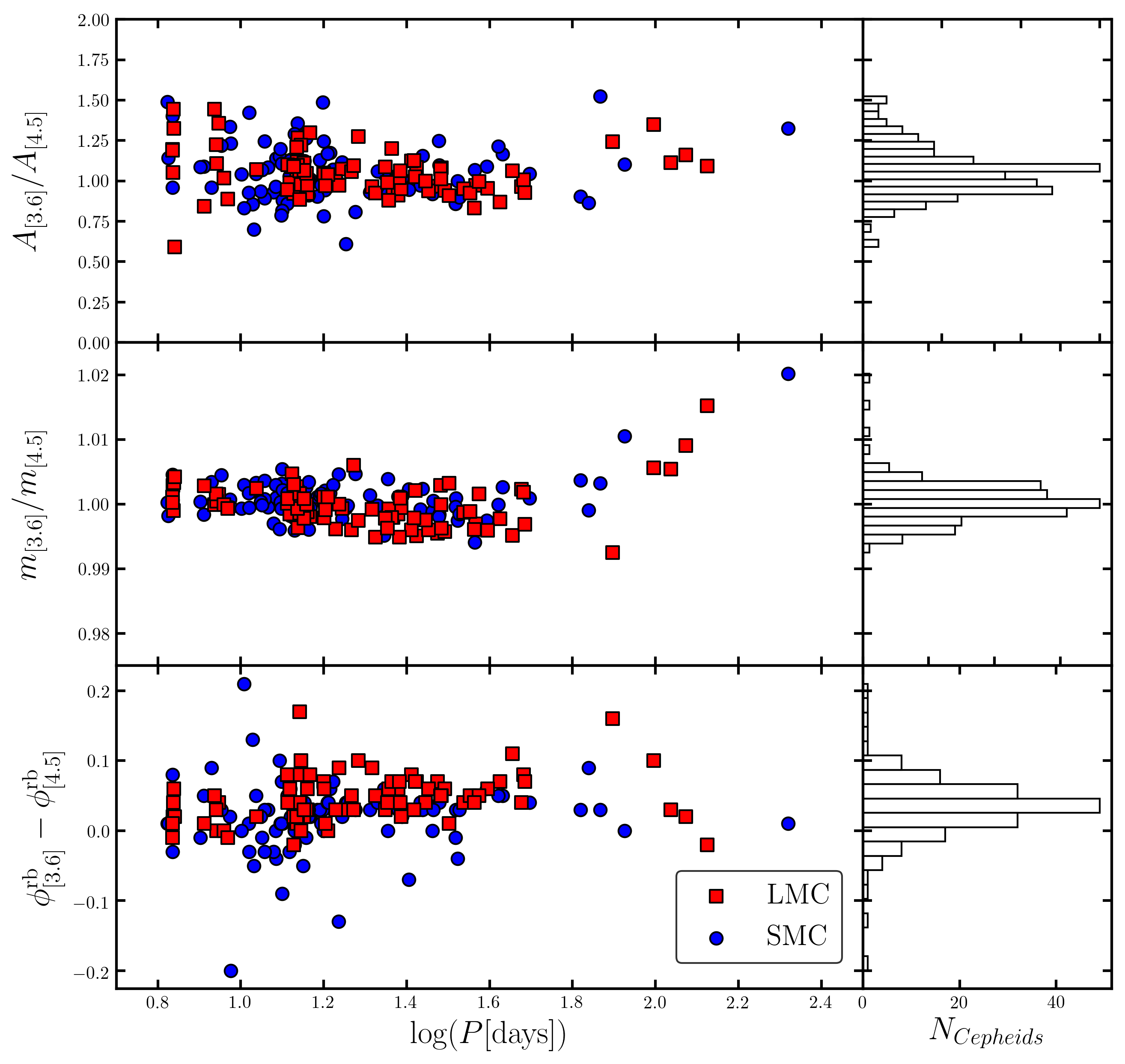
To summarise, the relations given by Tables 4 and 5 allow us to estimate the mid-IR amplitude and phase of mean magnitude along the rising branch for a Cepheid, based solely on its optical data. Thus, we can use these relations to scale our normalised template light curves to the sparsely-sampled SAGE data to compute the mean magnitude for each Cepheid in our complete sample.
4.3 Template fitting method
Now that we have created our templates and can scale and shift them in amplitude and phase, we outline the process of fitting the templates to data. Rather than assuming the infrared amplitude and phase inferred using the results of the previous section to be undoubtedly true, we instead use these values as initial starting guesses and employ Markov Chain Monte Carlo (MCMC) methods via the emcee Python package (Foreman-Mackey et al., 2013) to find the optimal value of each parameter. The parameters to be determined for each Cepheid are , resulting in a six-dimensional parameter space. Each Cepheid has a set of observations, .
As the template light curve is scaled by the optimal amplitude, shifted in phase by the optimal and then shifted in magnitude by the optimal magnitude, it is necessarily the case that this optimal magnitude lies exactly halfway between maximum and minimum light. Therefore, instead of taking this optimal magnitude as our final value, we use the final fitted light curve to compute the intensity-averaged mean magnitude.
We explored the parameter space using 50 walkers, with each walker performing 1000 burn-in steps followed by a further 10,000 steps. The initial starting amplitude and phase of the walkers are given by the relations provided in Tables 4 and 5, and an initial magnitude in each band is computed as the average of the available observations. If both and band data are available, then we prefer to use the band values to compute the initial parameter estimates, as these were derived from many more observations than the band (as shown in Figure 4). If band data are unavailable, then we use the band data. For the 13 LMC Cepheids with no available optical data, we set the initial amplitude to be the average band amplitude of the complete sample ( mag) and we set the initial phase to be .
We impose a series of Gaussian and uniform priors on our parameters. The mid-IR amplitudes follow a Gaussian prior, centered on the initial estimate from Table 4 with given by the corresponding scatter on the relation. The mid-IR phase follow a Gaussian prior centered on the initial estimate from Table 5 with the corresponding . The mid-IR mean magnitudes follow a Gaussian prior centered on an initial mean magnitude given by the average of the available observations, with mag chosen as this is the intrinsic width of the instability strip in the mid-IR. We also impose restrictions on the amplitude ratio, phase difference and magnitude ratio between the and bands, adopting uniform priors such that , and . The justification for these priors is given in Appendix B.
For each MCMC step, we have a trial combination of our parameters () for each mid-IR band, which are used to scale the appropriate template light curve. For the likelihood function, we use the standard -squared minimisation to determine how well the scaled template and thus the current trial parameters fit to the observed data.
| LMC | 1 | 0.048 | 0.040 | 0.102 | 0.064 |
|---|---|---|---|---|---|
| 2 | 0.023 | 0.018 | 0.073 | 0.060 | |
| 3 | 0.020 | 0.016 | 0.053 | 0.042 | |
| 4 | 0.018 | 0.017 | 0.046 | 0.035 | |
| 5 | 0.014 | 0.012 | 0.042 | 0.030 | |
| 6 | 0.011 | 0.009 | 0.030 | 0.026 | |
| 1 | 0.042 | 0.031 | 0.106 | 0.061 | |
| 2 | 0.025 | 0.021 | 0.068 | 0.061 | |
| 3 | 0.022 | 0.018 | 0.051 | 0.039 | |
| 4 | 0.018 | 0.015 | 0.042 | 0.034 | |
| 5 | 0.012 | 0.009 | 0.041 | 0.031 | |
| 6 | 0.011 | 0.009 | 0.033 | 0.028 | |
| SMC | 1 | 0.046 | 0.034 | 0.091 | 0.058 |
| 2 | 0.029 | 0.021 | 0.062 | 0.050 | |
| 3 | 0.023 | 0.021 | 0.049 | 0.038 | |
| 4 | 0.014 | 0.012 | 0.043 | 0.034 | |
| 5 | 0.013 | 0.011 | 0.037 | 0.026 | |
| 6 | 0.011 | 0.009 | 0.028 | 0.023 | |
| 1 | 0.043 | 0.034 | 0.080 | 0.055 | |
| 2 | 0.026 | 0.023 | 0.060 | 0.048 | |
| 3 | 0.020 | 0.017 | 0.049 | 0.034 | |
| 4 | 0.016 | 0.011 | 0.040 | 0.035 | |
| 5 | 0.013 | 0.011 | 0.033 | 0.024 | |
| 6 | 0.011 | 0.010 | 0.028 | 0.022 |
4.4 Validation of template fitting method
To assess the accuracy of our template fitting method, we used the observations of the calibrating sample to simulate a mock dataset that mimics typical SAGE data. As each Cepheid in the complete sample has a maximum of six observation epochs, we randomly selected between one and six observations for each of our calibrating Cepheids, which serves as their sparse set of observations. We allowed observations to be selected multiple times, as it is likely that the SAGE observations will overlap in phase in some cases since the observations were not designed to be equally-spaced. While this test is not truly independent, as we are using the same data for both the validation of the method and the creation of the method itself, we see from the dispersion of our template fitting parameter relations in Tables 4 and 5 that just using the mid-IR value inferred from a relation will not guarantee the optimal result. Therefore, this test does provide insight into the code’s ability to find the best-fitting amplitude, phase and mean magnitude in each band.
The template fitting code was run on this mock dataset for each calibrating Cepheid in the LMC and SMC and at both mid-IR wavelengths. Examples of the fitted mid-IR light curves are shown in Figure 7. The observations used in the template fitting are given by the yellow and red points for the and band, respectively, while the grey points are the observations not used. The black solid lines are the “true” mean magnitudes obtained from GLOESS fitting to all available observations while the dashed-dot line shows the template-derived mean magnitude using the available observations, showing the excellent agreement between the two methods.
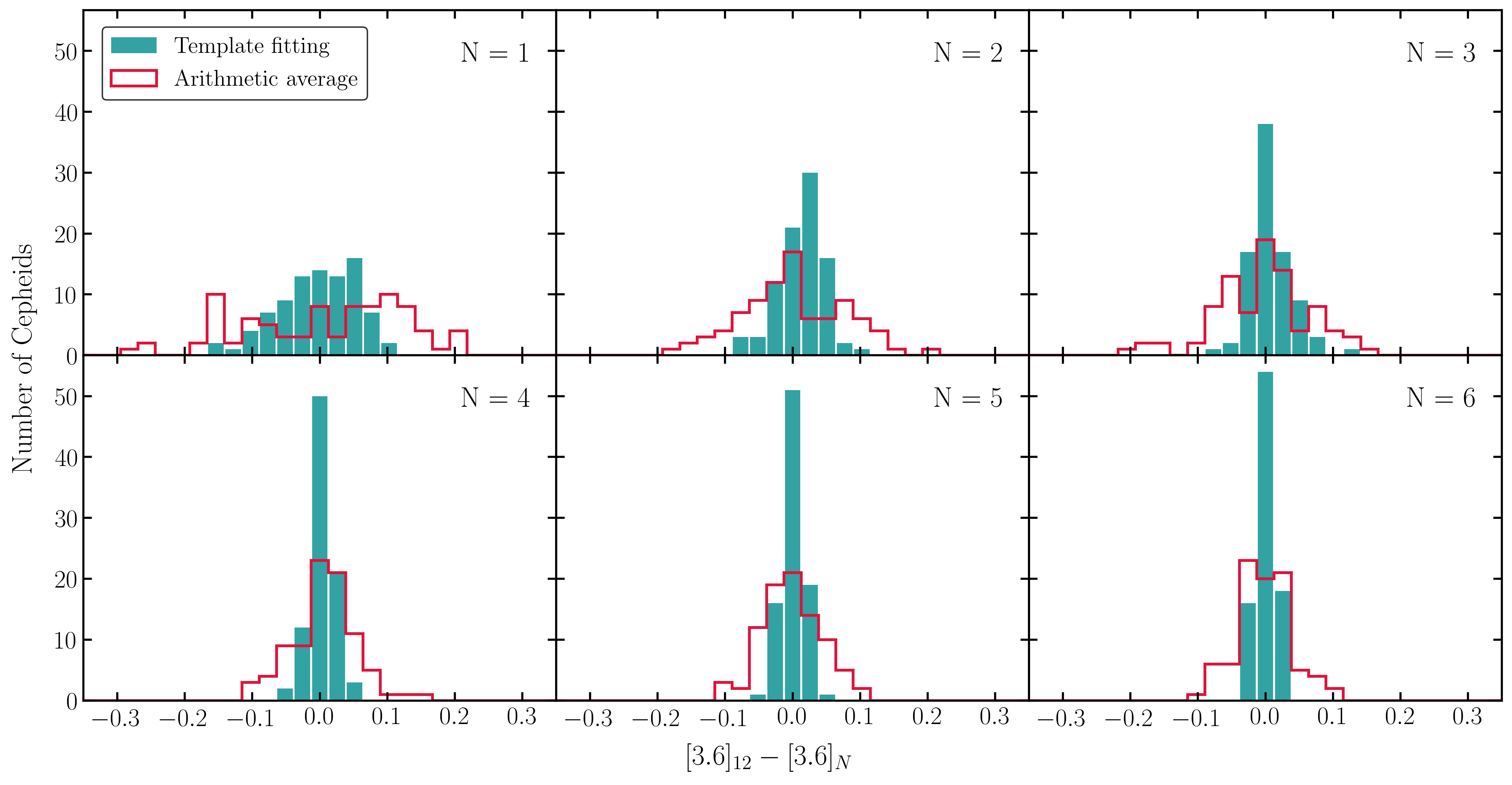
For each galaxy and wavelength, we computed the mean absolute difference between the template-derived magnitudes, , for observations and those obtained through GLOESS fitting to 12 or 24 equally-spaced observations. The results of this test are provided in Table 6. An example of these results is shown by the blue filled distributions in Figure 8 for the SMC band. These results show that our template fitting method produces mean magnitudes that are in good agreement with the “true” values obtained through 12 fully-phased observations and GLOESS fitting, with a precision that increases with the number of observations. For a single observation of an SMC Cepheid, the mean absolute difference was mag, reducing to mag for six observations. For three phase points, which is the most common number of observations for the SAGE data, the mean absolute difference was 0.02 mag.
It is also important to verify that our template fitting procedure provides more accurate mean magnitudes than just taking the arithmetic mean of the observations. The red, non-filled distributions in Figure 8 show the differences between GLOESS fitting to 12 fully-phased observations and those obtained from simply averaging the magnitudes. Comparing these distributions from the template fitting procedure clearly demonstrates the significant improvements provided by our technique. We observe that the template-fitted distributions are more concentrated around , having significantly smaller dispersions than the arithemtic estimates. Thus, mean magnitudes derived from our template fitting method will be more precise than just taking the average of the available observations.
We conclude that our template fitting procedure is a suitable method for obtaining mid-IR mean magnitudes for Cepheids with few, sparse observations. We find that the fitting is more precise if the chosen observations provide good coverage of the entire pulsation cycle. However, we lose precision if the available observations are too close in phase, due to the fact that some observations become redundant. These redundant observations do not provide the fit with any additional information about the light curve as they are situated in the same region of the pulsation cycle as the other observations. These results populate the tails of the template-fitted distributions of Figure 8.
| Galaxy | OGLE ID | Period (d)a | b | b | c | Rejected?d |
|---|---|---|---|---|---|---|
| LMC | OGLE-LMC-CEP-0002 | 3.118 | 14.833 0.017 | 14.670 0.049 | 0.080 0.017 | N |
| LMC | OGLE-LMC-CEP-0005 | 5.612 | 13.709 0.031 | 13.624 0.049 | 0.074 0.015 | N |
| LMC | OGLE-LMC-CEP-0016 | 10.564 | 12.332 0.032 | 12.314 0.042 | 0.296 0.004 | N |
| LMC | OGLE-LMC-CEP-0017 | 3.677 | 14.289 0.054 | 14.199 0.054 | 0.076 0.012 | N |
| LMC | OGLE-LMC-CEP-0018 | 4.048 | 14.258 0.026 | 14.173 0.044 | 0.107 0.024 | N |
| … | … | … | … | … | … | … |
| SMC | OGLE-SMC-CEP-4976 | 36.737 | 11.347 0.011 | 11.361 0.010 | 0.000 0.000 | N |
-
(This table is available in its entirety at https://doi.org/10.15125/BATH-00915.)
- Notes:
- a
Periods were taken from the OGLE-IV catalogue (http://ogledb.astrouw.edu.pl/~ogle/OCVS/) b and are the intensity-averaged mean magnitudes in each mid-IR band and have not been corrected for reddening. c Colour excess values computed from the application of the Cardelli et al. (1989) and Indebetouw et al. (2005) reddening laws, assuming . d Flags whether a Cepheid is rejected from further analysis due to poor SAGE data.
5 Results
Our template fitting method was performed on the SAGE photometric data for the complete sample of Cepheids. As the calibrating and complete samples overlap, we decided to incorporate the CHP observations for the calibrating sample into the template fitting for these Cepheids in order to utilise the vast number of observations available. Since the SAGE footprint does not cover as large an area as the OGLE footprint, a small percentage of the complete sample were observed in the optical bands but not in the mid-IR. We discarded from our sample the 125 LMC and 82 SMC Cepheids that did not have both and magnitudes. Our final complete sample contains 2352 LMC and 2672 SMC Cepheids.
5.1 Mid-infrared Cepheid light curves
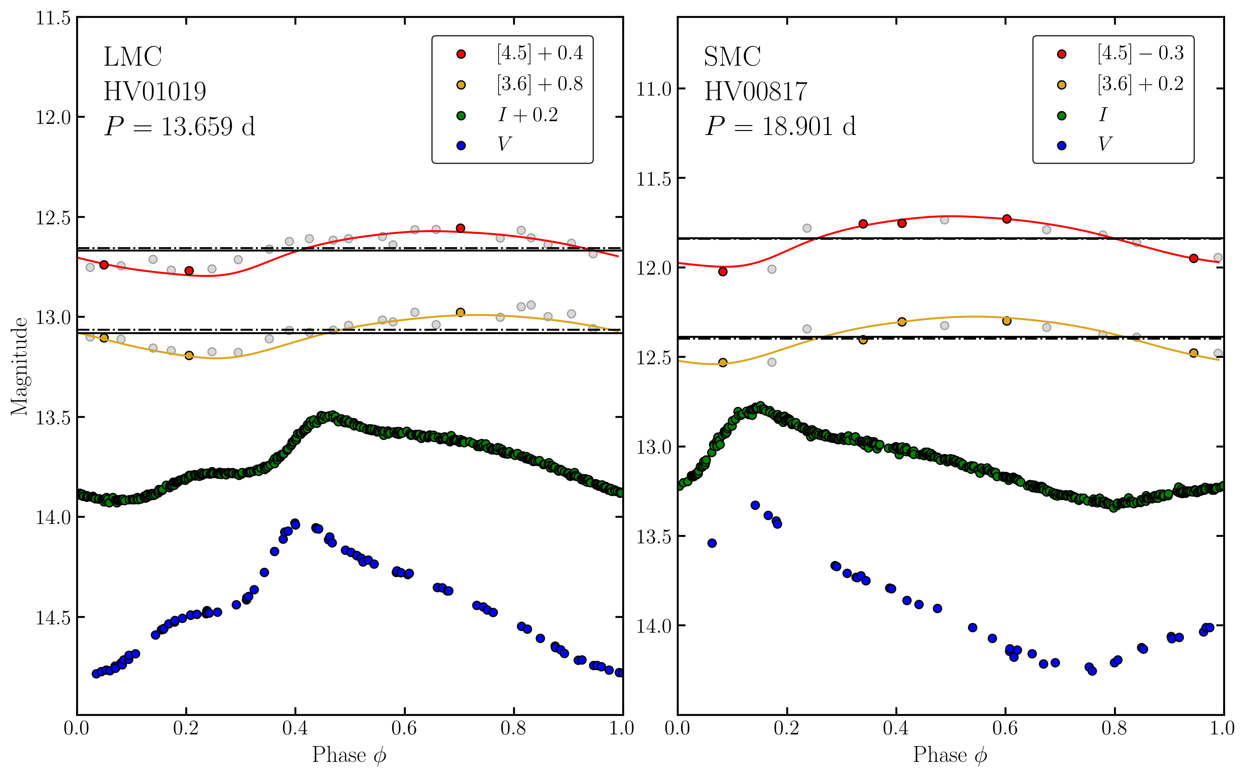
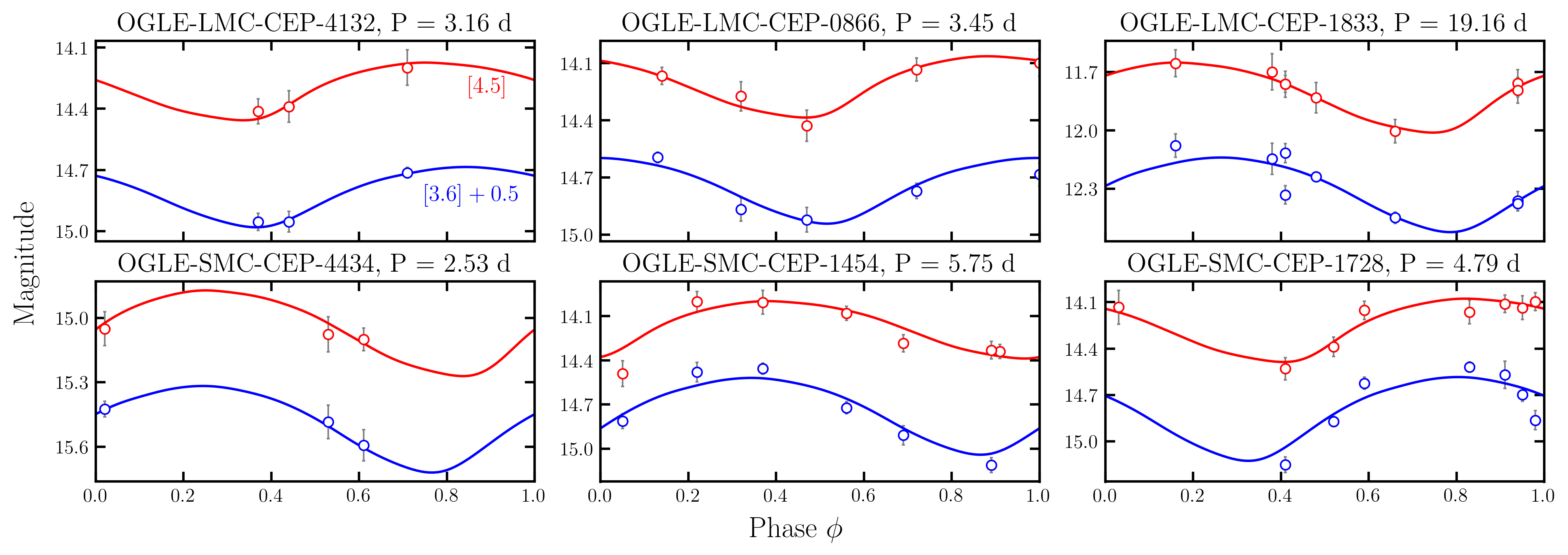
In Figure 9, we show a selection of Cepheid light curves fit using our template fitting procedure for different numbers of observations. Each plot shows both the (blue) and (red) fitted light curves, along with the available photometric observations used to fit the template. The top panels show examples from the LMC, while the bottom panels show light curves for a selection of SMC Cepheids. As can be seen from Figure 9, our templates fit the available observations well.
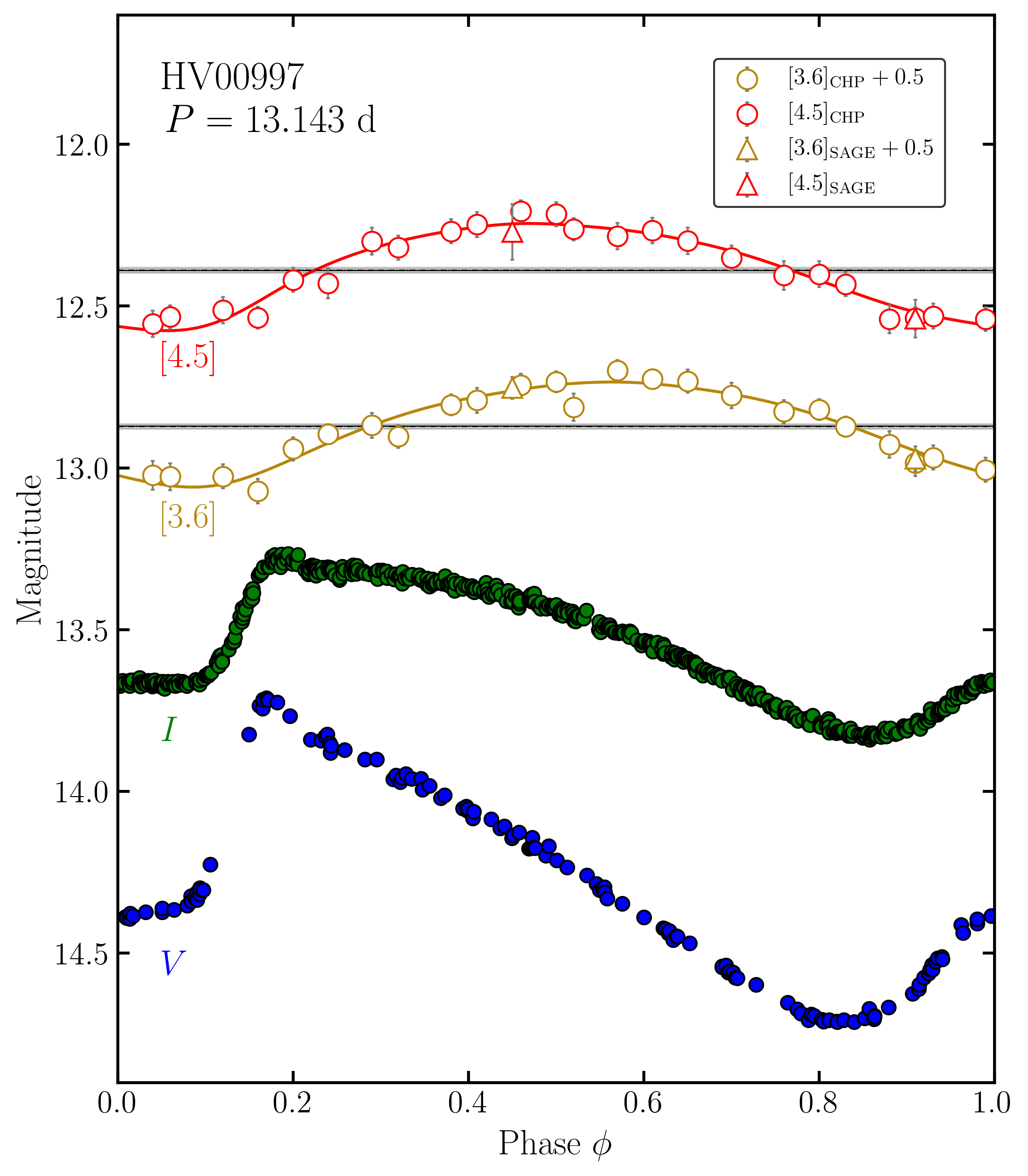
In Figure 10, we show the mid-IR and optical light curves for the LMC calibrating Cepheid HV00997. This Cepheid had mid-IR observations from both CHP and SAGE, and we incorporated all available observations into the template fitting procedure. Figure 10 demonstrates the good agreement between the two photometry pipelines, as the additional SAGE observations (triangles) are consistent with the CHP observations (circles).
5.2 Mid-infrared mean magnitudes for Cepheids in the Magellanic Clouds
Table 7 provides our mid-IR catalogue of fundamental mode Classical Cepheids. The colour excess for each Cepheid was computed as described in Section 5.2.1 and is given in the final column. As described in Section 5.2.2, we removed a subset of our sample due to their poor mid-IR data. In doing so, our catalogue provides the mid-IR mean magnitudes for 2311 LMC and 2637 SMC Cepheids. The mean and magnitudes and associated uncertainties were computed from the application of our MCMC template fitting procedure described in Section 4.3. The magnitudes provided in Table 7 have not been corrected for reddening but can be corrected using and Equations 6 and 7. The average uncertainty on the mean magnitude for the LMC Cepheids is and mag in the and , respectively. For the SMC, the average and uncertainties are and mag, respectively. The periods given here are taken from the OGLE-IV catalogue and have uncertainties on the order of s.
5.2.1 Reddening correction
Although we are working at mid-IR wavelengths, where extinction is greatly reduced compared to optical wavelengths, we must still apply a reddening correction to our mid-IR magnitudes. While these corrections are small, they are a necessary step for ensuring precise mean magnitudes. To compute the size of the reddening correction for each Cepheid, we use one of two methods: application of the reddening law to multi-band photometry, or a nearest neighbours approach. The method used depends on whether OGLE-IV and band photometry is available for the Cepheid in question.
For the vast majority of Cepheids ( and for the LMC and SMC, respectively), we computed the reddening value by fitting appropriate reddening laws to multi-band photometry. We did not use the magnitude in this fit, as this band is known to be affected by the CO band-head (Scowcroft et al., 2016a). We fit the reddening laws of Cardelli et al. (1989) and Indebetouw et al. (2005) to the , and magnitudes of each Cepheid by minimising the dispersion of the distance moduli around the values predicted by the reddening law. The distance modulus in each of the three bands was computed by adopting literature LLs as fiducial. For the and band, we used the relations given in Fouqué et al. (2007), while for the band we used the relation given in Monson et al. (2012).
For the remaining Cepheids that did not have , and magnitudes available, we computed the reddening as the average reddening value of the star’s nearest neighbours. We set the search radius to be deg and deg for the LMC and SMC, respectively. These values were chosen as, when creating reddening maps for the LMC and SMC using OGLE-IV Cepheids, Joshi & Panchal (2019) divided each galaxy into segments with a mean spatial resolution of deg2 and deg2, respectively. The SMC was divided into smaller segments than the LMC as it contains a higher density of Cepheids in a smaller region of the sky.
The colour excess for each Cepheid is given in the final column of Table 7. The mean magnitudes provided in Table 7 have not been corrected for reddening. Reddening-corrected mid-IR mean magnitudes are computed using the extinction equations given in Monson et al. (2012),
| (6) | |||
| (7) |
5.2.2 Bad data rejection
To clean our data, we performed a preliminary unweighted least-squares fit of the LL to the dereddened magnitudes
| (8) |
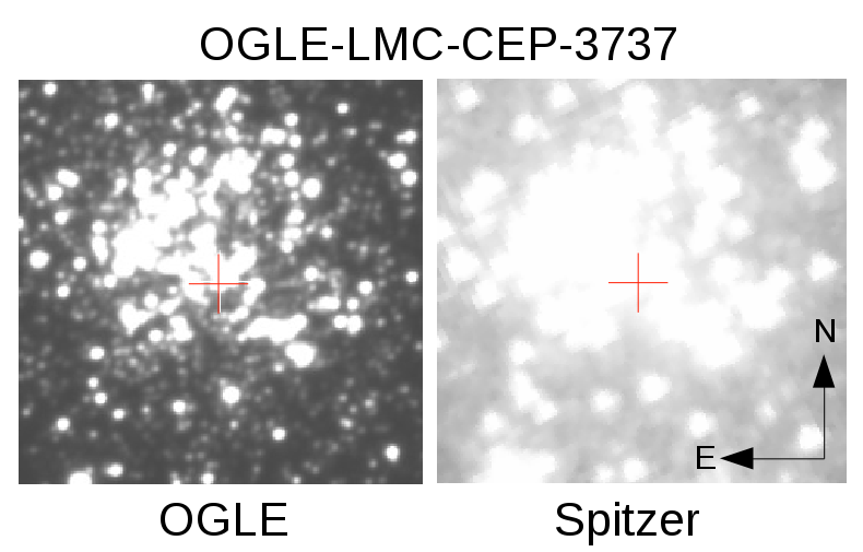
where the term is preferred over just a term as it reduces the correlation between the slope and the intercept. This fit was carried out for both galaxies and at both mid-IR wavelengths. We performed a visual inspection of the original images for stars which lay more than from the LL to check for potential contamination. In all cases, these Cepheids were either blended with a nearby companion or were part of a large unresolved ‘blob’ of stars causing erroneously bright magnitude measurements. Figure 11 shows an example of this effect for the LMC Cepheid OGLE-LMC-CEP-3737. As a result, we removed all Cepheids with such an effect in either of the two bands. In total, 41 LMC and 35 SMC Cepheids were discarded, resulting in a cleaned sample of 2311 LMC and 2637 SMC Cepheids.
5.3 The mid-infrared Leavitt Law for the Magellanic Clouds
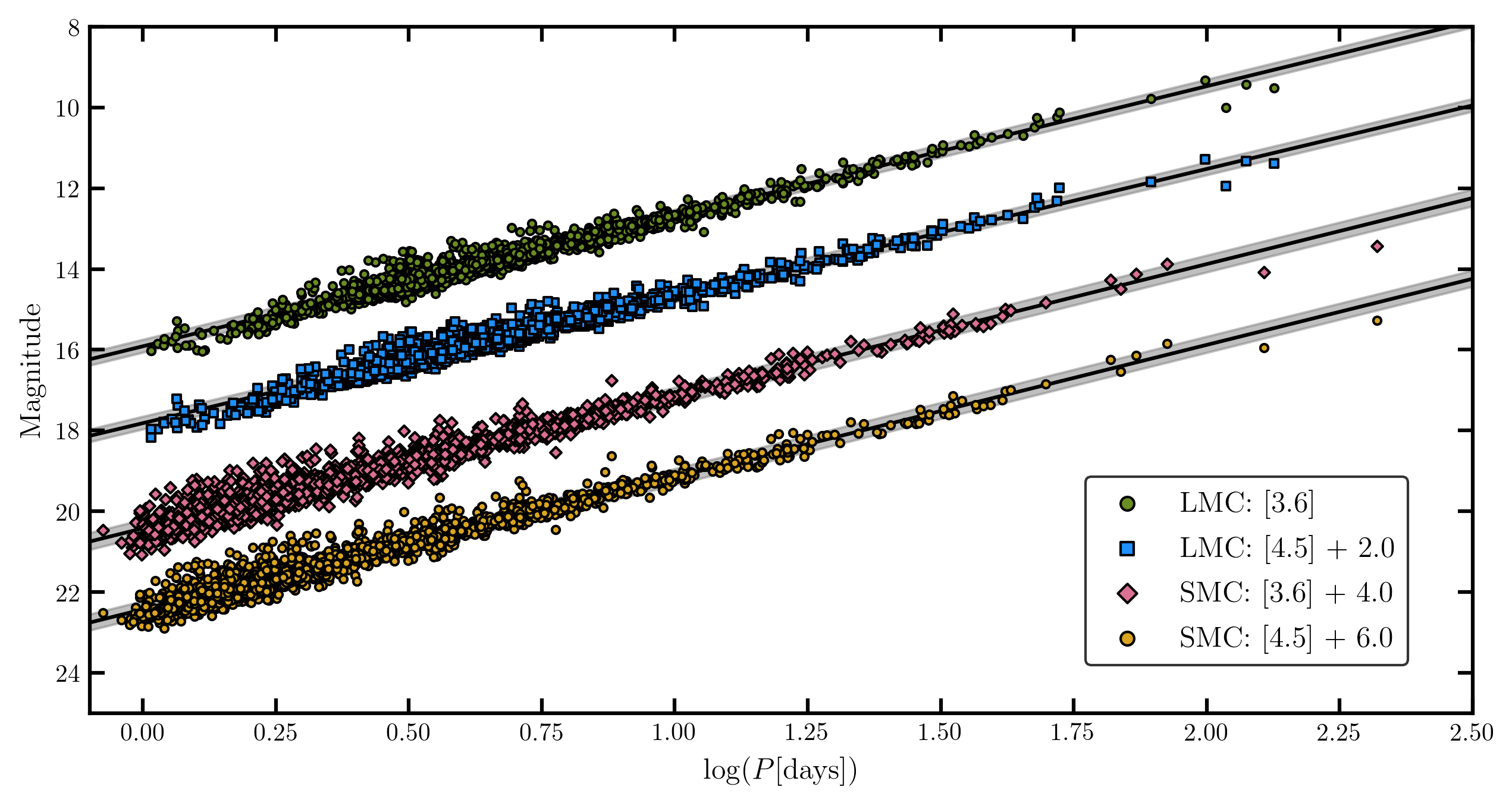
Using our mid-IR catalogue in Table 7, we show the dereddened and LLs for the LMC and SMC in Figure 12. We perform a standard inverse-variance weighted least squares fit of the form given in Equation 8 for both bands and both galaxies. Table 8 gives the slope and intercept values, their associated uncertainties, and the standard deviation of the fit. We stress that the slope and zero point values given here are not our final values. We devote the entirety of Section 6.1 to investigating the dependence of the LL coefficients on various characteristics of the sample. Our final adopted fits and their zero point calibration are given in Section 6.3.
6 Discussion
6.1 Dependence of the Leavitt Law on sample characteristics
| Galaxy | Wavelength | Period Range | ||||
|---|---|---|---|---|---|---|
| LMC | No cuta | 0.156 | 2311 | |||
| 0.137 | 420 | |||||
| b | 0.107 | 80 | ||||
| 0.155 | 2099 | |||||
| 0.156 | 2290 | |||||
| No cuta | 0.158 | 2310 | ||||
| 0.136 | 420 | |||||
| b | 0.116 | 80 | ||||
| 0.154 | 2099 | |||||
| 0.157 | 2290 | |||||
| SMC | No cuta | 0.198 | 2637 | |||
| 0.146 | 267 | |||||
| b | 0.147 | 85 | ||||
| 0.221 | 1644 | |||||
| 0.174 | 993 | |||||
| No cuta | 0.207 | 2637 | ||||
| 0.150 | 267 | |||||
| b | 0.150 | 85 | ||||
| 0.220 | 1644 | |||||
| 0.171 | 993 |
-
Notes:
-
a These fits are given by the solid lines in Figure 12.
-
b These fits used only the calibrating sample which have fully-phased observations of their light curve.
The large number of Cepheids in our sample allows for the exploration of selection effects on the LL coefficients. Rather than showing here the analysis for both the LMC and SMC at both and bands, we choose to focus our attention on the LMC relation, as it is the relation that is primarily used for distance measurements. We investigate the dependence of the LL coefficients on the number of observations for each Cepheid, the mean magnitude uncertainties for each Cepheid, the period distribution of the sample, and whether or not the relation is more appropriately described by a non-linear relation.
6.1.1 Slope and zero point dependence on the number of observations
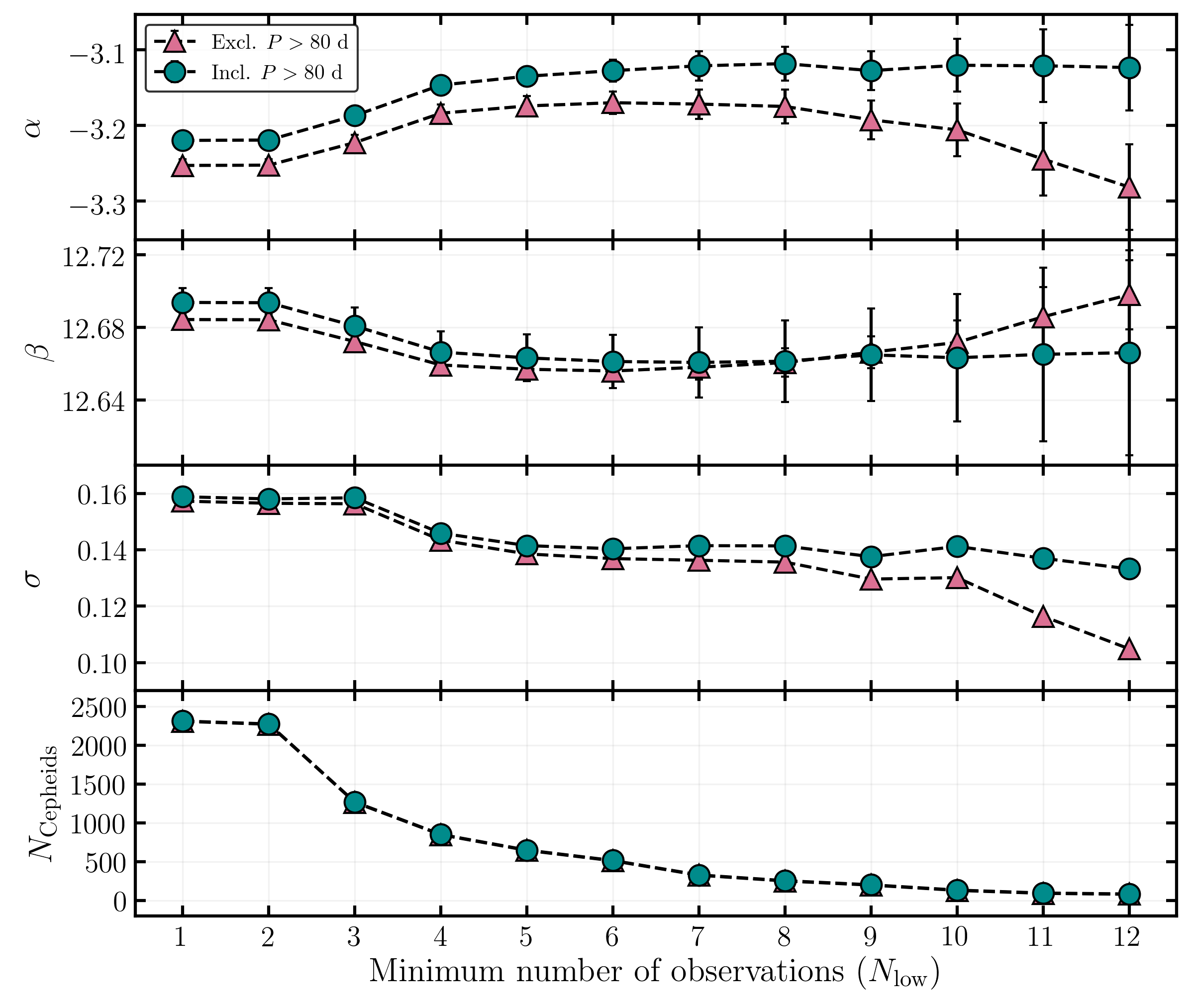
Cepheids with a larger number of observations carry smaller uncertainties on their mean magnitude, such that . Therefore, we tested what effect requiring a minimum number of observations has on the coefficients of the LL. As observed in Figure 12, there are four ultra-long period (ULP) Cepheids in the LMC sample, all of which are in our calibrating sample and have fully-phased observations. ULP Cepheids have periods greater than 80 days (Bird et al., 2009). Cepheids with such long periods are often excluded from analysis of the LL as there is evidence that they obey their own LL (Bird et al. 2009; Fiorentino et al. 2012). Therefore, we performed our analysis twice: once including the ULP Cepheids and once excluding them, shown by the blue and pink points in Figure 13, respectively. We applied a minimum number of observations criteria for our sample, from observations. Cepheids that do not meet this criteria were discarded and a weighted linear least squares fit of the LL was performed on the remaining Cepheids.
The slope of the LLs when including and excluding the ULP Cepheids are qualitatively similar up to , as they follow the same shape but with systematically steeper slopes when excluding the ULP Cepheids. For , there are substantially fewer Cepheids remaining in the fit, resulting in the ULP Cepheids having more weighting in these fits and causing the slope to remain shallower. All of the ULP Cepheids were observed by the CHP and therefore have . Therefore, these Cepheids will never be knocked out for having too few observations and will have more weighting as increases and more Cepheids are removed. Without these Cepheids, we find that the slope becomes steeper as the minimum number of observations increases above 10. In both cases, the slope values are consistent for , possibly suggesting that imposing a requirement of at least four observations is optimal. The same result is found for the zero point , with consistent values for .
For increasing , the dispersion of the LL reduces, particularly when the ULP Cepheids are excluded. However, this improved dispersion must be counterbalanced by the fact that imposing this minimum observation criteria vastly reduces the number of Cepheids being used in the fit. For example, while the dispersion reduces from 0.157 to 0.143 mag for , the number of Cepheids reduces to only of the original sample (). We conclude that this improvement is not significant enough to warrant excluding the majority of our sample from the LL fit. While we do find significant improvements for , only of the Cepheids remain, resulting in a LL that is not representative of the entire Cepheid population.
6.1.2 Slope and zero point dependence on the period range
When determining the Cepheid LL, period cuts are often applied to remove potentially contaminating Cepheids. For example, Ngeow & Kanbur (2008) obtained the LMC mid-IR LLs by removing all Cepheids from their sample with days in order to avoid potential contamination by overtone Cepheids. S11 applied a similar short-period cut for their LMC LL by excluding Cepheids with days, in addition to a long-period cut at days as these Cepheids are known to deviate significantly from the LL. We now focus on how the LL coefficients are affected by employing these period cuts.
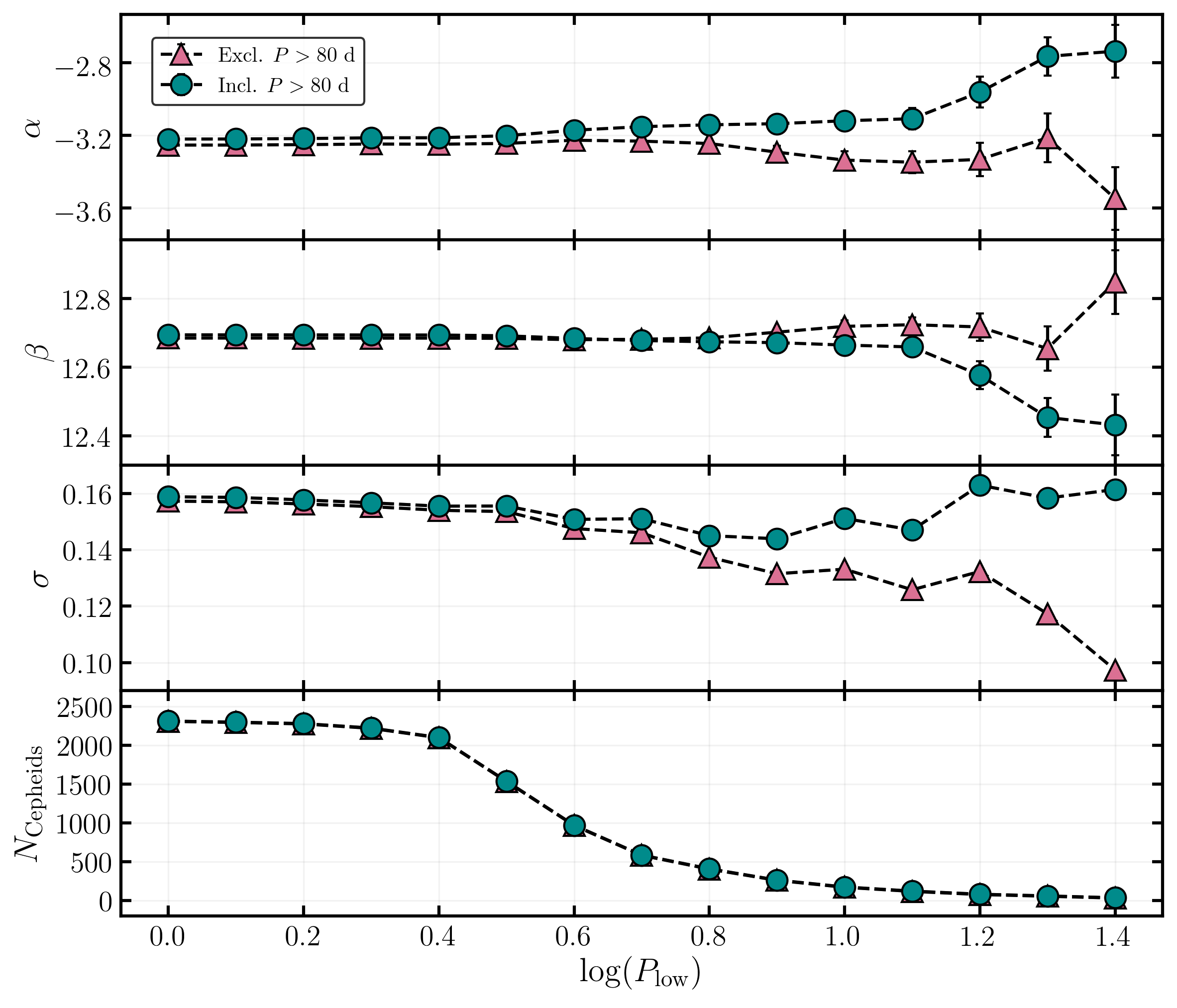
For each low cut-off value , we discard all Cepheids with and fit a weighted least squares LL of the form given in Equation 8. We test period cut values from in steps. Similarly to the previous sections, we perform two fits for each value of to include and exclude the ULP Cepheids. In Figure 14, we present the LL coefficients as function of . The top two panels show the slope and zero point , while the bottom two panels show the corresponding dispersion and number of Cepheids remaining in the sample . In each panel, the blue points show the results when including the ULP Cepheids and the pink points show the results when excluding them.
Regardless of whether we include the long period Cepheids, we observe consistent slope and zero point values (within ) up to a low cut off value of , corresponding to days. However, above this value we find that the inclusion of the ULP Cepheids results in a monotonic decrease in the slope and zero point, causing the values to be inconsistent. In contrast, excluding the ULP Cepheids results in a larger proportion of consistent values, with only and 1.4 not being in agreement within . As the low cut off value becomes larger, fewer Cepheids are included in the fit, resulting in the four ULP Cepheids having more leverage on the LL coefficients than when many more Cepheids are included. This is likely the reason why the coefficients are much more consistent when excluding these Cepheids. Moreover, for larger cut off values, the derived coefficients carry larger uncertainties due to the relatively smaller sample size.
In addition to applying a period cut at 2.5 days, Ngeow & Kanbur (2008) tested the sensitivity of the LL coefficients by employing period cuts from to in steps. Their sample only includes two of our four ULP Cepheids, one of which is excluded from their analysis for being further than from their fitted LL. Therefore, it is more appropriate to compare their sample to our ULP-excluded sample. Our results show that the LL coefficients are unaffected by all period cuts less than , whereas Ngeow & Kanbur (2008) obtain a smaller value of . These differing results could be due to our use of template fitting to obtain mean magnitudes rather than the use of single-epoch measurements as used in Ngeow & Kanbur (2008). Alternatively, it could be due to the much larger sample sizes used in our work ( compared to their 613), resulting in our sample more uniformly occupying the Cepheid instability strip.
As previously mentioned, S11 derived the LMC mid-IR LL only using Cepheids with periods between 6 and 60 days (i.e. between and 1.8). Imposing a short period cut off value of and excluding the ULP Cepheids, we find that the slope and zero point from this sample are consistent within to the LL from the full sample with no period restrictions imposed. Therefore, we conclude that the LL with coefficients determined from only day Cepheids is still representative of an entire Cepheid population.
6.1.3 The non-linearity of the Leavitt Law
There has been much debate within the literature surrounding the non-linearity of the LL, with many authors claiming that there is a break in the LL at around days (Tammann et al. 2003; Ngeow et al. 2005; Ngeow et al. 2008; Kodric et al. 2015). Using our large sample of Cepheids, we are able to investigate this claim at mid-IR wavelengths.
The statistical test we use is the Bayesian Information Criterion (BIC) (Schwarz, 1978). While many statistical tests focus on which relation provides the smallest dispersion, BIC takes into account the number of parameters that are used in the model and penalises high-dimensional models. This is particularly useful when choosing the best fitting model of the LL, as it is necessarily the case that the higher dimension model will always maximise the likelihood. Therefore, BIC counteracts this by introducing a penalty term to penalise higher dimension models, so that there needs to be a significant improvement in the fit to the data for it to be considered the best model. We compute the BIC value of a model using the residual sum of squares (RSS) as
| (9) |
where is the number of model parameters and is the number of Cepheids in the sample. Using this formulation of the BIC equation is valid as our model errors, that is the residuals of the LL fit, are approximately Gaussian. As the model with the lowest BIC value is preferred, we see that the term in Equation 9 penalises those models with a larger number of parameters.
Our model for a single linear LL with parameters is given by Equation 8. For the non-linear relation with parameters, where we set a break value of , we fit a short-period LL for Cepheids with and a long-period LL for Cepheids with , both of the form given in Equation 8. Fitting the non-linear relation in this way can introduce a small discontinuity at the boundary.
To determine whether the non-linear model with a certain break value is better than the linear model, we define as {ceqn}
| (10) |
where is the BIC value for the linear LL and is the value by employing a break and fitting a short-period and long-period LL. As the lowest BIC value is preferred, if then the linear relation is the optimal fit, whereas if then a non-linear model describes the data better, despite being penalised for the additional model parameters. How strong the evidence is for a certain model being preferred over another depends on the magnitude of . For , there is no significant evidence for one model to be preferred. The larger the , the stronger the evidence is for the model with the lower BIC value, with providing very strong evidence that the model with the lowest BIC value is preferred (Fabozzi et al., 2014).
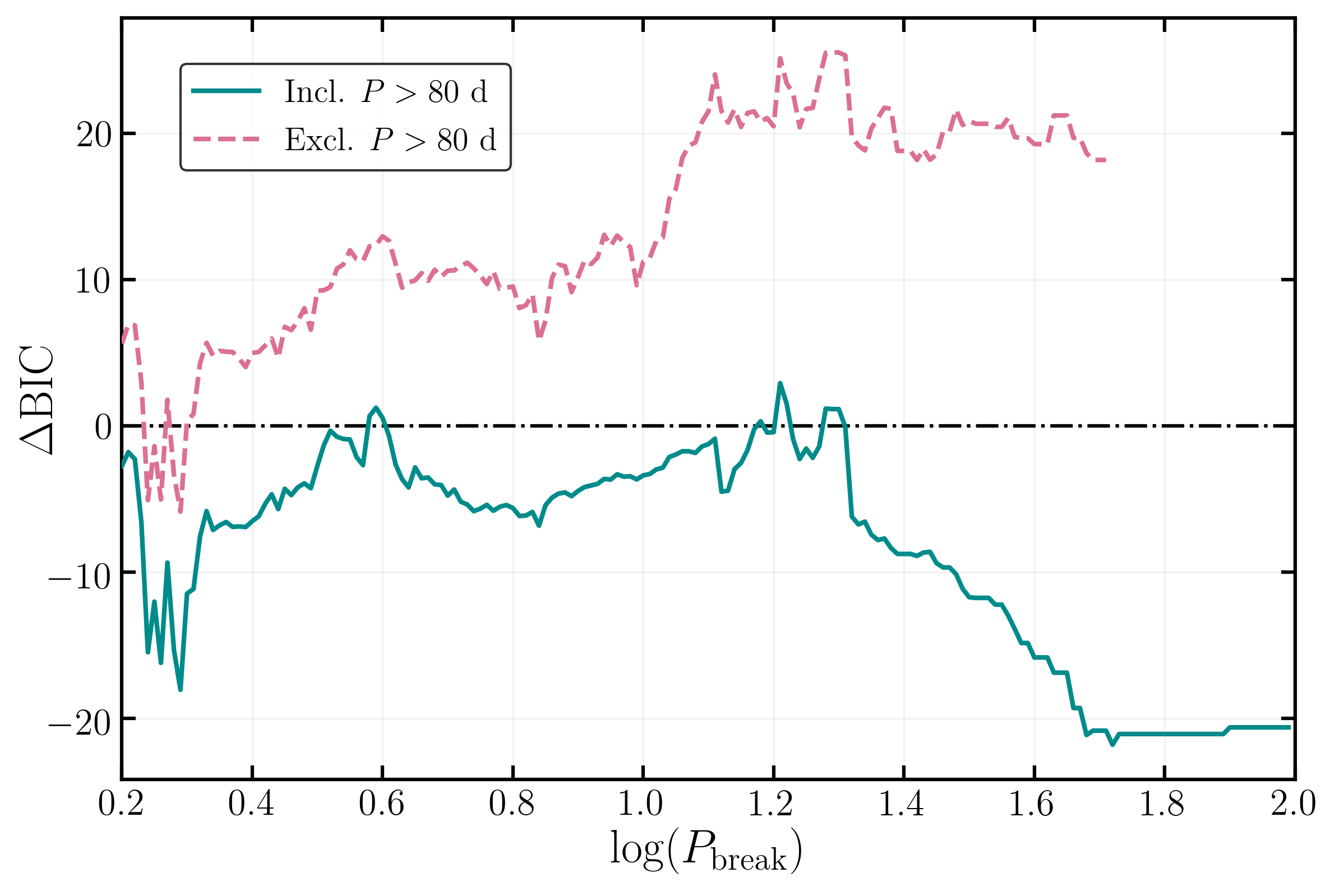
We compute the values for period breaks in steps. These results are shown in Figure 15 for the LMC Cepheids in the band. As with previous analysis, we have performed each fit twice to include (blue solid line) and exclude (pink dashed line) the ULP Cepheids. We find very different results depending on whether or not the four ULP Cepheids are included. Excluding these Cepheids, we find the vast majority of break values do not result in a significantly improved fit compared to a linear LL as . However, looking at the results for the ULP-included sample, we observe just how much the four ULP Cepheids influence the LL. Apart from three small spikes at and 1.3, the ULP-included results are negative across the entire period range, suggesting a non-linear relation is optimal. The minimum occurs at with , with values falling around this value for . values of this magnitude provide extremely strong evidence for a break at these long periods. For a break at , corresponding to 52.48 days, there are only 6 Cepheids in the long-period LL and 2305 in the short period LL. From this analysis, we conclude that there is sufficient evidence that suggests the ULP Cepheids do not follow the main LL and should be excluded from our final determination of the LL.
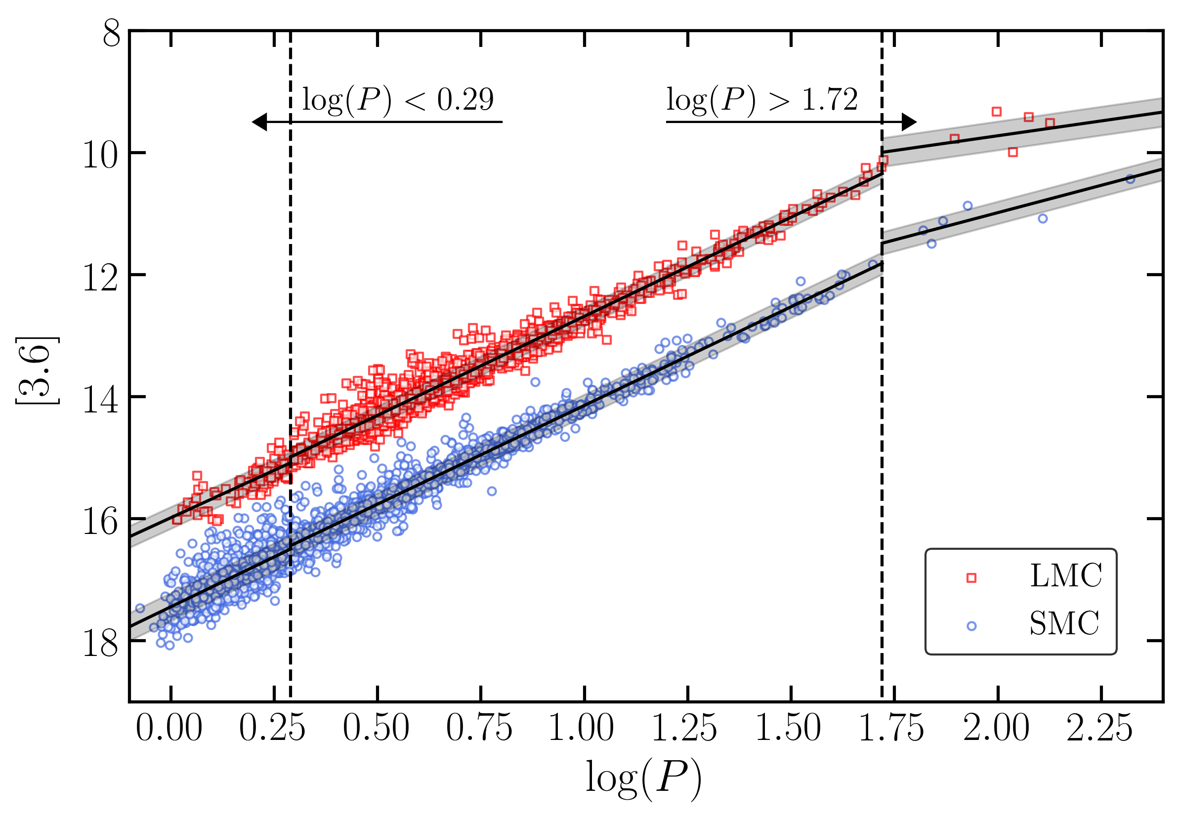
Aside from the large negative values that arise for when the ULP Cepheids are included, we also observe a large decline in for , with a minimum occurring at . This is the case regardless of whether the ULP Cepheids are included or not. Figure 16 shows the LMC and SMC Cepheid LLs based on period breaks at and , defining a short period LMC LL for given by
| (11) |
a main LMC LL for given by
| (12) |
and a long period LMC LL for given by
| (13) |
We now compare the use of these three LMC LLs, as shown in Figure 16, to the single linear relation shown in Figure 12. We find that the short period Cepheids with are more evenly distributed around their LL in Figure 16 compared to Figure 12, where we observe a larger proportion of Cepheids falling below the relation. At the long-period end of the relation, Figure 16 provides evidence that Cepheids with should be excluded from the main LL fit as they appear to follow a separate, much shallower relation entirely. Despite being penalised for using triple the number of parameters used by the standard linear relation, the three relations shown in Figure 16 and given by Equations 11 - 13 have , which is much more negative than the values for any of the relations with a single break point or no break point at all. Thus, we conclude that while we do not find strong evidence for a break midway through the LL, we do find that applying a small clipping at either end of the relation results in the optimal fit.
Figure 16 also shows the resulting SMC LLs when imposing breaks at and . We find that the SMC slopes are consistent with the equivalent LMC values over the same period range. However, the consistency in the and relations is only due to their slopes carrying large uncertainties. On the other hand, the main LLs for are consistent while also possessing small uncertainties. Over this period range, the LMC slope is and the SMC slope is . This suggests that the LL slopes are not affected by metallicity across this period range.
Lastly, we tested whether adding a quadratic term, such that
| (14) |
where are the coefficients of the quadratic, fits the data better. We found that , suggesting that a quadratic model can be confidently ruled out, and that a simple linear model is much more appropriate to describe the data.
6.2 Comparison of the Leavitt Law to the literature
| Galaxy | ||||||
|---|---|---|---|---|---|---|
| LMC | 0.155 | 2221 | ||||
| 0.151 | 2221 | |||||
| SMC | 0.180 | 1331 | ||||
| 0.177 | 1331 |
| Cepheid | b | b | |
|---|---|---|---|
| Cepc | 3.364 0.049 | ||
| CV Mon | |||
| S Nor | |||
| U Sgr | |||
| V367 Sct | |||
| V Cen | |||
| DL Cas | |||
| V340 Nor | |||
| CF Cas | |||
| TW Nor | |||
| Car | |||
| Gem | |||
| Dor | |||
| W Sgr | |||
| X Sgr | |||
| Y Sgr | |||
| FF Aql | |||
| T Vul | |||
| RT Aur |
-
Notes:
-
a Parallaxes in the top section are from the parallax of the Cepheid’s companion star or its host open cluster (Cantat-Gaudin et al. 2018; Breuval et al. 2020). These Cepheids were observed with Gaia and the values stated here have not had a zero-point offset applied. The parallaxes in the bottom section are from the HST Fine Guidance Sensors (Benedict et al., 2007). All values are given in milliarcseconds.
-
b and magnitudes are from M12.
-
c Cep was observed by both HST and Gaia. We decided to use the parallax value given by its companion star as it carried a smaller uncertainty.
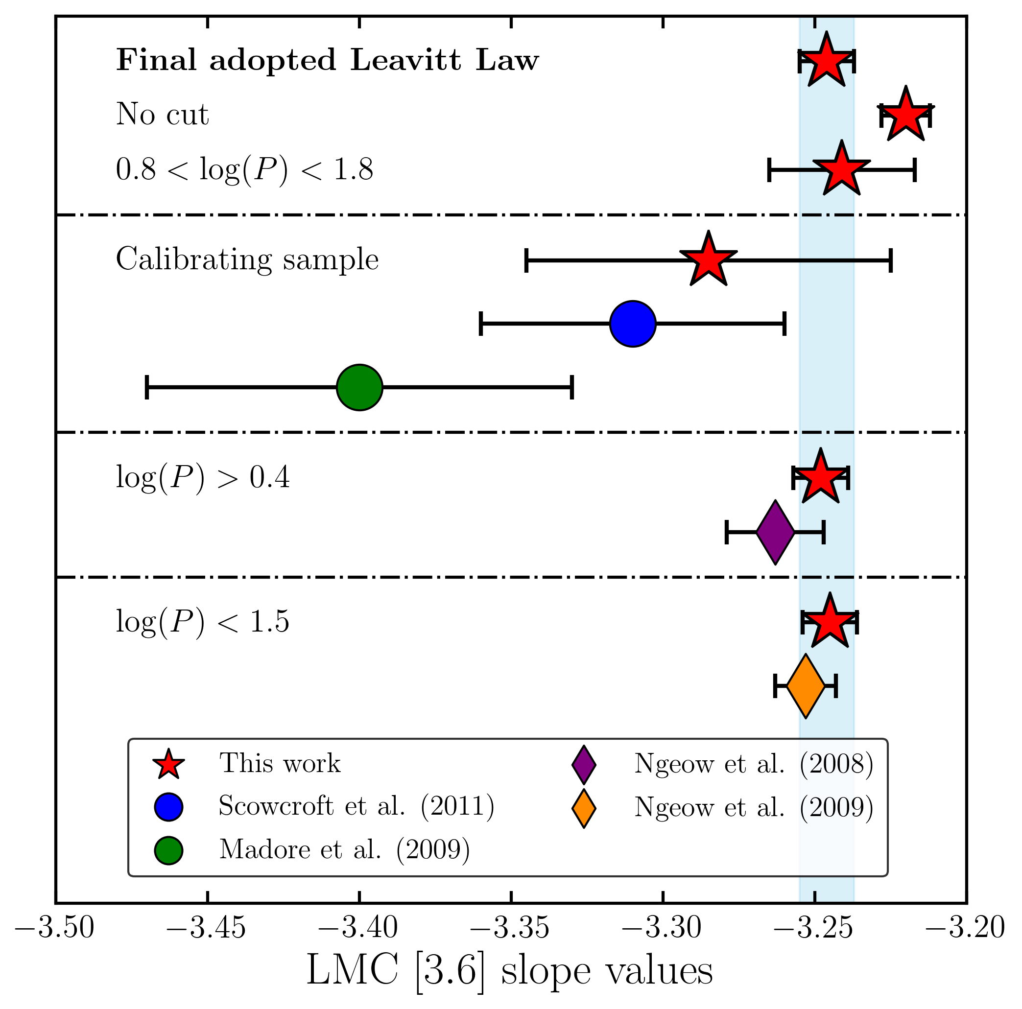
Observing campaigns have been performed that both serendipitously (e.g. SAGE) and purposefully (e.g. CHP) obtained mid-infrared observations of Cepheids in the Magellanic Clouds. We now compare our LL coefficients to those published in the literature. Our various relations with different period cuts are provided in Table 8. The slope values of the LMC LL are also shown in Figure 17.
Using the single-epoch measurements available at the time in the SAGE catalogue, Ngeow & Kanbur (2008) obtained the mid-IR LL in the LMC for all four Spitzer bands. The authors enforced a period cut of to remove possible contamination by overtone Cepheids. They then used iterative -clipping to obtain their LL coefficients. Comparing our LL for the LMC with no period cut applied, we find that our slope disagrees by just over . However, if we apply the same period cut and also only retain the one Cepheid with days that is common within both works, we obtain coefficients of and , which are now both consistent with the values from Ngeow & Kanbur (2008), within the stated uncertainties. Regardless of whether we apply a period cut or not, our LL is inconsistent with these works by at least . These discrepancies could be caused by a number of factors, including our sample being over three times larger, the use of template fitting rather than using single-epoch measurements, or the different pipelines used to obtain the photometry. In particular, the use of single-epoch measurements in the band are not appropriate due to the CO effect (Scowcroft et al., 2016a).
Building on their initial work, Ngeow et al. (2009) included an additional epoch of data and determined Cepheid mean magnitudes by averaging the two epochs to obtain the mid-IR LL using SAGE data. By cross-matching this data with the OGLE-III catalogue rather than OGLE-II, they were able to obtain the LL for a much larger sample size than their previous work. This time, the longest period Cepheids with were discarded. Similarly to the LL based off of single-epoch measurements, we find a consistent slope value when also employing the same period cut (), but inconsistent values in the band.
Both Madore et al. (2009b) and S11 use the sample of LMC Cepheids given in Persson et al. (2004) to obtain the mid-IR LL for 70 and 82 Cepheids, respectively. This is the same sample as our calibrating sample, with fully-phased observations and periods between 6 and 60 days. We see that these smaller samples give rise to steeper slopes than when many more Cepheids across the full period range are included. If we also restrict our sample to only include these longer period Cepheids, we obtain slopes of and for the and , respectively, which are consistent with S11 but not Madore et al. (2009b). However, if we further reduce our sample to only include the calibrating Cepheids, which are the identical set of Cepheids used by S11, we obtain slope values of and for the and , respectively. These values are very similar to those of S11, possibly suggesting that discrepancies in the LL are caused by the Cepheid sample selection, with bright, isolated, long period Cepheids being preferential targets. As Figure 1 shows, the majority of Cepheids in the Magellanic Clouds have short periods. Therefore, such criteria may not necessarily represent the entire Cepheid population.
Before our work, the only available SMC mid-IR relations that do not fix the slope of the relation to be that of the LMC are given by Ngeow & Kanbur (2010). Using only the first epoch of archival data taken as part of the SAGE-SMC program and applying iterative -clipping, they obtained the SMC LL coefficients for all Spitzer bands. Motivated by a potential slope change as different period cuts are employed (see their figure 4), they impose a break at and obtain the coefficients for both the short-period and long-period relations. We find consistent slope values for all relations except the short-period band, where it differs from the equivalent Ngeow & Kanbur (2010) relation by .
Overall, we find that our LL coefficients are in generally good agreement with those found in the literature, particularly when we apply the same period cuts to our sample.
6.3 Final calibrated Leavitt Law from Magellanic Cloud Cepheids
6.3.1 Final adopted Leavitt Law
For our final adopted LLs, we decided to only include Cepheids with periods , using 2221 LMC and 1331 SMC Cepheids in the fit. We excluded the Cepheids with , which includes the ULP Cepheids, as Section 6.1.3 showed that these Cepheids deviate from the fitted LL significantly and cause the LL to appear non-linear when they are included in the sample. Moreover, in Section 6.1.2, these ULP Cepheis were shown to affect the LL coefficients substantially. Therefore, it is best to remove these Cepheids, particularly as there is growing evidence that they follow their own independent LL (Bird et al. 2009; Fiorentino et al. 2012). We also excluded Cepheids with , as Section 6.1.3 provided strong evidence for a break in the LL at , with the shorter period Cepheids obeying a slightly shallower LL. As we showed in Section 6.1.2 that the LL coefficients are consistent up to , a period cut at does not affect the LL coefficients significantly.
Our adopted relations are given in Table 9. For the SMC relations, we fixed the slope to be that of the LMC and computed the SMC zero point. We chose to do this because the LMC slope is defined for a larger number of Cepheids and to also prevent biases that would be present due to the geometry of the SMC. This method of adopting the LMC slopes as fiducial is appropriate as the LMC and SMC slopes are consistent within and the slopes within for Cepheids with . The larger discrepancy in slopes is likely due to the effect of CO absorption on the magnitudes, while the magnitudes remain unaffected (Scowcroft et al., 2016a).
6.3.2 Zero point calibration
To calibrate the zero point, we combined the 10 MW Cepheids with geometric parallaxes determined by the Fine Guidance Sensors on-board the Hubble Space Telescope, as given in Benedict et al. (2007), with 10 MW Cepheids that have Gaia DR2 parallaxes determined by either their companion star or their host open cluster (Cantat-Gaudin et al. 2018; Breuval et al. 2020). For the Gaia parallaxes, we applied a parallax zero-point offset value of -46 13 as, as determined by Riess et al. (2018). The size of the parallax zero-point offset may depend on the object’s colour and magnitude (Lindegren et al., 2018). Therefore, we use the value from Riess et al. (2018) as it was derived from MW Cepheids. Our sample of MW stars were chosen as they all have mid-IR mean magnitudes from M12. The parallaxes and magnitudes for these Cepheids are provided in Table 10. For Cep, both HST and Gaia parallaxes were available. We decided to use the Gaia parallax, as it carried a smaller uncertainty.
The calibrated zero point was computed using the Astrometric Based Luminosity (ABL) (Feast & Catchpole 1997; Arenou & Luri 1999), defined as
| (15) |
where is fixed from the apparent magnitude LL, is the parallax in milliarcseconds and is the dereddened apparent magnitude. We fit the relation using curve_fit from the scipy library in Python to determine the value of the zero point, . We find calibrated zero points of and for the and band, respectively.
Using the calibrated LL and the zero points for each galaxy, we calculated the apparent distance modulus of the LMC to be mag and the SMC to be mag. The differential distance modulus is mag. This result is in agreement with several other differential distance measurements from Cepheids including Groenewegen (2000) ( mag), Bono et al. (2010) ( mag), Inno et al. (2013) ( mag) and S16 ( mag). Our result is also consistent with differential distance measurements from other methods such as eclipsing binaries (Graczyk et al., 2014, mag) and RR Lyrae stars (Szewczyk et al., 2009, mag).
7 Summary
Using mid-IR observations of fundamental mode Classical Cepheids in the Magellanic System, we have constructed the and LL for the Magellanic Clouds. Through our MCMC template light curve fitting procedure, where the templates were constructed from a subsample of Cepheids with well-sampled light curves from the CHP, we have obtained mid-IR mean magnitudes for all Cepheids within the SAGE footprint, amounting to 2311 LMC and 2637 SMC Cepheids. Our catalogue containing and mean magnitudes for these Cepheids is given in Table 7, with the entire catalogue available for online download. This catalogue will be used in a companion paper (Chown et al. 2020, in prep) to study the 3D structure of the Magellanic System.
The LMC LL is the primary relation used in distance determination. We investigated the dependence of the coefficients of this LL on various period cuts. When excluding the ultra-long period Cepheids (ULP) (those with periods > 80 days), we find that our relation is unaffected by period cuts below , as the slope and zero point remain consistent with the relation that uses the entire sample.
In addition, we investigated the non-linearity of the LMC LL. We used the Bayesian Information Criterion (BIC) to quantify our results. Our results varied greatly depending on whether the ULP Cepheids were included, with strong evidence for a linear relation when excluding them and strong evidence for a non-linear relation when including them. We found that the most likely periods for a break to occur were at and .
Our final adopted relations make use of these results and only include Cepheids with , resulting in 2221 LMC and 1331 SMC Cepheids being used in the LL fit. We showed in Section 6.1.2 that a period cut at does not affect the slope and zero point significantly. The break value at was used to exclude the ULP Cepheids, as these Cepheids were shown in Section 6.1.3 to follow a much shallower LL. Using parallaxes of Cepheids in the Milky Way from both the Hubble Space Telescope and Gaia, we calibrated the zero point of our LL using the Astrometric Based Luminosity. Our final relations are given by
| (16) | ||||
| (17) |
Acknowledgements
We thank the anonymous referee for their valuable comments which have significantly improved our paper. The authors would like to thank Raoul and Catherine Hughes for awarding the RCH Alan Hunter Scholarship to fund this research. This work is based on observations made with the Spitzer Space Telescope, which is operated by the Jet Propulsion Laboratory, California Institute of Technology under a contract with NASA. This work makes use of the Optical Gravitational Lensing Experiment (OGLE) Collection of Variable Stars database. This research made use of Astropy,888http://www.astropy.org a community-developed core Python package for Astronomy (Astropy Collaboration et al., 2013; Price-Whelan et al., 2018).
Data availability
The data underlying this article are from Chown et al. (2020). The code used for this article are available at https://github.com/abichown/DAOPHOT-Scripts.
References
- Arenou & Luri (1999) Arenou F., Luri X., 1999, in Egret D., Heck A., eds, Astronomical Society of the Pacific Conference Series Vol. 167, Harmonizing Cosmic Distance Scales in a Post-HIPPARCOS Era. pp 13–32 (arXiv:astro-ph/9812094)
- Astropy Collaboration et al. (2013) Astropy Collaboration et al., 2013, A&A, 558, A33
- Benedict et al. (2007) Benedict G. F., et al., 2007, The Astronomical Journal, 133, 1810
- Bird et al. (2009) Bird J. C., Stanek K. Z., Prieto J. L., 2009, ApJ, 695, 874
- Bono et al. (2010) Bono G., Caputo F., Marconi M., Musella I., 2010, Astrophysical Journal, 715, 277
- Breuval et al. (2020) Breuval L., et al., 2020, arXiv e-prints, p. arXiv:2006.08763
- Cantat-Gaudin et al. (2018) Cantat-Gaudin T., et al., 2018, A&A, 618, A93
- Cardelli et al. (1989) Cardelli J. A., Clayton G. C., Mathis J. S., 1989, Astrophysical Journal, 345, 245
- Chown et al. (2020) Chown A., Scowcroft V., Wuyts S., 2020, “The mid-infrared Leavitt Law for Classical Cepheids in the Magellanic Clouds” by Chown et al. (2020). Bath: University of Bath Research Data Archive, https://doi.org/10.15125/BATH-00915
- Cioni et al. (2011) Cioni M. R. L., et al., 2011, A&A, 527, A116
- Fabozzi et al. (2014) Fabozzi F. J., Focardi S. M., Rachev S. T., Arshanapalli B. G., 2014, The Basics of Financial Econometrics: Tools, Concepts, and Asset Management Applications. John Wiley & Sons, Inc., Hoboken, New Jersey
- Fazio et al. (2004) Fazio G. G., et al., 2004, The Astrophysical Journal Supplement Series, 154, 10
- Feast & Catchpole (1997) Feast M. W., Catchpole R. M., 1997, MNRAS, 286, L1
- Fiorentino et al. (2012) Fiorentino G., et al., 2012, Ap&SS, 341, 143
- Foreman-Mackey et al. (2013) Foreman-Mackey D., Hogg D. W., Lang D., Goodman J., 2013, PASP, 125, 306
- Fouqué et al. (2007) Fouqué P., et al., 2007, Astronomy & Astrophysics, 476, 73
- Freedman et al. (2011) Freedman W. L., et al., 2011, Astronomical Journal, 142, 192
- Gieren et al. (2005) Gieren W., Storm J., Barnes Thomas G. I., Fouqué P., Pietrzyński G., Kienzle F., 2005, ApJ, 627, 224
- Gordon et al. (2011) Gordon K. D., et al., 2011, AJ, 142, 102
- Graczyk et al. (2014) Graczyk D., et al., 2014, ApJ, 780, 59
- Groenewegen (2000) Groenewegen M. A. T., 2000, A&A, 363, 901
- Groenewegen (2018) Groenewegen M. A. T., 2018, A&A, 619, A8
- Hertzsprung (1926) Hertzsprung E., 1926, Bull. Astron. Inst. Netherlands, 3, 115
- Indebetouw et al. (2005) Indebetouw R., et al., 2005, Astrophysical Journal, 619, 913
- Inno et al. (2013) Inno L., et al., 2013, Astrophysical Journal, 764, 84
- Inno et al. (2015) Inno L., et al., 2015, A&A, 576, A30
- Joshi & Panchal (2019) Joshi Y. C., Panchal A., 2019, A&A, 628, A51
- Kodric et al. (2015) Kodric M., et al., 2015, ApJ, 799, 144
- Leavitt (1908) Leavitt H. S., 1908, Annals of Harvard College Observatory, 60, 87
- Leavitt & Pickering (1912) Leavitt H., Pickering C., 1912, Harvard College Observatory, 173, 1
- Lindegren et al. (2018) Lindegren L., et al., 2018, A&A, 616, A2
- Macri et al. (2015) Macri L. M., Ngeow C.-C., Kanbur S. M., Mahzooni S., Smitka M. T., 2015, AJ, 149, 117
- Madore et al. (2009a) Madore B. F., Rigby J., Freedman W. L., Persson S. E., Sturch L., Mager V., 2009a, ApJ, 693, 936
- Madore et al. (2009b) Madore B. F., Freedman W. L., Rigby J., Persson S. E., Sturch L., Mager V., 2009b, The Astrophysical Journal, 695, 988
- Makovoz & Khan (2005) Makovoz D., Khan I., 2005, in Shopbell P., Britton M., Ebert R., eds, Astronomical Society of the Pacific Conference Series Vol. 347, Astronomical Data Analysis Software and Systems XIV. p. 81
- Meixner et al. (2006) Meixner M., et al., 2006, The Astronomical Journal, 132, 2268
- Mighell et al. (2008) Mighell K. J., Glaccum W., Hoffmann W., 2008, in Space Telescopes and Instrumentation 2008: Optical, Infrared, and Millimeter. p. 70102W, doi:10.1117/12.789801
- Moffett et al. (1998) Moffett T. J., Gieren W. P., Barnes Thomas G. I., Gómez M., 1998, ApJS, 117, 135
- Monson et al. (2012) Monson A. J., Freedman W. L., Madore B. F., Persson S. E., Scowcroft V., Seibert M., Rigby J. R., 2012, Astrophysical Journal, 759, 146
- Ngeow & Kanbur (2008) Ngeow C., Kanbur S. M., 2008, ApJ, 679, 76
- Ngeow & Kanbur (2010) Ngeow C. C., Kanbur S. M., 2010, Astrophysical Journal, 720, 626
- Ngeow et al. (2005) Ngeow C.-c., Kanbur S. M., Nikolaev S., Buonaccorsi J., Cook K. H., Welch D. L., 2005, Monthly Notices of the Royal Astronomical Society, 363, 831
- Ngeow et al. (2008) Ngeow C., Kanbur S. M., Nanthakumar A., 2008, A&A, 477, 621
- Ngeow et al. (2009) Ngeow C.-C., Kanbur S. M., Neilson H. R., Nanthakumar A., Buonaccorsi J., 2009, ApJ, 693, 691
- Ngeow et al. (2015) Ngeow C.-C., Kanbur S. M., Bhardwaj A., Singh H. P., 2015, ApJ, 808, 67
- Persson et al. (2004) Persson S. E., Madore B. F., Krzemin W., Freedman W. L., Roth M., Murphy D. C., 2004, The Astronomical Journal, 128, 2239
- Price-Whelan et al. (2018) Price-Whelan A. M., et al., 2018, AJ, 156, 123
- Reach et al. (2005) Reach W. T., et al., 2005, Publications of the Astronomical Society of the Pacific, 117, 978
- Riebel et al. (2015) Riebel D., et al., 2015, Astrophysical Journal, 807, 1
- Riess (2019) Riess A. G., 2019, Nature Reviews Physics, 2, 10
- Riess et al. (2018) Riess A. G., et al., 2018, ApJ, 861, 126
- Ripepi et al. (2016) Ripepi V., et al., 2016, The Astrophysical Journal Supplement Series, 224, 21
- Sandage et al. (2009) Sandage A., Tammann G. A., Reindl B., 2009, A&A, 493, 471
- Schwarz (1978) Schwarz G., 1978, Annals of Statistics, 6, 461
- Scowcroft et al. (2009) Scowcroft V., Bersier D., Mould J. R., Wood P. R., 2009, MNRAS, 396, 1287
- Scowcroft et al. (2011) Scowcroft V., Freedman W., Madore B. F., Monson A. J., Persson S. E., Seibert M., Rigby J. R., Sturch L., 2011, Astrophysical Journal, 743, 76
- Scowcroft et al. (2016a) Scowcroft V., Seibert M., Freedman W. L., Beaton R. L., Madore B. F., Monson A. J., Rich J. A., Rigby J. R., 2016a, MNRAS, 459, 1170
- Scowcroft et al. (2016b) Scowcroft V., Freedman W. L., Madore B. F., Monson A., Persson S. E., Rich J., Seibert M., Rigby J. R., 2016b, ApJ, 816, 49
- Soszynski et al. (2005) Soszynski I., Gieren W., Pietrzynski G., 2005, Publications of the Astronomical Society of the Pacific, 117, 823
- Soszyński et al. (2015) Soszyński I., et al., 2015, Acta Astronomica, 65, 297
- Soszyński et al. (2017) Soszyński I., et al., 2017, Acta Astron., 67, 103
- Stetson (1987) Stetson P. B., 1987, Publications of the Astronomical Society of the Pacific, 99, 191
- Stetson (1994) Stetson P. B., 1994, Publications of the Astronomical Society of the Pacific, 106, 250
- Stetson & Harris (1988) Stetson P. B., Harris W. E., 1988, Astronomical Journal, 96, 3
- Szewczyk et al. (2009) Szewczyk O., Pietrzyński G., Gieren W., Ciechanowska A., Bresolin F., Kudritzki R.-P., 2009, AJ, 138, 1661
- Tammann et al. (2003) Tammann G. A., Sandage A., Reindl B., 2003, Astronomy & Astrophysics, 448, 423
- Udalski et al. (1999) Udalski A., Szymański M. K., Kubiak M., Pietrzyński G., Soszyński I., Wozniak P., Zebrun K., 1999, Acta Astronomica, 49, 201
- Udalski et al. (2008) Udalski A., Szymanski M. K., Soszynski I., Poleski R., 2008, Acta Astron., 58, 69
Appendix A Mid-infrared light curves for the calibrating Cepheids
We present the full sample of calibrating sample Cepheids in Figure 18 of the online version.
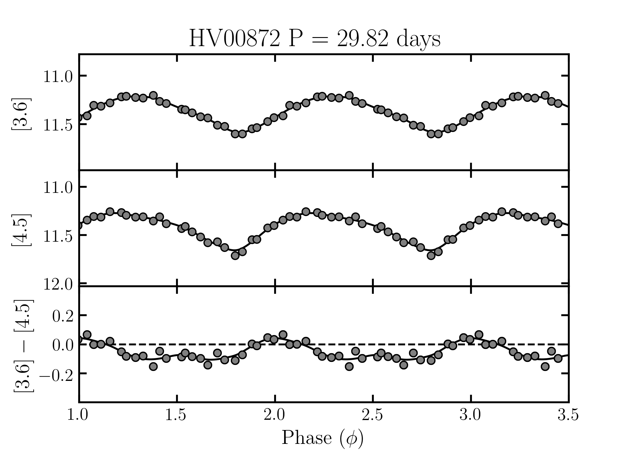
Appendix B Choice of priors
In Section 4.3, we discussed several uniform priors that were used in our MCMC template fitting method. These priors were imposed on the and mean magnitudes, amplitudes and phases and were based on Figure 19. A uniform prior was placed on the mid-IR amplitude ratios (top panel of Figure 19), the mid-IR magnitude ratio (middle panel of Figure 19), and mid-IR phase lag (bottom panel of Figure 19). In each of the panels, the distribution appears Gaussian. However, we opted for a uniform prior as we found that when using a Gaussian prior resulted in the MCMC walkers being unable to explore the parameter space fully.
In the middle panel of Figure 19, there appears to be a negative correlation for , with an inversion for . This shape mimics the period-colour relation shown in Scowcroft et al. (2016a) (their figure 5).