Wolf–Rayet stars in the Antennae unveiled by MUSE

Abstract

We present the analysis of archival Very Large Telescope (VLT) Multi Unit Spectroscopic Explorer (MUSE) observations of the interacting galaxies NGC 4038/39 (a.k.a. the Antennae) at a distance of 18.1 Mpc. Up to 38 young star-forming complexes with evident contribution from Wolf–Rayet (WR) stars are unveiled. We use publicly available templates of Galactic WR stars in conjunction with available photometric extinction measurements to quantify and classify the WR population in each star-forming region, on the basis of its nearly Solar oxygen abundance. The total estimated number of WR stars in the Antennae is 4053 $\pm$ 84, of which there are 2021 $\pm$ 60 WNL and 2032 $\pm$ 59 WC-types. Our analysis suggests a global WC to WN-type ratio of 1.01 $\pm$ 0.04, which is consistent with the predictions of the single star evolutionary scenario in the most recent BPASS stellar population synthesis models.

1 INTRODUCTION

Most star formation occurs in groups and associations that were once embedded in Giant Molecular Clouds (Lada & Lada, 2003). Observational evidence shows that star formation is enhanced in interacting and merging galaxies (see, e.g., Smith et al., 2007; Li et al., 2008; Knapen et al., 2015), making them ideal environments to study the formation and evolution of stars and, in particular young massive stars (Whitmore, 2009). Super star clusters (SSCs), objects as compact and massive as globular clusters (GC), though younger, are particularly abundant in starburst and interacting galaxies. The most massive and compact of these are the ones expected to survive the disruptive effects of gravitational shocks for a Hubble time, and hence are thought to be the progenitors of GC (Portegies-Zwart et al., 2010).

Wolf–Rayet (WR) stars are considered descendants of O-type stars ($M_{\mathrm{ZAMS}}\gtrsim 25$ M_⊙; Crowther, 2007, and references therein). For this reason, they are often used as indicators of young stellar populations ($\sim$2–4 Myr) and to study the chemical enrichment of its environments due to their characteristic strong stellar winds enhanced with processed elements (see, e.g., Maeder, 1992). They are also considered to be the most suitable candidates for core collapse supernovae (SN) Ibc and long-duration soft-gamma ray burst (Woosley & Heger, 2006; Woosley & Bloom, 2006). There is a clear need to increase the sample of WR stars in the local Universe, as that would raise the probability of a previously classified WR exploding as a SN in a reasonable human life-time (Moffat, 2015). Up to now, not a single known WR star has exploded.

NGC 4038/39, better known as the Antennae galaxies, are located at a distance of 18.1 Mpc ($m-M=31.29$; Riess et al., 2016), making them the nearest and youngest pair of colliding galaxies at an early stage of a merger (Whitmore & Schweizer, 1994). Due to the significant number of star forming zones and giant H ii regions in the Antennae, many multi-wavelength imaging (e.g., Zhang et al., 2001; Metz et al., 2004; Matthews et al., 2018) and spectroscopic studies (e.g., Whitmore et al., 2005; Weilbacher et al., 2018; Gunawardhana et al., 2019) have been conducted so far.

Optical studies of the Antennae have revealed the presence of WR stars in the past. Bastian et al. (2006) presented Very Large Telescope (VLT) VIMOS integral-field spectroscopy of two northern fields in the Antennae and reported five SSCs with strong WR features. Later, Bastian et al. (2009) presented Gemini GMOS observations and reported the discovery of seven additional SSCs with broad WR signatures. Nevertheless, a dedicated search for WR stars, specifying their number, classification and distribution has not been performed yet.

Extragalactic spectroscopic observations, such as those obtained with the Multi Unit Spectroscopic Explorer (MUSE) at the VLT, are powerful tools that can be used to unveil the presence of WR stars in the nearby Universe. It is important to note that at large distances most findings of WR features correspond to unresolved populations of stars in stellar clusters, rather than single stars.

In this paper we present the analysis of archival VLT MUSE observations of the prototypical starburst/merging galaxy, the Antennae. The MUSE data cubes were searched to identify tens of SSC complexes with WR features, significantly increasing the sample of relatively nearby extragalactic WR stars and SN candidates. Publicly available templates of Galactic WR stars were used to quantify and classify the WR population in each region. We compare our observed results with the predictions of stellar population synthesis models.

This paper is organised as follows. In Section 2, we describe the observations, technical details of the data preparation and the search for WR features. In Section 3, we present our classification and quantification scheme resulting from the spectral analysis. The discussion of our results is presented in Section 4, and the conclusions are listed in Section 5.

2 OBSERVATIONS

2.1 Public VLT MUSE data cubes

MUSE is a panoramic integral-field spectrograph at the 8 m VLT of the European Southern Observatory (ESO), operating in the optical wavelength range from 4600 to 9300 Å  with a spatial sampling of 0.2 arcsec pixel^-1, a spectral sampling of 1.25 Å pixel^-1 and a spectral resolution $\sim$3 Å (Bacon et al., 2010).

Public MUSE data cubes covering the entire Antennae galaxies were retrieved from the ESO Science Archive Facility. The data cubes were already flux and wavelength calibrated, ready for scientific exploitation. The data were obtained during three observing runs on 2015 April 22–24, 2015 May 11–23 and 2016 February 01 (PI: P. M. Weilbacher). The observations correspond to a total of 23 data sets, several of them covering the same regions in NGC 4038/39, which amounts to a total exposure time of $\approx$22.9 h. Details of the observations have been presented in Weilbacher et al. (2018) and Gunawardhana et al. (2019). A schematic view of all the field of views (FoV) of all the observations is shown in Fig. 18 left panel in Appendix A.

2.2 Search and distribution of WR features

WR stars are spectroscopically identified by the presence of two broad features, the blue bump (BB) at $\sim$4686 Å  and the red bump (RB) at $\sim$5808 Å. These features are the result of blends of several ionic transitions. The BB contains one or several of the He ii, N iii, N v, C iii and C iv lines, whereas the RB is made of C iv lines. WR stars exhibiting any nitrogen line are classified as WN-type, whereas those containing a carbon line are of WC-type (see details in Section 3).

We inspected the MUSE data cubes searching for spectral WR features and detected their presence in four of these fields. The outskirts of the Antennae did not show any hint of WR emission. Consequently, in the present paper we only use the four observations that cover the main regions in the Antennae (see Fig. 18 right panel). Details of these data cubes are listed in Table 4 in Appendix A.

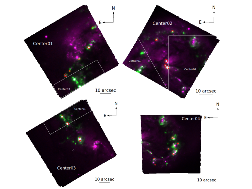
Figure 19: Colour-composite images created from the four MUSE datasets, simulating narrow-band filters, each with 3 Å of bandwidth, centered on 4680 Å (redshifted wavelength of He ii- blue), 4800 Å (continuum -red) and 6596 Å (redshifted wavelength of H$\alpha$- green). The position of WR features were identified by inspecting the images are shown with red circle. Subsequent search in IFU spectra revealed the presence of other WR features, which we identify with green circles.

To identify WR stars in the Antennae, we used the data cubes to create three different images simulating narrow-band filters, each with 3 Å of bandwidth, centered on 4680 Å (BB), 4800 Å (continuum) and 6596 Å (H$\alpha$), taking into account the redshift of Antennae ($z\sim$0.005). Then we used colour-composite images in order to highlight any WR emission at 4686 Å to facilitate its detection. The resultant colour-composite images of the four FoV presenting WR features are shown in Fig. 19 in Appendix A.

We used the QFitsView datacube file viewer (Ott, 2012) to extract spectra from all the identified candidates to confirm them as bona fide WR detections. Subsequently, we followed a meticulous inspection by-eye of images and spectra, simultaneously, in order to rule out probable WR presence in places without an apparent excess in the BB band, and also to identify any faint BB that did not show up in the colour images. As a result, several weak-WR objects were included.

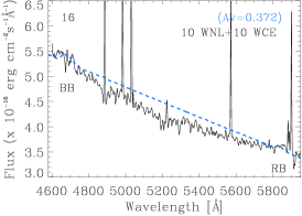
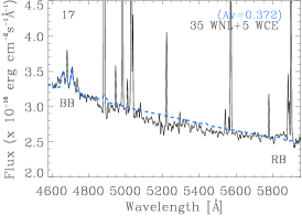
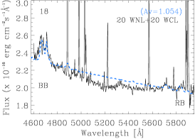
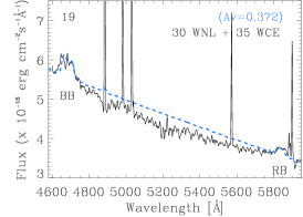
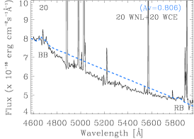
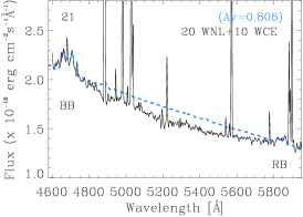
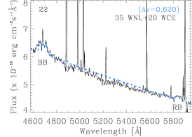
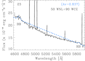
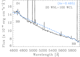
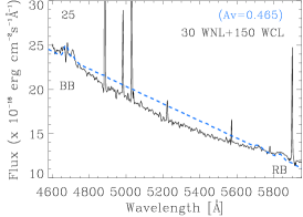
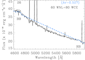
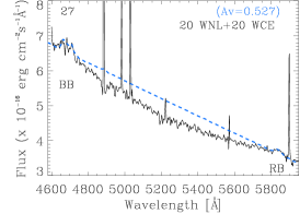
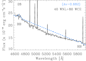
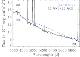
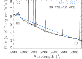
Figure 5: – continued

We note that not every emission feature detected in the BB is a WR finding. The spectrum of a spurious WR candidate, probably a quasar at $z\sim 0.264$, was found in one of the data cubes. Its spectrum is presented in Fig. 20 of Appendix B. These kinds of objects can mimic WR features when some of its broad emission lines, at a given redshift, coincide precisely with the wavelength of a WR feature. This is uncommon, but happens (see, e.g., figure 5 in Neugent et al., 2012), and care must be taken not to confuse the nature of these objects when using the narrow-band filter searching technique alone. The analysis of the spectral properties of this object are out of the scope of the present work.

In order to quantify and classify the presence of WR stars in the Antennae galaxies, we need spectra of each of the SSCs in which they are found. The main criterion to choose the size of the spectral extraction aperture was to maximise the intensity of the WR features. Small apertures would underestimate the WR bump intensities whilst apertures larger than necessary could dilute these line profiles.

We obtained a final sample of 38 spectra with confirmed WR features. Their distribution is shown in the colour-composite Hubble Space Telescope (HST) image presented in Fig. 1. Its locations are shown with red circles and labeled from 1 to 38. As an example, we present in Fig. 2 the MUSE spectrum of WR 1 which displays the prominent BB and RB features. Other narrow emission lines indicated correspond to the nebular environment of the object.

2.3 Public archival GTC OSIRIS spectra

As described above, the VLT MUSE spectra are suitable for looking the so-called BB and RB. However, given the spectral coverage of MUSE, we do not have access to another important WR feature, the violet bump (VB) at $\sim$3820 Å. This broad emission is indispensable to reveal (or discard) the presence of Oxygen-type WR stars (WO).

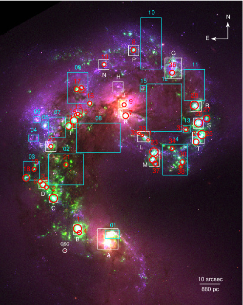
Figure 1: Colour-composite HST ACS image of the Antennae galaxies. Red, green and blue correspond to the F814W, F658W and F435W broad-band filters, respectively. The locations of the 38 star-forming complexes with WR features are shown with red circles. The white and cyan boxes correspond to the knots (letters: A–T) and regions (number IDs: 01–15), respectively, studied by Whitmore et al. (2010), who report the reddening information used in this study. The extinction values and the angular and physical aperture sizes are listed in Table 1. The position of a detected quasar is denoted with a circle labeled as qso.

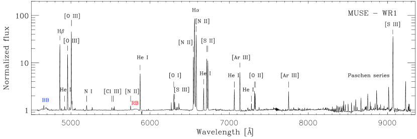
Figure 2: VLT MUSE redshift corrected spectrum of WR 1 in the Antennae. The blue bump (BB) at 4686 Å, and the red bump (RB) at 5808 Å, the most common optical WR features, are indicated, as well as the narrow lines from the nebular environment. The spectrum is shown normalized to the best fit continuum spectrum.

Figure 3: GTC OSIRIS spectrum of WR 1, complementary to that of MUSE. The WR features BB and RB as well as some important nebular lines are identified. The spectrum is shown normalized to the best fit continuum spectrum.

Looking to cover this wavelength range, we also retrieved available public archival observations in the Antennae from the OSIRIS spectrograph in long-slit mode (Cabrera-Lavers, 2016), at the 10.4 m Gran Telescopio de Canarias (GTC). The OSIRIS spectrum covers a spectral range from 3700 to 7500 Å  and is appropriate to take a look in the VB band. Unfortunately, only one of the identified WR features in the Antennae has been detected by the OSIRIS observation, WR 1.

These observations were carried out on 2013 January 12 in service mode (PI: C. M. Gutiérrez). The total observing time was 2700 s which was split into three blocks of 900 s, facilitating later removal of cosmic rays. The settings were: R1000B grism, slitwidth of 1 arcsec, position angle of $235.15^{\circ}$, spectral resolution of $\sim$7 Å  and a CCD binning of 2$\times$2. The observations have a spatial scale of 0.254 arcsec pixel^-1 and a spectral sampling of $\sim$2 Å pixel^-1. The ancillary files contained the spectrophotometric standard GD140 (2.5 arcsec slitwidth), $10\times$Bias (100 KHz), $8\times$Flats (1.23 arcsec slitwidth) and the arc lamps: $2\times$HgAr, $2\times$Ne (1 arcsec slitwidth). The night was clear of clouds, with Dark Moon, and a seeing of 1.03 arcsec. The reduction and extraction procedure we followed was similar to that described in detail by Gómez-González et al. (2016).

The resultant spectrum of WR 1 covers a complementary bluer wavelength range to that of MUSE and is shown in Fig. 3. With this valuable information, the presence of WO-type stars in this SSC can be discarded.

2.4 Extinction correction

In order to deredden our WR spectra, we used the results presented by Whitmore et al. (2010), who used HST ACS observations to produce $U-B$ versus $V-I$ colour-colour diagrams to study the extinction across the Antennae galaxies. These authors studied different star-forming knots and regions which we mark with white and cyan rectangles, respectively, in Fig. 1. It is worth mentioning that all of our WR detections lie within some of their analysed fields.

The $E(B-V)$ values were taken from Whitmore et al. (2010) and correspond to those listed in their table 9 (column 8). With this information we determined the visual extinction values ($A_{\mathrm{V}}$) for each WR listed in Table 1. We use a standard total-to-selective extinction of $R_{\mathrm{V}}=3.1$ and the equation $A_{\mathrm{V}}=3.1E(B-V)$.

The dereddened spectra of all the 38 WR sources in the Antennae galaxies obtained from the MUSE observations are presented in Fig. 4. These spectra were fitted with template WR spectra to infer the number and type of WR stars in each identified source following the method described below.

3 Classification and number of WR

3.1 Galactic templates

Template fitting has proven to be a very helpful tool to study extragalactic WR stars in unresolved massive stellar populations (e.g., Hadfield & Crowther, 2006; Kehrig et al., 2013; Gómez-González et al., 2016, 2020). The method consists in comparing the spectra with templates obtained from averaging observed spectra of a number of individual classified WR stars in the Galaxy and the Magellanic Clouds. This methodology has been thoroughly described in Gómez-González et al. (2020). However, here we give a brief description of the quantification and classification procedure of the 38 regions with WR features in the Antennae.

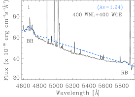
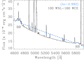
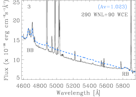
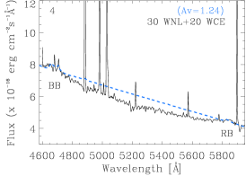
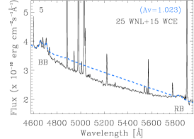
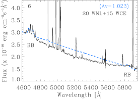
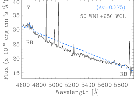
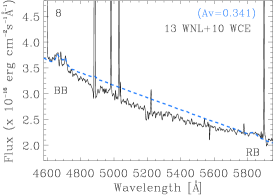
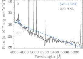
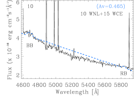
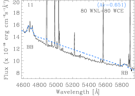
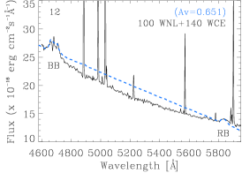
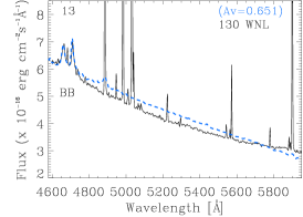
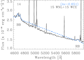
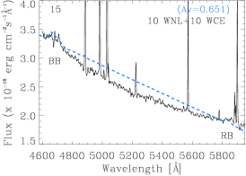
Figure 4: VLT MUSE spectra shown in the range of the BB and RB for the 38 star-forming complexes with WR features in the Antennae, corrected by the extinction values reported in Whitmore et al. (2010) (solid line), along with their best fit Galactic templates (blue dashed line). The identification number of the WR region, the name of the templates and their multiplicative factors required to match the observed bump strengths, as well of their $A_{\rm V}$ values, are indicated. The results are listed in Table 1.

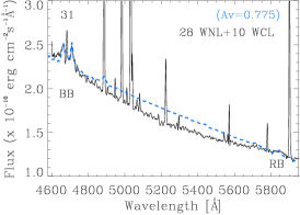
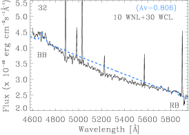
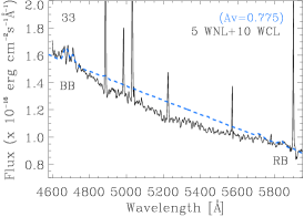
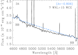
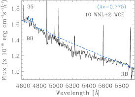
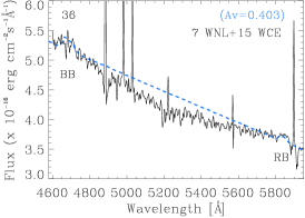
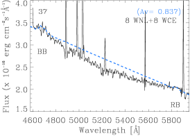
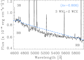
Figure 6: – continued

We use templates of individual Galactic WR stars, publicly available from the personal website of P. Crowther. Galactic templates are suitable for the Antennae on the basis of its nearly Solar metallicity (see Bastian et al., 2009), with a flat metallicity gradient (see Lardo et al., 2015). Furthermore, below we confirm that this is valid for our objects.

Table 1: WR stars in star-forming complexes of the Antennae galaxies^†.

ID	Classification & number				WC/WN	O	WR/O	Zone	$A_{\rm V}$	$D_{\rm aper}$
	WNL	WCE	WCL	WR					(mag)	(′′)	(pc)
(1)	(2)	(3)	(4)	(5)	(6)	(7)	(8)	(9)	(10)	(11)	(12)
1	400 $\pm$ 40	400 $\pm$ 40	$\cdots$	800 $\pm$ 57	1.00 $\pm$ 0.14	2196 $\pm$ 5	0.36 $\pm$ 0.03	B	1.2	4.0	351.0
2	100 $\pm$ 10	160 $\pm$ 16	$\cdots$	260 $\pm$ 19	1.60 $\pm$ 0.23	1566 $\pm$ 4	0.17 $\pm$ 0.01	C	1.0	4.0	351.0
3	290 $\pm$ 29	90 $\pm$ 9	$\cdots$	380 $\pm$ 30	0.31 $\pm$ 0.04	1153 $\pm$ 3	0.33 $\pm$ 0.03	D	1.0	2.8	245.7
4	30 $\pm$ 3	20 $\pm$ 2	$\cdots$	50 $\pm$ 4	0.67 $\pm$ 0.09	225 $\pm$ 2	0.22 $\pm$ 0.02	B	1.2	2.0	175.5
5	25 $\pm$ 3	15 $\pm$ 2	$\cdots$	40 $\pm$ 3	0.60 $\pm$ 0.11	333 $\pm$ 1	0.12 $\pm$ 0.01	D	1.0	2.0	175.5
6	20 $\pm$ 2	15 $\pm$ 2	$\cdots$	35 $\pm$ 3	0.75 $\pm$ 0.13	296 $\pm$ 1	0.12 $\pm$ 0.01	D	1.0	2.0	175.5
7	50 $\pm$ 5	$\cdots$	250 $\pm$ 25	300 $\pm$ 25	5.00 $\pm$ 0.54	981 $\pm$ 9	0.31 $\pm$ 0.03	K	0.8	2.8	245.7
8	13 $\pm$ 1	10 $\pm$ 1	$\cdots$	23 $\pm$ 2	0.77 $\pm$ 0.10	233 $\pm$ 2	0.10 $\pm$ 0.01	10	0.3	2.4	210.6
9	200 $\pm$ 20	$\cdots$	$\cdots$	200 $\pm$ 20	–	1781 $\pm$ 25	0.11 $\pm$ 0.01	J	2.0	2.0	175.5
10	10 $\pm$ 2	15 $\pm$ 2	$\cdots$	25 $\pm$ 2	1.50 $\pm$ 0.36	142 $\pm$ 2	0.18 $\pm$ 0.01	N	0.5	2.0	175.5
11	80 $\pm$ 8	80 $\pm$ 8	$\cdots$	160 $\pm$ 11	1.00 $\pm$ 0.11	1444 $\pm$ 7	0.11 $\pm$ 0.01	F	0.7	3.2	280.8
12	100 $\pm$ 10	140 $\pm$ 14	$\cdots$	240 $\pm$ 17	1.40 $\pm$ 0.20	941 $\pm$ 6	0.26 $\pm$ 0.02	F	0.7	3.6	315.9
13	130 $\pm$ 13	$\cdots$	$\cdots$	130 $\pm$ 13	–	491 $\pm$ 1	0.26 $\pm$ 0.03	F	0.7	1.6	140.4
14	15 $\pm$ 2	15 $\pm$ 2	$\cdots$	30 $\pm$ 2	1.00 $\pm$ 0.19	142 $\pm$ 1	0.21 $\pm$ 0.01	F	0.7	1.2	105.3
15	10 $\pm$ 1	10 $\pm$ 2	$\cdots$	20 $\pm$ 2	1.00 $\pm$ 0.22	124 $\pm$ 1	0.16 $\pm$ 0.02	F	0.7	1.6	140.4
16	10 $\pm$ 1	10 $\pm$ 1	$\cdots$	20 $\pm$ 2	1.00 $\pm$ 0.14	167 $\pm$ 3	0.12 $\pm$ 0.01	09	0.4	2.0	175.5
17	35 $\pm$ 4	5 $\pm$ 1	$\cdots$	40 $\pm$ 4	0.14 $\pm$ 0.03	950 $\pm$ 7	0.04 $\pm$ 0.01	09	0.4	2.4	210.6
18	20 $\pm$ 2	$\cdots$	20 $\pm$ 3	40 $\pm$ 4	1.00 $\pm$ 0.18	822 $\pm$ 6	0.05 $\pm$ 0.01	03	1.1	3.2	280.8
19	30 $\pm$ 3	35 $\pm$ 4	$\cdots$	65 $\pm$ 5	1.17 $\pm$ 0.18	131 $\pm$ 2	0.50 $\pm$ 0.04	03	0.4	2.0	175.5
20	20 $\pm$ 2	20 $\pm$ 2	$\cdots$	40 $\pm$ 3	1.00 $\pm$ 0.14	408 $\pm$ 4	0.10 $\pm$ 0.01	B	0.8	2.0	175.5
21	20 $\pm$ 2	10 $\pm$ 1	$\cdots$	30 $\pm$ 2	0.50 $\pm$ 0.07	198 $\pm$ 1	0.15 $\pm$ 0.01	02	0.8	2.0	175.5
22	35 $\pm$ 4	20 $\pm$ 2	$\cdots$	55 $\pm$ 4	0.57 $\pm$ 0.09	835 $\pm$ 8	0.07 $\pm$ 0.01	09	0.6	2.0	175.5
23	50 $\pm$ 6	90 $\pm$ 9	$\cdots$	140 $\pm$ 11	1.80 $\pm$ 0.28	845 $\pm$ 10	0.17 $\pm$ 0.01	M	0.8	4.0	351.0
24	20 $\pm$ 2	$\cdots$	100 $\pm$ 10	120 $\pm$ 10	5.00 $\pm$ 0.71	845 $\pm$ 6	0.14 $\pm$ 0.01	T	0.5	2.8	245.7
25	30 $\pm$ 3	$\cdots$	150 $\pm$ 15	180 $\pm$ 15	5.00 $\pm$ 0.71	856 $\pm$ 8	0.21 $\pm$ 0.02	T	0.5	4.0	351.0
26	60 $\pm$ 10	80 $\pm$ 8	$\cdots$	140 $\pm$ 12	1.33 $\pm$ 0.26	937 $\pm$ 15	0.15 $\pm$ 0.01	S	0.5	4.0	351.0
27	20 $\pm$ 2	20 $\pm$ 2	$\cdots$	40 $\pm$ 3	1.00 $\pm$ 0.14	167 $\pm$ 2	0.24 $\pm$ 0.02	S	0.5	3.2	280.8
28	40 $\pm$ 6	80 $\pm$ 8	$\cdots$	120 $\pm$ 10	2.00 $\pm$ 0.36	739 $\pm$ 10	0.16 $\pm$ 0.01	R	0.7	4.0	351.0
29	50 $\pm$ 5	60 $\pm$ 6	$\cdots$	110 $\pm$ 8	1.20 $\pm$ 0.17	373 $\pm$ 3	0.29 $\pm$ 0.02	M	0.8	3.2	280.8
30	30 $\pm$ 3	20 $\pm$ 2	$\cdots$	50 $\pm$ 4	0.67 $\pm$ 0.09	282 $\pm$ 2	0.18 $\pm$ 0.01	14	0.8	2.4	210.6
31	28 $\pm$ 3	$\cdots$	10 $\pm$ 1	38 $\pm$ 3	0.36 $\pm$ 0.05	296 $\pm$ 1	0.13 $\pm$ 0.01	L	0.8	1.2	105.3
32	10 $\pm$ 1	$\cdots$	30 $\pm$ 3	40 $\pm$ 3	3.00 $\pm$ 0.42	205 $\pm$ 2	0.20 $\pm$ 0.01	13	0.8	2.0	175.5
33	5 $\pm$ 1	$\cdots$	10 $\pm$ 1	15 $\pm$ 1	2.00 $\pm$ 0.45	112 $\pm$ 1	0.13 $\pm$ 0.01	L	0.8	1.2	105.3
34	7 $\pm$ 1	15 $\pm$ 2	$\cdots$	22 $\pm$ 2	2.14 $\pm$ 0.42	184 $\pm$ 2	0.12 $\pm$ 0.01	14	0.8	2.0	175.5
35	10 $\pm$ 1	2 $\pm$ 1	$\cdots$	12 $\pm$ 1	0.20 $\pm$ 0.10	62 $\pm$ 1	0.19 $\pm$ 0.02	L	0.8	1.2	105.3
36	7 $\pm$ 1	15 $\pm$ 2	$\cdots$	22 $\pm$ 2	2.14 $\pm$ 0.42	162 $\pm$ 3	0.14 $\pm$ 0.01	G	0.4	2.4	210.6
37	8 $\pm$ 1	8 $\pm$ 1	$\cdots$	16 $\pm$ 1	1.00 $\pm$ 0.18	109 $\pm$ 1	0.15 $\pm$ 0.01	M	0.8	2.4	210.6
38	3 $\pm$ 1	2 $\pm$ 1	$\cdots$	5 $\pm$ 1	0.67 $\pm$ 0.40	93 $\pm$ 1	0.05 $\pm$ 0.01	14	0.8	1.6	140.4
Total	2021 $\pm$ 60	2032 $\pm$ 59		4053 $\pm$ 84	1.01 $\pm$ 0.04	21834 $\pm$ 40	0.186 $\pm$ 0.004

Notes. Brief explanation of columns: ^†(1) Assigned number for star-forming complex containing WR features; (2) classification and number of WR stars obtained with Galactic templates; the numbers represent the multiplicative factors for each template corresponding to the number of WR stars of the given subtype; WNL; (3) WCE; (4) WCL-subtype; (5) total number of WR stars; (6) WC to WN-type ratio (WC/WN); (7) number of estimated O-type stars (O); (8) WR to O-type star ratio (WR/O); (9) knots (letters: A–T) or regions (number IDs: 01–15) established in Whitmore et al. (2010); (10) adopted extinction ($A_{\rm V}$) from zones in Whitmore et al. (2010); (11) aperture diameter used in extracting spectra ($D_{\rm aper}$) in arcsec; (12) $D_{\rm aper}$ in pc. The total numbers of WR stars, WR-types, O-type stars, and global fractions of WC/WN and WR/O are indicated at the end of the respective column.

To start with, the template of a given WR subtype, scaled to the distance of the Antennae, is superposed on the observed WR spectrum. If the spectrum displays a RB, the fitting starts with a WC template (WCE or WCL-subtype). A multiplicative factor is used to match the intensity of the RB, either with a WCE if it has C iv $\lambda\lambda 5801,12$ or WCL if it also shows C iii $\lambda 5696$. We then proceed in a similar manner to the BB. If the continuum levels at the BB are different, we added a pseudo-continuum to the template spectrum. If the observed BB shows an excess, especially on its bluer edge, it suggests the presence of a nitrogen line. We then found a multiplicative factor required to fit the BB with a WN template, either with a WNL if it has N iii $\lambda\lambda 4634,41$ or WNE if it shows N v $\lambda\lambda 4603,20$. The procedure is repeated until the observed bumps are well matched by a single or a combination of templates.

Fig. 4 shows the MUSE spectra of the 38 WR locations in the Antennae, in the wavelength range covering the WR bumps (4600 to 5900 Å ), corrected by the extinction reported in Whitmore et al. (2010). The observed spectra are compared with the resultant best fit using Galactic WR templates. Details of the fits are listed in Table 1, together with the adopted extinction, estimated number of WR stars and their subtypes. We took into account two possible sources of errors on the number of WR stars in each star-forming complex. The primary source of error is that intrinsic to the template-fitting technique. The goodness of the fit while using this technique is judged visually, which is found to have an error of $\sim$10%. The secondary source of error is statistical in nature, which was calculated as the 1-$\sigma$ deviation, $\sigma_{l}$, on each measured flux of the WR feature using the expression (Tresse et al., 1999):

$$\sigma_{l}=\sigma_{c}D\sqrt{(2N_{\rm pix}+\frac{EW}{D})},$$ (1)

where $D$=1.24 Å pixel^-1 is the spectral dispersion, $\sigma_{c}$ is the mean standard deviation per pixel of the continuum, $N_{\rm pix}$ is the number of pixels covered by the feature, and EW is the equivalent width of the measured feature. The percentage error on the BB flux is taken as the percentage error on the number of WNL stars. The errors on the number of WCE and WCL stars are based on the percentage errors on the measured red bump and C iii $\lambda 5696$ features, respectively. The error given in the table for each WR source corresponds to either the fitting error or the statistical error, whichever is larger. For regions having more than $\sim$50 WR stars of a given type, the former error dominates, whereas for the rest, the latter is the principal contributor. The errors in columns 2, 3 and 4 are propagated to find the errors in columns 5, 6 and 8. The error on the number of O stars in column 7 is calculated based on the error on the H$\beta$ flux. The errors on the total number of WR stars in the Antennae were calculated by quadratically summing the errors of WR stars in each complex.

This method allowed us to estimate a total number of 4053 $\pm$ 84 WR stars in the Antennae consisting of 2021 $\pm$ 60 WNL and 2032 $\pm$ 59 WC-types: 1462 WCE and 570 WCL-subtypes. This corresponds to a global WC to WN-type ratio (WC/WN) of 1.01 $\pm$ 0.04, fifty per cent of nitrogen-types and fifty per cent of carbon-types, with a WCL to WCE-type ratio (WCL/WCE)$\sim$40 per cent.

Following López-Sánchez & Esteban (2010), by assuming that an O7V star produces an H$\beta$ luminosity of $\sim$4.76$\times 10^{36}$ erg s^-1(Schaerer & Vacca, 1998), we can roughly estimate the number of O-stars per SSC with WR features by using their extinction-corrected H$\beta$ luminosity and dividing it by this number. The estimated number of O-type stars and the WR to O-type star ratio (WR/O) for each star-forming complex where WR sources were detected is given in Table 1. In this way, the total number of O-type stars in the studied SSC regions with WR features resulted in 21834 $\pm$ 40, which gives a global WR/O ratio of 0.186 $\pm$ 0.004. This ratio is an upper limit as we did not take into account the H$\beta$ flux from complexes where we did not detect WR features for calculating the number of O-type stars.

As mentioned in Section 2, the MUSE spectra do not cover the wavelength range below 4600 Å. With the present data we are not able to say anything about the presence or absence of O vi $\lambda\lambda 3811,34$, the seldom observed fingerprint of WO-type stars, a short-lived final stage in the evolution of massive stars (Tramper, 2015). We note, however, that the OSIRIS spectrum of WR 1, with the highest number of WR stars in the Antennae (see Table 1), clearly discards the presence of WO-type stars in this region.

3.2 Spectral analysis of the WR features

WR stars can also be analysed based on the presence and strength of different emission lines that comprise the broad bumps in their spectra. It is customary to relate the BB to a WN subtype, being dominated by the He ii $\lambda 4686$ and N iii $\lambda\lambda 4634,41$  emission lines. However, it can also be related to a WC subtype if there is a contribution from the C iv $\lambda 4658$ line. On the other hand, the RB is associated with the C iv $\lambda\lambda 5801,12$ line from the WC subtype.

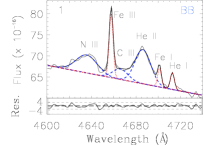
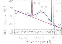
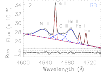
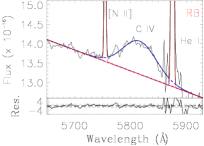
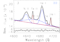
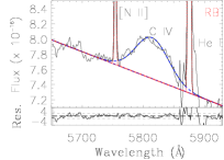
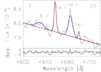
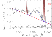
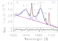
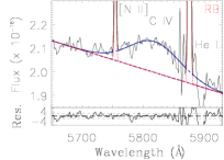
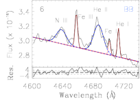
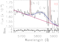
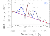
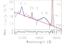
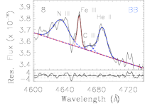
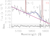
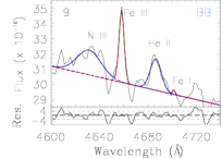
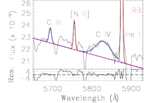
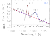
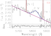
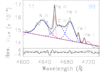
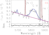
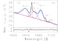
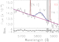
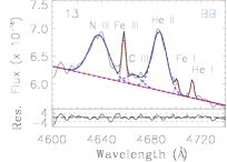
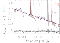
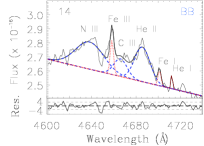
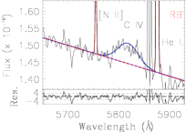
Figure 7: Multi-component Gaussian fits to the bumps of the 38 star-forming complexes with WR features in the Antennae: the blue bump (BB) (left) and the red bump (RB) (right) are fitted by their broad (dashed blue) and nebular (dotted red) lines; the sum is shown in black. The fitted continuum is shown by the dashed straight line. The spectra are identified by the numbers 1–38 and each of the fitted components is indicated. Residuals in per cent (%) are shown at the bottom of each panel. The results are listed in Table 2.

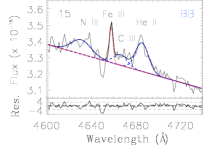
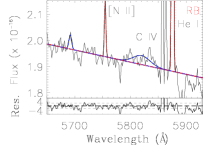
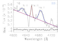
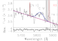
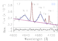
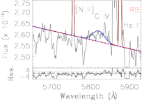
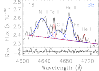
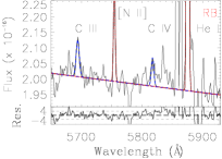
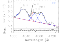
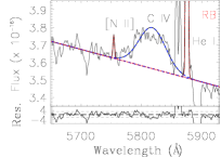
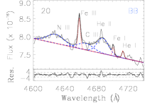
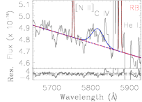
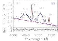
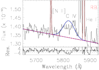
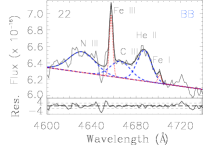
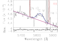
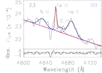
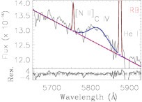
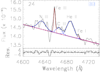
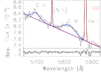
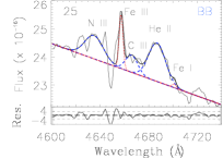
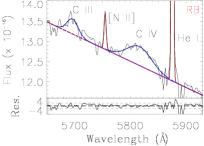
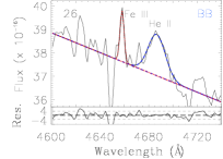
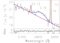
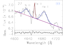
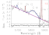
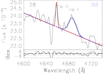
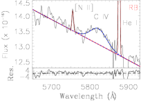
Figure 8: – continued

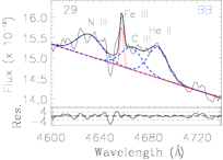
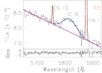
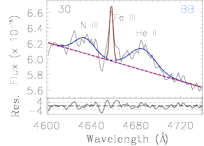
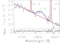
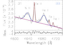
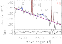
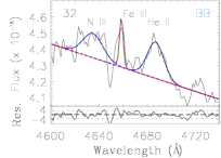
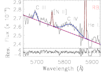
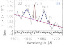
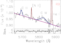
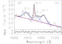
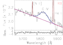
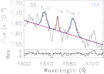
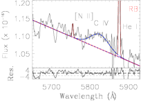
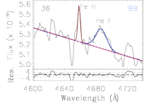
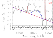
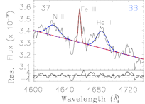
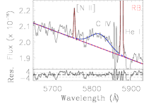
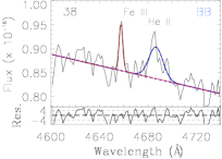
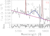
Figure 9: – continued

The multi-Gaussian fitting technique help us dissect the presence and flux from the contributing lines of the WR bumps (e.g., Brinchmann et al., 2008; López-Sánchez & Esteban, 2010; Miralles-Caballero et al., 2014; Monreal-Ibero et al., 2017; Gómez-González et al., 2020). Furthermore, it helps us to assess the contribution from contaminant nebular lines such as He i $\lambda 4713$, He ii $\lambda 4686$, and [Fe iii] $\lambda 4658$  in the BB (see, e.g., Mayya et al., 2020) and [N ii] $\lambda 5755$ and He i $\lambda 5876$ in the RB.

The BB and RB of the 38 WR spectra in the Antennae were decomposed into their individual emission lines by following the multi-Gaussian approach described in Gómez-González et al. (2020). This method consists of fitting the broad WR features with multi-Gaussian components using a tailor-made code that uses the idl routine lmfit.

Table 2: Parameters of the broad emission lines from multi-component Gaussian fitting^†.

ID |	Blue bump    |									Red bump   |
	He ii $\lambda 4686$   |			N iii $\lambda\lambda 4634,41$   |			C iii $\lambda\lambda 4647,66$   |			C iv $\lambda\lambda 5801,12$   |			C iii $\lambda 5696$   |			bumps   |		S/N
	$L$	FWHM	EW	$L$	FWHM	EW	$L$	FWHM	EW	$L$	FWHM	EW	$L$	FWHM	EW	$L_{\mathrm{BB}}$	$L_{\mathrm{RB}}$	BB	RB
(1)	(2)	(3)	(4)	(5)	(6)	(7)	(8)	(9)	(10)	(11)	(12)	(13)	(14)	(15)	(16)	(17)	(18)	(19)	(20)
1	56.0	16.6	2.5	39.5	22.3	1.7	16.5	16.1	0.7	74.2	75.6	5.3	0.0	0.0	0.0	112.0	74.2	60	127
2	20.3	16.9	2.2	19.0	25.5	2.0	12.3	20.1	1.3	25.2	70.6	4.8	0.0	0.0	0.0	51.6	25.2	48	117
3	22.3	13.0	4.4	14.0	15.6	2.6	27.9	60.6	5.3	14.3	63.6	4.8	0.0	0.0	0.0	64.1	14.3	58	93
4	2.8	9.1	1.0	1.1	15.5	0.4	0.0	0.0	0.0	6.2	58.9	3.6	0.0	0.0	0.0	3.9	6.2	56	78
5	3.4	17.7	2.7	2.8	24.5	2.1	0.9	16.4	0.7	5.3	96.4	6.6	0.0	0.0	0.0	7.1	5.3	50	95
6	2.4	14.9	2.3	1.2	15.0	1.2	0.0	0.0	0.0	2.8	82.9	4.5	0.0	0.0	0.0	3.6	2.8	68	82
7	11.0	13.2	1.0	11.5	16.0	1.0	3.1	8.3	0.3	12.7	41.7	1.8	6.1	13.6	0.8	25.6	18.8	65	52
8	1.3	12.9	1.0	1.8	22.6	1.3	0.2	10.2	0.1	1.9	64.0	2.2	0.0	0.0	0.0	3.3	1.9	64	77
9	9.3	10.7	0.9	15.9	23.2	1.4	0.0	0.0	0.0	25.6	45.0	3.0	4.0	7.8	0.4	25.2	29.6	51	46
10	1.1	15.6	0.7	0.0	0.0	0.0	0.0	0.0	0.0	1.6	48.9	1.7	0.0	0.0	0.0	1.1	1.6	55	67
11	10.1	16.6	1.9	12.3	24.5	2.3	9.3	21.4	1.8	10.6	51.8	3.0	0.7	8.8	0.2	31.7	11.3	64	103
12	14.2	16.0	1.6	16.1	25.0	1.7	11.5	18.8	1.2	10.6	47.1	2.0	0.0	0.0	0.0	41.8	10.7	54	87
13	6.3	14.1	3.0	6.0	18.9	2.7	1.0	14.1	0.5	0.0	0.0	0.0	0.0	0.0	0.0	13.3	0.0	53	77
14	1.7	16.3	1.8	2.4	29.8	2.5	0.7	14.1	0.8	1.2	47.1	2.0	0.0	0.0	0.0	4.8	1.2	53	66
15	1.0	13.7	0.9	0.8	20.8	0.6	0.4	14.1	0.3	0.5	35.3	0.7	0.1	5.5	0.2	2.2	0.6	51	74
16	1.6	14.7	0.8	0.8	14.6	0.4	0.0	0.0	0.0	2.2	47.1	1.6	0.0	0.0	0.0	2.3	2.2	66	80
17	1.7	15.7	1.4	1.2	18.2	0.9	0.0	0.0	0.0	0.7	35.3	0.7	0.0	0.0	0.0	2.9	0.7	56	77
18	1.4	12.3	1.6	1.9	21.8	2.2	0.9	18.8	1.0	0.2	4.7	0.2	0.3	6.0	0.4	4.2	0.5	58	55
19	3.6	20.6	1.7	5.7	31.7	2.7	2.7	18.8	1.3	5.1	51.8	3.6	0.0	0.0	0.0	12.0	5.1	68	75
20	3.0	16.9	1.1	2.6	24.6	0.9	1.7	22.5	0.6	2.0	35.3	1.1	0.0	0.0	0.0	7.3	2.0	59	87
21	1.5	16.1	1.9	1.5	24.2	2.0	0.9	22.5	1.1	1.9	47.1	3.7	0.0	0.0	0.0	3.9	1.9	51	62
22	2.4	15.2	1.0	2.9	27.5	1.2	1.8	21.2	0.7	3.1	47.1	1.8	0.0	0.0	0.0	7.0	3.1	74	99
23	7.9	16.3	1.0	3.8	15.8	0.4	1.9	11.8	0.2	12.7	55.0	2.5	0.0	0.0	0.0	13.7	12.7	61	87
24	5.6	15.2	1.1	3.2	16.6	0.6	1.7	11.8	0.3	5.7	51.8	1.8	2.8	32.8	0.8	10.5	8.5	63	85
25	9.4	16.4	1.1	6.2	17.7	0.7	3.0	11.8	0.4	10.0	51.0	2.0	3.6	23.6	0.7	18.6	13.6	58	78
26	12.1	16.5	0.9	0.0	0.0	0.0	0.0	0.0	0.0	19.4	65.8	2.4	0.0	0.0	0.0	12.1	19.4	52	76
27	2.7	19.4	1.1	1.6	17.5	0.6	0.0	0.0	0.0	3.3	51.9	2.3	0.4	9.0	0.2	4.3	3.7	56	83
28	6.6	15.1	0.8	0.0	0.0	0.0	0.0	0.0	0.0	10.6	49.6	2.0	0.0	0.0	0.0	6.6	10.6	56	83
29	5.9	19.1	1.1	5.4	24.2	1.0	4.6	20.6	0.8	10.0	56.2	3.1	0.0	0.0	0.0	15.9	10.0	53	92
30	3.0	26.5	1.4	1.7	20.3	0.8	0.0	0.0	0.0	2.2	48.5	1.8	0.0	0.0	0.0	4.7	2.3	59	45
31	1.4	16.9	1.8	1.0	15.0	1.2	0.0	0.0	0.0	0.6	44.0	1.2	0.1	6.3	0.2	2.4	0.7	53	70
32	1.5	16.0	1.0	1.2	19.3	0.8	0.0	0.0	0.0	2.3	55.2	2.3	0.5	13.1	0.5	2.7	2.8	55	68
33	0.5	12.0	0.9	0.5	14.7	0.8	0.0	0.0	0.0	0.6	41.5	1.5	0.2	10.8	0.5	1.0	0.8	52	61
34	1.3	18.1	1.1	1.2	21.0	1.0	0.8	17.4	0.7	2.6	53.3	3.2	0.0	0.0	0.0	3.2	2.6	58	82
35	0.4	10.9	0.6	0.3	9.6	0.5	0.0	0.0	0.0	0.9	54.2	2.2	0.0	0.0	0.0	0.7	0.9	60	56
36	1.3	16.2	0.7	0.0	0.0	0.0	0.0	0.0	0.0	3.9	55.1	2.7	0.0	0.0	0.0	1.3	3.0	63	77
37	0.9	15.4	0.8	0.6	17.4	0.5	0.0	0.0	0.0	2.0	56.2	2.6	0.0	0.0	0.0	1.6	2.0	58	66
38	0.4	13.6	1.2	0.0	0.0	0.	0.0	0.0	0.0	0.9	53.2	3.8	0.0	0.0	0.0	0.4	0.9	48	47

Notes. Brief explanation of columns: (1) WR identification; (2) luminosity of He ii $\lambda 4686$ [$1.0\times 10^{37}$ erg s^-1] at a distance of 18.1 Mpc; (3) full width at half maximum (FWHM) [Å]; (4) equivalent width (EW) [Å]; (5) luminosity [$1.0\times 10^{37}$ erg s^-1], (6) FWHM [Å] and (7) EW [Å] of N iii $\lambda\lambda 4634,41$; (8) luminosity [$1.0\times 10^{37}$ erg s^-1], (9) FWHM [Å] and (10) EW [Å] of C iii $\lambda\lambda 4647,66$; (11) luminosity [$1.0\times 10^{37}$ erg s^-1], (12) FWHM [Å] and (13) EW [Å] of C iv $\lambda\lambda 5801,12$; (14) luminosity [$1.0\times 10^{37}$ erg s^-1], (15) FWHM [Å] and (16) EW [Å] of C iii $\lambda 5696$; (17) BB luminosity ($L_{\rm BB}$) [$1.0\times 10^{37}$ erg s^-1]; (18) RB luminosity ($L_{\rm RB}$) [$1.0\times 10^{37}$ erg s^-1]; (19) continuum BB signal-to-noise ratio (S/N_BB) at 4750–4830 Å; (20) S/N_RB at 5650–5730 Å. ^†The multi-Gaussian fittings are shown in Fig. 7.

Table 3: Parameters of the nebular emission lines.

ID	$\mathrm{log}F$(H$\beta$)	EW(H$\beta$)	EW(H$\alpha$)	$A_{\mathrm{V}}$	$T_{\mathrm{e}}$([N ii])	$T_{\mathrm{e}}$([S iii])	$n_{\rm e}$([Cl iii])	$n_{\rm e}$([S ii])	$\mathrm{12+log(O/H)}$		$V_{\mathrm{r}}$
	(erg cm-2 s-1)	(Å)	(Å)	(mag)	($\times 10^{3}$ K)	($\times 10^{3}$ K)	(cm-3)	(cm-3)	DR	R3	( km s-1)
(1)	(2)	(3)	(4)	(5)	(6)	(7)	(8)	(9)	(10)	(11)	(12)
1	$\mathrm{-12.574}\pm$0.001	83.9	415.7	0.70$\pm$0.01	7.96$\pm$0.08	7.40$\pm$0.04	200$\pm$290	229.8$\pm$2.9	9.01$\pm$0.02	8.50$\pm$0.01	1468.0$\pm$5.7
2	$\mathrm{-12.721}\pm$0.001	121.2	684.5	0.66$\pm$0.01	8.37$\pm$0.07	8.02$\pm$0.05	$\cdots$	191.4$\pm$1.9	8.81$\pm$0.01	8.50$\pm$0.01	1433.0$\pm$5.9
3	$\mathrm{-12.854}\pm$0.001	139.1	831.2	0.81$\pm$0.01	8.60$\pm$0.09	8.30$\pm$0.03	240$\pm$150	81.0$\pm$1.8	8.60$\pm$0.03	8.50$\pm$0.01	1452.7$\pm$2.9
4	$\mathrm{-13.563}\pm$0.004	54.5	278.8	0.96$\pm$0.01	8.10$\pm$0.40	8.80$\pm$0.40	$\cdots$	74.6$\pm$1.6	8.62$\pm$0.09	8.67$\pm$0.01	1491.7$\pm$4.0
5	$\mathrm{-13.393}\pm$0.001	112.8	658.1	1.13$\pm$0.01	8.47$\pm$0.23	8.56$\pm$0.10	500$\pm$700	60.1$\pm$2.0	8.65$\pm$0.05	8.56$\pm$0.01	1449.6$\pm$5.0
6	$\mathrm{-13.445}\pm$0.002	150.6	846.5	0.96$\pm$0.01	8.27$\pm$0.16	8.19$\pm$0.10	$\cdots$	51.4$\pm$1.1	8.65$\pm$0.04	8.57$\pm$0.01	1452.4$\pm$3.6
7	$\mathrm{-12.924}\pm$0.004	27.9	183.1	1.20$\pm$0.01	6.70$\pm$0.70	5.30$\pm$1.00	$\cdots$	134.8$\pm$3.0	8.70$\pm$0.70	$\cdots$	1632.4$\pm$3.6
8	$\mathrm{-13.548}\pm$0.004	44.7	285.8	0.97$\pm$0.01	7.15$\pm$0.32	6.40$\pm$0.50	$\cdots$	57.5$\pm$0.6	8.90$\pm$0.11	8.97$\pm$0.01	1544.1$\pm$3.8
9	$\mathrm{-12.665}\pm$0.006	39.7	220.0	2.57$\pm$0.02	8.00$\pm$0.50	7.20$\pm$0.80	$\cdots$	387.0$\pm$22	8.58$\pm$0.13	9.11$\pm$0.01	1710.8$\pm$9.5
10	$\mathrm{-13.764}\pm$0.006	33.6	206.4	0.77$\pm$0.02	7.00$\pm$0.50	6.20$\pm$0.50	$\cdots$	70.0$\pm$4.0	9.01$\pm$0.12	8.91$\pm$0.01	1555.0$\pm$2.2
11	$\mathrm{-12.756}\pm$0.002	67.1	434.9	1.29$\pm$0.01	7.62$\pm$0.18	7.07$\pm$0.22	$\cdots$	64.7$\pm$0.6	8.81$\pm$0.05	8.83$\pm$0.01	1581.5$\pm$4.3
12	$\mathrm{-12.942}\pm$0.003	48.9	316.5	0.69$\pm$0.01	7.48$\pm$0.16	7.16$\pm$0.29	$\cdots$	56.6$\pm$1.2	8.86$\pm$0.05	8.87$\pm$0.01	1616.9$\pm$0.9
13	$\mathrm{-13.225}\pm$0.001	98.0	666.6	0.79$\pm$0.01	7.55$\pm$0.13	7.58$\pm$0.08	$\cdots$	67.0$\pm$4.0	8.87$\pm$0.06	8.77$\pm$0.01	1644.5$\pm$4.1
14	$\mathrm{-13.764}\pm$0.003	65.0	400.8	0.79$\pm$0.01	7.36$\pm$0.30	7.81$\pm$0.35	$\cdots$	48.3$\pm$0.1	8.92$\pm$0.05	8.88$\pm$0.01	1629.3$\pm$6.8
15	$\mathrm{-13.822}\pm$0.004	37.5	230.9	0.95$\pm$0.01	7.80$\pm$0.40	7.70$\pm$0.60	300$\pm$700	24.0$\pm$1.6	8.81$\pm$0.10	8.81$\pm$0.01	1634.0$\pm$4.8
16	$\mathrm{-13.693}\pm$0.007	23.0	131.8	0.93$\pm$0.02	7.30$\pm$0.80	6.10$\pm$3.50	$\cdots$	22.4$\pm$3.0	8.95$\pm$0.32	8.94$\pm$0.01	1652.7$\pm$3.8
17	$\mathrm{-12.938}\pm$0.003	109.3	635.6	1.50$\pm$0.01	7.96$\pm$0.20	7.66$\pm$0.15	$\cdots$	87.2$\pm$2.7	8.83$\pm$0.04	8.65$\pm$0.01	1570.8$\pm$4.2
18	$\mathrm{-13.001}\pm$0.003	75.4	511.5	2.67$\pm$0.01	6.99$\pm$0.26	6.70$\pm$1.10	$\cdots$	75.2$\pm$1.6	8.92$\pm$0.16	$\cdots$	1607.2$\pm$4.6
19	$\mathrm{-13.800}\pm$0.008	21.9	125.6	0.70$\pm$0.02	8.90$\pm$0.70	6.40$\pm$1.10	$\cdots$	25.6$\pm$2.0	8.61$\pm$0.17	8.67$\pm$0.01	1580.6$\pm$2.4
20	$\mathrm{-13.305}\pm$0.004	53.4	309.8	1.08$\pm$0.01	8.10$\pm$0.50	8.00$\pm$0.60	$\cdots$	28.0$\pm$4.0	8.82$\pm$0.16	8.58$\pm$0.01	1467.8$\pm$1.7
21	$\mathrm{-13.617}\pm$0.003	102.7	546.0	1.00$\pm$0.01	8.30$\pm$0.28	8.07$\pm$0.30	100$\pm$600	73.2$\pm$2.4	8.83$\pm$0.05	8.61$\pm$0.01	1488.1$\pm$4.6
22	$\mathrm{-12.994}\pm$0.004	44.0	313.4	1.87$\pm$0.01	7.20$\pm$0.40	6.60$\pm$0.50	$\cdots$	83.0$\pm$6.0	8.92$\pm$0.14	8.95$\pm$0.01	1583.3$\pm$3.7
23	$\mathrm{-12.989}\pm$0.005	31.4	215.5	1.27$\pm$0.01	7.40$\pm$0.60	6.60$\pm$0.80	$\cdots$	59.0$\pm$7.0	8.68$\pm$0.27	9.05$\pm$0.01	1650.8$\pm$4.7
24	$\mathrm{-12.989}\pm$0.003	46.9	336.1	0.96$\pm$0.01	6.87$\pm$0.29	6.31$\pm$0.27	$\cdots$	79.9$\pm$0.7	8.83$\pm$0.16	9.13$\pm$0.01	1655.6$\pm$4.4
25	$\mathrm{-12.983}\pm$0.004	32.5	234.5	0.86$\pm$0.01	7.40$\pm$0.50	6.20$\pm$0.60	$\cdots$	60.1$\pm$2.6	8.55$\pm$0.29	9.15$\pm$0.01	1626.8$\pm$5.2
26	$\mathrm{-12.944}\pm$0.007	16.9	132.8	1.16$\pm$0.02	8.30$\pm$0.70	6.70$\pm$0.90	$\cdots$	80.0$\pm$7.0	8.43$\pm$0.28	8.92$\pm$0.01	1608.7$\pm$3.8
27	$\mathrm{-13.693}\pm$0.005	26.6	173.1	0.78$\pm$0.01	7.20$\pm$0.60	5.90$\pm$3.40	$\cdots$	37.0$\pm$4.0	8.70$\pm$0.50	9.08$\pm$0.01	1593.7$\pm$6.0
28	$\mathrm{-13.047}\pm$0.006	27.0	178.4	1.12$\pm$0.01	7.40$\pm$0.70	6.00$\pm$4.00	$\cdots$	60.0$\pm$5.0	8.60$\pm$0.40	9.10$\pm$0.01	1574.4$\pm$4.5
29	$\mathrm{-13.344}\pm$0.004	27.4	183.2	1.05$\pm$0.01	8.00$\pm$0.60	6.80$\pm$0.60	$\cdots$	40.5$\pm$0.9	8.51$\pm$0.19	8.93$\pm$0.01	1664.1$\pm$2.0
30	$\mathrm{-13.465}\pm$0.003	47.6	329.6	1.09$\pm$0.01	7.53$\pm$0.24	7.04$\pm$0.32	$\cdots$	55.1$\pm$2.4	8.75$\pm$0.08	8.95$\pm$0.01	1690.8$\pm$8.7
31	$\mathrm{-13.445}\pm$0.001	100.5	695.0	1.29$\pm$0.01	6.90$\pm$0.11	6.50$\pm$0.13	1800$\pm$1800	219.0$\pm$2.8	9.06$\pm$0.03	9.05$\pm$0.01	1675.9$\pm$5.7
32	$\mathrm{-13.603}\pm$0.005	28.1	201.8	1.56$\pm$0.01	7.80$\pm$0.60	5.60$\pm$3.20	$\cdots$	64.7$\pm$2.1	8.40$\pm$0.70	$\cdots$	1632.2$\pm$1.6
33	$\mathrm{-13.868}\pm$0.004	47.5	315.4	1.42$\pm$0.01	6.60$\pm$0.50	5.00$\pm$3.00	$\cdots$	91.0$\pm$8.0	8.80$\pm$0.60	$\cdots$	1676.9$\pm$5.8
34	$\mathrm{-13.651}\pm$0.005	28.4	204.7	1.69$\pm$0.01	7.50$\pm$0.70	6.30$\pm$0.90	$\cdots$	41.0$\pm$4.0	8.67$\pm$0.25	9.01$\pm$0.01	1691.2$\pm$3.8
35	$\mathrm{-14.120}\pm$0.009	24.0	146.5	1.46$\pm$0.02	7.60$\pm$1.00	6.50$\pm$1.50	$\cdots$	67.0$\pm$7.0	8.10$\pm$2.90	$\cdots$	1674.1$\pm$14.6
36	$\mathrm{-13.706}\pm$0.009	17.9	102.8	1.16$\pm$0.02	9.20$\pm$1.30	7.40$\pm$1.40	100$\pm$400	49.0$\pm$13	8.20$\pm$0.50	8.81$\pm$0.01	1547.1$\pm$4.3
37	$\mathrm{-13.878}\pm$0.005	38.3	215.0	0.97$\pm$0.01	7.90$\pm$0.50	7.00$\pm$0.70	$\cdots$	26.7$\pm$3.5	8.60$\pm$0.17	8.96$\pm$0.01	1672.6$\pm$4.5
38	$\mathrm{-13.947}\pm$0.007	50.2	330.2	1.78$\pm$0.02	8.20$\pm$0.60	7.40$\pm$0.60	$\cdots$	28.0$\pm$13	8.60$\pm$0.50	8.77$\pm$0.01	1694.5$\pm$3.2

Notes. Brief explanation of columns: (1) WR identification (1–38); (2) ^†reddening-corrected fluxes of $\mathrm{log}F$(H$\beta$) [erg cm^-2 s^-1]; (3) equivalent width (EW) of H$\beta$ [Å]; (4) EW of H$\alpha$ [Å]; (5) visual extinction ($A_{\rm V}$) [mag]; (6) electron temperature ($T_{\mathrm{e}}$) of the low-ionization zone ([N ii]) [K]; (7) $T_{\mathrm{e}}$ of the medium-ionization zone ([S iii]) [K]; (8) electron density ($n_{\rm e}$) from [Cl iii] [cm³]; (9) $n_{\rm e}$([S ii]) [cm³]; (10) R3-oxygen abundance; (11) Direct method (DM)-oxygen abundance; (12) radial velocity ($V_{\mathrm{r}}$) [ km s^-1].

We were able to decompose the BB into He ii, N iii and C iii broad emission lines, while the C iii and C iv broad emission lines were used for the RB. C iii $\lambda 5696$ clearly indicates WCL presence, whilst if there is only C iv $\lambda\lambda 5801,12$ it suggests WCE-subtypes. N iii $\lambda\lambda 4634,41$ in the BB is a WNL component. To avoid any contamination from narrow-nebular lines, we also fitted the [Fe i], [Fe iii] and He i in the BB and the [N ii] and He i in the RB. This approach independently confirms what was obtained through Galactic templates, with the benefit of also having determined the parameters of the emission features contributing to the WR bumps. Details of the estimated fluxes, EWs and FWHMs are listed in Table 2 and the fits are illustrated in Fig. 7 for all WR spectra.

3.3 Physical properties of the WR environments

The rest of the nebular lines of the spectra were analysed following iraf standard routines (Tody, 1993) and were corrected for extinction by using the $c$(H$\beta$) value estimated from the Balmer decrement method. We assume an intrinsic Balmer decrement ratio corresponding to a case B photoionised nebula with electron temperature ($T_{\mathrm{e}}$) = 10000 K and the electron density ($n_{\mathrm{e}}$) = 100 cm^-3 (see Osterbrock & Ferland, 2006) and the reddening curve of Cardelli et al. (1989). Reddening-corrected line fluxes for different nebular lines used to determine the physical conditions in the ionized zones of the 38 WR spectra are presented in Table 5, in the Appendix C.

3.3.1 Oxygen chemical abundance

We calculated oxygen chemical abundance using the direct method (DM). This implies that the determined oxygen abundance depends on the physical conditions in the gas: $T_{\mathrm{e}}$ and $n_{\mathrm{e}}$.

We need $T_{\mathrm{e}}$ for the low and medium ionization zones to estimate the ionic $\rm{O^{+}}$ and $\rm{O^{++}}$ abundances. We used $T_{\mathrm{e}}$([N ii]) as the temperature for the low ionization region. Due to the fact that MUSE does not observe the blue part of the spectra where [O iii] $\lambda 4363$ resides, we cannot determine $T_{\mathrm{e}}$([O iii]). We use instead the $T_{\mathrm{e}}$([S iii]) for the medium ionization region, which has been proven to be reliable (Berg et al., 2015; James et al., 2020).

$T_{\mathrm{e}}$([N ii]) and $n_{\rm e}$([S ii]) were calculated simultaneously using PyNEB (Luridiana et al., 2015) and the [N ii]: I($\lambda 6548$+$\lambda 6584$)/I($\lambda 5755$) and [S ii]: I($\lambda 6717$)/I($\lambda 6731$) diagnostics, respectively. We also used PyNEB to determine simultaneously $T_{\mathrm{e}}$([S iii]) and $n_{\rm e}$([S ii]) using the [S iii]: I($\lambda 6312$)/I($\lambda 9069$) and [S ii] diagnostics, respectively. For the few regions where [Cl iii]$\rm{\lambda 5517/\lambda 5537}$ were detected, $n_{\rm e}$([Cl iii]) was also determined simultaneously with $T_{\mathrm{e}}$([N ii]). We estimated the uncertainties propagating the relative error of the line fluxes to the PyNEB determinations. For those regions where [S iii] was not detected, we estimated $T_{\mathrm{e}}$([S iii]) for the medium ionization zone using the relations from Garnett (1992):

$$T_{\rm{e}}^{\rm{low}}=0.7\thinspace T_{\rm{e}}^{\rm{medium}}+3000\thinspace\rm{K}$$ (2)

Ionic abundances were estimated using PyNEB, where we used as inputs the $T_{\rm{e}}$ corresponding to each ionization zone, the $n_{\rm e}$([S ii]) estimated previously, as well as the [O ii] $\lambda 7320$ and [O ii] $\lambda 7330$ lines for the $\rm{O^{+}}$ ion, while [O iii] $\lambda 4959$ and [O iii] $\lambda 5007$ lines for the $\rm{O^{2+}}$ ion. The relative uncertainty of the ionic abundance for each line is determined from the quadratic sum of the relative $T_{\rm{e}}$, $n_{\rm{e}}$, and flux ratios uncertainties. The ionic abundances are obtained by an error-weighted average of the ionic abundance for each line. Finally, we sum both ionic abundances to obtain the total oxygen abundance.

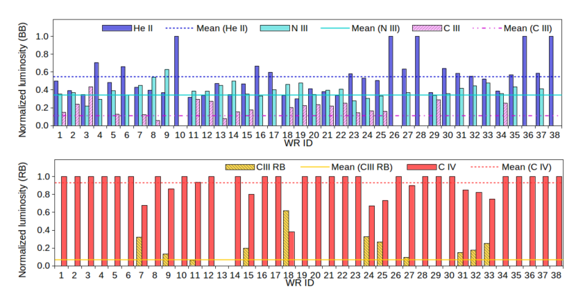
Figure 10: (top) The contribution from each WR broad component to the total luminosity of the BB feature, $L\mathrm{(BB)}$. He ii is the dominating emission line, followed by C iii and N iii with averaged values of $\sim$55%, $\sim$35% and $\sim$10% of the total $L$(BB), respectively. (bottom) The contribution of the C iii  and C iv emission lines to the RB luminosity, $L\mathrm{(RB)}$. On average, the C iv  contributes to $>$85% of $L\mathrm{(RB)}$. The multi-Gaussian fittings are presented in Fig. 7 and the results listed in Table 2.

For comparison, we also calculate the oxygen abundance in the emission-line regions using the observational R3 relation (following Vacca & Conti, 1992; Bastian et al., 2006)

$$\mathrm{log(O/H)=-0.69\,log\,R_{3}-3.24},$$ (3)

where $R_{\mathrm{3}}$ is defined as

$$R_{3}=\frac{I(\mathrm{O\,III~{}4959})+I(\mathrm{O\,III~{}5007})}{I(\mathrm{H}\beta)}$$ (4)

which is valid for $-0.6\leq\ \mathrm{log}\,R_{\mathrm{3}}\leq\ 1.0$.

We summarize the results in Table 3. The mean oxygen abundance resulted in $\mathrm{12+log(O/H)}\approx 8.9$, which is practically Solar metallicity ($Z=0.02$). As a reference, the Solar metallicity given by Asplund et al. (2009) is 12+log(O/H)=8.69 (Z=0.014).

3.3.2 Kinematic information

We considered the observed wavelengths of the [O iii] $\lambda 5007$, H$\beta$ and H$\alpha$ lines, which have the highest signal-to-noise ratio, to determine the radial velocities of the different SSCs with WR features. The spectral resolution of the observations was high enough to enable us to also obtain information about the kinematics. Table 3 lists the radial velocities for the nebular environment of each WR SSC, ranging from 1430 to 1700  km s^-1, which is in excellent agreement with previous kinematical studies (e.g., Bastian et al., 2006). According to NASA/NED, the heliocentric velocity for NGC 4038 is 1642$\pm$12  km s^-1.

4 Discussion

The entire sample of WR stars we report in the Antennae are hosted in H ii regions, however, not all the H ii regions in these galaxies harbour WR stars. For example, the smallest and southernmost galaxy, NGC 4039, does not exhibit any hint of WR features. Furthermore, data cubes covering the field in the outskirts of the Antennae were found to have intermediate ages (100–300 Myr) in Whitmore et al. (2010), therefore, it is not rare for it not to have WR stars.

Notice that the physical sizes of the complexes found to harbour WR stars in the Antennae galaxies are quite large (see Table 1), with diameters between $\sim 100-350$ pc, which are comparable to the size of the Tarantula in the LMC ($\sim 300$ pc; see Crowther, 2019).

Extragalactic WR stars are mostly detected at the location of H ii complexes, generally tracing the spiral arms of the galaxies. This is also the case for the Antennae, particularly for NGC 4038, the northern and larger of this pair of galaxies (see Fig. 1). The distribution of star-forming regions in figure 19 of Gunawardhana et al. (2019) confirms that all the WR features reported in the present work concur with very young H ii regions with ages $\lesssim$4 Myr.

Interestingly, WR 1, the SSC complex with the strongest WR features, and therefore the largest number of estimated WR stars (800 WR), is located at the bridge between these merging galaxies. It also has the strongest hydrogen lines in emission (see below).

We estimated a total of 4053 $\pm$ 84 WR stars in the Antennae galaxies, which is among the highest number reported in the literature of galaxies harbouring such stars. Even if we adopt a foreground Galactic extinction $A_{\rm V}$=0.127 mag (Schlafly & Finkbeiner, 2011) as a lower limit for the quantification of WR stars, the number would be $\sim 2000$ WR stars. On the other hand, if we consider a greater distance to the Antennae, for example the 22 Mpc estimated by Schweizer et al. (2008) based on the type Ia supernova 2007sr, the total number of WR stars would raise by $\sim$48%, given a higher intrinsic luminosity of their WR bumps.

Through the detailed multi-Gaussian decomposition presented in Section 3, we were able to avoid any contamination from nebular emission lines and evaluate the contribution from each broad emission line to the entire luminosity of both WR features. On average, the He ii emission line corresponds to $\sim$55% of the BB luminosity ($L\mathrm{(BB)}$), followed by C iii and N iii with $\sim$35% and $\sim$10%, respectively. This is illustrated in Fig. 10 top panel.

In particular, for WR 10, 26, 28, 36 and 38, their BB is constituted only by He ii, even though these are classified as WCE-subtypes. We recall that this classification comes from their RB feature. It does not mean that there is no carbon in the BB, but rather that it is probably not intense enough and therefore unresolved by our analysis. Thus, one must be careful to rule out the presence of WC-types in those cases in which the BB is dominated by He ii. The RB is determinant for any classification. By definition C iii is not present in WCE-subtypes. C iv clearly dominates the RB luminosity ($L$(RB)) contributing with $>$85% to the total in WCL-subtypes (see Fig. 10 bottom panel).

We do not find any evidence of the nebular He ii emission line with the multi-Gaussian fitting decomposition, apparently only common in metal-poor environments ($\mathrm{12+log(O/H)}\leq 8.4$; see, e.g., Kehrig et al., 2011, 2018). Thus, we do not need to invoke other sources of hard ionizing radiation (see, e.g., figure 1 in Schaerer et al., 2019, it is expected that higher the metallicity, lower the intensity of nebular He ii emission line).

In Fig. 11 we illustrate the $L$(BB) vs. $L$(RB) relation for the 38 WR spectra. This figure shows that there is a trend, with higher $L$(BB) corresponding to higher $L$(RB). Furthermore, since the total H$\beta$ luminosity, $L$(H$\beta$), can be roughly associated with the population of ionizing O-type stars, we show in Fig. 12 the relation between $L$(BB) and $L$(H$\beta$). This figure shows that those clusters with the highest number of WR stars also show the highest values in the luminosities of H$\beta$, which is not unexpected since WR stars are considered descendants of O-type stars. We note that WR 1 is located in the most luminous regions in both figures.

Figure 11: $L\mathrm{(BB)}$ vs. $L\mathrm{(RB)}$ relation of the 38 WR SSC complexes in the Antennae. For reference, the red symbol corresponds to WR 1, the one with the highest luminosities in its bumps.

Figure 12: $L$(H$\beta$) vs. $L$(BB) for the 38 WR SSC complexes in the Antennae. The red symbol corresponds to WR 1, the one with the highest L(H$\beta$), correlated with number of O-type stars.

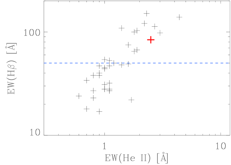
Figure 13: EW(H$\beta$) vs. EW(He ii) for the 38 WR SSC complexes in the Antennae. The red symbol corresponds to WR 1, with one of the highest EW(H$\beta$), related to the age of the starburst, and also one of the highest EW(He ii). EW(H$\beta$)$>$50 Å, above the blue dashed line, suggest a starburst age $\leq$5 Myr.

The EW of the H$\beta$ emission lines can be used to assess the age of young starbursts. In Fig. 13 we show the EW of H$\beta$ versus the EW of He ii for the 38 WR SSC complexes in the Antennae. It has been suggested that an EW(H$\beta$)$>$50 Å corresponds to starburst ages $\leq$5 Myr (see, e.g. Chávez et al., 2016). Many of our objects are above this value, suggesting an even younger stellar population. Our diagram shows that the greater the EW(H$\beta$), the stronger the intensity of the He ii, also meaning more WR stars. However, it is important to emphasize that, although all the WR stars in the Antennae are hosted in H ii regions, not all the detected H ii regions harbour WR stars.

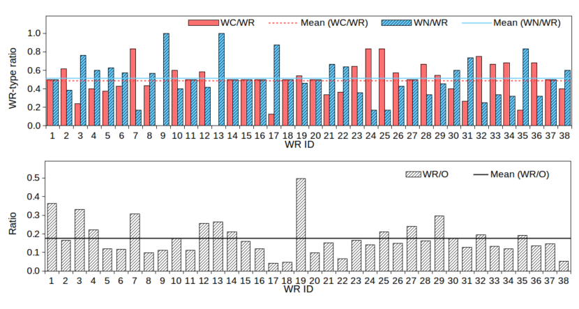
Figure 14: (top) Histogram of WC/WR (red) and WN/WR (blue) ratios of WR stars; (bottom) WR/O ratio of stars.

Reviewing the literature of the so-called WR galaxies, there is a consensus in the massive stars community that a high-metallicity favours WC-type stars and its later subtypes (WCE, WCL and WO), which are otherwise rare in low-metallicity galaxies. As previously discussed, given the wavelength range of our spectra, we cannot inquire whether or not there are any WO-type stars present. However, any WO-type stars would be already included in the WC-type stars count since they, too, do display the RB feature. Spectrographs equipped with Integral Filed Units (IFU) such as MEGARA at the GTC covering the blue spectral range are essential to unveil the O-rich WR population, little studied or observed at extragalactic distances.

Of the total number of WR stars found in the Antennae, half correspond to WN-types, and the other half are WC-types (see Fig. 14, top panel). The global WC/WN ratio in the Antennae is thus $\sim$1 (see Fig. 15 top panel). It is interesting to note in Table 1 that we observe the highest local WC/WN ratios when WCL-subtypes are present. There are only two zones which have WNL stars, solely, the rest correspond to WR cluster complexes with a combination of WNL, WCE or WCL-subtypes. WNE templates were not needed in any region studied. It is reasonable to discard this population given that neither was N v observed in the BB after a careful multi-Gaussian fitting (see Fig. 7 and Table 2).

The averaged fraction of WR stars over the number of O-type stars in the Antennae is $\sim$20 per cent, which is the value obtained for the majority of the regions studied (see Fig. 14, bottom panel). Nevertheless, Eldridge et al. (2017) warns us that "one problem with such comparisons is uncertainty in how complete each observational sample is, especially for the WR/O ratio where both stellar types are hot and difficult to find in optical surveys." Our determination of the global number of O-type stars is necessarily incomplete considering that we have only taken into account those in clusters where WR features were found. Increasing the number of O-type stars, which is to be expected, the WR/O ratio will decrease, so our estimate represents an upper limit (see Fig. 15 bottom).

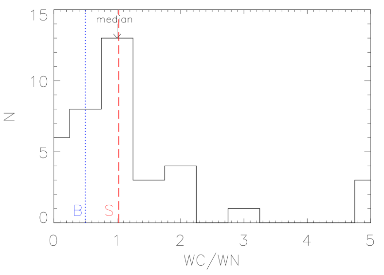
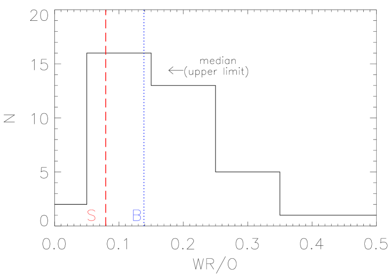
Figure 15: (top) WC/WN ratio. Median value $\sim$1 is indicated with an arrow. (bottom) WR/O ratio. An upper limit for the median value $\sim$0.2 is indicated with an arrow. Vertical blue dotted and red dashed lines indicate predicted values from BPASS binary and single models, respectively, in both panels.

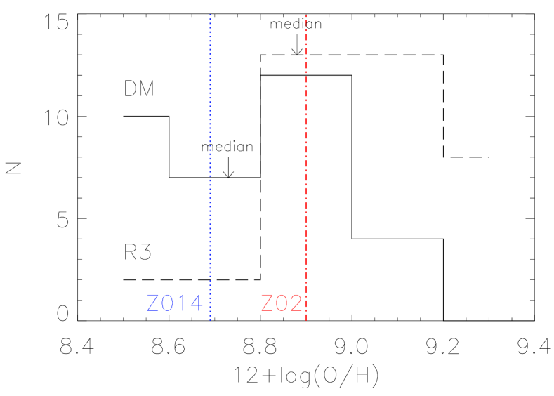
Figure 16: Histograms of the oxygen abundances determined with the R3 (dashed line) a DM (solid line) methods. Median values $\sim$8.7 and $\sim$8.9, for the R3 and DM method, are indicated with an arrow. As a reference, metallicity Z=0.014 (Solar) and Z=0.02, are indicated by a vertical blue dotted and red dotted-dashed lines, respectively.

In Fig. 16 we show that the metallicity of the Antennae corresponds with values around Solar, with and oxygen abundance $\mathrm{12+log(O/H)}\approx 8.9$. At this metallicity, the WC/WN ratio is expected to be $\sim$0.5 and $\sim$1, for binary and single stars, respectively (see Fig. 15 top panel), according to the current Binary Population and Spectral Synthesis (BPASS v2.2.1) models by Eldridge et al. (2017).

In Fig. 17 we show the BPASS models for the WC/WN and WR/O ratios vs. oxygen abundance to compare with our estimations for the Antennae. This has been illustrated in Monreal-Ibero et al. (2017) and Neugent & Massey (2019) for several galaxies with different metallicities. The global WC/WN ratio for the Antennae is in agreement with a population of single stars, not unusual since at Solar metallicity, the effect of binaries is expected to be small. On the other hand, if one assumes that each SSC complex with WR stars represents an independent zone of star formation, the local WR/O ratios should to be taken account. There are 7 cases with WC/WN ratios $\lesssim$0.5: WR 3, 9, 13, 17, 21, 31 and 35 (see Table 1), corresponding to those with the highest WN/WR ratios in Fig. 14 top panel. In these WR complexes, WN-types dominate over WC-types by $\times$2, in accordance with the binary scenario (see Fig. 15 top panel). Several studies in the literature consider global WC/WN and WR/O ratios (see e.g Monreal-Ibero et al., 2017, and references therein), or at specific galactocentric zones when there is a metallicity gradient (e.g., Rosslowe & Crowther, 2015). This is not a trivial issue for the Antennae, seeing that it is actually a pair of merging galaxies and thus any galactocentric parameter may not be relevant.

Finally, the template-fitting method has been used in several works to classify WR stars (e.g., Hadfield & Crowther, 2006, 2007; Kehrig et al., 2013; Gómez-González et al., 2020). However, it is still not clear how representative a template spectrum is for a given subtype. That is, what is the dispersion in the strengths of different lines in the individual spectra used for obtaining the template. An in-depth study of line strengths of WR stars in the Galaxy updated with new astrometric and photometric information from Gaia would be required to address this question.

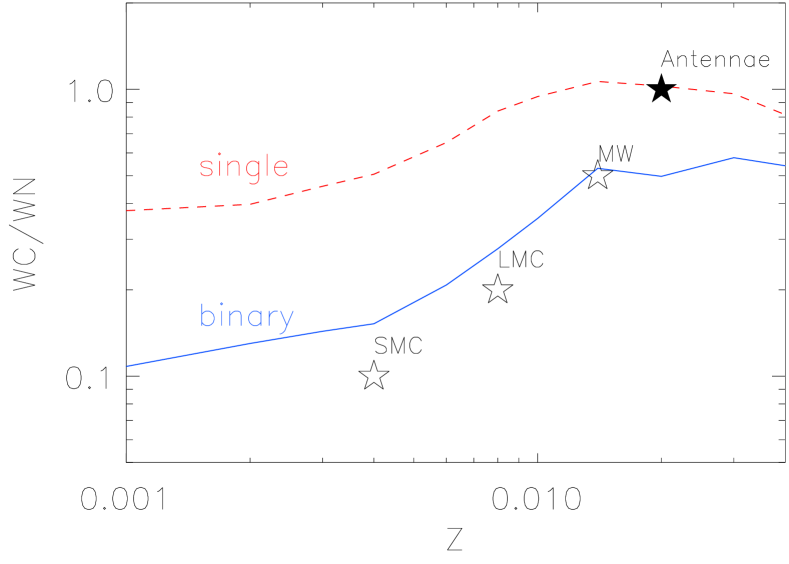
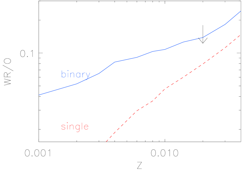
Figure 17: (top) WC/WN vs. metallicity. Blue lines correspond to BPASS binary models and red dashed lines the single models. The black star shows the averaged WC/WN estimation for the Antennae. For comparison, we also show the values for the Magellanic Clouds and the Milky Way taken from Rosslowe & Crowther (2015), shown with open stars. (bottom) WR/O vs. metallicity. The upside down arrow represents an upper limit for the Antennae, since we only computed the number of O-type stars in the SSCs with WR stars.

5 SUMMARY AND CONCLUDING REMARKS

We have used VLT MUSE data cubes from the ESO archive to search for WR stars in star-forming complexes of the Antennae galaxies. We reported their number, classification and distribution. Our results can be summarized as follows.

• We detected 38 WR SSC complexes with 4053 $\pm$ 84 WR stars, out of which 2021 $\pm$ 60 are WNL, 2032 $\pm$ 59  WC-types. We cannot uncover a plausible presence of WO-type stars given the limited spectral range covered by the observations used for this study. Further observations that covering the VB could confirm or rule out this population, the rarest type of WR stars. However, thanks to the GTC spectrum of WR 1, we can rule out the presence of WO-type stars in this SSC complex, the one with the highest number of WR stars in the Antennae.

• Galactic WR templates of WNL, WCE and WCL-subtypes were appropriate to classify and quantify the WR stars of each SSC complex, given the metallicity of the Antennae, with an oxygen abundance $\mathrm{12+log(O/H)}\approx 8.9$.

• We analysed the observed WR blue and red bumps using multiple-component Gaussian fitting in order to recover the ionic transitions responsible for the bumps and report their main parameters. In all cases, the recovered ions are consistent with those expected for the inferred subtype using the templates. Avoiding any nebular contamination, we evaluated the contribution for each broad emission line to the entire luminosity of the BB and the RB of the entire WR sample. We do not find any evidence of the nebular He ii emission line. This is explained by theoretical models, as discussed, given the high metallicity of the Antennae.

• We estimated the main physical properties of the WR nebular environments, oxygen abundances, and presented information regarding their kinematics.

• We derive a global WC/WN ratio $\sim$1, which, according to predictions of the current BPASS models is consistent with the single-star scenario, not unusual considering the Solar metallicity of the Antennae. We determined the number of O-type stars in the SSC complexes with WR features and estimated a global WR/O ratio around 20 per cent.

• With this work, Antennae has one of the largest number of WR stars recorded in the literature. The detection of this number of WR stars in the Antennae increases the sample of extragalactic WR stars, SNIbc candidates and other post-SN by-products.

Data availability

The data underlying this work are available in the article. All the observations are in the public domain. The links and observation IDs are available in the article. The reduced OSIRIS files will be shared on request to the first author.

Appendix A VLT MUSE observations

Fig. 18 shows the FoV of the 23 datasets of the Antennae obtained with the VLT MUSE instrument. The left panel shows all available observations whilst the right panel shows only the four data cubes that include the contribution of WR features. These are the data used in the present work. Details of these four observations are listed in Table 4.

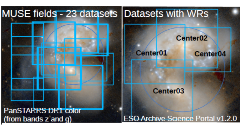
Figure 18: Publicly available VLT MUSE fields from ESO Science Archive Facility. (left) A total of 23 datasets of observations cover the entire galaxies. (right) The FoV of the four data cubes used in the present work.

Table 4: Details of the MUSE datasets^† in the Antennae.

Pointing	Archive ID	OB ID	Coordinates (J2000)		Date of observation		FoV	Exposure
			R.A.	Dec.	start	end	(arcmin)	time (s)
(1)	(2)	(3)	(4)	(5)	(6)	(7)	(8)	(9)
Center01	ADP.2017-03-28T13:08:20.713	200354691	12:01:55.93	–18:52:16.5	2015-04-23	2015-04-23	2.02	$5400$
Center02	ADP.2017-03-28T13:08:20.697	200356231	12:01:52.70	–18:51:54.2	2015-05-11	2015-05-11	2.00	$5400$
Center03	ADP.2017-03-28T13:08:20.689	200356367, 200356555	12:01:55.19	–18:53:06.7	2015-05-11	2015-05-14	2.00	$5400$
Center04	ADP.2017-03-28T13:08:20.681	200356499	12:01:50.64	–18:52:10.0	2015-05-13	2015-05-21	1.50	$5400$

Notes. Brief explanation of columns: ^†Telescope: ESO-VLT-U4; instrument: MUSE; technique of observation: IFU; data type: CUBE (IFS); pixel scale = 0.2 arcsec; number of observations per pointing = 2; spectral range: 4600-9350 Å; Spectral resolution (R)= 2989; principal investigator: Weilbacher, Peter M.; data processing certified by ESO; data Level 3; program ID: 095.B-0042; (1) pointing ID; (2) archive ID; (3) Observation ID; (4) coordinates (J2000): Right ascension (R.A.); (5) declination (Dec.); (6) date of the observation; start (year-month-day) and, (7) end; (8) field of view (FoV) (arcmin); (9) exposure time (s).

Appendix B Other non-WR detection

During our search of WR features in the Antennae, we found a bright object with BB emission which resulted in a probable QSO. Its coordinates (J2000) are $(\alpha,\delta)$=(12:01:55.0528, –18:53:16.031). Its MUSE spectrum is presented in Fig. 20.

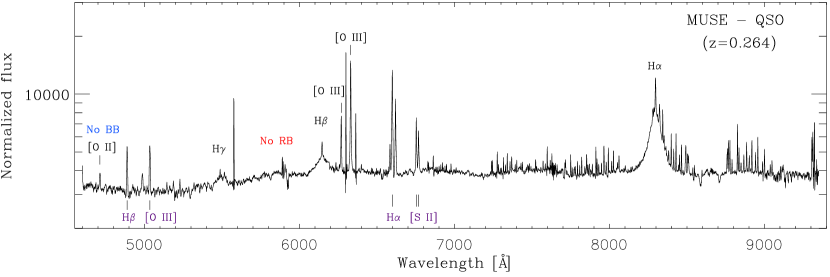
Figure 20: MUSE spectrum of a spurious WR candidate in the Antennae. The false BB and RB, among the strong emission lines identified at z$\sim$0.264, are indicated above the continuum. The BB turned out to be [O ii] $\lambda 3727$. Below the continuum some other lines corresponding to the Antennae (z$\sim$0.005) were identified. The spectrum contains information from astronomical objects at different distances. Its location is indicated in Fig. 1, with a white circle labeled as qso. Flux is normalized to 10^-20 erg cm^-2 s^-1 Å^-1.

Appendix C Nebular emission lines

The spectra of the SSCs with WR features studied here can be used to characterise the physical properties of their environments. The reddening-corrected nebular lines are listed in Table 5. These were used to estimate physical parameters such as $T_{\mathrm{e}}$, $n_{\mathrm{e}}$ and oxygen abundances of the 38 WR spectra reported in Table 3.

Table 5: Reddening-corrected line fluxes, relative to H$\beta$=100.

ID	[O iii]	[O iii]	[S ii]	[S ii]	[N ii]	[N ii]	[N ii]	[Cl iii]	[Cl iii]	[S iii]	[S iii]	[O ii]	[O ii]
	$\lambda 4959$	$\lambda 5007$	$\lambda 6717$	$\lambda 6731$	$\lambda 5755$	$\lambda 6548$	$\lambda 6584$	$\lambda 5517$	$\lambda 5537$	$\lambda 6312$	$\lambda 9069$	$\lambda 7320$	$\lambda 7330$
(1)	(2)	(3)	(4)	(5)	(6)	(7)	(8)	(9)	(10)	(11)	(12)	(13)	(14)
1	59.0$\pm$0.1	176.4$\pm$0.1	28.3$\pm$0.1	24.4$\pm$0.1	0.7$\pm$0.1	31.7$\pm$0.1	95.6$\pm$0.1	0.4$\pm$0.1	0.3$\pm$0.1	1.4$\pm$0.1	46.8$\pm$0.3	3.2$\pm$0.1	2.6$\pm$0.1
2	60.1$\pm$0.1	179.0$\pm$0.1	30.0$\pm$0.1	25.0$\pm$0.1	0.7$\pm$0.1	25.4$\pm$0.1	76.8$\pm$0.1	0.4$\pm$0.1	0.3$\pm$0.1	1.1$\pm$0.1	29.3$\pm$0.2	2.7$\pm$0.1	2.2$\pm$0.1
3	60.6$\pm$0.1	180.2$\pm$0.1	15.8$\pm$0.1	11.9$\pm$0.1	0.5$\pm$0.1	17.7$\pm$0.1	53.1$\pm$0.1	0.4$\pm$0.1	0.3$\pm$0.1	1.0$\pm$0.1	24.1$\pm$0.1	1.6$\pm$0.1	1.3$\pm$0.1
4	34.6$\pm$0.1	101.7$\pm$0.2	35.4$\pm$0.1	26.5$\pm$0.1	0.7$\pm$0.1	26.9$\pm$0.1	81.3$\pm$0.3	0.2$\pm$0.1	0.2$\pm$0.1	0.8$\pm$0.1	17.0$\pm$0.3	1.3$\pm$0.1	1.2$\pm$0.1
5	48.8$\pm$0.1	144.6$\pm$0.1	28.2$\pm$0.1	20.7$\pm$0.1	0.6$\pm$0.1	22.7$\pm$0.1	67.8$\pm$0.1	0.3$\pm$0.1	0.2$\pm$0.1	0.9$\pm$0.1	20.4$\pm$0.2	1.9$\pm$0.1	1.6$\pm$0.1
6	47.7$\pm$0.1	142.0$\pm$0.1	21.0$\pm$0.1	15.3$\pm$0.1	0.6$\pm$0.1	21.7$\pm$0.1	65.5$\pm$0.1	0.3$\pm$0.1	0.2$\pm$0.1	0.9$\pm$0.1	22.1$\pm$0.2	1.5$\pm$0.1	1.3$\pm$0.1
7	3.5$\pm$0.2	10.0$\pm$0.1	28.2$\pm$0.1	22.6$\pm$0.1	0.5$\pm$0.2	34.1$\pm$0.1	104.2$\pm$0.5	$\cdots$	$\cdots$	$\cdots$	8.8$\pm$0.2	0.4$\pm$0.1	0.3$\pm$0.1
8	12.4$\pm$0.1	36.6$\pm$0.1	26.9$\pm$0.1	19.8$\pm$0.1	0.5$\pm$0.1	32.7$\pm$0.1	100.6$\pm$0.4	0.3$\pm$0.1	0.2$\pm$0.1	0.4$\pm$0.1	19.6$\pm$0.1	1.0$\pm$0.1	0.9$\pm$0.1
9	7.9$\pm$0.3	22.8$\pm$0.2	39.1$\pm$0.4	37.6$\pm$0.3	1.1$\pm$0.2	42.9$\pm$0.5	131.4$\pm$1.8	0.3$\pm$0.2	$\cdots$	$\cdots$	13.6$\pm$0.3	1.7$\pm$0.2	1.5$\pm$0.2
10	15.6$\pm$0.2	45.3$\pm$0.1	30.7$\pm$0.1	22.9$\pm$0.1	0.5$\pm$0.1	33.1$\pm$0.2	101.5$\pm$0.7	0.4$\pm$0.2	0.2$\pm$0.1	0.3$\pm$0.1	19.9$\pm$0.1	1.1$\pm$0.1	1.0$\pm$0.1
11	20.0$\pm$0.1	59.0$\pm$0.1	33.1$\pm$0.1	24.5$\pm$0.1	0.6$\pm$0.1	29.1$\pm$0.1	88.6$\pm$0.2	0.2$\pm$0.1	0.2$\pm$0.1	0.4$\pm$0.1	15.0$\pm$0.2	1.3$\pm$0.1	1.2$\pm$0.1
12	17.7$\pm$0.1	52.5$\pm$0.1	31.9$\pm$0.1	23.4$\pm$0.1	0.6$\pm$0.1	30.5$\pm$0.1	92.8$\pm$0.2	0.2$\pm$0.1	$\cdots$	0.4$\pm$0.1	13.9$\pm$0.2	1.2$\pm$0.1	1.3$\pm$0.1
13	24.6$\pm$0.1	72.5$\pm$0.1	19.8$\pm$0.1	14.7$\pm$0.1	0.6$\pm$0.1	29.1$\pm$0.1	88.8$\pm$0.1	0.4$\pm$0.1	0.3$\pm$0.1	0.7$\pm$0.1	22.1$\pm$0.1	1.4$\pm$0.1	1.3$\pm$0.1
14	16.9$\pm$0.1	50.2$\pm$0.1	31.5$\pm$0.1	22.9$\pm$0.1	0.6$\pm$0.1	32.1$\pm$0.1	97.3$\pm$0.2	0.3$\pm$0.1	0.2$\pm$0.1	0.5$\pm$0.1	14.6$\pm$0.2	1.3$\pm$0.1	1.3$\pm$0.1
15	21.2$\pm$0.1	62.8$\pm$0.1	37.1$\pm$0.1	26.2$\pm$0.1	0.7$\pm$0.1	30.7$\pm$0.1	92.7$\pm$0.4	0.3$\pm$0.1	0.3$\pm$0.1	0.4$\pm$0.1	12.6$\pm$0.2	1.5$\pm$0.1	1.7$\pm$0.1
16	14.0$\pm$0.2	40.4$\pm$0.1	27.2$\pm$0.1	19.2$\pm$0.1	0.5$\pm$0.2	29.6$\pm$0.1	89.3$\pm$0.6	0.4$\pm$0.2	1.6$\pm$0.1	0.2$\pm$0.1	13.8$\pm$0.3	0.9$\pm$0.2	1.4$\pm$0.2
17	36.0$\pm$0.1	107.0$\pm$0.2	27.4$\pm$0.1	20.8$\pm$0.1	0.7$\pm$0.1	27.7$\pm$0.1	84.0$\pm$0.4	0.4$\pm$0.1	0.2$\pm$0.1	0.7$\pm$0.1	22.3$\pm$0.1	1.9$\pm$0.1	1.7$\pm$0.1
18	5.8$\pm$0.1	17.1$\pm$0.1	29.3$\pm$0.1	22.0$\pm$0.1	0.6$\pm$0.1	37.1$\pm$0.1	113.4$\pm$0.6	0.2$\pm$0.1	$\cdots$	0.2$\pm$0.1	11.4$\pm$0.3	0.8$\pm$0.1	0.9$\pm$0.1
19	33.9$\pm$0.1	99.2$\pm$0.4	25.5$\pm$0.1	18.1$\pm$0.1	0.7$\pm$0.2	21.6$\pm$0.1	65.3$\pm$0.5	0.4$\pm$0.2	$\cdots$	0.3$\pm$0.2	15.5$\pm$0.2	1.1$\pm$0.2	1.4$\pm$0.1
20	46.5$\pm$0.1	137.9$\pm$0.4	34.0$\pm$0.1	24.1$\pm$0.1	0.5$\pm$0.1	21.4$\pm$0.1	64.7$\pm$0.3	0.3$\pm$0.1	0.2$\pm$0.1	0.6$\pm$0.1	16.1$\pm$0.2	1.9$\pm$0.1	2.3$\pm$0.2
21	41.4$\pm$0.1	122.0$\pm$0.2	28.4$\pm$0.1	21.2$\pm$0.1	0.7$\pm$0.1	25.8$\pm$0.1	80.0$\pm$0.2	0.4$\pm$0.1	0.3$\pm$0.1	0.8$\pm$0.1	21.1$\pm$0.2	2.6$\pm$0.1	2.6$\pm$0.1
22	13.3$\pm$0.1	39.5$\pm$0.1	34.0$\pm$0.2	25.7$\pm$0.1	0.6$\pm$0.1	35.0$\pm$0.2	107.0$\pm$0.7	0.3$\pm$0.1	$\cdots$	0.3$\pm$0.1	14.5$\pm$0.3	1.0$\pm$0.1	1.0$\pm$0.1
23	9.7$\pm$0.2	28.2$\pm$0.1	41.2$\pm$0.2	30.3$\pm$0.2	0.6$\pm$0.2	33.8$\pm$0.2	103.1$\pm$0.7	0.3$\pm$0.1	$\cdots$	0.2$\pm$0.1	10.3$\pm$0.2	0.8$\pm$0.1	0.6$\pm$0.1
24	7.4$\pm$0.1	21.9$\pm$0.1	29.9$\pm$0.1	22.6$\pm$0.1	0.5$\pm$0.1	34.7$\pm$0.1	105.9$\pm$0.3	0.3$\pm$0.1	$\cdots$	0.3$\pm$0.1	14.8$\pm$0.1	0.7$\pm$0.1	0.5$\pm$0.1
25	6.9$\pm$0.1	20.2$\pm$0.1	32.9$\pm$0.1	24.2$\pm$0.1	0.6$\pm$0.1	32.1$\pm$0.1	97.6$\pm$0.4	0.3$\pm$0.1	$\cdots$	0.2$\pm$0.1	11.5$\pm$0.1	0.6$\pm$0.1	0.4$\pm$0.1
26	15.3$\pm$0.2	44.0$\pm$0.1	39.4$\pm$0.2	29.6$\pm$0.1	0.8$\pm$0.2	30.9$\pm$0.1	94.5$\pm$0.8	0.7$\pm$0.3	$\cdots$	0.3$\pm$0.1	11.9$\pm$0.3	0.9$\pm$0.2	0.7$\pm$0.2
27	8.7$\pm$0.2	25.4$\pm$0.1	38.2$\pm$0.1	27.5$\pm$0.1	0.5$\pm$0.1	30.8$\pm$0.1	93.9$\pm$0.5	0.3$\pm$0.1	$\cdots$	0.1$\pm$0.1	10.0$\pm$0.2	0.6$\pm$0.1	0.2$\pm$0.1
28	8.3$\pm$0.2	23.7$\pm$0.1	40.7$\pm$0.2	30.0$\pm$0.1	0.6$\pm$0.2	32.8$\pm$0.1	100.3$\pm$0.7	0.4$\pm$0.2	0.2$\pm$0.1	0.2$\pm$0.1	9.5$\pm$0.2	0.7$\pm$0.1	0.5$\pm$0.1
29	14.7$\pm$0.1	42.8$\pm$0.1	37.8$\pm$0.1	27.2$\pm$0.1	0.7$\pm$0.2	29.9$\pm$0.1	90.7$\pm$0.4	0.4$\pm$0.1	$\cdots$	0.3$\pm$0.1	12.2$\pm$0.2	0.9$\pm$0.1	0.7$\pm$0.1
30	13.3$\pm$0.1	39.3$\pm$0.1	40.3$\pm$0.1	29.5$\pm$0.1	0.7$\pm$0.1	34.0$\pm$0.1	103.8$\pm$0.3	0.3$\pm$0.1	0.2$\pm$0.1	0.4$\pm$0.1	14.5$\pm$0.1	1.1$\pm$0.1	0.9$\pm$0.1
31	9.7$\pm$0.1	28.8$\pm$0.1	29.2$\pm$0.1	25.2$\pm$0.1	0.7$\pm$0.1	45.6$\pm$0.1	139.7$\pm$0.1	0.2$\pm$0.1	0.2$\pm$0.1	0.4$\pm$0.1	21.6$\pm$0.1	1.4$\pm$0.1	1.1$\pm$0.1
32	4.5$\pm$0.2	12.9$\pm$0.1	31.7$\pm$0.1	23.5$\pm$0.1	0.7$\pm$0.2	34.1$\pm$0.1	104.0$\pm$0.1	0.3$\pm$0.2	$\cdots$	0.1$\pm$0.1	10.0$\pm$0.2	0.5$\pm$0.1	0.3$\pm$0.1
33	3.8$\pm$0.1	11.3$\pm$0.1	31.3$\pm$0.2	23.9$\pm$0.1	0.4$\pm$0.1	34.5$\pm$0.1	105.6$\pm$0.5	0.3$\pm$0.2	$\cdots$	0.1$\pm$0.1	10.0$\pm$0.1	0.5$\pm$0.1	0.3$\pm$0.1
34	11.3$\pm$0.1	32.7$\pm$0.1	37.0$\pm$0.2	26.7$\pm$0.1	0.7$\pm$0.2	34.6$\pm$0.2	105.7$\pm$0.8	0.3$\pm$0.2	1.4$\pm$0.1	0.2$\pm$0.1	12.4$\pm$0.2	0.9$\pm$0.1	0.7$\pm$0.1
35	2.6$\pm$0.3	5.6$\pm$0.2	26.1$\pm$0.1	19.4$\pm$0.1	0.5$\pm$0.2	26.6$\pm$0.2	81.8$\pm$1.0	0.4$\pm$0.3	$\cdots$	$\cdots$	5.6$\pm$0.2	0.3$\pm$0.2	0.2$\pm$0.2
36	21.9$\pm$0.3	62.8$\pm$0.2	44.2$\pm$0.5	32.1$\pm$0.3	1.0$\pm$0.4	28.2$\pm$0.1	86.0$\pm$0.9	0.6$\pm$0.3	0.5$\pm$0.3	0.3$\pm$0.2	11.2$\pm$0.4	0.9$\pm$0.3	0.5$\pm$0.3
37	13.2$\pm$0.2	38.9$\pm$0.1	45.6$\pm$0.2	32.3$\pm$0.1	0.7$\pm$0.1	29.0$\pm$0.1	88.7$\pm$0.5	0.3$\pm$0.1	$\cdots$	$\cdots$	10.0$\pm$0.2	1.1$\pm$0.1	0.9$\pm$0.1
38	24.2$\pm$0.1	71.2$\pm$0.2	42.1$\pm$0.5	29.9$\pm$0.3	0.7$\pm$0.2	28.5$\pm$0.2	87.4$\pm$1.0	0.4$\pm$0.2	0.2$\pm$0.2	0.5$\pm$0.1	15.0$\pm$0.1	1.4$\pm$0.2	1.2$\pm$0.2

References

- Asplund et al. (2009) Asplund, M. et al. 2009, ARA&A, 47, 481-522
- Bacon et al. (2010) Bacon, R. et al. 2010, Proc. SPIE, 7735, 773508
- Bastian et al. (2006) Bastian, N. et al. 2006, A&A, 445, 471-483
- Bastian et al. (2009) Bastian, N. et al. 2009, ApJ, 701, 607-619
- Berg et al. (2015) Berg, D. A. et al. 2015, ApJ, 806, 16
- Brinchmann et al. (2008) Brinchmann, J., Kunth, D., & Durret, F. 2008, A&A, 485, 657
- Cabrera-Lavers (2016) Cabrera-Lavers, A. 2016, ASP Conf. Ser., 507, 185
- Cardelli et al. (1989) Cardelli, J. A. A. et al. 1989, ApJ, 345, 245
- Crowther & Hadfield (2006) Crowther, P. A., & Hadfield, L. J. 2006, A&A, 449, 711
- Crowther (2007) Crowther, P. A. 2007, ARA&A, 45, 177
- Crowther (2019) Crowther, P. A. 2019, Galaxies, 7, 88
- Chávez et al. (2016) Chávez, R. et al. 2016, MNRAS, 462, 2431-2439
- Eldridge et al. (2017) Eldridge, J. J. et al. 2017, Publ. Astron. Soc. Australia, 34, e058
- Garnett (1992) Garnett, D. R. 1992, AJ, 103, 1330
- Gómez-González et al. (2016) Gómez-González, V. M. A. et al. 2016, MNRAS, 460, 1555
- Gómez-González et al. (2020) Gómez-González, V. M. A. et al. 2020, MNRAS, 493, 3879-3892
- Gunawardhana et al. (2019) Gunawardhana, M. L. P. et al. 2019, arXiv:1912.08151
- Hadfield & Crowther (2007) Hadfield, L. J., & Crowther, P. A. 2007, MNRAS, 381, 418
- Hadfield & Crowther (2006) Hadfield, L. J., & Crowther, P. A. 2006, MNRAS, 368, 1822-1832
- James et al. (2020) James, B. L. et al. 2020, MNRAS, 495, 2564-2581
- Kehrig et al. (2011) Kehrig, C. et al. 2011, A&A, 526, A128
- Kehrig et al. (2018) Kehrig, C. et al. 2018, MNRAS, 480, 1081-1095
- Kehrig et al. (2013) Kehrig, C. et al. 2013, MNRAS, 432, 2731-2745
- Knapen et al. (2015) Knapen, J. H. et al. 2015, MNRAS, 454, 1742-1750
- Kunth & Östlin (2000) Kunth,D. & Östlin, G. 2000, A&ARv, 10, 1-79
- Lada & Lada (2003) Lada, C. J., & Lada, E. A. 2003, ARA&A, 41, 57-115
- Lardo et al. (2015) Lardo, C. et al. 2015, ApJ, 812, 160
- Li et al. (2008) Li, Ch. et al. 2008, MNRAS, 385, 1903-1914
- López-Sánchez & Esteban (2010) López-Sánchez, Á. R., & Esteban, C. 2010, A&A, 516, A104
- Luridiana et al. (2015) Luridiana, V., Morisset, C. & Shaw R. A. 2015, A&A, 573, A42
- Maeder (1992) Maeder, A. 1992, A&A, 264, 105-120
- Matthews et al. (2018) Matthews, A. M. et al. 2018, ApJ, 862, 147
- Mayya et al. (2020) Mayya, Y. D. et al. 2020, arXiv:2008.00320
- Metz et al. (2004) Metz, J. M. et al. ApJ, 605, 725-741
- Miralles-Caballero et al. (2014) Miralles-Caballero, D. et al. 2014, MNRAS, 440, 2265
- Monreal-Ibero et al. (2017) Monreal-Ibero, A. et al. 2017, A&A, 603, A130
- Moffat (2015) Moffat, A. F. J. 2015, 2015wrs..conf, 13M
- Neugent et al. (2012) Neugent, K. F., Massey, P., Georgy, C. 2012, ApJ, 759, 11
- Neugent & Massey (2019) Neugent, K., Massey, P. 2019, Galaxies, 7, 74
- Ott (2012) Ott, T., QFitsView: FITS file viewer, ascl:1210.019
- Osterbrock & Ferland (2006) Osterbrock, D. E., & Ferland, G. J. 2006, Astrophysics of gaseous nebulae and active galactic nuclei
- Portegies-Zwart et al. (2010) Portegies Zwart, S. F. et al. ARA&A, 48, 431-493
- Press et al. (1992) Press, W. H. et al. 1992, Cambridge: University Press
- Riess et al. (2016) Riess, A. G. et al. 2016, ApJ, 826, 56
- Rosslowe & Crowther (2015) Rosslowe, C. K., & Crowther, P. A 2015, MNRAS, 447, 2322-2347
- Schaerer & Vacca (1998) Schaerer, D., & Vacca, W. D. 1998, ApJ, 497, 618-644
- Schaerer et al. (2019) Schaerer, D., Fragos, T., Izotov, Y. I. 2019, A&A, 622, L10
- Schweizer et al. (2008) Schweizer, F. et al. 2008, AJ, 136, 1482
- Schlafly & Finkbeiner (2011) Schlafly, E. F., & Esteban, D. P. 2011, ApJ, 737, 103
- Smith et al. (2007) Smith, B. J. et al. 2007, AJ, 133, 791-817
- Tody (1993) Tody, D. 1993, Astronomical Data Analysis Software and Systems II, 173
- Tramper (2015) Tramper, F. et al. 2015, A&A, 581, A110
- Tresse et al. (1999) Tresse et al. 1999, MNRAS, 310, 262
- Vacca & Conti (1992) Vacca, W. D. & Conti, P. S. 1992, ApJ, 401, 543
- Vanbeveren (2007) Vanbeveren, D. et al. 2007, ApJ, 662, L107-L110
- Weilbacher et al. (2018) Weilbacher, P. M. et al. 2018, A&A, 611, A95
- Whitmore & Schweizer (1994) Whitmore, B. C., & Schweizer, F. 1994, AAS, 26, 1488
- Whitmore et al. (2005) Whitmore, B. C. et al. 2005, AJ, 130, 2104-2116
- Whitmore (2009) Whitmore, B. C. 2009, msfp.book, 104-115
- Whitmore et al. (2010) Whitmore, B. C. et al. 2010, AJ, 140, 75-109
- Woosley & Bloom (2006) Woosley, S. E. & Bloom, J. S. 2006, ARA&A, 44, 507-556
- Woosley & Heger (2006) Woosley, S. E. & Heger, A. 2006, ApJ, 637 914-921
- Zhang et al. (2001) Zhang, Q. et al. 2001, ApJ, 561, 727-750