Enhancing searches for resonances with machine learning and moment decomposition

Abstract

A key challenge in searches for resonant new physics is that classifiers trained to enhance potential signals must not induce localized structures. Such structures could result in a false signal when the background is estimated from data using sideband methods. A variety of techniques have been developed to construct classifiers which are independent from the resonant feature (often a mass). Such strategies are sufficient to avoid localized structures, but are not necessary. We develop a new set of tools using a novel moment loss function (Moment Decomposition or MoDe) which relax the assumption of independence without creating structures in the background. By allowing classifiers to be more flexible, we enhance the sensitivity to new physics without compromising the fidelity of the background estimation.

1 Introduction

Searching for new phenomena associated with localized excesses in otherwise featureless spectra, often referred to as bump hunting, is one of the most widely used approaches in particle and nuclear physics, dating back at least to the discovery of the $\rho$ meson Button:1962bnf , and used continuously since, including recently in the discovery of the Higgs boson Aad:2012tfa ; Chatrchyan:2012ufa . In the present day, such searches reach the multi-TeV scale Sirunyan:2019vgj ; Aad:2019hjw and span high energy particle and nuclear physics experiments Aaij:2020ikh ; Adam:2020zsu ; Acharya:2020jil ; Adrian:2018scb ; McCracken:2015coa ; Ablikim:2019rpl ; BelleII:2020fag . A key feature of these searches is that they are relatively background model agnostic since sidebands in data can be used to estimate the background under a potential localized excess. These sideband fits are possible because the background data can be well-approximated either with simple parametric functions or smooth non-parametric techniques such as Gaussian processes Frate:2017mai .

Sideband methods for background estimation are often combined with relatively simple and robust event selections in order to ensure broad coverage of new physics model space. However, there is a growing use of modern machine learning techniques to enhance signal sensitivity Larkoski:2017jix ; Guest:2018yhq ; Albertsson:2018maf ; Radovic:2018dip ; Bourilkov:2019yoi . For example, both ATLAS Aaboud:2018psm and CMS Sirunyan:2020lcu have developed machine-learning-based $W$ jet taggers that improve the sensitivity of searches involving Lorentz-boosted and hadronically decaying $W$ bosons. Boosted electroweak bosons are common in searches for models with a significant mass hierarchy between the primary resonance mass and the $W$ boson mass Aad:2019fbh ; Aad:2020ddw ; Sirunyan:2019jbg ; Sirunyan:2019vgt ; Aad:2020tps ; Sirunyan:2018fuh ; Aad:2020ldt ; Sirunyan:2019quj ; Sirunyan:2017isc ; Aad:2020hzm ; Aaboud:2017ecz ; Aad:2020cws , and boosted $W$-like particles are a feature of searches for low-mass dark matter mediators Aaboud:2018zba ; Sirunyan:2017dnz ; Sirunyan:2018ikr ; Sirunyan:2019sgo ; Sirunyan:2019vxa ; ATLAS-CONF-2018-052 ; Sirunyan:2017dgc .

A key challenge with complex event selections like those involved in boosted $W$ tagging is that they can invalidate the smoothness assumption of the background. In particular, if classifiers can infer the mass of the parent resonance, then selecting signal-like events will simply pick out background events with a reconstructed mass near the target resonance mass. Many techniques have been developed that modify or simultaneously optimize classifiers so that their responses are independent of a given resonance feature NIPS2017_6699 ; Dolen:2016kst ; Moult:2017okx ; Stevens:2013dya ; Shimmin:2017mfk ; Bradshaw:2019ipy ; ATL-PHYS-PUB-2018-014 ; DiscoFever ; Xia:2018kgd ; Englert:2018cfo ; Wunsch:2019qbo ; Rogozhnikov:2014zea ; 10.1088/2632-2153/ab9023 ; clavijo2020adversarial ; Kasieczka:2020pil ; Chang:2017kvc ; Clavijo:2020mua ; Sirunyan:2019nfw ; Stevens:2013dya ; Rogozhnikov:2014zea . For machine learning classifiers, the proposed solutions include modifications to loss functions that implicitly or explicitly enforce independence. These methods have been successfully deployed in bump hunts; see, e.g., Refs. Sirunyan:2017dnz ; Sirunyan:2017dgc ; Sirunyan:2017nvi ; Aaboud:2018zba ; Sirunyan:2018ikr ; Sirunyan:2018gdw ; Sirunyan:2018sgc ; Sirunyan:2019sgo ; Sirunyan:2019jbg ; Sirunyan:2019vxa ; Aad:2020cws ; Sirunyan:2020hwz ; Aaij:2020ypa ; Aaij:2020hon ; Aaij:2019mhf ; Aaij:2018xpt ; Aaij:2015tna ; Aaij:2017eru ; Aaij:2016vsy . A variety of similar proposals under the monikers of domain adaptation and fairness have been proposed in the machine learning literature (see e.g. Ref. DBLP:journals/corr/EdwardsS15 ; JMLR:v17:15-239 and Ref. mehrabi2019survey ; alex2018frontiers ).

Ensuring that a classifier is independent from a given resonant feature is sufficient for mitigating sculpting, but it is not necessary. The original requirement is simply that a selection using the classifier does not introduce localized features in the background spectrum, which is a much looser requirement than enforcing independence. For example, if a classifier has a linear dependence on the resonant feature, then there would be a strong correlation. However, a threshold requirement on such a classifier would not sculpt any bumps in the background-only case. This example motivates a new class of techniques that allow classifiers to depend on the resonant feature in a controlled way. In the limit that constant dependence is required, then the classifier and the resonant feature will be independent. The advantage of relaxing the independence requirement is that the resulting classifiers can achieve superior performance because they are allowed to be more flexible.

In this article, we present a new set of tools that allow for controlled dependence on a resonant feature. This new approach is called Moment Decomposition (MoDe). Using MoDe, analysts can require independence, linear dependence, and quadratic dependence. In addition, analysts can place bounds on the slope of the linear dependence, and restrict quadratic dependence to be monotonic. Extending MoDe to allow for arbitrarily higher-order dependence is straightforward. This article is organized as follows. Section 2 briefly reviews existing decorrelation methods and then introduces MoDe. Numerical results using a simplified model and a physically motivated example are presented in Sec. 3. Finally, we present conclusions and outlook in Sec. 4.

2 Methods

2.1 Existing decorrelation methods

We will consider the binary classification setting in which examples are given by the triplet $(X,Y,M),$ where $X\in\mathcal{X}$ is a feature vector, $Y\in\mathcal{Y}:=\{0,1\}$ is the target label, and finally, $M\in\mathcal{M}$ is the resonant feature (or protected attribute) whose spectrum will be used in the bump hunting. Throughout this article, we take $M$ to be mass, though it could be any feature. The feature vector $X$ can either contain $M$ directly as one of its elements or contain other features that are arbitrarily indicative of $M$. We are interested in finding a mapping $f:\mathcal{X}\rightarrow\mathcal{S}$ where $s\in\mathcal{S}$ are scores used to obtain predictions $\hat{y}\in\mathcal{Y}$ with the additional constraint that $f$ be conditionally independent of (or uniform with) $M$ in the sense that

$$p(f(X)=s|M=m,Y=y)=p(f(X)=s|Y=y)\;\forall\;m\in\mathcal{M}\;\text{and}\;\forall\;s\in\mathcal{S},$$ (1)

for one or more values $y$, although typically, Eq. (1) is required only for the background.

Existing decorrelation methods used in particle physics that simultaneously train a classifier $f(x):\mathbb{R}^{n}\rightarrow[0,1]$ and decorrelate from a resonant feature $m$ use the following loss function:

$$\mathcal{L}[f(x)]=\sum_{i\in\text{S}}L_{\text{class}}(f(x_{i}),1)+\sum_{i\in\text{B}}w(m_{i})\,L_{\text{class}}(f(x_{i}),0)+\lambda\sum_{i\in\text{B}}L_{\text{decor}}(f(x_{i}),m_{i})\,,$$ (2)

where $S=\{i|\,y_{i}=1\}$ and $B=\{i|\,y_{i}=0\}$ denote signal and background, respectively, $L_{\text{class}}$ is the usual classification loss such as the binary cross entropy $L_{\text{BCE}}(f(x),y)=y\log(f(x))+(1-y)\log(1-f(x))$, $w$ is a weighting function, $\lambda$ is a hyperparameter, and $L_{\text{decor}}$ generically denotes some form of decorrelation loss. Standard classification corresponds to $w(m)=1$ and $\lambda=0$. Decorrelation methods include:

• Planing Chang:2017kvc ; 1511.05190 : $\lambda=0$ and $w(m_{i})\approx p_{S}(m)/p_{B}(m)$ so that the marginal distribution of $m$ is non-discriminatory after the reweighting.

• Adversaries NIPS2017_6699 ; Shimmin:2017mfk ; Englert:2018cfo ; Clavijo:2020mua : $w(m)=1$, $\lambda<0$, and $L_{\text{decor}}$ is the loss of a second neural network (adversary) that takes $f(x)$ as input and tries to learn some properties of $m$ or its probability density.

• Distance Correlation (DisCo) DiscoFever ; Kasieczka:2020pil : $w(m)=1,\lambda>0$, and the last term in Eq. (2) is the distance correlation szekely2007 ; szekely2009 ; SzeKely:2013:DCT:2486206.2486394 ; szekely2014 between $f(x)$ and $m$ for the background.

• Flatness Rogozhnikov:2014zea : $w(m)=1$, $\lambda>0$, and $L_{\text{decor}}=\sum_{m}b_{m}\int|F_{m}(s)-F(s)|^{2}\,{\rm d}s$ where the sum runs over mass bins, $b_{m}$ is the fraction of candidates in bin $m$, $F$ is the cumulative distribution function, and $s=f(x)$ is the classifier output.

Decorrelation methods have proven to be useful additions to the toolkit of the bump hunter.

2.2 Moment decorrelation

First, we will derive a new decorrelation method based on moments. While this technique achieves state-of-the-art decorrelation performance, along with being robust, simple, and fast, its true value is that it is trivially extended to allow for controlled dependence beyond just decorrelation.

We begin by noting that the uniformity constraint in Eq. (1) can be written in terms of the conditional cumulative distribution function (CDF) of scores at $s$, $F(s|M,Y)$, as

$$F(f(X)=s|Y=y)=F(f(X)=s|M=m,Y=y)\;\forall\;m\in\mathcal{M}\;\text{and}\;\forall\;s\in\mathcal{S}.$$ (3)

This is the same observation that lies at the heart of the flatness loss defined in Ref. Rogozhnikov:2014zea . Here, we will consider the conditional CDFs in bins of mass and only on the background, which allows us to adopt the following more compact notation

$$F(f(X)=s|M=m,Y=y)\to F_{m}(s),$$ (4)

where now $m$ is discrete and indexes the mass bins. We leave the exploration of similar unbinned approaches for future work. Furthemore, we assume that some transformation is performed on $m$ such that $\mathcal{M}\to[-1,1]$. This could be a simple linear transformation but does not have to be, discussion on this point is provided later.

The uniformity constraint of Eq. (3) can be imposed on the learned function by defining the decorrelation loss using

$$L_{\rm decor}\to L_{\rm\sc MoDe}^{0}\equiv\sum_{m}\int|F_{m}(s)-F_{m}^{0}(s)|^{2}{\rm d}s.$$ (5)

Here, $F^{0}_{m}$ is based on the 0^th Legendre moment of $F_{m}(s)$ in $m$, $c_{0}$, and polynomial, $P_{0}(x)=1$, as

$$F^{0}_{m}(s)=c_{0}(s)P_{0}(\tilde{m})=\frac{1}{2}\int_{-1}^{+1}P_{0}(m^{\prime})F(s|m^{\prime}){\rm d}m^{\prime}\approx\frac{1}{2}\sum_{m^{\prime}}\Delta_{m^{\prime}}F_{m^{\prime}}(s),$$ (6)

where $\Delta_{m}$ denotes the width of bin $m$, and $\tilde{m}$ is its central mass value. Note that the loss in Eq. (5) is clearly minimized when

$$F_{m}(s)=F_{m}^{0}(s)=c_{0}(s)\;\forall\;m,$$ (7)

which implies that Eq. (3) holds and $f(X)$ and $M$ are indeed independent. Note that in the limit that all bins have equal width and occupancy, it is straightforward to show that the loss function in Eq. (5) is the same as the flatness loss of Ref. Rogozhnikov:2014zea ; however, when the underlying background distribution is highly nonuniform, these loss functions are drastically different resulting in MoDe outperforming Ref. Rogozhnikov:2014zea in such cases.

2.3 Beyond decorrelation: Moment decomposition

We will now generalize moment decorrelation to allow for controllable mass dependence in the form of an $\ell^{\rm th}$ order polynomial, where $\ell$ is a hyperparameter chosen by the analyst. The generalized MoDe loss is given by

$$\mathcal{L}[f]=L_{\mathrm{class}}+\lambda L^{\ell}_{\mathrm{\textsc{MoDe}},}$$ (8)

where

$$L_{\rm\sc MoDe}^{\ell}\equiv\sum_{m}\int|F_{m}(s)-F_{m}^{\ell}(s)|^{2}{\rm d}s.$$ (9)

Here, $F^{0}_{m}$ in Eq. (5) has been replaced by

$$F_{m}^{\ell}(s)=\sum_{l=0}^{\ell}c_{l}(s)P_{l}(\tilde{m}),$$ (10)

and the Legendre moments are given by

$$c_{l}(s)=\left[\frac{2l+1}{2}\right]\int_{-1}^{1}P_{l}(m^{\prime})F(s|m^{\prime}){\rm d}m^{\prime}\approx\left[\frac{2l+1}{2}\right]\sum_{m^{\prime}}\Delta_{m^{\prime}}P_{l}(\tilde{m}^{\prime})F_{m^{\prime}}(s).$$ (11)

We note that setting $\ell=0$ reduces the generalized MoDe loss of Eq. (9) down to the moment decorrelation of Eq. (5).

The MoDe loss in Eq. (9) is optimal when $F_{m}(s)=F^{\ell}_{m}(s)\;\forall\;m,s$, which clearly occurs when the mass dependence of the classifier is at most an $\ell^{\rm th}$ order polynomial. For example, taking $\ell=0$ drives the classifier to be independent of mass. More interestingly, choosing $\ell=1$ allows for a linear mass dependence, $\ell=2$ quadratic dependence, etc. Furthermore, making the replacement

$$c_{1}(s)\to c_{1}^{\rm max}c_{0}(s)\tanh{\left(\frac{c_{1}(s)}{c_{1}^{\rm max}c_{0}(s)}\right)}$$ (12)

in Eq. (10) places an upper limit $c_{1}^{\rm max}c_{0}(s)>0$ on the magnitude of the linear slope (the first Legendre moment is the coefficient of the $\tilde{m}$ term), allowing the analyst to control this aspect of the mass dependence through a hyperparameter, $c_{1}^{\rm max}$. In addition, for the case where $\ell=2$ is selected, it is straightforward to show that as long as ${3|c_{2}(s)|\leq|c_{1}(s)|}$ the derivative of $F^{\ell}_{m}(s)$ is nonzero on $(-1,1)$. Therefore, making the replacement

$$c_{2}(s)\to\frac{c_{1}(s)}{3}\tanh{\left(\frac{3c_{2}(s)}{c_{1}(s)}\right)}$$ (13)

in Eq. (10) results in monotonic mass dependence. This option can be turned on or off in MoDe, and can be used in conjunction with $c_{1}^{\rm max}$ if desired. Finally, controlled higher-order mass dependence can be achieved by extending these ideas to larger $\ell$ values.

2.4 Computational details

Computing the MoDe loss and its gradient is straightforward using a few approximations. At the batch level,

$$F_{m}(s)\approx\frac{1}{n_{m}}\sum_{i=1}^{n}\Theta(s-s_{i})\delta_{m,m_{i}},$$ (14)

where $n$ is the number of samples in the batch, $n_{m}$ is the number of samples in bin $m$, $s_{i}\equiv f(x_{i})$ is the score of sample $i$, and $\Theta$ is the Heaviside function: $\Theta(x)=1$ if $x>0$ and $\Theta(x)=0$ otherwise. Minimizing the loss function requires calculating the functional derivative of $L_{\sc\rm MoDe}^{\ell}$ with respect to $f$. This requires specifying how the MoDe loss changes due to variations of the score of each sample in the batch:

$$\delta L_{\sc\rm MoDe}^{\ell}=\delta s_{i}\sum_{m}\int 2\left[F_{m}(s)-F^{\ell}_{m}(s)\right]\left[\frac{\partial F_{m}}{\partial s_{i}}-\frac{\partial F^{\ell}_{m}}{\partial s_{i}}\right]{\rm d}s,$$ (15)

where from Eq. (14)

$$\frac{\partial F_{m}}{\partial s_{i}}\approx-\frac{1}{n_{m_{i}}}\delta(s-s_{i})\delta_{m,m_{i}}.$$ (16)

In addition, using this result, along with Eqs. (10) and (11), we obtain

$$\frac{\partial F^{0}_{m}}{\partial s_{i}} \approx\frac{1}{2}\Delta_{m_{i}}\frac{\partial F_{m_{i}}}{\partial s_{i}}=-\frac{\Delta_{m_{i}}}{2n_{m_{i}}}\delta(s-s_{i}),$$ (17)

$$\frac{\partial F^{1}_{m}}{\partial s_{i}} \approx\frac{\partial F^{0}_{m}}{\partial s_{i}}+\frac{3}{2}\tilde{m}\cdot\tilde{m}_{i}\Delta_{m_{i}}\frac{\partial F_{m_{i}}}{\partial s_{i}}=-\frac{\Delta_{m_{i}}}{2n_{m_{i}}}\delta(s-s_{i})\left[1+3\tilde{m}\cdot\tilde{m}_{i}\right],$$ (18)

$$\vdots$$

where the sum over mass bins in Eq. (11) is no longer needed, since changes to the score for sample $i$ only affect the CDF in bin $m_{i}$. The factors of $\delta(s-s_{i})$ eliminate the integral over $s$ resulting in relatively simple gradient terms, e.g., for $\ell=1$ we obtain

$$\delta L_{\sc\rm MoDe}^{1}\approx-\delta s_{i}\sum_{m}\frac{1}{n_{m_{i}}}\left[F_{m}(s)-F^{1}_{m}(s)\right]\left[2\delta_{m,m_{i}}-\Delta_{m_{i}}(1+3\tilde{m}\cdot\tilde{m}_{i})\right].$$ (19)

The fact that terms like Eq. (19) do not depend on how the integral over $s$ is approximated yields high-precision gradients, which is a big advantage when performing gradient descent.

The results in this subsection are easily generalized for weighted samples. The CDFs in Eq. (14) become

$$F_{m}(s)\approx\frac{1}{w_{m}}\sum_{i}^{n}w_{i}\Theta(s-s_{i})\delta_{m,m_{i}},$$ (20)

where $w_{i}$ are the per-sample weights and

$$w_{m}=\sum_{i}^{n}w_{i}\delta_{m,m_{i}}$$ (21)

is the sum of the weights in bin $m$. Equation (16) then becomes

$$\frac{\partial F_{m}}{\partial s_{i}}\approx-\frac{w_{i}}{w_{m_{i}}}\delta(s-s_{i})\delta_{m,m_{i}},$$ (22)

and updating the rest of the results follows accordingly.

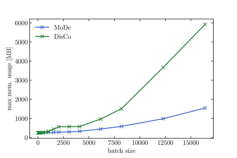
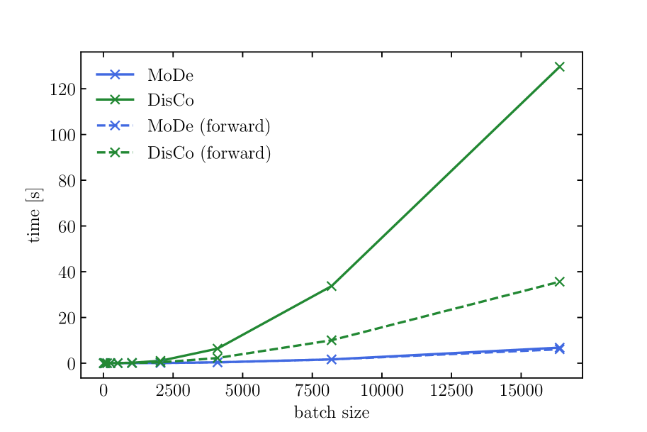
Finally, we address the topic of scalability. While the optimization of the MoDe loss works well stochastically with few examples every step, its performance increases greatly with larger batch sizes. This is not surprising due to the global nature of the MoDe constraint. Fortunately, all of the calculations scale well with batch size (see Appendix A for time and memory performance as functions of the number of inputs). Most computational costs occur in the forward direction, where MoDe scales linearly with the number of inputs $n$ (batch size) and the number of steps chosen for the integral in $s$, $n_{s}$. In addition, dynamic binning sorts $m_{i}$ and reindexes $s_{i}$ are required, and so MoDe runs in $\mathcal{O}(n_{s}\times n+n\log n)$ time. In the forward direction, we also compute and cache the residual $F_{m}(s_{i})-\tilde{F}_{m}(s_{i})$ which is used in the backward pass. Since the CDFs are evaluated at every $s_{i}$, this contributes an $\mathcal{O}(n\times n_{m})$ component. In theory, this could be improved, e.g., if the CDFs at $s_{i}$ were instead approximated using nearest neighbor interpolation. Finally, MoDe takes $\mathcal{O}(n\times n_{m})$ extra memory (beyond what is required to store the data) when calculating the gradients, since the CDF is computed for each input for each bin. It is worth noting that, at particularly small batch sizes, MoDe might be susceptible to slow convergence due to mini-batch statistics not accurately reflecting the full-batch statistics. That is why we recommend using MoDe with a sizeable fraction of the full sample.

3 Example Results

In this section, we will demonstrate how MoDe performs on a simple model problem, and on the $W$-jet tagging problem used in the decorrelation studies of Ref. DiscoFever ; ATL-PHYS-PUB-2018-014 . All of the numerical results reported in this section are obtained using the PyTorch framework NEURIPS2019_9015 .

3.1 Simple Model

We first consider a binary classification example composed of a signal and two types of background. Each sample $X\in\mathcal{X}$ has 2 features:

$$x_{1} \sim\begin{cases}\mathcal{N}\big{(}1,1\big{)}\quad&\quad\text{when}\;Y=1,\\ \mathcal{N}\big{(}0,1\big{)}\quad&\quad\text{when}\;Y=0\;\text{for background type 1},\\ \mathcal{N}\big{(}-4,1\big{)}\quad&\quad\text{when}\;Y=0\;\text{for background type 2},\\ \end{cases}$$ (23)

$$x_{2} =\exp\left[-\frac{(m-0.2)^{2}}{2\cdot 0.1^{2}}\right]\;\;\text{when}\;Y=0\;\text{or }Y=1,$$ (24)

where $\mathcal{N}$ denotes the normal distribution. The mass, $m$, is drawn from $\mathcal{N}(0.2,0.1)$ and $\mathcal{U}(-1,1)$ at equal rates when $Y=1$. For the backgrounds, we sample a uniform random variable, $U\sim\mathcal{U}(0,1)$, then define $m=1-2\sqrt{U}$ and $m=-1+2\sqrt{U}$ for background types 1 and 2, respectively. This simple-model data is shown in Fig. 1.

Figure 1: Simple model distributions.

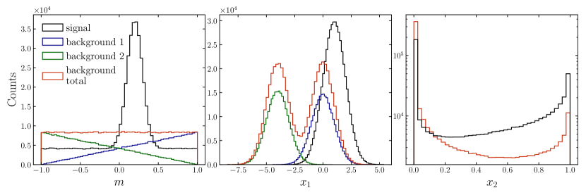
In this scenario, an unconstrained classifier with sufficient capacity will learn the underlying mass distribution (due to the explicit mass dependence of $x_{2}$) and use it to discriminate between signal and background. Figure 2 shows how such a classifier favors regions near $m=0.2$, leading to extreme peak-sculpting in the background. It would be difficult to employ this classifier in a real-world analysis and obtain an unbiased signal estimator. Figure 2 also shows that MoDe[0] successfully decorrelates the classifier response from mass producing a viable classifier for such an analysis.

Figure 2: Left: The false positive rate versus mass for various models at signal efficiencies $\epsilon^{\text{rel}}_{\text{sig}}=80,50,20\%$ (each set of 3 identically colored and stylized lines correspond to the same model but with selection thresholds chosen to achieve the 3 desired signal efficiencies). The bottom panel shows that MoDe[1] and MoDe[2] completely overlap with the $m$-agnostic model for this simple example, which is expected because the optimal classifier here has linear dependence on mass (see text). Right: ROC curves for MoDe[0], MoDe[1], and MoDe[2] compared to the $m$-agnostic model and a model with unconstrained mass dependence. As in the left panel, we see that MoDe[1], MoDe[2], and the $m$-agnostic ROC curves are nearly identical because the optimal classifier has linear mass dependence in this simple example.

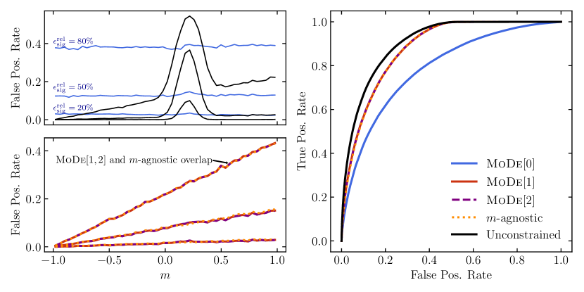
In this simple example, we can easily choose to only use information not explicitly indicative of mass by removing $x_{2}$ from $\mathcal{X}$. Figure 2 shows that the resulting mass agnostic classifier is linearly correlated with mass. Indeed, we ensured this via our choice of $x_{2}$, i.e. we configured this toy example such that the optimal classifier, the likelihood ratio, is linearly correlated with mass and obtained without the use of $x_{2}$. However, a classifier that enforces decorrelation must accept backgrounds 1 and 2 at equal rates to keep $p(s|m)$ flat, which as shown in Fig. 2 produces performance that is far from optimal. By relaxing the flatness constraint, MoDe[1] is able to reject background 2 at a higher rate, while producing the expected linear dependence on mass. This linear mass dependence, which will not sculpt out any fake peaks from the background, allows MoDe[1] to achieve better classification power than is possible using decorrelation. In this case, it is able to achieve the same performance as the optimal mass-agnostic classifier, since the optimal performance here is linear. Figure 2 shows that even though MoDe[2] is given the freedom to find quadratic mass dependence, it also produces the same optimal linear mass dependence in this case.

As discussed in Sec. 2, the MoDe package provides an even higher level of control over the response of a model, including allowing the analyst to define the maximum linear slope and to require that the quadratic dependence is monotonic. To demonstrate these features, we make the following minor change to the simple model:

$$x_{2}\to{\rm exp}(m)+2m.$$ (25)

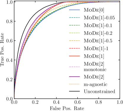
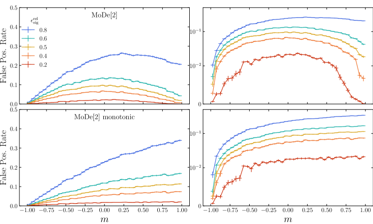
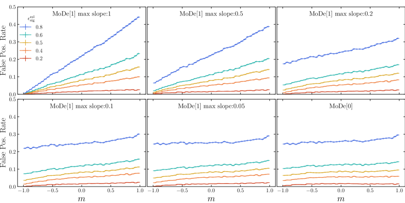
In this case, the optimal classifier is no longer linear. Figure 3 shows that here the additional freedom given to MoDe[2] does improve the classification performance. Figure 4 shows that the MoDe[2] solution does indeed have quadratic mass dependence. The MoDe[2] response is not monotonic by default, but we also show in Fig. 4 that we can apply such a constraint. As can be seen in Fig. 3, there is a small decrease in classification performance; whether this is acceptable is a problem-specific decision left to the analyst. Finally, Fig. 5 shows that the analyst can exert full control over the maximum linear slope. This could be desirable in cases where the signal mass is not known, and similar—but not necessarily equivalent—performance across the mass range is viewed as beneficial.

Figure 3: Same as the right panel of Fig. 2 but with the simple-model modification of Eq. (25). In addition, a monotonic version of MoDe[2] and several versions of MoDe[1] with constrained maximum slope values are also shown.

Figure 4: Top: False positive rate versus mass at various signal efficiencies for non-monotonic MoDe[2] on the modified simple-model example; see Eq. (25). Bottom: False positive rate for monotonic MoDe[2]. N.b., the right panels show the same curves as the left but on log scales.

Figure 5: Results for MoDe[1] on the modified simple-model example requiring various maximum slope values.

3.2 Boosted hadronic $W$ tagging

As mentioned in Sec. 1, highly lorentz boosted, hadronically decaying $W$ bosons commonly arise in extensions of the Standard Model. The boost causes the decay products of these bosons to be collimated in the lab frame and to be mostly captured by a single large-radius jet. Various features of the substructure of these jets can be used to distinguish the boosted bosons from generic quark and gluon jets.

A bump hunt is performed either in the mass of the $W$ candidate jet, $m_{J}$, or the mass of one $W$ candidate jet and another (possibly $W$ candidate) jet, $m_{JJ}$. The challenge with substructure classifiers is that they can introduce artificial bumps into the mass spectrum because substructure is correlated with the jet mass and the jet kinematic properties (which are related to $m_{JJ}$). For this reason, boosted $W$ tagging has become a benchmark process for studying decorrelation methods at the LHC.

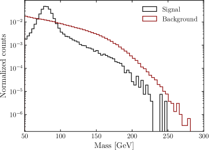
The simulated samples used in this section are the same as in Ref. DiscoFever (intended to emulate the study in Ref. ATL-PHYS-PUB-2018-014 ) and are briefly summarized here. In particular, boosted $W$ bosons (signal) and generic multijet (background) events are generated with Pythia 8.219 Sjostrand:2006za ; Sjostrand:2014zea and a detector simulation is provided by Delphes 3.4.1 deFavereau:2013fsa ; Mertens:2015kba ; Selvaggi:2014mya . Jets are clustered using the anti-$k_{t}$ algorithm Cacciari:2008gp with $R=1.0$ implemented in FastJet 3.0.1 Cacciari:2011ma ; Cacciari:2005hq . The selected jets for this study have 300 GeV $<p_{T}<$ 400 GeV and 50 GeV$<m_{J}<$ 300 GeV. Ten representative jet substructure features are computed for each jet and used for classification. This list is the same as in Ref. ATL-PHYS-PUB-2018-014 (based on Ref. ATLAS-CONF-2017-064 ) and includes the energy correlation ratios $C_{2}$ and $D_{2}$ Larkoski:2014gra , the $N$-subjettiness ratio $\tau_{21}$ Thaler:2010tr , the Fox-Wolfram moment $R_{2}^{\text{FW}}$ PhysRevLett.41.1581 , planar flow $\mathcal{P}$ Almeida:2008tp , the angularity $a_{3}$ Aad:2012meb , aplanarity $A$ Chen:2011ah , the splitting scales $Z_{\text{cut}}$ Thaler:2008ju and $\sqrt{d_{12}}$ Aad:2013ueu , and the $k_{t}$ subjet opening angle $KtDR$ CATANI1993187 . Detailed explanations of these features can be found in the references.

3.2.1 Classifier Details

MoDe and DisCo:

We use a simple 3-layer neural network with a similar architecture to that described in Ref. DiscoFever . However, unlike Refs. DiscoFever and ATL-PHYS-PUB-2018-014 , after each of the 3 fully connected 64-node layers, we use Swish activation ramachandran2017searching as it provides a notable performance increase. We also use a batch normalization layer after the first fully connected layer. The output layer has a single node with a sigmoid activation. Both MoDe and DisCo are trained with the ADAM optimizer DBLP:journals/corr/KingmaB14 using a 1cycle learning rate policy smith2018superconvergence with a starting learning rate of $10^{-3}$ and a maximum learning rate ($lr$) of $10^{-2}$, which is reached using a cosine annealing strategy loshchilov2017sgdr and decayed to $10^{-5}$ during the last few iterations. Momentum is cycled in the inverse direction from 0.95 to a minimum of 0.85. These hyperparameters were selected through a learning rate range test. Training is done using large batches of 10–20% of the training data. Note that large batch sizes do not necessarily make training more difficult especially when coupled with the 1cycle learning policy; see Ref. smith2017superconvergence .

Adversarial Decorrelation:

The same classifier used for MoDe and DisCo is trained against a Gaussian Mixture Network (GMN) Bishop94mixturedensity that parametrizes a Gaussian mixture model with 20 components, i.e. its outputs are the means, variances, and mixing coefficients of 20 normal distributions. We follow a similar adversarial setup to that referenced in Refs. ATL-PHYS-PUB-2018-014 and DiscoFever . We use one hidden layer with 64 nodes with ReLu activation connected to 60 output nodes. These outputs are then used to model the posterior probability density function $p_{\theta_{\mathrm{adv}}}(m|f(X)=s)$, where $\theta_{\mathrm{adv}}$ are the parameters of the GMN. The adversary is optimized by maximizing the likelihood of the data given by

$$L_{\mathrm{adv}}=\mathbb{E}_{s\sim f(X)}\mathbb{E}_{m\sim M|s}\left[-\log\,p_{\theta_{\text{adv}}}(m|s)\right].$$ (26)

The training procedure starts by training the classifier alone for 20 epochs with $lr=10^{-4}$ followed by 20 epochs of adversarial training only with $lr=5\cdot 10^{-3}$. Finally, both networks are trained simultaneously by optimizing the following loss function

$$\arg\min_{\theta_{\mathrm{class}}}\;\max_{\theta_{\mathrm{adv}}}\left[L_{\mathrm{class}(\theta_{\mathrm{class}})}-\lambda L_{\mathrm{adv}}(\theta_{\mathrm{class}},\theta_{\mathrm{adv}})\right],$$ (27)

where $\theta_{\mathrm{class}}$ and $\theta_{\mathrm{adv}}$ are the parameters of the classifier and the adversary, respectively. To control the classification-decorrelation trade-off, we vary $\lambda$ between 1 and 100. The non-convex nature of the loss makes training considerably more difficult; the hyperparameters must be chosen carefully.

3.2.2 Decorrelation

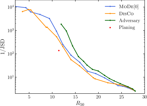
First, we will show that MoDe[0] achieves state-of-the-art decorrelation performance. Following Ref. DiscoFever , we quantify the classification and decorrelation performance using the following metrics: R50, the background rejection power (inverse false positive rate) at $50\%$ signal efficiency; and 1/JSD, where the Jensen-Shannon divergence (JSD) is a symmetrized version of the Kullback–Leibler divergence. Here, JSD is used to compare the mass distributions of backgrounds that pass and fail the classifier-based selections, with the relative entropy measured in bits.

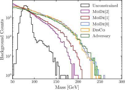
Figure 6 shows that, as expected, without imposing a strong constraint on mass decorrelation, the classifier learns to select samples near the $W$-boson mass, which sculpts a fake peak in the background. Figure 6 also shows that MoDe[0] successfully decorrelates its response from mass (if the decorrelation hyperparameter $\lambda$ is chosen to be sufficiently large). Figure 7 shows that the existing state-of-the-art decorrelation methods discussed in Sec. 2 perform similarly to MoDe[0] on this $W$-tagging problem. More precisely, as observed in Ref. DiscoFever , the adversary method performs slightly better, but is considerably more difficult to train, since it requires carefully tuning two neural networks against each other. The optimal solution is a saddle point, where the classification and adversarial losses are minimized and maximized, respectively, which makes the training inherently unstable. Conversely, both DisCo and MoDe[0] minimize convex loss functions, making their training robust and stable, and both only introduce one additional hyperparameter in the loss function. The performances of MoDe[0] and DisCo are comparable in these metrics (Appendix A shows that MoDe[0] is less resource intensive), though decorrelation is not our primary objective.

Figure 6: Left: Distributions of signal and background events without selection. Right: Background distributions at 50% signal efficiency (true positive rate) for different classifiers. The unconstrained classifier sculpts a peak at the $W$-boson mass, while other classifiers do not.

Figure 7: Decorrelation versus background-rejection power showing that MoDe[0] performs similarly to existing state-of-the-art decorrelation methods.

3.2.3 Beyond Decorrelation

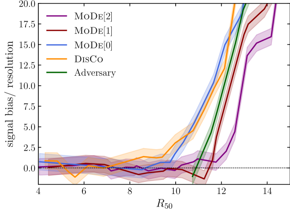
Moving beyond decorrelation the 1/JSD metric is no longer relevant. Figure 6 shows that neither MoDe[1] nor MoDe[2] sculpts a peaking structure in the background, but their 1/JSD values are small since neither seeks to decorrelate from the mass. Therefore, we replace the 1/JSD metric with the signal bias induced by the classifier selection, which is what actually matters when searching for resonant new physics. Specifically, we use the signal estimators obtained by fitting the selected background-only samples to a simple polynomial function as proxies for the signal biases. These are divided by their uncertainties such that values of roughly unity are consistent with no bias, while values significantly larger than unity indicate substantial bias that could result in false claims of observations.

Figure 8 shows that the DisCo and MoDe[0] decorrelation methods provide unbiased signal estimators for ${\rm R50}\lesssim 9$, which from Fig. 7 corresponds to $1/{\rm JSD}\gtrsim 1000$. While achieving higher decorrelation values is possible, this does not provide any tangible gains in the bump-hunt analysis. Figure 8 also shows that the flexibility to go beyond decorrelation provided by MoDe[1] and MoDe[2] results in achieving unbiased signal estimators at larger background-rejection power. This would directly translate to improved sensitivity in a real-world analysis. For example, since it is likely that only unbiased classifiers would be considered, Fig. 8 can be used to estimate the improvement in the signal cross-section sensitivity for the $W$-tagging analysis, which scales roughly like $\sqrt{R_{50}}$, using the classifier of each type with the largest $R_{50}$ value that is consistent with being unbiased. MoDe[1] and MoDe[2] provide roughly 5% improved sensitivity over the adversary method, which recall is considerably more difficult to train, and 10–20% improvements over the other decorrelation methods. We note, however, that how much is gained will strongly depend on the specifics of the problem, e.g., how large of a mass range is considered and whether the signal mass is known or if a scan in mass will be done.

Figure 8: Signal bias relative to resolution, which is roughly the square root of the background in the signal region, versus background-rejection power. The flexibility beyond simple decorrelation provided by MoDe[1] and MoDe[2] result in improved performance, i.e. larger rejection power.

4 Conclusions and Outlook

In summary, a key challenge in searches for resonant new physics is that classifiers trained to enhance potential signals must not induce localized structures. In particular, if classifiers can infer the mass of the parent resonance, then selecting signal-like events will simply pick out background events with a reconstructed mass near the target resonance mass creating an artificial structure in the background. Such structures could result in a false signal when the background is estimated from data using sideband methods. A variety of techniques have been developed to construct classifiers which are independent from the resonant feature (often a mass). Such strategies are sufficient to avoid localized structures, but are not necessary.

In this article, we presented a new set of tools using a novel moment loss function (Moment Decomposition or MoDe) which relax the assumption of independence without creating structures in the background. Using MoDe, analysts can require independence, linear dependence, quadratic dependence, etc. In addition, analysts can place bounds on the slope of the linear dependence, and restrict higher-order dependence to be monotonic. By allowing classifiers to be more flexible, we enhance the sensitivity to new physics without compromising the fidelity of the background estimation.

Code and Data

An implementation for MoDe in PyTorch as well as Keras/Tensorflow is available at https://github.com/okitouni/MoDe, along with example code used to produce the results in this article. The simulated $W$ and QCD samples are available from Zenodo at Ref. gregor_kasieczka_2020_3606767 .

Appendix A Scalability

Figure 9: Maximum memory usage and CPU time for different batch sizes of triples $(s_{i},m_{i},y_{i})$.

References

- (1) J. Button, G. R. Kalbfleisch, G. R. Lynch, B. C. Maglić, A. H. Rosenfeld and M. L. Stevenson, Pion-Pion Interaction in the Reaction , Phys. Rev. 126 (1962) 1858–1863.
- (2) ATLAS collaboration, G. Aad et al., Observation of a new particle in the search for the Standard Model Higgs boson with the ATLAS detector at the LHC, Phys. Lett. B 716 (2012) 1–29, [1207.7214].
- (3) CMS collaboration, S. Chatrchyan et al., Observation of a New Boson at a Mass of 125 GeV with the CMS Experiment at the LHC, Phys. Lett. B 716 (2012) 30–61, [1207.7235].
- (4) CMS collaboration, A. M. Sirunyan et al., Search for high mass dijet resonances with a new background prediction method in proton-proton collisions at 13 TeV, JHEP 05 (2020) 033, [1911.03947].
- (5) ATLAS collaboration, G. Aad et al., Search for new resonances in mass distributions of jet pairs using 139 fb-1 of collisions at TeV with the ATLAS detector, JHEP 03 (2020) 145, [1910.08447].
- (6) LHCb collaboration, R. Aaij et al., Searches for low-mass dimuon resonances, 2007.03923.
- (7) STAR collaboration, J. Adam et al., Pair invariant mass to isolate background in the search for the chiral magnetic effect in Au+Au collisions at = 200 GeV, 2006.05035.
- (8) ALICE collaboration, S. Acharya et al., J/ elliptic and triangular flow in Pb-Pb collisions at = 5.02 TeV, 2005.14518.
- (9) HPS collaboration, P. Adrian et al., Search for a dark photon in electroproduced pairs with the Heavy Photon Search experiment at JLab, Phys. Rev. D 98 (2018) 091101, [1807.11530].
- (10) CLAS collaboration, M. McCracken et al., Search for baryon-number and lepton-number violating decays of hyperons using the CLAS detector at Jefferson Laboratory, Phys. Rev. D 92 (2015) 072002, [1507.03859].
- (11) BESIII collaboration, M. Ablikim et al., Observation of the leptonic decay , Phys. Rev. Lett. 123 (2019) 211802, [1908.08877].
- (12) Belle-II collaboration, Search for Axion-Like Particles produced in collisions at Belle II, 2007.13071.
- (13) M. Frate, K. Cranmer, S. Kalia, A. Vandenberg-Rodes and D. Whiteson, Modeling Smooth Backgrounds and Generic Localized Signals with Gaussian Processes, 1709.05681.
- (14) A. J. Larkoski, I. Moult and B. Nachman, Jet Substructure at the Large Hadron Collider: A Review of Recent Advances in Theory and Machine Learning, Phys. Rept. 841 (2020) 1–63, [1709.04464].
- (15) D. Guest, K. Cranmer and D. Whiteson, Deep Learning and its Application to LHC Physics, 1806.11484.
- (16) K. Albertsson et al., Machine Learning in High Energy Physics Community White Paper, 1807.02876.
- (17) A. Radovic, M. Williams, D. Rousseau, M. Kagan, D. Bonacorsi, A. Himmel et al., Machine learning at the energy and intensity frontiers of particle physics, Nature 560 (2018) 41–48.
- (18) D. Bourilkov, Machine and Deep Learning Applications in Particle Physics, Int. J. Mod. Phys. A 34 (2020) 1930019, [1912.08245].
- (19) ATLAS collaboration, M. Aaboud et al., Performance of top-quark and -boson tagging with ATLAS in Run 2 of the LHC, Eur. Phys. J. C 79 (2019) 375, [1808.07858].
- (20) CMS collaboration, A. M. Sirunyan et al., Identification of heavy, energetic, hadronically decaying particles using machine-learning techniques, JINST 15 (2020) P06005, [2004.08262].
- (21) ATLAS Collaboration, Search for diboson resonances in hadronic final states in 139 fb-1 of collisions at TeV with the ATLAS detector, JHEP 09 (2019) 091, [1906.08589].
- (22) ATLAS Collaboration, Search for heavy diboson resonances in semileptonic final states in collisions at TeV with the ATLAS detector, 2004.14636.
- (23) CMS Collaboration, A multi-dimensional search for new heavy resonances decaying to boosted WW, WZ, or ZZ boson pairs in the dijet final state at 13 TeV, Eur. Phys. J. C 80 (2020) 237, [1906.05977].
- (24) CMS Collaboration, Combination of CMS searches for heavy resonances decaying to pairs of bosons or leptons, Phys. Lett. B 798 (2019) 134952, [1906.00057].
- (25) ATLAS Collaboration, Search for resonances decaying into a weak vector boson and a Higgs boson in the fully hadronic final state produced in protonproton collisions at TeV with the ATLAS detector, 2007.05293.
- (26) CMS Collaboration, Search for heavy resonances decaying into two Higgs bosons or into a Higgs boson and a W or Z boson in proton-proton collisions at 13 TeV, JHEP 01 (2019) 051, [1808.01365].
- (27) ATLAS Collaboration, Reconstruction and identification of boosted di- systems in a search for Higgs boson pairs using 13 TeV protonproton collision data in ATLAS, 2007.14811.
- (28) CMS Collaboration, Search for resonances decaying to a pair of Higgs bosons in the final state in proton-proton collisions at 13 TeV, JHEP 10 (2019) 125, [1904.04193].
- (29) CMS Collaboration, Search for a massive resonance decaying to a pair of Higgs bosons in the four b quark final state in proton-proton collisions at 13 TeV, Phys. Lett. B 781 (2018) 244–269, [1710.04960].
- (30) ATLAS Collaboration, Search for Higgs boson decays into a boson and a light hadronically decaying resonance using 13 TeV collision data from the ATLAS detector, 2004.01678.
- (31) ATLAS Collaboration, A search for resonances decaying into a Higgs boson and a new particle in the final state with the ATLAS detector, Phys. Lett. B 779 (2018) 24–45, [1709.06783].
- (32) ATLAS collaboration, G. Aad et al., Dijet resonance search with weak supervision using TeV collisions in the ATLAS detector, Phys. Rev. Lett. 125 (2020) 131801, [2005.02983].
- (33) ATLAS Collaboration, Search for light resonances decaying to boosted quark pairs and produced in association with a photon or a jet in proton-proton collisions at TeV with the ATLAS detector, Phys. Lett. B 788 (2019) 316, [1801.08769].
- (34) CMS Collaboration, Search for Low Mass Vector Resonances Decaying to Quark-Antiquark Pairs in Proton-Proton Collisions at , Phys. Rev. Lett. 119 (2017) 111802, [1705.10532].
- (35) CMS Collaboration, Search for low-mass resonances decaying into bottom quark-antiquark pairs in proton-proton collisions at 13 TeV, Phys. Rev. D 99 (2019) 012005, [1810.11822].
- (36) CMS Collaboration, Search for Low-Mass Quark-Antiquark Resonances Produced in Association with a Photon at =13 TeV, Phys. Rev. Lett. 123 (2019) 231803, [1905.10331].
- (37) CMS Collaboration, Search for low mass vector resonances decaying into quark-antiquark pairs in proton-proton collisions at 13 TeV, Phys. Rev. D 100 (2019) 112007, [1909.04114].
- (38) ATLAS Collaboration, Search for boosted resonances decaying to two b-quarks and produced in association with a jet at TeV with the ATLAS detector, ATLAS-CONF-2018-052 (2018) .
- (39) CMS Collaboration, Inclusive search for a highly boosted Higgs boson decaying to a bottom quark-antiquark pair, Phys. Rev. Lett. 120 (2018) 071802, [1709.05543].
- (40) G. Louppe, M. Kagan and K. Cranmer, Learning to pivot with adversarial networks, in Advances in Neural Information Processing Systems 30 (I. Guyon, U. V. Luxburg, S. Bengio, H. Wallach, R. Fergus, S. Vishwanathan et al., eds.), pp. 981–990. Curran Associates, Inc., 2017. 1611.01046.
- (41) J. Dolen, P. Harris, S. Marzani, S. Rappoccio and N. Tran, Thinking outside the ROCs: Designing Decorrelated Taggers (DDT) for jet substructure, JHEP 05 (2016) 156, [1603.00027].
- (42) I. Moult, B. Nachman and D. Neill, Convolved Substructure: Analytically Decorrelating Jet Substructure Observables, JHEP 05 (2018) 002, [1710.06859].
- (43) J. Stevens and M. Williams, uBoost: A boosting method for producing uniform selection efficiencies from multivariate classifiers, JINST 8 (2013) P12013, [1305.7248].
- (44) C. Shimmin, P. Sadowski, P. Baldi, E. Weik, D. Whiteson, E. Goul et al., Decorrelated Jet Substructure Tagging using Adversarial Neural Networks, 1703.03507.
- (45) L. Bradshaw, R. K. Mishra, A. Mitridate and B. Ostdiek, Mass Agnostic Jet Taggers, 1908.08959.
- (46) ATLAS collaboration, Performance of mass-decorrelated jet substructure observables for hadronic two-body decay tagging in ATLAS, Tech. Rep. ATL-PHYS-PUB-2018-014, CERN, Geneva, Jul, 2018.
- (47) G. Kasieczka and D. Shih, DisCo Fever: Robust Networks Through Distance Correlation, 2001.05310.
- (48) L.-G. Xia, QBDT, a new boosting decision tree method with systematical uncertainties into training for High Energy Physics, Nucl. Instrum. Meth. A930 (2019) 15–26, [1810.08387].
- (49) C. Englert, P. Galler, P. Harris and M. Spannowsky, Machine Learning Uncertainties with Adversarial Neural Networks, Eur. Phys. J. C79 (2019) 4, [1807.08763].
- (50) S. Wunsch, S. Jórger, R. Wolf and G. Quast, Reducing the dependence of the neural network function to systematic uncertainties in the input space, 1907.11674.
- (51) A. Rogozhnikov, A. Bukva, V. Gligorov, A. Ustyuzhanin and M. Williams, New approaches for boosting to uniformity, JINST 10 (2015) T03002, [1410.4140].
- (52) CMS collaboration, A deep neural network to search for new long-lived particles decaying to jets, Machine Learning: Science and Technology (2020) , [1912.12238].
- (53) J. M. Clavijo, P. Glaysher and J. M. Katzy, Adversarial domain adaptation to reduce sample bias of a high energy physics classifier, 2005.00568.
- (54) G. Kasieczka, B. Nachman, M. D. Schwartz and D. Shih, ABCDisCo: Automating the ABCD Method with Machine Learning, 2007.14400.
- (55) S. Chang, T. Cohen and B. Ostdiek, What is the Machine Learning?, Phys. Rev. D 97 (2018) 056009, [1709.10106].
- (56) J. M. Clavijo, P. Glaysher and J. M. Katzy, Adversarial domain adaptation to reduce sample bias of a high energy physics classifier, 2005.00568.
- (57) CMS collaboration, A. M. Sirunyan et al., A deep neural network to search for new long-lived particles decaying to jets, 1912.12238.
- (58) CMS collaboration, A. M. Sirunyan et al., Search for low mass vector resonances decaying into quark-antiquark pairs in proton-proton collisions at TeV, JHEP 01 (2018) 097, [1710.00159].
- (59) CMS collaboration, A. M. Sirunyan et al., Search for dark matter produced in association with a Higgs boson decaying to a pair of bottom quarks in proton–proton collisions at , Eur. Phys. J. C 79 (2019) 280, [1811.06562].
- (60) CMS collaboration, A. M. Sirunyan et al., Measurement and interpretation of differential cross sections for Higgs boson production at 13 TeV, Phys. Lett. B 792 (2019) 369–396, [1812.06504].
- (61) CMS collaboration, A. M. Sirunyan et al., Inclusive search for highly boosted Higgs bosons decaying to bottom quark-antiquark pairs in proton-proton collisions at 13 TeV, 2006.13251.
- (62) LHCb collaboration, R. Aaij et al., Amplitude analysis of the decay, 2009.00026.
- (63) LHCb collaboration, R. Aaij et al., A model-independent study of resonant structure in decays, 2009.00025.
- (64) LHCb collaboration, R. Aaij et al., Measurement of the -violating phase from decays in 13 TeV collisions, Phys. Lett. B 797 (2019) 134789, [1903.05530].
- (65) LHCb collaboration, R. Aaij et al., Search for a dimuon resonance in the mass region, JHEP 09 (2018) 147, [1805.09820].
- (66) LHCb collaboration, R. Aaij et al., Search for hidden-sector bosons in decays, Phys. Rev. Lett. 115 (2015) 161802, [1508.04094].
- (67) LHCb collaboration, R. Aaij et al., First observation of forward production in collisions at TeV, Phys. Lett. B 776 (2018) 430–439, [1709.03458].
- (68) LHCb collaboration, R. Aaij et al., Measurement of forward , and production in collisions at TeV, Phys. Lett. B 767 (2017) 110–120, [1610.08142].
- (69) H. Edwards and A. J. Storkey, Censoring representations with an adversary, in 4th International Conference on Learning Representations, ICLR 2016, San Juan, Puerto Rico, May 2-4, 2016, Conference Track Proceedings (Y. Bengio and Y. LeCun, eds.), 2016, 1511.05897.
- (70) Y. Ganin, E. Ustinova, H. Ajakan, P. Germain, H. Larochelle, F. Laviolette et al., Domain-adversarial training of neural networks, Journal of Machine Learning Research 17 (2016) 1–35, [1505.07818].
- (71) N. Mehrabi, F. Morstatter, N. Saxena, K. Lerman and A. Galstyan, A survey on bias and fairness in machine learning, 1908.09635.
- (72) A. Chouldechova and A. Roth, The frontiers of fairness in machine learning, 1810.08810.
- (73) L. de Oliveira, M. Kagan, L. Mackey, B. Nachman and A. Schwartzman, Jet-Images – Deep Learning Edition., JHEP 07 (2016) 069, [1511.05190].
- (74) G. J. Székely, M. L. Rizzo and N. K. Bakirov, Measuring and testing dependence by correlation of distances, Ann. Statist. 35 (2007) 2769–2794.
- (75) G. J. Székely and M. L. Rizzo, Brownian distance covariance, Ann. Appl. Stat. 3 (2009) 1236–1265.
- (76) G. J. Székely and M. L. Rizzo, The distance correlation t-test of independence in high dimension, J. Multivar. Anal. 117 (2013) 193–213.
- (77) G. J. Székely and M. L. Rizzo, Partial distance correlation with methods for dissimilarities, Ann. Statist. 42 (2014) 2382–2412.
- (78) A. Paszke, S. Gross, F. Massa, A. Lerer, J. Bradbury, G. Chanan et al., Pytorch: An imperative style, high-performance deep learning library, in Advances in Neural Information Processing Systems 32 (H. Wallach, H. Larochelle, A. Beygelzimer, F. d'Alché-Buc, E. Fox and R. Garnett, eds.), pp. 8024–8035. Curran Associates, Inc., 2019.
- (79) T. Sjöstrand, S. Mrenna and P. Z. Skands, PYTHIA 6.4 Physics and Manual, JHEP 05 (2006) 026, [hep-ph/0603175].
- (80) T. Sjöstrand, S. Ask, J. R. Christiansen, R. Corke, N. Desai, P. Ilten et al., An introduction to PYTHIA 8.2, Comput. Phys. Commun. 191 (2015) 159–177, [1410.3012].
- (81) DELPHES 3 collaboration, J. de Favereau, C. Delaere, P. Demin, A. Giammanco, V. Lemaitre, A. Mertens et al., DELPHES 3, A modular framework for fast simulation of a generic collider experiment, JHEP 02 (2014) 057, [1307.6346].
- (82) A. Mertens, New features in Delphes 3, J. Phys. Conf. Ser. 608 (2015) 012045.
- (83) M. Selvaggi, DELPHES 3: A modular framework for fast-simulation of generic collider experiments, J. Phys. Conf. Ser. 523 (2014) 012033.
- (84) M. Cacciari, G. P. Salam and G. Soyez, The anti- jet clustering algorithm, JHEP 04 (2008) 063, [0802.1189].
- (85) M. Cacciari, G. P. Salam and G. Soyez, FastJet User Manual, Eur. Phys. J. C72 (2012) 1896, [1111.6097].
- (86) M. Cacciari and G. P. Salam, Dispelling the myth for the jet-finder, Phys. Lett. B641 (2006) 57, [hep-ph/0512210].
- (87) ATLAS collaboration, Performance of Top Quark and W Boson Tagging in Run 2 with ATLAS, Tech. Rep. ATLAS-CONF-2017-064, CERN, Geneva, Aug, 2017.
- (88) A. J. Larkoski, I. Moult and D. Neill, Power Counting to Better Jet Observables, JHEP 12 (2014) 009, [1409.6298].
- (89) J. Thaler and K. Van Tilburg, Identifying Boosted Objects with N-subjettiness, JHEP 03 (2011) 015, [1011.2268].
- (90) G. C. Fox and S. Wolfram, Observables for the analysis of event shapes in annihilation and other processes, Phys. Rev. Lett. 41 (Dec, 1978) 1581–1585.
- (91) L. G. Almeida, S. J. Lee, G. Perez, I. Sung and J. Virzi, Top Jets at the LHC, Phys. Rev. D 79 (2009) 074012, [0810.0934].
- (92) ATLAS collaboration, G. Aad et al., ATLAS Measurements of the Properties of Jets for Boosted Particle Searches, Phys. Rev. D 86 (2012) 072006, [1206.5369].
- (93) C. Chen, New approach to identifying boosted hadronically-decaying particle using jet substructure in its center-of-mass frame, Phys. Rev. D 85 (2012) 034007, [1112.2567].
- (94) J. Thaler and L.-T. Wang, Strategies to Identify Boosted Tops, JHEP 07 (2008) 092, [0806.0023].
- (95) ATLAS collaboration, G. Aad et al., Measurement of splitting scales in events at TeV with the ATLAS detector, Eur. Phys. J. C 73 (2013) 2432, [1302.1415].
- (96) S. Catani, Y. Dokshitzer, M. Seymour and B. Webber, Longitudinally-invariant -clustering algorithms for hadron-hadron collisions, Nuclear Physics B 406 (1993) 187 – 224.
- (97) P. Ramachandran, B. Zoph and Q. V. Le, Searching for activation functions, 1710.05941.
- (98) D. P. Kingma and J. Ba, Adam: A method for stochastic optimization, in 3rd International Conference on Learning Representations, ICLR 2015, San Diego, CA, USA, May 7-9, 2015, Conference Track Proceedings (Y. Bengio and Y. LeCun, eds.), 2015, http://arxiv.org/abs/1412.6980.
- (99) L. N. Smith and N. Topin, Super-convergence: Very fast training of neural networks using large learning rates, 1708.07120.
- (100) I. Loshchilov and F. Hutter, SGDR: Stochastic gradient descent with warm restarts, 1608.03983.
- (101) L. N. Smith and N. Topin, Super-convergence: Very fast training of neural networks using large learning rates, 1708.07120.
- (102) C. M. Bishop, Mixture density networks, technical report, Birmingham, 1994.
- (103) G. Kasieczka and D. Shih, Datasets for boosted w tagging, Jan., 2020. 10.5281/zenodo.3606767.