Scintillation of PSR B1508+55 - the view from a 10000-km baseline

Abstract

We report on the simultaneous Giant Metrewave Radio Telescope (GMRT) and Algonquin Radio Observatory (ARO) observations at 550-750 MHz of the scintillation of PSR B1508+55, resulting in a $\sim$10,000-km baseline. This regime of measurement lies between the shorter few 100-1000 km baselines of earlier multi-station observations and the much longer earth-space baselines. We measure a scintillation cross-correlation coefficient of $0.22$, offset from zero time lag due to a $\sim 45$ s traversal time of the scintillation pattern. The scintillation time of 135 s is $3\times$ longer, ruling out isotropic as well as strictly 1D scattering. Hence, the low cross-correlation coefficient is indicative of highly anisotropic but 2D scattering. The common scintillation detected on the baseline is confined to low delays of $\lesssim 1\mu$s, suggesting that this correlation may not be associated with the parabolic scintillation arc detected at the GMRT. Detection of pulsed echoes and their direct imaging with the Low Frequency Array (LOFAR) by a different group enable them to measure a distance of 125 pc to the screen causing these echoes. These previous measurements, alongside our observations, lead us to propose that there are at least two scattering screens: the closer 125 pc screen causing the scintillation arc detected at GMRT, and a screen further beyond causing the scintillation detected on the GMRT-ARO baseline. We advance the hypothesis that the 125-pc screen partially resolves the speckle images on the screen beyond leading to loss of coherence in the scintillation dynamic spectrum, to explain the low cross-correlation coefficient.

1 INTRODUCTION

Interstellar scintillation (ISS) of pulsars has been used as a tool to study the ionized interstellar medium (IISM) and as a probe of pulsar magnetospheres. Pulsars, being unresolved at all radio wavelengths and emitting coherent radiation, are the best sources to study the IISM through their scintillation. Scintillation arises from constructive and destructive interference of the scattered rays, causing modulation of intensity in the time-frequency plane (see e.g. Cordes et al., 2006). Pulsar dynamic spectra often exhibit rich features caused by scintillation. The Fourier conjugate of the dynamic spectrum $I(t,\nu)$, where $t$ is time and $\nu$ is frequency, is called the conjugate spectrum, squaring which gives the secondary spectrum $S(f_{\mathrm{D}},\tau)=|\tilde{I}(f_{\mathrm{D}},\tau)|^{2}$, where $f_{\mathrm{D}}$ is the differential Doppler frequency and $\tau$ is the differential delay. In simple words, the secondary spectrum is the two-dimensional power spectrum of the intensity dynamic spectrum.

There has been considerable evolution in our understanding of interstellar scintillation in the last two decades. Our currently held view owes its beginnings to the discovery of parabolic scintillation arcs (Stinebring et al., 2001) in the secondary spectra of pulsars, challenging the notion of a largely volume-filling medium that had been posited as the origin for scattering. The presence of thin, well-defined, parabolic features in the secondary spectra of several pulsars (Hill et al., 2003; Cordes et al., 2006) means that highly anisotropic scattering occurs in localized regions along the line of sight. Evidence for anisotropic scattering came from direct mapping, by Brisken et al. (2010), of the scattered images on the sky aided by the resolving power of scintillation, far exceeding what is possible through conventional VLBI: they found a densely packed series of point-like scattered images of the pulsar, aligned roughly along a straight line, with the magnifications and number of speckles tapering off on either side of the line of sight. The separations between the speckle images on the screen range between $\sim 0.1$ and $\sim 10$ AU, the scales at which irregularities are thought to exist on the screen. These speckle images hint at a filamentary structure or structures in the IISM as the locales for the anisotropically scattered images.

In a scenario involving roughly spherical lenses, the high electron overdensities would translate into physically untenable overpressured regions, ruling out a volume-filling turbulent medium. To circumvent this difficulty, Pen & Levin (2014) advance a model where they invoke very thin plasma reconnection sheets confined between regions of misaligned magnetic fields. Perturbations propagate as Alfvèn-like surface waves, the amplitudes of which are very small in relation to the extent of the sheet. These sheets extend for several hundred AU but are highly inclined with the line of sight, causing extremely high projected local overdensities by virtue of which they have very high lensing potential. This model convincingly explains the observed anisotropic scattering reported by Brisken et al. (2010). If these structures persist in the sheets over long periods of time (compared to typical observing durations), as suggested by the Pen & Levin 2014 model, the images would appear to move relative to the pulsar due to the relative motion of the pulsar and the reconnection sheet. Earlier work by Hill et al. (2005) indeed measured uniform motion of the arclets along the main parabola suggesting that these features remain practically stationary in the screen as the pulsar moves behind it. Simard & Pen (2018) further analyze this model quantitatively to study the expected motion of the lensed images, effectively predicting their positions and magnifications in future time and out-of-band frequencies. Lensed images in the reconnection sheet model are caused by wave crests, each of which can be described by a single parameter. This facilitates a completely deterministic treatment of each lensed image, allowing a posteriori prediction of scintillation.

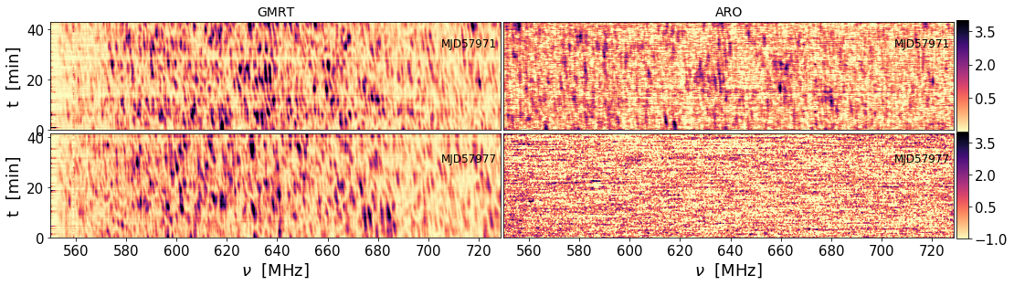
Figure 1: The dynamic spectra for B1508+55 from the two observing sessions at GMRT and ARO are shown here, between 550 and 730 MHz. Each pixel is $15P_{0}\times 293$ kHz. The colour scale in all the dynamic spectra ranges -1 to 4. The S/N of the ARO dynamic spectrum on MJD57977 is very poor because of a tracking malfunction. Only the first $\sim 40$ minute scan from the GMRT on MJD57977 is shown here.

1.1 PSR B1508+55

The pulsar we study in this paper is B1508+55, which has among the highest measured proper motion velocities, moving at $963^{+61}_{-64}$ km s^-1 south east and a measured parallax distance of $2.1\pm 0.1$ kpc (Chatterjee et al., 2009). Earlier observations of this pulsar (Stinebring, 2007) show thick horizontal streak-like features instead of parabolic reverse arclets in the secondary spectrum, besides straggler arclets that are not strictly aligned with the parabolic locus. An extra pulse component was initially detected with the German Long Wavelength Consortium (GLOW) telescopes (Oslowski et al., in prep.). Follow-up observations revealed that this component is approaching the main pulse, subsequently identified to be likely of an ISM origin. Further LOFAR observations have now revealed the presence of multiple images (Wucknitz, 2019) roughly aligned along the proper motion vector, suggesting that the pulsar is moving towards perhaps linearly aligned refracting structures. Bansal et al. (2020) report the detection of these echoes at frequencies below 100 MHz.

Given the peculiar thick-arc nature of the secondary spectrum and the imaging of the echoes, the two main goals in this work are: (i) to measure the scintillation time and the scintillation pattern delay on an orthogonal pair of long baselines at 650 MHz using dual station simultaneous observations in the 550-750 MHz band and (ii) to measure the correlation coefficient along the baselines and infer if the scattered image is one- or two-dimensional.

1.2 Thin screen scattering

It is useful to have a brief perspective of localized thin screen scattering to aid in some of the discussion in later sections. Definitions of quantities used throughout the remainder of this paper are in order: if $s$ is the fractional distance from the pulsar at which the screen is located, i.e. $s=1-d_{\mathrm{scr}}/d_{\mathrm{psr}}$, we define the effective distance and effective velocity as

$$D_{\mathrm{eff}}=\frac{1-s}{s}d_{\mathrm{psr}}$$ (1)

and

$$\mathbf{V}_{\mathrm{eff}}=\frac{1-s}{s}\mathbf{V}_{\mathrm{psr}}+\mathbf{V}_{\mathrm{obs}}-\frac{1}{s}\mathbf{V}_{\mathrm{scr}}$$ (2)

where $d_{\mathrm{psr}}$ is the distance to the pulsar from the observer and $d_{\mathrm{scr}}$ is the distance to the scattering screen. $\mathbf{V}_{\mathrm{psr}}$, $\mathbf{V}_{\mathrm{obs}}$ and $\mathbf{V}_{\mathrm{scr}}$ are the velocities of the pulsar, observer and the screen respectively. The equations and the formalism presented here apply strictly to one-dimensional (1D) scattering.

Since the scattered ray suffers an additional path length, it picks up a differential time delay $\tau$ proportional to the square of the angular displacement from the line of sight, $\theta$ (Stinebring et al., 2001; Hill et al., 2003; Cordes et al., 2006):

$$\tau=\frac{D_{\mathrm{eff}}}{2c}\theta^{2}.$$ (3)

Due to the uniform motion of the pulsar and the stationarity of the images on the screen (assuming that the lifetime of substructure on the screen is much longer than an observation), the differential delay changes at a rate proportional to the effective velocity, i.e. linear in angular separation between pairs of images,

$$f_{\mathrm{D}}=\nu\frac{d\tau}{dt}=\mn@boldsymbol{\theta}\cdot\mathbf{V}_{\mathrm{eff}}/\lambda$$ (4)

from which it follows that

$$\tau=\eta f_{\mathrm{D}}^{2},$$ (5)

where $f_{\mathrm{D}}$ is the differential Doppler frequency and $\eta$ is the curvature of the parabolic arc:

$$\eta=\frac{\lambda^{2}}{2c}\ \!\frac{D_{\mathrm{eff}}}{|\mathbf{V}_{\mathrm{eff}}|^{2}\ \!\mathrm{cos}^{2}\alpha_{s}}.$$ (6)

$\alpha_{s}$ is the angle that the line of scattered images, which we henceforth call the scattering axis, makes with the effective velocity vector $\mathbf{V}_{\mathrm{eff}}$. The scintillation pattern, therefore, always moves along the scattering axis opposite to the direction of the projected effective velocity vector as seen by an observer on Earth. The curvature is degenerate in the effective distance $D_{\mathrm{eff}}$ and the effective velocity $\mathbf{V}_{\mathrm{eff}}$, precluding an independent measurement of both the quantities without explicit or implicit assumptions. Single station measurements of the curvature are therefore generally used with approximate effective velocities to estimate screen distances. A common assumption is that the largest contribution to the effective velocity accrues from the pulsar’s proper motion velocity (see e.g. Stinebring et al., 2001). Using a pair of radio telescopes, the apparent speed of the scintillation pattern along that baseline, $V^{\mathrm{app}}_{\mathrm{ISS}}$, can be measured. An independent measurement of the full 2D velocity of the scintillation pattern, measured using scintillation pattern traversal times between multiple stations observing simultaneously, would hence break the degeneracy between $D_{\mathrm{eff}}$ and $\mathbf{V}_{\mathrm{eff}}$.

2 OBSERVATIONS AND DATA

2.1 Simultaneous wideband observations

Observations of B1508+55 were carried out in two sessions in August 2017 simultaneously with the Giant Metrewave Radio Telescope (GMRT) and the Algonquin Radio Observatory (ARO) 46-m telescope. The GMRT observations were made with the 500-850 MHz Band-4 wideband feed, which were deployed on 15 antennas at the time. These feeds are now available on all 30 antennas and comprise one of the six wavebands of the upgraded GMRT (uGMRT; Gupta et al. 2017). We used the GPU-based GMRT Wideband Backend (GWB; Reddy et al. 2017) to process 550-750 MHz of Band-4. For the observations we report here, the GWB was deployed as a phased-array beamformer, in which voltages from the antennas are summed in phase before detection and sub-integration. The GWB was configured to split the 200-MHz bandwidth into 8192 channels to give a frequency resolution of 24.4 kHz, and a time resolution of 262.144 $\mu$s.

The ARO 46m dish, although not primarily an astronomical facility at present, is equipped with a 400-800 MHz feed designed and mass produced for the Canadian Hydrogen Intensity Mapping Experiment (CHIME). The entire band is digitized utilizing the bandpass sampling technique and recorded as baseband voltages with 1024 channels, implemented using a polyphase filter bank (Recnik et al., 2015).

We chose to observe on two different days, at LSTs separated by 6 hours, to realize a pair of orthogonal baselines aided by the high declination of the pulsar. It is sufficient that the scattering geometry is similar on both of the days. The exigent scheduling constraints at the GMRT meant that the closest such pair of observing sessions would be spaced $\sim 150$ hours apart.

In the first observing session on 2017-August-06 (MJD57971), B1508+55 was observed approximately for 45 minutes with the GMRT (of the one hour allocated on the day) and ARO simultaneously when the source was at an hour angle of -5h at the GMRT. The pulsar is circumpolar at ARO.

Observations of the second session on 2017-August-12 (MJD57977) commenced at a local sidereal time (LST) 6 hours later than on the first day and continued for 3 hours at both telescopes. Unfortunately the ARO 46m drive system malfunctioned and mistracked the source co-ordinates, rendering the data entirely unusable. However, at the GMRT, observations were carried out for the full 3 hours allocated, resulting in a total of 3 $\sim 40$-minute scans. Only the first $\sim 40$-minute scan is shown in Figure 1. The details of the observations are summarized in Table 1.

Table 1: Details of the observations of B1508+55 with the GMRT and ARO. $P_{0}$ is the period of B1508+55.

Setup	GMRT	ARO
Band(MHz)	550-750	400-800
Scan start
MJD57971	8:24:50 UTC	7:30:25 UTC
MJD57977	14:20:00 UTC	14:00:00 UTC
Scan stop
MJD57971	9:10:02 UTC	9:41:40 UTC
MJD57977	17:31:21 UTC	18:05:00 UTC
Number of channels	8192	1024
Native time resolution	262.144 $\mu$s	2.56 $\mu$s
Final time resolution ($t_{\mathrm{s}}$)	262.144 $\mu$s	$P_{0}/128$
Mode	Phased array intensity	Baseband voltage

2.2 Data reduction

The channelized GMRT data were dedispersed with the DM of 19.6191 pc cm^-3. Next, the band-averaged data were folded at the the period of the pulsar over $P_{0}/t_{\mathrm{s}}$ bins to determine the “on” phase. Then, for each single pulse for every channel, the mean of the “off” pulse was subtracted and the result divided again by the mean “off” pulse, to establish bandpass correction and to obtain the dynamic spectrum. Finally, the dynamic spectrum was normalized by dividing by its mean and subtracting unity. This final data product is used for computing the modulation index.

The ARO dynamic spectrum was similarly obtained after sub-integrating the pulse to 128 phase bins across the period. Since B1508+55 exhibits large pulse-to-pulse flux variability, we visually aligned the band-averaged pulse series to determine the clock offset between GMRT and ARO on MJD57971.

3 RESULTS

3.1 Dynamic and Secondary Spectra

The dynamic spectra of the GMRT and ARO from both sessions of the observations of B1508+55 are shown in Figure 1. Frequencies above 730 MHz are excluded from our analysis owing to severe mobile communication RFI at ARO. The autocorrelation of the normalized dynamic spectrum at zero time and frequency lag is hence the modulation index squared $m^{2}$ by definition (Johnson & Gwinn, 2012):

$$m^{2}=\frac{\langle(I-I_{n})^{2}\rangle}{\langle I-I_{n}\rangle^{2}}-1$$ (7)

where $I$ is the intensity time series and $I_{n}$ is the ‘off-pulse’ intensity time series which contains the receiver noise.

Due to their superior S/N, we will restrict our discussion of the secondary spectra to the GMRT observations. The secondary spectra for MJD57971 and MJD57977 are both shown in Figure 2. The native frequency resolution of the dynamic spectra is $\sim 24.4$ kHz; the highest delay in the secondary spectrum is thus 20.48 $\mu$s. There are several salient features to note: on both days, a substantial fraction of the power in scintillation is confined to $\lesssim$ 5 $\mu$s; at smaller delays, the lack of a clearly discernible parabolic feature complicates estimating the curvature. A striking absence of clear, well-defined reverse arclets, useful in identifying apexes through which to fit the main parabola, exacerbates the problem. The most notable difference between the two days is the systematic shift in the features identified with markers.

A simple approximation for the total shift in $f_{\mathrm{D}}$, valid when the curvature of the putative parabola has undergone no change, is given by

$$\Delta f_{\mathrm{D}}=\frac{\Delta t}{2\eta\nu}$$ (8)

which allows us to track isolated features along the main parabola in the secondary spectrum that correspond to interference between the lensed images and the line-of-sight ray from the pulsar as it moves behind the screen. Features in the parabola always move from negative through zero to positive Doppler frequencies: the delay decreases on the head-side and increases on the tail-side as the pulsar moves with respect to the stationary images.

We use different trial values for $\eta$ in eqn. 8 to determine the total shift in the differential Doppler frequency ($\Delta f_{\mathrm{D}}$). We identify the curvature ($\eta=0.76$ s³) that best predicts the net motion of the isolated arclet-like features. The markers identify those features that moved $\Delta f_{D}=0.546$ mHz between the two observing sessions. Similar motion of apexes of reverse arclets has been measured empirically by Hill et al. (2005) for B0834+06.

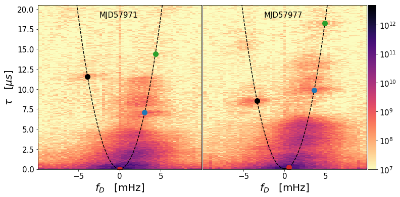
Figure 2: GMRT secondary spectra of B1508+55 on MJD57971 and MJD57977, obtained from the dynamic spectra shown in Figure 1. The markers indicate the positions of the features that have moved by an amount $\Delta f_{D}=0.546$ mHz, from which the curvature of the parabola $\eta=0.76$ s³ is estimated.

The qualitative similarities with earlier observations of this pulsar (Stinebring, 2007), such as the thick horizontal streak-like features instead of reverse arclets, as well as stragglers that stray from the parabolic locus, are unmistakable. Gwinn (2019) discusses the effects of wideband observations on the secondary spectrum: averaging over a large band causes a continuum shift in the curvature, resulting in thick streak-like features along the differential Doppler frequency. Wideband pulse intensity modulation could as well lead to smearing of features along thee Doppler frequency axis. However, we have confirmed that neither is the case with our observations of B1508+55 by a few independent means: (i) we weighted the dynamic spectrum by a two-dimensional Hanning window to obtain the secondary spectrum, (ii) we binned the dynamic spectrum 60$\times$ in time (i.e. 60$P_{0}$), (iii) we inspected the secondary spectra obtained over a much narrower subband ($\sim 25$ MHz), and (iv) we corrected for the wide bandwidth by linearly scaling the dynamic spectrum along the frequency axis, normalized for the reference frequency, followed by a discrete Fourier transform, to concentrate the power on the reference parabola. The horizontal streak-like features persisted in all the above cases, suggesting that this is an intrinsic feature of the scintillation of B1508+55 at these frequencies.

3.2 Cross-correlation of scintillation

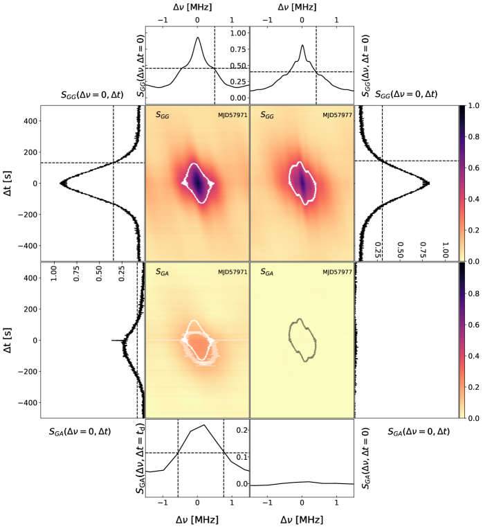
Figure 3: Autocorrelation of scintillation dynamic spectra of GMRT and GMRT-ARO cross-correlation of scintillation dynamic spectra. The top row of the 2D panels shows respectively the autocorrelation of the GMRT dynamic spectra $S_{\mathrm{GG}}$ on MJD57971 and MJD57977. The bottom row of the 2D panel shows the corresponding cross-correlation of GMRT-ARO scintillation dynamic spectra, $S_{\mathrm{GA}}$. The white contours in the top row are at half-maximum of the respective autocorrelation peaks while they are overlaid on the cross-correlations in the bottom 2D panel. The peak of the cross-correlation is offset $\sim$ -45s from zero lag in time. The peripheral plots are cuts of the auto- and cross-correlations through $\Delta\nu$ and $\Delta t$ where the 2D function peaks, from which we measure the scintillation bandwidth (half-width at half-maximum) and scintillation time (half-width at 1/$e$) listed in Table 2.

Each pixel of the raw GMRT dynamic spectrum is $P_{0}\times 200/8192$ MHz, and of the ARO dynamic spectrum is $P_{0}\times 400/1024$ MHz. We therefore bin the GMRT dynamic spectrum to the same resolution as that of ARO ($16\times$). One of the dynamic spectra is shifted along the time axis to reverse the relative clock-offset between the observatories. The dynamic spectra, each with 1024 channels across the 550-750 MHz band, are then transformed to their respective conjugate spectra and cross-multiplied according to (9), and transformed back to give the real-valued cross-correlation function (CCF) between the pair of dynamic spectra. The autocorrelation function (ACF) of the GMRT dynamic spectra are similarly obtained, but retaining the native frequency resolution. Figure 3 shows the 2D GMRT ACF and 2D GMRT-ARO CCF, along with the time- and frequency-lag cuts in the peripheral panels. The ARO ACFs are much noisier due to the significantly poorer S/N of the dynamic spectra, and are not shown here.

Figure 4: The GMRT-ARO difference dynamic spectrum for B1508+55 on MJD57971. The normalized ARO dynamic spectrum, shifted by the measured scintillation delay, has been subtracted from the normalized GMRT dynamic spectrum, showing the residual scintillation at GMRT and ARO.

We apply the arguments of Johnson & Gwinn (2012) to determine the true correlation coefficient from the modulation index squared. The modulation index at zero temporal and spectral lag has contributions from the intrinsic pulse variability and noise. We therefore interpolate the values at small non-zero spectral and temporal lags through zero lag to determine the correlation coefficient. Note that the autocorrelation coefficient thus obtained from non-zero temporal lags is free from the inherent bias introduced by intrinsic pulse variability (Johnson & Gwinn, 2012). The cross-correlation coefficient of the dynamic spectra from GMRT and ARO at zero temporal lag has the pulse variability contribution, but the peak of the cross-correlation shifts to a non-zero temporal lag due to the delay in the arrival of the scintillation pattern in one of the telescopes.

The scatter broadening ($\tau_{\mathrm{sc}}$) expected from the measured scintillation bandwidth is $\lesssim 1\mu$s, which is much smaller than the $\sim 2.6$ms time resolution of the recorded beam. We notice two conspicuous differences between the two GMRT 2D ACFs: first, the peak feature is narrower in frequency lag and, second, a small but perceptible rotation of the major axis on the second day with respect to the first. The structure in the frequency-lag ACF is evidence for multiple fringe spacings, corresponding to the many distinct islands of power in the GMRT secondary spectra shown in Figure 2.

The normalized CCF peak on MJD57971 is $\rho=0.22\pm 0.01$, which is in the same units as the ACF ($m^{2}=0.91\pm 0.01$), allowing for a meaningful and self-consistent comparison. There is no detectable correlation on MJD57977. The cross-correlation of $\sim 20\%$ is a crucial and a significant measurement. This is not entirely unexpected as, even visually, the dynamic spectra look different between GMRT and ARO on MJD57971 in Figure 1. Figure 4 shows the presence of residual scintillation at both ARO and GMRT, which underpins the low cross-correlation coefficient.

3.3 Scintillation delay on the baseline

We notice that the peak of the cross-correlation in Figure 3 is offset from zero-lag. This lag can also be robustly estimated by measuring the corresponding phase gradient in the Fourier plane.

For dynamic spectra $I_{\mathrm{G}}(\nu,t)$ and $I_{\mathrm{A}}(\nu,t)$ observed at the GMRT and ARO respectively, we obtain the quantity

$$\tilde{S}_{\mathrm{GA}}(\tau,f_{\mathrm{D}},\mathbf{b})=\tilde{I}_{\mathrm{G}}(\tau,f_{\mathrm{D}})\times\tilde{I}^{\ast}_{\mathrm{A}}(\tau,f_{\mathrm{D}}),$$ (9)

which Simard et al. (2019a) call the intensity cross secondary spectrum, where $\tilde{I}$, the 2D Fourier Transform (2DFT) of $I$, is called the conjugate spectrum (Brisken et al., 2010).

Figure 5 shows the magnitude and phase of the cross secondary spectra. We detect a phase gradient at $|\tau|\lesssim 1.0\mu s$ on MJD57971 and none on MJD57977, the latter due to a telescope malfunction at ARO.

The phase gradient $d\Phi/df_{\mathrm{D}}$ corresponds to a time delay in the arrival of the scintillation pattern in one telescope with respect to the other:

$$t_{\mathrm{d}}=\frac{1}{2\pi}\frac{d\Phi}{df_{\mathrm{D}}}$$ (10)

Figure 6 shows the delay-averaged phase across Doppler frequency measured on MJD57971. The errors on each point have been propagated from the standard deviation of the real and imaginary parts. The solid line is the inverse noise variance weighted fit to the gradient, the slope of which is $d\Phi/df_{\mathrm{D}}=0.285\pm 0.029$ rad mHz^-1. The error derived from the covariance matrix of the fit parameters is only 0.016 rad mHz^-1. The small error is not surprising given the tiny error bars on the points in blue. However, we expect the errors to be slightly higher owing to uncalibrated systematics: a conservative error of 10% is reasonable. This gradient translates into a scintillation pattern arrival delay of $t_{\mathrm{d}}=45.3\pm 4.5$ s, the pattern arriving earlier at the GMRT. Table 2 additionally lists the baseline vectors, pulsar proper motion and Earth velocity vectors and their relative orientations. The apparent speed of scintillation along the baseline is thus $220\pm 22\ \mathrm{km\ \!s^{-1}}$, which is an upper limit to the true sicntillation pattern velocity in the absence of a full 2D measurement of the scintillation pattern motion.

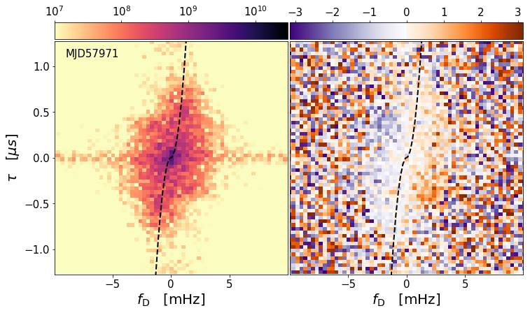
Figure 5: The log magnitude and phase (in radians) of the cross secondary spectrum of scintillation of B1508+55 on MJD57971. The parabola $\tau=\mathrm{sgn}(f_{\mathrm{D}})\ \!\eta\ \!f_{\mathrm{D}}^{2}$ for $\eta=0.76$ s³ is overlaid on the cross secondary spectral magnitude and phase.

Table 2: Measured parameters. The apparent scintillation speed measured on the baseline is negative as it is opposite in direction to the pulsar’s proper motion and hence the effective velocity. The baseline and velocity components are along $\mathbf{u}$ and $\mathbf{v}$ directions.

Parameter	MJD57971	MJD57977
Correlation coefficient ($m^{2}$)	$0.91\pm 0.01$	$0.80\pm 0.01$
Scintillation bandwidth (kHz)	500	410
Scintillation time (s)	$132\pm 3$	$145\pm 3$
Baseline length (km)	9974.3	10468.0
Baseline vector ($\times 1000$ km)	(-4.2, -9.0)	(9.7, -4.0)
Pulsar PM angle with BL	25∘	120∘
PM component along baseline (km s-1)	876	-437
Earth velocity vector (km s-1)	(2.7, 27.9)	(-0.3, 28.2)
Component along baseline (km s-1)	-26	-11
Apparent scintillation speed (km s-1)	$-220\pm 22$	NA
along baseline

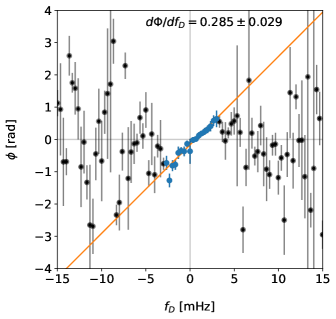
Figure 6: The delay-averaged phases for $\tau\!\!>\!\!0\ \!\mu$s against the differential Doppler frequency obtained from the cross secondary spectrum on MJD57971. The black points represent the measurement, while only the blue points have been included for determining the fit, shown by the solid orange line.

4 ASSUMPTIONS FOR A SIMPLE INTERPRETATION

4.1 Arc curvature

Our first assumption is that the curvature of the forward parabola does not change between the two epochs of observations, as they are only separated by 150 hours. The extrema of annual modulation of scintillation occurs six months apart. As a fraction of this duration, 150 hours is only 3.4%. The curvature of the forward parabola is measured to be $\eta=0.76\ \mathrm{s}^{3}$. While absence of clearly marked reverse arclets precludes fitting a parabola through their apexes, the best fit curvature parameter is estimated from the reflex motion of the thick arclet-like features. Besides, we rely on identifying the same arclet feature to measure the net displacement along the Doppler axis, which constrains how far apart such measurements are made. For a close pair of adjacent measurements, one can hence always assume $d\eta/dt=0$ and still reliably measure the annual modulation of the curvature with regularly spaced observation pairs. The full equation, however, is easily derived:

$$\frac{df_{\mathrm{D}}}{dt}=\frac{1}{2\eta\nu}\left(1-f_{\mathrm{D}}\nu\frac{d\eta}{dt}\right).$$ (11)

The simple model of Section 1.2 is necessary only to describe the curvature parameter $\eta$. In a two-screen model, it may apply only to the closer screen, or the "scintillation-arc screen" which produces the fringes in the dynamic spectrum and equivalently the parabola in the secondary spectrum.

4.2 Screen locations

It is possible to obtain limits on the screen locations even with the single beaseline measurement, but under certain assumptions that may be contrived. For example, one would have to assume that the screen makes a negligible contribution to the effective velocity. Implicitly, this would considerably bias the distance of a very nearby screen while screens closer to the pulsar are more immune to the approximation. We would hence defer any estimates of the location(s) of the scattering screens pending a full 2D scattering measurement.

In addition, it is unknown from these measurements if the $\eta=0.76\ \mathrm{s}^{3}$ is the same screen at 125 pc (Wucknitz, 2019) that causes the echo. More observations are required to establish this independently.

4.3 Scintillation pattern arrival time delay

The scintillation pattern arrival delay is a standalone measurement that holds without recourse to any restrictive assumptions about scattering geometry (e.g. Slee et al., 1974). Especially, we note that there arises no need to invoke anisotropic scattering, as the minimum assumption required to obtain the delay is a frozen screen approximation (see e.g. Smirnova et al., 2014, for the algebra), where the diffraction pattern due to the scattering screen is fixed in space sampled by the motion of the observer in an appropriate reference frame.

5 IMPLICATIONS

The main results of this paper are threefold: (i) the curvature of the parabolic arc of $\eta=0.76\ \mathrm{s}^{3}$, (ii) the time delay of arrival of the scintillation pattern at the two telescopes of $\Delta t_{\mathrm{d}}=45.3$ s and (iii) the low scintillation correlation of $\rho=0.22$ on the long baseline. We discuss their implications under the assumptions stated above.

Figure 7 shows the orientation of the GMRT-ARO baseline on MJD57971 and MJD57977 as solid lines, along with the velocity vectors of the Earth’s motion rotated to the $uvw$ co-ordinates; only the $u,v$ components are shown with dotted lines. The $w$-component is directed upwards and normal to the $uv$ plane. The components of the pulsar’s velocity in the right ascension and declination directions are computed from the proper motion for the distance $d_{\mathrm{psr}}$=2.1 kpc (Chatterjee et al., 2009).

5.1 Multiple scattering screens: possible scenarios

One of two possibilities could be considered: (1) the measurement of $\Delta t_{\mathrm{d}}=45.3$ s, or the equivalent $V^{\mathrm{app}}_{\mathrm{ISS}}=220$ km s^-1, is not associated with the $\eta=0.76$ s³ parabola at all, hinting at the presence of a second scattering screen, (2) if instead it is indeed associated with the $\eta=0.76$ s³ parabola, scattering beyond 1 $\mu$s is possibly resolved out by the baseline.

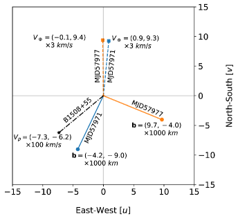
Figure 7: The orientation of the pulsar’s proper motion vector, the Earth’s motion vectors and the baseline vectors on MJD57971 and MJD57977 in the $u$ and $v$ directions.

We take note of an independent measurement of the distance to a scattering screen using LOFAR. These VLBI observations were carried out to map the pulsed echoes approaching the main pulse. Direct VLBI imaging of these echoes has revealed that they are aligned along the pulsar’s proper motion vector (Wucknitz, 2019), i.e. $\alpha_{s}\sim 0^{\circ}$ is a reasonable approximation. They also measure the distance to the screen of $d_{\mathrm{scr}}\sim 125$ pc. While these pulses were detected in the LOFAR observations, we do not detect them in the GMRT 550-750 MHz observations. Additionally, Bansal et al. (2020) measure a distance of $\sim 251$ pc to a lens based on their observations of B1508+55 at frequencies < 100 MHz.

5.1.1 Is the scintillation delay associated with the LOFAR echo screen?

For $d_{\mathrm{scr}}=125$ pc (Wucknitz, 2019), the effective velocity of scintillation from such a screen, if it is associated with the $\eta=0.76$ s³ parabola, is $|\mathbf{V}_{\mathrm{eff}}|\sim 47$ km s^-1. If the apparent scintillation pattern velocity of $V_{\mathrm{ISS}}^{\mathrm{app}}$ = 220 $\mathrm{km\ s^{-1}}$ is associated with the echo, then $\alpha_{s}=0^{\circ}$, and its effective velocity should be $V_{\mathrm{ISS}}^{\mathrm{app}}\mathrm{cos}\alpha_{\mathrm{\bf b}}$ = 200 km s^-1 (see Figure 8).

If the LOFAR measurement is therefore associated with the $\eta=0.76$ s³ parabola, it certainly hints at the presence of a second screen, whose location is unknown but likely closer to the observer than the pulsar, beyond the 125-pc screen and not associated with the $\eta=0.76$ s³ parabola. In that case, it is this second screen we detect on the MJD57971 baseline. The scintillation delay measured on the GMRT-ARO baseline is hence not associated with the LOFAR echo. However, we cannot conclusively establish, but can only propose, that the 125-pc LOFAR echo screen causes the $\eta=0.76$ s³ parabola in the GMRT secondary spectra.

5.1.2 Is the LOFAR echo screen associated with the $\eta=0.76$ s³ parabola?

Let us now consider the LOFAR measurement on its own. We assume the 125-pc screen is practically at rest with respect to the solar system barycentre. The pulsar’s contribution to the inferred effective velocity ($\sim 47$ km s^-1, from eqn. 6) is $\sim 62$ km s^-1, to which the Earth’s orbital velocity adds between -30 and 30 km s^-1 by way of annual modulation. It is hence not unreasonable to propose that, if there are only two scattering screens, the closer one at $\sim 125$ pc is indeed the $\eta=0.76$ s³ screen, as the inferred effective velocity is within the range permitted by the annual modulation. The structures causing the LOFAR echoes are then likely to be anomalous features in the scattering screen. If true, it is not surprising that we detect no echoes at 650 MHz, as the deflection angle may yet be insufficient at the observing epoch. The spectral index is expected to be an aposteriori effect.

5.2 Baseline lengths, scintillation times and decorrelation

The early spaced-receiver experiments, such as those by Slee et al. (1968) and Rickett & Lang (1973), met with mixed success: either they detected no measurable delay between the scintillation arrival on a 325-km baseline (Slee et al., 1968) or measured no decorrelation on a 5500-km baseline (Lang & Rickett, 1970). Rickett & Lang (1973), however, detect considerable decorrelation on a 5000-km baseline for PSR B1919+21, concluding that the characteristic scintillation scale is smaller than the baseline. Slee et al. (1974) infer scintillation scales smaller than their 8000-km baseline. On the other extreme, Gwinn et al. (2016) note that for the very long earth-space baselines (60,000-235,000 km; see also Smirnova et al. 2014; Popov et al. 2017) they observed with, the scintillation dynamic spectra should fully decorrelate. Our measured cross-correlation coefficient of 0.22 and a $\sim$45s pattern arrival delay on a 10,000 km baseline are between the two extremes. For fully isotropic scattering, one can estimate the the full width at half-maximum (eqn. 1 Britton et al., 1998; Popov et al., 2017, eqn. 7) of a Gaussian scattering disc as

$$\theta_{\mathrm{H}}=\frac{1}{\pi U_{\lambda}}\left[2\ \mathrm{ln}2\ .\ \mathrm{ln}\frac{1}{\rho^{2}}\right]^{\frac{1}{2}}$$ (12)

where $\rho$ is the correlation coefficient and $U_{\lambda}$ is the projected baseline length in wavelength units, giving $\theta_{\mathrm{H}}$ = 6.2 mas.

Figure 8: The pulsar proper motion vector, the scintillation pattern motion vector and their relative alignment with the baseline vector $\mathbf{b}$. The speed of scintillation pattern $V^{\mathrm{app}}_{\mathrm{ISS}}$ measured on the baseline is the effective velocity component along the scattering axis $\mathbf{V}_{\mathrm{eff}}\ \!\mathrm{cos}\alpha_{s}$ enhanced by $\mathrm{sec}(\alpha_{\mathbf{b}}-\alpha_{s}$). The effective velocity vector $\mathbf{V}_{\mathrm{eff}}$ is directed along the pulsar proper motion.

If we consider the Brisken et al. (2010) observations but with the longer GMRT-ARO baseline, they would have found nearly 100% correlation. The highly anisotropic scattering seen in B0834+06 is bound to produce a high degree of correlation on a 10000-km baseline, progressively decorrelating on baselines approaching Earth-space separations as the received electric fields decohere. At 650 MHz, or twice their observing frequency, the angular extent of their $\sim$35 mas scattering would be $\sim$9 mas, similar to the 10-mas resolution provided by the GMRT-ARO baseline, and hence nearly fully correlated.

The scintillation time measured from the GMRT dynamic spectra is 132-145 s. If the scattering were isotropic or strictly 1D, the scintillation should be highly correlated instead of the observed $\sim$20%, even for a 45 s pattern arrival delay. Our measurement therefore rules out both the scenarios, suggesting highly anisotropic 2D scattering as the alternative scenario. Interestingly, one could still invoke 1D scattering oriented differently in each of two screens. The observed decorrelation is to be expected for multiple 1D scattering screens with different values for $\alpha_{s}$, which is degenerate in the cross-correlation coefficient with a single 2D scattering screen.

The scintillation delay measurement on the MJD57971 baseline confined to low delays suggests the presence of a second scattering screen. The diminished cross-correlation could hence be the result of the 125-pc screen partially resolving the scattering on the screen further away, limiting the scintillation to a delay of 1 $\mu$s.

5.3 Physical scales and association

At 650 MHz the 10,000-km baseline gives an angular resolution of $\sim 10$ mas. At 125 pc, this translates to a transverse physical scale of 1.3 AU. If the main parabola arises from this 125-pc screen, an angular displacement of $\sim 7.5$ mas corresponds to a delay of 9 $\mu$s. We find that 75% of the power in the $\eta=0.76$ s³ parabola in the secondary spectrum is at $|\tau|<1$ $\mu$s, or equivalently at an off-axis angular displacement of 2.5 mas if this screen is at 125 pc, beyond which the lensed images could be very faint and therefore sensitivity-limited.

If the $\eta=0.76$ s³ parabola is due to the 125-pc screen, its effective velocity must vary between 30 and 90 km s^-1 due to the Earth’s orbit around the sun, translating into considerable annual modulation of the curvature of the main parabola. Regular monitoring at one or multiple frequencies can help independently confirm or falsify the hypothesis that the 125-pc echoes are associated with the $\eta=0.76$ s³ parabola by measuring the annual modulation of its curvature and comparing with the prediction. Simultaneous multi-frequency VLBI observations are useful for direct imaging measurements of speckle positions (e.g. Brisken et al. 2010; Simard et al. 2019a, b). These positions can be tracked with a set of periodic observations, which will allow testing the predictive model of Simard & Pen (2018) by comparing with actual measurements.

It is interesting to note that the $\sim 50$-$2000$ km LOFAR baselines at $\sim 140$ MHz detect the 125-pc screen (Wucknitz, 2019), whereas the $\sim 10000$-km GMRT-ARO baseline at 650 MHz exclusively detects a screen possibly further beyond the 125-pc screen. Therefore, combining multiple baselines with multi-frequency observations might enable both the screens to be detected simultaneously. Further, such observations could help investigate if the structure on the closer 125-pc screen might be resolving the scattered images from the screen located further. It is possible that the peculiar shape of the reverse arclets seen for B1508+55, as well as the islands of arclets off the main parabolic curve are indicative of the same, but further insight can be gained from simulations. For example, Liu et al. (2016) argue for a two-screen effect in their analysis and modelling of the data of Brisken et al. (2010) for B0834+06, where the 1-ms island, which is off the main parabola, is the result of double refraction. In the picture they propose, the images corresponding to the 1-ms island are the result of a single caustic in a second screen closer to the observer refracting a group of speckles from the main screen. It is instructive to note that in the specific case of B0834+06, the structure that causes the main parabola dominates at low delays. However for B1508+55, it is possible that the second screen that we detect on the baseline dominates at low delays as a result of being partially resolved by the 125 pc intervening screen, a scenario very different from what is seen for B0834+06.

The Galactic coordinates of B1508+55 are $l=91.3^{\circ}$ and $b=52.3^{\circ}$: while it is interesting to note that the edge of the local hot bubble in the direction of B1508+55 lies at $\sim 100$-$150$ pc from the sun (see Liu et al. 2017), other local ionizing sources may also be present. Wucknitz (2019) notes the presence of an A2 star at 125 pc with a 1.37-pc offset from the line of sight to the pulsar but aligned with the line through the echoes.

6 SUMMARY AND CONCLUSIONS

We have reported the findings based on simultaneous wideband observations of the scintillation of B1508+55 with the GMRT and ARO, centered at 650 MHz. We observed in two sessions $\sim 150$ hours apart with approximately orthogonal baselines to sample the scattering in 2D. We detect correlated scintillation on the 9974-km baseline on MJD57971, and the correlation is significantly less than 100%, hinting that the scattered image is 2D. The scintillation time of 135 s is $3\times$ the scintillation pattern arrival delay of 45 s, ruling out both isotropic and 1D scattering, but is evidence for highly anisotropic 2D scattering. We cannot precisely locate the screen based solely on the scintillation delay measurement on a single baseline.

The 100-200 MHz LOFAR observations measure a distance of 125 pc to the echoes, as well as $\alpha_{s}=0^{\circ}$. We propose that the 125-pc screen gives rise to the $\eta=0.76$ s³ parabola, a scenario strongly favoured by the GMRT-ARO as well as LOFAR measurements. In that case, given that the correlated scintillation detected on the MJD57971 baseline does not align with the $\eta=0.76\mathrm{s}^{3}$ parabola, it is likely to originate in a screen beyond the 125-pc screen. While the 650-MHz, $\sim 10,000$ km GMRT-ARO baseline appears to detect one screen, the 100-200 MHz, 50-2000 km, LOFAR baselines detect another. We have confirmed that these are necessarily two different screens. Multiple baselines spanning 100-10000 km at multiple frequencies could possibly detect both screens simultaneously, making a strong case for a multi-epoch, multi-frequency global long baseline campaign.

Finally, we advance the possibility that the peculiar shape of the reverse arclets along the main parabola is the result of the closer 125-pc screen partially resolving the scattered images of the screen beyond.

Let there be two screens, each scattering only weakly. The second screen, or the scintillation-arc screen would still see a coherent field, i.e. it would produce fringes irrespective of the first screen. In effect, each screen would produce its own parabolic arc, with the net field being the convolution of the two. If the second screen scatters strongly, one of the parabolic arcs may feature reverse arclets. However, an interesting possibility arises when the scattering roles of the screens are reversed.

Consider that the screen closer to the pulsar scatters strongly, either isotropically or anisotropically, producing a strong scintillation pattern on the screen further from the pulsar. For appropriate scattering scales, the first screen will project variations in phase and amplitude onto the second. If one uses the simple model of Section 1.2 for only the second screen, these variations will change the weight and phase of the stationary-phase points, thus shifting the positions and amplitudes of the resulting fringes in the observer plane with frequency and time, thereby ruining their coherence in the dynamic spectrum. This will have the effect of reducing the correlation on the long GMRT-ARO baseline. It will also have the effect of thickening the arc in the secondary spectrum. Quantitative estimates of the angular broadening and spatial scale of the scintillation that the first screen projects onto the second screen, and of the scale of the points of stationary phase on the second screen, would be most interesting but may be beyond the scope of the paper.

More data from further observations, employing multiple baselines, would be invaluable towards completely solving for both the screens at once. Such observations could also verify or falsify our hypothesis that the closer 125-pc screen partially resolves the images on the screen beyond.

7 DATA AVAILABILITY

The data underlying this article will be shared on reasonable request to the corresponding author.

References

- Bansal et al. (2020) Bansal K., Taylor G. B., Stovall K., Dowell J., 2020, ApJ, 892, 26
- Brisken et al. (2010) Brisken W. F., Macquart J. P., Gao J. J., Rickett B. J., Coles W. A., Deller A. T., Tingay S. J., West C. J., 2010, ApJ, 708, 232
- Britton et al. (1998) Britton M. C., Gwinn C. R., Ojeda M. J., 1998, ApJ, 501, L101
- Chatterjee et al. (2009) Chatterjee S., et al., 2009, ApJ, 698, 250
- Cordes et al. (2006) Cordes J. M., Rickett B. J., Stinebring D. R., Coles W. A., 2006, ApJ, 637, 346
- Gupta et al. (2017) Gupta Y., et al., 2017, Current Science, 113, 707
- Gwinn (2019) Gwinn C. R., 2019, MNRAS, 486, 2809
- Gwinn et al. (2016) Gwinn C. R., et al., 2016, ApJ, 822, 96
- Hill et al. (2003) Hill A. S., Stinebring D. R., Barnor H. A., Berwick D. E., Webber A. B., 2003, ApJ, 599, 457
- Hill et al. (2005) Hill A. S., Stinebring D. R., Asplund C. T., Berwick D. E., Everett W. B., Hinkel N. R., 2005, ApJ, 619, L171
- Johnson & Gwinn (2012) Johnson M. D., Gwinn C. R., 2012, ApJ, 755, 179
- Lang & Rickett (1970) Lang K. R., Rickett B. J., 1970, Nature, 225, 528
- Liu et al. (2016) Liu S., Pen U.-L., Macquart J. P., Brisken W., Deller A., 2016, MNRAS, 458, 1289
- Liu et al. (2017) Liu W., et al., 2017, ApJ, 834, 33
- Pen & Levin (2014) Pen U.-L., Levin Y., 2014, MNRAS, 442, 3338
- Popov et al. (2017) Popov M. V., et al., 2017, MNRAS, 465, 978
- Recnik et al. (2015) Recnik A., Bandura K., Denman N., Hincks A. D., Hinshaw G., Klages P., Pen U.-L., Vanderlinde K., 2015, arXiv e-prints, p. arXiv:1503.06189
- Reddy et al. (2017) Reddy S. H., et al., 2017, Journal of Astronomical Instrumentation, 6, 1641011
- Rickett & Lang (1973) Rickett B. J., Lang K. R., 1973, ApJ, 185, 945
- Simard & Pen (2018) Simard D., Pen U.-L., 2018, MNRAS, 478, 983
- Simard et al. (2019a) Simard D., Pen U. L., Marthi V. R., Brisken W., 2019a, MNRAS, 488, 4952
- Simard et al. (2019b) Simard D., Pen U. L., Marthi V. R., Brisken W., 2019b, MNRAS, 488, 4963
- Slee et al. (1968) Slee O. B., Komesaroff M. M., McCulloch P. M., 1968, Nature, 219, 342
- Slee et al. (1974) Slee O. B., Ables J. G., Batchelor R. A., Krishna-Mohan S., Venugopal V. R., Swarup G., 1974, MNRAS, 167, 31
- Smirnova et al. (2014) Smirnova T. V., et al., 2014, ApJ, 786, 115
- Stinebring (2007) Stinebring D., 2007, in Haverkorn M., Goss W. M., eds, Astronomical Society of the Pacific Conference Series Vol. 365, SINS - Small Ionized and Neutral Structures in the Diffuse Interstellar Medium. p. 254
- Stinebring et al. (2001) Stinebring D. R., McLaughlin M. A., Cordes J. M., Becker K. M., Goodman J. E. E., Kramer M. A., Sheckard J. L., Smith C. T., 2001, ApJ, 549, L97
- Wucknitz (2019) Wucknitz O., 2019, arXiv e-prints, p. arXiv:1904.11347