A Convenient Generalization of Schlick’s Bias and Gain Functions

Abstract

We present a generalization of Schlick’s bias and gain functions — simple parametric curve-shaped functions for inputs in $[0,1]$. Our single function includes both bias and gain as special cases, and is able to describe other smooth and monotonic curves with variable degrees of asymmetry.

Schlick’s bias and gain functions [2] are simple tools for modeling smooth and monotonic curve-shaped mappings from $[0,1]$ to $[0,1]$. These functions were presented as inexpensive rational alternatives to the similarly-shaped bias and gain functions presented by Perlin [1]. Though bias and gain were originally developed for use in procedural texture generation they are often used as general purpose “easing” functions, or as a means to manipulate interpolation weights.

Schlick’s bias and gain are respectively defined as:

$$\operatorname{B}(x,a) =\frac{x}{(1/a-2)(1-x)+1}\,,$$ (1)

$$\operatorname{G}(x,a) =\begin{dcases}\frac{\operatorname{B}(2x,a)}{2}&\mbox{if }x<\nicefrac{{1}}{{2}}\\ \frac{\operatorname{B}(2x-1,1-a)+1}{2}&\mbox{if }x\geq\nicefrac{{1}}{{2}}\,,\end{dcases}$$ (2)

where the input $x$ is in $[0,1]$, the shape of each function is determined by one parameter $a\in(0,1)$, and the output is guaranteed to be in $[0,1]$. See Figure 1 for visualizations of bias and gain for different values of $a$. The bias function $\operatorname{B}$ “biases” the input towards either $0$ or $1$, while the gain function $\operatorname{G}$ pushes or pulls the input towards or away from $\nicefrac{{1}}{{2}}$. The bias function is a single curve that is symmetric across $y=1-x$; setting $a<\nicefrac{{1}}{{2}}$ biases the output towards $0$, setting $a=\nicefrac{{1}}{{2}}$ yields the identity function, and setting $a>\nicefrac{{1}}{{2}}$ biases the output towards $1$. The gain function is two scaled and shifted bias curves joined at $x=\nicefrac{{1}}{{2}}$, where each curve’s shape parameter is one minus that of the other.

Our generalization of bias and gain is as follows:

$$\operatorname{C}(x,s,t)=\begin{dcases}\frac{tx}{x+s(t-x)+\epsilon}&\mbox{if }x<t\\ \frac{(1-t)(x-1)}{1-x-s(t-x)+\epsilon}+1&\mbox{if }x\geq t\,,\end{dcases}$$ (3)

where the input $x$ is in $[0,1]$ and the shape of the function is determined by two parameters $s\geq 0$ and $t\in[0,1]$ ($\epsilon$ is machine epsilon, and just prevents division by zero when $t$ is $0$ or $1$). The “threshold” parameter $t$ controls the value of $x$ where the curve reverses it shape, which is also the only input location (besides $x=0$ and $x=1$) where the output of the curve is guaranteed to be equal to its input. The “slope” parameter $s$ controls the slope of the curve at the threshold $t$, and is exactly the derivative of $\operatorname{C}(x,s,t)$ with respect to $x$ at $x=t$. This parameterization allows a practitioner to shape the curve similarly to how one might adjust a Hermite spline.

We can reproduce Schlick’s bias two ways, one in which $t=0$ and the slope is small (or large) and another in which $t=1$ and the slope is large (or small).

$$\operatorname{B}\left(x,\nicefrac{{1}}{{(s+1)}}\right)=\operatorname{C}\left(x,\nicefrac{{1}}{{s}},0\right)=\operatorname{C}(x,s,1)\,.$$ (4)

We can also reproduce Schlick’s gain by setting $t=\nicefrac{{1}}{{2}}$.

$$\operatorname{G}\left(x,\nicefrac{{1}}{{(s+1)}}\right)=\operatorname{C}(x,s,\nicefrac{{1}}{{2}})\,.$$ (5)

Our generalization exhibits similarly symmetries as Schlick’s bias and gain functions:

$$\operatorname{C}(x,s,t)=1-\operatorname{C}(1-x,s,1-t)\,.$$ (6)

We can invert our function by setting $s$ to its reciprocal:

$$x=\operatorname{C}\!\big{(}\!\operatorname{C}(x,s,t),\nicefrac{{1}}{{s}},t\big{)}\,.$$ (7)

Unlike Schlick’s bias and gain functions, our generalization is able to describe asymmetric gain-like curves by setting $t$ to values other than $\nicefrac{{1}}{{2}}$, as shown in Figure 2.

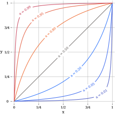
(a) $y=\operatorname{B}(x,a$)

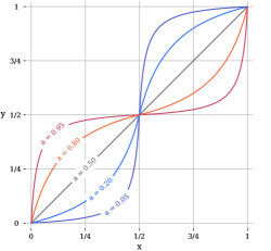
(b) $y=\operatorname{G}(x,a$)

Figure 1: Visualizations of Schlick’s bias and gain functions for different values of $a$.

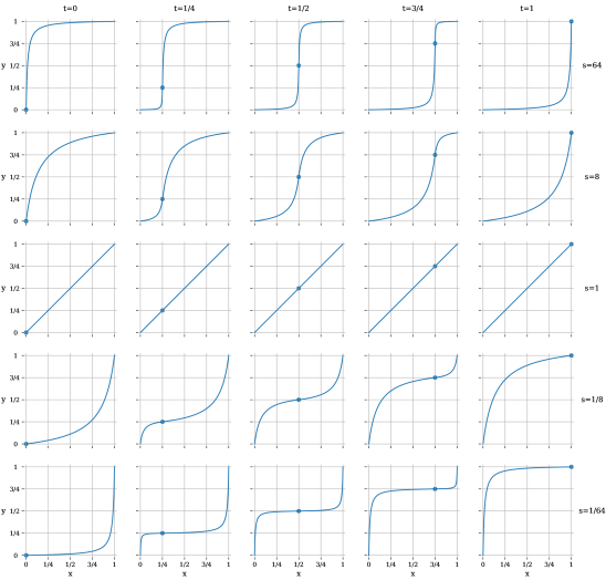
Figure 2: A “small multiples” visualization of $y=\operatorname{C}(x,s,t)$ for different values of $s$ (rows) and of $t$ (columns). A knot indicates where $x=t$. When $t$ is $0$ or $1$ (first column, last column) our generalization reproduces Schlick’s bias, and when $t$ is $\nicefrac{{1}}{{2}}$ (middle column) it reproduces Schlick’s gain.

References

- [1] Kenneth Perlin and Eric M Hoffert. Hypertexture. SIGGRAPH, 1989.
- [2] Christophe Schlick. Fast alternatives to perlin’s bias and gain functions. Graphics Gems, 4, 1994.