Effects of Parameter Norm Growth During Transformer Training:
Inductive Bias from Gradient Descent

Abstract

The capacity of neural networks like the widely adopted transformer is known to be very high. Evidence is emerging that they learn successfully due to inductive bias in the training routine, typically a variant of gradient descent (GD). To better understand this bias, we study the tendency for transformer parameters to grow in magnitude ($\ell_{2}$ norm) during training, and its implications for the emergent representations within self attention layers. Empirically, we document norm growth in the training of transformer language models, including T5 during its pretraining. As the parameters grow in magnitude, we prove that the network approximates a discretized network with saturated activation functions. Such “saturated” networks are known to have a reduced capacity compared to the full network family that can be described in terms of formal languages and automata. Our results suggest saturation is a new characterization of an inductive bias implicit in GD of particular interest for NLP. We leverage the emergent discrete structure in a saturated transformer to analyze the role of different attention heads, finding that some focus locally on a small number of positions, while other heads compute global averages, allowing counting. We believe understanding the interplay between these two capabilities may shed further light on the structure of computation within large transformers.

1 Introduction

Transformer-based models (Vaswani et al., 2017) like BERT (Devlin et al., 2019), XLNet (Yang et al., 2019), RoBERTa (Liu et al., 2019), and T5 (Raffel et al., 2019) have pushed the state of the art on an impressive array of NLP tasks. Overparameterized transformers are known to be universal approximators (Yun et al., 2020), suggesting their generalization performance ought to rely on useful biases or constraints imposed by the learning algorithm. Despite various attempts to study these biases in transformers (Rogers et al., 2020; Lovering et al., 2021), it remains an interesting open question what they are, or even how to characterize them in a way relevant to the domain of language.

In this work, we take the perspective that thoroughly understanding the dynamics of gradient descent (GD) might clarify the linguistic biases of transformers, and the types of representations they acquire. We start by making a potentially surprising empirical observation (§ 3): the parameter $\ell_{2}$ norm grows proportional to $\sqrt{t}$ (where $t$ is the timestep) during the training of T5 (Raffel et al., 2019) and other transformers. We refer to the phenomenon of growing parameter norm during training as norm growth. Previous work has analyzed norm growth in simplified classes of feedforward networks (Li and Arora, 2019; Ji and Telgarsky, 2020), but, to our knowledge, it has not been thoroughly demonstrated or studied in the more complicated and practical setting of transformers.

Our main contribution is analyzing the effect of norm growth on the representations within the transformer (§ 4), which control the network’s grammatical generalization. With some light assumptions, we prove that any network where the parameter norm diverges during training approaches a saturated network (Merrill et al., 2020): a restricted network variant whose discretized representations are understandable in terms of formal languages and automata. Empirically, we find that internal representations of pretrained transformers approximate their saturated counterparts, but for randomly initialized transformers, they do not. This suggests that the norm growth implicit in training guides transformers to approximate saturated networks, justifying studying the latter (Merrill, 2019) as a way to analyze the linguistic biases of NLP architectures and the structure of their representations.

Past work (Merrill, 2019; Bhattamishra et al., 2020) reveals that saturation permits two useful types of attention heads within a transformer: one that locally targets a small number of positions, and one that attends uniformly over the full sequence, enabling an “average” operation. Empirically, we find that both of these head types emerge in trained transformer language models. These capabilities reveal how the transformer can process various formal languages, and could also suggest how it might represent the structure of natural language. Combined, our theoretical and empirical results shed light on the linguistic inductive biases imbued in the transformer architecture by GD, and could serve as a tool to analyze transformers, visualize them, and improve their performance.

Finally, we discuss potential causes of norm growth in § 5. We prove transformers are approximately homogeneous Ji and Telgarsky (2020), a property that has been extensively studied in deep learning theory. With some simplifying assumptions, we then show how homogeneity might explain the $\sqrt{t}$ growth observed for T5.

2 Background and Related Work

2.1 GD and Deep Learning Theory

A simple case where deep learning theory has studied the generalization properties of GD is matrix factorization (Gunasekar et al., 2017; Arora et al., 2019; Razin and Cohen, 2020). It has been observed that deep matrix factorization leads to low-rank matrix solutions. Razin and Cohen (2020) argued theoretically that this bias of GD cannot be explained as an implicit regularizer minimizing some norm. Rather, they construct cases where all parameter norms diverge during GD.

Similar ideas have emerged in recent works studying feedforward networks. Analyzing biasless ReLU networks with cross-entropy loss, Poggio et al. (2019, 2020) show that the magnitude ($\ell_{2}$ norm) of the parameter vector continues to grow during GD, while its direction converges. Li and Arora (2019) present a similar argument for scale-invariant networks, meaning that scaling the parameters by a constant does not change the output. Studying homogeneous networks, Ji and Telgarsky (2020) show that the gradients become aligned as $t\to\infty$, meaning that their direction converges to the parameter direction. This means the norm will grow monotonically with $t$. The perspective developed by these works challenges the once conventional wisdom that the parameters converge to a finite local minimum during GD training. Rather, it suggests that GD follows a norm-increasing trajectory along which network behavior stabilizes. These analyses motivate investigation of this trajectory-driven perspective of training.

From a statistical perspective, work in this vein has considered the implications of these training dynamics for margin maximization (Poggio et al., 2019; Nacson et al., 2019; Lyu and Li, 2019). While these works vary in the networks they consider and their assumptions, they reach similar conclusions: GD follows trajectories diverging in the direction of a max-margin solution. As margin maximization produces a simple decision boundary, this property suggests better generalization than an arbitrary solution with low training loss. This point of view partially explains why growing norm is associated with better generalization performance.

2.2 NLP and Formal Language Theory

Norm growth has another interpretation for NLP models. Past work characterizes the capacity of infinite-norm networks in terms of formal languages and automata theory. Merrill (2019) and Merrill et al. (2020) propose saturation, a framework for theoretical analysis of the capacity of NLP architectures. A network is analyzed by assuming it saturates its nonlinearities, which means replacing functions like $\sigma$ and $\tanh$ with step functions. This is equivalent to the following definition:

Definition 1 (Saturation; Merrill et al., 2020).

Let $f(x;\theta)$ be a neural network with inputs $x$ and weights $\theta$. The saturated network $\textrm{s}f(x;\theta)$ is

$$\textrm{s}f(x;\theta)=\lim_{c\rightarrow\infty}f(x;c\theta),$$

where the limit exists, and undefined elsewhere.

Saturation reduces continuous neural networks to discrete computational models resembling automata or circuits, making some kinds of formal linguistic analysis easier. For many common architectures, the saturated capacity is known to be significantly weaker than the full capacity of the network with rational-valued weights (Merrill, 2019), which, classically, is Turing-complete for even simple RNNs (Siegelmann and Sontag, 1992).

For example, one can hand-construct an RNN or LSTM encoding a stack in its recurrent memory (Kirov and Frank, 2012). Stacks are useful for processing compositional structure in linguistic data (Chomsky, 1956), e.g., for semantic parsing. However, a saturated LSTM does not have enough memory to simulate a stack (Merrill, 2019). Rather, saturated LSTMs resemble classical counter machines (Merrill, 2019): automata limited in their ability to model hierarchical structure (Merrill, 2020). Experiments suggest that LSTMs trained on synthetic tasks learn to implement counter memory (Weiss et al., 2018; Suzgun et al., 2019a), and that they fail on tasks requiring stacks and other deeper models of structure (Suzgun et al., 2019b). Similarly, Shibata et al. (2020) found that LSTM language models trained on natural language data acquire saturated representations approximating counters.

Recent work extends saturation analysis to transformers (Merrill, 2019; Merrill et al., 2020). Saturated attention heads reduce to generalized hard attention, where the attention scores can tie. In the case of ties, the head output averages the positions with maximal scores. While their power is not fully understood, saturated transformers can implement a counting mechanism similarly to LSTMs (Merrill et al., 2020). In practice, Bhattamishra et al. (2020) show transformers can learn tasks requiring counting, and that they struggle when more complicated structural representations are required. Ebrahimi et al. (2020) find that attention patterns of certain heads can emulate bounded stacks, but that this ability falls off sharply for longer sequences. Thus, the abilities of trained LSTMs and transformers appear to be predicted by the classes of problems solvable by their saturated counterparts. Merrill et al. (2020) conjecture that the saturated capacity might represent a class of tasks implicitly learnable by GD, but it is unclear a priori why this should be the case. This work aims to put this conjecture on more solid theoretical footing: we argue that approximate saturation arises in transformers as a result of norm growth during training.

3 Norm Growth in Transformers

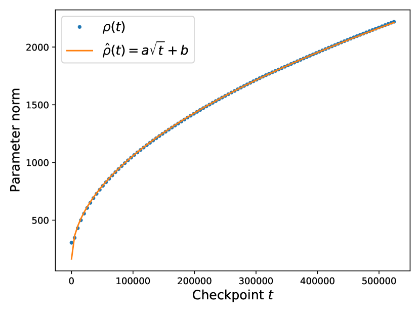
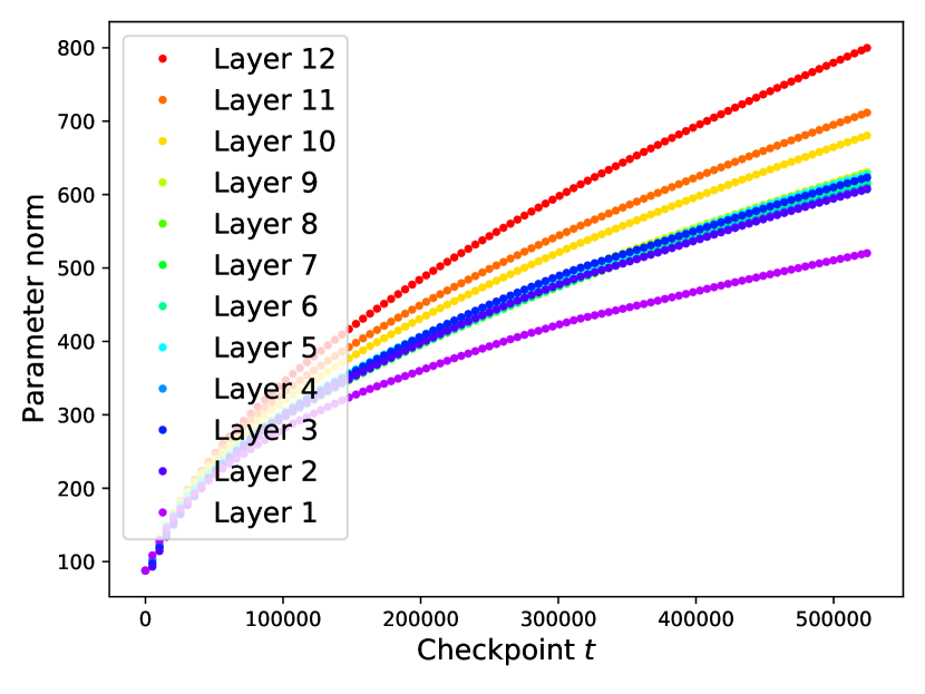
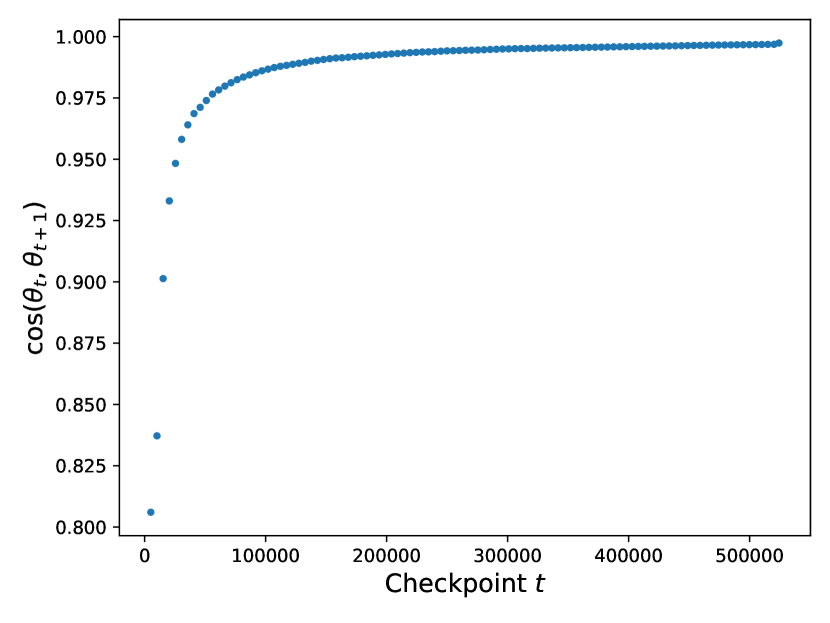
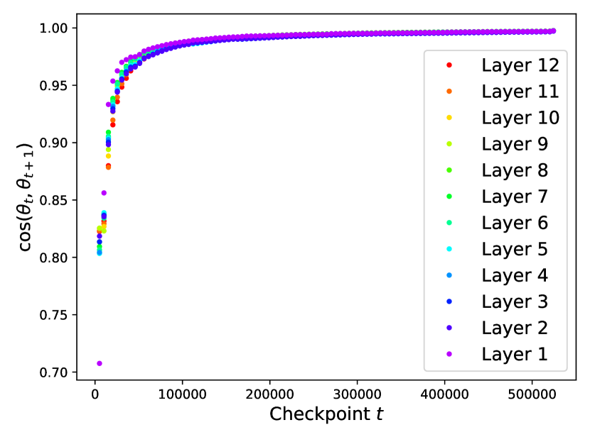
Figure 1: Top: Norm growth during T5 pretraining, with a coefficient $r^{2}=1.00$. The right is broken down by layer. Bottom: cosine similarity between subsequent parameter checkpoints.

We start with the observation that the parameter $\ell_{2}$ norm grows during training for practical transformer language models. We first consider the parameter norm of $104$ historical checkpoints from T5-base (Raffel et al., 2019) pretraining, a 220M parameter model, which was trained using the AdaFactor optimizer (Shazeer and Stern, 2018). Further details are in § A.

Fig. 1 shows that the T5 norm follows a $\sqrt{t}$ trend, where $t$ is time in training steps. The top right of Fig. 1 breaks down the growth trend by layer. Generally, the norm grows more quickly in later layers than in earlier ones, although always at a rate proportional to $\sqrt{t}$. Next, in the bottom row of Fig. 1, we plot the cosine similarity between each parameter checkpoint $\theta_{t+1}$ and its predecessor $\theta_{t}$. This rapidly approaches $1$, suggesting the “direction” of the parameters ($\theta_{t}/\norm{\theta_{t}}$) converges. The trend in directional convergence looks similar across layers.

We also train smaller transformer language models with 38M parameters on Wikitext-2 (Merity et al., 2016) and the Penn Treebank (PTB; Marcus et al., 1993). We consider two variants of the transformer: pre-norm and post-norm, which vary in the relative order of layer normalization and residual connections (cf. Xiong et al., 2020). Every model exhibits norm growth over training.

Combined, these results provide evidence that the parameter norm of transformers tends to grow over the course of training. In the remainder of this paper, we will discuss the implications of this phenomenon for the linguistic biases of transformers, and then discuss potential causes of the trend rooted in the optimization dynamics.

4 Effect of Norm Growth

§ 3 empirically documented that the parameter norm grows proportional to $\sqrt{t}$ during T5 pretraining. Now, we move to the main contribution of our paper: the implications of norm growth for understanding transformers’ linguistic inductive biases. In particular, Prop. 1 says uniform norm growth across the network guides GD towards saturated networks. Thus, saturation is not just a useful approximation for analyzing networks, but a state induced by training with enough time.

Proposition 1 (Informal).

Let $\theta_{t}\in\mathbb{R}^{n}$ be parameters at step $t$ for $f(x;\theta_{t})$. If every scalar parameter $\theta_{t}^{i}$ diverges at the same rate up to a constant, then $f$ converges pointwise to a saturated network.

The proof is in § B. Prop. 1 assumes not just norm growth, but uniform norm growth, meaning no parameter can asymptotically dominate any other. Notably, uniform growth implies directional convergence. Accepting uniform growth for a given training regimen, we expect transformers to converge to saturated networks with infinite training. Based on § 3, the T5 norm appears to grow $\propto\sqrt{t}$ uniformly across the network, suggesting the uniform growth condition is reasonable. As we will discuss later in § 5, we expect the growth trend to depend heavily on the learning rate schedule.

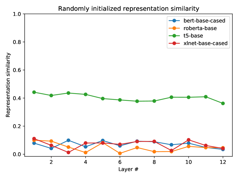
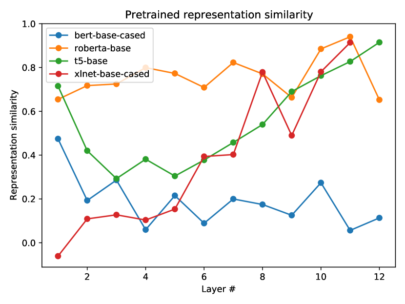
Figure 2: Cosine similarities of the unsaturated and saturated ($c=1{,}000$) transformer representations, by layer. We compare randomly initialized transformers (left) to pretrained ones (right).

4.1 Saturated Transformers

Having established that norm growth should lead to saturation, we now empirically measure the saturation levels in T5 and other transformer models.

Large transformers are highly saturated.

Since $\norm{\theta_{t}}$ empirically grows during training, we expect high cosine similarity between the representations in trained networks and saturated representations. We estimate this as the cosine similarity between $f(x;\theta)$ and $f(x;c\theta)$ for some large $c$ (in practice, $1{,}000$). We consider the “base” versions of pretrained BERT, RoBERTa, T5, and XLNet (pretrained on masked language modeling), and compute the mean saturation over $100$ input sentences from the Brown corpus (Francis and Kučera, 1989). To match standard practice, each sentence is truncated at $512$ word pieces. Fig. 2 plots the similarity for each layer of each model. We compare the pretrained transformers against a randomly initialized baseline. For every model type, the similarity is higher for the pretrained network than the randomly initialized network, which, except for T5, is ${\sim}0$. For T5 and XLNet, the similarity in the final layer is ${\geq}0.9$, whereas, for RoBERTa, the final similarity is $0.65$ (although $0.94$ in the penultimate layer). For T5 and XLNet, similarity is higher in later layers, which is potentially surprising, as one might expect error to compound with more layers. This may relate to the fact that the norm grows faster for later layers in T5. One question is why the similarity for BERT is lower than these models. As RoBERTa is architecturally similar to BERT besides longer training, we hypothesize that RoBERTa’s higher similarity is due to longer pretraining.

Small transformers reach full saturation.

Each of the transformers trained on Wikitext-2 and PTB reached a saturation level of $1.00$. It is unclear why these models saturate more fully than the pretrained ones, although it might be because they are smaller. For our LMs, the feedforward width ($512$) is less than for T5-base, while the encoder depth and width are the same. Other possible explanations include differences in the initialization scheme, optimizer, and training objective (masked vs. next-word modeling). See § A for full hyperparameters.

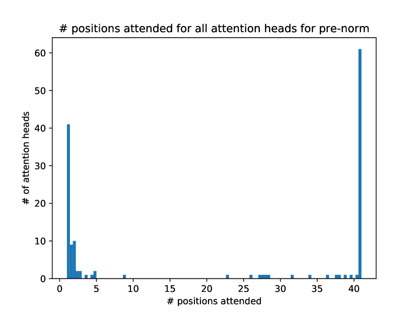
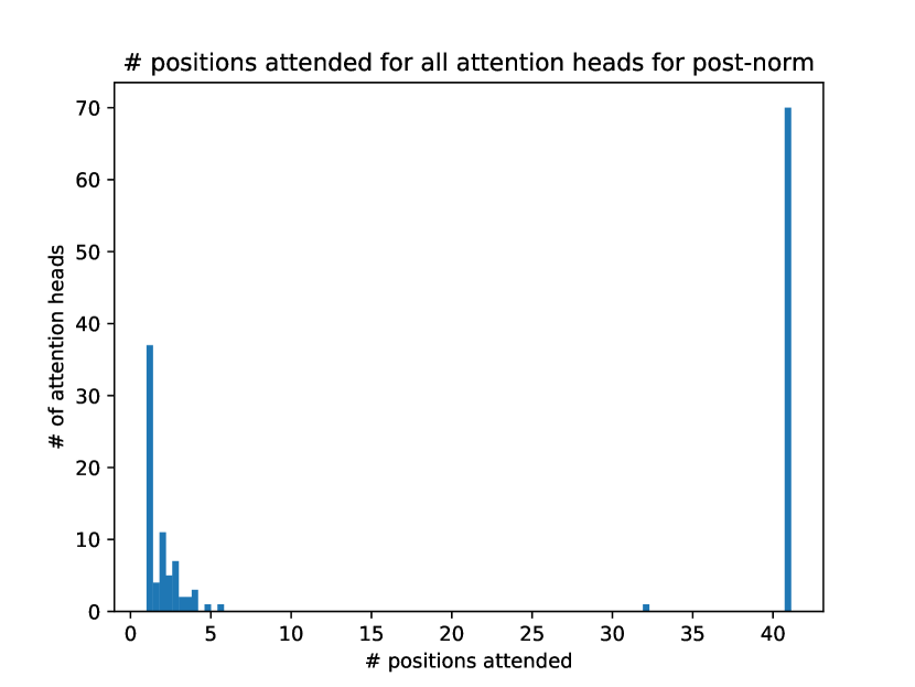
Figure 3: Distribution of the number of positions attended to for all heads in the PTB language models. The left plot is pre-norm, and the right is post-norm. Values are averaged over 200 sentences from the development set.

4.2 Power of Saturated Attention

We have shown that transformer training increases the parameter norm (§ 3), creating a bias towards saturation (§ 4.1). Now, we discuss the computational capabilities of saturated transformers, and empirically investigate how they manifest in pretrained transformers. What computation can saturated transformers perform? We review theoretical background about saturated attention, largely developed by Merrill (2019). Let $H$ (sequence length $n$ by model dimension $d$) be the input representation to a self attention layer. We assume a standard self attention mechanism with key, query, and value matrices $K,Q,V.$ Saturated attention resembles standard attention where softmax is constrained to a generalization of “argmax” (Merrill, 2019):

$$\textrm{s}\operatorname{\mathrm{attn}}(H;Q,K,V)=\arg\max(HQK^{\top}H^{\top})HV.$$

We define this vectorized $\arg\max(A)$ as

$$\mathcal{M}(A_{i}) =\{j\mid a_{ij}=\max_{k}a_{ik}\}$$

$$\arg\max(A_{i})_{j} =\begin{cases}1/\absolutevalue{\mathcal{M}(A_{i})}&\textrm{if}\;j\in\mathcal{M}(A_{i})\\ 0&\textrm{otherwise.}\end{cases}$$

Crucially, in the case of ties, $\arg\max(A)$ returns a uniform distribution over all tied positions. Saturated attention can retrieve the “maximum” value in a sequence according to some similarity matrix. It is also capable of restricted counting (Merrill et al., 2020). Formalizing these observations, we identify two useful computational operations that are reducible to saturated self attention: argmax and mean. Let $h_{i}$ represent the input representation at each time step $1\leq i\leq n$.

1. Argmax: Set $V=\mathrm{Id}$. Then the self attention mechanism computes a function recovering the element of $H$ that maximally resembles $h_{i}$ according to a quadratic form $M=KQ^{\top}$. If there is a tie for similarity, a uniform average of the maximal entries in $H$ is returned.

   $$\mathrm{argmax}(H;M)=\arg\max_{j}h_{i}Mh^{\top}_{j}.$$

2. Mean: Parameterize the head to attend uniformly everywhere. Then the head computes a function taking a uniform average of values:

   $$\mathrm{mean}(H;V)=\frac{1}{n}\sum_{j=1}^{n}Vh_{j}.$$ (1)

These constructions demonstrate some useful computational abilities of saturated transformers. Due to the summation in (1), the mean operation (or near variants of it) can be used to implement counting, which allows recognizing languages like $a^{n}b^{n}c^{n}$ (Merrill et al., 2020). Empirically, Bhattamishra et al. (2020) find trained networks can learn to recognize counter languages that rely on computing means, failing on more complicated languages like Dyck-2. Our findings partially justify why transformers can learn these languages: they lie within the capacity of saturated transformers.

4.3 Learned Attention Patterns

Recall that the small language models trained in § 4.1 reach $1.00$ saturation. It follows that we can convert them to saturated transformers (by multiplying $\theta$ by a large constant $c$) without significantly shifting the representations in cosine space. We will evaluate if the saturated attention heads manifest the argmax and mean constructions from § 4.2.

As discussed in § 4.2, saturated attention can parameterize both argmax and mean heads. An argmax head should attend to a small number of positions. A mean head, on the other hand, attends uniformly over the full sequence. Are both patterns acquired in practice by our models? We plot the distribution of the number of positions attended to by each head in the saturated PTB models in Fig. 3. The distribution is bimodal, with one mode at $1$, and the other around $41$, representing the mean sequence length of a $83$-length encoder with positional masking to prevent lookahead. The empirical mode around $1$ corresponds to heads that are argmax-like. The mode around $41$, on the other hand, corresponds to mean-like heads, since it implies uniform attention over the masked sequence. Thus, our analysis suggests that analogs of both types of attention heads theorized in § 4.2 are acquired in transformers in practice. In the pre-norm transformer, which performs substantially better, there are also a small number of heads lying between the two modes. We defer the investigation of the function of these heads to future work.

5 Explanation for Norm Growth

We have documented norm growth in T5 and other transformers (§ 3) and showed how it induces partial saturation in their representations (§ 4). This section points towards an understanding of why the parameter norm grows over the course of training, grounded in results about norm growth from deep learning theory. We do not analyze specific optimizers directly; instead, we analyze norm growth within simplified models of training dynamics taken from the literature. We then evaluate how these candidate dynamics models fit T5’s training.

5.1 Setup

Let $\delta_{t}\in\mathbb{R}^{n}$ denote the optimizer step at time $t$, i.e., $\delta_{t}=\theta_{t+1}-\theta_{t}$. We write $\eta_{t}$ for the learning rate at $t$. Let $\nabla_{\theta_{t}}L$ denote the gradient of the loss with respect to $\theta_{t}$. By GD, we refer to the update $\delta_{t}=-\eta_{t}\nabla_{\theta_{t}}L$. In contrast, we will use the term gradient flow to refer to its continuous relaxation, specified by an analogous differential equation:

$$\derivative{\theta_{t}}{t}=-\eta_{t}\nabla_{\theta_{t}}L.$$

5.2 Homogeneity

We will rely on properties of homogeneous networks, a class of architectures well-studied in deep learning theory (Ji and Telgarsky, 2020).

Definition 2 (Homogeneity).

A function $f(x;\theta)$ is $k$-homogeneous in $\theta$ iff, for all $c\geq 0$, $f(x;c\theta)=c^{k}f(x;\theta)$. We further say that $f$ is homogeneous iff there exists some $k$ such that $f$ is $k$-homogeneous.

Many common components of modern neural networks are homogeneous (Li and Arora, 2019). Furthermore, as various computations within a neural network preserve homogeneity (§ C), some full networks are also homogeneous. An example of a fully homogeneous neural network is a feedforward ReLU network without bias terms.

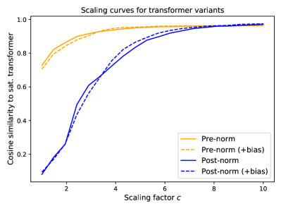
Figure 4: Approximate cosine similarity of $f(x;c\theta)$ to $\textrm{s}f(x;\theta)$ for randomly initialized transformers $f$. $\textrm{s}f(x;\theta)$ is approximated as in Fig. 2.

Why is homogeneity relevant for transformers? Transformers are not homogeneous, but they are almost homogeneous. We formalize this as:

Definition 3 (Approx. homogeneity).

A scalar function $f(x;\theta)$ is approximately $k$-homogeneous in $\theta$ iff there exist $d,\rho$ s.t., for $c\geq 1$ and $\norm{\theta}\geq\rho$,

$$\absolutevalue{f(x;c\theta)-c^{k}f(x;\theta)}\leq\exp(-d\norm{\theta}).$$

In other words, as $\norm{\theta}$ grows, $f$ approximates a homogeneous function with exponentially vanishing error. In § D, we prove transformer encoders without biases are approximately $1$-homogeneous. In Fig. 4, we compare the cosine similarity of transformers with and without biases to their saturated variants, as a function of a constant $c$ scaling their weights. An approximately homogeneous function rapidly approach $1.0$ as $c$ increases. We find similar curves for transformers with and without biases, suggesting biasless transformers are similarly homogeneous to transformers with biases.

Since multiplying two homogeneous functions adds their homogeneity, a transformer encoder followed by a linear classifier is approximately $2$-homogeneous. A key property of homogeneous functions is Euler’s Homogeneity Theorem: the derivative of a $k$-homogeneous function is $(k-1)$-homogeneous. Thus, we will assume the gradients of the linear classifier output are roughly $1$-homogeneous, which under simple GD implies:

Assumption 1.

Let $\theta_{t}$ include all encoder and classifier parameters. Let $\mathchoice{\mathrel{\vbox{ \offinterlineskip\halign{\hfil$#$\cr\displaystyle\propto\cr\kern 2.0pt\cr\displaystyle\sim\cr\kern-2.0pt\cr}}}}{\mathrel{\vbox{ \offinterlineskip\halign{\hfil$#$\cr\textstyle\propto\cr\kern 2.0pt\cr\textstyle\sim\cr\kern-2.0pt\cr}}}}{\mathrel{\vbox{ \offinterlineskip\halign{\hfil$#$\cr\scriptstyle\propto\cr\kern 2.0pt\cr\scriptstyle\sim\cr\kern-2.0pt\cr}}}}{\mathrel{\vbox{ \offinterlineskip\halign{\hfil$#$\cr\scriptscriptstyle\propto\cr\kern 2.0pt\cr\scriptscriptstyle\sim\cr\kern-2.0pt\cr}}}}$ mean “approximately proportional to”. For large enough $t$ during transformer training, $\norm{\delta_{t}}\mathchoice{\mathrel{\vbox{ \offinterlineskip\halign{\hfil$#$\cr\displaystyle\propto\cr\kern 2.0pt\cr\displaystyle\sim\cr\kern-2.0pt\cr}}}}{\mathrel{\vbox{ \offinterlineskip\halign{\hfil$#$\cr\textstyle\propto\cr\kern 2.0pt\cr\textstyle\sim\cr\kern-2.0pt\cr}}}}{\mathrel{\vbox{ \offinterlineskip\halign{\hfil$#$\cr\scriptstyle\propto\cr\kern 2.0pt\cr\scriptstyle\sim\cr\kern-2.0pt\cr}}}}{\mathrel{\vbox{ \offinterlineskip\halign{\hfil$#$\cr\scriptscriptstyle\propto\cr\kern 2.0pt\cr\scriptscriptstyle\sim\cr\kern-2.0pt\cr}}}}\eta_{t}\norm{\theta_{t}}$.

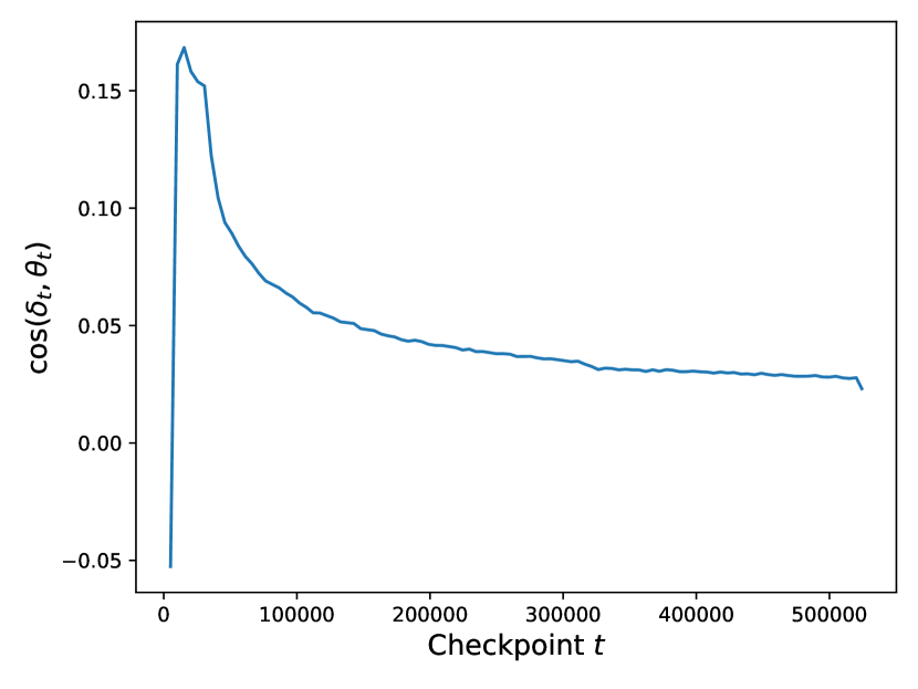
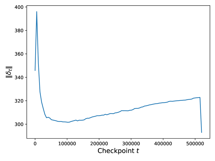
Figure 5: Alignment (cosine similarity of $\delta_{t}$ and $\theta_{t}$) and step size ($\norm{\delta_{t}}$) over training.

5.3 Aligned Dynamics

We now consider the first candidate dynamics model: aligned dynamics (Ji and Telgarsky, 2020). Analyzing homogeneous networks with an exponential binary classification loss and gradient flow, Ji and Telgarsky (2020) show that the parameters converge in direction, and that the gradients become aligned, meaning that $\theta_{t}^{\top}\cdot\delta_{t}\to\norm{\theta_{t}}\norm{\delta_{t}}$. While it is unclear whether transformers will follow aligned dynamics, we entertain this as one hypothesis. Under Ass. 1, alignment implies

$$\norm{\theta_{t}} \approx\sum_{i=0}^{t}\norm{\delta_{i}}\mathchoice{\mathrel{\vbox{ \offinterlineskip\halign{\hfil$#$\cr\displaystyle\propto\cr\kern 2.0pt\cr\displaystyle\sim\cr\kern-2.0pt\cr}}}}{\mathrel{\vbox{ \offinterlineskip\halign{\hfil$#$\cr\textstyle\propto\cr\kern 2.0pt\cr\textstyle\sim\cr\kern-2.0pt\cr}}}}{\mathrel{\vbox{ \offinterlineskip\halign{\hfil$#$\cr\scriptstyle\propto\cr\kern 2.0pt\cr\scriptstyle\sim\cr\kern-2.0pt\cr}}}}{\mathrel{\vbox{ \offinterlineskip\halign{\hfil$#$\cr\scriptscriptstyle\propto\cr\kern 2.0pt\cr\scriptscriptstyle\sim\cr\kern-2.0pt\cr}}}}\int\eta_{t}\norm{\theta_{t}}\mathrm{d}t.$$

With the $\eta_{t}=1/\sqrt{t}$ schedule used by T5 (Raffel et al., 2019), $\norm{\theta_{t}}\mathchoice{\mathrel{\vbox{ \offinterlineskip\halign{\hfil$#$\cr\displaystyle\propto\cr\kern 2.0pt\cr\displaystyle\sim\cr\kern-2.0pt\cr}}}}{\mathrel{\vbox{ \offinterlineskip\halign{\hfil$#$\cr\textstyle\propto\cr\kern 2.0pt\cr\textstyle\sim\cr\kern-2.0pt\cr}}}}{\mathrel{\vbox{ \offinterlineskip\halign{\hfil$#$\cr\scriptstyle\propto\cr\kern 2.0pt\cr\scriptstyle\sim\cr\kern-2.0pt\cr}}}}{\mathrel{\vbox{ \offinterlineskip\halign{\hfil$#$\cr\scriptscriptstyle\propto\cr\kern 2.0pt\cr\scriptscriptstyle\sim\cr\kern-2.0pt\cr}}}}\exp(\sqrt{t})$ (see § E.1). This is asymptotically faster than the observed $\sqrt{t}$ growth, suggesting an alternate dynamics might be at play.

5.4 Misaligned Dynamics

Our second candidate model of training is misaligned dynamics, which follows largely from Li and Arora (2019). This can be derived by assuming the gradients are misaligned (i.e., $\theta_{t}^{\top}\cdot\delta_{t}=0$), which hold for scale-invariant networks (Li and Arora, 2019) and in expectation for random normal gradients. Misalignment implies (derived in § E.2):

$$\norm{\theta_{t}}^{2}\mathchoice{\mathrel{\vbox{ \offinterlineskip\halign{\hfil$#$\cr\displaystyle\propto\cr\kern 2.0pt\cr\displaystyle\sim\cr\kern-2.0pt\cr}}}}{\mathrel{\vbox{ \offinterlineskip\halign{\hfil$#$\cr\textstyle\propto\cr\kern 2.0pt\cr\textstyle\sim\cr\kern-2.0pt\cr}}}}{\mathrel{\vbox{ \offinterlineskip\halign{\hfil$#$\cr\scriptstyle\propto\cr\kern 2.0pt\cr\scriptstyle\sim\cr\kern-2.0pt\cr}}}}{\mathrel{\vbox{ \offinterlineskip\halign{\hfil$#$\cr\scriptscriptstyle\propto\cr\kern 2.0pt\cr\scriptscriptstyle\sim\cr\kern-2.0pt\cr}}}}\sum_{i=0}^{t}\norm{\delta_{i}}^{2}.$$ (2)

We show in § E.2 that, with the T5 learning rate ($\eta_{t}=1/\sqrt{t}$), (2) reduces to $\norm{\theta_{t}}\mathchoice{\mathrel{\vbox{ \offinterlineskip\halign{\hfil$#$\cr\displaystyle\propto\cr\kern 2.0pt\cr\displaystyle\sim\cr\kern-2.0pt\cr}}}}{\mathrel{\vbox{ \offinterlineskip\halign{\hfil$#$\cr\textstyle\propto\cr\kern 2.0pt\cr\textstyle\sim\cr\kern-2.0pt\cr}}}}{\mathrel{\vbox{ \offinterlineskip\halign{\hfil$#$\cr\scriptstyle\propto\cr\kern 2.0pt\cr\scriptstyle\sim\cr\kern-2.0pt\cr}}}}{\mathrel{\vbox{ \offinterlineskip\halign{\hfil$#$\cr\scriptscriptstyle\propto\cr\kern 2.0pt\cr\scriptscriptstyle\sim\cr\kern-2.0pt\cr}}}}\sqrt{t}$, as observed empirically for T5. We now further test whether misaligned dynamics are a good fit for T5.

5.5 Evaluation

We measure the gradient alignment over the course of training T5. Our alignment metric is the cosine similarity of $\delta_{t}$ to $\theta_{t}$. As shown on the left of Fig. 5, the alignment initially rapidly increases to ${\sim}0.15$, and then decays to near $0$. This supports the hypothesis that the T5 dynamics are misaligned, since the similarity is never high, and may be approaching $0$.

On the right of Fig. 5, we plot step size over training in order to evaluate the validity of Ass. 1. At the beginning of training, a chaotic step size seems reasonable, as it is hard to predict the dynamics before approximate homogeneity takes hold. For large $t$, Ass. 1 combined with the T5 learning rate schedule predicts step size should be roughly constant. This is not exactly what we find: for large $t$, $\norm{\delta_{t}}$ grows gradually with $t$. However, the absolute change in step size is small: $<20$ across 220M parameters. Thus, we believe Ass. 1 is not unreasonable, though it would be interesting to understand what properties of the optimizer can explain the slight growth in step size.

5.6 Weight Decay

One feature of practical training schemes not considered in this section is weight decay. When applied to standard GD, weight decay can be written $\delta_{t}=-\eta_{t}\nabla_{\theta_{t}}L-\lambda\theta_{t}$. Intuitively, it might hinder norm growth if $\lambda$ is large. In § F, we report preliminary experiments testing the effect of weight decay on norm growth. Indeed, if $\lambda$ is set too large, weight decay can prevent norm growth, but within the standard range of values for $\lambda$, we find norm growth even in the face of weight decay. However, it is possible these results may change if the optimizer or other hyperparameters are varied.

6 Conclusion

We empirically found that $\norm{\theta_{t}}$ grows $\propto\sqrt{t}$ during T5 pretraining—a fact that may be caused by the approximate homogeneity of the transformer architecture. We proved that norm growth induces saturation, and then showed empirically that T5 and other large transformers become approximately saturated through their pretraining. Examining highly saturated transformer language models, we found the attention heads largely split between two distinct behaviors that can be roughly interpreted as argmax and mean operations. While we lack a precise formal characterization of “semi-saturated” transformers, we conjecture their capacity resembles that of the saturated models. Thus, we believe further analyzing the capabilities of saturated attention may clarify the linguistic biases that emerge in transformers through training, and the mechanisms they use to represent linguistic structure.

Appendix A Experimental Details

We provide experimental details for the small language models that we trained. The models were trained for 5 epochs, and the best performing model was selected based on development loss. Reported metrics were then measured on the held-out test set. We used our own implementation of the standard pre- and post-norm transformer architectures. We did not do any hyperparameter search, instead choosing the following hyperparameters:

• Batch size of $16$

• Model dimension of $768$

• Feedforward hidden dimension of $512$

• $12$ heads per layer

• $12$ layers

• AdamW optimizer with default PyTorch hyperparameters

• 0 probability of dropout

• Default PyTorch initialization

Tokenization

For Wikitext-2, $3$ tokens in the whole test dataset were unattested in the training set (due to capitalization). To make our model compatible with unseen tokens, we replaced these tokens with <unk>, the same class that appeared for low frequency words at training time, when evaluating the final text perplexity. Due to the small number of tokens that were affected, the impact of this change should be negligible.

Compute

We estimate the experiments in this paper took several hundred GPU hours on NVIDIA A100 GPUs over the course of almost two years of on-and-off research time.

T5

We used the historical checkpoints of bsl-0, one of five T5-base models that was trained for the original paper (Raffel et al., 2019).

Measuring Norms

As a systematic choice, all measurements of parameter norm include only encoder parameters that are not scalars. We advise other researchers to follow the practice of excluding embedding parameters, as embedding parameters that are infrequently updated may obscure general trends in the network parameters.

Appendix B Norm Growth and Saturation

Proposition 2 (Formal version of Prop. 1).

Let $\theta_{t}\in\mathbb{R}^{n}$ be the parameter vector at train step $t$ for a network $f(x;\theta_{t})$. Assume that, as $t\to\infty$, there exists a scalar sequence $c(t)\to\infty$ and fixed vector $\theta^{\prime}\in(\mathbb{R}\setminus\{0\})^{n}$ such that, for all $t$, $\theta_{t}\to\theta^{\prime}\cdot c(t)$. Then $f$ converges pointwise to a saturated network in function space.

Proof.

$$\lim_{t\to\infty}f(x;\theta_{t})=\lim_{t\to\infty}f(x;\theta^{\prime}\cdot c(t)).$$

Now, since $c(t)\to\infty$ and $\theta^{\prime}\cdot c(t)$ contains no indeterminate elements, we can simplify this to

$$\lim_{c\to\infty}f(x;c\theta^{\prime})=\textrm{s}f(x;\theta^{\prime}).$$

∎

Appendix C Approximate Homogeneity

In this section, we will further develop the notion of approximate homogeneity. We will prove that is consistent. In other words, every function can have at most one degree $k$ of approximate homogeneity. Next, we will show that the useful closure properties applying to full homogeneity also apply to partial homogeneity.

Component	$k$ Input	$k$ Output
Linear	$k$	$k+1$
Bias	$1$	$1$
Affine	$0$	$1$
LayerNorm	$k$	$0$
LayerNorm + Affine	$k$	$1$
ReLU	$k$	$k$
Sum	$(k,k)$	$k$
Product	$(k_{1},k_{2})$	$k_{1}+k_{2}$

Table 1: Effects of network components on homogeneity shown by Li and Arora (2019). We write the “$k$ Output” homogeneity as a function of the “$k$ Input” homogeneity. These facts can be applied recursively to compute the homogeneity of a network. We will show that the same facts hold for approximate homogeneity.

If $f(\theta)$ is approximately $k$-homogeneous (cf. Def. 3), then $f(c\theta)=c^{k}f(\theta)+\epsilon$ for some error vector $\epsilon$ where, for each $i$, $\absolutevalue{\epsilon_{i}}\leq\exp(-d\norm{\theta}))$, for all $c$ and large enough $\norm{\theta}$. We use this $\epsilon$ notation throughout this section.

C.1 Consistency

We first prove that approximate homogeneity is consistent: in other words, if a function is both approximately $k_{1}$ and $k_{2}$-homogeneous, then $k_{1}=k_{2}$. This is an important property for establishing approximate homogeneity as a meaningful notion.

Lemma 1.

Let $k_{1},k_{2}\in\mathbb{N}$. Assume that $f$ is both approximately $k_{1}$ and $k_{2}$-homogeneous. Then $k_{1}=k_{2}$.

Proof.

If $f$ is both approximately $k_{1}$ and $k_{2}$-homogeneous, then we have vanishing terms $\epsilon_{1}$ and $\epsilon_{2}$ such that, for all $c$,

$$f(c\theta) =c^{k_{1}}f(\theta)+\epsilon_{1}$$

$$f(c\theta) =c^{k_{2}}f(\theta)+\epsilon_{2}.$$

Subtracting both sides yields

$$0 =(c^{k_{1}}-c^{k_{2}})f(\theta)+\epsilon_{1}-\epsilon_{2}$$

$$\therefore\absolutevalue{c^{k_{1}}-c^{k_{2}}} =\frac{\absolutevalue{\epsilon_{1}-\epsilon_{2}}}{f(\theta)}.$$

The right-hand side vanishes exponentially in $\norm{\theta}$ for all $c$, whereas the left-hand side grows with $c$ unless $k_{1}=k_{2}$. Thus, to satisfy this equation for all $c$, it must be the case that $k_{1}=k_{2}$. ∎

C.2 Closure Properties

We now prove that effects of various functions on homogeneity explored by Li and Arora (2019) also translate to approximate homogeneity.

Lemma 2.

$\operatorname{\mathrm{ReLU}}$ preserves approximate $k$-homogeneity, i.e., let $f:\mathbb{R}^{n}\rightarrow\mathbb{R}$ be approximately $k$-homogeneous. Then $\operatorname{\mathrm{ReLU}}\circ f$ is approximately $k$-homogeneous.

Proof.

$$\operatorname{\mathrm{ReLU}}\big{(}f(c\theta)\big{)} =\operatorname{\mathrm{ReLU}}\big{(}c^{k}f(\theta)+\epsilon\big{)}$$

$$\leq\operatorname{\mathrm{ReLU}}\big{(}c^{k}f(\theta)\big{)}+\absolutevalue{\epsilon}.$$

Therefore,

$$\absolutevalue{\operatorname{\mathrm{ReLU}}\big{(}f(c\theta)\big{)}-\operatorname{\mathrm{ReLU}}\big{(}c^{k}f(\theta)\big{)}}\leq\absolutevalue{\epsilon}.$$

Set $\epsilon^{\prime}=\absolutevalue{\epsilon}$, showing $\operatorname{\mathrm{ReLU}}\big{(}f(\theta)\big{)}$ is approximately $k$-homogeneous. ∎

Lemma 3.

Let $f,g$ be vector-valued functions of $\theta$. If $f$ and $g$ are approximately $k$-homogeneous, then $f+g$ is approximately $k$-homogeneous.

Proof.

$$f(c\theta)+g(c\theta) =c^{k}f(\theta)+\epsilon_{f}+c^{k}g(\theta)+\epsilon_{g}$$

$$=c^{k}f(\theta)+c^{k}g(\theta)+\epsilon^{\prime},$$

where $\epsilon^{\prime}=\epsilon_{f}+\epsilon_{g}$. Thus,

$$\absolutevalue{f(c\theta)+g(c\theta)-c^{k}\big{(}f(\theta)+g(\theta)\big{)}}\leq\epsilon^{\prime}.$$

∎

Lemma 4.

Let $f,g$ be vector-valued functions of $\theta$. If $f$ and $g$ are approximately $k_{f}$ and $k_{g}$-homogeneous, then $f\cdot g$ is approximately $(k_{f}+k_{g})$-homogeneous.

Proof.

$$f(c\theta)\cdot g(c\theta) =\big{(}c^{k}f(\theta)+\epsilon_{f}\big{)}\cdot\big{(}c^{k}g(\theta)+\epsilon_{g}\big{)}$$

$$=c^{k_{f}+k_{g}}f(\theta)g(\theta)+c^{k_{f}}f(\theta)\epsilon_{g}$$

$$\quad+c^{k_{g}}g(\theta)\epsilon_{f}+\epsilon_{f}\epsilon_{g}.$$

We now rewrite the term $c^{k_{f}}f(\theta)\epsilon_{g}$ as

$$\frac{\theta g(x;\hat{\theta})}{\exp(-d\norm{\theta})}\leq\exp(-d^{\prime}\norm{\theta}).$$

Now, set $\epsilon^{\prime}=\min(\exp(-d\norm{\theta}),\epsilon_{f}\epsilon_{g})$.

$$\absolutevalue{f(c\theta)g(c\theta)-c^{k_{f}+k_{g}}f(\theta)g(\theta)}\leq\epsilon^{\prime}.$$

∎

The analogous results for linear transformation, bias, and affine transformation directly follow from the results for sum and product in Lem. 3 and Lem. 4.

Finally, we show that layer norm converts a homogeneous function to approximately scale-invariant function. In order to be numerically stable, practical implementations of layer norm utilize a small tolerance term so that the denominator is never zero. We omit this practical detail from our analysis, instead defining the layer norm $\operatorname{\mathrm{LN}}(x)$ for $x\in\mathbb{R}^{n}$ according to

$$\mu(x) =\frac{1}{n}\sum_{i=1}^{n}x_{i}$$

$$\operatorname{\mathrm{LN}}(x)_{i} =\frac{x_{i}-\mu(x)}{\norm{x-\mu(x)}}.$$

Lemma 5.

Let $f$ be approximately $k$-homogeneous for some $k$. Then, $\operatorname{\mathrm{LN}}(f)$ is approximately $0$-homogeneous.

Proof.

Since addition preserves approximate $k$-homogeneity, mean (and difference to mean), preserve approximate $k$-homogeneity. Letting $C=c^{k}$, we can write

$$f(c\theta)-\mu(f(c\theta))=C\big{(}f(\theta)-\mu(f(\theta))\big{)}+\epsilon.$$

We now apply this to the definition of layer norm to get

$$\operatorname{\mathrm{LN}}(f(c\theta))_{i} =\frac{f(c\theta)_{i}-\mu(f(c\theta))}{\norm{f(c\theta)-\mu(f(c\theta))}}$$

$$=\frac{C\big{(}f(\theta)_{i}-\mu(f(\theta))\big{)}+\epsilon_{i}}{C\norm{f(\theta)-\mu(f(\theta))}+\epsilon}.$$

We show that the difference between this and the unscaled layer norm goes to zero. To simplify notation, we now write $f=f(\theta)$, $\mu=\mu(f(\theta))$, and $\epsilon=\epsilon$ in the left-hand side below:

$$\absolutevalue{\operatorname{\mathrm{LN}}(f(c\theta))_{i}-\operatorname{\mathrm{LN}}(f(\theta)_{i})}$$

$$=\absolutevalue{\frac{C\big{(}f_{i}-\mu\big{)}+\epsilon_{i}}{C\norm{f-\mu}+\epsilon}-\frac{f_{i}-\mu}{\norm{f-\mu}}}$$

$$=\absolutevalue{\frac{\epsilon_{i}\norm{f-\mu}-\epsilon(f_{i}-\mu)}{C\norm{f-\mu}^{2}+\epsilon\norm{f-\mu}}}$$

$$=\absolutevalue{\frac{\epsilon_{i}-\epsilon v}{C\norm{f-\mu}+\epsilon}}$$

$$\leq\absolutevalue{\frac{\epsilon_{i}-\epsilon v}{\epsilon}}.$$

for some $v\in\mathbb{R}^{n}$ which does not grow with $\norm{\theta}$. Thus, setting $\epsilon^{\prime}$ to this final quantity satisfies the definition of approximate $0$-homogeneity, i.e. approximate scale invariance. ∎

C.3 Saturating Activation Functions

We show that the exponentially saturation activation functions $\sigma$, $\operatorname{\mathrm{softmax}}$, and $\tanh$ are approximately scale-invariant in $x$, i.e. scaling $x$ has an exponentially diminishing effect on the output. We start by analyzing the simpler sigmoid, and then show that the same result holds for softmax. For completeness, we then present a proof for $\tanh$. We use $\Theta$ (not $\theta$) in the standard sense of asymptotic notation.

Lemma 6.

The scaling error for $\sigma$ vanishes exponentially in the preactivation magnitude, i.e. for all $c\geq 1$,

$$\absolutevalue{\sigma(cx)-\sigma(x)}\leq\Theta(\exp(-\absolutevalue{x})).$$

Proof.

Assume without loss of generality that $x\neq 0$, as if this is the case, the error is $0$. When $x>0$, we have

$$\absolutevalue{\sigma(cx)-\sigma(x)} =\sigma(cx)-\sigma(x)$$

$$\leq 1-\sigma(\absolutevalue{x})$$

$$=\frac{1}{\exp(\absolutevalue{x})+1}$$

$$=\Theta(\exp(-\absolutevalue{x})).$$

When $x<0$, we have

$$\absolutevalue{\sigma(cx)-\sigma(x)} =\sigma(x)-\sigma(cx)$$

$$\leq 1-\sigma(\absolutevalue{x})+0$$

$$=\Theta(\exp(-\absolutevalue{x})).$$

∎

Lemma 7.

The elementwise scaling error for $\operatorname{\mathrm{softmax}}$ vanishes exponentially in the preactivation norm, i.e. for all $c\geq 1$, $x\in\mathbb{R}^{n}$ s.t. $1\leq i\leq n$,

$$\absolutevalue{\operatorname{\mathrm{softmax}}(cx)_{i}-\operatorname{\mathrm{softmax}}(x)_{i}}\leq\exp(-\Theta(\norm{x})).$$

Proof.

The proof closely follows that of Lem. 6, but is more involved. We consider two cases: $x_{i}=\max(x)$, and $x_{i}\neq\max(x)$.

Case 1

$x_{i}=\max(x)$.

$$\absolutevalue{\operatorname{\mathrm{softmax}}(cx)_{i}-\operatorname{\mathrm{softmax}}(x)_{i}}$$

$$=\operatorname{\mathrm{softmax}}(cx)_{i}-\operatorname{\mathrm{softmax}}(x)_{i}$$

$$\leq 1-\operatorname{\mathrm{softmax}}(x)_{i}$$

$$=1-\frac{\exp(x_{i})}{\sum_{j}\exp(x_{j})}$$

$$\leq 1-\frac{\exp(\max(x))}{\exp(\max(x))+(n-1)\exp(\min(x))}$$

$$=1-\frac{1}{1+(n-1)\exp(\min(x)-\max(x))}$$

$$=1-\frac{1}{1+\exp(\min(x)-\max(x)+d)},$$

for some $d\in\mathbb{R}$. As this has the form of $\sigma$,

$$\absolutevalue{\operatorname{\mathrm{softmax}}(cx)_{i}-\operatorname{\mathrm{softmax}}(x)_{i}}$$

$$=1-\sigma(\Theta(\norm{x}))=\exp(-\Theta(\norm{x})).$$

Case 2

$x_{i}\neq\max(x)$.

$$\absolutevalue{\operatorname{\mathrm{softmax}}(cx)_{i}-\operatorname{\mathrm{softmax}}(x)_{i}}$$

$$=\operatorname{\mathrm{softmax}}(x)_{i}-\operatorname{\mathrm{softmax}}(cx)_{i}$$

$$\leq 1-\max(\operatorname{\mathrm{softmax}}(x))-0$$

$$=1-\operatorname{\mathrm{softmax}}(\max(x)),$$

which is identical to case 1. ∎

Finally, for completeness, we show that $\tanh$ exhibits the same property. The proof is very similar to sigmoid, following closely from the definition

$$\tanh(x)=\frac{\exp(2x)-1}{\exp(2x)+1}.$$

Lemma 8.

The scaling error for $\tanh$ vanishes exponentially in the preactivation magnitude, i.e. for all $c\geq 1$,

$$\absolutevalue{\tanh(cx)-\tanh(x)}\leq\exp(-\Theta(\absolutevalue{x})).$$

Proof.

$$\absolutevalue{\tanh(cx)-\tanh(x)} \leq\absolutevalue{1-\tanh(x)}$$

$$=1-\tanh(\absolutevalue{x})$$

$$=1-\frac{\exp(2\absolutevalue{x})-1}{\exp(2\absolutevalue{x})+1}$$

$$=\frac{\exp(2\absolutevalue{x})+1-\exp(2\absolutevalue{x})+1}{\exp(2\absolutevalue{x})+1}$$

$$=\frac{2}{\exp(2\absolutevalue{x})+1}$$

$$=\exp(-\Theta(\absolutevalue{x})).$$

∎

Thus, applying these functions to a homogeneous input produces an output that is approximately scale-invariant in the parameters $\theta$. Thus, these functions act similarly to layer norm, which maps homogeneous input to scale-invariant output. But what happens if the input is approximately homogeneous, rather than strictly homogeneous? In this case, we show that the output is approximately scale-invariant assuming $\norm{\theta}$ is sufficiently large.

Proposition 3.

Let $f(x;\theta)$ be approximately $k$-homogeneous in $\theta$. Then the following functions are approximately scale-invariant in $\theta$:

$$g_{\sigma} =\sigma\circ f$$

$$g_{\operatorname{\mathrm{softmax}}} =\operatorname{\mathrm{softmax}}\circ f$$

$$g_{\tanh} =\tanh\circ f.$$

Proof.

If $f(x;\theta)$ is approximately $k$-homogeneous, then $f(x;c\theta)=c^{k}f(x;\theta)+\epsilon$ where $\norm{\epsilon}\leq\exp(-O(\norm{\theta}))$. Crucially, since $\epsilon$ vanishes for large norm, there is some $\rho$ where, for all $\theta$ such that $\rho<\norm{\theta}$:

$$\operatorname{\mathrm{sgn}}\big{(}c^{k}f(x;\theta)+\epsilon\big{)} =\operatorname{\mathrm{sgn}}\big{(}c^{k}f(x;\theta)\big{)}$$

$$\arg\max\big{(}c^{k}f(x;\theta)+\epsilon\big{)} =\arg\max\big{(}c^{k}f(x;\theta)\big{)}.$$

Therefore, for $\theta$ such that $\norm{\theta}>\rho$, the bounds used in Lem. 6, Lem. 7, and Lem. 8 hold for approximately homogeneous $f$. Thus, we can conclude that the output is approximately scale-invariant. ∎

Appendix D Transformers

We introduce the notation ${\sim}k$-homogeneous to mean approximately $k$-homogeneous. In this section, we show that the transformer encoder is ${\sim}1$-homogeneous. A transformer Vaswani et al. (2017) is made up of three main components: an embedding layer, self attention sublayers, and feed-forward sublayers. Since the embedding layer is just a matrix multiplication, it is a $1$-homogeneous function of the input. Assuming the self attention and feed-forward sublayers have no bias terms, we show that they approximate functions preserving approximate $1$-homogeneity. As the full network is an initial embedding layer followed by these sublayers, the final output is ${\sim}1$-homogeneous. In the main paper, we discuss the connection between homogeneity and norm growth.

We base our analysis on the HuggingFace implementation of BERT (Wolf et al., 2019). To aid analysis, we make some simplifying assumptions, which are discussed along with the definitions. We later show empirically that homogeneity for the unsimplified versions is similar.

D.1 Transformer Definition

The transformer encoder is a cascade of alternating multi-head self-attention sublayers and feedforward sublayers. Each multi-head self-attention sublayer can be further broken down as an aggregation of self-attention heads. Let $\operatorname{\mathrm{LN}}(\cdot)$ denote a layer norm followed by a learned affine transformation. Here we will consider the pre-norm transformer variant (Xiong et al., 2020), meaning that $\operatorname{\mathrm{LN}}$ comes before the residual connection wherever it appears. We will also assume that there are no biases, making all affine transformations into strict linear transformations.

Definition 4 (Self-attention head).

Given parameters $W^{k}$, $W^{q}$, $W^{v}$ and input $X\in\mathbb{R}^{Tn}$, we define a self-attention head $\operatorname{\mathrm{attn}}$ as

$$K =W^{k}X$$

$$Q =W^{q}X$$

$$V =W^{v}X$$

$$A =\operatorname{\mathrm{softmax}}(QK^{\top}/\sqrt{d_{k}})$$

$$H =AV,$$

where $H$ is the output tensor.

The multi-head self-attention sublayer computes several attention heads in parallel and aggregates them into a single sequence of vectors.

Definition 5 (Multi-head self-attention sublayer).

Let $X\in\mathbb{R}^{Tn}$ be the input. We now define the $k$-multi-head self-attention sublayer $\operatorname{\mathrm{MSA}}_{k}$. First, we compute $k$ self-attention heads in parallel to produce $H_{1},\cdots,H_{k}$. We then concatenate these along the feature axis to form $H$, and compute the sublayer output $Y$ as

$$\operatorname{\mathrm{MSA}}_{k}(X)=\operatorname{\mathrm{LN}}(WH)+X.$$

Finally, the linear sublayer is the other component of the transformer.

Definition 6 (Feedforward sublayer).

Let $X\in\mathbb{R}^{Tn}$ be the input. We compute the feedforward sublayer $\operatorname{\mathrm{FF}}$ according to

$$\operatorname{\mathrm{FF}}(X)=\operatorname{\mathrm{LN}}(W^{f}\operatorname{\mathrm{ReLU}}(W^{i}X))+X.$$

D.2 Results

Proposition 4.

If $X$ is ${\sim}1$-homogeneous in parameters $\theta$, then $\operatorname{\mathrm{attn}}(X;W^{k},W^{q},W^{v})$ is ${\sim}1$-homogeneous in the concatenation of $\theta,W^{k},W^{q},W^{v}$.

Proof.

Consider a self-attention layer receiving a ${\sim}1$-homogeneous input matrix $X\in\mathbb{R}^{Tn}$ where $T$ is the sequence length. Using the homogeneity rule for multiplication, $K,Q,V$ are each ${\sim}2$-homogeneous, as homogeneity is additive over multiplication. By the same argument, $QK^{\top}$ is ${\sim}4$-homogeneous. In Prop. 3, we show that if the input to softmax is approximately homogeneous, then the output is approximately scale-invariant. Thus, $A$ is approximately $0$-homogeneous. Then $AV$ is ${\sim}1$-homogeneous. ∎

We show that the multi-head component that aggregates multiple heads into a shared representation also preserves approximate $1$-homogeneity.

Proposition 5.

If $X$ is ${\sim}1$-homogeneous in parameters $\theta$, then $\operatorname{\mathrm{MSA}}$ is ${\sim}1$-homogeneous in the full parameters.

Proof.

Since $Wh$ is ${\sim}2$-homogeneous, $\operatorname{\mathrm{LN}}(WH)$ is ${\sim}1$-homogeneous. The input $X$ is also ${\sim}1$-homogeneous by assumption, meaning that the sum is also ${\sim}1$-homogeneous. ∎

Finally, we turn to analyzing the feedforward sublayer of the transformer.

Proposition 6.

If $X$ is ${\sim}1$-homogeneous, then $\operatorname{\mathrm{FF}}(X;W^{f},W^{i})$ is ${\sim}1$-homogeneous in the full parameters.

Proof.

Multiplying by each $W$ increases approximate homogeneity by $1$, and $\operatorname{\mathrm{ReLU}}$ preserves approximate homogeneity. So the input to $\operatorname{\mathrm{LN}}$ is ${\sim}3$-homogeneous. Thus, its output is ${\sim}1$-homogeneous, and adding $X$ preserves approximate $1$-homogeneity. ∎

Together, these results suggest that the pre-norm transformer output is ${\sim}1$-homogeneous, assuming its input is ${\sim}1$-homogeneous. This precondition for the input holds in the “base case” of standard embeddings. By induction, we can imagine the output of a biasless pre-norm transformer encoder of any depth to be ${\sim}1$-homogeneous.

Interestingly, the homogeneity arguments do not work out if we instead consider the post-norm transformer architecture (Xiong et al., 2020).

Appendix E Sum Derivation

E.1 Aligned Case

Assume that $\norm{\theta_{t}}\approx 0$. Then,

$$\norm{\theta_{t}} \mathchoice{\mathrel{\vbox{ \offinterlineskip\halign{\hfil$#$\cr\displaystyle\propto\cr\kern 2.0pt\cr\displaystyle\sim\cr\kern-2.0pt\cr}}}}{\mathrel{\vbox{ \offinterlineskip\halign{\hfil$#$\cr\textstyle\propto\cr\kern 2.0pt\cr\textstyle\sim\cr\kern-2.0pt\cr}}}}{\mathrel{\vbox{ \offinterlineskip\halign{\hfil$#$\cr\scriptstyle\propto\cr\kern 2.0pt\cr\scriptstyle\sim\cr\kern-2.0pt\cr}}}}{\mathrel{\vbox{ \offinterlineskip\halign{\hfil$#$\cr\scriptscriptstyle\propto\cr\kern 2.0pt\cr\scriptscriptstyle\sim\cr\kern-2.0pt\cr}}}}\int\eta_{t}\norm{\theta_{t}}\mathrm{d}t$$

$$\frac{\mathrm{d}}{\mathrm{d}t}\norm{\theta_{t}} \mathchoice{\mathrel{\vbox{ \offinterlineskip\halign{\hfil$#$\cr\displaystyle\propto\cr\kern 2.0pt\cr\displaystyle\sim\cr\kern-2.0pt\cr}}}}{\mathrel{\vbox{ \offinterlineskip\halign{\hfil$#$\cr\textstyle\propto\cr\kern 2.0pt\cr\textstyle\sim\cr\kern-2.0pt\cr}}}}{\mathrel{\vbox{ \offinterlineskip\halign{\hfil$#$\cr\scriptstyle\propto\cr\kern 2.0pt\cr\scriptstyle\sim\cr\kern-2.0pt\cr}}}}{\mathrel{\vbox{ \offinterlineskip\halign{\hfil$#$\cr\scriptscriptstyle\propto\cr\kern 2.0pt\cr\scriptscriptstyle\sim\cr\kern-2.0pt\cr}}}}\eta_{t}\norm{\theta_{t}}$$

$$\frac{\mathrm{d}\norm{\theta_{t}}}{\norm{\theta_{t}}} \mathchoice{\mathrel{\vbox{ \offinterlineskip\halign{\hfil$#$\cr\displaystyle\propto\cr\kern 2.0pt\cr\displaystyle\sim\cr\kern-2.0pt\cr}}}}{\mathrel{\vbox{ \offinterlineskip\halign{\hfil$#$\cr\textstyle\propto\cr\kern 2.0pt\cr\textstyle\sim\cr\kern-2.0pt\cr}}}}{\mathrel{\vbox{ \offinterlineskip\halign{\hfil$#$\cr\scriptstyle\propto\cr\kern 2.0pt\cr\scriptstyle\sim\cr\kern-2.0pt\cr}}}}{\mathrel{\vbox{ \offinterlineskip\halign{\hfil$#$\cr\scriptscriptstyle\propto\cr\kern 2.0pt\cr\scriptscriptstyle\sim\cr\kern-2.0pt\cr}}}}\eta_{t}\mathrm{d}t$$

$$\log\norm{\theta_{t}} \mathchoice{\mathrel{\vbox{ \offinterlineskip\halign{\hfil$#$\cr\displaystyle\propto\cr\kern 2.0pt\cr\displaystyle\sim\cr\kern-2.0pt\cr}}}}{\mathrel{\vbox{ \offinterlineskip\halign{\hfil$#$\cr\textstyle\propto\cr\kern 2.0pt\cr\textstyle\sim\cr\kern-2.0pt\cr}}}}{\mathrel{\vbox{ \offinterlineskip\halign{\hfil$#$\cr\scriptstyle\propto\cr\kern 2.0pt\cr\scriptstyle\sim\cr\kern-2.0pt\cr}}}}{\mathrel{\vbox{ \offinterlineskip\halign{\hfil$#$\cr\scriptscriptstyle\propto\cr\kern 2.0pt\cr\scriptscriptstyle\sim\cr\kern-2.0pt\cr}}}}\int\eta_{t}\mathrm{d}t$$

$$\norm{\theta_{t}} \mathchoice{\mathrel{\vbox{ \offinterlineskip\halign{\hfil$#$\cr\displaystyle\propto\cr\kern 2.0pt\cr\displaystyle\sim\cr\kern-2.0pt\cr}}}}{\mathrel{\vbox{ \offinterlineskip\halign{\hfil$#$\cr\textstyle\propto\cr\kern 2.0pt\cr\textstyle\sim\cr\kern-2.0pt\cr}}}}{\mathrel{\vbox{ \offinterlineskip\halign{\hfil$#$\cr\scriptstyle\propto\cr\kern 2.0pt\cr\scriptstyle\sim\cr\kern-2.0pt\cr}}}}{\mathrel{\vbox{ \offinterlineskip\halign{\hfil$#$\cr\scriptscriptstyle\propto\cr\kern 2.0pt\cr\scriptscriptstyle\sim\cr\kern-2.0pt\cr}}}}\exp\left(\int\eta_{t}\mathrm{d}t\right).$$

Plugging in $\eta_{t}=1/\sqrt{t}$, we get $\norm{\theta_{t}}\mathchoice{\mathrel{\vbox{ \offinterlineskip\halign{\hfil$#$\cr\displaystyle\propto\cr\kern 2.0pt\cr\displaystyle\sim\cr\kern-2.0pt\cr}}}}{\mathrel{\vbox{ \offinterlineskip\halign{\hfil$#$\cr\textstyle\propto\cr\kern 2.0pt\cr\textstyle\sim\cr\kern-2.0pt\cr}}}}{\mathrel{\vbox{ \offinterlineskip\halign{\hfil$#$\cr\scriptstyle\propto\cr\kern 2.0pt\cr\scriptstyle\sim\cr\kern-2.0pt\cr}}}}{\mathrel{\vbox{ \offinterlineskip\halign{\hfil$#$\cr\scriptscriptstyle\propto\cr\kern 2.0pt\cr\scriptscriptstyle\sim\cr\kern-2.0pt\cr}}}}\exp(\sqrt{t})$.

E.2 Misaligned Case

First, we derive the sum approximation for $\norm{\theta_{t}}$. We start with the fact that $\theta_{t+1}=\theta_{t}+\delta_{t}$ and misalignment, i.e., $\theta_{t}^{\top}\cdot\delta_{t}=0$.

$$\norm{\theta_{t+1}}^{2} =(\theta_{t}+\delta_{t})\cdot(\theta_{t}+\delta_{t})$$

$$=\norm{\theta_{t}}^{2}+\theta_{t}^{\top}\delta_{t}+\norm{\delta_{t}}^{2}$$

$$=\norm{\theta_{t}}^{2}+\norm{\delta_{t}}^{2}$$

$$=\norm{\theta_{0}}^{2}+\sum_{i=0}^{t}\norm{\delta_{i}}^{2}.$$

Taking the square root of both sides, $\norm{\theta_{t}}$ is roughly proportional to $\sum_{i=0}^{t}\norm{\delta_{i}}^{2}$.

Next, we show how to solve the integral, similarly to § E.1.

$$\norm{\theta_{t}}^{2} \mathchoice{\mathrel{\vbox{ \offinterlineskip\halign{\hfil$#$\cr\displaystyle\propto\cr\kern 2.0pt\cr\displaystyle\sim\cr\kern-2.0pt\cr}}}}{\mathrel{\vbox{ \offinterlineskip\halign{\hfil$#$\cr\textstyle\propto\cr\kern 2.0pt\cr\textstyle\sim\cr\kern-2.0pt\cr}}}}{\mathrel{\vbox{ \offinterlineskip\halign{\hfil$#$\cr\scriptstyle\propto\cr\kern 2.0pt\cr\scriptstyle\sim\cr\kern-2.0pt\cr}}}}{\mathrel{\vbox{ \offinterlineskip\halign{\hfil$#$\cr\scriptscriptstyle\propto\cr\kern 2.0pt\cr\scriptscriptstyle\sim\cr\kern-2.0pt\cr}}}}\int\norm{\delta_{t}}^{2}\mathrm{d}t$$

$$\norm{\theta_{t}}^{2} \mathchoice{\mathrel{\vbox{ \offinterlineskip\halign{\hfil$#$\cr\displaystyle\propto\cr\kern 2.0pt\cr\displaystyle\sim\cr\kern-2.0pt\cr}}}}{\mathrel{\vbox{ \offinterlineskip\halign{\hfil$#$\cr\textstyle\propto\cr\kern 2.0pt\cr\textstyle\sim\cr\kern-2.0pt\cr}}}}{\mathrel{\vbox{ \offinterlineskip\halign{\hfil$#$\cr\scriptstyle\propto\cr\kern 2.0pt\cr\scriptstyle\sim\cr\kern-2.0pt\cr}}}}{\mathrel{\vbox{ \offinterlineskip\halign{\hfil$#$\cr\scriptscriptstyle\propto\cr\kern 2.0pt\cr\scriptscriptstyle\sim\cr\kern-2.0pt\cr}}}}\int\eta_{t}^{2}\norm{\theta_{t}}^{2}\mathrm{d}t$$

$$\frac{\mathrm{d}}{\mathrm{d}t}\norm{\theta_{t}}^{2} \mathchoice{\mathrel{\vbox{ \offinterlineskip\halign{\hfil$#$\cr\displaystyle\propto\cr\kern 2.0pt\cr\displaystyle\sim\cr\kern-2.0pt\cr}}}}{\mathrel{\vbox{ \offinterlineskip\halign{\hfil$#$\cr\textstyle\propto\cr\kern 2.0pt\cr\textstyle\sim\cr\kern-2.0pt\cr}}}}{\mathrel{\vbox{ \offinterlineskip\halign{\hfil$#$\cr\scriptstyle\propto\cr\kern 2.0pt\cr\scriptstyle\sim\cr\kern-2.0pt\cr}}}}{\mathrel{\vbox{ \offinterlineskip\halign{\hfil$#$\cr\scriptscriptstyle\propto\cr\kern 2.0pt\cr\scriptscriptstyle\sim\cr\kern-2.0pt\cr}}}}\eta_{t}^{2}\norm{\theta_{t}}^{2}$$

$$\frac{\mathrm{d}\norm{\theta_{t}}^{2}}{\norm{\theta_{t}}^{2}} \mathchoice{\mathrel{\vbox{ \offinterlineskip\halign{\hfil$#$\cr\displaystyle\propto\cr\kern 2.0pt\cr\displaystyle\sim\cr\kern-2.0pt\cr}}}}{\mathrel{\vbox{ \offinterlineskip\halign{\hfil$#$\cr\textstyle\propto\cr\kern 2.0pt\cr\textstyle\sim\cr\kern-2.0pt\cr}}}}{\mathrel{\vbox{ \offinterlineskip\halign{\hfil$#$\cr\scriptstyle\propto\cr\kern 2.0pt\cr\scriptstyle\sim\cr\kern-2.0pt\cr}}}}{\mathrel{\vbox{ \offinterlineskip\halign{\hfil$#$\cr\scriptscriptstyle\propto\cr\kern 2.0pt\cr\scriptscriptstyle\sim\cr\kern-2.0pt\cr}}}}\eta_{t}^{2}\mathrm{d}t$$

$$\log\norm{\theta_{t}}^{2} \mathchoice{\mathrel{\vbox{ \offinterlineskip\halign{\hfil$#$\cr\displaystyle\propto\cr\kern 2.0pt\cr\displaystyle\sim\cr\kern-2.0pt\cr}}}}{\mathrel{\vbox{ \offinterlineskip\halign{\hfil$#$\cr\textstyle\propto\cr\kern 2.0pt\cr\textstyle\sim\cr\kern-2.0pt\cr}}}}{\mathrel{\vbox{ \offinterlineskip\halign{\hfil$#$\cr\scriptstyle\propto\cr\kern 2.0pt\cr\scriptstyle\sim\cr\kern-2.0pt\cr}}}}{\mathrel{\vbox{ \offinterlineskip\halign{\hfil$#$\cr\scriptscriptstyle\propto\cr\kern 2.0pt\cr\scriptscriptstyle\sim\cr\kern-2.0pt\cr}}}}\int\eta_{t}^{2}\mathrm{d}t.$$

Now, we plug in the $\eta_{t}=1/\sqrt{t}$ learning rate:

$$\log\norm{\theta_{t}}^{2} \mathchoice{\mathrel{\vbox{ \offinterlineskip\halign{\hfil$#$\cr\displaystyle\propto\cr\kern 2.0pt\cr\displaystyle\sim\cr\kern-2.0pt\cr}}}}{\mathrel{\vbox{ \offinterlineskip\halign{\hfil$#$\cr\textstyle\propto\cr\kern 2.0pt\cr\textstyle\sim\cr\kern-2.0pt\cr}}}}{\mathrel{\vbox{ \offinterlineskip\halign{\hfil$#$\cr\scriptstyle\propto\cr\kern 2.0pt\cr\scriptstyle\sim\cr\kern-2.0pt\cr}}}}{\mathrel{\vbox{ \offinterlineskip\halign{\hfil$#$\cr\scriptscriptstyle\propto\cr\kern 2.0pt\cr\scriptscriptstyle\sim\cr\kern-2.0pt\cr}}}}\int(1/\sqrt{t})^{2}\mathrm{d}t$$

$$\mathchoice{\mathrel{\vbox{ \offinterlineskip\halign{\hfil$#$\cr\displaystyle\propto\cr\kern 2.0pt\cr\displaystyle\sim\cr\kern-2.0pt\cr}}}}{\mathrel{\vbox{ \offinterlineskip\halign{\hfil$#$\cr\textstyle\propto\cr\kern 2.0pt\cr\textstyle\sim\cr\kern-2.0pt\cr}}}}{\mathrel{\vbox{ \offinterlineskip\halign{\hfil$#$\cr\scriptstyle\propto\cr\kern 2.0pt\cr\scriptstyle\sim\cr\kern-2.0pt\cr}}}}{\mathrel{\vbox{ \offinterlineskip\halign{\hfil$#$\cr\scriptscriptstyle\propto\cr\kern 2.0pt\cr\scriptscriptstyle\sim\cr\kern-2.0pt\cr}}}}\int\frac{\mathrm{d}t}{t}$$

$$\mathchoice{\mathrel{\vbox{ \offinterlineskip\halign{\hfil$#$\cr\displaystyle\propto\cr\kern 2.0pt\cr\displaystyle\sim\cr\kern-2.0pt\cr}}}}{\mathrel{\vbox{ \offinterlineskip\halign{\hfil$#$\cr\textstyle\propto\cr\kern 2.0pt\cr\textstyle\sim\cr\kern-2.0pt\cr}}}}{\mathrel{\vbox{ \offinterlineskip\halign{\hfil$#$\cr\scriptstyle\propto\cr\kern 2.0pt\cr\scriptstyle\sim\cr\kern-2.0pt\cr}}}}{\mathrel{\vbox{ \offinterlineskip\halign{\hfil$#$\cr\scriptscriptstyle\propto\cr\kern 2.0pt\cr\scriptscriptstyle\sim\cr\kern-2.0pt\cr}}}}\log t.$$

So, in conclusion: $\norm{\theta_{t}}\mathchoice{\mathrel{\vbox{ \offinterlineskip\halign{\hfil$#$\cr\displaystyle\propto\cr\kern 2.0pt\cr\displaystyle\sim\cr\kern-2.0pt\cr}}}}{\mathrel{\vbox{ \offinterlineskip\halign{\hfil$#$\cr\textstyle\propto\cr\kern 2.0pt\cr\textstyle\sim\cr\kern-2.0pt\cr}}}}{\mathrel{\vbox{ \offinterlineskip\halign{\hfil$#$\cr\scriptstyle\propto\cr\kern 2.0pt\cr\scriptstyle\sim\cr\kern-2.0pt\cr}}}}{\mathrel{\vbox{ \offinterlineskip\halign{\hfil$#$\cr\scriptscriptstyle\propto\cr\kern 2.0pt\cr\scriptscriptstyle\sim\cr\kern-2.0pt\cr}}}}\sqrt{t}$.

Appendix F Weight Decay

Weight decay regularizes the loss by the squared $\ell_{2}$ norm, modulated by a decay factor $\lambda$. For GD, this can be written

$$\delta_{t}=-\eta_{t}\nabla_{\theta_{t}}L-\lambda\theta_{t}.$$ (3)

Intuitively, the new term ${-}\lambda\theta_{t}$ will influence each step to point towards $0$. Thus, large values of $\lambda$ might intuitively be expected to hinder or prevent norm growth. While we leave developing a more complete theoretical story to future work, here we empirically investigate the interplay of a constant learning rate $\eta$ and weight decay $\lambda$ by training a variety of transformer language models on Wikitext-2 for $1$ epoch. We use the AdamW (Loshchilov and Hutter, 2017) optimizer, varying $\lambda$ and $\eta$ across a range of common values, keeping all other hyperparameters constant. Fig. 6 visualizes the phase transition for norm growth as a function of $\lambda,\eta$. The norm growth behavior seems to largely depend on weight decay, with a threshold for $\lambda$ lying between $0.01$ and $0.001$. While the trend likely depends on the optimizer, we can infer for AdamW at least that norm growth is probable when $\lambda=0.01$, which is a common choice, e.g., reflecting default settings in PyTorch. Thus, while large values of $\lambda$ will indeed hinder norm growth, we find preliminary empirical evidence that standard choices (${\sim}0.01$) do not prevent it.

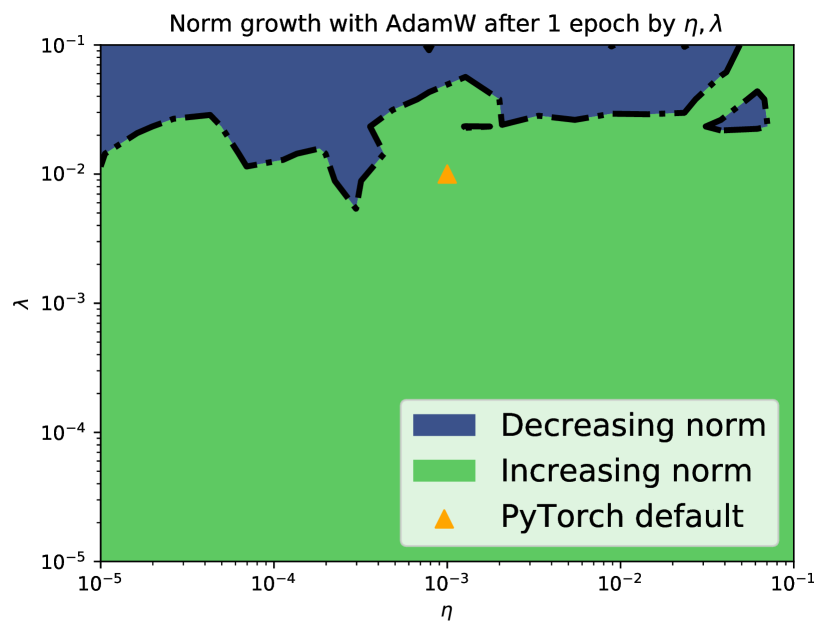
Figure 6: Norm growth over the first epoch, varying $\eta,\lambda$. The triangle shows the default AdamW hyperparameters in PyTorch.

References

- Arora et al. (2019) Sanjeev Arora, Nadav Cohen, Wei Hu, and Yuping Luo. 2019. Implicit regularization in deep matrix factorization.
- Bhattamishra et al. (2020) Satwik Bhattamishra, Kabir Ahuja, and Navin Goyal. 2020. On the Ability and Limitations of Transformers to Recognize Formal Languages. In Proceedings of the 2020 Conference on Empirical Methods in Natural Language Processing (EMNLP), pages 7096–7116, Online. Association for Computational Linguistics.
- Chomsky (1956) N. Chomsky. 1956. Three models for the description of language. IRE Transactions on Information Theory, 2(3):113–124.
- Correia et al. (2019) Gonçalo M. Correia, Vlad Niculae, and André F. T. Martins. 2019. Adaptively sparse transformers. In Proceedings of the 2019 Conference on Empirical Methods in Natural Language Processing and the 9th International Joint Conference on Natural Language Processing (EMNLP-IJCNLP), pages 2174–2184, Hong Kong, China. Association for Computational Linguistics.
- Devlin et al. (2019) Jacob Devlin, Ming-Wei Chang, Kenton Lee, and Kristina Toutanova. 2019. BERT: Pre-training of deep bidirectional transformers for language understanding. In Proceedings of the 2019 Conference of the North American Chapter of the Association for Computational Linguistics: Human Language Technologies, Volume 1 (Long and Short Papers), pages 4171–4186, Minneapolis, Minnesota. Association for Computational Linguistics.
- Ebrahimi et al. (2020) Javid Ebrahimi, Dhruv Gelda, and Wei Zhang. 2020. How can self-attention networks recognize Dyck-n languages? In Findings of the Association for Computational Linguistics: EMNLP 2020, pages 4301–4306, Online. Association for Computational Linguistics.
- Francis and Kučera (1989) Winthrop Nelson Francis and Henry Kučera. 1989. Manual of information to accompany a standard corpus of present-day edited American English, for use with digital computers. Brown University, Department of Linguistics.
- Goldblum et al. (2020) Micah Goldblum, Jonas Geiping, Avi Schwarzschild, Michael Moeller, and Tom Goldstein. 2020. Truth or backpropaganda? an empirical investigation of deep learning theory. In International Conference on Learning Representations.
- Gunasekar et al. (2017) Suriya Gunasekar, Blake Woodworth, Srinadh Bhojanapalli, Behnam Neyshabur, and Nathan Srebro. 2017. Implicit regularization in matrix factorization.
- Hahn (2020) Michael Hahn. 2020. Theoretical limitations of self-attention in neural sequence models. Transactions of the Association for Computational Linguistics, 8:156–171.
- Ji and Telgarsky (2020) Ziwei Ji and Matus Telgarsky. 2020. Directional convergence and alignment in deep learning. In Advances in Neural Information Processing Systems, volume 33, pages 17176–17186. Curran Associates, Inc.
- Kirov and Frank (2012) Christo Kirov and Robert Frank. 2012. Processing of nested and cross-serial dependencies: an automaton perspective on SRN behaviour. Connection Science, 24(1):1–24.
- Li and Arora (2019) Zhiyuan Li and Sanjeev Arora. 2019. An exponential learning rate schedule for deep learning. In Proc. of ICLR.
- Liu et al. (2019) Yinhan Liu, Myle Ott, Naman Goyal, Jingfei Du, Mandar Joshi, Danqi Chen, Omer Levy, Mike Lewis, Luke Zettlemoyer, and Veselin Stoyanov. 2019. RoBERTa: A robustly optimized BERT pretraining approach.
- Loshchilov and Hutter (2017) Ilya Loshchilov and Frank Hutter. 2017. Fixing weight decay regularization in adam. CoRR, abs/1711.05101.
- Lovering et al. (2021) Charles Lovering, Rohan Jha, Tal Linzen, and Ellie Pavlick. 2021. Predicting inductive biases of pre-trained models. In International Conference on Learning Representations.
- Lyu and Li (2019) Kaifeng Lyu and Jian Li. 2019. Gradient descent maximizes the margin of homogeneous neural networks.
- Marcus et al. (1993) Mitchell P. Marcus, Beatrice Santorini, and Mary Ann Marcinkiewicz. 1993. Building a large annotated corpus of English: The Penn Treebank. Computational Linguistics, 19(2):313–330.
- Merity et al. (2016) Stephen Merity, Caiming Xiong, James Bradbury, and Richard Socher. 2016. Pointer sentinel mixture models.
- Merrill (2019) William Merrill. 2019. Sequential neural networks as automata. Proceedings of the Workshop on Deep Learning and Formal Languages: Building Bridges.
- Merrill (2020) William Merrill. 2020. On the linguistic capacity of real-time counter automata.
- Merrill et al. (2020) William. Merrill, Gail Garfinkel Weiss, Yoav Goldberg, Roy Schwartz, Noah A. Smith, and Eran Yahav. 2020. A formal hierarchy of RNN architectures. In Proc. of ACL.
- Nacson et al. (2019) Mor Shpigel Nacson, Suriya Gunasekar, Jason D. Lee, Nathan Srebro, and Daniel Soudry. 2019. Lexicographic and depth-sensitive margins in homogeneous and non-homogeneous deep models.
- Poggio et al. (2019) Tomaso Poggio, Andrzej Banburski, and Qianli Liao. 2019. Theoretical issues in deep networks: Approximation, optimization and generalization.
- Poggio et al. (2020) Tomaso Poggio, Qianli Liao, and Andrzej Banburski. 2020. Complexity control by gradient descent in deep networks. Nature communications, 11(1):1–5.
- Raffel et al. (2019) Colin Raffel, Noam Shazeer, Adam Roberts, Katherine Lee, Sharan Narang, Michael Matena, Yanqi Zhou, Wei Li, and Peter J. Liu. 2019. Exploring the limits of transfer learning with a unified text-to-text transformer.
- Razin and Cohen (2020) Noam Razin and Nadav Cohen. 2020. Implicit regularization in deep learning may not be explainable by norms.
- Rogers et al. (2020) Anna Rogers, Olga Kovaleva, and Anna Rumshisky. 2020. A primer in BERTology: What we know about how BERT works. Transactions of the Association for Computational Linguistics, 8:842–866.
- Shazeer and Stern (2018) Noam Shazeer and Mitchell Stern. 2018. Adafactor: Adaptive learning rates with sublinear memory cost. CoRR, abs/1804.04235.
- Shibata et al. (2020) Chihiro Shibata, Kei Uchiumi, and Daichi Mochihashi. 2020. How LSTM encodes syntax: Exploring context vectors and semi-quantization on natural text.
- Siegelmann and Sontag (1992) Hava T. Siegelmann and Eduardo D. Sontag. 1992. On the computational power of neural nets. In Proc. of COLT, pages 440–449.
- Suzgun et al. (2019a) Mirac Suzgun, Yonatan Belinkov, Stuart Shieber, and Sebastian Gehrmann. 2019a. LSTM networks can perform dynamic counting. In Proceedings of the Workshop on Deep Learning and Formal Languages: Building Bridges, pages 44–54.
- Suzgun et al. (2019b) Mirac Suzgun, Sebastian Gehrmann, Yonatan Belinkov, and Stuart M. Shieber. 2019b. Memory-augmented recurrent neural networks can learn generalized Dyck languages.
- Vaswani et al. (2017) Ashish Vaswani, Noam Shazeer, Niki Parmar, Jakob Uszkoreit, Llion Jones, Aidan N. Gomez, Lukasz Kaiser, and Illia Polosukhin. 2017. Attention is all you need.
- Weiss et al. (2018) Gail Weiss, Yoav Goldberg, and Eran Yahav. 2018. On the practical computational power of finite precision RNNs for language recognition.
- Wolf et al. (2019) Thomas Wolf, Lysandre Debut, Victor Sanh, Julien Chaumond, Clement Delangue, Anthony Moi, Pierric Cistac, Tim Rault, R’emi Louf, Morgan Funtowicz, and Jamie Brew. 2019. Huggingface’s transformers: State-of-the-art natural language processing. ArXiv, abs/1910.03771.
- Xiong et al. (2020) Ruibin Xiong, Yunchang Yang, Di He, Kai Zheng, Shuxin Zheng, Chen Xing, Huishuai Zhang, Yanyan Lan, Liwei Wang, and Tie-Yan Liu. 2020. On layer normalization in the transformer architecture.
- Yang et al. (2019) Zhilin Yang, Zihang Dai, Yiming Yang, Jaime Carbonell, Ruslan Salakhutdinov, and Quoc V. Le. 2019. Xlnet: Generalized autoregressive pretraining for language understanding.
- Yun et al. (2020) Chulhee Yun, Srinadh Bhojanapalli, Ankit Singh Rawat, Sashank Reddi, and Sanjiv Kumar. 2020. Are transformers universal approximators of sequence-to-sequence functions? In International Conference on Learning Representations.