On the Robustness of Winners:
Counting Briberies in Elections

Abstract

We study the parameterized complexity of counting variants of Swap- and Shift-Bribery problems, focusing on the parameterizations by the number of swaps and the number of voters. We show experimentally that Swap-Bribery offers a new approach to the robustness analysis of elections.

1 Introduction

Consider a university department which is about to hire a new professor. There are $m$ candidates and the head of the department decided to choose the winner by Borda voting. Each faculty member (i.e., each voter) ranked the candidates from the most to the least appealing one, each candidate received $m-i$ points for each vote where he or she was ranked as the $i$-th best, and the candidate with the highest score was selected. However, after the results were announced, some voters started wondering if, perhaps, some other voters accidently “misranked” some of the candidates (worrying about mistakes in the votes is an old democratic tradition). For instance, if some voter viewed two candidates as very similar, then he or she could have ranked them either way, depending on an impulse. Or, some voter would have ranked two candidates differently if he or she had more information on their merits (this is particularly likely for low-ranked candidates). It is, thus, natural to ask for the probability of changing the election outcome by making some random swaps. Indeed, this approach was recently pursued by Baumeister and Hogrebe [3] and we follow-up on it, but with a somewhat different focus (we will discuss this difference together with other related work).

Specifically, for each $r\in\mathbb{N}$ and each candidate $c$, we let $P_{c}(r)$ be the probability that $c$ wins an election obtained by making $r$ random swaps of candidates ranked on adjacent positions in the votes (we refer to such elections as being at swap distance $r$ from the original one). Such values can be quite useful. For example, if for each $r$ we had (some estimate of) the probability that in total there are $r$ accidental swaps in the votes, then we could compute the probability of each candidate’s victory. If it were small for the original winner, then we might want to recount the votes or reexamine the election process. The values $P_{c}(r)$ are also useful without the distribution of $r$’s. For example, we may want to find the smallest number of swaps for which the probability of the original winner’s victory drops below some value (such as 50%) or for which he or she is no longer the most probable winner. As we show in our experiments, this approach provides new insights on the robustness of election results.

To determine the value $P_{c}(r)$, we need to divide the number of elections at swap distance $r$ where $c$ wins, by the total number of elections at this distance. While computing the latter is easy—at least in the sense that there is a polynomial-time algorithm for this task—computing the former requires solving the counting variant of the Swap-Bribery problem (denoted #Swap-Bribery). Briefly put, in the decision variant of the problem, we ask if it is possible to ensure that a designated candidate wins a given election by making $r$ swaps of adjacent candidates in the votes (we assume the unit prices setting; see Section 2). In the counting variant, we ask how many ways there are to achieve this effect (using exactly $r$ swaps). Unfortunately, already the decision variant is ${\mathrm{NP}}$-hard for many voting rules, and we show that the counting one is hard even for Plurality. On the positive side, we can get a good estimate of $P_{c}(r)$ by sampling.

We also consider the Shift-Bribery problem, a variant of Swap-Bribery where we can only shift the designated candidate forward (in the constructive case) or backward (in the destructive one, where the goal is to ensure that the designated candidate loses). These problems also can be used to evaluate robustness of election results but, to maintain focus, in our experiments we only consider Swap-Bribery. Yet, we include Shift-Bribery in our complexity analysis because it illustrates some interesting phenomena.

1.1 Main Contributions

We focus on #Swap- and #Shift-Bribery for the Plurality and Borda voting rules (for unit prices). We consider their computational complexity for parameterizations by the number of unit swaps/shifts (which we refer to as the swap/shift radius) and by the number of voters (see Table 1). We also present experiments, where we use #Swap-Bribery to evaluate the robustness of election results. Our main results are as follows:

1. For Plurality, Swap-Bribery is known to be in ${\mathrm{P}}$, but we show that the counting variant is $\#{\mathrm{P}}$-hard, and even $\#{\mathsf{W[1]}}$-hard for the parameterization by the swap radius.

2. For Borda, hardness results for #Swap-Bribery follow from those for #Shift-Bribery, which themselves are intriguing: E.g., the destructive variant parameterized by the shift radius is $\#{\mathsf{W[1]}}$-hard, but the constructive one is in ${\mathrm{FPT}}$; yet, in the decision setting the former is easier.

3. Using sampling, we estimate the candidate’s winning probabilities in elections from a dataset generated by Szufa et al. [31]. One of the high-level conclusions is that the score differences between the election winners and the runners-up can be quite disconnected from their strengths (measured using #Swap-Bribery).

Some proofs and analyses are available in the appendix.

	Plurality		Borda
	decision	counting	decision	counting
		$\#{\mathrm{P}}$-hard	${\mathrm{NP}}$-hard	$\#{\mathrm{P}}$-hard
Swap-Bribery	${\mathrm{P}}$	$\#{\mathsf{W[1]}}$-hard$(r)$	${\mathrm{FPT}}(r)$	?
		${\mathrm{FPT}}(n)$	${\mathsf{W[1]}}$-hard$(n)$	$\#{\mathsf{W[1]}}$-hard$(n)$
Constructive			${\mathrm{NP}}$-hard	$\#{\mathrm{P}}$-hard
Shift-Bribery	${\mathrm{P}}$	${\mathrm{P}}$	${\mathrm{FPT}}(r)$	${\mathrm{FPT}}(r)$
			${\mathsf{W[1]}}$-hard$(n)$	$\#{\mathsf{W[1]}}$-hard$(n)$
1-5 Destructive				$\#{\mathrm{P}}$-hard
Shift-Bribery	${\mathrm{P}}$	${\mathrm{P}}$	${\mathrm{P}}$	$\#{\mathsf{W[1]}}$-hard$(r)$
				$\#{\mathsf{W[1]}}$-hard$(n)$

Table 1: (Parameterized) complexity of Swap- and Shift-Bribery with unit prices; $r$ and $n$ refer to the parameterizations by the swap/shift radius and by the number of voters, respectively. Results for the counting variants are due to this paper (however, see also the work of Baumeister and Hogrebe [3] for results related to $\#{\mathrm{P}}$-hardness of Swap-Bribery); the other ones are due to Elkind et al. [16], Bredereck et al. [8, 6], and Kaczmarczyk and Faliszewski [21].

1.2 Related Work

Our work is most closely related to the papers of Hazon et al. [20], Bachrach et al. [1], and Baumeister and Hogrebe [3]. Like us, their authors study the complexity of computing the probability that a given candidate wins, provided that the votes may change according to some probability distribution. In particular, Hazon et al. [20] assume that each voter is endowed with an explicitly encoded list of possible votes, each with its probability of being cast, Bachrach et al. [1] consider elections where the votes are partial and all completions are equally likely, and Baumeister and Hogrebe [3] consider both these models, as well as a third one, where the votes may change according to the Mallows noise model [26].

Under the Mallows model, we are given an election—to which we refer as the original one—and a parameter $\phi$. Each possible election is associated with weight $\phi^{d}$, where $d$ is its swap distance to the original one, and the probability of drawing a particular election is proportional to its weight. Thus, the Mallows model is very closely related to our approach of counting solutions for Swap Bribery. Indeed, the only difference is that we take the number of swaps as part of the input (so, intuitively, we view each election at this swap distance as equally likely), and in the Mallows model Baumeister and Hogrebe [3] take $\phi$ as part of the input and consider all possible swap distances (but the probability of drawing an election at a given distance is weighted according to the Mallows model with $\phi$ as the parameter).

There are two methodological differences between our work and the three above-discussed papers. Foremost, we provide a detailed experimental analysis showing that counting variants of Swap-Bribery are indeed helpful for evaluating robustness of election winners. In contrast, Bachrach et al. [1] and Baumeister and Hogrebe [3] focus entirely on the complexity analysis, whereas Hazon et al. [20] also provide experiments, but their focus is on the running time and memory consumption of their algorithm.

The second difference regards the use of parameterized complexity theory. Indeed, we believe that we are the first to use a parameterized counting complexity analysis—with an explicit focus on establishing ${\mathrm{FPT}}$ and $\#{\mathsf{W[1]}}$-hardness results—in the context of elections. However, we do mention that Hazon et al. [20] and Baumeister and Hogrebe [3] consider settings where either the numbers of candidates or the numbers of voters are fixed constants, so, effectively, they provide ${\mathrm{XP}}$ algorithms.

Swap- and Shift-Bribery were introduced by Elkind et al. [16]. Various authors studied these problems for different voting rules (see, e.g., the works of Maushagen et al. [27] and Zhou and Guo [37] regarding iterative elections), sought approximation algorithms [15, 18], established parameterized complexity results [14, 8, 23], considered restricted preference domains [17], and extended the problem in various ways [6, 21, 4, 36]. The idea of using Swap-Bribery to measure the robustness of election results is due to Shiryaev et al. [30], but is also closely related to computing the margin of victory [25, 11, 35, 10]; recently it was also applied to committee elections [7].

So far, the complexity of counting problems received fairly limited attention in the context of elections. In addition to the works of Hazon et al. [20], Bachrach et al. [1] and Baumeister and Hogrebe [3], we mention two more: Wojtas and Faliszewski [34] studied the complexity of counting solutions for control problems, whereas Kenig and Kimelfeld [22] followed up on the work of Bachrach et al. [1] and provided approximation algorithms for their setting.

2 Preliminaries

For each integer $k$, by $[k]$ we mean the set $\{1,\ldots,k\}$.

Elections. An election $E=(C,V)$ consists of a set $C=\{c_{1},\ldots,c_{m}\}$ of candidates and a collection $V=(v_{1},\ldots,v_{n})$ of voters. Each voter $v_{i}$ has a preference order, which ranks all the candidates from the most to the least desired one (we sometimes refer to preference orders as votes). For a voter $v_{i}$, we write $v_{i}\colon c_{1}\succ c_{2}\succ\cdots\succ c_{m}$ to indicate that he or she ranks $c_{1}$ first, then $c_{2}$, and so on. If we put a subset of candidates in such a description of a preference order, then we mean listing its members in an arbitrary order.

Voting Rules. A voting rule $\mathcal{R}$ is a function that, given an election, returns a set of candidates that tie as winners. We focus on Plurality and Borda, which assign scores to the candidates and select those with the highest ones. Under Plurality, each voter gives one point to the top-ranked candidate. Under Borda, each voter gives $|C|-1$ points to the top-ranked candidate, $|C|-2$ points to the next one, and so on. We write $\operatorname{score}_{E}(c)$ to denote the score of candidate $c$ in election $E$ (the voting rule will be clear from the context).

Swap Distance. Let $u$ and $v$ be two votes over the same candidate set. The swap distance between $u$ and $v$, denoted $d_{\mathrm{sw}}(u,v)$, is the length of the shortest sequence of swaps of adjacent candidates whose application transforms $u$ into $v$. Given elections $E=(C,V)$ and $E^{\prime}=(C,V^{\prime})$, where $V=(v_{1},\ldots,v_{n})$ and $V^{\prime}=(v^{\prime}_{1},\ldots,v^{\prime}_{n})$, their swap distance is $\sum_{i=1}^{n}d_{\mathrm{sw}}(v_{i},v^{\prime}_{i})$. By $R(E,r)$, we denote the set of elections that are at swap distance $r$ from $E$.

Swap- and Shift-Bribery. Let $\mathcal{R}$ be a voting rule. In the decision variant of the $\mathcal{R}$ Swap-Bribery problem, we are given an election $E$, a designated candidate $p$, and a budget $r$. Further, for each voter and each two candidates $c$ and $d$, we have a nonnegative price $\pi_{v}(c,d)$ for swapping them in $v$’s preference order (a swap is legal if at the time of its application $c$ and $d$ are adjacent). We ask if there is an election $E^{\prime}$ where $p$ is an $\mathcal{R}$-winner, such that $E^{\prime}$ can be obtained from $E$ by performing a sequence of legal swaps of cost at most $r$. In the counting variant, we ask for the number of such elections, and we require the cost of swaps to be exactly $r$ (the last condition is for our convenience and all our results would still hold if we asked for cost at most $r$; the same would be true if instead of counting elections where $p$ won, we would count those where he or she lost). Since we are interested in computing the candidates’ probabilities of victory in elections at a given swap distance, we focus on the case where each swap has the same, unit price; thus, we usually refer to $r$ as the swap radius and not as the budget.

Constructive Shift-Bribery is a variant of Swap-Bribery where all swaps must involve the designated candidate, shifting him or her forward. Destructive Shift-Bribery is defined analogously, except that our goal is to preclude the designated candidate’s victory, and we can only shift him or her backward [21]. Counting variants are defined in a natural way. We focus on the case where each unit shift has a unit price and we speak of shift radius $r$ instead of budget or swap radius.

Counting Complexity. We assume basic familiarity with (parameterized) complexity theory, including classes ${\mathrm{P}}$, ${\mathrm{NP}}$, ${\mathrm{FPT}}$, and ${\mathsf{W[1]}}$, and reducibility notions.

Let X be a decision problem from ${\mathrm{NP}}$, where for each instance we ask if there exists some mathematical object with a given property. In its counting variant, traditionally denoted #X, we ask for the number of such objects. For example, in Matching we are given an integer $k$ and a bipartite graph $G$—with vertex set $U(G)\uplus V(G)$ and edge set $E(G)$—and we ask if $G$ contains a matching of size $k$ (i.e., a set of $k$ edges, where no two edges touch the same vertex). In #Matching we ask how many such matchings exist.

The class $\#{\mathrm{P}}$ is the counting analog of ${\mathrm{NP}}$; a problem belongs to $\#{\mathrm{P}}$ if it can be expressed as the task of counting accepting computations of a nondeterministic polynomial-time Turing machine. We say that a counting problem #A (polynomial-time) Turing reduces to #B if there exists an algorithm that solves #A in polynomial time, provided that it has oracle access to #B. A problem is $\#{\mathrm{P}}$-hard if every problem from $\#{\mathrm{P}}$ Turing reduces to it. While Matching is in ${\mathrm{P}}$, it is well known that #Matching is $\#{\mathrm{P}}$-hard, and even $\#{\mathrm{P}}$-complete [32].

$\#{\mathsf{W[1]}}$ relates to ${\mathsf{W[1]}}$ in the same way as $\#{\mathrm{P}}$ relates to ${\mathrm{NP}}$. As examples of $\#{\mathsf{W[1]}}$-hard problems, we mention counting size-$k$ cliques in a graph, parameterized by $k$ [19] and #Matching, parameterized by the size of the matching [13]. Formally, $\#{\mathsf{W[1]}}$-hardness is defined using a slightly more general notion of a reduction, but for our purposes polynomial-time Turing reductions (where the parameters in the queried instances are bounded by a function of the parameter in the input instance) will suffice.

3 Algorithms and Complexity Results

In this section, we present our results regarding the complexity of #Swap- and #Shift-Bribery. We first consider Plurality, mostly focusing on the former problem, and then discuss Borda, mostly focusing on the latter.

3.1 Plurality and #Swap-Bribery

We start with bad news. While there is a polynomial-time algorithm for the decision variant of Plurality Swap-Bribery [16], the counting variant is intractable, even with unit prices (for the $\#{\mathrm{P}}$-hardness, a related result is reported by Baumeister and Hogrebe [3]).

Theorem 1.

Plurality #Swap-Bribery is $\#{\mathrm{P}}$-hard and $\#{\mathsf{W[1]}}$-hard for the parameterization by the swap radius, even for unit prices.

Proof.

We give a reduction from #Matching. We will use a swap radius bounded by a function of the desired matching size, so we will obtain both $\#{\mathrm{P}}$- and $\#{\mathsf{W[1]}}$-hardness.

Let $(G,k)$ be an instance of #Matching, where $G$ is a bipartite graph with vertex set $U(G)\uplus V(G)$ and $k$ is the size of the matchings that we are to count. Assume that $U(G)=\{u_{1},\ldots,u_{n}\}$, $V(G)=\{v_{1},\ldots,v_{n}\}$, and $k\leq n$. To form an election, we let the candidate set be $C:=U(G)\uplus V(G)\uplus\{p,a,b\}\uplus X$, where $X:=\{x_{1},\ldots,x_{3k+1}\}$. The candidates in $U(G)\uplus V(G)$ will model the graph, $p$ will be our designated candidate, $a$ and $b$ will control the size of the matching, and the candidates in $X$ will block undesirable swaps. We will have the following scores of the candidates:

$$\forall c\in C\setminus\{a,b\}\colon \operatorname{score}_{E}(c)=n,$$

$$\operatorname{score}_{E}(a)=n-k,\ \operatorname{score}_{E}(b)=n+k.$$

We form the following four groups of voters:

1. For each edge $\{u_{i},v_{j}\}\in E(G)$, there is an edge voter $e_{ij}$ with preference order $e_{ij}\colon u_{i}\succ v_{j}\succ X\succ\cdots.$

2. For each $j\in[n]$, we have an $a$-voter $a_{j}$ with preference order $a_{j}\colon v_{j}\succ a\succ X\succ\cdots.$

3. For each $i\in[n]$, we have a $b$-voter $b_{i}$ with preference order $b_{i}\colon b\succ u_{i}\succ X\succ\cdots.$

4. Finally, the score voters implement the desired Plurality scores. For each candidate $c\in U(G)\cup V(G)\cup\{p\}$, there are exactly as many voters with preference order $c\succ X\succ\cdots$ as necessary to ensure that in total $c$ has score $n$. Similarly, for each $x_{i}\in X$ there are $n$ voters with preference order $x_{i}\succ X\setminus\{x_{i}\}\succ\cdots$. There are also $n-k$ voters with preference order $a\succ X\succ\cdots$ and $k$ voters with preference order $b\succ X\succ\cdots$.

Let $E$ be an election with the above-described candidates and voters. We form an instance $I$ of Plurality #Swap-Bribery with this election, unit prices, and swap radius $r:=3k$. Then, we make an oracle query for $I$ and return its answer. In the remainder of the proof, we argue that this answer is equal to the number of size-$k$ matchings in $G$. The idea is that to make $p$ a winner, we have to transfer $k$ points from $b$ to $a$ via swaps that correspond to a matching.

Let $E^{\prime}$ be some election in $R(E,r)$, i.e., an election at swap distance $r$ from $E$, where $p$ wins. We note that $p$ and the candidates from $X$ have score $n$ in $E^{\prime}$ (indeed, in elections from $R(E,r)$, $p$ has score at most $n$ and the average score of the candidates in $X$ is at least $n$). Further, in $E^{\prime}$ each edge voter, $a$-voter, and $b$-voter either ranks on top the same candidate as in $E$, or the candidate that he or she ranked second in $E$ (otherwise some candidate in $X$ would have score above $n$). We call this the top-two rule.

Since $b$ must have at most $n$ points in $E^{\prime}$, by the top-two rule, there must be at least $k$ $b$-voters that rank members of $U(G)$ on top. Let $U_{b}$ be the set of these members of $U(G)$. As each member of $U(G)$ can be swapped with $b$ at most once in the $b$-votes, we have $|U_{b}|\geq k$.

Compared to $E$, in $E^{\prime}$ each member of $U_{b}$ gets an additional point from the $b$-voters. Thus, for each $u_{i}\in U_{b}$ there must be a voter that ranked $u_{i}$ on top in $E$ but does not do so in $E^{\prime}$. By the top-two rule, this must be an edge voter. Let $M$ be the set of pairs $\{u_{i},v_{j}\}$ such that in $E$ edge voter $e_{ij}$ ranks $u_{i}$ on top, but in $E^{\prime}$ he or she ranks $v_{j}$ on top. Naturally, we must have $|M|\geq|U_{b}|$.

For each pair $\{u_{i},v_{j}\}\in M$, there must be a voter who swapped $v_{j}$ out of the top position in $E^{\prime}$, because otherwise $v_{j}$ would have more than $n$ points. By similar arguments as before, this must be voter $a_{j}$. Let $V_{a}$ be the set of those members of $V(G)$ that in $E^{\prime}$ are swapped out of the top positions in the $a$-votes. It must be that $|V_{a}|\geq|M|$.

Altogether, we have $|V_{a}|\geq|M|\geq|U_{b}|\geq k$ and, in fact, each of these sets must have exactly $k$ elements (because their elements correspond to unique swaps). Further, $M$ is a matching. If it were not, then some member of $U(G)\uplus V(G)$ would appear in two pairs in $M$, but then we would have to have two $a$-voters or two $b$-voters that corresponded to this candidate, which is not possible in our construction.

This way we have shown that for each election in $R(E,r)$ where $p$ wins, there is a corresponding size-$k$ matching. As the other direction is immediate, the proof is complete. ∎

A natural way to circumvent such intractability results is to seek ${\mathrm{FPT}}$ algorithms parameterized by the number of candidates or by the number of voters. For the former, one typically expresses Swap-Bribery problems as integer linear programs (ILPs) and invokes the classic algorithm of Lenstra, Jr. [24], or some more recent one; see, e.g., the work of Knop et al. [23]. Unfortunately, counting analogs of these algorithms, dating back to the seminal work of Barvinok [2], have ${\mathrm{XP}}$ running times and cannot be used for our purpose. Thus, we leave the complexity of our problems parameterized by the number of candidates open. Yet, for unit prices we do show an ${\mathrm{FPT}}$ algorithm parameterized by the number of voters.

Theorem 2.

For unit prices, Plurality #Swap-Bribery parameterized by the number of voters is in ${\mathrm{FPT}}$.

Proof sketch.

Consider an instance $I$ of Plurality #Swap-Bribery with election $E=(C,V)$, where $C=\{c_{1},c_{2},\ldots,c_{m}\}$ and $V$ contains $n$ voters. Let $r$ be the swap radius and, w.l.o.g., let $p=c_{1}$ be the designated candidate.

The core idea is to go over all possible sequences $\mathcal{V}=(V_{1},\ldots,V_{m^{\prime}})$ such that (a) $m^{\prime}\leq\min(m,n)$, (b) each $V_{i}$ is a subcollection of $V$ (consisting of not necessarily consecutive voters), (c) each voter belongs to exactly one $V_{i}$, and (d) group $V_{1}$ has at least as many voters as every other group. For each such sequence, we solve the following global counting problem: Count the number of ways to perform exactly $r$ swaps so that (i) within each $V_{i}$, each two voters rank the same candidate, denoted $c(V_{i})$, on top, (ii) all voters in $V_{1}$ rank $p$ on top (i.e., $c(V_{1})=p$), and (iii) for each two groups $V_{i}$ and $V_{i^{\prime}}$, where $i<i^{\prime}$ and we have $c_{j}=c(V_{i})$ and $c_{j^{\prime}}=c(V_{i^{\prime}})$, it holds that $j<j^{\prime}$. These conditions ensure that after performing the swaps, each group votes for a different candidate, each candidate $c(V_{i})$ receives exactly $|V_{i}|$ points, and $p$ wins. One can verify that every solution for our input instance corresponds to exactly one sequence $\mathcal{V}$. In other words, to obtain the answer for $I$, we need to sum up the answers for the global counting problems for each $\mathcal{V}$.

To solve a given global counting problem in polynomial time, we define $T[i,\ell,s]$ to be the number of ways to perform exactly $s$ swaps within the first $i$ voter groups, so that conditions (i)–(iii) hold for $V_{1},\ldots V_{i}$, and so that $c(V_{i})=c_{\ell}$. We compute these values using dynamic programming (which requires solving a local counting problem, also via dynamic programming, to count for each voter group the number of ways to ensure that all its members rank a given candidate on top). The solution for the global counting problem is then $\sum_{\ell\leq m}T[m^{\prime},\ell,r]$.

As the number of global counting problems to solve is bounded by a function of $n$, and each such problem is solved in polynomial time, the algorithm runs in ${\mathrm{FPT}}$ time with respect to the number of voters. ∎

The restriction to unit prices in Theorem 2 is necessary. Otherwise, a reduction from the problem of counting linear extensions of a partially ordered set by Brightwell and Winkler [9] shows $\#{\mathrm{P}}$-hardness even for a single voter.

Theorem 3.

Plurality #Swap-Bribery is $\#{\mathrm{P}}$-hard even for a single voter and unary-encoded prices.

We conclude with a brief mention of #Shift-Bribery. Both the constructive and the destructive variant are in ${\mathrm{P}}$, even with arbitrary unary-encoded prices (for the binary encoding, $\#{\mathrm{P}}$-hardness follows by a reduction from #Partition). Our algorithms use dynamic programming over groups of voters with the same candidate as their top choice.

Theorem 4.

For unary-encoded prices, both the constructive and the destructive variant of Plurality #Shift-Bribery are in ${\mathrm{P}}$.

3.2 Borda and #Shift-Bribery

Our results for Borda #Swap-Bribery follow from those for #Shift-Bribrey, so we discuss the latter problem first.

In the decision setting, the constructive variant of Borda Shift-Bribery is ${\mathrm{NP}}$-hard (and is in ${\mathrm{FPT}}$ when parameterized by the shift radius, but is ${\mathsf{W[1]}}$-hard for the number of voters), whereas the destructive variant is in ${\mathrm{P}}$. In the counting setting, both variants are $\#{\mathrm{P}}$-hard and $\#{\mathsf{W[1]}}$-hard for the parameterization by the number of voters; the result for the constructive case follows from a proof for the decision variant due to Bredereck et al. [6] and for the destructive case, we use a similar approach with a few tricks on top.

Theorem 5.

Both the constructive and the destructive variant of Borda #Shift-Bribery are $\#{\mathrm{P}}$-hard and $\#{\mathsf{W[1]}}$-hard when parameterized by the number of voters.

More surprisingly, for the parameterization by the shift radius, the constructive variant is in ${\mathrm{FPT}}$ and the destructive variant is $\#{\mathsf{W[1]}}$-hard. Not only does the problem that was easier in the decision setting now became harder, but also—to the best of our knowledge—it is the first example where a destructive variant of an election-related problem is harder than the constructive one. Yet, Shift-Bribery is quite special as the two variants differ both in the goal (i.e, whether we want the designated candidate to win or not) and in the available actions (shifting the designated candidate forward or backward; typically, destructive voting problems have the same sets of actions as the constructive ones).

The ${\mathrm{FPT}}$ algorithm for the constructive case relies on the fact that if we can ensure victory of the designated candidate by shifting him or her by $r$ positions forward, then there are at most $r$ candidates that we need to focus on (the others will be defeated irrespective what exact shifts we make). There are no such bounds in the destructive setting.

Theorem 6.

Parameterized by the shift radius, Borda #Constructive Shift-Bribery is in ${\mathrm{FPT}}$ (for unary-encoded prices), but the destructive variant is $\#{\mathsf{W[1]}}$-hard, even for unit prices.

Proof (destructive case).

We give a polynomial-time Turing reduction from #Matching to Borda #Destructive Shift-Bribery. Let $(G,k)$ be an instance of #Matching, where $G$ is a bipartite graph with vertex set $U(G)\uplus V(G)$, and $k$ is a positive integer. Without loss of generality, we assume that $U(G)=\{u_{1},\ldots,u_{n}\}$, $V(G)=\{v_{1},\ldots,v_{n}\}$, and $k\leq n$.

Our reduction proceeds as follows. First, we form the set of relevant candidates $R:=\{d,p\}\uplus U(G)\uplus V(G)$, where $d$ is the designated candidate. Moreover, for each relevant candidate $r\in R$, we form a set $D(r)$ of $3k+1$ dummy ones. We will form an election $E$, where these candidates will have the following Borda scores ($X$ is some positive integer, whose value depends on the specifics of the construction; we will be counting ways in which $d$ can cease to be a winner by shifting him or her backward by $3k$ positions):

$$\operatorname{score}_{E}(d)=X+3k,$$ (1)

$$\operatorname{score}_{E}(p)=X-k+1,$$ (2)

$$\operatorname{score}_{E}(u_{1})=\cdots=\operatorname{score}_{E}(u_{n})=X-1,$$ (3)

$$\operatorname{score}_{E}(v_{1})=\cdots=\operatorname{score}_{E}(v_{n})=X-1,\text{ and}$$ (4)

$$\text{each dummy candidate has score at most $X-3k-1$}.$$ (5)

Election $E$ contains the following voters:

1. For each edge $e=\{u_{i},v_{j}\}$ of the input graph, there is an edge voter $v_{e}$ with preference order $v_{e}\colon d\succ u_{i}\succ v_{j}\succ p\succ D(p)\succ\cdots.$

2. There is a group of voters who ensure that the scores are as described above. They rank at least $3k$ dummy candidates between each two relevant ones (so shifting $d$ by $3k$ positions back cannot change the score of another relevant candidate).

   More precisely, we have a group of score voters, who ensure that conditions (1)–(5) hold. Let $\pi$ be the following preference order, giving the basic pattern for forming all score voters:

   $$\pi\colon D(u_{1})\succ u_{1}\succ\cdots\succ D(u_{n})\succ u_{n}\succ D(p)\succ p\succ$$

   $$D(v_{1})\succ v_{1}\succ\cdots\succ D(v_{n})\succ v_{n}\succ D(d)\succ d.$$

   The crucial feature of $\pi$ is that relevant candidates are separated from each other with at least $3k+1$ dummy ones; their particular order is not important. For each relevant candidate $c\in R$, let ${{\mathrm{inc}}}(c)$ be a pair of preference orders where one is equal to reversed $\pi$, and the other is identical to $\pi$ except that $c$ is shifted one position forward. By adding a pair of voters with preference orders ${{\mathrm{inc}}}(c)$ to the election, we increase the score of $c$ by $|C|$, the scores of the other relevant candidates by $|C|-1$, and the scores of the dummy candidates by at most $|C|-1$. For each relevant candidate $c\in R$, we add polynomially many such pairs of voters—the polynomial is with respect to $n$ and $k$—as follows:

   1. For each relevant candidate $c\in R$ we add the smallest number of pairs of voters ${{\mathrm{inc}}}(c)$ so that, taken together with the edge voters, all relevant candidates have identical scores and each relevant candidate has a higher score than each dummy candidate.

   2. For each relevant candidate $c\in R$, we add $3k+1$ pairs of voters ${{\mathrm{inc}}}(c)$ (this ensures that, in total, each relevant candidate has at least $3k$ points more than each dummy candidate).

   3. We add $4k$ pairs of voters ${{\mathrm{inc}}}(d)$, one pair of voters ${{\mathrm{inc}}}(p)$, and for each $i\in[n]$, we add $k-1$ pairs of voters ${{\mathrm{inc}}}(u_{i})$ and $k-1$ pairs of voters ${{\mathrm{inc}}}(v_{i})$ (this ensures that the scores of all relevant candidates are as promised).

   This ensures that the scores satsify conditions (1)–(5).

Next, we form an election $F$ identical to $E$, except that one of the edge voters ranks $p$ one position lower (so that $p$’s score in $F$ is $X-k$). Let $I_{E}$ and $I_{F}$ be instances of Borda #Destructive Shift-Bribery with designated candidate $d$, shift radius $3k$, unit prices, and elections $E$ and $F$, respectively. Our reduction queries the oracle for the numbers of solutions for $I_{E}$ and $I_{F}$, subtracts the latter from the former, and outputs this value. We claim that it is exactly the number of size-$k$ matchings in $G$.

To see why this is the case, consider some solution for $I_{E}$. There are two possibilities: Either $d$ passes some member of $U(G)\uplus V(G)$ twice (in which case this candidate gets at least $X+1$ points, whereas $d$ always gets exactly $X$ points), or $d$ passes each member of $U(G)\uplus V(G)$ at most once. In the latter case, only $p$ can defeat $d$ (all the other candidates have at most $X$ points). However, for this to happen, $d$ must pass $p$ exactly $k$ times (with the shift radius of $3k$, $d$ cannot pass $p$ more times). Further, since we assumed that $d$ never passes a member of $U(G)\uplus V(G)$ more than once, the votes where $d$ passes $p$ must correspond to a size-$k$ matching in $G$. We refer to such solutions as matching solutions.

The set of solutions for $I_{F}$ contains all the solutions for $I_{E}$ except for the matching ones (because in $I_{F}$, $p$ ends up with $X$ points and not $X+1$). So, by subtracting the number of solutions for $I_{F}$ from the number of solutions for $I_{E}$, we get exactly the number of size-$k$ matchings in $G$. ∎

For Borda #Swap-Bribery, we obtain $\#{\mathrm{P}}$-hardness and $\#{\mathsf{W[1]}}$-hardness for the parameterization by the number of voters by noting that the proofs for #Shift-Bribery still apply in this case (regarding $\#{\mathrm{P}}$-hardness, Baumeister and Hogrebe [3] also report a related result). The parameterization by the swap radius remains open, though (the proof of Theorem 6 does not work as many new, hard to control, solutions appear).

Corollary 1.

Borda #Swap-Bribery is $\#{\mathrm{P}}$-hard and $\#{\mathsf{W[1]}}$-hard for the parameterization by the number of voters, even for the case of unit prices.

4 Experiments

In the following, we use #Swap-Bribery to analyze the robustness of election winners experimentally. For clarity, in this section we use normalized swap distances, which specify the fraction of all possible swaps in a given election.

Setup. We used a dataset of $800$ elections, each with $10$ candidates and $100$ voters, prepared by Szufa et al. [31]; in the appendix we also show results for different election sizes. This dataset contains elections generated from various statistical cultures, of which for us the most relevant are the following ones (we provide intuitions only; for details we point, e.g., to the work of Szufa et al. [31]):

1. The impartial culture model (IC), where each election consists of preference orders chosen uniformly at random.

2. The urn model, with the parameter of contagion $\alpha\in\mathbb{R_{+}}$, where for $\alpha=0$ the model is equivalent to IC, but as $\alpha$ grows, larger and larger groups of identical votes become more probable.

3. The Mallows model, with dispersion parameter $\phi\in[0,1]$, where the votes are generated by perturbing a given central one; for $\phi=0$ only the central vote appears, and for $\phi=1$ the model is equivalent to IC.

4. The $t$D-Cube/Sphere models, where the candidates and voters are points in a $t$-dimensional hypercube/sphere and the voters rank the candidates by distance (we refer to 1D/2D-Cube elections as 1D-Interval/2D-Square ones).

Szufa et al. [31] present their elections as a map (see Figure 1). Note that the map contains elections from a number of distributions beyond those mentioned above (for details we point to their original work or to the appendix); “IC and similar” refers to IC elections, Mallows elections with $\phi$ values close to $1$, and a few other elections that are similar to IC under the metric of Szufa et al. [31]. Later we will use the map to present our results and to identify some patterns.

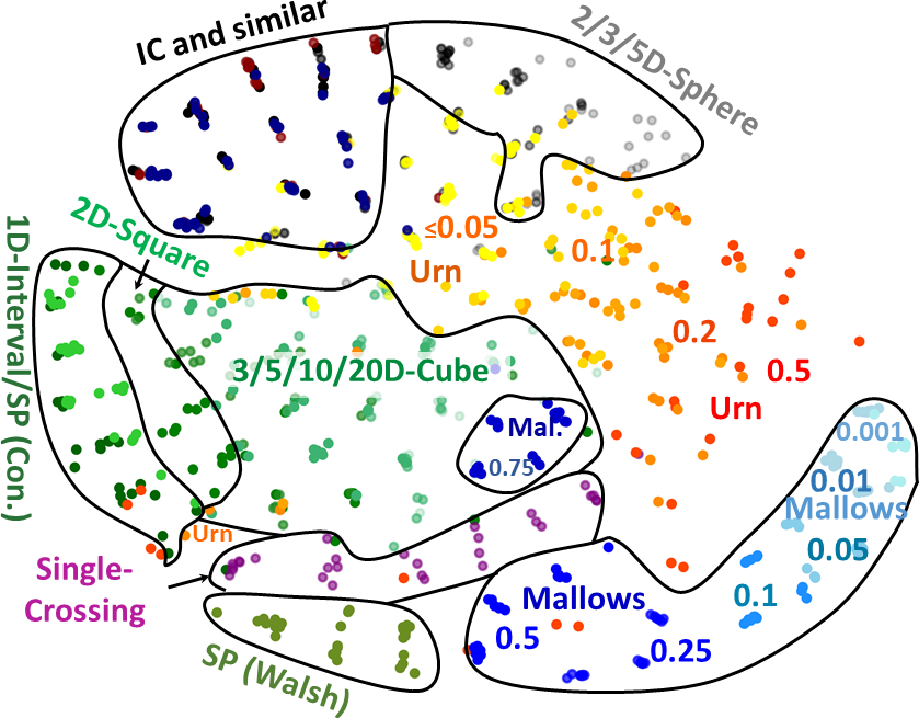
Figure 1: The map of elections, due to Szufa et al. [31]. Each point corresponds to an election and its color gives the model from which it came. Generally, the closer two points are, the more similar are the corresponding elections in their metric.

(a) Plurality

(b) Borda

Figure 2: Blue and red solid lines show the number of elections (on the $y$-axis) with a given $50\%$-winner threshold (on the $x$-axis) for Plurality and Borda, respectively. In the black scatter plots, each dot corresponds to an election. Its $x$-coordinate gives the $50\%$-winner threshold (perturbed, if many elections would overlap) and its $y$-coordinate gives the difference between the scores of the winner and the runner-up.

Computations. For each election $E$ and candidate $c$, let $P_{E,c}(r)$ be the probability that $c$ wins—under a given voting rule—in an election chosen uniformly at random from $R(E,r)$. Ideally, we would like to compute these values for all elections, candidates and swap distances, for Plurality and Borda. However, since #Swap-Bribery is $\#{\mathrm{P}}$-hard for both our rules, instead of computing these values exactly, we resorted to sampling. Specifically, for each election (except those with tied winners) and each normalized swap distance $r\in\{0.05,0.1,\ldots,1\}$ we sampled $500$ elections at this distance and for each candidate recorded the proportion of elections where he or she won (see Appendix B.2 for the sampling procedure). For each election, we quantified the robustness of its winner by identifying the smallest swap distance $r$, among the considered ones, for which he or she has winning probability below $50\%$. We refer to this value as the $50\%$-winner threshold (or, threshold, for short).

Results. In the following, we present several findings from our experiments, each followed by supporting arguments.

Finding 1.

The Borda winner of an election is usually more robust against random swaps than the Plurality winner.

The solid blue line in Figure 2(a) and the solid red line in Figure 2(b) show how many elections from our dataset have particular 50%-winner thresholds for Plurality and Borda, respectively. While for Borda the threshold of $0.45$ occurs far more often than the other ones, for Plurality, the distribution is more uniform (with small spikes at $0.1$ and $0.45$). So, Plurality elections are more likely to change results after relatively few swaps than the Borda ones. Two explanations are that (a) under Plurality there can be “strong contenders” who do not win, but who are often ranked close to the first place and, thus, can overtake the original winner after a few swaps, and (b) the Plurality winner has the highest chance of losing points, as he or she is ranked first most frequently. Under Borda, the candidates usually have similar chances of both gaining and losing a point with a single swap.

Finding 2.

The score difference between the winner and the runner-up (i.e., the candidate ranked in the second place) has a limitied predictive value for the $50\%$-winner threshold.

Let us consider the black scatter plots in Figures 2(a) (for Plurality) and 2(b) (for Borda). There, each election is represented as a dot, whose $x$-coordinate is the $50\%$-winner threshold (perturbed a bit if many elections were to take the same place) and whose $y$-coordinate is the score difference between the winner and the runner up. While there certainly is some correlation betwen these two values, the same score difference may lead to a wide range of $50\%$-winner thresholds (e.g., for Plurality a score difference of $10$ may lead to the threshold being anything between $0.1$ and $0.4$).

From now on, we focus on Plurality, but most of our conclusions also apply to Borda (we do mention some differences though; for details, see Appendix B.3). In Figure 3, we show the map of elections, with colors corresponding to each election’s $50\%$-winner threshold. The figure also includes six plots, each showing the values of $P_{E,c}(r)$ for four candidates in six selected elections (we discuss them later).

Figure 3: Map of elections visualizing the $50\%$-winner threshold for Plurality and six plots showing $P_{E,c}(r)$ as a functon of $r$, for six selected elections and the four most successful candidates in each (see the paragraph preceding 4 for details).

Finding 3.

Positions of elections on the map correlate with their $50\%$-winner thresholds. Elections sampled from the same model tend to have similar thresholds.

Consider the map in Figure 3. As we move from top to bottom and from left to right, the $50\%$-winner threshold tends to increase. Not surprisingly, it is low for IC elections (as they are completely random, it is natural that few changes can affect the result) and it is high for Mallows elections with low $\phi$ (most preference orders in these elections are identical, up to a few swaps). For urn elections, the threshold tends to increase with parameter $\alpha$ (as the votes become less varied with larger $\alpha$). Interestingly, the threshold is somewhat more varied among $t$D-Cube elections (as compared to the other models), and one can notice that for 1D-Interval elections it tends to be slightly lower than for higher-dimensional $t$D-Cube ones (this effect is much stronger for Borda). Yet, typically elections generated from a given model (with a given parameter) tend to have similar threshold values.

For further insights, we turn to the six plots in Figure 3. Each of them regards a particular election and four of its candidates. The candidates are marked with colors and the original winner is always red. For each considered election $E$ and each candidate $c$ in the plot, we show $P_{E,c}(r)$ for values of $r$ between $0$ and $0.5$ (specifically, for these six elections, we estimated $P_{E,c}(r)$ for $r\in\{0.0125,0.025,\ldots,0.5\}$ using 10’000 samples in each case). We limited the range of relative swap distances because above $0.5$, the votes are becoming similar to the reverses of the original ones. For each of the candidates, in the legend we provide his or her Plurality score, Borda score, and the rank in the original election (we use the Borda scores in further discussions). For each of the six elections, we sorted the candidates with respect to $\max_{r\in\{0,0.0125,\ldots,0.5\}}P_{E,c}(r)$ and chose the top four to be included in the plot. The elections were chosen to show interesting phenomena (thus the patterns they illustrate are not always the most common ones, but are not outliers either). The following discussion refines the observations from 2.

Finding 4.

Winners winning by a small margin are not necessarily close to losing. Winners winning by a large margin are robust but not necessarily very robust winners.

In Elections 1 to 4, the winners are very sensitive to random swaps: The blue candidate already wins a considerable proportion of elections even if only a $0.0125$ fraction of possible swaps are applied (i.e., about half a swap per vote, on average), and the red candidate quickly drops below $50\%$ winning probability. It is quite surprising that so few random swaps may change the outcome with fairly high probability. There are also differences among these four elections. For example, in Elections 1 and 2 the candidates have similar scores, but in Election 2 the red candidate stays the most probable winner until swap distance $0.4$, whereas in Election 1, the most probable winner changes quite early. The plots for Elections 3 and 4 are similar to that for Election 1, but come from tD-Cube elections of different dimension; this pattern appears in elections from other families of distributions too, but less commonly.

In Elections 1 to 4, the original winner has at most four Plurality points of advantage over the next candidate, so one could argue that scores suffice to identify close elections. Yet, in Election 5 the difference between the scores of the winner and the runner-up is $3$, but the red candidate stays a winner with probability greater than $50\%$ until swap distance $0.35$. Thus, looking only at the scores can be misleading. Nonetheless, if the score difference is large (say, above $25$), the $50\%$-winner threshold is always above $0.2$ (see Figure 2(a)). But, as witnessed in Election 6, even in such seemingly clear elections, around $10\%$ of random swaps suffice to change the outcome with a non-negligible probability.

Finding 5.

The score of a non-winning candidate has a limited predictive value for his or her probability of winning if some random swaps are performed.

Perhaps surprisingly, in some elections the most probable winner at some (moderately low) swap distance is not necessarily ranked highly in the original election. For instance, in Election 1 the green candidate is originally ranked seventh, but becomes the most probable winner already around swap distance $0.1$. Here, this can be explained by the fact that he or she has a significantly higher Borda score than the other candidates. So, he or she is ranked highly in many votes and can reach the top positions with only a few swaps. Yet, not all patterns can be explained this way. For example, in Elections 1 and 2, the first two candidates have similar Plurality and Borda scores but still behave quite differently, even at small swap distances.

5 Conclusions

We have shown that the counting variants of Swap-Bribery have high worst-case complexity, but, nonetheless, are very useful for analyzing the robustness of elections winners. In particular, we have observed some interesting phenomena, including the fact that the scores of the candidates do not suffice to evaluate their strengths. Establishing the complexity of Borda #Swap-Bribery parameterized by the swap radius remains as an intriguing open problem.

Acknowledgments. Niclas Boehmer was supported by the DFG project MaMu (NI 369/19). Piotr Faliszewski was supported by a Friedrich Wilhelm Bessel Award from the Alexander von Humboldt Foundation. Work started while all authors were with TU Berlin.

Appendix A Missing Proofs from Section 3

In this section, we provide missing details and proofs from Section 3.

A.1 Auxilary Algorithms

In this section we provide a number of polynomial-time algorithms for solving problems of the following form: Given an election and a particular budget (or, number of swaps) compute the number of ways of performing exactly this many swaps so that the election has some given shape (e.g., all the voters ranks the same given candidate on top). We refer to such problems as voter group contribution counting problems.

Swap Contribution for Plurality (Unit Prices)

Given an election $E=(C,V)$, a budget $r$, and a distinguished candidate $p\in C$, $\text{vgc}^{\text{Swap}}_{\text{Plurality}}(V,r,p)$ denotes the number of possibilities to perform exactly $r$ swaps so that $p$ is the top choice of every voter within $V$.

Lemma 7.

One can compute $\text{vgc}^{\text{Swap}}_{\text{Plurality}}(V,r,p)$ in time $O(n\cdot m^{4})$.

Proof.

Let $C=\{p,c_{2},\ldots,c_{m}\}$, $V=\{v_{1},\ldots,v_{n}\}$, $r$, and $p$ be given as described above. We define the following dynamic programming table $L$. An entry $L[i,r^{\prime}]$ denotes the number of possibilities to perform exactly $r^{\prime}$ swaps within the first $i$ votes in $V$ so that $p$ is the top choice for these $i$ voters.

Let $r^{*}(v)$ denote the number of swaps required to push candidate $p$ to the top position in vote $v$. We initialize the table via:

$$L[1,r^{\prime}]=\begin{cases}0&\text{if $r^{\prime}<r^{*}(v_{1})$}\\ Y(m-1,r^{\prime}-r^{*}(v_{1}))&\text{otherwise},\end{cases}$$

where $Y(m,k)$ denotes the number of permutations of swap distance $k$ from a given permutation with $m$ elements (algorithms for computing this value in polynomial time are well known). We update the table with increasing $i$ via

$$L[i,r^{\prime}]=\!\!\!\!\!\!\!\!\sum_{r^{*}(v_{i})\leq r^{\prime\prime}\leq r^{\prime}}\!\!\!\!\!\!\!\!Y(m-1,r^{\prime\prime}-r^{*}(v_{i}))\cdot L[i-1,r^{\prime}-r^{\prime\prime}].$$

Finally, $\text{vgc}^{\text{Swap}}_{\text{Plurality}}(V,r,p)=L[n,r]$ gives the solution.

The initialization is correct, because we have to push candidate $p$ to the top position at cost $r^{*}(v_{1})$. This fixes the first position and the other $m-1$ positions can be freely rearranged. Naturally, there are $Y(m-1,r^{\prime}-r^{*}(v_{1}))$ possibilities to do this. Similarly, in the update step we sum over all possibilities to distribute our $r^{\prime}$ swaps among the first $i-1$ votes and the $i$th vote (again, we need at least $r^{*}(v_{i})$ swaps to push $p$ to the top). In each case, the number of possibilities is the product of all possibilities to spend $r^{\prime\prime}$ for voter $i$ and $r^{\prime}-r^{\prime\prime}$ swaps for the first $i-1$ voters.

The table is of dimension $O(n\cdot m^{2})$. Computing each single table entry can be done in time $O(m^{2})$: Precomputing the table $Y$ with all entries takes $O(m^{2})$ time (see also Appendix B.2 where a recurrence is given) and with this being done, computing each single table entry of $L$ takes $O(m^{2})$ time since there are at most $m^{2}$ values for $r^{\prime\prime}$ and for each such value we have to do only a constant number of arithmetic operations. ∎

Shift Contribution for Plurality (Arbitrary Prices Encoded in Unary)

At first, let us consider the constructive variant of Shift-Bribery, where we can shift forward the preferred candidate $p$.

Let $E=(C,V)$ be an election where every voter prefers the same candidate $d\in C$. Let $r$ be a budget, $p\in C$ be a distinguished candidate, and $s$ be an integer score value. Moreover, we are given some cost function $c\colon(V,\mathbb{N})\rightarrow\mathbb{N}$ describing the costs $c(v,\ell)$ of shifting $p$ by $\ell$ positions forward. We define $\text{vgc}^{\text{Shift}+}_{\text{Plurality}}(V,r,p,s)$ as the number of possibilities to shift candidate $p$ forward at total costs $r$ within $V$ so that $p$ is ranked at the top position exactly $s$ times.

Lemma 8.

One can compute $\text{vgc}^{\text{Shift}+}_{\text{Plurality}}(V,r,p,s)$ in time $O(n^{2}\cdot r^{2})$.

Proof.

We assume that $V=\{v_{1},\ldots,v_{n}\}$ and compute $\text{vgc}^{\text{Shift}+}_{\text{Plurality}}$ using standard dynamic programming. Let $L[j,s^{\prime},r^{\prime}]$ be the number of ways to shift $p$ forward in the first $j$ votes in $V$ at total cost of $r^{\prime}$, so that $p$ obtains $s^{\prime}$ additional Plurality points.

We introduce two auxilliary functions, $\tau(v,x)$ and $\nu(v,x)$. Function $\nu(v,x)$ indicates whether spending cost $x$ for voter $v$ is valid (e.g., we cannot spend more than necessary to push $p$ to the top position) and function $\tau(v,x)$ indicates whether spending costs $x$ for voter $v$ is successful (i.e., pushes $p$ to the top position). Formally, we have:

$$\nu(v,x) =\begin{cases}1&\text{it is valid to spend cost~{}$x$ at voter~{}$v$,}\\ 0&\text{otherwise.}\end{cases}$$

$$\tau(v,x) =\begin{cases}1&\text{$p$ becomes top choice in~{}$v$ at cost~{}$x$,}\\ 0&\text{otherwise.}\end{cases}$$

We initialize our table with:

$$L[1,s^{\prime},r^{\prime}]=\begin{cases}\nu(v_{1},r^{\prime})\cdot\tau(v_{1},r^{\prime})&s^{\prime}=1\\ \nu(v_{1},r^{\prime})\cdot(1-\tau(v_{1},r^{\prime}))&s^{\prime}=0\\ 0&\text{otherwise.}\end{cases}\phantom{\text{123}}$$

We update $L[j,s^{\prime},r^{\prime}]$ for $j>1$ via $L[j,s^{\prime},r^{\prime}]=$

$$\sum_{r^{\prime\prime}\leq r^{\prime}}\big{(}L[j-1,s^{\prime}-1,r^{\prime\prime}]\cdot\tau(v_{j},r^{\prime}-r^{\prime\prime})\cdot\nu(v_{j},r^{\prime}-r^{\prime\prime})$$

$$+L[j-1,s^{\prime},r^{\prime\prime}]\cdot(1-\tau(v_{j},r^{\prime}-r^{\prime\prime}))\cdot\nu(v_{j},r^{\prime}-r^{\prime\prime})\big{)}.$$

The table $L$ is of size $n^{2}\cdot r$. Computing a single table entry requires at most $2r$ table lookups and at most $2r$ arithmetic operations. ∎

Let us now consider the destructive case, where we can push a given candidate backward. Consider an election $E=(C,V)$ with two distinguished candidates, $p$ and $d$, such that every voter either prefers $p$ the most while ranking candidate $d$ in the second position, or prefers $d$ the most. Let $r$ be the budget, and $s$ be an integer score value. Moreover, we are given some cost function $c\colon(V,\mathbb{N})\rightarrow\mathbb{N}$ describing the costs $c(v,\ell)$ of shifting $p$ by $\ell$ positions backward. We define $\text{vgc}^{\text{Shift}-}_{\text{Plurality}}(V,r,p,s)$ as the number of possibilities to shift candidate $p$ backward at total costs $r$ within $V$ such that $p$ is ranked exactly $s$ times at the top position.

Lemma 9.

One can compute $\text{vgc}^{\text{Shift}-}_{\text{Plurality}}(V,r,p,s)$ in time $O(n^{2}\cdot r^{3})$.

Proof.

We assume that $V=\{v_{1},\ldots,v_{n}\}$ and compute $\text{vgc}^{\text{Shift}-}_{\text{Plurality}}$using yet again standard dynamic programming, defining our table $L$ as follows. An entry $L[j,s^{\prime},r^{\prime}]$ contains the number of ways to shift $p$ backward in the first $j$ votes from $V$ at total cost of $r^{\prime}$, so that $p$ ends up with exactly $s^{\prime}$ points.

As in the constructive case, we introduce two auxilliary functions, $\tau(v,x)$ and $\nu(v,x)$. Function $\nu(v,x)$ indicates that spending cost $x$ for voter $v$ is valid and function $\tau(v,x)$ indicates that spending cost $x$ for voter $v$ is successful (pushes $d$ to the top position). Formally:

$$\nu(v,x) =\begin{cases}1&\text{it is valid to spend cost~{}$x$ at voter~{}$v$}\\ 0&\text{otherwise.}\end{cases}$$

$$\tau(v,x) =\begin{cases}1&\text{$d$ becomes top choice in~{}$v$ at cost~{}$x$}\\ 0&\text{otherwise.}\end{cases}$$

We initialize our table with:

$$L[1,s^{\prime},r^{\prime}]=\begin{cases}\nu(v_{1},r^{\prime})\cdot(1-\tau(v_{1},r^{\prime}))&s^{\prime}=1\\ \nu(v_{1},r^{\prime})\cdot\tau(v_{1},r^{\prime})&s^{\prime}=0\\ 0&\text{otherwise.}\end{cases}\phantom{\text{12}}$$

We update $L[j,s^{\prime},r^{\prime}]$ for $j>1$ via $L[j,s^{\prime},r^{\prime}]=$

$$\textstyle\sum_{r^{\prime\prime}\leq r^{\prime}}\big{(}L[j-1,s^{\prime},r^{\prime\prime}]\tau(v_{j},r^{\prime}-r^{\prime\prime})\nu(v_{j},r^{\prime}-r^{\prime\prime})$$

$$+L[j-1,s^{\prime}-1,r^{\prime\prime}](1-\tau(v_{j},r^{\prime}-r^{\prime\prime}))\nu(v_{j},r^{\prime}-r^{\prime\prime})\big{)}.$$

The table $L$ is of size $n^{2}\cdot r$. Computing a single table entry requires at most $2r$ table lookups and at most $2r$ arithmetic operations. ∎

A.2 Missing Details for the Proof of Theorem 2

For the proof of Theorem 2, we need to discuss how to compute the table $T$.

Lemma 10.

Table $T$ can be computed in time $O(n\cdot m^{7})$.

Proof.

We initialize the table by setting $T[1,1,r^{\prime}]=\text{vgc}^{\text{Swap}}_{\text{Plurality}}(V_{1},r^{\prime},p)$ and $T[1,\ell,r^{\prime}]=0$, $\forall\ell>1$. The table is filled with increasing $i$ by setting $T[i,\ell,r^{\prime}]$ to be:

$$\sum_{\ell^{\prime}<\ell,r^{\prime\prime}\leq r^{\prime}}(T[i-1,\ell^{\prime},r^{\prime\prime}]\cdot\text{vgc}^{\text{Swap}}_{\text{Plurality}}(V_{i},r^{\prime}-r^{\prime\prime},c_{\ell})).$$

Note that the initialization is correct by the definition of $\text{vgc}^{\text{Swap}}_{\text{Plurality}}(V,r,c)$ and the fact that the first group must consistently vote for $c_{1}=p$. For updating the table, we sum up over all possibilities to split the swap budget $r^{\prime}$ between the $i$th voter group and first $i-1$ voter groups, in combination with each possible candidate $c_{\ell^{\prime}}$ that may have been pushed to the top position by all voters of group $i-1$.

Computing table $T$ requires filling in $m\cdot m\cdot nm^{2}$ entries, and each entry takes $O(m^{3})$ time (due to the number of terms in the sum in the update step). All in all, the algorithm takes time $O(n\cdot m^{7})$, assuming that each of at most $m$ functions $\text{vgc}^{\text{Swap}}_{\text{Plurality}}$ was computed in time $O(n\cdot m^{4})$. ∎

A.3 Proof of Theorem 3

See 3

Proof.

In an instance of #Linear Extensions we are given a set $Z=\{z_{1},\ldots,z_{m}\}$ of items and a set $O\subseteq X\times X$ of constraints; we ask for the number of linear orders over $Z$ such that for each constraint $(x,y)\in O$, $x$ precedes $y$. We reduce this problem to Plurality #Swap-Bribery with $0/1$ prices (i.e., each swap either has a unit cost or is free) and budget $r:=0$ (if one preferred to avoid zero prices, then doing so would require only a few adaptations in the proof).

Given an instance of #Linear Extensions, as specified above, first we compute a single order $\succ$ that is consistent with the constraints (doing so is easy via standard topological sorting; if no such order exists, then we return zero and terminate). Next, we form an election $E$ with candidate set $C=\{p\}\uplus Z$ and a single vote $v$, where $p$ is ranked first and all the other candidates are ranked below, in the order provided by $\succ$. We set the swap prices so that:

1. For each candidate $z\in Z$, the price for swapping him or her with $p$ is one.

2. For each pair $(x,y)\in O$, the price for swapping $x$ and $y$ is one.

3. All other prices are zero.

We form an instance of Plurality #Swap-Bribery with this election, prices, and budget $r:=0$. We make a single query regarding this instance and output the obtained value.

To see that the reduction is correct, we notice that for every preference order that $v$ may have after performing swaps of price zero, it holds that (a) $p$ is ranked first (because swapping $p$ out of the first position has nonzero price) and (b) for all pairs $(x,y)\in O$, $x$ is ranked ahead of $y$ (because swapping $x$ and $y$ has nonzero cost). On the contrary, for every linear order $\succ^{\prime}$ that is consistent with $O$, it is possible to transform the preference order of $v$ so that $p$ is ranked first, followed by members of $Z$ in the order specified by $\succ^{\prime}$ (for each two candidates $x,y\in Z$ such that $x\succ y$ but $y\succ^{\prime}x$, the cost of swapping them is zero, and if we have not transformed our vote into the desired form yet, then there are always two such candidates that are ranked consecutively). ∎

A.4 Proof of Theorem 4

See 4

Proof for the constructive case.

A core observation for our algorithm is that, under #Shift-Bribery, every voter will either vote for $p$ (if we shift $p$ to the top position) or for its original top choice. This allows us to group the voters according to their top choices as follows. Let $(V_{0},V_{1},V_{2},\ldots,V_{m^{\prime}})$, where $m^{\prime}\leq m-1$, be a partition of voters into groups so that (in the original election) every two voters within each group $V_{i}$ share the same top choice, while every two voters from different groups have different top choices; additionally, we require that the voters in group $V_{0}$ rank the distinguished candidate $p$ on the top position.

For each candidate $c$, let $s(c)$ be the original score of $c$. The idea of our algorithm is to count, for each possible final score $s^{*}\geq s(p)$ of $p$, the number of ways to spend the given budget $r$, so that $p$ obtains $s^{*}$ points while no other candidate obtains more than $s^{*}$ points. For each possible $s^{*}$ we create one global dynamic programming table $T_{s^{*}}$.

Our global tables are defined as follows. An entry $T_{s^{*}}[i,s^{\prime},r^{\prime}]$ contains the number of ways to shift $p$ forward in the voter groups $V_{1},\ldots,V_{i}$ at total cost of $r^{\prime}$, so that $p$ obtains $s^{\prime}$ additional points while no top choice from any voter group $V_{1},\ldots,V_{i}$ receives more than $s^{*}$ points.

To compute the values in table $T$, we will use the following local counting problem, maintaining the voter group contribution: Given a voter group $V^{\prime}$, a budget $r^{\prime}$, a distinguished candidate $p$, and a score $s^{\prime}$, compute the number of possibilities $\text{vgc}^{\text{Shift}+}_{\text{Plurality}}(V^{\prime},r^{\prime},p,s^{\prime})$ to shift candidate $p$ by in total $r^{\prime}$ positions within $V^{\prime}$, so that $p$ is ranked exactly $s^{\prime}$ times at the top position. This number can be computed in polynomial time (see Lemma 8 in Appendix A.1).

The intitialization of $T_{s^{*}}$ is straight-forward, by setting:

$$T_{s^{*}}[1,s^{\prime},r^{\prime}]=\text{vgc}^{\text{Shift}+}_{\text{Plurality}}(V_{1},r^{\prime},p,s^{\prime})$$

when $|V_{1}|-s^{\prime}\leq s^{*}$, and by setting $T_{s^{*}}[1,s^{\prime},r^{\prime}]=0$ when $|V_{1}|-s^{\prime}>s^{*}$ (the condition $|V_{1}|-s^{\prime}\leq s^{*}$ is to ensure that the top-ranked candidate of the voters from group $V_{1}$ obtains no more than $s^{*}$ points). We update the tables for $i>1$ by setting $T_{s^{*}}[i,s^{\prime},r^{\prime}]$ to be:

$$\textstyle\sum_{s^{\prime\prime}=|V_{i}|-s^{*}}^{s^{\prime}}\sum_{r^{\prime\prime}\leq r^{\prime}}\big{(} T_{s^{*}}[i-1,s^{\prime}-s^{\prime\prime},r^{\prime}-r^{\prime\prime}]\cdot\text{vgc}^{\text{Shift}+}_{\text{Plurality}}(V_{i},r^{\prime\prime},p,s^{\prime\prime})\big{)}.$$

(Again, the lower bound on $s^{\prime\prime}$ ensures that the candidate the voters from group $V_{i}$ vote for (if not $p$) obtains no more than $s^{*}$ points.) It is not hard to see that this indeed computes the values in the table correctly, without double-counting.

Assuming $\text{vgc}^{\text{Shift}+}_{\text{Plurality}}$ and global tables are computed correctly, it is not hard to verify that the overall solution is:

$$\sum_{s^{*}:=s(p)}^{s(p)+r}T_{s^{*}}[m^{\prime},s^{*}-s(p),r].$$

Indeed, between two different “guesses” of the final score $s^{*}$, double-counting is impossible. ∎

Proof for the destructive case.

The main ideas behind the destructive case are very similar to those behind the constructive one. The core observation is that under destructive Plurality #Shift-Bribery every voter will either vote for the distinguished candidate $p$ (if $p$ is the voter’s top choice and is not shifted backward) or for some other candidate $d\neq p$ (either if $p$ were not the voter’s top choice but $d$ were, or if $p$ were the top choice but was shifted backward so that $d$, which was originally in the second position, was moved to the top). In either case, we call candidate $d$ the non-$p$ choice of voter $v$. This allows us to group all voters according to their non-$p$ choices as follows. Let $(V_{1},V_{2},\ldots,V_{m^{\prime}}),m^{\prime}\leq m$, be a partition of voters into groups $V_{i}$ such that every two voters within the same group $V_{i}$ have the same non-$p$ choice while every two voters from different groups have different non-$p$ choices.

Let $s(c)$ be the original score of candidate $c$. The idea of our algorithm is to count, for each possible final score $s^{*}\leq s(p)$ of $p$ the number of ways to spend the given budget $r$ so that $p$ obtains $s^{*}$ points while at least one other candidate obtains more than $s^{*}$ points. For each possible $s^{*}$ we create one global dynamic programming table $T_{s^{*}}$.

Our global tables are defined as follows. An entry $T_{s^{*}}[i,s^{\prime},r^{\prime},\text{false}]$ contains the number of ways to shift $p$ backward in the voter groups $V_{1},\ldots,V_{i}$ at total cost of $r^{\prime}$, so that $p$ obtains $s^{\prime}$ points from $V_{1},\ldots,V_{i}$ while no non-$p$ choice of any voter group $V_{1},\ldots,V_{i}$ receives more than $s^{*}$ points. An entry $T_{s^{*}}[i,s^{\prime},r^{\prime},\text{true}]$ contains the number of ways to shift $p$ backward in the voter groups $V_{1},\ldots,V_{i}$ at total cost of $r^{\prime}$, so that $p$ obtains $s^{\prime}$ points from $V_{1},\ldots,V_{i}$ while a non-$p$ choice of at least one voter group from $V_{1},\ldots,V_{i}$ receives more than $s^{*}$ points.

To compute the entries of the table $T$, we will use the following local counting problem maintaining the voter group contribution: Given a voter group $V^{\prime}$, a budget $r^{\prime}$, a distinguished candidate $p$, and a score $s^{\prime}$, compute the number $\text{vgc}^{\text{Shift}-}_{\text{Plurality}}(V^{\prime},r^{\prime},p,s^{\prime})$ of possibilities to shift candidate $p$ backward at total costs $r^{\prime}$ within $V^{\prime}$, so that $p$ is ranked exactly $s^{\prime}$ times at the top position. This number can be computed in polynomial time (see Lemma 9 in Appendix A.1).

The intitialization of $T_{s^{*}}$ is as follows:

1. If $|V_{1}|-s^{\prime}\leq s^{*}$, then

   $$T_{s^{*}}[1,s^{\prime},r^{\prime},\text{false}]=\text{vgc}^{\text{Shift}-}_{\text{Plurality}}(V_{1},r^{\prime},p,s^{\prime}),$$

   and otherwise $T_{s^{*}}[1,s^{\prime},r^{\prime},\text{false}]=0$.

2. If $|V_{1}|-s^{\prime}>s^{*}$ then

   $$T_{s^{*}}[1,s^{\prime},r^{\prime},\text{true}]=\text{vgc}^{\text{Shift}-}_{\text{Plurality}}(V_{1},r^{\prime},p,s^{\prime}),$$

   and otherwise $T_{s^{*}}[1,s^{\prime},r^{\prime},\text{true}]=0$.

We compute the table entries for $i>1$ as follows. We set $T_{s^{*}}[i,s^{\prime},r^{\prime},\text{false}]$ to be

$$\textstyle\sum_{s^{\prime\prime}=|V_{i}|-s^{*}}^{s^{\prime}}\sum_{r^{\prime\prime}\leq r^{\prime}}\big{(}T_{s^{*}}[i-1,s^{\prime}-s^{\prime\prime},r^{\prime}-r^{\prime\prime},\text{false}]\cdot\text{vgc}^{\text{Shift}-}_{\text{Plurality}}(V_{i},r^{\prime\prime},p,s^{\prime\prime})\big{)}.$$

(The lower bound on $s^{\prime\prime}$ ensures that the non-$p$ choice obtains no more than $s^{*}$ points.) And we set $T_{s^{*}}[i,s^{\prime},r^{\prime},\text{true}]$ to be:

$$\sum_{\begin{subarray}{c}s^{\prime\prime}\leq s^{\prime},|V_{i}|-s^{\prime\prime}>s^{*}\end{subarray}}\sum_{r^{\prime\prime}\leq r^{\prime}}(T_{s^{*}}[i-1,s^{\prime}-s^{\prime\prime},r^{\prime}-r^{\prime\prime},\text{false}]\cdot\text{vgc}^{\text{Shift}-}_{\text{Plurality}}(V_{i},r^{\prime\prime},p,s^{\prime\prime}))$$

$$+\sum_{\begin{subarray}{c}s^{\prime\prime}\leq s^{\prime}\end{subarray}}\sum_{r^{\prime\prime}\leq r^{\prime}}(T_{s^{*}}[i-1,s^{\prime}-s^{\prime\prime},r^{\prime}-r^{\prime\prime},\text{true}]\cdot\text{vgc}^{\text{Shift}-}_{\text{Plurality}}(V_{i},r^{\prime\prime},p,s^{\prime\prime}))$$

The first two sums account for the case that the non-$p$ choice of group $V_{i}$ is the first candidate non-$p$ candidate to obtain more than $s^{*}$ points. The second two sums account for the case where already some non-$p$ choice of some previous group obtained more than $s^{*}$ points. One can verify that this indeed computes the table correctly without double-counting.

Assuming $\text{vgc}^{\text{Shift}-}_{\text{Plurality}}$ and global tables are computed correctly, it is not hard to verify the the overall solution is:

$$\sum_{s^{*}:=s(p)-r}^{s(p)}T_{s^{*}}[m^{\prime},s^{*},r,\text{true}].$$

Indeed, between two different “guesses” of the final score $s^{*}$, double-counting is impossible. ∎

A.5 Proof of Theorem 5

See 5

Proof.

For the constructive case, it suffices to follow the proof of Bredereck et al. [6]. For the destructive case, we give a Turing reduction from the #Multicolored Independent Set problem, which is well-known to be $\#{\mathsf{W[1]}}$-complete (indeed, #Independent Set is equivalent to #Clique, which is a canonical $\#{\mathsf{W[1]}}$-complete problem; the multicolored variants of these problem remain $\#{\mathsf{W[1]}}$-complete).

Let $I=(G,h)$ be an instance of #Multicolored Independent Set, where $G=(V(G),E(G))$ is a graph where each vertex has one of $h$ colors; we ask for the number of size-$h$ independent sets (i.e., sets of vertices such that no two vertices have a common edge) such that each vertex has a different color. Without loss of generality, we assume that there are no edges between vertices of the same color and that the number of vertices of each color is the same, denoted by $n$. For each color $\ell\in[h]$, let $V(\ell):=\{v^{\ell}_{1},\ldots,v^{\ell}_{n}\}$ denote the set of vertices with color $\ell$. For each vertex $v^{\ell}_{i}\in V(G)$, let $E(v^{\ell}_{i})$ denote the set of edges incident to this vertex. Finally, let $\Delta:=\max_{v\in V(G)}|E(v)|$ be the highest degree of a vertex in $G$.

Our reduction proceeds as follows. Let $r:=h(n(\Delta+1)+\Delta)$ be our shift radius. We form an election with the following candidates. First, we add a candidate $d$, who will be the original winner of the election, and we treat sets $V(G)$ and $E(G)$ as sets of vertex and edge candidates. For each vertex $v^{\ell}_{i}\in V(G)$, we form a set $F(v^{\ell}_{i})$ of $\Delta-|E(v^{\ell}_{i})|$ fake-edge candidates, so we will be able to pretend that all vertices have the same degree; we write $F(G)$ to denote the set of all fake-edge candidates. Next, we form a blocker candidate $b$ and a set $B$ of $r$ additional blocker candidates, whose purpose will be to limit the extent to which we can shift $d$ in particular votes. Finally, we let $X=\{x_{1},\ldots,x_{5}\}$ be a set of five candidates that we will use to fine-tune the scores of the other candidates. Altogether, the candidate set is:

$$C:=\{d\}\uplus V(G)\uplus E(G)\uplus F(G)\uplus B\uplus\{b\}\uplus X.$$

For each vertex $v^{\ell}_{i}$, by $H(v^{\ell}_{i})$ we mean the (sub)preference order where $v^{\ell}_{i}$ is ranked on top and is followed by the candidates from $E(v^{\ell}_{i})\uplus F(v^{\ell}_{i})$ in some arbitrary order. We write $\overleftarrow{H(v^{\ell}_{i})}$ to denote the corresponding reverse order. We form the following $4h+2$ voters:

1. For each color $\ell\in[h]$, we introduce voters $e(\ell)$ and $f(\ell)$ with preference orders:

   $$\!\!\!e(\ell)\colon b\succ d\succ H(v^{\ell}_{1})\succ\cdots\succ H(v^{\ell}_{n})\succ B\succ X,$$

   $$f(\ell)\colon b\succ d\succ\overleftarrow{H(v^{\ell}_{n})}\succ\cdots\succ\overleftarrow{H(v^{\ell}_{1})}\succ B\succ X.$$

   We also introduce voters $e^{\prime}(\ell)$ and $f^{\prime}(\ell)$, whose preference orders are obtained by reversing those of $e(\ell)$ and $f(\ell)$, respectively, and shifting the candidates from $X$ to the back (the exact order of the candidates from $X$ in the last five positions is irrelevant).

2. Let $\sigma$ be the following preference order:

   $$\sigma\colon V(G)\succ x_{1}\succ E(G)\succ F(G)\succ x_{2}\succ x_{3}\succ x_{4}\succ x_{5}\succ B\succ d\succ b.$$

   We introduce four voters, $s_{1},s_{2},s_{3},s_{4}$. Voter $s_{1}$ has preference order $\sigma$, except that members of $B$ are shifted ahead of $x_{5}$, and voter $s_{2}$ has the preference order obtained from $\sigma$ by (a) shifting $x_{1}$ to the top, (b) shifting $x_{2}$, $x_{3}$, and $x_{4}$ ahead of the candidates from $E(G)\uplus F(G)$, and (c) shifting $d$ ahead of $B$. Voters $s_{3}$ and $s_{4}$ have preference orders that are reverses of $\sigma$.

Let $E$ be the just-constructed election. If $s_{1}$ and $s_{2}$ had preference order $\sigma$, then all candidates, except those in $X$, would have the same score (because for each voter there would be a matching one, with the same preference order but reversed, except that both voters might rank members of $X$ on the bottom); let this score be $L$. Due to the changes in $s_{1}$’s and $s_{2}$’s preference orders:

1. candidate $d$ has score $L+r$,

2. every vertex candidate has score $L-1$,

3. every edge and fake-edge candidate has score $L-3$,

4. every blocker candidate has score $L$, and

5. every candidate in $X$ has score much below $L-r$.

Let $I^{\prime}$ be an instance of Borda #Destructive Shift-Bribery with election $E$, designated candidate $d$, and shift radius $r$. Further, let $M$ be the set of elections that can be obtained from $E$ by shifting $d$ back by $r$ positions in total, let $f(I)$ be the number of solutions for $I$ (i.e., the number of multicolored independent sets of size $h$ in $G$), and let $g(I^{\prime})$ be the number of solutions for $I^{\prime}$ (i.e., the number of elections in $M$ where $d$ is not a winner). We claim that $f(I)=|M|-g(I^{\prime})$. In other words, we claim that each election where $d$ wins and which can be obtained from $E$ by shifting him or her back by $r$ positions in total, corresponds to a unique multicolored independent set in $G$. Since $|M|$ can be computed in polynomial time using a simple dynamic program, showing that our claim holds will complete the proof. First, in Step 1, we show that each solution for $I$ corresponds to a unique election from $M$ where $d$ wins (and which is obtained by shifting $d$ by $r$ positions back), and then, in Step 2, we show that the reverse implication holds.

Step 1.

Let $S=\{v^{1}_{i_{1}},\ldots,v^{h}_{i_{h}}\}$ be some multicolored independent set of $G$. We obtain a corresponding solution for $I^{\prime}$ as follows: For each $\ell\in[h]$, we shift $d$ in $e(\ell)$ to be right in front of $v^{\ell}_{i_{\ell}+1}$ (or, to be right in front of the first blocker candidate, if $i_{\ell}=n$), and we shift $d$ in $f(\ell)$ to be right in front of $v^{\ell}_{i_{\ell}}$. Doing so requires $n(\Delta+1)+\Delta$ unit shifts for each $\ell\in[h]$, so , altogether, we make $r=h(n(\Delta+1)+\Delta)$ unit shifts. As a consequence, $d$ has score $L$ and every other candidate has score at most $L$. Indeed, $d$ passes each vertex candidate exactly once, and each edge and fake-edge candidate at most three times. The former is readily verifiable. The latter can be seen as follows: Fix a color $\ell\in[h]$ and consider voters $e(\ell)$ and $f(\ell)$. In their preference orders, $d$ passes each edge candidate incident to a vertex in $V(\ell)\setminus\{v^{\ell}_{i_{\ell}}\}$ exactly once (either in $e(\ell)$ or in $f(\ell)$), and $d$ passes each edge candidate incident to $v^{\ell}_{i_{\ell}}$ exactly twice (once in $e(\ell)$ and once in $f(\ell)$). Thus, each edge candidate is passed by $d$ at most three times (if neither of its endpoints is in $S$, then it is passed twice, and if one of its endpoints is in $S$, then it is passed three times; both of its endpoints cannot belong to $S$ by definition of an independent set). Similarly, $d$ passes each fake-edge candidate at most three times. Finally, $d$ never passes any of the blocker candidates. Thus, $d$ is a winner in the resulting election.

Step 2.

For the other direction, consider an election $E^{\prime}$ obtained from $E$ by shifting $d$ backward by $r$ positions in total, where $d$ still is a winner. We will show that $E^{\prime}$ corresponds to a unique, size-$h$, multicolored independent set in $G$. First, we recall that $d$ has score $L$ in $E^{\prime}$ (this is so because he or she had score $L+r$ in $E$ and was shifted by $r$ positions backward). This means that to remain a winner, $d$ could not have passed any of the blocker candidates, because then some blocker candidate would have more than $L$ points. As a consequence, the only votes in which $d$ could have been shifted are $e(\ell)$ and $f(\ell)$, for each $\ell\in[h]$. Further, in each of these votes $d$ could have been shifted by at most $n(\Delta+1)$ positions. In fact, it must have been the case that for each $\ell\in[h]$, the total number of positions by which $d$ was shifted in $e(\ell)$ and $f(\ell)$ was exactly $r/h=n(\Delta+1)+\Delta$. If this were not the case, then for some $\ell$, candidate $d$ would have been shifted by more than $n(\Delta+1)+\Delta$ positions in total in $e(\ell)$ and $f(\ell)$ and, as a consequence, $d$ would have passed at least one vertex candidate from $V(\ell)$ twice. Such a vertex candidate would end up with score at least $L+1$ and $d$ would not have been a winner. To convince oneself that this is the case, let $y$ be some positive integer and consider vote $e(\ell)$ with $d$ shifted by $n(\Delta+1)$ positions to the back (right in front of the first blocker candidate), and vote $f(\ell)$ with $d$ shifted by $\Delta+y$ positions to the back. Initially $d$ passes $v^{\ell}_{n}$ in both $e(\ell)$ and $f(\ell)$. Now consider the process of repeatedly undoing a single unit shift in $e(\ell)$ and performing a single additional unit shift in $f(\ell)$. At each point of this process, there is at least one vertex candidate in $V(\ell)$ such that $d$ is ranked behind this vertex in both votes.

Analogous reasoning shows that for each $\ell\in[h]$, there is a number $i_{\ell}\in[n]$ such that in $e(\ell)$ candidate $d$ is shifted back by exactly $i_{\ell}(\Delta+1)$ positions, and in $f(\ell)$ candidate $d$ is shifted back by $(n-i_{\ell})(\Delta+1)+\Delta$ positions (indeed, it suffices to repeat the reasoning from the end of the above paragraph for $y=0$ to see that these are the only numbers of shifts for which $d$ never passes any of the candidates from $V(\ell)$ twice). Now we note that the set $S:=\{v^{1}_{i_{1}},\ldots,v^{h}_{i_{h}}\}$ is a size-$h$, multicolored, independent set: The first two observations are immediate; for the latter, we note that—analogously to the reasoning in Step 1—if $S$ were not an independent set, then $d$ would pass some edge candidate four times, giving him or her score $L+1$, which would prevent $d$ from being a winner. ∎

A.6 Proof of Theorem 6

See 6

Proof (constructive case).

We show how Borda #Constructive Shift-Bribery parameterized by the radius $r$ can be solved in ${\mathrm{FPT}}$ time using dynamic programming. We start with the assumption of unit costs and later explain how to extend the dynamic program to work with arbitrary unary-encoded costs.

First, observe that, given some budget $r$ and unit costs, we know the final score $s^{*}$of candidate $p$ after shifting it foward by $r$ position in total ($p$ gains one point with each position it is shifted forward). Our problem becomes very easy when every other candidate already has score at most $s^{*}$(before shifting $p$), because clearly no candidate other than $p$ may gain a point.

In general, since other candidates loose $r$ points in total, there may be up to $r$ critical candidates that have score greater than $s^{*}$(before shifting $p$). Moreover, for each critical candidate $c$ we can compute a demand value $d(c)$ which denotes the number of times $p$ must get shifted ahead of $c$ (equivalently, $d(c)$ is the original score of $c$ minus $s^{*}$).

Let the candidate set be $C=\{p,c_{1},\ldots,c_{m}\}$ and, for the ease of presentation, assume that the candidates $c_{1},\ldots,c_{m}$ are sorted by their demand values (with non-critical candidates having demand zero). We define the initial demand vector $\vec{d_{0}}$ to be an $r$-dimensional vector of natural numbers where the $i$-th component $\vec{d}[i]$ specifies how many times candidate $p$ needs to pass candidate $c_{i}$ to ensure that $c_{i}$ has at most score $s^{*}$ (if $r$ is larger than the number of non-$p$ candidates, we pad the demand vector with zeros; for simplicity, in the further discussion we assume that $r$ is at most as larger as the number of non-$p$ candidates). Thus we have $\vec{d}_{0}=(d(c_{1}),\ldots,d(c_{r}))$.

For each voter $v$ and non-negative integer $r^{\prime}\leq r$ we define the gain vector as

$${\vec{g}(v,r^{\prime})}=(g(c_{1},v,r^{\prime})\ldots,g(c_{r},v,r^{\prime})),$$

where $g(c_{i},v,r^{\prime})=1$ if $p$ passes candidate $c_{i}$ when $p$ is shifted forward at cost $r^{\prime}$ in vote $v$. If spending cost $r^{\prime}$ in vote $v$ is impossible (e.g., because $p$ would already be pushed to the top position at a lower cost), then we set the gain vector to $(-2r,\ldots,-2r)$. This way, we later ensure that such “invalid actions” are never counted. Naturally, given some voter $v$ and some non-negative integer $r^{\prime}\leq r$, the vector $\vec{d}^{\prime}=\vec{d}_{0}-\vec{g}(v,r^{\prime})$ describes the demand vector assuming that $p$ was shifted forward by $r^{\prime}$ position in vote $v$. Note that there are at most $(r+1)^{\min(r,m)}$ possible demand vectors.

We are now ready to solve our problem via dynamic programming, using table $T$ of ${\mathrm{FPT}}(r)$ size. More precisely, let $T[i,r^{\prime},\vec{d}]$ denote the number of ways to shift $p$ by $r^{\prime}$ positions in total, within the first $i$ voters, and ending up with demand vector $\vec{d}$. The overall solution for our problem will be in the entry $T[n,r,\vec{0}]$. It remains to show how to compute the entries of $T$.

We do so with increasing $i$, going over all combinations of $r^{\prime}$ and $\vec{d}$. Clearly, $T[1,\dots]$ has to be initialized mostly with zero entries since at most $r$ different demand vectors can be realized. More precisely, we have:

$$T[1,r^{\prime},\vec{d}]=\begin{cases}1&\text{if }\vec{d}=\vec{d}_{0}-\vec{g}(v_{1},r^{\prime})\\ 0&\text{otherwise}.\end{cases}$$

We fill-in the table for each $i>1$ using formula:

$$T[i,r^{\prime},\vec{d}]=\sum_{\begin{subarray}{c}r^{\prime\prime}\leq r^{\prime},\\ \vec{d}^{\prime}\leq^{1}\vec{d}\end{subarray}}T[i-1,r^{\prime}-r^{\prime\prime},\vec{d}^{\prime}]\cdot{[\vec{d}=(\vec{d}^{\prime}-g(v_{i},r^{\prime\prime}))]},$$

where $\vec{d}^{\prime}\leq^{1}\vec{d}$ holds if vector $\vec{d}^{\prime}$ is component-wise equal or smaller by at most one compared to $\vec{d}$ (formally, $\vec{d}^{\prime}\leq^{1}\vec{d}\Leftrightarrow\forall j\in[r]:\vec{d}[j]-1\leq\vec{d}^{\prime}[j]\leq\vec{d}[j]$), and where $[[X]]$ is one if equation $X$ holds and zero otherwise. Note that this recurrence goes over all possible ways to distribute the budget $r^{\prime}$ among the first $i-1$ voters and voter $v_{i}$, while only considering demand vectors that can be reached with the respective budget for voter $v_{i}$.

The table size is upper-bounded by $n\cdot r\cdot(r+1)^{\min(r,m)}$. Initializing a table entry works in $O(m)$ time (compute the gain vector and compare the demand vectors). While updating the table, an entry can be computed in time $r\cdot 2^{\min(r,m)}\cdot O(m)$ because there are at most $r$ possibilities for $r^{\prime\prime}$ and at most $2^{\min(r,m)}$ possibilities for $\vec{d}^{\prime}$. Altogether, this means we can compute $T$ and solve our problem in ${\mathrm{FPT}}$ time with respect to the shift radius $r$.

Finally, we explain how to extend the ${\mathrm{FPT}}$-algorithm to also work with arbitrary unarily encoded costs. The crucial difference for non-unit costs is that we cannot compute the final score of $p$ from our budget $r$. Instead, we guess (that is, go through all possibilities) the final score and then apply the algorithm described above with small modifications. To ensure that $p$ indeed ends up with the desired final score, we have to keep track of the score $p$ obtains. This can easily be done by extending the demand (resp. gain) vector by one more component that stores the number of times $p$ has to pass (resp. passes) some candidate. ∎

Proof (destructive case).

The proof is provided in the main body of the paper. ∎

Appendix B Additional Material for Section 4

B.1 Statistical Cultures

Here we briefly recall the four statistical cultures that we mention in our experimental studies:

Impartial Culture.

In the impartial culture model (IC), each election consists of preference orders chosen uniformly at random.

The Urn Model.

In the urn model, with parameter $\alpha\in\mathbb{R_{+}}$, to generate an election (with $m$ candidates), we start with an urn containing all $m!$ preference orders and generate the votes one by one, each time drawing the vote from the urn and then returning it there with $\alpha m!$ copies.

The Mallows Model.

In the Mallows model, with parameter $\phi\in[0,1]$, each election has a central preference order $v^{*}$ (chosen uniformly at random) and the votes are sampled from a distribution where the probability of obtaining vote $v$ is proportional to $\phi^{d_{\text{swap}}(v^{*},v)}$.

Euclidean Models.

In the $t$D-Cube and $t$D-Sphere models, the candidates and voters are points sampled uniformly at random from a $t$-dimensional hypercube/sphere, and the voters rank the candidates with respect to their distance (so a voter ranks the candidate whose point is closest to that of the voter first, then the next closest candidate, and so on).

Additionally, we also briefly describe the other models that are included in the dataset of Szufa et al. [31].

Single-Peaked Elections. Let $C=\{c_{1},\ldots,c_{m}\}$ be a set of candidates and let $\lhd$ be a linear order over $C$. We will refer to $\lhd$ as the societal axis. We say that a voter $v$’s preference order is single-peaked with respect to the axis if for every $t\in[m]$ it holds that $v$’s $t$ top-ranked candidates form an interval within $\lhd$. An election $E=(C,V)$ is single-peaked with respect to a given axis if each voter’s preference order is single-peaked with respect to this axis; an election is single-peaked if it is single-peaked with respect to some axis.

The notion of single-peakedness is due to Black [5] and is intuitively understood as follows: The societal axis orders the candidates with respect to positions on some one-dimensional issue (e.g., it may be the level of taxation that the candidate support, or a position on the political left-to-right spectrum). Each voter cares only about the issue represented on the axis. So, each voter chooses his or her top-ranked candidate freely, but then the voter chooses the second-best one among the two candidates next to the favorite one on the axis, and so on.

Szufa et al. [31] use the following two models for generating single-peaked elections (in both models, the societal axis is chosen uniformly at random and the votes are generated one-by-one, until a required number is produced):

Single-Peaked (Conitzer).

In the Conitzer model, we generate a vote as follows. First, we choose the top-ranked candidate uniformly at random. Then, we perform $m-1$ iterations, extending the vote with one candidate in each iteration: With probability $\nicefrac{{1}}{{2}}$ we extend the vote with the candidate “to the left” of the so-far ranked ones, and with probability $\nicefrac{{1}}{{2}}$ we extend it with the one “to the right” of the so-far ranked ones (if we ran out of the candidates on either side, then, naturally, we always choose the candidate from the other one). This model was popularized by Conitzer [12] and, hence, its name.

Single-Peaked (Walsh).

In the Walsh model, we generate votes by choosing them uniformly at random from the set of all preference orders single-peaked with respect to a given axis. This model was popularized by Walsh [33], who also provided a sampling algorithm.

Szufa et al. [31] give a detailed analysis explaining why these two models produce quite different elections (they also point out that 1D-Interval elections tend to be very similar to single-peaked elections from the Conitzer model).

Elecitons Single-Peaked on a Circle (SPOC). Peters and Lackner [29] extended the notion of single-peaked elections to single-peakedness on a circle. The model is very similar to the classic notion of single-peakedness, except that the axis is cyclic. Let $C$ be a set of $m$ candidates. Voter $v$ has a preference order that is single-peaked on a circle with respect to the axis $\lhd$ if for every $t\in[m]$ it holds that the set of $t$ top-ranked candidates according to $v$ either forms an interval with respect to $\lhd$ or a complement of an interval.

Szufa et al. [31] generate SPOC elections in the same way as single-peaked elections in Conitzer’s model, except that the axis is cyclic (so one never “runs out of candidates” on one side). Such SPOC elections are quite similar to 2D-Hypersphere ones (and, as indicated by Szufa et al., also to IC elections).

Single-Crossing Elections. Intuitively, an election is single-crossing if it is possible to order the voters so that for each two candidates $a$ and $b$, as we consider the voters in this order, the relative ranking of $a$ and $b$ changes at most once. Formally, single-crossing elections are defined as follows.

Let $E=(C,V)$ be an election, where $C=\{c_{1},\ldots,c_{m}\}$ and $V=(v_{1},\ldots,v_{n})$. This election is single-crossing with respect to its natural voter order if for each two candidates $c_{i}$, $c_{j}$ there is an integer $t_{i,j}$ such that the set $\{\ell\mid v_{\ell}$ ranks $c_{i}$ above $c_{j}\}$ is either $\{1,2,\ldots,t_{i,j}\}$ or $\{t_{i,j},\ldots,n-1,n\}$. An election is single-crossing if it is possible to reorder its voters so that it becomes single-crossing with respect to the natural voter order.

It is not clear how to generate single-crossing elections uniformly at random, or what a good procedure for generating single-crossing elections should be. Szufa et al. [31] propose one procedure and we point the reader to their paper for the details.

B.2 Sampling Elections

In our experiments, to calculate $P_{E^{\prime},c}(r)$ for different candidates $c$, elections $E^{\prime}$, and swap distances $r$, we sampled elections at swap distance $r$ from $E^{\prime}$ uniformly at random. Unfortunately, to achieve this, it is not enough to simply perform $r$ swaps in some of the votes in $E^{\prime}$, as this procedure does not necessarily produce an election at distance $r$ and cannot be easily adapted to result in a uniform distribution. Thus, we use a sampling procedure that relies on counting the number of elections at some swap distance $r$.

To compute this value, we employ dynamic programming using a table $T^{m}_{E}$: Each entry $T^{m}_{E}[n,r]$ contains the number of elections at swap distance $r$ from a given fixed election with $n$ voters and $m$ candidates (note that it is irrelevant what this election is, so we can simply assume an election with $n$ identical votes). In the following, let $u(m)=\frac{m(m-1)}{2}$ denote the maximal number of swaps that can be performed in a vote.

To compute $T^{m}_{E}$, we start by computing $T^{m}_{E}[1,r]$, that is, the number of votes at swap distance $r$ from a given single vote over $m$ candidates. We compute this value using dynamic programming. As we will use this quantity separately in the following sampling algorithm, we create a separate table $T_{V}$ for it, where $T_{V}[m,r]$ contains the number of votes at swap distance $r$ from a given vote over $m$ candidates. Note that $T_{V}[m,r]$ is simply the number of permutations over $m$ elements with $r$ inversions. Computing this value is a well-studied problem and we use the following procedure [28]: We initialize the table with $T_{V}[m,0]=1$. We update the table by increasing $m$ and for each $m$ starting from $r=0$ and going to $r=u(m)$ using the following recursive relation:

$$T_{V}[m,r]=T_{V}[m,r-1]+T_{V}[m-1,r]-T_{V}[m-1,r-m].$$

Unfortunately, no closed form expression for this value seems to be known [28].

Using $T_{V}$, we are now ready to compute $T^{m}_{E}$. We start by setting $T^{m}_{E}[1,r]=T_{V}[m,r]$. Subsequently, we fill $T^{m}_{E}$ by increasing $n$ and for each $n$ starting from $r=0$ and going to $r=u(m)\cdot n$ using the following recursive relation:

$$T^{m}_{E}[n,r]=\smashoperator[]{\sum_{i=\max(r-u(m)\cdot(n-1),0)}^{\min(r,u(m))}}T_{V}[m,i]\cdot T^{m}_{E}[n-1,r-i].$$

The reasoning behind this formula is that, in the $n$th vote, between $\max(r-u(m)\cdot(n-1),0)$ and $\min(r,u(m))$ swaps can be performed. We iterate over all these possibilities and count, for each $i$ in this interval, the number of elections where $i$ swaps in the $n$th vote and $r-i$ swaps in the remaining $n-1$ votes are performed.

Using $T_{E}$ and $T_{V}$, we split the process of sampling elections at swap distance $r$ into two steps. First, we sample the distribution of swaps to votes proceeding recursively vote by vote. For the first vote, the probability that $i$ swaps are performed is proportional to the number of possibilities to perform $i$ swaps in the first vote times the number of elections at swap distance $r-i$ from the remaining $n-1$-voter election. This results in performing $i\in[\max(r-u(m)\cdot(n-1),0),\min(r,u(m))]$ swaps in the first vote with probability

$$\frac{T_{V}[m,i]\cdot T^{m}_{E}[n-1,r-i]}{T^{m}_{E}[n,r]}.$$

We then delete this vote and solve the problem for the remaining $n-1$ votes and $r-i$ swaps recursively.

Second, for each vote, we generate a vote at the assigned swap distance $r$. To do so, we generate a permutation with $r$ inversions uniformly at random and sort the vote according to the permutation. A permutation $\sigma$ over $m$ elements is fully characterized by the tuple $t(\sigma)=(t_{1}(\sigma),\dots,t_{m}(\sigma))$ where, for each $i\in[m]$, $t_{i}(\sigma)$ denotes the number of entries smaller than $i$ appearing after $i$ in $\sigma$. Note that, for all $i\in[m]$, it needs to hold that $0\leq t_{i}(\sigma)\leq m-i$ and that the number of inversions in a permutation $\sigma$ corresponds to the sum of the entries of $t(\sigma)$. Thus, the problem of uniformly sampling a permutation over $m$ elements with $r$ inversions is equivalent to uniformly distributing $r$ indistinguishable balls into $m-1$ distinguishable bins with each bin $i\in[m-1]$ having capacity $i$. We again proceed bin by bin: We put $i\in[0,m-1]$ balls into the first bin with probability $\frac{T_{V}[m-1,r-i]}{T_{V}[m,r]}$ and then solve the problem for the remaining $m-2$ bins and $r-i$ balls recursively.

Figure 4: Map of elections visualizing the $50\%$-winner threshold for Borda and six plots showing $P_{E,c}(r)$ as a functon of $r$, for six selected elections and the four most successful candidates in each (see the paragraph preceding 4 in the main body for details).

B.3 Additional Details for Experiments on Borda

Let us now discuss the results regarding Borda elections in more detail. In Figure 4, we display the results of our experiments for Borda on elections with $10$ candidates and $100$ voters. As in Figure 3, the “map of elections” shows the $50\%$-winner threshold and the six plots show the probability of victory of four candidates in six selected elections (the interpretation of these plots is the same as in the case of Plurality and Figure 3).

Comparing the map for Plurality (from Figure 3) and Borda (from Figure 4), we see that 1 still holds: Borda winners tend to be more robust than winners under Plurality, as witnessed by the fact that for most elections the $50\%$-winner threshold for Borda is higher than for Plurality. This is particularly true for $t$D-Cube elections and Urn elections with high values of the contagion parameter. Moreover, as in Figure 3, there is a correlation between the position of an election on the map and the robustness of its winners (3). Most of the other patterns described for Plurality can also be found in the map for Borda; some of them are even more pronounced, as, e.g., the difference between 1D-Interval and multidimensional hypercube elections.

Considering the robustness of election winners, it turns out that the score difference between the winner and its runner-up has a higher predictive value for Borda than for Plurality.

Finding 6.

Candidates who win by more than $50$ points are very robust winners. The winning probability of candidates who win by around $20$ points might decrease noticeably already at small swap distance. Nevertheless, these candidates typically stay the most probable winner for a long time.

Let us consider the six elections from Figure 4. Election 1 has the largest score difference between the winner and the runner-up where at swap distance $0.1$ the blue candidate has some non-negligible probability of victory. Nevertheless, the red candidate is the clear winner of this elections, even after many random swaps. Note that this finding may be intuitively surprising, as $50$ points seems relatively little as compared to the totally awarded $4500$ points (yet, in a Borda election with $10$ candidates and $100$ voters, the highest possible score is $900$ and compared to this value, $50$ is not completely negligible).

In contrast to this, in Election 2, where the score difference between the winner and the runner-up is around $20$, the blue candidate starts to have a non-negligible chance of winning even at swap distance $0.025$. Nevertheless, the red candidate stays the most probable winner until swap distance $0.5$ and wins with more than 50% probability until swap distance $0.2$. Thus, there is little doubt that the red candidate should be the winner of the election.

Finding 7.

Candidates winning by less than $10$ points might be both quite robust or very sensitive to random swaps.

As soon as the score difference between the first and second candidate drops to around $10$ points, elections with a similar distribution of scores start to show fundamentally different behavior. Only examining the scores, Elections 3 to 6 all seem close, as the maximum gap between the red and blue candidates is at most six points in these elections. However, looking at the plots, there are significant differences. For Elections 4 and 5, the initial winner stops to be the most probable winner already at swap distance $0.0125$, which is the smallest swap distance we examined. In Election 5, all candidates lie close to each other. In contrast to this, in Election 4, the blue candidate dominates the red candidate at swap distance $0.0125$ and above to an extent that one might wonder whether the blue candidate is not the “true” winner of the election (even though the election was generated from the urn model and was not modified in any way).

Elections 4 and 5 stand in sharp contrast to the other two “close” elections, i.e., Elections 3 and 6. For example, Elections 3 and 5, which both have a similar distribution of scores and lie close on the map, exhibit quite a different behavior. In Election 3, the red candidate remains the most probable winner until swap distance $0.4$ and in Election 5 the red candidate stops being the most probably winner very early on. In Election 6, the red candidate stays a winner with probability greater than $50\%$ even until swap distance $0.3$. To sum up, despite all seeming quite close, while for Elections 4 and 5 it is recommendable to reexamine the election issue, for Election 3 and, in particular, for Election 6, the selected red candidate is quite a robust winner.

(a) Plurality

(b) Borda

Figure 5: Number of elections (on the $y$-axis) with a given $50\%$-winner threshold (on the $x$-axis) on the five considered datasets. The number of voters is denoted by $n$ and the number of candidates by $m$

Figure 6: Maps showing the $50\%$-winner thresholds for Plurality and Borda, for the datasets with $5$, $10$, and $20$ candidates and $100$ voters.

B.4 Experiments on Other Datasets

Besides the experiments on the $800$-elections dataset with $100$ voters and $10$ candidates from Szufa et al. [31] that we presented in the main body (and in the preceding section), we also conducted experiments on the datasets with $100$-voters and either $5$ or $20$ candidates, also due to Szufa et al. [31]. In the following, we briefly compare the results for the different datasets with respect to the $50\%$-winner threshold and analyze the influence of the number of candidates on it. In Figure 5, we display the number of elections with a particular 50%-winner threshold from the different datasets. In Figure 6, we show the map of elections visualizing the $50\%$-winner threshold for Plurality and Borda.

Finding 8.

For Plurality, increasing the number of candidates makes winners significantly less robust. For Borda, the same effect is visible, but is far less pronounced.

Looking at the distribution of the $50\%$-winner threshold for Plurality, depicted in Figure 5(a), winners in the $5$-candidates dataset (red solid line) are the most robust ones. Increasing the number of candidates to $10$ (blue solid line) or $20$ (black solid line), the winners become less and less robust. In fact, for the case of $20$-candidates, winners in a majority of elections have a $50\%$-winner threshold of at most $0.15$. The same effect can also be seen when looking at the maps for Plurality from Figure 6. Here, as we examine the left column from top to bottom, we see that the dots become lighter and lighter.

One possible explanation why the number of candidates has such a strong effect on the $50\%$-winner threshold for Plurality is that, for most models, the Plurality score of the winner is inverse-proportional to the number of candidates. For instance, with $5$ candidates and $100$ voters, the average candidate score is $20$, whereas for $20$ candidates and $100$ voters, the average score is around $5$. Thus, in elections with more candidates, the absolute differences between the scores of the winners and the other candidates are often much smaller (albeit this is not true for all distributions). In effect, usually fewer swaps suffice to exchange the winner. As we consider normalized quantities, this effect is even intensified by the quadratic increase of the total number of swaps with respect to the number of candidates. For Borda, the same effect (but less strong) is present.

Examining the maps from Figure 6, the patterns described in the main body for Plurality are also present in the other maps. In particular, on all displayed maps, moving from the top to the bottom and from left to right, elections start to have more and more robust winners. However, the visibility of other patterns, especially of the similarity of elections from the same model, varies. For instance, for Plurality on the $20$-candidates dataset (left bottom) most elections have a non-robust winner, which makes it hard to distinguish between elections from different models. For $5$ candidates (top), on the other hand, the embedding does not separate elections from different models nicely, which makes it hard to draw any fine-grained conclusions. In contrast to this, for Borda and the $20$-candidates dataset, the separation of the different models is clearly visible and there are several patterns that can be found here that are only weakly visible on the other maps. For instance, Walsh single-peaked elections have far less robust winners than elections from other models lying close to them on the map.

References

- Bachrach et al. [2010] Y. Bachrach, N. Betzler, and P. Faliszewski. Probabilistic possible winner determination. In Proceedings of AAAI-2010, pages 697–702, July 2010.
- Barvinok [1994] A. Barvinok. A polynomial time algorithm for counting integral points in polyhedra when the dimension is fixed. Mathematics of Operations Research, 19(4):769–779, 1994.
- Baumeister and Hogrebe [2020] D. Baumeister and T. Hogrebe. Complexity of election evaluation and probabilistic robustness: Extended abstract. In Proceedings of AAMAS-2020, pages 1771–1773, 2020.
- Baumeister et al. [2019] D. Baumeister, T. Hogrebe, and L. Rey. Generalized distance bribery. In Proceedings of AAAI-2019, pages 1764–1771, 2019.
- Black [1958] D. Black. The Theory of Committees and Elections. Cambridge University Press, 1958.
- Bredereck et al. [2016a] R. Bredereck, P. Faliszewski, R. Niedermeier, and N. Talmon. Complexity of shift bribery in committee elections. In Proceedings of AAAI-2016, pages 2452–2458, 2016a.
- Bredereck et al. [2017] R. Bredereck, P. Faliszewski, A. Kaczmarczyk, R. Niedermeier, P. Skowron, and N. Talmon. Robustness among multiwinner voting rules. In Proceedings of SAGT-2017, pages 80–92, 2017.
- Bredereck et al. [2016b] Robert Bredereck, Jiehua Chen, Piotr Faliszewski, André Nichterlein, and Rolf Niedermeier. Prices matter for the parameterized complexity of shift bribery. Information and Computation, 251:140–164, 2016b.
- Brightwell and Winkler [1991] G. Brightwell and P. Winkler. Counting linear extensions. Order, 8(3):225–242, 1991.
- Brill et al. [2020] M. Brill, U. Schmidt-Kraepelin, and W. Suksompong. Refining tournament solutions via margin of victory. In Proceedings of AAAI-2020, pages 1862–1869, 2020.
- Cary [2011] D. Cary. Estimating the margin of victory for instant-runoff voting. Presented at 2011 Electronic Voting Technology Workshop/Workshop on Trushworthy Elections, August 2011.
- Conitzer [2009] V. Conitzer. Eliciting single-peaked preferences using comparison queries. Journal of Artificial Intelligence Research, 35:161–191, 2009.
- Curticapean and Marx [2014] R. Curticapean and D. Marx. Complexity of counting subgraphs: Only the boundedness of the vertex-cover number counts. In Proceedings of FOCS-2014, pages 130–139, 2014.
- Dorn and Schlotter [2012] B. Dorn and I. Schlotter. Multivariate complexity analysis of swap bribery. Algorithmica, 64(1):126–151, 2012.
- Elkind and Faliszewski [2010] E. Elkind and P. Faliszewski. Approximation algorithms for campaign management. In Proceedings of WINE-2010, pages 473–482. Springer-Verlag Lecture Notes in Computer Science #6484, December 2010.
- Elkind et al. [2009] E. Elkind, P. Faliszewski, and A. Slinko. Swap bribery. In Proceedings of SAGT-2009, pages 299–310, October 2009.
- Elkind et al. [2020] E. Elkind, P. Faliszewski, S. Gupta, and S. Roy. Algorithms for swap and shift bribery in structured elections. In Proceedings of AAMAS-2020, pages 366–374, 2020.
- Faliszewski et al. [2019] P. Faliszewski, P. Manurangsi, and K. Sornat. Approximation and hardness of shift-bribery. In Proceedings of AAAI-2019, pages 1901–1908, 2019.
- Flum and Grohe [2004] J. Flum and M. Grohe. The parameterized complexity of counting problems. SIAM Journal on Computing, 33(4):892–922, 2004.
- Hazon et al. [2012] N. Hazon, Y. Aumann, S. Kraus, and M. Wooldridge. On the evaluation of election outcomes under uncertainty. Artificial Intelligence, 189:1–18, 2012.
- Kaczmarczyk and Faliszewski [2019] A. Kaczmarczyk and P. Faliszewski. Algorithms for destructive shift bribery. Autonomous Agents and Multiagent Systems, 33(3):275–297, 2019.
- Kenig and Kimelfeld [2019] B. Kenig and B. Kimelfeld. Approximate inference of outcomes in probabilistic elections. In Proceedings of AAAI-2019, pages 2061–2068, 2019.
- Knop et al. [2020] D. Knop, M. Koutecky, and M. Mnich. Voting and bribing in single-exponential time. ACM Transactions on Economics and Computation, 8(3):12:1–12:28, 2020.
- Lenstra, Jr. [1983] H. Lenstra, Jr. Integer programming with a fixed number of variables. Mathematics of Operations Research, 8(4):538–548, 1983.
- Magrino et al. [2011] T. Magrino, R. Rivest, E. Shen, and D. Wagner. Computing the margin of victory in IRV elections. Presented at 2011 Electronic Voting Technology Workshop/Workshop on Trushworthy Elections, August 2011.
- Mallows [1957] C. Mallows. Non-null ranking models. Biometrica, 44:114–130, 1957.
- Maushagen et al. [2018] C. Maushagen, M. Neveling, J. Rothe, and A.-K. Selker. Complexity of shift bribery in iterative elections. In Proceedings of AAMAS-2018, pages 1567–1575, 2018.
- OEIS Foundation Inc. [2020] OEIS Foundation Inc. The on-line encyclopedia of integer sequences, 2020. URL http://oeis.org/A008302.
- Peters and Lackner [2020] D. Peters and M. Lackner. Preferences single-peaked on a circle. Journal of Artificial Intelligence Research, 68:463–502, 2020.
- Shiryaev et al. [2013] D. Shiryaev, L. Yu, and E. Elkind. On elections with robust winners. In Proceedings of AAMAS-2013, pages 415–422, 2013.
- Szufa et al. [2020] S. Szufa, P. Faliszewski, P. Skowron, A. Slinko, and N. Talmon. Drawing a map of elections in the space of statistical cultures. In Proceedings of AAMAS-2020, pages 1341–1349, 2020.
- Valiant [1979] L. Valiant. The complexity of computing the permanent. Theoretical Computer Science, 8(2):189–201, 1979.
- Walsh [2015] T. Walsh. Generating single peaked votes. Technical Report arXiv:1503.02766 [cs.GT], arXiv.org, March 2015.
- Wojtas and Faliszewski [2012] K. Wojtas and P. Faliszewski. Possible winners in noisy elections. In Proceedings of AAAI-2012, pages 1499–1505, July 2012.
- Xia [2012] L. Xia. Computing the margin of victory for various voting rules. In Proceedings of EC-2012, pages 982–999. ACM Press, June 2012.
- Yang et al. [2019] Y. Yang, Y. Raj Shrestha, and J. Guo. On the complexity of bribery with distance restrictions. Theoretical Computer Science, 760:55–71, 2019.
- Zhou and Guo [2020] A. Zhou and J. Guo. Parameterized complexity of shift bribery in iterative elections. In Proceedings of AAMAS-2020, pages 1665–1673, 2020.