Masses for Free-Floating Planets and Dwarf Planets

Abstract

The mass and distance functions of free-floating planets (FFPs) would give major insights into the formation and evolution of planetary systems, including any systematic differences between those in the disk and bulge. We show that the only way to measure the mass and distance of individual FFPs over a broad range of distances is to observe them simultaneously from two observatories separated by $D\sim{\cal O}(0.01\,{\rm au})$ (to measure their microlens parallax $\pi_{\rm E}$) and to focus on the finite-source point-lens (FSPL) events (which yield the Einstein radius $\theta_{\rm E}$). By combining the existing KMTNet 3-telescope observatory with a 0.3m $4\,{\rm deg}^{2}$ telescope at L2, of order 130 such measurements could be made over four years, down to about $M\sim 6\,M_{\oplus}$ for bulge FFPs and $M\sim 0.7\,M_{\oplus}$ for disk FFPs. The same experiment would return masses and distances for many bound planetary systems. A more ambitious experiment, with two 0.5m satellites (one at L2 and the other nearer Earth) and similar camera layout but in the infrared, could measure masses and distances of sub-Moon mass objects, and thereby probe (and distinguish between) genuine sub-Moon FFPs and sub-Moon “dwarf planets” in exo-Kuiper Belts and exo-Oort Clouds.

1 Introduction

The mass and distance distributions of free-floating planets (FFPs) are crucial diagnostics of planet formation and evolution. Low (“planetary”) mass objects, $M<13\,M_{J}$, can in principle either form by gravitational collapse in situ or be expelled from planetary systems after forming from a protoplanetary disk. However, the 12 FFP candidates discovered to date (Mróz et al. 2017; Ryu et al. 2020, and references therein) have masses that are either $M\lesssim 0.2\,M_{J}$ or $M\lesssim 8\,M_{\oplus}$, if they reside in the Galactic bulge or the Galactic disk, respectively. These mass ranges are far too small for formation by gravitational collapse, so they must have formed within protoplanetary disks.

In principle, it is possible that some or all of these FFP candidates are actually wide-orbit planets, whose hosts do not leave any signature on the apparently single-lens/single-source (1L1S) microlensing light curves from which they are discovered. This issue will be settled by late-time adaptive optics (AO) imaging, after the source and the putative host are sufficiently separated to be resolved. This will be possible for all 12 at AO first light on 30m telescopes (roughly 2030), and for some a few years earlier (Ryu et al., 2020). Until that time, we will not know that FFPs actually exist. Nevertheless, Ryu et al. (2020) argue that most of these FFP candidates are likely to be true FFPs (rather than wide-orbit planets), and we will adopt that perspective here.

FFPs that have masses well below those of the typical perturbers behave as test particles. Therefore the mass function of FFPs in this regime should be similar to that of the bodies in the general region of these perturbers, i.e., at 1–3 times the snow line, where most gas giants and ice giants reside. This will already provide one major diagnostic of conditions in the protoplanetary and post-protoplanetary disk. Second, one expects that this distribution will be strongly cut off as the mass of the FFPs approaches that of the perturbers, so that they no longer behave as test particles. Hence, this cut-off mass will be another key diagnostic. Finally, the FFP frequency and mass function may differ in different environments, particularly between those in the bulge and the disk, which would provide insight into the different planet-formation processes in these two regions. More generally, there could be features in the mass and/or distance distribution that we cannot anticipate today in the absence of data.

Whether the FFP mass and distance distributions are measured this decade, this century, or this millennium, the method will be the same: two wide-field telescopes, separated by $D\sim{\cal O}(0.01\,{\rm au})$ will observe at least several square degrees of the Galactic bulge for an integrated time of at least several years.

The first reason for this is that FFPs in the $M\lesssim 0.2M_{J}$ regime can only be studied by gravitational microlensing. They are unbound, and so they cannot be detected via their gravitational effect on any other object, nor by their blocking light from any other object. Some FFPs may emit thermal radiation due to heat trapped from formation or violent encounters. However, the only “guaranteed” source of thermal emission (which is what is required for a survey based on homogeneous detections) is radioactive decays. For Earth, with its “typical” age of 4.5 Gyr, this amounts to $2\times 10^{20}$ ergs/s, or $5\times 10^{-14}\,L_{\odot}$, which (for a black body) would be emitted at $T\sim 29\,$K, with a bolometric magnitude $M_{\rm bol}=37.9$, if Earth were “free”. This would correspond to $m_{\rm bol}=52.5$ for an Earth-like FFP in the Galactic bulge. Therefore, FFPs are effectively “dark”. Hence, their only detectable effect is that they focus light from more distant stars. Indeed, a dozen FFP candidates have been detected via this route.

Second, once detected, the only way to determine the mass of a dark, isolated object is to measure both its angular Einstein radius $\theta_{\rm E}$ and its microlens parallax $\pi_{\rm E}$,

$$\pi_{\rm E}\equiv{\pi_{\rm rel}\over\theta_{\rm E}};\qquad\theta_{\rm E}\equiv\sqrt{\kappa M\,\pi_{\rm rel}};\qquad\kappa\equiv{4G\over c^{2}\,{\rm au}}\simeq 8.14\,{{\rm mas}\over M_{\odot}}.$$ (1)

Here, $\pi_{\rm rel}\equiv{\rm au}(D_{L}^{-1}-D_{S}^{-1})$ is the lens-source relative parallax, which for bulge lenses is of order $\pi_{\rm rel}\sim 16\,\mu{\rm as}$.

There are only two ways to measure $\pi_{\rm E}$: simultaneous photometry from two observatories during the event (Refsdal, 1966), or, photometry from a single accelerated platform during the event (Gould, 1992). The shortest FFP events will have their timescale set by the source crossing time $t_{*}=\theta_{*}/\mu_{\rm rel}$ (which is of order an hour for main-sequence sources), rather than their Einstein crossing time $t_{\rm E}=\theta_{\rm E}/\mu_{\rm rel}$. Here $\theta_{*}$ is the angular size of the source and $\mu_{\rm rel}$ is the lens-source relative proper motion. Hence, to measure $\pi_{\rm E}$ using the second method, the orbital period of the accelerated platform should be of order an hour, which is well matched to low-Earth orbit (Honma, 1999). However, for bulge lenses, the projected size of the source is (Gould & Yee, 2013),

$$\tilde{R}_{*}=\rho\tilde{r}_{\rm E}=\rho{{\rm au}\over\pi_{\rm rel}/\theta_{\rm E}}={\rm au}{\theta_{*}\over\pi_{\rm rel}}=880\,R_{\oplus}\biggl{(}{\theta_{*}\over 0.6\,\mu{\rm as}}\biggr{)}\biggl{(}{\pi_{\rm rel}\over 16\,\mu{\rm as}}\biggr{)}^{-1},$$ (2)

where $\tilde{r}_{\rm E}\equiv{\rm au}/\pi_{\rm E}$ is the Einstein radius projected on the observer plane and $\rho\equiv\theta_{*}/\theta_{\rm E}$ is the angular source radius scaled to the angular Einstein radius. Hence, for small bulge FFPs, there would be essentially no parallax signal as the observatory orbited Earth. Thus, the only method of measuring $\pi_{\rm E}$ (and so masses) for a broad range of FFPs, in both the disk and the bulge, requires two well-separated observatories.

In principle, there are several methods of measuring $\theta_{\rm E}$ for dark objects. For example, in astrometric microlensing, the centroid of microlensed light deviates from that of the source by $\Delta{\mbox{\boldmath$\theta$}}=\delta{\mbox{\boldmath$\theta$}}/[(\delta\theta/\theta_{\rm E})^{2}+2]$, where $\delta{\mbox{\boldmath$\theta$}}$ is the lens-source separation vector (Miyamoto & Yoshii, 1995; Hog et al., 1995; Walker, 1995). However, first, this requires measuring astrometric deviations $\theta_{\rm E}/\sqrt{8}\rightarrow 0.35\,\mu{\rm as}$ for the smallest $\theta_{\rm E}\sim 1\,\mu{\rm as}$ under consideration, which is set by the smallest accessible sources (corresponding to $M=2.6\,M_{\oplus}$ for $\pi_{\rm rel}=16\,\mu{\rm as}$ bulge lenses and $M=0.33\,M_{\oplus}$ for $\pi_{\rm rel}=125\,\mu{\rm as}$ disk lenses). Second, it requires an alert to the astrometric telescope on timescales $<t_{\rm E}\sim 1\,$hr. For a relatively precise measurement, a dozen 100 nas (i.e., $3\,\sigma$) measurements should be acquired within a few hours on an $I\sim 20$ target. A second method would be to resolve the two images using interferometry (Delplancke et al., 2001; Dong et al., 2019). However, the $2\,\mu{\rm as}$ resolution required is about 1000 times better than current interferometers, which only work on targets that are about 1000 times brighter. In addition, this would require alerting these massive instruments on timescales $<t_{\rm E}=1\,$hr. Thus, the only practical method is to observe events for which the lens passes directly over the face of the source, leading to a light curve that is described by four parameters $(t_{0},u_{0},t_{\rm E},\rho)$, where $t_{0}$ is the time peak and $u_{0}$ is the impact parameter (normalized to $\theta_{\rm E}$) (Gould, 1994a; Witt & Mao, 1994; Nemiroff & Wickramasinghe, 1994). Then $\theta_{\rm E}=\theta_{*}/\rho$, where $\theta_{*}$ can be determined using standard techniques (Yoo et al., 2004). Such transits occur with probability $\rho$, which is of order $10^{-2}$ – $10^{-3}$ for typical microlensing events. However, because $\theta_{\rm E}$ is small for FFP candidates, $\rho$ is much larger. Indeed, half of FFP candidates found to date have such finite-source point-lens (FSPL) light curves, and hence $\rho$ measurements (Ryu et al., 2020).

In brief, the only conceivable route to measuring the mass and distance distributions of FFP candidates over a broad range of distances is by synoptic observations from two observatories that are separated by many Earth radii.

Here, we map the path toward making these measurements. We begin by further quantifying the two requirements described above, i.e., to measure $\pi_{\rm E}$ from a pair of observatories and to measure $\theta_{\rm E}$ from FSPL events. Next, we discuss specific possible implementations, beginning with those that can take advantage of existing resources and moving toward more complex and difficult experiments. We show that the mass function of the “known class” of FFPs (Mróz et al., 2017; Ryu et al., 2020) can be measured in the “near” (5–10 year) future. A more ambitious, but already feasible, experiment could study sub-Moon “dwarf planet” FFPs, as well as similar objects that remain bound in exo-Kuiper Belts (exo-KBOs) and exo-Oort Clouds (exo-OCOs). We also comment on the additional microlensing science that would be returned by these efforts.

2 Microlens Parallax Requirements

We begin by analyzing the requirements for making the measurements in a very general way before considering specific implementations.

The first general requirement is that the lens and source be sufficiently separated in the Einstein ring that the light curves differ enough to allow a parallax measurement. This places a lower limit on the projected separation of the two observatories $D_{\perp}$. We designate the vector separation of the two observatories as ${\bf D}$, which at any given time yields a projected separation on the sky ${\bf D}_{\perp}$. In fact, we will mostly be concerned with the magnitude of this 2-D vector, i.e., $D_{\perp}$. The ratio of this separation to the projected radius of the source (similar to Equation (2)) is

$${D_{\perp}\over\tilde{R}_{*}}={D_{\perp}\over{\rm au}}\,{\pi_{\rm rel}\over\theta_{*}}=0.27\,\biggl{(}{D_{\perp}\over 0.01\,{\rm au}}\biggr{)}\biggl{(}{\pi_{\rm rel}\over 16\mu{\rm as}}\biggr{)}\biggl{(}{\theta_{*}\over 0.6\mu{\rm as}}\biggr{)}^{-1}.$$ (3)

We have normalized Equation (3) to $\theta_{*}=0.6\,\mu{\rm as}$, which is the source radius of the most common type of “reasonably bright” FSPL FFP event (as we will discuss in more detail in Section 3). And we have also normalized $\pi_{\rm rel}$ to that of a typical bulge lens, which are the most challenging FFPs. With the fiducial parameters of Equation (3), the peak times $t_{0}$ would differ by $0.27\,t_{*}$ assuming that the lens-source motion ${\mbox{\boldmath$\mu$}}_{\rm rel}$ were aligned with ${\bf D}_{\perp}$. And the two trajectories would be displaced by $0.27\,\theta_{*}$ if ${\mbox{\boldmath$\mu$}}_{\rm rel}$ and ${\bf D}_{\perp}$ were orthogonal. Because these quantities can easily be measured to 1/10 of these values with reasonable data, this separation is quite adequate.

The second requirement is that the source trajectories as seen by each observatory should come within the Einstein radius of the lens. Otherwise one will obtain only a lower limit on this separation, and hence only a lower limit on $\pi_{\rm E}$. Of course, for events with $\rho>1$ one could measure this offset up to separations $\sim\theta_{*}=\rho\theta_{\rm E}$, and, with sufficiently good data, one could measure it up to $\sim 2\theta_{\rm E}$ (or more) even for events with $\rho\lesssim 1$.. However, in the limiting cases that define this criterion, measurement at one Einstein radius will be challenging. And we also note that if ${\mbox{\boldmath$\mu$}}_{\rm rel}$ were perfectly parallel to ${\bf D}_{\perp}$, then both trajectories would have the same impact parameter, regardless of the magnitude of $D_{\perp}$. However, the criterion should be set by the general problem of detectability, not special cases. That is, the magnitude of the normalized separation,

$$\Delta u=|\Delta{\bf u}|=\bigg{|}{{\bf D}_{\perp}\over\tilde{r}_{\rm E}}\bigg{|}={D_{\perp}\over{\rm au}}\,\sqrt{\pi_{\rm rel}\over\kappa M},$$ (4)

should be $\Delta u<1$.

An important aspect of the experiment is that it should be sensitive to lenses of the same mass in both the disk and the bulge. Equation (4) shows that at fixed lens mass, $\Delta u\propto\sqrt{\pi_{\rm rel}}$. Hence, for sufficiently large $\pi_{\rm rel}$ the source as seen from the second observatory will be “driven out” of the Einstein ring. However, if we consider the smallest bulge lenses from the example above, with $\theta_{\rm E}=\theta_{*}=0.6\,\mu{\rm as}$ (and therefore $M=\theta_{\rm E}^{2}/\kappa\pi_{\rm rel}=0.9M_{\oplus}$), then this condition will be met provided that $\pi_{\rm rel}<(16\,\mu{\rm as})/0.27^{2}=220\,\mu{\rm as}$, corresponding to $D_{L}>2.9\,{\rm kpc}$. After taking account of the fact that at somewhat larger $\pi_{\rm rel}$ there will still be many measurements due to non-orthogonal trajectories, a very broad range of distances will be included even for the case of the most difficult mass for bulge detections.

To review, because it is possible to make a parallax measurement when the offset in Einstein ring $\Delta u$ is much less than the normalized source size $\Delta u/\rho=D_{\perp}/\tilde{R}_{*}\ll 1$, it is also possible to keep the lens-source separation inside the Einstein ring for a broad range of distances: $\pi_{{\rm rel},\rm bulge}<\pi_{{\rm rel}}<(\tilde{R}_{*}/D_{\perp})^{2}\pi_{{\rm rel},\rm bulge}$.

3 FSPL Requirements

In one sense, the FSPL requirement is exquisitely simple: the lens must transit the source, i.e., come within $\theta_{*}$ of its center. However, the range of properties of potential sources is enormous, and any concrete experimental FSPL-survey design must focus on some subset or subsets. For example, Kim et al. (2020) focused on giants. Moreover, the FSPL component of a survey that incorporates parallax, must take account of the constraints arising from the parallax measurement (see Section 2).

Before reviewing the characteristics of the source population, we note that the event rate (as a function of lens mass) for FSPL events is very different from the microlensing event rate. For an individual source, with radius $\theta_{*}$, these are,

$$\Gamma_{\rm FSPL}(M)=2\theta_{*}\int_{0}^{D_{s}}dD\,D^{2}n(M,D)\langle\mu(D)\rangle,$$ (5)

and

$$\Gamma_{\rm event}(M)=2\int_{0}^{D_{s}}dD\,D^{2}n(M,D)\langle\mu(D)\rangle\theta_{\rm E}(M,D)=2\int_{0}^{D_{s}}dD\,D^{2}n(M,D)\langle\mu(D)\rangle\sqrt{\kappa M\pi_{\rm rel}},$$ (6)

where $n(M,D)$ is the number density of lenses with mass $M$ and distance $D$, and where $\langle\mu(D)\rangle$ is the mean lens-source relative proper motion of these lenses. Due to the last factor in Equation (6), more massive lenses and more nearby lenses are heavily favored relative to their number density in the overall event rate, which is not true of the FSPL rate. From the standpoint of studying FFPs, this FSPL bias toward low mass objects is obviously good: if there are really 5–10 times more super-Earth FFPs than stars (Mróz et al., 2017; Ryu et al., 2020) then there will be 5–10 times more FSPL FFP events than FSPL stellar events. However, from the standpoint of probing a broad range of distances (and so a broad range of environments), this bias is somewhat troubling. Due to the low surface density of disk stars, they contribute a minority of all events, even with their $\sqrt{\pi_{\rm rel}}$ advantage shown in Equation (6). This shortfall will now be multiplied by a factor $[(125\,\mu{\rm as})/(16\,\mu{\rm as})]^{1/2}=2.8$, which will be an important consideration further below. Finally, we recall from Section 2 that at fixed mass, low $\pi_{\rm rel}$ (e.g., bulge) lenses drop out of the sample due to the difficulty of measuring their microlens parallax. Thus, any survey design strategy must take account of both the intrinsically low rate of disk FSPL events and the suppression of low-mass bulge events in the process of their parallax measurement.

To frame the issues of survey design, we first make a rough estimate of the event rate from G dwarf sources using the Holtzman et al. (1998) luminosity function, which we first multiply by a factor two because the density of sources and lenses is about two (or more) times higher in the best microlensing fields (Nataf et al. 2013; D. Nataf 2019, private communication). We ignore disk lenses because, as just discussed, they are a numerically minor (though scientifically very important) addition to the overall rate. The rate per unit area is

$${d\Gamma_{\rm FSPL/G}\over d\Omega}=2\,\langle\theta_{*}\rangle N_{\rm FFP}N_{\rm G}\langle\mu\rangle\rightarrow 2\times 0.5\,\mu{\rm as}\,{5\times 10^{5}\over{\rm arcmin^{2}}}{3\times 10^{3}\over{\rm arcmin^{2}}}\,6.5\,{\rm mas}\,{\rm yr}^{-1}={9.8\,{\rm yr}^{-1}\over{\rm deg^{2}}},$$ (7)

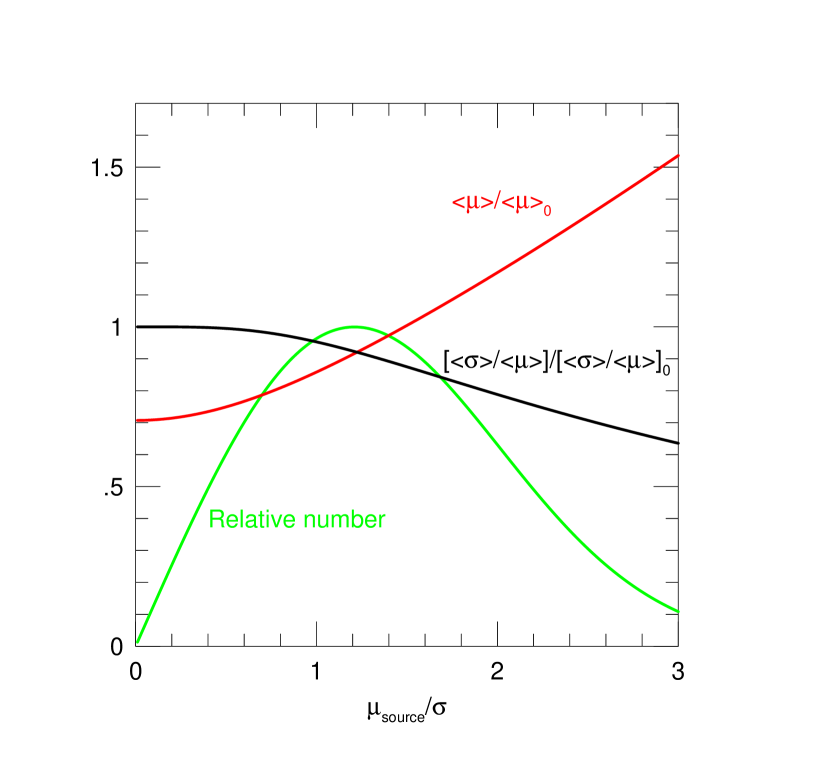
Figure 5: Effect of making a measurement of the source proper motion in units of the 1-D source proper-motion dispersion. The red curve shows the expected proper motion relative to the case of no measurement of ${\mbox{\boldmath$\mu$}}_{s}$, while the black curve shows a similar comparison for the fractional error in the $\mu_{\rm rel}$ estimate. Given Equation (13), these comparisons are exactly the same for the mass estimate. Hence, for example, if $\mu_{s}=0$, then the mass estimate should be reduced by $\sqrt{2}$ but the fractional error is exactly the same. On the other hand, if $\mu_{s}=2\sigma$, then the mean mass estimate is 17% higher than the no-$\mu_{s}$-measurement case, while the fractional error drops to 79% of the no-$\mu_{s}$-measurement case. The green curve shows the relative number of events with $\mu_{s}$ at various values. This plot is constructed assuming that the directional information from the parallax measurement is ignored.

where we have adopted $\langle\theta_{*}\rangle=0.5\,\mu{\rm as}$ as the mean radius of G dwarfs, defined as $3.5<M_{I}<5$. We estimate $N_{\rm G}$, the surface density of G dwarfs, by doubling the number within $3.5<M_{I}<5$ in Figure 5 of Holtzman et al. (1998). We extrapolate this diagram to estimate the surface density of stars as $5\times 10^{4}/{\rm arcmin^{2}}$, then double this number to consider a better microlensing field, and then multiply by five based on the 5:1 FFP/star ratio estimated by Mróz et al. (2017). We approximate the bulge proper-motion distribution as an isotropic Gaussian with dispersion $\sigma=2.9\,{\rm mas}\,{\rm yr}^{-1}$ based on experience with Gaia proper-motion data in many high event-rate fields. This functional form implies $\langle\mu\rangle=(4/\sqrt{\pi})\sigma$. See Appendix.

Next we repeat this calculation for three other brighter classes of stars, turnoff/subgiants ($2<M_{I}<3.5$), lower-giant-branch ($0.5<M_{I}<2$), and upper-giant-branch+red-clump ($M_{I}<0.5$). For the four classes, we adopt surface-density ratios (1.000, 0.267, 0.027, 0.025) and cross sections $2\langle\theta_{*}\rangle=(1.0,2.4,9.0,14.0)\mu{\rm as}$. The product of these factors is $(1.00,0.64,0.24,0.35)$. Hence, scaling to Equation (7), these yield respective rates

$${d\Gamma\over d\Omega}\Biggl{(}\matrix{\rm G\ dwarfs\cr\rm Turnoff/Subgiants\cr\rm Lower\ Giants\cr\rm Upper\ Giants}\Biggr{)}=\Biggl{(}\matrix{9.8\cr 6.2\cr 2.3\cr 3.4}\Biggr{)}{{\rm yr}^{-1}\over{\rm deg^{2}}}.$$ (8)

The first point to note regarding Equation (8) is that there can be a large number of potential FFP mass measurements, provided that some or all of these regimes can actually be probed. There are about $10\,{\rm deg}^{2}$ of high event-rate fields in the southern bulge that have modest extinction, $A_{I}\lesssim 2$, for which the G-dwarf limit would require $I_{\rm lim}\sim 21.5$. Now, it is certainly not possible to properly characterize magnification $A\sim 2$ events on $I=21.5$ sources from any current ground-based surveys, so the simplest implementation of this approach (coupling a new observatory orbiting at L2 with existing ground-based surveys) could not reach this limit.

However, the defining target of the first survey would be the bulge analogs of the $\theta_{\rm E}\sim 6\,\mu{\rm as}$ disk FFP population that has already been detected, i.e., with $\theta_{\rm E}=(16/125)^{1/2}6\,\mu{\rm as}=2\,\mu{\rm as}$. To be sensitive to a broad range of bulge $\pi_{\rm rel}$, we adopt a more conservative fiducial value of $\theta_{\rm E}=1.5\,\mu{\rm as}$. For these, $\rho=\theta_{*}/\theta_{\rm E}=0.33$ and so the peak magnification is $A_{\rm max}=\sqrt{1+4/\rho^{2}}\rightarrow 6$, implying a difference-star magnitude of $I=19.8$. Such an event probably could not be reliably recognized in ground data alone. However, if the L2 telescope had substantially better data, and in particular could determine $t_{\rm E}$ and $\rho$, then the fit to the ground-based light curve would be highly constrained (the reverse of the situation considered by Gould 1995; Boutreux & Gould 1996; Gaudi & Gould 1997). The situation would be substantially better for G dwarfs in the middle of the distribution, i.e., a factor 2 brighter.

We now turn to the opposite extreme: giant sources. The same bulge super-Earth discussed above would magnify only a small part of a clump giant’s $(\theta_{*}=6\,\mu{\rm as})$ surface, implying $A_{\rm max}=1.12$ and so $I_{\rm diff}=18.8$, i.e., a magnitude brighter than the G-dwarf case. The background (due to the giant itself) is higher, but this is overall a secondary effect.

The lower-giant branch stars have similar color, so similar surface brightness. Because only a portion of their surface would be magnified by a $\theta_{*}=1.5\,\mu{\rm as}$ lens, the difference star would have similar brightness $I_{\rm diff}=18.8$. Moreover, the source itself would generate less background noise.

The best case would be the turnoff/subgiants because they have higher surface brightness. For example, for $M_{I}=3$ and $\theta_{*}=1.2\mu{\rm as}$, $I_{\rm diff}=18.6$. That is, all four classes in Equation (8) could potentially contribute to FFP detections, although it will still be necessary to examine the integrated measurement process as a whole.

In brief, there is a known population of 12 FFPs, of which 11 are likely due to super-Earths, mostly in the disk (Ryu et al., 2020), with five of these 11 having measured $\theta_{\rm E}\sim 6\,\mu{\rm as}$. If there are analogs of these objects in the bulge (with $\theta_{\rm E}\sim 1.5\,\mu{\rm as}$), then none have been detected in current surveys, and the sensitivity of these surveys to such objects is limited. However, even at the adopted $M_{I}\sim 5$ threshold, ground surveys could marginally characterize the light curve generated by such putative bulge super-Earths, provided that $(\rho,t_{\rm E})$ were well determined from space. This would permit a marginal mass measurement at this threshold. Mid-G dwarf and brighter sources would yield substantially better results.

4 KMTNet + L2 Satellite (KMT+L2)

In this and the next section, we will consider two of the many possible two-observatory scenarios that could probe the FFP mass and distance functions. We begin this section by motivating why combining the KMTNet survey (Kim et al., 2016) with an L2 satellite (KMT+L2) should be one of those subjected to review.

First, KMT+L2 is an intrinsically cheap option. The satellite requirements are limited by the fact that whatever FSPL events that it might detect that are “inaccessible” to KMTNet (in the sense that they cannot be characterized with ground-based data even if $t_{\rm E}$ and $\rho$ are known infinitely well from space) are useless.

Second, such a low-requirement satellite could be built very quickly, while KMTNet is still in operation (or could be persuaded to remain in operation). Thus, it could return results on FFPs before it is absolutely confirmed that the bulk of the FFP candidates that have been reported to date are FFPs (rather than wide-orbit planets).

Note that while wide-orbit planets, if they exist, would be just as interesting and important as FFPs, they do not require such specialized equipment to measure their mass and distance functions. The very same 30m AO followup that would prove that the FFP candidates have hosts, would also measure the mass and distance of these hosts, while second AO epochs would yield the host-planet separations (Gould, 2016; Ryu et al., 2020).

Therefore, the low cost of KMT+L2 is well matched to the higher risk that the target population may be non-existent.

Third, by obtaining early results, KMT+L2 could influence the design of more advanced experiments that would be motivated by AO confirmation of earlier FFP candidates. For example, Ryu et al. (2020) show that FFP candidates (OGLE-2016-BLG-1540, OGLE-2016-BLG-1928, OGLE-2012-BLG-1323, KMT-2017-BLG-2820) (Mróz et al., 2018, 2020, 2019; Ryu et al., 2020) can be confirmed (or ruled out) as FFPs by (2024, 2024, 2027, 2028), respectively.

Fourth, as we will show, any experiment designed to measure masses and distances of FFPs will automatically return these same measurements for a large fraction of bound-planet lenses in its field of view. Such measurements will remain of exceptional interest only until the advent of 30m AO, at which point such mass and distance measurements will generally be possible after wait times of 3–5 years. The exception is that two-observatory experiments will also yield masses and distances for dark (e.g., brown dwarf, white dwarf) hosts, whereas AO followup will not.

As a specific example, we will consider a 0.3m optical telescope in L2, equipped by a 18k$\times$18k camera. This choice is partly motivated by the actual design of a planned multi-telescope satellite (Earth 2.0 Transit Survey Mission), which will mainly be utilized for transits, but which could include a microlensing telescope, and partly because a 0.3m telescope would yield photometry that is significantly (but not dramatically) better than KMTNet at the faint end, in accordance with the first motivating point given above.

We will assume a throughput similar to KMTNet and a filter similar to $I$-band as well. These imply a FWHM = $0.67^{\prime\prime}$ and photometric zero point of $I_{\rm zero}=26.75$ for a nine-minute exposure, i.e., 200 photons from an $I=21$ difference star.

We now consider a specific implementation with a $2^{\circ}\times 2^{\circ}$ field of view and $0.40^{\prime\prime}$ pixels, i.e., identical to KMTNet. The camera would be centered and oriented to exactly match the KMT observations. The center would be at about $(l,b)=(+1.0,-1.8)$ if the KMTNet cameras can be rotated to Galactic coordinates and about $(l,b)=(+1.0,-2.1)$ if they cannot. The blue dots in Figure 8 of Ryu et al. (2019) show published planetary microlensing events from 2003–2010, a period when microlensing survey cadences were adequate to find events over a broad area, but mostly could not characterize planetary perturbations by themselves. Rather, planets were mostly found by targeted follow-up observations of these events (Gould & Loeb, 1992). The distribution is quite broad over the southern bulge, although it does favor regions that are closer to the plane. Hence, the huge concentration of planet discoveries centered on $(l,b)=(+1.0,-1.8)$ from subsequent years is mainly a product of the fact that much higher-cadence surveys concentrated on these areas. Nevertheless, KMTNet’s choice to concentrate on this area with its highest cadence fields (red field numbers) does reflect the highest intrinsic event rate as determined using the method of Poleski (2014).

At $(0.67/0.40)=1.7\,$pixels/FWHM, the images would be slightly subsampled, but still much better sampled than for $3.6\mu$m observations on Spitzer: 0.9 pixels/FWHM. And the photometry would benefit from the much more uniform pixel response function characteristic of optical CCDs. Hence, it is plausible that photon-limited photometry could be achieved. Considering the point spread function (PSF) of $\pi\,{\rm FWHM}^{2}=1.4\,{\rm arcsec}^{2}$, there would be about 1.5 G dwarfs (similar to the target source population) per PSF. Hence, an $A=2$ magnification event (of an $M_{I}=4.5$, $A_{I}=2$ star) would have a 200 photon signal and $\sqrt{200\times 2.5}\sim 25$ photon noise (assuming good read noise, etc), i.e., a signal-to-noise ratio (SNR) of 8. With 10 such exposures over a typical $2\,t_{*}=1.6\,$hr event, there would be a clear detection and reasonable characterization of extreme $\theta_{\rm E}=\theta_{*}\sim 0.5\,\mu{\rm as}$ FFPs. However, because this same event could barely be “detected” from the ground (even if one knew from the space observations where to look), there would be no parallax measurement. Still, the “routine” detection of such small-$\theta_{\rm E}$ FSPL events would be of considerable interest. By contrast, only one such $\theta_{\rm E}<1\,\mu{\rm as}$ event has been detected in 10 years of OGLE-IV data (Mróz et al., 2020).

Because $\theta_{*}=0.5\,\mu{\rm as}$ is already in the $\rho\gtrsim 1$ limit for which the excess flux is basically just twice the area of the Einstein ring times the surface brightness, the brighter three classes have similar excess fluxes.

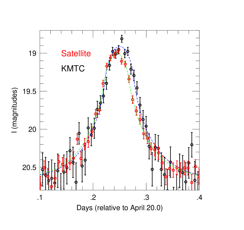
Figure 2: Concrete realization of observations of the event shown in Figure 1 with simulated Gaussian noise. The noise is applied to the flux, with the values and errors transformed to magnitudes for plotting. Note that, even in the presence of scatter, the differences in center, width, and height between the two curves is discernible by eye.

On the other hand, as discussed in Section 3, for putative bulge super-Earth FFPs of $\theta_{\rm E}=3\,\theta_{*}\sim 1.5\,\mu{\rm as}$, the satellite would yield excellent characterization and, based on the resulting $(\rho,t_{\rm E})$ measurements, the ground light curve could be well characterized. See Figures 1 and 2.

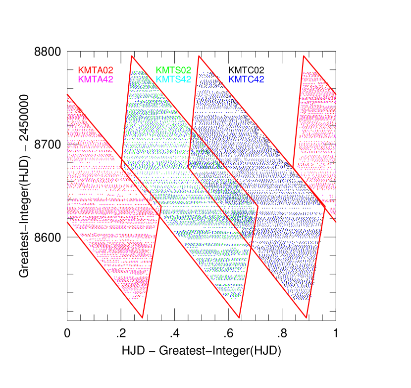
Figure 3: Day versus time of actual 2019 observations of closely overlapping KMT fields BLG02 and BLG42, color coded as indicated in the legend for the three KMT observatories: KMTA, KMTS, and KMTC. The red quadrangle around the KMTC observations is the empirically determined limit of the observational window for that field. Note that KMT does not observe in the extreme wings of the season, but could in principle. The remaining two red quadrangles are translated versions of the KMTC quadrangle. They match the empirical boundary of KMTS very well, but the match is less perfect for KMTA. Nevertheless, it is satisfactory for present purposes. See Figure 4.

However, the true rate of measurements would be well below that implied by Equation (8) simply because these require simultaneous observations. While the L2 observations could be carried out continuously (apart from a short window when the Sun passes through the bulge), the combined three KMTNet telescopes can observe a given bulge field 49% (after taking account of a 3% overlap between KMTS and KMTC) of the year due to the annual and diurnal cycles. See Figure 3. For about 1/4 of this 49% (averaged over the 3 telescopes), bad weather or high background would prevent useful observations, leaving about 37%. For about 30% of this remaining time, the projected separation would be $D_{\perp}<0.5D$ due to the alignment of Earth, L2, and the bulge near (June 20)$\pm$(1 month). This would degrade parallax measurements for small $\pi_{\rm rel}$, in some cases critically. We estimate that KMTNet and the L2 satellite would be able to work together about 28% of the year. Equation (8) then implies that a 4 year mission would make mass/distance measurements for about 100 bulge super-Earth FFPs. There are, intrinsically, about 5 times fewer corresponding disk FFPs. However, due to their roughly 8 times larger $\pi_{\rm rel}$ (and corresponding $\sim 2.8$ times larger $\theta_{\rm E}$), they are hardly affected by the contraction of $D_{\perp}$ near opposition. Moreover, the peak magnification for FSPL events is more than 1 magnitude greater, meaning that 1 additional magnitude from the Holtzman luminosity function is accessible. Hence, we estimate roughly 30 measurements of disk FFPs from the same population. In addition, it is plausible that the FFP mass function rises toward lower (e.g., Earth and Mars) masses, in which case the experiment would be sensitive to those as well, but only in the disk.

Table 1 summarizes the adopted properties of the KMT+L2 system, and Table 2 summarizes the prospective FFP detections as a function of source type and lens population.

4.1 Source Color Measurements

The determination of $\theta_{\rm E}$ requires that the source color be measured, or at least accurately estimated. The best way to do this is to take data in two bands during the event, and either fit them both to a common model, or just perform linear regression on the fluxes. In the present case, the only source of data in a second band will be KMT $V$-band data. For the marginal events just described, with difference magnitudes $I_{\rm diff}=21$, the $V$-band difference magnitudes will be $V_{\rm diff}=I_{\rm diff}+(V-I)_{0}+E(V-I)\rightarrow I_{\rm diff}+2.2$ for $(V-I)_{0}=0.7$ and $E(V-I)=1.5$. This will not be measurable in the most extreme cases $I_{\rm diff}=21$, for which it will be necessary to estimate the color, either from that of the baseline object (see Section 4.2) or from the fitted source flux (or even baseline flux) together with a color-magnitude diagram. The former method can work quite well provided that the baseline images are resolved to the depth of the source flux. The latter can lead to errors in $\theta_{\rm E}$ (and so $M$) of $\sim 15\%$ for main-sequence stars and turnoff stars.

However, for the defining targets, bulge super-Earths with $\theta_{\rm E}\sim 1.5\,\mu{\rm as}$, a turnoff source, $M_{V}=3.7$, $\theta_{*}=1.2\,\mu{\rm as}$ and $A_{V}=3.5$, together imply $V_{\rm diff}=21.2$. This corresponds to about 1000 difference photons in a 75 second exposure, of which there would be a dozen over peak. Hence, there would be many robust color measurements as well as some estimated colors with larger error bars.

4.2 CSST Imaging for Baseline-Object Color and Blending

The Chinese Space Station Telescope (CSST) is a 2m wide-field ($1.2\,{\rm deg}^{2}$) imager with 75 mas pixels, scheduled for launch in 2024. There is no filter wheel, but sections of the focal plane are allocated to various pass bands, including SDSS $(g,r,i,z,y)$, with FWHM=(60,82,98,123,136) mas. Hence, the entire KMT+L2 $4\,{\rm deg}^{2}$ field could be covered in $griy$ in 200 overlapping pointings, with about 90% of the area imaged twice in each band.

At this resolution, and at the depth relevant to the experiment, the field is essentially “empty”, i.e., just $6\,\times 10^{-3}$ G dwarfs per pixel. In most cases, the event could be localized to 0.1 KMT/L2 pixels (40 mas) from difference imaging. Hence, very few ambient stars would be mistaken for and/or blended with the source. That is, the potential blends would be essentially restricted to companions of the source or lens. For cases that the source flux derived from the fit was in tight agreement with that of the corresponding baseline object, the baseline-object color would be an excellent proxy for the source color. In other cases, one could adopt the color and magnitude of the baseline object, together with a suitable statistical distribution based on properties of potential lens and source companions. This entire procedure could be rigorously tested on hundreds of high-magnification microlensing events, for which the $(V-I)$ color will be precisely measured by KMT.

4.3 Discrete and Continuous Parallax Degeneracies

Refsdal (1966) already pointed out that satellite parallax determinations are subject to a four-fold degeneracy because we infer ${\mbox{\boldmath$\pi$}}_{\rm E}=\Delta{\bf u}({\rm au}/D_{\perp})$ from a measurement of the offset in the Einstein ring, $\Delta{\bf u}=(\Delta t_{0}/t_{\rm E},\Delta u_{0})$, from the fit parameters $(t_{0},u_{0})$ to the ground and satellite light curves. However, while $u_{0}$ is a signed quantity, only its modulus can generally be determined from the light curve of short events. Thus, there are two solutions with the source passing on the same side of the lens as seen by both observatories, $(+,+)$ and $(-,-)$, and two with the source passing on opposite sides, $(+,-)$ and $(-,+)$. The two members of each pair have the same $\pi_{\rm E}$ but different directions. However, the first pair has smaller $\pi_{\rm E}$ than the second: $\pi_{{\rm E},\pm,\pm}<\pi_{{\rm E},\pm,\mp}$. See Figure 1 from Gould (1994b). For the very short events under consideration here, the only way to rigorously break this degeneracy is to observe the event from a third observatory (Refsdal, 1966) as was done in the cases of (OGLE-2007-BLG-224, OGLE-2008-BLG-279, MOA-2016-BLG-290) (Gould et al., 2009; Yee et al., 2009; Zhu et al., 2017).

The only other path to distinguishing between $\pi_{{\rm E},\pm,\pm}$ and $\pi_{{\rm E},\pm,\mp}$ is statistical: if $\pi_{{\rm E},\pm,\pm}\ll\pi_{{\rm E},\pm,\mp}$ (i.e., $\Delta u_{0}\ll u_{0}$) then the latter solution requires fine tuning (J. Rich, circa 1997, private communication; Calchi Novati et al. 2015). In fact, the “Rich Argument” factor appears naturally as a Jacobian within a standard Bayesian analysis (Gould, 2020).

For KMT+L2 FFP parallax measurements, the “Rich argument” will often prove applicable to giant-source events. For example, according to Equation (3), for a lower-giant-branch source ($\theta_{*}=3\,\mu{\rm as}$) and a bulge lens $\pi_{\rm rel}=16\,\mu{\rm as}$, the offset between the two observatories will be 0.054 source radii. Hence, for $u_{0}\sim\rho/2$, $\pi_{{\rm E},\pm\mp}/\pi_{{\rm E},\pm\pm}\sim 20$. That is, the lens will transit the source at similar (source) impact parameters, and it would require fine tuning to arrange that they transited at almost symmetric impact parameters. In addition, for cases that $\rho\ll 1$, so that $u_{0}\ll\rho$ is necessarily small as seen from one observatory (to have an FSPL event), then the lens trajectory may fall well outside the source as seen from the other observatory, in which case $\pi_{{\rm E},\pm,\pm}\simeq\pi_{{\rm E},\pm,\mp}$, so there is no real degeneracy. However, particularly for $\rho\sim 1$, which includes the most extreme and difficult lenses, there may be significant ambiguity in the interpretation of individual events.

This discrete degeneracy interacts with the continuous degeneracy in $\Delta u_{0}$. If the source flux is left as a free parameter for a 1L1S (more specifically FSPL) event, then the error in $u_{0}$ will in general be much larger than the error in $t_{0}/t_{\rm E}$. Therefore, if the two $u_{0}$ from the two observatories are treated as independent parameters, then the error in $\Delta u_{0}$ will be correspondingly greater than in $\Delta t_{0}/t_{\rm E}$. However, if the ratio of source-flux parameters $f_{s}$ is constrained from comparison stars, then the error in $\Delta u_{0}$ can be greatly reduced, but only for the small $\pi_{\rm E}$ solution. See Equation (2.5) of Gould (1995) for the first example of a calculation of this effect. The reason is that as the flux is varied, the two values of $|u_{0}|$ move in tandem. For the small-parallax solution, this means that the two values of $u_{0}$ also move together, but for the large-parallax solution, they move oppositely.

For relatively bright sources, the issue of continuous degeneracies can be removed if a good argument can be made that the source is unblended, so that the source flux can be fixed. In the general case, the same argument can ultimately be made after followup AO observations show the source and (possible) host in isolation. Then the source flux can be measured (and transformed to $I$ band), thereby greatly reducing the continuous degeneracy. If the source and host both appear, then the vector proper motion can be measured, which will very likely completely resolve the four-fold degeneracy (see Figure 1 of Gould 1994b). Of course, this will not include the cases of genuine FFPs. For some fraction of these, there will be $\sim{\cal O}(2)$ errors in the mass estimate due to unresolved four-fold degeneracies.

4.4 Bound Planets: Masses and Distances

KMT+L2 would have many other applications. We focus here on those that rest on combined mass and distance determinations for microlensing events, i.e., combined $\theta_{\rm E}$ and $\pi_{\rm E}$ measurements. First among these are binary-lens single-source (2L1S) events, particularly those containing planets.

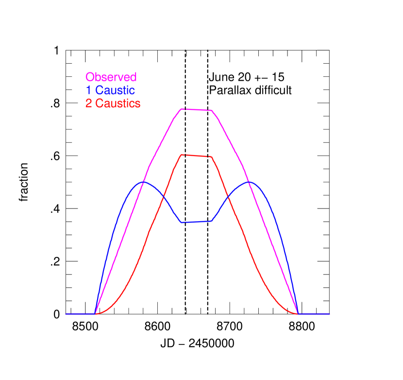
Figure 4: Fraction of time that A: a given 1L1S event can be observed by some KMT observatory (magenta); B: exactly one caustic of a given 2L1S event can be observed by some KMT observatory (blue); and C: both caustics of a given 2L1S event can be observed by some KMT observatory (red), assuming that KMT(A,S,C) are incapacitated by weather/Moon (35,25,15)% of the time. Hence, in the parts of the season that the red quadrangles in Figure 3 do not overlap, the magenta curve is simply 75% of the time that a given day lies inside one of these quadrangles. When they do overlap, account is taken of the fact that observations could take place at either observatory. Then, $f_{\rm red}=f_{\rm magenta}^{2}$ and $f_{\rm blue}=2(f_{\rm magenta}-f_{\rm red})$. The black dashed lines indicate the times of $D_{\perp}<0.0025\,{\rm au}$ (when 2L1S $\pi_{\rm E}$ measurements are very difficult) under the assumption that the satellite is exactly at L2. In fact, L2 orbits have a minimum $24^{\circ}$ in-plane motion, so this “dead zone” will actually lie somewhere $\pm 25\,$days from where it is shown. However, this is a minor effect. For 1L1S, the range of “difficult” parallax measurements (not shown) is about two times longer.

Graff & Gould (2002) pointed out that 2L1S events were ripe for mass measurements by a parallax satellite because (in contrast to the overwhelming majority of 1L1S events) ground-based data routinely return measurements of $\theta_{\rm E}$ due to finite-source effects during caustic crossings. This in turn is due to the facts that the caustics are much larger for 2L1S and (very importantly) that we mainly become aware of the lens binarity due to such caustic crossings. Hence, all that is needed to complete the mass and distance determinations is a $\pi_{\rm E}$ measurement. Graff & Gould (2002) investigated a number of problems related to such measurements (including the role of degenerate solutions – see their Figure 4), but they did so within the context of an Earth-trailing parallax satellite that would be triggered to sparse observations by a ground-based alert.

Gould et al. (2003) studied a problem much closer to the present one: a survey telescope at L2, complemented by a simultaneous ground-based survey. However, their main concern was to investigate the possibility of measuring $\pi_{\rm E}$ and $\theta_{\rm E}$ for Earth-mass planets even in the absence of a caustic crossing (see their Figure 1). They comment in passing that such a ground+L2 survey will routinely yield $\pi_{\rm E}$ plus $\theta_{\rm E}$ measurements for caustic crossing events, but they do not further explain this.

Here, we discuss to what extent this is actually the case. We begin by asking what can be learned from observations of the source crossing a single caustic, combined with a model of the caustic geometry derived from the overall light curve as observed from a single observatory (say, the satellite). In particular, the crossing will take place at an angle $\phi$ (where $\phi=0$ corresponds to perpendicular). Then, as seen from Earth, the crossing will take place $\Delta t=\Delta t_{0}+\tan\phi\Delta u_{0}t_{\rm E}$ later as seen from Earth, where $(\Delta t_{0}/t_{\rm E},\Delta u_{0})\tilde{r}_{\rm E}$ is the offset between the two observatories in the Einstein ring. If only $\Delta t$ is measured (no matter how precisely), one can gain only one constraint on the vector $\Delta{\bf u}=(\Delta\tau,\Delta\beta)\equiv(\Delta t_{0}/t_{\rm E},\Delta u_{0})$, and hence cannot uniquely determine $\pi_{\rm E}=\Delta u\,{\rm au}/D_{\perp}$. In principle, there is additional information from the difference between the “strength” of the caustic at the positions crossed by the source as seen from the two observatories. A “stronger” caustic will lead to a greater magnification at the peak of the crossing. However, except near the cusps, the gradient in caustic strength is very weak, meaning that in practice it is difficult or impossible to extract useful information from the different caustic-peak fluxes. As pointed out by Gould et al. (2003), it is also possible to get an independent constraint from the one-dimensional annual parallax (Gould et al., 1994) measured from the overall light curve. This will be feasible in some cases, but not others, in particular those with short $t_{\rm E}$ and/or faint sources. Here we focus on extraction of $\pi_{\rm E}$ from the caustic features of the light curve alone.

As caustics are closed curves, every entrance will be matched by an exit. If delays $\Delta t_{1}$ and $\Delta t_{2}$ occur at crossing angles $\phi_{1}$ and $\phi_{2}$, and each is measured with precision $\sigma$, then the measurements can be expressed as two equations with two unknowns $(\Delta\tau,\Delta\beta)$,

$$\Delta t_{i}=(1\cdot\Delta\tau+\tan\phi_{i}\cdot\Delta\beta)t_{\rm E}\pm\sigma;\qquad(i=1,2),$$ (9)

whose covariance matrix is

$$c_{i,j}\biggl{(}\matrix{\Delta\tau\cr\Delta\beta}\biggr{)}={\sigma^{2}\over(\tan\phi_{2}-\tan\phi_{1})t_{\rm E}^{2}}\biggl{(}\matrix{\tan\phi_{2}&-\tan\phi_{1}\cr-1&1}\biggl{)}.$$ (10)

Thus, for example, if the crossings are on consecutive caustic segments (i.e., separated by one cusp) then $|\phi_{2}-\phi_{1}|$ is likely to be a few tens of degrees, so that $|\tan\phi_{2}-\tan\phi_{1}|^{-1}$ will be only of order a few. However, if the caustic segments are separated by two cusps (or three cusps for some resonant caustics), then they could be roughly parallel, leading to $|\tan\phi_{2}-\tan\phi_{1}|^{-1}$ being of order ten or even a few tens.

However, in most cases, the measurement of two different caustic-crossing time offsets will yield good mass and distance determinations. The first point is that the offsets themselves are of order

$$\Delta t\sim{D_{\perp}\over\tilde{v}}={D_{\perp}\over{\rm au}}\,{\pi_{\rm rel}\over\mu_{\rm rel}}=13\,{\rm min}{D_{\perp}\over 0.01\,{\rm au}}\biggl{(}{\pi_{\rm rel}\over 16\,\mu{\rm as}}\biggr{)}\biggl{(}{\mu_{\rm rel}\over 6.5\,{\rm mas}\,{\rm yr}^{-1}}\biggr{)}^{-1},$$ (11)

while the full caustic crossing times will be $2\,|\sec\phi|t_{*}=97\,{\rm min}\,\sec\phi(\theta_{*}/0.6\,\mu{\rm as})/(\mu_{\rm rel}/6.5\,{\rm mas}\,{\rm yr}^{-1})$. Hence, there will be many observations per crossing. Here, $\tilde{v}\equiv\tilde{r}_{\rm E}/t_{\rm E}$ is the lens-source relative velocity projected on the observer plane. Moreover, caustic crossings generally yield magnification jumps $\Delta A\sim{\cal O}(10)$, which are easier to detect than the $\Delta A\sim$few, level events that define the requirements of the FFP experiment.

The main difficulty is that both observatories must observe both caustics. This would be automatic for the L2 satellite during the time (perhaps eight months per year) of its continuous observation. However, the ground observations would face interruptions due to weather and diurnal cycle. Approximating the two caustic crossings as independent, and scaling weather/Moon interruptions as (15,25,35)% at KMT(C,S,A), then 22% of all events during the (365 day) year would be observed during two caustic crossing and another 29% would be observed during one. See Figure 4. As noted above, $\pi_{\rm E}$ could be recovered for some of the latter by combining the single caustic time offset with the 1-D annual parallax signal. Moreover, high-magnification events, which are especially prone to planetary anomalies (Griest & Safizadeh, 1998), will often yield parallax measurements even if planetary caustic crossings are not observed (Yee, 2013). We also note that if we exclude the 31 days closest to opposition, when both parallax signals will be much smaller (due to small $D_{\perp}$ and low projected acceleration of the satellite and of Earth), then these percentages drop to 17% and 26%, respectively.

5 Two-Satellite Experiment: IRx2

By launching two identical survey telescopes into orbits separated by $D\sim{\cal O}(0.01\,{\rm au})$, one could pursue substantially different science relative to KMT+L2 (Section 4). For example, one satellite could be at L2 and the other in a low-Earth polar orbit or in geosynchronous orbit at relatively high inclination.

The main value of having two identical satellites is that the experiment would not be fundamentally constrained by the limits of ground-based observations. These constraints include both time coverage and resolution. But the most important ground constraint comes from the high sky background in the infrared (IR).

To address the various choices, we first focus on the main potential scientific objectives. As we have discussed above, the effective limit of KMT+L2 in Einstein radii is $\theta_{\rm E}\gtrsim 1.5\,\mu{\rm as}$, which roughly corresponds to FFP masses $M\sim 6\,M_{\oplus}$ in the bulge or $M\sim 0.7\,M_{\oplus}$ in the disk. Bodies of the latter mass scale are relatively common in the solar system (two examples). However, bodies that are 100 times less massive, i.e., $M\sim 0.5M_{\rm Moon}$ are more common, even though they are substantially more difficult to detect. In the context of the Solar System, such bodies could plausibly have been prodigiously “ejected” to the Oort Cloud or to unbound orbits, or they could remain “hidden” in the outer regions of the Kuiper Belt. Hence, the systematic study of such objects, both bound to and unbound from other stars, would give enormous insight into planetary-system formation and evolution. In particular, the FFP candidates with measured parallaxes and vector proper motions could be identified as part of the Oort Cloud of their hosts, even at several $10^{4}\,{\rm au}$, because the “background” of ambient field stars could be drastically reduced by demanding common proper motion and distance (Gould, 2016).

To reach the goal of $\theta_{\rm E}\sim 0.15\,\mu{\rm as}$ requires one to probe $\theta_{*}\sim 0.3\,\mu{\rm as}$ sources, which corresponds to $M_{\rm source}\sim 0.5\,M_{\odot}$. In this case, $\rho\sim 2$, so $A_{\rm max}\simeq\sqrt{1+4/\rho^{2}}\sim 1.4$. These $M_{I}\sim 6.5$ sources are a few times more common than G dwarfs, but also have only half the cross section $(2\,\theta_{*})$. Therefore, the underlying rates are similar. The main difficulty is that the difference-star magnitude at $A_{\rm max}=1.4$ and extinction $A_{I}=2$ is $I_{\rm diff}=24.1$. To obtain 10% photometry in a 9-minute diffraction-limited exposure would require a $D\sim 2$m diameter mirror.

An alternative would be a broad $H$-band filter similar to that of the Nancy Grace Roman (f.k.a WFIRST) telescope (Spergel et al., 2013). At $H_{\rm diff}=21.1$, a 9-minute exposure on a 0.5m telescope (with diffraction-limited FWHM$\sim 0.8^{\prime\prime}$), would yield 10% photometry. The same camera layout as KMT+L2 ($0.4^{\prime\prime}$ pixel scale, 18k$\times$18k detectors) would then imply Nyquist sampling. Thus, the telescope dimensions are qualitatively similar to KMT+L2, the main difference being that the former would be equipped with IR detectors. We dub this two-telescope system: IRx2.

Simultaneous observation by two identical telescopes plays a central role not only in measuring $\pi_{\rm E}$ (and so the FFP masses), but also in robustly distinguishing between extremely short, very faint microlensing events and various forms of astrophysical and instrumental noise.

The key problem is that for each square degree, and for a year of integrated observations. IRx2 would observe about $3\times 10^{7}$ early M dwarfs for 8760 hours, enabling $2.5\times 10^{11}$ independent probes for dwarf-planet FFPs/Exo-KBOs/Exo-OCOs. This might yield five detections or 5000 (per yr-deg²): there is no way to reliably estimate at this point. But how can one be sure that any one, or any 1000 of these are actually due to microlensing? One issue is instrumental noise. If the noise were Gaussian, then an $8\,\sigma$ signal would be enough to reject false positives at $p=\exp(-8^{2}/2)\sim 10^{-14}$. However, it would be difficult to rule out non-Gaussian noise in the detector or the detection system based on one observatory alone (such as Roman, which is expected to detect of hundreds of larger FFPs, Johnson et al. 2020). But this possibility would easily be ruled out if two observatories saw an event on the same star at nearly the same time.

A more fundamental problem is astrophysical noise. Suppose that one in a million early M dwarfs had one one-hour outburst per year. This would give rise to 30 “FFP events”. In fact, M dwarfs are known to have outbursts. In contrast to the case of instrumental noise, merely observing the same event from two independent telescopes would not guard against this astrophysical noise in any way: the effect is real, so all observers viewing it from the same place will see the same thing.

However, for IRx2, the event will look different as seen from the two observatories, i.e., delayed and/or with a different amplitude. The delay (tens of minutes) will be much longer than the light travel time between the observatories ($<5\,{\rm sec}(D/0.01\,{\rm au})$). There is no other effect that could cause delays, apart from interstellar refraction, which is not a strong effect at these wavelengths. Similar arguments apply to differences in the amplitude of the event as seen by the two observatories.

6 Parallax-only Events

Our focus in this paper has been on FFP mass measurements, $M=\theta_{\rm E}/\kappa\pi_{\rm E}$, derived from simultaneous measurements of $\theta_{\rm E}$ and $\pi_{\rm E}$. However, any experiment capable of delivering both parameters will yield many more measurements of $\pi_{\rm E}$ that are not complemented by measurements $\theta_{\rm E}$. In this section, we investigate the relative precision of mass estimates based on $\pi_{\rm E}$-only measurements, compared to measurements based on $\pi_{\rm E}$+$\theta_{\rm E}$. We then ask in what way and to what degree such estimates can augment our understanding of the FFP population and of other low-mass, non-luminous objects.

There are several previous studies that focused on L2-scale microlens parallax measurements. Zhu & Gould (2016) investigated combined KMTNet and Roman observations under the assumption that the latter would point at a relatively unextincted $(A_{H}\sim 0.5)$ field. In contrast to the KMT+L2 study that we carried out in Section 4, the Zhu & Gould (2016) L2 telescope was vastly more powerful than KMT, so that any event that was detectable by KMT had essentially perfect data from Roman. Nevertheless, we can use this study for some basic guidance to the issues discussed below.

Bachelet & Penny (2019) and Ban (2020) each studied joint observations by Euclid and Roman, both of which are planned to have L2 orbits. As mentioned above, “L2 orbits” have epicyclic radii of few$\times 10^{5}\,$km, around the mathematical “L2” point, so that the separation of these two satellites could be a large fraction of the Earth-L2 distance. They pursued complementary approaches. Bachelet & Penny (2019) applied a Fisher-matrix analysis to a narrow subset of possible events, while Ban (2020) subjected a detailed Galactic-model simulation to relatively simple cuts. In addition, Ban (2020) investigated joint LSST-Roman observations, as well as some other combinations.

All three studies note that finite-source effects impact an increasing fraction of events as the lens mass decreases. However, only Zhu & Gould (2016) make a quantitative estimate of this fraction. See their Figure 2.

6.1 Precision of Parallax-only Mass Estimates

Although satellite microlens-parallax measurements were proposed more than a half century ago (Refsdal, 1966) and have been a very active area of investigation for a quarter century (Gould, 1994b), it appears that no one has asked what is the fundamental limit of parallax-only microlens mass estimates. The key to doing so is a point already made by Han & Gould (1995): lens populations at different distances have very similar proper-motion distributions, $\mu_{\rm rel}=\theta_{\rm E}/t_{\rm E}$, but very different projected velocity distributions, $\tilde{v}=({\rm au}/\pi_{\rm rel})\mu_{\rm rel}$. Therefore, by measuring $\theta_{\rm E}$, or (because $t_{\rm E}$ is usually very well measured) equivalently $\mu_{\rm rel}$, one is only determining more precisely a quantity that is already “basically known”. By contrast, once $\pi_{\rm E}$ is measured, one can “guess” $\mu_{\rm rel}$ to reasonable precision and then estimate $M=\mu_{{\rm rel},\rm est}t_{\rm E}/\kappa\pi_{\rm E}$. Indeed this is how Ban (2020) estimated lens masses from the simulation results, which were then compared to the simulation input masses. Ban (2020) found, using $\mu_{{\rm rel},\rm est}=7.5\pm 1.5\,{\rm mas}\,{\rm yr}^{-1}$, that the scatter was larger than the assumed error, although the exact origin of this discrepancy could not be pinpointed because the simulation contained several other sources of error.

Let us initially consider a lens that is “known” to be in the bulge. For example, it could have $\tilde{v}=3000\,{\rm km}\,{\rm s}^{-1}$. Let us assume that $\pi_{\rm E}$ and $t_{\rm E}$ are measured very well. We can imagine trying to evaluate the lens mass by a Bayesian analysis using a Galactic model. If we ignore for the moment any prior on the lens mass, then the only relevant information from the model is the kinematic distributions of the sources and lenses, which are both drawn from the same approximately isotropic Gaussian, with dispersion $\sigma$. Then, this Bayesian analysis will return an analytic result (see Appendix),

$$M_{\rm est}={\mu_{{\rm rel},\rm est}t_{\rm E}\over\kappa\pi_{\rm E}}={t_{\rm E}\over\kappa\pi_{\rm E}}[\langle\mu_{\rm rel}\rangle\pm\sqrt{{\rm var}(\mu_{\rm rel})}]={\sigma t_{\rm E}\over\kappa\pi_{\rm E}}\biggl{[}{4\over\sqrt{\pi}}\pm\sqrt{6-{16\over\pi}}\biggr{]},$$ (12)

which then yields a fractional error in the mass estimate

$${\sqrt{{\rm var}(M)}\over M_{\rm est}}={\sqrt{{\rm var}(\mu_{\rm rel})}\over\mu_{{\rm rel},\rm est}}=\sqrt{{3\pi\over 8}-1}=0.42.$$ (13)

If we now add a mass prior, then it could somewhat change the mean estimate, but (unless it is very strong), it will not substantially change the standard deviation. Note that in the regime of FFPs, there is no basis for a strong prior (otherwise we would not be doing the experiment).

Because the $\mu_{\rm rel}$ distribution for disk lenses is very similar to that of bulge lenses, the fractional mass error is likewise similar. We have not as yet included the directional information that is returned by the ${\mbox{\boldmath$\pi$}}_{\rm E}$ measurement. However, for bulge lenses, this is completely irrelevant because the prior is essentially isotropic. And it is basically irrelevant if the lens is known to be in the disk because the directional distribution for ${\mbox{\boldmath$\mu$}}_{\rm rel}$ is basically independent of distance. For cases that the lens could be either in the disk or bulge, the directional information can help distinguish between these alternatives, but this cannot reduce the fractional mass-estimate error below the values derived under the assumption that the population is known.

Therefore, there is a hard limit of $42\%$ fractional mass-estimate error, even if the parallax is measured perfectly.

6.2 Improvement from Measuring ${\mbox{\boldmath$\mu$}}_{s}$

For the case of FFPs, there is no lens light, so the source proper motion ${\mbox{\boldmath$\mu$}}_{s}$ can be measured from two well separated high-resolution epochs. For example, we have suggested CSST observations.

Let us first imagine that such a measurement has been made, and it is found that ${\mbox{\boldmath$\mu$}}_{s}=0$ (in the bulge frame). Then, given this measurement, the estimated ${\mbox{\boldmath$\mu$}}_{\rm rel}$ distribution still has a mean of zero, but now its dispersion drops from $\sqrt{2}\sigma$ to $\sigma$. This means that the mass estimate drops by a factor $\sqrt{2}$ from what it would be without this measurement, but the fractional mass error, given by Equation (13) is still exactly the same. However, as $|{\mbox{\boldmath$\mu$}}_{s}|$ increases (in the bulge frame), there is increasing information constraining both the magnitude and direction. To illustrate this, we initially ignore the directional information and show the resulting mean mass estimate and fractional mass-estimate error (relative to the case of no source proper-motion measurement) in Figure 5.

The role of directional information is difficult to represent, in part because there are two directions that cannot be distinguished for short events without a third observatory at a similar distance from the first two (and even with such an observatory, breaking this directional degeneracy is difficult, Zhu et al. 2017). Therefore, we do not further pursue this analytic approach. The importance of the directional information can only be assessed by extensive Monte Carlo simulations. Nevertheless, as we have shown in Figure 5, ${\mbox{\boldmath$\mu$}}_{s}$ measurements can definitely contribute to the understanding of $\pi_{\rm E}$-only events.

6.3 Role of Parallax-Only Measurements

In the KMT+L2 experiment that we have described, for every bulge super-Earth with measurements of both $\theta_{\rm E}$ and $\pi_{\rm E}$, there will be of order one with a $\pi_{\rm E}$-only measurement. This can be understood by considering Figures 1 and 2: if the lens had passed outside the source (so dropping in amplified flux by a factor $\sim 2$) then the event would have already become much noisier. An additional factor of two would make parameter measurements difficult or impossible. Zhu & Gould (2016) reached similar conclusions for somewhat different assumptions. For the $t_{\rm E}\sim 0.3\,$day bulge events that we are considering, about half of all those with $\pi_{\rm E}$ measurements also had $\theta_{\rm E}$ measurements. See their Figure 2. Because the $\pi_{\rm E}$-only mass estimates have much larger errors, the addition of a comparable number of these to the $\pi_{\rm E}$+$\theta_{\rm E}$ sample will have marginal scientific impact.

However, the same is not true for higher-mass objects, such as free-floating Jupiters and low-mass brown dwarfs. First, these are almost certainly much rarer, and the number of FSPL events is directly proportional to the number density of the population. Hence, the number of direct mass measurements is likely to be tiny. Second, the ratio of $\pi_{\rm E}$-only to $\pi_{\rm E}$+$\theta_{\rm E}$ measurements is much greater. Consider for example, a lens that is 100 times more massive than the $\theta_{\rm E}\sim 1.5\,\mu{\rm as}$ example in Figures 1 and 2, i.e., right in the middle of the “Einstein desert” discussed by Ryu et al. (2020). With the same trajectory, it would be about 10 times brighter. Even passing at $\sim 5\theta_{*}$, it would be somewhat brighter than the event in those figures. Thus, $\pi_{\rm E}$-only measurements may be the only way to obtain mass estimates for this population.

7 Discussion

The basic physical principle, i.e., synoptic observations of FSPL events from two locations, is the same as that proposed by Gould (1997) for terrestrial-parallax mass measurements of “extreme microlensing” events. Gould & Yee (2013) later showed that the expected rate of such “extreme microlensing” mass measurements was only of order one per century under observing conditions of that time. Hence, they found it surprising that there were already two such measurements (Gould et al., 2009; Yee et al., 2009) when they published their analysis..

Because the physical principle and its mathematical representation are identical, it is worthwhile to understand the physical basis of the ${\cal O}(10^{3.5})$ difference in expected rates relative to the KMT+L2 experiment that we describe here.

Several factors are actually similar, including $\langle\mu\rangle=(10\,{\rm vs.}\,6.5){\rm mas}\,{\rm yr}^{-1}$, and $\langle\theta_{*}\rangle=(0.6\,{\rm vs.}\,0.5)\mu{\rm as}$, as well as the assumption that $(25\,{\rm vs.}\,28)\%$ of the year would be effectively monitored. Moreover, the total number of sources assumed by Gould & Yee (2013) was about 10 times higher because they considered potential follow-up observations of all Galactic bulge microlensing fields, whereas we have assumed continuous observations of just $4\,{\rm deg}^{2}$. However, this enhancement was canceled by the fact that only 1/10 of events would be observable at peak from multiple continents. Moreover, they estimated that only half of these would be successfully monitored (based on the statistical analysis of Gould et al. 2010).

The overwhelming majority of the difference comes from the fact that Gould & Yee (2013) estimated a surface density of lenses of $4.5\times 10^{2}\,{\rm arcmin}^{-2}$, whereas we have estimated $5\times 10^{5}\,{\rm arcmin}^{-2}$, i.e., a difference of $10^{3}$. A small part of this difference was in turn due to a different FFP model. In both cases, the lens surface density is dominated by FFPs, but Gould & Yee (2013) used the Sumi et al. (2011) model of two FFPs per star, whereas we have used the Mróz et al. (2017) model of five FFPs per star. However, the main difference was that Gould & Yee (2013) showed that the FSPL+terrestrial-parallax technique could only be applied to lenses within $D_{L}\lesssim 2.5\,{\rm kpc}$. That is, even with very good photometry on highly magnified events (such as OGLE-2007-BLG-224 and OGLE-2008-BLG-279) they considered that only events with $D_{\perp}/\tilde{R}_{*}>0.02$ would yield measurable parallaxes. Because $D_{\perp}\sim R_{\oplus}$ for terrestrial parallax (compared to $D_{\perp}\sim 250\,R_{\oplus}$ for L2 parallax), and because $\tilde{R}_{*}={\rm au}\theta_{*}/\pi_{\rm rel}$, the FSPL+terrestrial-parallax technique is restricted to lenses with high $\pi_{\rm rel}$.

8 Conclusions

The masses of FFPs can only be measured over a broad range of distances by simultaneous microlensing surveys conducted by two observatories separated by ${\cal O}(0.01\,{\rm au})$. Fortuitously, KMTNet can operate as one of these observatories. We show that a 0.3m telescope at L2, equipped with a KMT-like camera could be the other. Such a system would measure the masses of about 130 FFPs (from the known super-Earth population) over a 4-year mission, taking account of breaks in the observing schedule due to weather, Moon, and the diurnal and annual cycles. It could also discover lower-mass FFPs in the disk (down to Earth-mass or below), if these are equally common or more common. Finally, it would measure the masses and distances of many bound planets.

A next generation experiment, IRx2, consisting of two 0.5m IR satellites (at L2 and near Earth), could probe to sub-Moon masses, which are generally classified as “dwarf planets” rather than “planets”. These might actually be “free”, but could also be exo-KBOs and exo-OCOs. Once the mass, distance, and proper motion of these objects is found by IRx2, one epoch of AO followup can distinguish between these objects being “free” or part of exo-systems. If the latter, a second AO epoch can measure their projected separation from their host, and so determine whether they are exo-KBOs or exo-OCOs.

The duality and separation of the IRx2 system is crucial for verifying that the very weak and rare signals due to dwarf-planet FFPs are caused by microlensing rather than instrumental or astrophysical effects. The fact that there is signal from both satellites will prove that it is not due to instrumental effects. And the fact that the two signals are different (due to parallax) will prove that they are not due to astrophysical effects.

Appendix A $\langle\mu\rangle$ for Isotropic Gaussian

If ${\mbox{\boldmath$\mu$}}_{l}$ and ${\mbox{\boldmath$\mu$}}_{s}$ have isotropic 2-D Gaussian distributions with the same dispersions $\sigma$ and the same mean, then ${\mbox{\boldmath$\mu$}}_{\rm rel}={\mbox{\boldmath$\mu$}}_{l}-{\mbox{\boldmath$\mu$}}_{s}$ has a Gaussian distribution with zero mean and dispersion $s=\sqrt{2}\sigma$:

$$f(\mu_{x},\mu_{y})d\mu_{x}\,d\mu_{y}={\exp[-(\mu_{x}^{2}+\mu_{y}^{2})/2s^{2}]\over 2\pi s^{2}}d\mu_{x}\,d\mu_{y}={\exp[-\mu^{2}/2s^{2}]\over 2\pi s^{2}}d\mu_{x}\,d\mu_{y},$$ (A1)

where for simplicity, we have relabeled $\mu=\mu_{{\rm rel}}$. Then the mean value of $\mu$ weighted by the event rate (i.e., $\mu$ itself) is

$$\langle\mu\rangle={\int d\mu_{x}\,d\mu_{y}\,\mu\times\mu\,f(\mu_{x},\mu_{y})\over\int d\mu_{x}\,d\mu_{y}\,\mu\,f(\mu_{x},\mu_{y})}={\int_{0}^{\infty}2\pi\mu\,d\mu\mu^{2}\exp(-\mu^{2}/2s^{2})\over\int_{0}^{\infty}2\pi\mu\,d\mu\mu\exp(-\mu^{2}/2s^{2})}$$ (A2)

$$\langle\mu\rangle=2\,\sigma{\int_{0}^{\infty}dz\,z\exp(-z)\over\int_{0}^{\infty}dz\,z^{1/2}\exp(-z)}=2\,\sigma{1!\over(1/2)!}={4\over\sqrt{\pi}}\sigma,$$ (A3)

where $z\equiv\mu^{2}/4\sigma^{2}$. Similarly,

$$\sqrt{{\rm var}(\mu)}=\sqrt{\langle\mu^{2}\rangle-\langle\mu\rangle^{2}}=\sqrt{6-{16\over\pi}}\sigma.$$ (A4)

Table 1: KMT+L2 Telescope Properties

Property	KMT	L2
Aperture (m)	1.6	0.3
Cycle time (min)	8.25	10.0
$I$-band zero point	29.20	26.75
Pixel Size (arcsec)	0.40	0.40
FWHM (arcsec)	1.3–2.5	0.67
$I$-background (arcsec-2)	18.5	20.5
$I$-background (PSF-1)	16.7–15.3	20.1
$V$-band zero point	28.65
$V$-background (arcsec-2)	20.9

Note. — KMT “cycles” contain three 60s $I$- and one 75s $V$-band exposures. KMT background is sky dominated and is taken as 1.4 times “dark” value. L2 background is ambient-star dominated and is evaluated at $A_{I}=2$ and $2\times$Holtzman et al. (1998) luminosity function. Compare baseline and magnified performance of KMT vs. L2 in Figure1

Table 2: FFP Mass Measurements for KMT+L2

Characteristic	G dwarfs	MS/SG	Lower Giants	Upper Giants	Total
$\langle\theta_{*}\rangle\ (\mu{\rm as})$	0.5	1.2	4.5	7.0
$N_{\rm source}\ ({\rm arcmin}^{-2})$	3000	800	80	75
$2\langle\theta_{*}\rangle\langle\mu\rangle N_{\rm FFP,bulge}N_{\rm source}\Omega T_{{\rm eff},\rm bulge}$	44	28	10	15	97
$2\langle\theta_{*}\rangle\langle\mu\rangle N_{\rm FFP,disk}N_{\rm source}\Omega T_{{\rm eff},\rm disk}$	18	7	3	4	32

Note. — Assumes $\langle\mu\rangle=6.5\,{\rm mas}\,{\rm yr}^{-1}$, survey area $\Omega=4\,{\rm deg}^{2}$, $T_{{\rm eff},\rm bulge}=28\%(4\,{\rm yr})$, $T_{{\rm eff},\rm disk}=37\%(4\,{\rm yr})$, $N_{\rm FFP,bulge}=5\times 10^{5}\,{\rm arcmin}^{-2}$, $N_{\rm FFP,disk}=N_{\rm FFP,bulge}/5$, and that there are 1.4 times more accessible main-sequence (“G dwarf”) source for disk FFPs compared to bulge FFPs.

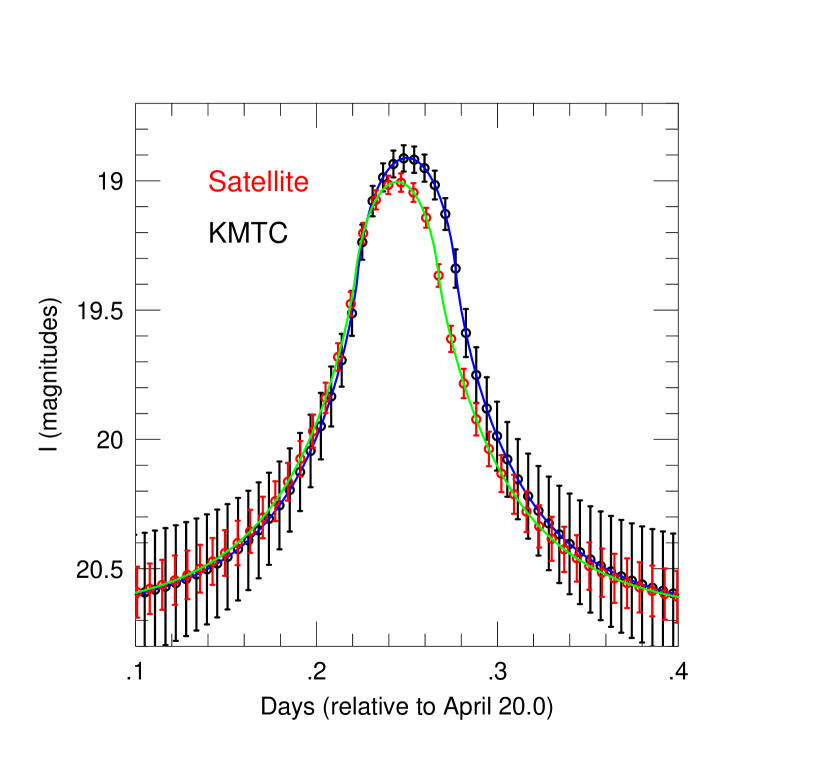
Figure 1: Illustration of light-curve data and error bars for KMTC (black) and a 0.3m satellite such as Earth 2.0 (red) for an $M=5.75\,M_{\oplus}$ lens lying in the Galactic bulge, $\pi_{\rm rel}=16\,\mu{\rm as}$ (e.g., $D_{S}=8.5\,{\rm kpc}$, $D_{L}=7.5\,{\rm kpc}$) magnifying a solar type source ($M_{I}=4$, $A_{I}=2$). These parameters yield $\theta_{*}=0.58\,\mu{\rm as}$. $t_{\rm E}=120\,$min, $t_{*}=46\,$min, $\rho=0.38$. For Earth $(t_{0},u_{0})=(0.2500\,{\rm day},0.2000)$, and for the satellite $\Delta(t_{0},u_{0})=(-7.9\,{\rm min},0.065)$. The displayed KMTC points are binned over 8.25 minute cycles, of three 1.00-minute $I$-band exposures, together with one 1.25 minute $V$-band exposure (not shown), with 1.00 minute read-out time. The satellite points have 9.0-minute integrations and 1.0-minute read out. In this case $\Delta t_{0}/t_{*}=17\%$. The four-fold degeneracy (Refsdal, 1966; Gould, 1994b) yields two solutions with the true parameters of the system, and another two with $(\Delta t_{0},|\Delta u_{0}|)=(-7.9\,{\rm min},0.465)$, which would imply $M=1.12\,M_{\oplus}$, $\pi_{\rm rel}=82\,\mu{\rm as}$, and $D_{L}=4.8\,{\rm kpc}$. This solution requires fine tuning and would be heavily discounted in a statistical analysis, but could not be ruled out in any individual case. See text. For a concrete realization with simulated noise, see Figure 2.

References

- Bachelet & Penny (2019) Bachelet, E., & Penny, M. 2019, ApJ, 880, L32
- Ban (2020) Ban, M. 2020, MNRAS, 494, 3235
- Bensby et al. (2013) Bensby, T. Yee, J.C., Feltzing, S. et al. 2013, A&A, 549A, 147
- Bessell & Brett (1988) Bessell, M.S., & Brett, J.M. 1988, PASP, 100, 1134
- Boutreux & Gould (1996) Boutreux, T. & Gould, A. 1996, 462, 705
- Calchi Novati et al. (2015) Calchi Novati, S., Gould, A., Udalski, A., et al., 2015, ApJ, 804, 20
- Delplancke et al. (2001) Delplancke, F., Górski, K.M., & Richichi, A. 2001, A&A, 375, 701
- Dong et al. (2019) Dong, S., Mérand, A., Delplancke-Strobale, F. 2019, ApJ, 871, 70
- Gaudi & Gould (1997) Gaudi, B.S. & Gould, A. 1997, ApJ, 477, 152
- Gould (1992) Gould, A. 1992, ApJ, 392, 442
- Gould (1994a) Gould, A. 1994a, ApJ, 421, L71
- Gould (1994b) Gould, A. 1994b, ApJ, 421, L75
- Gould (1995) Gould, A. 1995, ApJ, 441, L21
- Gould (1997) Gould, A. 1997, ApJ, 480, 188
- Gould (2016) Gould, A. 2016, JKAS, 49, 123
- Gould (2020) Gould, A. 2020, JKAS, 53, 99
- Gould & Loeb (1992) Gould, A. & Loeb, A. 1992, ApJ, 396, 104
- Gould & Yee (2013) Gould, A. & Yee, J.C. 2013, ApJ, 764, 107
- Gould et al. (2003) Gould, A., Gaudi, B.S., & Han, C. ApJ, 591, L53
- Gould et al. (1994) Gould, A., Miralda-Escudé, J. & Bahcall, J.N. 1994, ApJ, 423, L105
- Gould et al. (2009) Gould, A., Udalski, A., Monard, B. et al. 2013, ApJ, 698, L147
- Gould et al. (2010) Gould, A., Dong, S., Gaudi, B.S. et al. 2010, ApJ, 720, 1073
- Graff & Gould (2002) Graff, D.S. & Gould, A. 2002, ApJ, 580, 263
- Griest & Safizadeh (1998) Griest, K. & Safizadeh, N. 1998, ApJ, 500, 37
- Han & Gould (1995) Han, C. & Gould, A. 1995, ApJ, 447, 53
- Hog et al. (1995) Hog, E., Novikov, I.D., & Polanarev, A.G. 1995, A&A, 294, 287
- Holtzman et al. (1998) Holtzman, J.A., Watson, A.M., Baum, W.A., et al. 1998, AJ, 115, 1946
- Honma (1999) Honma, M. 1999, ApJ, 517, L35
- Johnson et al. (2020) Johnson, S.A., Penny, M., Gaudi, B.S., et al. 2020, AJ, 160, 123
- Kervella et al. (2004) Kervella, P., Thévenin, F., Di Folco, E., & Ségransan, D. 2004, A&A, 426, 297
- Kim et al. (2016) Kim, S.-L., Lee, C.-U., Park, B.-G., et al. 2016, JKAS, 49, 37
- Kim et al. (2018) Kim, D.-J., Kim, H.-W., Hwang, K.-H., et al., 2018, AJ, 155, 76
- Kim et al. (2020) Kim, H.-W., Hwang, K.-H., Gould, A., et al. 2020, AAS submitted, arXiv:2007.06870
- Mróz et al. (2017) Mróz, P., Udalski, A., Skowron, J., et al. 2017, Nature, 548, 183
- Mróz et al. (2018) Mróz, P., Ryu, Y.-H., Skowron, J., et al. 2018, AJ, 155, 121
- Mróz et al. (2019) Mróz, P., Udalski, A., Bennett, D.P.., et al. 2019, A&A, 622, A201
- Mróz et al. (2020) Mróz, P., , Poleski, R., Gould, A., et al. 2020, ApJ, 903, L11
- Miyamoto & Yoshii (1995) Miyamoto, M. & Yoshii, Y. 1995, AJ, 110, 1427
- Nataf et al. (2013) Nataf, D.M., Gould, A., Fouqué, P. et al. 2013, ApJ, 769, 88
- Nemiroff & Wickramasinghe (1994) Nemiroff, R.J., & Wickramasinghe, W.A.D.T. 1994, ApJ, 424, L21
- Poleski (2014) Poleski, R. 2016, MNRAS, 455, 3656
- Refsdal (1966) Refsdal, S. 1966, MNRAS, 134, 315
- Ryu et al. (2019) Ryu, Y.-H., Navarro, M.G., Gould, A. et al. 2019, AJ, 159, 58
- Ryu et al. (2020) Ryu, Y.-H., Mroz, P., Gould, A. et al. 2020, AAS submitted, arXiv:2010.07527
- Spergel et al. (2013) Spergel, D.N., Gehrels, N., Breckinridge, J., et al. 2013, arXiv:1305.5422
- Sumi et al. (2011) Sumi, T., Kamiya, K., Bennett, D. P., et al. 2011, Nature, 473, 349
- Witt & Mao (1994) Witt, H.J., & Mao, S. 1994, ApJ, 429, 66
- Walker (1995) Walker, M.A. 1995, ApJ, 453, 37
- Yee et al. (2009) Yee, J.C., Udalski, A., Sumi, T. et al. 2009, ApJ, 703, 2082
- Yee (2013) Yee, J.C. 2013, ApJ, 770, L31
- Yoo et al. (2004) Yoo, J., DePoy, D.L., Gal-Yam, A. et al. 2004, ApJ, 603, 139
- Zhu & Gould (2016) Zhu, W., & Gould, A., 2016, JKAS, 49, 93
- Zhu et al. (2017) Zhu, W., Udalski, A., Hwang, C.X., et al. 2017, ApJ, 849, L31