Distributed control under compromised measurements:
Resilient estimation, attack detection, and vehicle platooning

Abstract

We study how to design a secure observer-based distributed controller such that a group of vehicles can achieve accurate state estimates and formation control even if the measurements of a subset of vehicle sensors are compromised by a malicious attacker. We propose an architecture consisting of a resilient observer, an attack detector, and an observer-based distributed controller. The distributed detector is able to update three sets of vehicle sensors: the ones surely under attack, surely attack-free, and suspected to be under attack. The adaptive observer saturates the measurement innovation through a preset static or time-varying threshold, such that the potentially compromised measurements have limited influence on the estimation. Essential properties of the proposed architecture include: 1) The detector is fault-free, and the attacked and attack-free vehicle sensors can be identified in finite time; 2) The observer guarantees both real-time error bounds and asymptotic error bounds, with tighter bounds when more attacked or attack-free vehicle sensors are identified by the detector; 3) The distributed controller ensures closed-loop stability. The effectiveness of the proposed methods is evaluated through simulations by an application to vehicle platooning.

AND OR NOT TO COMMENT BODY IF ELSE ELSIF FOR WHILE

, ,

1 Introduction

Motivations and related work

Networked control systems (NCS) are ubiquitous. The performance of NCS significantly depends on widely deployed sensors which might be compromised due to the presence of malicious attackers [1, 2]. The attackers can strategically manipulate the sensor measurements in order to affect stability and performance of NCS. Attack detection, state estimation, and system control are three major components in the design of secure NCS in malicious environments.

To detect whether systems are under attack and identify attacked components, quite a few detection methods are proposed. Attack detection and identification for linear descriptor systems are studied in [3]. Methods of attack detection and correction for noise-free linear systems are proposed in [4]. To detect the Byzantine adversaries with quantized false alarm rates, [2] study a trust-aware consensus algorithm. In [5, 6], distributed detectors are designed for false data injection (FDI) attacks in communications. Detection and mitigation methods are proposed by [7] for distributed observers under a class of bias injection attacks. A joint detection and estimation problem is investigated in [8] with the knowledge of some attack statistics. There are some methods for multi-observer based detector design [9, 10, 11]. However, the computational complexity of these methods substantially increases as the number of sensors is increasing. Thus, designing single-observer based detectors without relying on the knowledge of attack signals needs more investigations. Moreover, most existing methods focus on detecting the attacked sensors, but few results are given for the identification of attack-free sensors.

There are two major approaches in the literature for handling state estimation under sensor attacks. The first approach is based on solving optimization problems [1, 12, 13, 14, 15, 16, 17]. This approach needs a large number of computational resources in enumerating all sensor combinations in order to find the attacked sensor set. Thus, it is not suitable to large-scale sensor networks if the resources are constrained. The second approach is to use robust techniques in handling potentially compromised data, such as discarding a few largest and smallest elements [18, 19, 20, 21], using the signum information of measurement innovations [22], and saturating the innovation which reaches a threshold [23, 24]. This approach is more suitable in online estimation since it needs very less computational resources than the first approach. However, there are few results in this direction, especially for dynamical systems under FDI sensor attacks.

Some resilient distributed control strategies have been proposed to achieve formation control of a group of vehicles or robots in malicious environments. There are strategies on how to handle different attacks, such as replay attack on control commands [25], denial-of-service (DoS) attack on measurement and control channels [26], FDI attack in the transmission from controller to actuator [27], attack on network topology of multi-agent systems [28], and stealthy integrity attacks [29]. However, there is no unified architecture integrating resilient estimation, attack detection and distributed control.

Contributions

In this paper, we propose an architecture comprising of a resilient observer, an online attack detector, and a distributed controller, such that a group of vehicles can achieve accurate state estimates and formation control even if the measurements of a subset of the vehicle sensors are compromised by a malicious attacker. The main contributions of this paper are summarized as follows:

1. We propose an adaptive resilient observer, designed by saturating the measurement innovation through a preset static or time-varying threshold, such that the potentially compromised measurements have limited influence to the estimation (Algorithm 1). Some essential properties are found: i) The observer is able to provide an upper bound of the estimation error at each time (Proposition 1); ii) If the observer threshold is static and satisfied with some explicit design principle (Proposition 2), the estimation error is asymptotically upper bounded (Theorem 1); and iii) If the observer threshold is time-varying and computed adaptively, the estimation error is also asymptotically upper bounded (Theorem 2) and the bound is tighter than that of the static threshold.

2. We develop an online distributed attack detector with the potentially compromised sensor measurements and the observer’s estimates. The designed detector is able to update three sets of vehicle sensors: the ones surely under attack, surely attack-free, and suspected to be under attack (Algorithm 2). Some properties are found: i) The detector is fault-free (Lemma 1), which differs from the existing results with false alarms (e.g., [2]); and ii) If some condition holds, all attacked and attack-free vehicle sensors are identified in finite time (Theorem 3);

3. We design a distributed controller (Algorithm 3) to achieve the formation control of the vehicles. We find that if the controller parameters satisfy some graph-related conditions, the overall performance function is asymptotically upper bounded in the presence of noise and tending to zero in the absence of noise (Theorem 4 and Corollary 1), which ensures the closed-loop stability of the proposed architecture.

The proposed observer is able to handle more typical sensor attacks than [8, 7], such as random attack, DoS attack, bias injection attack, and replay attack. The proposed detector is based on one observer, which requires less computational resources than the detectors based on multiple observers [9, 10, 11]. Although [20] study a wider range of attacks than this paper, we remove the requirements of graph robustness. Moreover, the sufficiently large communication times between two updates [30] is not required. Note that in comparison with our recent work [24], the current paper studies a different problem, and uses potentially compromised measurements with new approaches.

Outline

The remainder of the paper is organized as follows: Section 2 is on the problem formulation, followed by an overview of the proposed distributed observer-based control architecture in Section 3. Section 4 designs a resilient observer for each vehicle, based on which Section 5 studies the attack detection problem. In Section 6, a distributed controller is proposed to close the loop. After simulations of vehicle platooning in Section 7, the paper is concluded in Section 8. The main proofs are given in Appendix.

Notations: $\mathbb{R}^{n\times m}$ denotes the set of real-valued matrices with $n$ rows and $m$ columns, and $\mathbb{R}^{n}$ the set of $n$-dimensional real-valued vectors. Without specific explanation, the scalars and matrices in this paper are real-valued. Denote $\mathbb{N}^{+}$ the set of positive integers and $\mathbb{N}=\mathbb{N}^{+}\cup 0.$ The matrix $I_{n}$ stands for the $n$-dimensional square identity matrix. The superscript “$\sf T$” represents the transpose. The operator $\operatorname{diag}\{\cdot\}$ represents the diagonalization. We denote the Kronecker product of $A$ and $B$ by $A\otimes B$. The vector norm $\left\lVert x\right\rVert$ is the 2-norm of a vector $x$. The matrix norm $\left\lVert A\right\rVert$ is the induced 2-norm, i.e., $\left\lVert A\right\rVert=\sup_{x\neq 0}\left\lVert Ax\right\rVert/\left\lVert x\right\rVert$. The notations $\lambda_{\min}(A)$ and $\lambda_{\max}(A)$ are the minimal and maximal eigenvalues of a real-valued symmetric matrix $A$, respectively. The notation $a=(a_{i})_{i=1,2,\dots,n}$ is a vector consisting of elements $a_{1},\dots,a_{n}$. Let $\mathbb{I}_{i\in\mathcal{C}}$ be an indicator function, which equals 1 if $i\in\mathcal{C}$; otherwise, it is 0. The function $\lceil\cdot\rceil$ stands for the ceiling function.

2 Problem Formulation

In this section, we first motivate the problem through a vehicle platooning example, and then formulate the problem.

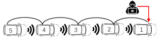
Figure 1: Platoon of five vehicles. The position and velocity measurements of vehicle 1 are compromised by a malicious attacker. Each vehicle is able to exchange messages with other vehicles nearby through wireless communication.

2.1 Motivating example

Consider the five-vehicle platooning in Fig. 1. The aim is to control the speed of all vehicles to a desired value while maintaining a safe distance between any two adjacent vehicles. Each vehicle is able to obtain its position and velocity measurements through a GPS receiver or a similar sensor, and the relative position and velocity measurements to its front vehicle through a sensor like a camera or radar. All vehicles collaborate in the platoon by using their local measurements, and vehicle-to-vehicle communication.

Suppose there is a malicious attacker, which aims to affect the platoon by compromising the position and velocity measurements of vehicle 1. Such attack could be a spoofing attack on a GPS receiver. By using the compromised measurements, vehicle 1 is unable to control its velocity to the desired value. Consequently, the platoon is not able to maintain a proper formation. The data redundancy resulting from the absolute and relative measurements of the follower vehicles, however, provides an opportunity for designing resilient estimation and control algorithms. The algorithms are expected to mitigate such sensor attacks in order to achieve vehicle platooning.

2.2 System model

Consider $N\geq 3$ vehicles, which are labeled from the leader to the tail by $1,2,\dots,N$. We study the second-order vehicle model: for $i=1,2,\dots,N$,

$$\begin{split}x_{i}(t+1)&=Ax_{i}(t)+[0,Tu_{i}(t)]^{\sf T}+d_{i}(t),\end{split}$$ (1)

where $x_{i}(t)=(s_{i}(t),v_{i}(t))^{\sf T}\in\mathbb{R}^{2}$ is the state of vehicle $i$ consisting of position $s_{i}(t)$ and velocity $v_{i}(t)$, $u_{i}(t)\in\mathbb{R}$ the control input, $d_{i}(t)\in\mathbb{R}^{2}$ the process noise, all at time $t$. Moreover, $A=\left(\begin{smallmatrix}1&T\\ 0&1\end{smallmatrix}\right)$, where $T>0$ is the time step. Vehicle $i$ is able to obtain its absolute measurements of position and velocity through sensor $i$, which is a potentially attacked sensor (e.g., a GPS receiver under spoofing attack):

$$\begin{split}y_{i,i}(t)&=x_{i}(t)+a_{i}(t)+n_{i,i}(t)\end{split}$$ (2)

where $y_{i,i}(t)\in\mathbb{R}^{2}$ and $n_{i,i}(t)\in\mathbb{R}^{2}$ are the measurement and measurement noise, and the vector $a_{i}(t)\in\mathbb{R}^{2}$ represents an attack signal injected by a malicious attacker. Moreover, we assume each vehicle $j\in\{2,3,\dots,N\}$ has a secured sensor (e.g., an onboard radar or camera) to measure the relative state between itself and its front vehicle (i.e., vehicle $j-1$):

$$\begin{split}y_{j-1,j}(t)&=x_{j}(t)-x_{j-1}(t)+n_{j-1,j}(t),\end{split}$$ (3)

where $y_{j-1,j}(t)\in\mathbb{R}^{2}$ and $n_{j-1,j}(t)\in\mathbb{R}^{2}$ are the measurement and measurement noise.

Although the relative state measurements $\{y_{j-1,j}(t)\}$ are secured, it is not possible to accurately estimate the absolute state $x_{j}(t)$ simply with these measurements. In the rest of the paper, we say that sensor $i$ is under attack if the unsecured sensor of vehicle $i$ is under attack.

2.3 Attack model

The attack model is provided in the following assumption.

Assumption 1.

There is an unknown and time-invariant attack set $\mathcal{S}^{a}\subset\{1,2,\dots,N\}$ with at most $b\geq 1$ elements, such that the corresponding attack signals $a_{i}(t)\in\mathbb{R}^{2}$, $i\in\mathcal{S}^{a}$, $t\in\mathbb{N}$, are arbitrary, and the maximum number of attacked sensors $b$ is known to each vehicle. For the set of attack-free vehicle sensors $\mathcal{S}:=\{1,2,\dots,N\}\setminus\mathcal{S}^{a}$, it holds that $a_{i}(t)\equiv 0,i\in\mathcal{S},$ $t\in\mathbb{N}$.

Following Assumption 1, a subset $\mathcal{S}^{a}$ of the vehicle sensor measurements in (2) can be manipulated arbitrarily, but we do not know which ones. Assumption 1 does not impose any specific distribution or form of $a_{i}(t)$, and covers many typical sensor attacks, including random attack, DoS attack, bias injection attack, and replay attack [31].

The upper bound $b$ of the number of attacked vehicle sensors is used in the observer and detector designs. The assumption on the knowledge of $b$ can be relaxed, but will result in worse performance for the same number of attacked sensors.

2.4 Problem

In order to achieve vehicle formation control (e.g., vehicle platooning) in a malicious environment, it is important to estimate the states of all vehicles simultaneously. For example, when a group of vehicles are required to achieve a platoon with a desired speed, it is necessary to estimate the state of the leader vehicle for controller design. However, its absolute measurements are potentially compromised as in (2). In order to have data redundancy for the state estimation of the leader vehicle, the secured relative measurements and accurate estimates of the follower vehicles are necessary.

To measure the overall estimation and control performance for the system (1)–(3), we introduce the performance function $\varphi(t)$:

$$\begin{split}\varphi(t)&=\frac{1}{N}\sum_{i=1}^{N}\left\lVert\hat{x}_{i}(t)-x_{i}(t)\right\rVert+\left\lVert x_{i}(t)-x_{i}^{*}(t)\right\rVert,\end{split}$$ (4)

where $\hat{x}_{i}(t)$ is the estimate of $x_{i}(t)$ from the observer to be designed, and $x_{i}^{*}(t)$ is the desired vehicle state of the formation satisfying

$$x_{i}^{*}(t)=\begin{cases}x_{0}(t),&\text{if }i=1\\ x_{i-1}^{*}(t)-\Delta x_{i-1,i}(t),&\text{if }i\in\{2,3,\dots,N\},\end{cases}$$

where $x_{0}(t)$ is the reference state of the leader vehicle, subject to $x_{0}(t+1)=Ax_{0}(t)$, and $\Delta x_{i-1,i}(t)$ is the desired relative state between vehicles $i-1$ and $i$, subject to $\Delta x_{i-1,i}(t+1)=A\Delta x_{i-1,i}(t)$, $i=2,3,\dots,N$. For convenience, we denote $\Delta x_{0,1}(t)\equiv[0,0]^{\sf T}$.

If $\Delta x_{i-1,i}(t)\equiv[0,0]^{\sf T}$, $i=1,\dots,N$, it means all vehicles aim to reach the reference state $x_{0}$; if $\Delta x_{i-1,i}(t)\equiv[s_{0},0]^{\sf T}$, where $s_{0}$ is a positive scalar, it means all vehicles are expected to have the same speed, and two nearest neighbor vehicles keep the distance $s_{0}$, which is a typical scenario in vehicle platooning.

Assumption 2.

The noise in (1)–(3), and the initial estimation error satisfy: $\forall i\in\{1,\dots,N\}$ and $\forall j\in\{2,\dots,N\},$

$$\sup\left\lVert\hat{x}_{i}(0)-x_{i}(0)\right\rVert\leq q,\quad\sup_{t\geq 0}\left\lVert d_{i}(t)\right\rVert\leq\epsilon,$$

$$\sup_{t\geq 0}\max\{\left\lVert n_{i,i}(t)\right\rVert,\left\lVert n_{j-1,j}(t)\right\rVert\}\leq\mu,$$

where the scalars $q>0$, and $\epsilon\geq 0,\mu\geq 0$ are known to each vehicle.

The upper bounds $q,\epsilon,\mu$ are used in the observer and detector designs. The assumption on the knowledge of $q,\epsilon$, and $\mu$ can be relaxed, but will result in worse performance for the same noise and initial estimation error.

Problem: How to design an observer-based distributed controller $u_{i}(t)$ for the system (1)–(3) under Assumptions 1–2, such that:

1. In the presence of noise, there is a scalar $c_{0}>0$, such that

   $$\limsup_{t\rightarrow\infty}\varphi(t)<c_{0};$$

2. In the absence of noise,

   $$\limsup_{t\rightarrow\infty}\varphi(t)=0.$$

3 Observer-Based Distributed Control Architecture

In this section, we first introduce the communication structure of the vehicle network, and then propose an architecture consisting of a resilient observer, an attack detector, and a distributed controller. Moreover, the measurements of each vehicle will be reconstructed based on vehicle-to-vehicle communication.

3.1 Communication structure of vehicle network

We model the vehicle communication topology by an undirected graph $\mathcal{G}=\{\mathcal{V},\mathcal{E}\}$, which consists of the set of nodes $\mathcal{V}=\{1,2,\dots,N\}$ and the set of edges $\mathcal{E}$. If there is an edge $(i,j)\in\mathcal{E}$, node $i$ can exchange information with node $j$. In the case, node $j$ is called a neighbor of node $i$, and vice versa. Denote the neighbor set of node $i\in\mathcal{V}$ by $\mathcal{N}_{i}:=\{j\in\mathcal{V}|(i,j)\in\mathcal{E}\}$, which in this paper is assumed to be

$$\mathcal{N}_{i}=\begin{cases}\{i-L,\dots,i-1,i+1,\dots,i+L\},&\text{if }i\in\mathcal{V}_{1}\\ \{1,\dots,i-1,i+1,\dots,i+L\},&\text{if }i\in\mathcal{V}_{2,1}\\ \{i-L,\dots,i-1,i+1,\dots,L\},&\text{if }i\in\mathcal{V}_{2}\setminus\mathcal{V}_{2,1},\end{cases}$$

where $L\in\mathbb{N}^{+}$ is a parameter indicating the neighbor range, $\mathcal{V}_{2,1}=\{1,2,\dots,L\}$, and

$$\begin{split}\mathcal{V}_{1}=\{L+1,L+2,\dots,N-L\},\quad\mathcal{V}_{2}=\mathcal{V}\setminus\mathcal{V}_{1}.\end{split}$$ (5)

As seen, each vehicle $i\in\mathcal{V}_{1}$ has $2L$ neighbors, and each vehicle $j\in\mathcal{V}_{2}$ has less than $2L$ neighbors. The communication topologies of five vehicle control systems (VCSs) for $L=1$ and $L=2$ are illustrated in Fig. 1 and Fig. 2, respectively. In the following, we use the term ‘vehicle’ to represent a VCS for convenience. Each vehicle $i\in\mathcal{V}$ is able to send its neighbor vehicle $j\in\mathcal{N}_{i}$ a message at time $t\in\mathbb{N}^{+}$, denoted by $\mathcal{M}_{i}(t)$ (omitting the time index $t$ in the following notation):

$$\mathcal{M}_{i} =\begin{cases}\{y_{1,1},\bar{x}_{1},\mathcal{\hat{S}}_{1},\mathcal{\hat{S}}_{1}^{a},\mathcal{\hat{S}}_{1}^{s},\alpha_{1}\}&\text{if }i=1\\ \{y_{i-1,i},y_{i,i},\bar{x}_{i},\mathcal{\hat{S}}_{i},\mathcal{\hat{S}}_{i}^{a},\mathcal{\hat{S}}_{i}^{s},\alpha_{i}\}&\text{otherwise},\end{cases}$$ (6)

where $\bar{x}_{i}(t+1)=A\hat{x}_{i}(t)+[0,Tu_{i}(t)]^{\sf T}$ is the predicted value of $x_{i}(t+1)$ from the observer to be designed, $\alpha_{i}(t)$ denotes the estimation error bound to be specified in (20), and

• $\mathcal{\hat{S}}_{i}(t)$: the set of attack-free vehicle sensors estimated by vehicle $i$ at time $t$, i.e., the estimate of $\mathcal{S}$

• $\mathcal{\hat{S}}_{i}^{a}(t)$: the set of attacked vehicle sensors estimated by vehicle $i$ at time $t$, i.e., the estimate of $\mathcal{S}^{a}$

• $\mathcal{\hat{S}}_{i}^{s}(t)$: the set of vehicle sensors, which are suspected to be under attack, estimated by vehicle $i$.

Note that $\mathcal{\hat{S}}_{i}^{s}(t)\subseteq\mathcal{V}$ is not necessarily a subset of $\mathcal{S}^{a}$, since $\mathcal{\hat{S}}_{i}^{s}(t)$ may include some attack-free vehicle sensors. The three sets $\{\mathcal{\hat{S}}_{i}(t),\mathcal{\hat{S}}_{i}^{a}(t),\mathcal{\hat{S}}_{i}^{s}(t)\}$ are shared between vehicles through the vehicle-to-vehicle network $\mathcal{G}$ and updated in a distributed manner described in Section 5. The sets are initialized as empty sets, i.e., $\mathcal{\hat{S}}_{i}(0)=\mathcal{\hat{S}}_{i}^{a}(0)=\mathcal{\hat{S}}_{i}^{s}(0)=\emptyset,$ $i\in\mathcal{V}$.

Figure 2: Communication topology of the undirected graph $\mathcal{G}$ with five vehicle control systems (VCSs) for $L=2$, where VCS 1 is under attack and $\mathcal{M}_{j}$, defined in (6), is the message sent out by VCS $j$ to its neighbors, $j=1,2,\dots,5$, and $a_{1}$ is the attack signal.

Figure 3: Vehicle control system architecture for vehicle $i$: The control signal for vehicle $i$ utilizes information from the other vehicles as indicated by the dashed arrows: $\mathcal{M}_{j}$ is defined in (6), $j\in\mathcal{N}_{i}$. The observer, detector, and controller are designed in Sections 4, 5, and 6, respectively.

3.2 Resilient observer-based distributed control architecture

We design an architecture for the VCS of each vehicle $i$ in Fig. 3. The architecture integrates the resilient observer in Section 4, the attack detector in Section 5, and the distributed controller in Section 6. The observer leverages the measurements of vehicle $i$ and neighbor vehicles. Then, the estimate $\hat{x}_{i}(t)$ from the observer is sent to the controller, which employs $\hat{x}_{i}(t)$ as well as the estimates of neighbor vehicles to generate control signal $u_{i}(t)$. If the observer is inefficient, the observer-based controller would not work well. Therefore, the key point for the observer is how to use the potentially attacked measurements and the measurements from neighbor vehicles efficiently. In Section 4, a resilient observer is proposed by leveraging a new saturation approach. The designed detector is able to update the three sets $\{\mathcal{\hat{S}}_{i},\mathcal{\hat{S}}_{i}^{a},\mathcal{\hat{S}}_{i}^{s}\}$, and send them to the observer. Then, in order to improve the estimation performance, the observer will discard the measurements of the untrustworthy vehicles henceforth, and fully utilize the measurements of the trustworthy vehicles. Note that the detector in Section 5 ensures consistency of the three sets in the sense that they will not conflict. In other scenarios, if an inconsistent case occurs due to some reasons (e.g., the detection data is manipulated), the architecture in Fig. 3 can be employed by abandoning the inconsistent subsets.

3.3 Measurement reconstruction via vehicle communication

Based on whether each vehicle has $2L$ neighbors, we split the vehicle set $\mathcal{V}$ into two subsets $\mathcal{V}_{1}$ and $\mathcal{V}_{2}$ as shown in (5). In the following, we first reconstruct the measurement equation of vehicle $i\in\mathcal{V}_{1}$ by employing the local measurements (2)–(3) and the messages from neighbor vehicles. Denote $y_{i|j}(t)$, $j=i-1,i+1$ the absolute measurement of vehicle $i$ from the view of vehicle $j$, calculated as follows:

$$y_{i|j}(t)=\begin{cases}y_{j,j}(t)+\sum_{m=j+1}^{i}y_{m-1,m}(t),&\text{if }i>j\\ y_{i,i}(t),&\text{if }i=j\\ y_{j,j}(t)-\sum_{m=i+1}^{j}y_{m-1,m}(t),&\text{if }i<j\end{cases}$$ (7)

Substituting (2) and (3) into (7) yields $y_{i|j}(t)=x_{i}(t)+a_{j}(t)+n_{i|j}(t),$ where

$$n_{i|j}(t)=\begin{cases}n_{j,j}(t)+\sum_{m=j+1}^{i}n_{m-1,m}(t),&\text{if }i>j\\ n_{i,i}(t),&\text{if }i=j\\ n_{j,j}(t)-\sum_{m=i+1}^{j}n_{m-1,m}(t),&\text{if }i<j.\end{cases}$$

Under Assumption 2, it holds that for any $j\in\mathcal{N}_{i}$,

$$\left\lVert n_{i|j}(t)\right\rVert\leq(L+1)\mu=:\bar{\mu}.$$ (8)

Through the graph $\mathcal{G}$, vehicle $i\in\mathcal{V}_{1}$ is able to receive the absolute measurements (i.e., $\{y_{j,j}(t)\}$, $j\in\mathcal{N}_{i}$) and relative measurements (i.e., $\{y_{j-1,j}(t)\}$), and then calculate the measurements $\{y_{i|j}(t)\}_{j\in\mathcal{N}_{i}\bigcup\{i\}}$. Hence, it is feasible to reconstruct the measurement equation of vehicle $i\in\mathcal{V}_{1}$:

$$\begin{split}z_{i}(t)&=Cx_{i}(t)+\boldsymbol{a}_{i}(t)+\boldsymbol{n}_{i}(t),\end{split}$$ (9)

where $C=\begin{pmatrix}I_{2}&I_{2}&\cdots&I_{2}\end{pmatrix}^{\sf T}\in\mathbb{R}^{(4L+2)\times 2},$ and

$$\begin{split}z_{i}(t)&=(y_{i|i-L}^{\sf T}(t),y_{i|i-L+1}^{\sf T}(t),\dots,y_{i|i+L}^{\sf T}(t))^{\sf T}\in\mathbb{R}^{4L+2},\\ \boldsymbol{a}_{i}(t)&=(a_{i-L}^{\sf T}(t),a_{i-L+1}^{\sf T}(t),\dots,a_{i+L}^{\sf T}(t))^{\sf T}\in\mathbb{R}^{4L+2},\\ \boldsymbol{n}_{i}(t)&=(n_{i|i-L}^{\sf T}(t),n_{i|i-L+1}^{\sf T}(t),\dots,n_{i|i+L}^{\sf T}(t))^{\sf T}\in\mathbb{R}^{4L+2}.\end{split}$$

Remark 1.

The attack signal $\boldsymbol{a}_{i}(t)$ has at most $2b$ non-zero elements, which means at least $4L+2-2b$ elements of $z_{i}(t)$ are not under attack. If $L\geq b$, according to the sparse observability [32], the measurement redundancy in (9) enables us to design an effective resilient observer for vehicle $i\in\mathcal{V}_{1}$.

Next, we reconstruct the measurement equation of vehicle $i\in\mathcal{V}_{2}$ by using the messages from neighbor vehicles:

$$\hat{y}_{i|j} =x_{i}+\hat{n}_{i|j},\quad j\in\mathcal{N}_{i}\bigcap\mathcal{V}_{1}=:\mathcal{\hat{N}}_{i},$$ (10)

where $\hat{y}_{i|j}$ is the absolute measurement of vehicle $i$ from the view of vehicle $j$ subject to

$$\hat{y}_{i|j}=\begin{cases}\bar{x}_{j}-\sum_{m=i+1}^{j}y_{m-1,m}&\text{if }j>i\\ \bar{x}_{j}+\sum_{m=j+1}^{i}y_{m-1,m}&\text{if }j<i,\end{cases}$$

and the noise $\hat{n}_{i|j}$ is subject to

$$\hat{n}_{i|j}=\begin{cases}\bar{x}_{j}-x_{j}-\sum_{m=i+1}^{j}n_{m-1,m}&\text{if }j>i\\ \bar{x}_{j}-x_{j}+\sum_{m=i+1}^{j}n_{m-1,m}&\text{if }j<i.\end{cases}$$ (11)

As seen, vehicle $i\in\mathcal{V}_{2}$ uses the estimate $\bar{x}_{j}$ from neighbor vehicle $j$ and the relative measurements $\{y_{m-1,m}\}$ from neighbor vehicle $m$, where $j\in\mathcal{N}_{i}\bigcap\mathcal{V}_{1}$ and $m\in\mathcal{N}_{i}$. In next section, we will design a resilient observer for vehicles $i\in\mathcal{V}_{1}$ and $i\in\mathcal{V}_{2}$ with the reconstructed measurements in (9) and (10), respectively.

4 Observer Design

In this section, we design an observer algorithm and analyze an asymptotic upper bound of the estimation error with a static observer threshold and an adaptive observer threshold, respectively. Since the observer algorithm to be designed uses the detection results, we need the following assumption in this section.

Assumption 3.

The sets $\mathcal{\hat{S}}_{i}(t)$ and $\mathcal{\hat{S}}_{i}^{a}(t)$ introduced in (6) satisfy the following two properties:

1. monotonically non-decreasing, i.e., $\mathcal{\hat{S}}^{a}_{i}(t_{1})\subseteq\mathcal{\hat{S}}^{a}_{i}(t_{2}),$ and $\mathcal{\hat{S}}_{i}(t_{1})\subseteq\mathcal{\hat{S}}_{i}(t_{2}),$ if $t_{1}\leq t_{2}$;

2. no false alarm at each time, i.e., $\mathcal{\hat{S}}_{i}(t)$ and $\mathcal{\hat{S}}_{i}^{a}(t)$ are fault-free, $t=1,2,\dots$.

This assumption is removed after we introduce the detector in Section 5. In other words, the integrated observer and detector in this paper satisfy Assumption 3 (see Lemma 1).

4.1 Observer algorithm

From the reconstructed measurement equation (9), we denote the innovation of vehicle $i\in\mathcal{V}_{1}$ by $z_{i}(t)-C\bar{x}_{i}(t)=\eta_{i}(t)=[\eta_{i,m_{s}}(t)]_{s=\{1,2,\dots,2L+1\}},$ where $m_{s}\in\mathcal{N}_{i}\cup\{i\}$, $\eta_{i,m_{s}}(t)\in\mathbb{R}^{2},$ and $\eta_{i}(t)\in\mathbb{R}^{4L+2}$. For example, when $L=1$ and $i\in\{2,\dots,N-1\}$, we have $m_{1}=i-1,m_{2}=i,m_{3}=i+1$. For each vehicle $i\in\mathcal{V}$, given the sets $\{\mathcal{\hat{S}}_{i}(t),\mathcal{\hat{S}}_{i}^{a}(t)\}$ from the detector, we design the following observer by employing the measurements from (2), (9), and (10):

$$\hat{x}_{i}(t)=\begin{cases}\bar{x}_{i}(t)+\frac{1}{2L}C^{\sf T}K_{i}(t)\eta_{i}(t),&\text{if }i\in\mathcal{V}_{1}\\ \bar{x}_{i}(t)+\frac{1}{\varpi}(y_{i,i}(t)-\bar{x}_{i}(t)),&\text{if }i\in\mathcal{V}_{2}\bigcap\mathcal{\hat{S}}_{i}(t),\\ \bar{x}_{i}(t)+\frac{1}{\varpi}(\hat{y}_{i|j_{i}(t)}(t)-\bar{x}_{i}(t)),&\text{if }i\in\mathcal{V}_{2}\setminus\mathcal{\hat{S}}_{i}(t),\end{cases}$$ (12)

where

$$\begin{split}\forall\varpi&\in\left(1,\frac{\left\lVert A\right\rVert}{\left\lVert A\right\rVert-1}\right)\\ j_{i}(t)&=\arg\min_{j\in\mathcal{\hat{N}}_{i}\cup\mathcal{\hat{S}}_{i}(t)}|j-i|\\ K_{i}(t)&=\operatorname{diag}\{k_{i,m_{s}}(t)I_{2}\}_{s=\{1,2,\dots,2L+1\}},\end{split}$$ (13)

where $\mathcal{\hat{N}}_{i}$ is introduced in (10), and $k_{i,m_{s}}(t)$ is designed by leveraging the following saturation method with a threshold $\beta_{i}(t)>0$ (designed in Subsections 4.2 and 4.3):

$$k_{i,m_{s}}(t)=\begin{cases}0,&\text{if }m_{s}\in\mathcal{\hat{S}}^{a}_{i}(t)\\ 1,&\text{if }m_{s}\in\mathcal{\hat{S}}_{i}(t)\\ \min\left\{1,\frac{\beta_{i}(t)}{\left\lVert\eta_{i,m_{s}}(t)\right\rVert}\right\},&\text{otherwise.}\end{cases}$$ (14)

Remark 2.

The observer (12) shows: i) For one sensor in the set $\mathcal{V}_{1}$, if it is attacked, i.e., $m_{s}\in\mathcal{\hat{S}}^{a}_{i}(t),$ its measurements are no longer employed, i.e., $k_{i,m_{s}}(t)=0$; If it is attack-free, i.e., $m_{s}\in\mathcal{\hat{S}}_{i}(t),$ its measurements are fully trusted, i.e., $k_{i,m_{s}}(t)=1$. Otherwise, the saturation method with the threshold $\beta_{i}(t)$ can reduce the influence of the potentially compromised measurements. ii) For each vehicle $i\in\mathcal{V}_{2}$, if it is attack-free (i.e., $i\in\mathcal{V}_{2}\bigcap\mathcal{\hat{S}}_{i}(t)$), it uses its own local measurements with full trust to update the state estimate, otherwise, it uses the estimate of vehicle $j_{i}(t)$ which is either in the set $\mathcal{V}_{1}$ with redundant measurements or in the set of attack-free vehicle sensors $\mathcal{V}_{2}\bigcap\mathcal{\hat{S}}_{i}(t).$

Remark 3.

The reason to find vehicle $j_{i}(t)$, which is nearest to vehicle $i$, is to alleviate the influence of the noise in relative measurements. This is seen from (11), where $\hat{n}_{i|j_{i}}(t)$ includes the noise of the relative measurements from vehicles $j_{i}$ to $i$.

For each vehicle $i\in\mathcal{V}$, based on (9)–(10) and (12)–(14), we propose a resilient observer in Algorithm 1.

Algorithm 1 Resilient Observer

1:  Initialization: Initial estimate $\bar{x}_{i}(0)$, observer parameter $\varpi\in(1,\frac{\left\lVert A\right\rVert}{\left\lVert A\right\rVert-1})$, saturation parameter $\beta_{i}(t)$, and vehicle communication parameter $L$

2:  Output: State estimate $\hat{x}_{i}(t)$

3:  for $t\geq 0$ do

4:      Communications between neighboring vehicles: Vehicle $i$ sends out $\mathcal{M}_{i}$ defined in (6);Time update: For each vehicle $i$, $i\in\mathcal{V}$;

$$\bar{x}_{i}(t)=A\hat{x}_{i}(t-1)+[0,Tu_{i}(t-1)]^{\sf T},$$ (15)

where $u_{i}(t)$ is specifically designed by vehicle $i$;Measurement update: See (12).

5:  end for

Next, we study a real-time upper bound of the estimation error of Algorithm 1. In the following a)–c) items, we define three sequences, namely, $\rho_{i}(t)$, $\lambda_{i}(t)$, and $\tau_{i}(t)$, which are proved in Proposition 1 to be the upper bounds of the estimation errors of the three updates (12).

a) For vehicle $i\in\mathcal{V}_{1}$, we denote $\mathcal{\hat{S}}_{i,1}(t)$ the estimate of the set of attack-free vehicle sensors in the $2L$-neighborhood of vehicle sensor $i$, i.e.,

$$\begin{split}\mathcal{\hat{S}}_{i,1}(t)&=\mathcal{\hat{S}}_{i}(t)\bigcap\left(\mathcal{N}_{i}\bigcup\{i\}\right).\end{split}$$ (16)

Then, for $i\in\mathcal{V}_{1}$, we define a sequence $\{\rho_{i}(t)\}$ with $\rho_{i}(0)=q$ in the following

$$\rho_{i}(t)=\bar{m}_{i}(t)\left\lVert A\right\rVert\rho_{i}(t-1)+\bar{Q}_{i}(t),$$ (17)

where

$$\bar{m}_{i}(t)= 1-\frac{|\mathcal{\hat{S}}_{i,1}(t)|+(2L+1-b-|\mathcal{\hat{S}}_{i,1}(t)|)\bar{k}_{i}(t)}{2L},$$

$$\bar{k}_{i}(t)= \min\left\{1,\frac{\beta_{i}(t)}{\left\lVert A\right\rVert\rho_{i}(t-1)+\epsilon+\bar{\mu}}\right\},$$

$$\bar{Q}_{i}(t)= \frac{(\epsilon+\bar{\mu})(2L+1-b)+(b-|\mathcal{\hat{S}}^{a}_{i}(t)|)\beta_{i}(t)}{2L}.$$

b) For vehicle $i\in\mathcal{V}_{2}\bigcap\mathcal{\hat{S}}_{i}(t)$, we define a sequence $\{\lambda_{i}(t)\}$, as follows

$$\lambda_{i}(t)= \frac{(\varpi-1)\left\lVert A\right\rVert}{\varpi}\lambda_{i}(t-1)+\frac{\epsilon(\varpi-1)+\mu}{\varpi},$$ (18)

where the parameter $\varpi$ is introduced in (13), $\lambda_{i}(T_{i})=\tau_{i}(T_{i})$, the sequence $\{\tau_{i}(t)\}$ is to be defined in (19), and $T_{i}$ is the time after which vehicle sensor $i$ is attack-free by detection, i.e., $T_{i}=\min\bar{t}$, s.t., $i\in\mathcal{\hat{S}}_{i}(\bar{t}+1)$.

c) For vehicle $i\in\mathcal{V}_{2}\setminus\mathcal{\hat{S}}_{i}(t)$, we define a sequence $\{\tau_{i}(t)\}$, as follows

$$\begin{split}\tau_{i}(t)=&\frac{(\varpi-1)\left\lVert A\right\rVert}{\varpi}\tau_{i}(t-1)\\ &+\frac{\epsilon\varpi+\mu|j_{i}(t)-i|+\left\lVert A\right\rVert s_{i}(t-1)}{\varpi},\end{split}$$ (19)

where $\tau_{i}(0)=q,$ $j_{i}(t)$ is given in (13), and $s_{i}(t-1)=\rho_{j_{i}}(t-1),$ $\text{if }j_{i}(t)\in\mathcal{V}_{1}$, otherwise $s_{i}(t-1)=\lambda_{j_{i}}(t-1),$ where $\rho_{j_{i}}(t)$ and $\lambda_{j_{i}}(t)$ are given in (17) and (18), respectively.

Remark 4.

Although the constructions of the two sequences $\{\lambda_{i}(t)\}$ and $\tau_{i}(t)$ need each other, they are both well defined. Because, $\tau_{i}(t)$ starts at time $t=0$, which does not require $\lambda_{i}(t)$, and $\lambda_{i}(t)$ starts at $t=T_{i}$.

Proposition 1.

Consider Algorithm 1 for the system (1)–(3) satisfying Assumptions 1–3. The estimation error of each vehicle $i\in\mathcal{V}$ is subject to

$$\left\lVert\hat{x}_{i}(t)-x(t)\right\rVert\leq\alpha_{i}(t):=\begin{cases}\rho_{i}(t),&\text{if }i\in\mathcal{V}_{1},\\ \lambda_{i}(t),&\text{if }i\in\mathcal{V}_{2}\bigcap\mathcal{\hat{S}}_{i}(t),\\ \tau_{i}(t),&\text{if }i\in\mathcal{V}_{2}\setminus\mathcal{\hat{S}}_{i}(t),\end{cases}$$ (20)

where $\rho_{i}(t)$, $\lambda_{i}(t)$ $\tau_{i}(t)$ are given in (17), (18), and (19), respectively.

See Appendix A.

Remark 5.

Based on local information and the vehicle-to-vehicle network $\mathcal{G}$, vehicle $i\in\mathcal{V}$ is able to compute the sequence $\{\alpha_{i}(t)\}$. It enables evaluation of the error bounds offline by setting $\mathcal{\hat{S}}^{a}_{i}(t)\equiv\mathcal{\hat{S}}_{i}(t)\equiv\emptyset$, which reduces to the case without detection.

Since the observer threshold $\beta_{j}(t),j\in\mathcal{V}_{1},$ in (14) is essential, we study the properties of Algorithm 1 by designing $\beta_{j}(t)$ in a static way and in an adaptive way respectively in the following two subsections.

4.2 Observer property with static threshold

In this subsection, we design the observer threshold $\beta_{j}(t)\equiv\beta_{j},$ for all $j\in\mathcal{V}_{1}.$ Given a scalar $\omega\in(0,1)$, denote

$$\beta_{0} =\left\lVert A\right\rVert q+\epsilon+\bar{\mu}$$

$$\bar{\beta}_{1}(\omega) =\frac{2L}{2L+1-b}\frac{\left(\omega+\left\lVert A\right\rVert-1\right)\beta_{0}}{\left\lVert A\right\rVert}$$ (21)

$$\bar{\beta}_{2}(\omega) =\min\left\{\beta_{0},\frac{2L}{b}\left(\omega q-\frac{\left(\epsilon+\bar{\mu}\right)\left(2L+1-b\right)}{2L}\right)\right\},$$

where $\bar{\mu}$ is defined in (8). In the following theorem, we study the boundedness of the estimation error of the observer in Algorithm 1 with a static observer threshold $\beta_{j},$ $j\in\mathcal{V}_{1}$ introduced in (14).

Theorem 1.

Consider the observer in Algorithm 1 for the system (1)–(3) satisfying Assumptions 1–3. Given the sets $\mathcal{\hat{S}}_{i}(T_{i})$ and $\mathcal{\hat{S}}^{a}_{i}(T_{i})$ at time $T_{i}$ for any $i\in\mathcal{V}$, if there is a scalar $\omega\in(0,1)$, such that $0<\bar{\beta}_{1}(\omega)<\bar{\beta}_{2}(\omega)$, then for any $\beta_{j}\in(\bar{\beta}_{1}(\omega),\bar{\beta}_{2}(\omega))$ with $j\in\mathcal{V}_{1}$, the estimation error of vehicle $i$ is asymptotically upper bounded, i.e.,

$$\limsup\limits_{t\rightarrow\infty}\left\lVert\hat{x}_{i}(t)-x_{i}(t)\right\rVert\leq\begin{cases}\tilde{\alpha}_{1},&\text{if }i\in\mathcal{V}_{1},\\ \tilde{\alpha}_{2},&\text{if }i\in\mathcal{V}_{2}\bigcap\mathcal{\hat{S}}_{i}(T_{i}),\\ \tilde{\alpha}_{3},&\text{if }i\in\mathcal{V}_{2}\setminus\mathcal{\hat{S}}_{i}(T_{i})),\end{cases}$$

where $\bar{\beta}_{1}(\omega)$ and $\bar{\beta}_{2}(\omega)$ are defined in (4.2), and

$$\begin{split}\tilde{\alpha}_{1}&=\frac{\tilde{Q}_{i}}{1-\tilde{m}_{i}\left\lVert A\right\rVert}\\ \tilde{\alpha}_{2}&=\frac{\epsilon(\varpi-1)+\mu}{\varpi-(\varpi-1)\left\lVert A\right\rVert}\\ \tilde{\alpha}_{3}&=\frac{\epsilon\varpi+\mu|j_{i}^{*}-i|+\left\lVert A\right\rVert\max\{\tilde{\alpha}_{1},\tilde{\alpha}_{2}\}}{\varpi-(\varpi-1)\left\lVert A\right\rVert},\end{split}$$ (22)

in which

$$j_{i}^{*}= \arg\min_{j\in\mathcal{\hat{N}}_{i}\cup\mathcal{\hat{S}}_{i}(T_{i})}|j-i|,$$

$$\tilde{Q}_{i}= \frac{(\epsilon+\bar{\mu})(2L+1-b)+(b-|\mathcal{\hat{S}}^{a}_{i}(T_{i})|)\beta}{2L},$$

$$\tilde{m}_{i}= 1-\frac{|\mathcal{\hat{S}}_{i,1}(T_{i})|+(2L+1-b-|\mathcal{\hat{S}}_{i,1}(T_{i})|)k_{i}^{*}}{2L},$$ (23)

$$k_{i}^{*}= \frac{\beta}{\left\lVert A\right\rVert q+\epsilon+\bar{\mu}},$$

$$\mathcal{\hat{S}}_{i,1}(T_{i})= \mathcal{\hat{S}}_{i}(T_{i})\cap\left(\mathcal{N}_{i}\cup\{i\}\right).$$

See Appendix B. Theorem 1 is based on the available information at some time $T_{i}\geq 0$. If $T_{i}=0$, $\mathcal{\hat{S}}_{i}(T_{i})=\mathcal{\hat{S}}^{a}_{i}(T_{i})=0$, the corresponding bound is the worst bound which can be offline obtained. With the increase of $T_{i}$, $|\mathcal{\hat{S}}_{i}(T_{i})|$ and $|\mathcal{\hat{S}}^{a}_{i}(T_{i})|$ are non-decreasing. As a result, the error bound is non-increasing. Thus, it motivates us to design effective detector to enlarge the sets $\mathcal{\hat{S}}_{i}(T_{i})$ and $\mathcal{\hat{S}}^{a}_{i}(T_{i})$.

In the following proposition, we study the feasibility of the condition on $\omega$ in Theorem 1.

Proposition 2.

A necessary condition of the condition that there is a scalar $\omega\in(0,1)$, such that $0<\bar{\beta}_{1}(\omega)<\bar{\beta}_{2}(\omega)$, is

$$b\leq L,$$

where $\bar{\beta}_{1}(\omega)$ and $\bar{\beta}_{2}(\omega)$ are introduced in (4.2). It is also a sufficient condition, if there exists a scalar $\omega_{0}\in(0,1)$, such that

$$\begin{split}\frac{2L+1-b}{b}&>\frac{\omega_{0}q+f_{2}}{\omega_{0}q-f_{1}}>0\\ \frac{2L+1-b}{2L}&>\frac{\omega_{0}+\left\lVert A\right\rVert-1}{\left\lVert A\right\rVert}\end{split}$$ (24)

where $f_{1}=\frac{\left(\epsilon+\bar{\mu}\right)\left(2L+1-b\right)}{2L}$, and $f_{2}=\frac{\omega_{0}(\epsilon+\bar{\mu})+\left(\left\lVert A\right\rVert-1\right)\beta_{0}}{\left\lVert A\right\rVert}$.

See Appendix C.

Remark 6.

It can be proved that when $b\leq L$, if the time step $T$ is sufficiently small, such that $\left\lVert A\right\rVert<1+\frac{(2L+1-b)(2L+1-2b)}{2bL+(2L+1-2b)(b-1)},$ then one can find a scalar $\omega_{0}\in(0,1)$ and scalars $q,\epsilon,\mu$ satisfying Assumption 2 such that the conditions in (24) are satisfied.

Remark 7.

The maximum number of the attacked vehicle sensors that the proposed architecture can tolerate is $b=L=\lceil N/2\rceil-1$, which is the most general condition. Because the sparse observability [32] shows that if half or more than half vehicle sensors are attacked, it is infeasible to recover the states of all vehicles.

4.3 Observer property with adaptive threshold

In this subsection, we design the observer threshold $\beta_{j}(t)$ in the following way: for $t\geq 1$,

$$\begin{split}\beta_{j}(t)&=k_{j,0}\left(\left\lVert A\right\rVert\rho_{j}(t-1)+\epsilon+\bar{\mu}\right),\quad j\in\mathcal{V}_{1},\end{split}$$ (25)

where $\rho_{j}(\cdot)$ is introduced in (17), $\bar{\mu}$ is in (8), and $k_{j,0}=\frac{\beta_{j,0}}{\left\lVert A\right\rVert q+\epsilon+\bar{\mu}},$ in which $\beta_{j,0}$ is a positive scalar designed in the following theorem.

Theorem 2.

Consider the observer in Algorithm 1 for the system (1)–(3) satisfying Assumptions 1–3. Given the sets $\mathcal{\hat{S}}_{i}(T_{i})$ and $\mathcal{\hat{S}}^{a}_{i}(T_{i})$ at time $T_{i}\geq 0$ for any $i\in\mathcal{V}$, if there is a scalar $\omega\in(0,1)$, such that $0<\bar{\beta}_{1}(\omega)<\bar{\beta}_{2}(\omega)$, then the design of $\beta_{j}(t)$ in (25) with $\beta_{j,0}\in(\bar{\beta}_{1}(\omega),\bar{\beta}_{2}(\omega))$ and $j\in\mathcal{V}_{1}$ ensures that the estimation error of vehicle $i$ is asymptotically upper bounded, i.e.,

$$\limsup\limits_{t\rightarrow\infty}\left\lVert\hat{x}_{i}(t)-x_{i}(t)\right\rVert\leq\begin{cases}\bar{\alpha}_{1},&\text{if }i\in\mathcal{V}_{1},\\ \bar{\alpha}_{2},&\text{if }i\in\mathcal{V}_{2}\bigcap\mathcal{\hat{S}}_{i}(T_{i}),\\ \bar{\alpha}_{3},&\text{if }i\in\mathcal{V}_{2}\setminus\mathcal{\hat{S}}_{i}(T_{i}),\end{cases}$$

where $\bar{\beta}_{1}(\omega)$ and $\bar{\beta}_{2}(\omega)$ are defined in (4.2), and

$$\begin{split}\bar{\alpha}_{1}&=\frac{a_{i,2}(T_{i})}{1-a_{i,1}(T_{i})\left\lVert A\right\rVert}\\ \bar{\alpha}_{2}&=\tilde{\alpha}_{2}\\ \bar{\alpha}_{3}&=\frac{\epsilon\varpi+\mu|j_{i}^{*}-i|+\left\lVert A\right\rVert\max\{\bar{\alpha}_{1},\bar{\alpha}_{2}\}}{\varpi-(\varpi-1)\left\lVert A\right\rVert}.\end{split}$$ (26)

in which

$$a_{i,1}(T_{i})= 1-\frac{|\mathcal{\hat{S}}_{i,1}(T_{i})|+(\bar{L}-b+|\mathcal{\hat{S}}^{a}_{i}(T_{i})|-|\mathcal{\hat{S}}_{i,1}(T_{i})|)k_{i,0}}{2L},$$

$$a_{i,2}(T_{i})= \frac{\bar{L}+(b-|\mathcal{\hat{S}}^{a}_{i}(T_{i})|)k_{i,0}}{2L}(\epsilon+\bar{\mu}),$$

$$k_{i,0}= \frac{\beta_{i,0}}{\left\lVert A\right\rVert q+\epsilon+\bar{\mu}},$$

where $\bar{L}=2L+1-b,$ the scalar $j_{i}^{*}$ and the set $\mathcal{\hat{S}}_{i,1}(T_{i})$ are the same as in (1), and the scalar $\tilde{\alpha}_{2}$ is in (22).

See Appendix D.

Remark 8.

In comparison with Theorems 1 under the same conditions, Theorems 2 shows that the adaptive design of $\beta_{i}(t)$ achieves better estimation performance than the static design in the sense of providing a smaller error bound.

5 Detector Design

In this section, we design an attack detector algorithm and then study when all attacked and attack-free vehicle sensors can be identified by the detector in finite time.

5.1 Detector algorithm

Based on the relative measurements between two neighbor vehicles, we consider the following detection condition:

$$\left\lVert y_{i-1,i}(t)+y_{i-1,i-1}(t)-y_{i,i}(t)\right\rVert>3\mu.$$ (27)

This condition (27) is to infer whether either sensor $i$ or $i-1$ is attacked under the bounded measurement noise.

Algorithm 2 Online Attack Detector

1:  Initialization: Initial estimate for attacked vehicle sensor set $\mathcal{\hat{S}}^{a}_{i}(0)=\emptyset,$ initial estimate for suspicious vehicle set $\mathcal{\hat{S}}^{s}_{i}(0)=\emptyset$, and initial estimate for attack-free vehicle set $\mathcal{\hat{S}}_{i}(0)=\emptyset,$ $i\in\mathcal{V}$.

2:  Output: Sets $\mathcal{\hat{S}}^{a}_{i}(t),$ $\mathcal{\hat{S}}^{s}_{i}(t)$, and $\mathcal{\hat{S}}_{i}(t)$

3:  for $t\geq 0$ do

4:      Communications between neighboring vehicles: Vehicle $i$ sends out $\mathcal{M}_{i}$ defined in (6)  Each vehicle $i$ fuses the sets from its neighbors: $\mathcal{\hat{S}}^{a}_{i}(t)=\cup_{j\in\mathcal{N}_{i}}\mathcal{\hat{S}}^{a}_{j}(t-1)\cup\mathcal{\hat{S}}^{a}_{i}(t-1),$ $\mathcal{\hat{S}}^{s}_{i}(t)=\cup_{j\in\mathcal{N}_{i}}\mathcal{\hat{S}}^{s}_{j}(t-1)\cup\mathcal{\hat{S}}^{s}_{i}(t-1)$, $\mathcal{\hat{S}}_{i}(t)=\cup_{j\in\mathcal{N}_{i}}\mathcal{\hat{S}}_{j}(t-1)\cup\mathcal{\hat{S}}_{i}(t-1)$ 

5:     if $i\geq 2$, and $i\notin\mathcal{\hat{S}}^{a}_{i}(t)$, and $i-1\notin\mathcal{\hat{S}}^{a}_{i}(t)$ then

6:        if (27) holds then

7:           if $i\in\mathcal{\hat{S}}_{i}(t)$ then

8:              let $\mathcal{\hat{S}}^{a}_{i}(t)=\mathcal{\hat{S}}^{a}_{i}(t)\cup\{i-1\}$

9:           else if $i-1\in\mathcal{\hat{S}}_{i}(t)$ then

10:              let $\mathcal{\hat{S}}^{a}_{i}(t)=\mathcal{\hat{S}}^{a}_{i}(t)\cup\{i\}$

11:           else

12:              let $\mathcal{\hat{S}}^{s}_{i}(t)=\mathcal{\hat{S}}^{s}_{i}(t)\cup\{i-1,i\}$

13:           end if

14:        end if

15:     end if

16:     if $i\notin\mathcal{\hat{S}}^{a}_{i}(t)$ and $i\notin\mathcal{\hat{S}}_{i}(t)$ then

17:        if (28) holds then

18:           let $\mathcal{\hat{S}}^{a}_{i}(t)=\mathcal{\hat{S}}^{a}_{i}(t)\cup\{i\}$

19:        end if

20:     end if

21:     if (29) holds then

22:        $\mathcal{\hat{S}}_{i}(t)=\mathcal{\hat{S}}_{i}(t)\cup\left(\mathcal{V}-\mathcal{\hat{S}}^{s}_{i}(t)-\mathcal{\hat{S}}^{a}_{i}(t)\right)$

23:     end if

24:     if $|\mathcal{\hat{S}}^{a}_{i}(t)|=b$ then

25:        $\mathcal{\hat{S}}_{i}(t)=\mathcal{V}-\mathcal{\hat{S}}^{a}_{i}(t)$

26:     end if

27:  end for

Moreover, in order to find out whether sensor $i$ is under attack, we also consider the following detection condition:

$$\begin{split}&\left\lVert y_{i,i}(t)-A\hat{x}_{i}(t-1)\right\rVert>g_{i}(t),\end{split}$$ (28)

where $g_{i}(t)=\epsilon+\mu+\left\lVert A\right\rVert\rho_{i}(t-1)$ if $i\in\mathcal{V}_{1}$, otherwise, $g_{i}(t)=\epsilon+\mu+\left\lVert A\right\rVert\tau_{i}(t-1)$, in which $\rho_{i}(t-1)$ and $\tau_{i}(t-1)$ are generated through (17) and (19), respectively.

The two conditions in (27)–(28) will be used to update the two sets $\mathcal{\hat{S}}^{a}_{i}(t)$ and $\mathcal{\hat{S}}^{s}_{i}(t)$. Denote $\overline{\mathcal{\hat{S}}^{s}}_{i}(t):=\mathcal{\hat{S}}^{s}_{i}(t)\bigcup\mathcal{\hat{S}}^{a}_{i}(t)$, which includes the sensors under attack or suspected to be under attack. Then we analyze the minimal number of attacked sensors in the set $\overline{\mathcal{\hat{S}}^{s}}_{i}(t)$ as follows. Split $\overline{\mathcal{\hat{S}}^{s}}_{i}(t)$ into multiple subsets comprising of successive sensor labels, i.e., $\overline{\mathcal{\hat{S}}^{s}}_{i,j}(t),j=1,2,\dots,l_{i}$, where $\bigcup_{j=1}^{l_{i}}\overline{\mathcal{\hat{S}}^{s}}_{i,j}(t)=\overline{\mathcal{\hat{S}}^{s}}_{i}(t)$. It is to be proved in Lemma 1 that the minimal number of attacked sensors in the set $\overline{\mathcal{\hat{S}}^{s}}_{i}(t)$ is $\sum_{j=1}^{l_{i}}\lceil|\overline{\mathcal{\hat{S}}^{s}}_{i,j}(t)|/3\rceil$, if the set $\overline{\mathcal{\hat{S}}^{s}}_{i}(t)$ is fault-free. For instance, if $\mathcal{\hat{S}}^{s}_{i}(t)=\{1,2,3,9,10,11,12\}$ and $\mathcal{\hat{S}}^{a}_{i}(t)=\{2,6,15\}$, then $\overline{\mathcal{\hat{S}}^{s}}_{i}(t)=\{1,2,3,6,9,10,11,12,15\}$. By splitting $\overline{\mathcal{\hat{S}}^{s}}_{i}(t)$, we have $\overline{\mathcal{\hat{S}}^{s}}_{i,1}(t)=\{1,2,3\}$, $\overline{\mathcal{\hat{S}}^{s}}_{i,2}(t)=\{6\}$, $\overline{\mathcal{\hat{S}}^{s}}_{i,3}(t)=\{9,10,11,12\}$, and $\overline{\mathcal{\hat{S}}^{s}}_{i,4}(t)=\{15\}$. We conclude that at least five attacked sensors are in the set $\overline{\mathcal{\hat{S}}^{s}}_{i}(t)$. Because $\overline{\mathcal{\hat{S}}^{s}}_{i,1}(t)$ has at least one, $\overline{\mathcal{\hat{S}}^{s}}_{i,2}(t)$ has one, $\overline{\mathcal{\hat{S}}^{s}}_{i,3}(t)$ has at least two, and $\overline{\mathcal{\hat{S}}^{s}}_{i,4}(t)$ has one. Then we consider the following detection condition:

$$\sum_{j=1}^{l_{i}}\lceil|\overline{\mathcal{\hat{S}}^{s}}_{i,j}(t)|/3\rceil=b.$$ (29)

The condition (29) is to infer whether the number of sensors under attack and detected by vehicle $i$ reaches the known maximum number of attacked sensors.

Based on the observer in Algorithm 1 and the detection conditions (27)–(29), an online distributed attack detector is provided in Algorithm 2, which is able to update the three sets: $\mathcal{\hat{S}}^{a}_{i}(t)$, $\mathcal{\hat{S}}^{s}_{i}(t)$, and $\mathcal{\hat{S}}_{i}(t)$, $i\in\mathcal{V}$.

5.2 Detector properties

Lemma 1.

The observer in Algorithm 1 and the detector in Algorithm 2 for the system (1)–(3) under Assumptions 1–2 satisfy Assumption 3.

See Appendix E. Lemma 1 states that the two sets $\mathcal{\hat{S}}_{i}(t)$ and $\mathcal{\hat{S}}_{i}^{a}(t)$ are fault-free, which differs from the existing results of false alarms (e.g., [2]) since we study bounded noise. The following proposition studies the finite-time convergence of the detection sets $\mathcal{\hat{S}}^{a}_{i}(t)$ and $\mathcal{\hat{S}}_{i}(t)$.

Theorem 3.

Consider the observer in Algorithm 1 and the detector in Algorithm 2 for the system (1)–(3) under Assumptions 1–2. If there is a time $T_{j}$ and a vehicle $j\in\mathcal{V}$, such that the number of the attacked vehicle sensors estimated by vehicle $j$ equals to its upper bound in Assumption 1, i.e., $|\mathcal{\hat{S}}^{a}_{j}(T_{j})|=b$, then there exists a time $T_{*}$, such that for $t\geq T_{*}$, the sets of attacked and attack-free vehicle sensors estimated by each vehicle $i\in\mathcal{V}$ equals the true sets, i.e.,

$$\mathcal{\hat{S}}^{a}_{i}(t) =\mathcal{S}^{a},\quad\mathcal{\hat{S}}_{i}(t)=\mathcal{S}.$$

By Algorithm 2, when there is a time $T_{j}$ and a vehicle $j\in\mathcal{V}$, such that $|\mathcal{\hat{S}}^{a}_{j}(T_{j})|=b$, then $\mathcal{\hat{S}}^{a}_{j}(T_{j})=\mathcal{S}^{a}$ and $\mathcal{\hat{S}}_{j}(T_{j})=\mathcal{S}.$ Since both $|\mathcal{\hat{S}}^{a}_{i}(t)|$ and $|\mathcal{\hat{S}}_{i}(t)|$ are non-decreasing and the vehicle network is finite, there is a time at which all vehicles update their set estimates to the true sets. Theorem 3 holds under the condition that the attacker compromises $b$ sensors with aggressive attack signals, which is possible when the attacker has no knowledge of the detector. Otherwise, the attacker can inject stealthy signals making the attacked sensors undetectable.

6 Controller Design

In this section, we design an observer-based distributed controller algorithm, and then analyze the boundedness of the overall performance function of the architecture consisting of the observer in Algorithm 1, the detector in Algorithm 2, and the distributed controller.

6.1 Controller algorithm

Denote $\bar{\mathcal{N}}_{i}$ the set of vehicle(s) nearest to vehicle $i$, $i=0,1,\dots,N$, i.e.,

$$\bar{\mathcal{N}}_{i}=\begin{cases}\{1\},&\text{if }i=0\\ \{i-1,i+1\},&\text{if }i\in\{1,2,\dots,N-1\}\\ \{N-1\},&\text{if }i=N,\end{cases}$$ (30)

where vehicle $0$, which is virtual and introduced for convenience, stands for the reference state of the leader vehicle 1. Assume $\hat{s}_{i}(t)$ and $\bar{s}_{i}(t)$ are the estimate and predicted value of $s_{i}(t)$, and $\hat{v}_{i}(t)$ and $\hat{v}_{i}(t)$ are the estimate and predicted value of $v_{i}(t)$. Then, we propose a distributed observer-based controller in Algorithm 3, where $\Delta x_{i-1,i}^{s}(t)$ and $\Delta x_{i-1,i}^{v}(t)$ are the desired relative position and velocity between vehicles $i-1$ and $i$, and $g_{s}>0$, $g_{v}>0$ are parameters to be determined.

Algorithm 3 Distributed Controller

1:  Initialization: Control parameter $g_{s}$ and $g_{v}$, desired relative position and velocity between vehicles $i-1$ and $i$, i.e., $\Delta x_{i-1,i}^{s}(t)$ and $\Delta x_{i-1,i}^{v}(t)$, $i=1,2,\dots,N$

2:  Output: Control input $u_{i}(t)$

3:  for $t\geq 0$ do

4:      Communications between neighboring vehicles: Vehicle $i$ sends out $\mathcal{M}_{i}$ defined in (6) Distributed controller

$$\begin{split}u_{i}(t)=&\sum_{j\in\bar{\mathcal{N}}_{i}}\big{(}g_{s}(\bar{s}_{j}(t)-\hat{s}_{i}(t)+\Delta x_{j,i}^{s}(t))\\ &+g_{v}(\bar{v}_{j}(t)-\hat{v}_{i}(t)+\Delta x_{j,i}^{v}(t))\big{)},\quad\\ \text{where }&[\bar{s}_{0}(t),\bar{v}_{0}(t)]^{\sf T}=:x_{0}(t).\end{split}$$

5:  end for

Remark 9.

The relative state measurements in (3) are not directly used in the controller but the estimates, because: i) The relative measurements are noisy. ii) There is no sensor of the leader vehicle to measure the relative state to the reference state (i.e., $x_{1}(t)-x_{0}(t)$).

6.2 Closed-loop property

The following lemma, proved in [33], is useful in the following analysis.

Lemma 2.

Consider the linear dynamical system $x(t+1)=Fx(t)+G(t),$ where $F\in\mathbb{R}^{n\times n}$ is a Schur stable matrix. If $\limsup\limits_{t\rightarrow\infty}\left\lVert G(t)\right\rVert\leq\varsigma$, the equation $F^{\sf T}PF-P=-I_{n}$ has a solution $P\succ 0$ such that $\limsup\limits_{t\rightarrow\infty}\left\lVert x(t)\right\rVert\leq\sqrt{\frac{2\theta\varsigma^{2}\lambda_{\max}(P)}{\lambda_{\min}(P)}},$ where $\theta=\left\lVert P\right\rVert+2\left\lVert PF\right\rVert^{2}$.

Let $\mathcal{L}\in\mathbb{R}^{(N+1)\times(N+1)}$ be the graph Laplacian matrix [34] corresponding to the neighbor sets in (30). Denote $\mathcal{L}_{g}\in\mathbb{R}^{N\times N}$ the grounded graph Laplacian matrix with respect to the nodes $\{1,2,3,\dots,N\}$, which is obtained by removing the first row and first column of Laplacian matrix $\mathcal{L}$.

Assumption 4.

The parameters $g_{s}$ and $g_{v}$ of the controller in Algorithm 3 are subject to $g_{v}>Tg_{s}>0$ and $T^{2}g_{s}-2Tg_{v}>-\frac{4}{\lambda_{\max}(\mathcal{L}_{g})}$.

Assumption 4 can be satisfied for any positive $g_{s}$ and $g_{v}$ if the time step $T>0$ is sufficiently small. In the following theorem, the closed-loop performance function $\varphi(t)$ in (4) is studied.

Theorem 4.

Consider the observer in Algorithm 1, the detector in Algorithm 2, and the controller in Algorithm 3 satisfying Assumption 4 for the system (1)–(3). Then the following properties hold:

1. If the observer threshold is static and the conditions in Theorem 1 are satisfied, the performance function $\varphi(t)$ in (4) is asymptotically upper bounded, i.e.,

   $$\limsup_{t\rightarrow\infty}\varphi(t)\leq\hat{\alpha}+\eta\xi;$$

2. If the observer threshold is adaptive and the conditions in Theorem 2 are satisfied, $\varphi(t)$ is asymptotically upper bounded, i.e.,

   $$\limsup_{t\rightarrow\infty}\varphi(t)\leq\bar{\hat{\alpha}}+\bar{\eta}\xi;$$

where

$$\xi =\sqrt{\frac{2\kappa\lambda_{\max}(M)}{\lambda_{\min}(M)}},\quad M=\sum_{i=0}^{\infty}(P^{i})^{\sf T}P^{i},F=\begin{pmatrix}0&0\\ Tg_{s}&Tg_{v}\end{pmatrix}$$

$$P =I_{N}\otimes A-\mathcal{L}_{g}\otimes F,\quad\kappa=\left\lVert M\right\rVert+2\left\lVert MP\right\rVert^{2}$$

$$\eta =2\sqrt{N}T\hat{\alpha}\left(g_{s}(\left\lVert A\right\rVert+1)+2g_{v}\right)+\sqrt{N}\epsilon,$$ (31)

$$\bar{\eta} =2\sqrt{N}T\bar{\hat{\alpha}}\left(g_{s}(\left\lVert A\right\rVert+1)+2g_{v}\right)+\sqrt{N}\epsilon$$

$$\hat{\alpha} =\max\{\tilde{\alpha}_{1},\tilde{\alpha}_{2},\tilde{\alpha}_{3}\},\quad\bar{\hat{\alpha}}=\max\{\bar{\alpha}_{1},\bar{\alpha}_{2},\bar{\alpha}_{3}\},$$

in which $\tilde{\alpha}_{i}$ and $\bar{\alpha}_{i}$, for $i=1,2,3$, are introduced in Theorems 1 and 2, respectively.

See Appendix F.

Remark 10.

It follows from Theorems 1–2 that under the same condition, the upper bounds in Theorem 4 fulfill $\bar{\hat{\alpha}}+\bar{\eta}\xi\leq\hat{\alpha}+\eta\xi$, because the design of the adaptive observer threshold can employ the measurements more effectively and help to detect more attacked sensors. This illustrates the advantage of using an adaptive threshold instead of a static one in the observer.

(a) State estimation error of each vehicle

(b) Estimation error bounds of each vehicle

(c) Relative states between reference state and the vehicles

Figure 4: Estimation and platooning error of Algorithms 1–3. In (a), the state estimation errors of each vehicle in position and velocity are provided. Corresponding to Proposition 1, the dynamics of the online estimation error bounds $\rho(t)$ and $\lambda_{i}(t)$, $i\in\mathcal{V}_{2}\bigcap\mathcal{\hat{S}}(t)=\{1,2,4,5\}$, are provided in (b). In (c), the relative state (i.e., relative position and velocity) between the vehicles $1,2,3,4,5$ and the reference state is shown.

(a) The error function $\varphi(t)$ with different noise magnitudes

(b) The error function $\varphi(t)$ under different attacks

(c) Comparison of five algorithms in platooning error.

Figure 5: The influence of some essential variables to the performance of Algorithms 1–3, and a comparison of five algorithms.

Theorem 4 and the following corollary provide the solution to the formulated problem in Section 2.4.

Corollary 1.

Consider the observer in Algorithm 1, the detector in Algorithm 2, and the controller in Algorithm 3 satisfying Assumption 4 for the system (1)–(3). Then the performance function $\varphi(t)$ tends to zero, i.e.,

$$\limsup_{t\rightarrow\infty}\varphi(t)=0,$$

if the system is known to be noise-free, i.e., $\mu=\epsilon=0,$ and one of the following two conditions is satisfied

1. the observer threshold is static, the conditions in Theorem 1 hold, and there is a vehicle sensor $i$ at some $T_{i}<\infty$, such that $|\mathcal{\hat{S}}^{a}_{i}(T_{i})|=b$;

2. the observer threshold is adaptive, and the conditions in Theorem 2 hold.

The proof follows from Theorems 1–4.

Remark 11.

Corollary 1 shows the improvement of performance achieved in the noise-free case in comparison to the noisy case Theorem 4. Note that the first conclusion of Corollary 1 means that there is one vehicle that has detected the maximal number of attacked sensors. This makes it possible to conclude that there can be no other attacked sensors, so the mitigation mechanism of the observer can fully compensate for the attack. The second conclusion of Corollary 1 means that whatever the detection results, the observer with the adaptive threshold makes the space of stealthy attacks diminish to an empty set asymptotically.

7 Simulations

In this section, the effectiveness of the proposed methods is evaluated through simulations by an application to vehicle platooning.

Suppose there are five vehicles, i.e., $N=5$, with time step $T=0.01$ and time range $t=0,1,\dots,500.$ All elements of the process noise $d_{i}(t)$ and measurement noise $n_{i,j}(t)$, $j\in\mathcal{N}_{i}\cup\{i\}$, $i=1,\dots,5$, follow the uniform distribution between $(0,\mu_{0}/\sqrt{2})$, where $\mu_{0}=0.1$. The bounds in Assumption 2 are assumed to be $\mu=\epsilon=\mu_{0}$ and $q=300.$ The initial state is $x_{1}(0)=(200,10)^{\sf T},$ $x_{2}(0)=(100,8)^{\sf T},$ $x_{3}(0)=(50,6)^{\sf T},$ $x_{4}(0)=(20,4)^{\sf T},$ $x_{5}(0)=(0,2)^{\sf T}$, whose observer estimates are all $0^{2\times 1}$. The required position distance between vehicles $i$ and $i+1$ is $|\Delta_{i,i+1}|=20$, $i=1,2,\dots,N-1$. The control gains in Algorithm 3 are $g_{s}=g_{v}=50$, and the communication range $L=2$. Suppose the reference position and the reference velocity of the leader vehicle are $s_{0}(t+1)=s_{0}(t)+v_{0}T$ and $v_{0}=10$, where $s_{0}(0)=200$. In the following, we assume all vehicles share the same observer threshold $\beta(\cdot).$

We conduct a Monte Carlo experiment with $100$ runs. Define the average estimation error in position and velocity by $\eta_{i,s}(t)$ and $\eta_{i,v}(t)$, respectively, and define the relative position and velocity between vehicle $i\in\{1,2,3,4,5\}$ and the leader vehicle $0$ by $\zeta_{i,s}(t)$ and $\zeta_{i,v}(t)$, respectively, i.e.,

$$\eta_{i,s}(t) =\frac{1}{100}\sum_{j=1}^{100}|e_{i,s}^{j}(t)|,\zeta_{i,s}(t)=\frac{1}{100}\sum_{j=1}^{100}(s_{i}^{j}(t)-s_{0}(t)),$$

$$\eta_{i,v}(t) =\frac{1}{100}\sum_{j=1}^{100}|e_{i,v}^{j}(t)|,\zeta_{i,v}(t)=\frac{1}{100}\sum_{j=1}^{100}(v_{i}^{j}(t)-v_{0}),$$

where $e_{i,s}^{j}(t)$ and $e_{i,v}^{j}(t)$ are the state estimation errors of vehicle $i$ in position and velocity, respectively, at time $t$ in the $j$-th run, and $s_{i}^{j}(t)$ and $v_{i}^{j}(t)$ are the position and velocity of vehicle $i$, respectively, at time $t$ in the $j$-th run.

First, we study the performance of Algorithms 1–3 with the adaptive observer parameter $\beta(t)$ designed in (25). For one vehicle $i$ under FDI sensor attacks, assume that the measurements would be compromised by the random attack signal $a_{i}(t)=w_{i}(t)x_{i}(t)$, where $w_{i}(t)$ is drawn from the standard normal distribution. For the case of the attacked vehicle sensor set $\mathcal{S}^{a}=\{3\}$, the state estimation error, estimation error bounds, and vehicle platooning error are provided in Fig. 4. Fig. 4–(a) shows that the estimation errors in position and velocity are convergent to small neighborhoods of zero rapidly. Fig. 4–(b) shows that the offline bounds of the estimation errors are convergent to small neighborhoods of zero. It is shown in Fig. 4–(c) that the speeds of all vehicles converge to the reference velocity, and the relative positions between two neighbor vehicles tend to the desired one, i.e., 20. We study the performance function $\varphi(t)$ of Algorithms 1–3 with $\mathcal{S}^{a}=\{2,3\}$ under different noise magnitudes (i.e., $\epsilon$ and $\mu$) and under different types of attacks in (a) and (b) of Fig. 5, respectively. Fig. 5–(a) shows that $\varphi(t)$ decreases as the noise magnitudes decrease. In Fig. 5–(b), we study four typical attack types, including random attack, DoS attack, bias injection attack, and replay attack [31]. It shows that Algorithms 1–3 with adaptive observer parameter is able to deal with multiple kinds of attacks.

Then, we compare the proposed methods, i.e., Algorithms 1+3 (1 and 3) with static observer parameter $\beta$, Algorithms 1–3 with adaptive observer parameter $\beta(t)$, with PWM, which is obtained from Algorithm 3 by replacing the estimates by measurements, and with PBE, which is obtained from Algorithm 3 by using the estimates following Byzantine strategy [20], as well as PTD [35]. To evaluate the platooning error of each algorithm, we use the performance function $\phi(t)$: $\phi(t)=\frac{1}{N}\sum_{i=1}^{N}\left\lVert x_{i}(t)-x_{i}^{*}(t)\right\rVert$. The algorithm comparison result is provided in Fig. 5–(c), which shows that our algorithms outperform the other three algorithms, and Algorithms 1–3 achieves best platooning performance among the five algorithms. In Fig. 5–(c), PWM is divergent since the compromised measurements directly affect the platooning.

8 Conclusion and Future Work

This paper studied how to design a secure observer-based distributed controller such that a group of vehicles can achieve accurate state estimates and formation control under the case that a static subset of vehicle sensors are compromised by a malicious attacker. We proposed an architecture consisting of a resilient observer, an online attack detector, and a distributed controller. Some important properties of the observer, detector, and controller were analyzed. An application of the proposed architecture to vehicle platooning was investigated in numerical simulations.

There are some directions of future work. One is to extend the architecture to the attack detection on actuators of vehicles in platoon. Another is to study more general models of vehicles and sensors. It is also promising to extend the methods from the string vehicle topology to more complex vehicle topologies with higher dimensions and more leaders.

Appendix

Appendix A Proof of Proposition 1

Denote the estimation error by $e_{i}(t)=\hat{x}_{i}(t)-x_{i}(t)$, the prediction error by $\bar{e}_{i}(t)=\bar{x}_{i}(t)-x_{i}(t)$, $i\in\mathcal{V}$. For notational convenience, we let $\lambda_{i}(t)=\tau_{i}(t)$, $t\leq T_{i}$, where $T_{i}$ is the time after which vehicle $i$ is attack-free by detection, i.e., $i\in\mathcal{\hat{S}}_{i}(t)$, $t\geq T_{i}+1.$ We use an inductive method for proof. At the initial time, due to $\rho_{i}(0)=\lambda_{i}(0)=\tau_{i}(0)=q$, according to Assumption 2, the conclusion holds. Assume at time $t-1\geq 0$, the conclusion holds. In the following, we consider the case at time $t\geq 1$.

First, we consider each vehicle sensor $i\in\mathcal{V}_{1},$ which has at least $2L+1-b$ attack-free vehicle sensors as neighbors. Suppose $\mathcal{J}$ is the set of these $2L+1-b$ sensors, i.e., $\mathcal{J}\subseteq\mathcal{S}$ with $|\mathcal{J}|=2L+1-b$, which is unknown to vehicles but useful for the following analysis. Let $\mathcal{J}^{a}=\mathcal{N}_{i}\cup\{i\}-\mathcal{J}$. It holds that $|\mathcal{J}^{a}|=b$ and the sensors in the set $\mathcal{\hat{S}}^{a}_{i}(t)\subseteq\mathcal{J}^{a}$ are surely attacked under Assumption 3. Denote $\bar{K}_{i,\mathcal{J}}(t)=\operatorname{diag}\bigg{\{}k_{i,m_{s}}(t)\mathbb{I}_{m_{s}\in\mathcal{J}}I_{2}\bigg{\}}_{s=1}^{2L+1}\in\mathbb{R}^{(4L+2)\times(4L+2)}$ where $k_{i,m_{s}}(t)$ is introduced in (14). Let $\bar{K}_{i}^{[j]}(t)$ be the $j\text{-th}$ diagonal element of $\bar{K}_{i,\mathcal{J}}(t)$, $j=1,\dots,4L+2$, $\boldsymbol{n}_{i}^{[j]}(t)$ be the $j$-th element of $\boldsymbol{n}_{i}(t)$ in (9), and

$$\hat{K}_{i}(t) =\operatorname{diag}\left\{\sum\limits_{j=1,3,\dots,4L+1}\bar{K}_{i}^{[j]}(t),\sum\limits_{j=2,4,\dots,4L+2}\bar{K}_{i}^{[j]}(t)\right\}$$

$$W_{i}(t) =\sum\limits_{j=1,3,\dots,4L+1}\begin{pmatrix}\bar{K}_{i}^{[j]}(t)\boldsymbol{n}_{i}^{[j]}(t)\\ \bar{K}_{i}^{[j+1]}(t)\boldsymbol{n}_{i}^{[j+1]}(t)\end{pmatrix},$$

through which we have $\hat{K}_{i}(t)\in\mathbb{R}^{2\times 2}$ and $W_{i}(t)\in\mathbb{R}^{2}.$ By Algorithm 1, we have

$$e_{i}(t)= (I_{2}-\frac{1}{2L}\hat{K}_{i}(t))Ae_{i}(t-1)+\frac{1}{2L}\hat{K}_{i}(t)d_{i}(t-1)$$

$$+\frac{1}{2L}W_{i}(t)+\frac{1}{2L}C^{\sf T}\bar{K}_{i,\mathcal{J}^{a}}(t)(z_{i}(t)-C\bar{x}_{i}(t)),$$

where $\bar{K}_{i,\mathcal{J}^{a}}(t)=K_{i}(t)-\bar{K}_{i,\mathcal{J}}(t).$ According to (14), the measurement update of sensor $i$ at time $t$ will be affected by at most $b-|\mathcal{\hat{S}}^{a}_{i}(t)|$ attacked vehicle sensors, which remain stealthy till time $t$. The measurements of these vehicles will be used at time $t$. Under the noise bound in equation (8) and the saturation operation in equation 14, taking the norm of $e_{i}(t)$ yields

$$\left\lVert e_{i}(t)\right\rVert\leq \left\lVert(I_{2}-\frac{1}{2L}\hat{K}_{i}(t))A\right\rVert\left\lVert e_{i}(t-1)\right\rVert$$

$$+|\mathcal{J}|\frac{\epsilon+\bar{\mu}}{2L}+(b-|\mathcal{\hat{S}}^{a}_{i}(t)|)\frac{\beta_{i}(t)}{2L}$$

$$\leq \rho_{i}(t),$$

where the last inequality is obtained because: 1) In the set $\mathcal{J}$, there are $|\mathcal{\hat{S}}_{i,1}(t)|$ attack-free vehicles whose measurements have been fully utilized in the update at time $t$ (i.e., without saturation), where $\mathcal{\hat{S}}_{i,1}(t)$ is defined in (16); 2) There are $2L+1-b-|\mathcal{\hat{S}}_{i,1}(t)|$ attack-free vehicles, whose measurement innovations is saturated with the corresponding gain satisfying $\hat{K}_{i}^{[j]}(t)\geq\bar{k}_{i}(t)=\min\{1,\frac{\beta_{i}(t)}{\left\lVert A\right\rVert\rho_{i}(t-1)+\epsilon+\bar{\mu}}\}.$

Second, for vehicle $i\in\mathcal{V}_{2}\bigcap\mathcal{\hat{S}}(t)$, according to (12) and Assumption 2, it is straightforward to prove that the estimation error is upper bounded by $\lambda_{i}(t)$. Third, for vehicle $i\in\mathcal{V}_{2}-\mathcal{\hat{S}}(t)$, By Algorithm 1, we have

$$e_{i}(t)=\frac{(\varpi-1)A}{\varpi}e_{i}(t-1)-\frac{(\varpi-1)d_{i}(t-1)}{\varpi}+\frac{\hat{n}_{i|j_{i}(t)}(t)}{\varpi},$$

Regarding $\hat{n}_{i|j_{i}(t)}(t)$ in (11), according to Assumption 2, the definition $j_{i}(t)=\arg\min_{j\in\mathcal{\hat{N}}_{i}\cup\mathcal{\hat{S}}_{i}(t)}|j-i|$, and $\left\lVert\bar{e}_{j_{i}(t)}(t)\right\rVert\leq\left\lVert A\right\rVert s_{i}(t-1)+\epsilon$, we have $\left\lVert\hat{n}_{i|j_{i}(t)}(t)\right\rVert\leq\mu|j_{i}(t)-i|+\left\lVert A\right\rVert s_{i}(t-1)+\epsilon$, where $s_{i}(t-1)=\rho_{j_{i}}(t-1),$ if $j_{i}(t)\in\mathcal{V}_{1}$, otherwise $s_{i}(t-1)=\lambda_{j_{i}}(t-1)$. Taking norm of both sides of $e_{i}(t)$, we have $\left\lVert e_{i}(t)\right\rVert\leq\tau_{i}(t)$.

Appendix B Proof of Theorem 1

At time $T_{i}\geq 0$, the estimate of the attacked vehicle sensor set is $\mathcal{\hat{S}}^{a}_{i}(T_{i})$ and the estimate of the attack-free vehicle set is $\mathcal{\hat{S}}(T_{i})$. By Assumption 3, both $|\mathcal{\hat{S}}^{a}_{i}(t)|$ and $|\mathcal{\hat{S}}_{i}(t)|$ are non-decreasing, thus $|\mathcal{\hat{S}}^{a}_{i}(t)|\geq|\mathcal{\hat{S}}^{a}_{i}(T_{i})|$ and $|\mathcal{\hat{S}}_{i}(t)|\geq|\mathcal{\hat{S}}_{i}(T_{i})|$, for any $t\geq T_{i}$. Instead of proving the upper boundedness of the estimation error, in the following we prove the upper boundedness of $\rho_{i}(t)$, $\lambda_{i}(t)$, and $\tau_{i}(t)$, which are upper bounds of the estimation error according to Proposition 1.

First, we consider the case for $i\in\mathcal{V}_{1}$. By choosing $\forall\beta_{i}\in(\bar{\beta}_{1}(\omega),\bar{\beta}_{2}(\omega))$, where $\bar{\beta}_{1}(\omega)$ and $\bar{\beta}_{2}(\omega)$ are in (4.2), we directly have

$$\beta_{i} <\beta_{0}$$ (32)

$$\beta_{i} <\frac{2L}{b}\left(\omega q-\frac{\left(\epsilon+\bar{\mu}\right)\left(2L+1-b\right)}{2L}\right)$$ (33)

$$\beta_{i} >\frac{2L}{2L+1-b}\frac{\left(\omega+\left\lVert A\right\rVert-1\right)\beta_{0}}{\left\lVert A\right\rVert}.$$ (34)

It follows from (32) that $k_{i}^{*}:=\frac{\beta_{i}}{\left\lVert A\right\rVert q+\epsilon+\bar{\mu}}<1$. Then according to (34), it is derived that $(1-L_{0}k_{i}^{*})\left\lVert A\right\rVert q<(1-\omega)q,$ where $L_{0}=\frac{2L+1-b}{2L}$. Since the inequality in (33) is equivalent to $\frac{(\epsilon+\bar{\mu})(2L+1-b)+b\beta_{i}}{2L}<\omega q$, we have

$$(1-L_{0}k_{i}^{*})\left\lVert A\right\rVert q+\frac{(\epsilon+\bar{\mu})(2L+1-b)+b\beta_{i}}{2L}<q.$$ (35)

From (35) and Proposition 1, by using an inductive method, we are able to obtain that $\rho_{i}(t)<q$, for $t\geq 1$, which, together with (17), ensures that

$$\rho_{i}(t+1)\leq\tilde{m}_{i}\left\lVert A\right\rVert\rho_{i}(t)+\tilde{Q}_{i},\quad t\geq T_{i}$$ (36)

where $\tilde{m}_{i}$ and $\tilde{Q}_{i}$ are given in (1). According to (35), we have $(1-L_{0}k_{i}^{*})\left\lVert A\right\rVert<1$, which, together with $0<\tilde{m}_{i}\leq 1-L_{0}k_{i}^{*}$, leads to $\tilde{m}_{i}\left\lVert A\right\rVert\in(0,1)$. Thus, it follows from (36) that $\limsup\limits_{t\rightarrow\infty}\rho_{i}(t)\leq\tilde{\alpha}_{1},$ where $\tilde{\alpha}_{1}$ is in (22).

Second, for vehicle $i\in\mathcal{V}_{2}\bigcap\mathcal{\hat{S}}_{i}(T_{i})$, according to (18) and $\frac{(\varpi-1)\left\lVert A\right\rVert}{\varpi}\in(0,1)$, we have $\limsup\limits_{t\rightarrow\infty}\lambda_{i}(t)\leq\tilde{\alpha}_{2},$ where $\tilde{\alpha}_{2}$ is in (22).

Third, for vehicle $i\in\mathcal{V}_{2}-\mathcal{\hat{S}}_{i}(T_{i})$, since $\mathcal{\hat{S}}_{i}(t)$ is non-decreasing, we have $|j_{i}(t)-i|\leq|j_{i}^{*}-i|$, where $j_{i}^{*}$ is in (1), and $j_{i}(t)=\arg\min_{j\in\mathcal{\hat{N}}_{i}\cup\mathcal{\hat{S}}_{i}(t)}|j-i|,\quad t\geq T_{i}.$ From (19) and $\limsup\limits_{t\rightarrow\infty}s_{i}(t)\leq\max\{\tilde{\alpha}_{1},\tilde{\alpha}_{2}\}$, we obtain $\limsup\limits_{t\rightarrow\infty}\tau_{i}(t)\leq\tilde{\alpha}_{3},$ where $\tilde{\alpha}_{3}$ is in (22).

Appendix C Proof of Proposition 2

Necessity: We assume $b>L$ for the proof by contradiction. Then $2L+1-b\leq b$, which leads to $\frac{2L}{2L+1-b}\geq\frac{2L}{b}$. It is known from $\bar{\beta}_{1}(\omega)>0$ that $2L+1>b.$ Given $\omega\in(0,1)$, due to $\left\lVert A\right\rVert>1$, we have $\frac{\left(\omega+\left\lVert A\right\rVert-1\right)\beta_{0}}{\left\lVert A\right\rVert}>\left(\omega q-\frac{\left(\epsilon+\bar{\mu}\right)\left(2L+1-b\right)}{2L}\right),$ where $\beta_{0}=\left\lVert A\right\rVert q+\epsilon+\bar{\mu}$. Thus, $\bar{\beta}_{1}(\omega)>\bar{\beta}_{2}(\omega)$. The assumption $b>L$ does not hold.

Sufficiency: We will prove that if the inequalities in (24) are satisfied, the scalar $\omega_{0}$ is such that $\bar{\beta}_{1}(\omega_{0})<\bar{\beta}_{2}(\omega_{0})$.

According to (4.2) and the first inequality in (24), $\bar{\beta}_{1}(\omega_{0})<\frac{2L}{b}\left(\omega_{0}q-\frac{\left(\epsilon+\bar{\mu}\right)\left(2L+1-b\right)}{2L}\right).$ If the second inequality in (24) holds, then $\frac{2L}{2L+1-b}\frac{\left(\omega_{0}+\left\lVert A\right\rVert-1\right)}{\left\lVert A\right\rVert}<1.$ Multiplying both sides of the inequality by $\beta_{0}$ in (4.2) leads to $\bar{\beta}_{1}(\omega_{0})<\beta_{0}.$ Therefore, $\bar{\beta}_{1}(\omega_{0})<\bar{\beta}_{2}(\omega_{0}).$ Due to $\left\lVert A\right\rVert>1$ and $L\geq b$, $\bar{\beta}_{1}(\omega_{0})>0.$

Appendix D Proof of Theorem 2

According to Proposition 1, we prove the boundedness of the three sequences $\rho_{i}(t)$, $\lambda_{i}(t)$ $\tau_{i}(t)$ for the case that $\beta_{i}(t)$ is designed as in (25). Denote $\bar{L}=2L+1-b.$

First, we consider the case for vehicle $i\in\mathcal{V}_{1}$. Since $\beta_{i,0}$ satisfies the same condition as $\beta_{i}$ in Theorem 1, according to the proof of Theorem 1, we have $k_{i,0}:=\frac{\beta_{i,0}}{\left\lVert A\right\rVert q+\epsilon+\bar{\mu}}<1$ and

$$(1-\frac{\bar{L}}{2L}k_{i,0})\left\lVert A\right\rVert q+\frac{(\epsilon+\bar{\mu})\bar{L}+b\beta_{i,0}}{2L}<q.$$ (37)

which corresponds to (35). From (37) and $\beta_{i,0}=k_{i,0}(\left\lVert A\right\rVert q+\epsilon+\bar{\mu}),$ we are able to obtain

$$\left(1-\frac{\bar{L}-b}{2L}k_{i,0}\right)\left\lVert A\right\rVert<1.$$ (38)

Submitting $\beta_{i}(t)$ in (25) into (17) yields

$$\rho_{i}(t)=a_{i,1}(t)\left\lVert A\right\rVert\rho_{i}(t-1)+a_{i,2}(t),$$ (39)

where

$$a_{i,1}(t)= 1-\frac{|\mathcal{\hat{S}}_{i,1}(t)|+(\bar{L}-b+|\mathcal{\hat{S}}^{a}_{i}(t)|-|\mathcal{\hat{S}}_{i,1}(t)|)k_{i,0}}{2L},$$

$$a_{i,2}(t)= \frac{\bar{L}+(b-|\mathcal{\hat{S}}^{a}_{i}(t)|)k_{i,0}}{2L}(\epsilon+\bar{\mu}),$$

By Assumption 3, both $|\mathcal{\hat{S}}^{a}_{i}(t)|$ and $|\mathcal{\hat{S}}_{i}(t)|$ are non-decreasing, thus $|\mathcal{\hat{S}}^{a}_{i}(t)|\geq|\mathcal{\hat{S}}^{a}_{i}(T_{i})|$ and $|\mathcal{\hat{S}}_{i}(t)|\geq|\mathcal{\hat{S}}_{i}(T_{i})|$, for any $t\geq T_{i}$. Due to $k_{i,0}<1$, we have $\sup_{t\geq T_{i}}a_{i,1}(t)\leq a_{i,1}(T_{i})\leq 1-\frac{\bar{L}-b}{2L}k_{i,0}$ and $\sup_{t\geq T_{i}}a_{i,2}(t)\leq a_{i,2}(T_{i}),$ which, together with (38)–(39), leads to $\limsup\limits_{t\rightarrow\infty}\rho_{i}(t)\leq\frac{a_{i,2}(T_{i})}{1-a_{i,1}(T_{i})\left\lVert A\right\rVert}$.

The proofs for vehicle $i\in\mathcal{V}_{2}\bigcap\mathcal{\hat{S}}_{i}(T_{i})$ and for vehicle $i\in\mathcal{V}_{2}-\mathcal{\hat{S}}_{i}(T_{i})$ are similar to the proofs in Theorem 1.

Appendix E Proof of Lemma 1

We use an inductive method to prove the conclusion. At the initial time, Assumption 3 holds trivially. Assume at time $t-1$, Assumption 3 is satisfied. Then, we consider the case at time $t$. First, we aim to prove the following conclusions corresponding to lines 7, 20, and 24 of Algorithm 2 under the preconditions in lines 5 and 18:

1. If the detection condition (27) is satisfied, either sensor $i$ or sensor $i-1$ is attacked.

2. If the detection condition (28) is satisfied, sensor $i$ is attacked.

3. If the detection condition (29) is satisfied, the sensors in the set $\mathcal{V}\setminus(\mathcal{\hat{S}}^{s}_{i}(t)\cup\mathcal{\hat{S}}^{a}_{i}(t))$ are attack-free.

Proof of i): By equation (2), for two attack-free sensors $i-1$ and $i$, due to $a_{i}=a_{i-1}=0$, it holds that $y_{i,i}(t)-y_{i-1,i-1}(t)=x_{i}(t)-x_{i-1}(t)+n_{i,i}(t)-n_{i-1,i-1}(t),$ which, together with (3), leads to $y_{i-1,i}(t)+y_{i-1,i-1}(t)-y_{i,i}(t)=n_{i-1,i}(t)+n_{i-1,i-1}(t)-n_{i,i}(t).$ Under Assumption 2, taking the norm of its both sides yields the conclusion. The conclusion ii) is satisfied according to Proposition 1 by noting that $i\notin\mathcal{\hat{S}}_{i}(t)$. Proof of iii): Since $\bigcup_{j=1}^{j_{i}}\overline{\mathcal{\hat{S}}^{s}}_{i,j}(t)=\overline{\mathcal{\hat{S}}^{s}}_{i}(t)$ and each set $\overline{\mathcal{\hat{S}}^{s}}_{i,j}(t)$ contains successive sensor labels, the minimal number of the attacked sensors is no smaller than the sum of the minimal attacked sensor number in each $\overline{\mathcal{\hat{S}}^{s}}_{i,j}(t)$. One attacked sensor can lead to at most three suspicious sensors comprising of itself and its two neighbor sensors, hence, each $\overline{\mathcal{\hat{S}}^{s}}_{i,j}(t)$ contains $\lceil|\overline{\mathcal{\hat{S}}^{s}}_{i,j}(t)|/3\rceil$ attacked sensors at least. Given the detection condition (29), the conclusion of iii) is obtained by noting that the set $\overline{\mathcal{\hat{S}}^{s}}_{i}(t)=\mathcal{\hat{S}}^{s}_{i}(t)\bigcup\mathcal{\hat{S}}^{a}_{i}(t)$ contains all attacked sensors.

Based on i)–iii), Algorithms 1–2 ensures that the sets $\mathcal{\hat{S}}^{a}_{i}(t),$ $\mathcal{\hat{S}}^{s}_{i}(t)$, and $\mathcal{\hat{S}}_{i}(t)$ are all fault-free. The updates of the three sets in Algorithm 2 ensures that $\mathcal{\hat{S}}_{i}(t)$ and $\mathcal{\hat{S}}^{a}_{i}(t)$ are monotonically non-decreasing. Therefore, Assumption 3 is satisfied at time $t.$

Appendix F Proof of Theorem 4

Recall from (4) that $x_{i}^{*}(t)=[s_{i}^{*}(t),v_{i}^{*}(t)]^{\sf T}$ is the desired state of vehicle $i$, $0\leq i\leq N$, which is such that $s_{i}^{*}(t)=s_{j}^{*}(t)+\Delta x_{j,i}^{s}(t)$ and $v_{i}^{*}(t)=v_{j}^{*}(t)+\Delta x_{j,i}^{v}(t)$, $j\in\mathcal{\bar{N}}_{i}$, then we denote $\tilde{e}_{i}(t)=x_{i}(t)-x_{i}^{*}(t)=[\tilde{s}_{i}(t),\tilde{v}_{i}(t)]^{\sf T}$ the tracking error of vehicle $i$. Since the virtual reference vehicle 0 is in its desired state, then $\tilde{s}_{0}(t)=\tilde{v}_{0}(t)=0.$ For $1\leq i\leq N$, it holds that

$$\begin{split}\tilde{e}_{i}(t+1)&=A\tilde{e}_{i}(t)+[0,T\tilde{u}_{i}(t)]^{\sf T}+\delta_{i}(t)\\ \delta_{i}(t)&=[0,T\hat{u}_{i}(t)]^{\sf T}+d_{i}(t)\end{split}$$ (40)

where

$$\begin{split}\tilde{u}_{i}(t)=&\sum_{j\in\mathcal{\bar{N}}_{i}}\big{(}g_{s}(\tilde{s}_{j}(t)-\tilde{s}_{i}(t))\\ &+g_{v}(\tilde{v}_{j}(t)-\tilde{v}_{i}(t))\big{)},0\leq i,j\leq N,\\ \hat{u}_{i}(t)=&\sum_{j\in\mathcal{\bar{N}}_{i}}\big{(}g_{s}((\bar{s}_{j}(t)-s_{j}(t))-(\hat{s}_{i}(t)-s_{i}(t)))\\ &+g_{v}((\bar{v}_{j}(t)-v_{j}(t))-(\hat{v}_{i}(t)-v_{i}(t)))\big{)}.\end{split}$$ (41)

From (40) and (41), we have

$$\tilde{E}(t+1)=P\tilde{E}(t)+\delta(t).$$ (42)

where $P$ is in (4), $\tilde{E}(t)=[\tilde{e}_{1}(t)^{\sf T},\dots,\tilde{e}_{N}(t)^{\sf T}]^{\sf T}$, and $\delta(t)=[\delta_{1}(t)^{\sf T},\dots,\delta_{N}(t)^{\sf T}]^{\sf T}$. By Theorem 1, $\sup_{t\geq 0}\left\lVert\delta(t)\right\rVert<\infty$. Based on the BIBO stability principle, the asymptotic stability of $\tilde{E}(t)$ in (42) is determined by the eigenvalues of $P$. According to [36], the spectrum of $P$ is $\sigma(P)=\bigcup_{\lambda_{l}\in\sigma(\mathcal{L}_{g})}\{A-\lambda_{l}F\}=\bigcup_{\lambda_{l}\in\sigma(\mathcal{L}_{g})}Q_{l},$ where $\sigma(\cdot)$ is the set of distinct eigenvalues, and $Q_{l}=\left(\begin{smallmatrix}1&T\\ -\lambda_{l}Tg_{s}&1-\lambda_{l}Tg_{v}\end{smallmatrix}\right)$, $l=1,2,\dots,N$. From [36], all eigenvalues of $\mathcal{L}_{g}$ are real-valued and positive, i.e., $\lambda_{l}>0$. Denote the eigenvalues of $Q_{l}$ by $s$, which are the roots of $\phi(s)=0$, where $\phi(s)=s^{2}+(\lambda_{l}Tg_{v}-2)s+\lambda_{l}T^{2}g_{s}-\lambda_{l}Tg_{v}+1.$ To prove the Schur stability of $P$, in the following, we aim to prove for each $\lambda_{l}$, $l=1,2,\dots,N$, $s$ falls into the open unit disk, i.e., $|s|<1$. By applying bilinear transformation to $\phi(s)$, we can transfer the Schur stability of $\phi(s)$ into the Hurwitz stability of a continuous-time system. Then we are able to prove that $s$ falls into the open unit disk, i.e., $|s|<1$, if and only if $g_{v}>Tg_{s}>0$ and $T^{2}g_{s}-2Tg_{v}>-\frac{4}{\lambda_{l}}$. We refer to [34] for a similar proof. Thus, when $(g_{s},g_{v})$ are chosen as in Assumption 4, $P$ is Schur stable.

From Theorem 1, (40), and (41), we have $\limsup\limits_{t\rightarrow\infty}\left\lVert\delta(t)\right\rVert\leq\eta,$ where $\eta$ is given in (4). Since $P$ is Schur stable, we use Lemma 2 with respect to (42). Due to $\left\lVert\tilde{e}_{i}(t)\right\rVert\leq\left\lVert\tilde{E}(t)\right\rVert$, from the definition of the overall function $\varphi(t)$ in (4) and Theorem 1, the conclusion in 1) is obtained. The proof of 2) is the same as the proof of 1) but using Theorem 2 in the evaluation of the estimation error instead of using Theorem 1.

References

- [1] Y. Shoukry, M. Chong, M. Wakaiki, P. Nuzzo, A. Sangiovanni-Vincentelli, S. A. Seshia, J. P. Hespanha, and P. Tabuada, “SMT-based observer design for cyber-physical systems under sensor attacks,” ACM Transactions on Cyber-Physical Systems, vol. 2, no. 1, pp. 1–27, 2018.
- [2] J. S. Baras and X. Liu, “Trust is the cure to distributed consensus with adversaries,” in Mediterranean Conference on Control and Automation, pp. 195–202, 2019.
- [3] F. Pasqualetti, F. Dörfler, and F. Bullo, “Attack detection and identification in cyber-physical systems,” IEEE Transactions on Automatic Control, vol. 58, no. 11, pp. 2715–2729, 2013.
- [4] Z. H. Tang, M. Kuijper, M. S. Chong, I. Mareels, and C. Leckie, “Linear system security-detection and correction of adversarial sensor attacks in the noise-free case,” Automatica, vol. 101, pp. 53–59, 2019.
- [5] A. J. Gallo, M. S. Turan, F. Boem, T. Parisini, and G. Ferrari-Trecate, “A distributed cyber-attack detection scheme with application to DC microgrids,” IEEE Transactions on Automatic Control, vol. 65, no. 9, pp. 3800–3815, 2020.
- [6] X. H. Ge, Q. L. Han, M. Y. Zhong, and X. M. Zhang, “Distributed Krein space-based attack detection over sensor networks under deception attacks,” Automatica, vol. 109, 2019.
- [7] M. Deghat, V. Ugrinovskii, I. Shames, and C. Langbort, “Detection and mitigation of biasing attacks on distributed estimation networks,” Automatica, vol. 99, pp. 369–381, 2019.
- [8] N. Forti, G. Battistelli, L. Chisci, S. Li, B. Wang, and B. Sinopoli, “Distributed joint attack detection and secure state estimation,” IEEE Transactions on Signal and Information Processing over Networks, vol. 4, no. 1, pp. 96–110, 2018.
- [9] N. R. Chowdhury, J. Belikov, D. Baimel, and Y. Levron, “Observer-based detection and identification of sensor attacks in networked CPSs,” Automatica, vol. 121, p. 109166, 2020.
- [10] J. Kim, C. Lee, H. Shim, Y. Eun, and J. H. Seo, “Detection of sensor attack and resilient state estimation for uniformly observable nonlinear systems having redundant sensors,” IEEE Transactions on Automatic Control, vol. 64, no. 3, pp. 1162–1169, 2018.
- [11] T. Yang, C. Murguia, M. Kuijper, and D. Nešić, “A multi-observer based estimation framework for nonlinear systems under sensor attacks,” Automatica, vol. 119, p. 109043, 2020.
- [12] T. Shinohara, T. Namerikawa, and Z. H. Qu, “Resilient reinforcement in secure state estimation against sensor attacks with a priori information,” IEEE Transactions on Automatic Control, vol. 64, no. 12, pp. 5024–5038, 2019.
- [13] H. Fawzi, P. Tabuada, and S. Diggavi, “Secure estimation and control for cyber-physical systems under adversarial attacks,” IEEE Transactions on Automatic control, vol. 59, no. 6, pp. 1454–1467, 2014.
- [14] M. Pajic, I. Lee, and G. J. Pappas, “Attack-resilient state estimation for noisy dynamical systems,” IEEE Transactions on Control of Network Systems, vol. 4, no. 1, pp. 82–92, 2017.
- [15] Y. Shoukry, P. Nuzzo, A. Puggelli, A. L. Sangiovanni-Vincentelli, S. A. Seshia, and P. Tabuada, “Secure state estimation for cyber-physical systems under sensor attacks: A satisfiability modulo theory approach,” IEEE Transactions on Automatic Control, vol. 62, no. 10, pp. 4917–4932, 2017.
- [16] A. Y. Lu and G. H. Yang, “Secure switched observers for cyber-physical systems under sparse sensor attacks: A set cover approach,” IEEE Transactions on Automatic Control, vol. 64, no. 9, pp. 3949–3955, 2019.
- [17] Y. B. Gao, G. H. Sun, J. X. Liu, Y. Shi, and L. G. Wu, “State estimation and self-triggered control of CPSs against joint sensor and actuator attacks,” Automatica, vol. 113, 2020.
- [18] L. Su and S. Shahrampour, “Finite-time guarantees for Byzantine-resilient distributed state estimation with noisy measurements,” IEEE Transactions on Automatic Control, vol. 65, no. 9, pp. 3758–3771, 2020.
- [19] X. Ren, Y. Mo, J. Chen, and K. H. Johansson, “Secure state estimation with Byzantine sensors: A probabilistic approach,” IEEE Transactions on Automatic Control, vol. 65, no. 9, pp. 3742–3757, 2020.
- [20] A. Mitra and S. Sundaram, “Byzantine-resilient distributed observers for LTI systems,” Automatica, vol. 108, p. 108487, 2019.
- [21] A. Mitra, J. A. Richards, S. Bagchi, and S. Sundaram, “Resilient distributed state estimation with mobile agents: overcoming Byzantine adversaries, communication losses, and intermittent measurements,” Autonomous Robots, vol. 43, no. 3, pp. 743–768, 2019.
- [22] J. G. Lee, J. Kim, and H. Shim, “Fully distributed resilient state estimation based on distributed median solver,” IEEE Transactions on Automatic Control, vol. 65, no. 9, pp. 3935–3942, 2020.
- [23] Y. Chen, S. Kar, and J. M. Moura, “Resilient distributed estimation: Sensor attacks,” IEEE Transactions on Automatic Control, vol. 64, no. 9, pp. 3772–3779, 2019.
- [24] X. He, X. Ren, H. Sandberg, and K. H. Johansson, “How to secure distributed filters under sensor attacks?,” arXiv preprint arXiv:2004.05409, 2020.
- [25] M. Zhu and S. Martínez, “On distributed constrained formation control in operator–vehicle adversarial networks,” Automatica, vol. 49, no. 12, pp. 3571–3582, 2013.
- [26] Y. Z. Zhu and W. X. Zheng, “Observer-based control for cyber-physical systems with periodic DoS attacks via a cyclic switching strategy,” IEEE Transactions on Automatic Control, vol. 65, no. 8, pp. 3714–3721, 2020.
- [27] D. Zhao, Z. D. Wang, G. L. Wei, and Q. L. Han, “A dynamic event-triggered approach to observer-based PID security control subject to deception attacks,” Automatica, vol. 120, 2020.
- [28] Z. Feng, G. Wen, and G. Hu, “Distributed secure coordinated control for multiagent systems under strategic attacks,” IEEE Transactions on Cybernetics, vol. 47, no. 5, pp. 1273–1284, 2017.
- [29] S. Weerakkody, X. Liu, S. H. Son, and B. Sinopoli, “A graph-theoretic characterization of perfect attackability for secure design of distributed control systems,” IEEE Transactions on Control of Network Systems, vol. 4, no. 1, pp. 60–70, 2016.
- [30] L. An and G.-H. Yang, “Distributed secure state estimation for cyber–physical systems under sensor attacks,” Automatica, vol. 107, pp. 526–538, 2019.
- [31] A. Teixeira, I. Shames, H. Sandberg, and K. H. Johansson, “A secure control framework for resource-limited adversaries,” Automatica, vol. 51, pp. 135–148, 2015.
- [32] Y. Shoukry and P. Tabuada, “Event-triggered state observers for sparse sensor noise/attacks,” IEEE Transactions on Automatic Control, vol. 61, no. 8, pp. 2079–2091, 2016.
- [33] X. He, E. Hashemi, and K. H. Johansson, “Secure platooning of autonomous vehicles under attacked GPS data,” arXiv preprint arXiv:2003.12975, 2020.
- [34] D. Xie and S. Wang, “Consensus of second-order discrete-time multi-agent systems with fixed topology,” Journal of Mathematical Analysis and Applications, vol. 387, no. 1, pp. 8–16, 2012.
- [35] P. Lin and Y. Jia, “Consensus of second-order discrete-time multi-agent systems with nonuniform time-delays and dynamically changing topologies,” Automatica, vol. 45, no. 9, pp. 2154–2158, 2009.
- [36] H. Hao, P. Barooah, and J. Veerman, “Effect of network structure on the stability margin of large vehicle formation with distributed control,” in IEEE Conference on Decision and Control, pp. 4783–4788, 2010.