Information-Theoretic Bounds on Transfer Generalization Gap Based on Jensen-Shannon Divergence

Abstract

In transfer learning, training and testing data sets are drawn from different data distributions. The transfer generalization gap is the difference between the population loss on the target data distribution and the training loss. The training data set generally includes data drawn from both source and target distributions. This work presents novel information-theoretic upper bounds on the average transfer generalization gap that capture $(i)$ the domain shift between the target data distribution $P^{\prime}_{Z}$ and the source distribution $P_{Z}$ through a two-parameter family of generalized $(\alpha_{1},\alpha_{2})$-Jensen-Shannon (JS) divergences; and $(ii)$ the sensitivity of the transfer learner output $W$ to each individual sample of the data set $Z_{i}$ via the mutual information $I(W;Z_{i})$. For $\alpha_{1}\in(0,1)$, the $(\alpha_{1},\alpha_{2})$-JS divergence can be bounded even when the support of $P_{Z}$ is not included in that of $P^{\prime}_{Z}$. This contrasts the Kullback-Leibler (KL) divergence $D_{{\rm KL}}(P_{Z}||P^{\prime}_{Z})$-based bounds of Wu et al. [1], which are vacuous under this assumption. Moreover, the obtained bounds hold for unbounded loss functions with bounded cumulant generating functions, unlike the $\phi$-divergence based bound of Wu et al. [1]. We also obtain new upper bounds on the average transfer excess risk in terms of the $(\alpha_{1},\alpha_{2})$-JS divergence for empirical weighted risk minimization (EWRM), which minimizes the weighted average training losses over source and target data sets. Finally, we provide a numerical example to illustrate the merits of the introduced bounds.

I Introduction

In conventional learning, data sets for training and testing are drawn from the same underlying data distribution. Transfer learning considers the scenario where a learning algorithm trained using a data set drawn from a source data distribution, or source domain, is tested on a data set drawn from a generally different target data distribution, or target domain. The goal of transfer learning is to infer a model parameter $w$ from observation of the data from the source domain and possibly also from target domain, so that it generalizes well on test data from the target domain [2].

The objective of the transfer learner is to minimize the generalization, or population, loss $L_{g}(w)$, which is the average loss of model parameter $w$ over the test data drawn from the target data distribution. However, this is not available at the learner since the target domain distribution is unknown. Instead, the learner can compute the empirical training loss $L_{t}(w|Z^{M})$ of the parameter $w$ on the data set $Z^{M}$, which is comprised of data from source and, possibly, target domains. We define the transfer learner as a stochastic mapping $P_{W|Z^{M}}$ from the input training set to the output space of model parameters. The difference between the generalization loss and the training loss, $\Delta L(w|Z^{M})=L_{g}(w)-L_{t}(w|Z^{M})$, known as the transfer generalization gap, is a key metric to evaluate the performance of a transfer learning algorithm. Specifically, if the transfer generalization gap is small, on average or with high probability, the performance of the model parameter $w$ on the training loss can be taken as a reliable estimate of the generalization loss.

Existing works on transfer learning [3, 4, 5, 6] have largely focused on obtaining high-probability, probably approximately correct (PAC), bounds on the transfer generalization gap. These bounds have the general form: With probability at least $1-\delta$, with $\delta\in(0,1)$, over the training set $Z^{M}$, the bound $|\Delta L(w|Z^{M})|\leq\epsilon$ holds uniformly for all $w\in{\cal W}$. The upper bound $\epsilon$ has been expressed as a function of a distance measure $d({\cal S},\mathcal{T})$ that quantifies the distributional shift between source (${\cal S}$) and target ($\mathcal{T}$) domains. Specifically, the main goal of these studies has been to define appropriate distance measures $d({\cal S},\mathcal{T})$ that can be estimated from finite data with reasonable accuracy. For example, Ben et al. in [3] and [4] introduce the $d_{{\cal A}}$ distance and $\mathscr{H}\Delta\mathscr{H}$-divergence respectively for the 0-1 loss, while Mansour et al. [5] proposed a discrepancy distance that holds for any loss functions. These measures depend on the structural properties of the model class ${\cal W}$ through the model complexity measures such as Vapnik-Chervonenkis (VC) dimension and Radmacher complexity. Similar high probability bounds have also been studied for the optimality gap, i.e., $\mathbb{E}_{P_{W|Z^{m}}}[L_{g}(w)]-\min_{w\in{\cal W}}L_{g}(w)$.

In contrast to these prior works, this paper focuses on obtaining information-theoretic bounds on the average transfer generalization gap, $\mathbb{E}_{P_{Z^{M}}P_{W|Z^{M}}}[\Delta L(W|Z^{M})]$, where the average is with respect to the training data and the transfer learner. These bounds are fundamentally different from the existing high-probability bounds, and thus they are not directly comparable. Unlike the high-probability bounds which ignore the properties of the training algorithm, the information-theoretic bounds describe the generalization capability of arbitrary transfer learners via their sensitivity to the input training set.

Our work is related to the recent study in [1] on information-theoretic bounds for transfer learning. The resulting bound captures the impact of the domain shift via the Kullback-Leibler (KL) divergence $D_{{\rm KL}}(P_{Z}||P^{\prime}_{Z})$ between the source-domain data distribution $P_{Z}$ and target-domain data distribution $P^{\prime}_{Z}$. The KL divergence based measure of domain shift suffers from a serious disadvantage: it is well-defined only when the source distribution $P_{Z}$ is absolutely continuous with respect to $P^{\prime}_{Z}$ $(P_{Z}\ll P^{\prime}_{Z})$, and takes value $\infty$ otherwise. This results in vacuous bounds under various practical conditions, such as for supervised learning problems where the data labels $Y$ are deterministic functions of the feature $X$ within data samples $Z=(X,Y)$; and when the support of the source data distribution includes that of the target data distribution.

I-A Contributions

In this work, we mitigate the above drawback of KL divergence based bounds on average transfer generalization gap, by using a two-parameter $(\alpha_{1},\alpha_{2})$-family of Jensen-Shannon (JS) divergences with $\alpha_{1},\alpha_{2}\in[0,1]$ to capture the domain shift. This family includes as special cases the conventional JS divergence with $\alpha_{1}=\alpha_{2}=0.5$, as well as Nielsen’s symmetric $\alpha$-skew and asymmetric $\alpha$-skew JS divergences [7], which corresponds to the choices $\alpha_{2}=0.5$ and $\alpha_{1}=\alpha_{2}$ respectively. For the setting when data from both source and target distributions are available for training, we obtain new information-theoretic upper bounds on the average transfer generalization gap that capture $(i)$ the impact of the domain shift via the $(\alpha_{1},\alpha_{2})$-JS divergence between source $P_{Z}$ and target $P^{\prime}_{Z}$ distributions; and $(ii)$ the generalization capability of the transfer learning algorithm through the mutual information between algorithm output and each individual sample of data set. The $(\alpha_{1},\alpha_{2})$-JS divergence is bounded for $\alpha_{1}\in(0,1)$ [8, Thm. 1], and gives non-vacuous bounds even when $P_{Z}\not\ll P^{\prime}_{Z}$. Moreover, the obtained bound holds for unbounded loss functions with bounded cumulant generating function (CGF). In contrast, the $\phi$-divergence based bound with $\phi(x)=|x-1|$ in [1, Corollary 3], which also holds when $P_{Z}\not\ll P^{\prime}_{Z}$ , requires loss functions to have bounded $L_{\infty}$-norm.

Our work is motivated by the recent study [9] that employs the conventional JS divergence, with the aim of upper bounding the target domain generalization loss $L_{g}(w)$ as a function of the source-domain generalization loss for a fixed model parameter $w$. Moving beyond [9], in this work, we consider the performance of a training algorithm that chooses model parameter $w$ by minimizing the weighted average of training losses over source and target data [1] – an approach referred to as empirical weighted risk minimization (EWRM). We specialize the $(\alpha_{1},\alpha_{2})$-JS divergence-based bounds on average transfer generalization gap to EWRM, and obtain new upper bounds on the average optimality gap for EWRM. This is unlike prior work [4, 1], which obtain high probability bounds on the optimality gap. We show via an example that by choosing the parameters $\alpha_{1},\alpha_{2}$, the $(\alpha_{1},\alpha_{2})$-JS divergence can better capture the relative impact of source and target data sets on the performance of EWRM, yielding tighter bounds than with the conventional JS divergence.

II Problem Formulation

In transfer learning, we are given a data set that consists of: $(i)$ data points from a source domain with an underlying unknown data distribution, $P_{Z}\in{\cal P}({\cal Z})$, defined in a subset or vector space ${\cal Z}$; as well as $(ii)$ data from a target domain with a generally different data distribution $P^{\prime}_{Z}\in{\cal P}({\cal Z})$. Specifically, the learner has access to a training data set $Z^{M}=(Z_{1},Z_{2},\ldots,Z_{M})$, which consists of $\beta M$, for some fixed $\beta\in(0,1]$, independent and identically distributed (i.i.d.) samples $Z^{\beta M}=(Z_{1},\ldots,Z_{\beta M})\sim P^{\beta M}_{Z}$ drawn from the source domain $P_{Z}$, and $(1-\beta)M$ i.i.d. samples $Z^{(1-\beta)M}=(Z_{\beta M+1},\ldots Z_{M})\sim P^{\prime(1-\beta)M}_{Z}$ from the target domain $P^{\prime}_{Z}$. The learner does not know the distributions $P_{Z}$ and $P^{\prime}_{Z}$. The learner uses the training data set $Z^{M}$ to choose a model, or hypothesis, $W$ from the model class ${\cal W}$ by using a randomized learning algorithm defined by a conditional distribution $P_{W|Z^{M}}\in{\cal P}({\cal W})$ as $W\sim P_{W|Z^{M}}$. The conditional distribution $P_{W|Z^{M}}$ defines a stochastic mapping from the training data set $Z^{M}$ to the model class ${\cal W}$.

The performance of a model parameter vector $w\in{\cal W}$ on a data sample $z\in{\cal Z}$ is measured by a loss function $l(w,z)$ where $l:{\cal W}\times{\cal Z}\rightarrow\mathbb{R}_{+}$. The generalization loss, also known as population loss, for a model parameter vector $w\in{\cal W}$ is evaluated on the target domain, and is defined as

$$L_{g}(w)=\mathbb{E}_{P^{\prime}_{Z}}[l(w,Z)],$$ (1)

where the average is taken over a test example $Z$ drawn independently of $Z^{M}$ from the target task data distribution $P^{\prime}_{Z}$. The generalization loss cannot be computed by the learner, given that the data distribution $P^{\prime}_{Z}$ is unknown. A typical solution is for the learner to evaluate instead the weighted average training loss on the data set $Z^{M}$, which is defined as the empirical average $L_{t}(w|Z^{M})=$

$$\frac{\gamma}{\beta M}\sum_{i=1}^{\beta M}l(w,Z_{i})+\frac{1-\gamma}{(1-\beta)M}\sum_{i=\beta M+1}^{M}l(w,Z_{i}),$$ (2)

where $\gamma\in[0,1]$ is a hyperparameter [4], [1]. We call the algorithm that minimizes (2) as the empirical weighted risk minimization (EWRM) algorithm. In formulation, EWRM algorithm outputs

$$W^{{\rm EWRM}}(Z^{M})=\arg\min_{w\in{\cal W}}L_{t}(w|Z^{M})$$ (3)

for input training set $Z^{M}$.

The difference between generalization loss (1) and training loss (2), known as transfer generalization gap, is defined as

$$\Delta L(w|Z^{M})=L_{g}(w)-L_{t}(w|Z^{M}),$$ (4)

and is a key metric that relates to the performance of the learner. As mentioned, this is because a small transfer generalization gap ensures that the training loss (2) is a reliable estimate of the generalization loss (1).

III $\alpha$-JS Divergence-Based Bounds on Average Transfer Generalization Gap

In this section, we obtain bounds on the average transfer generalization gap $\Delta L^{{\rm avg}}:=\mathbb{E}_{P_{Z^{M}}P_{W|Z^{M}}}[\Delta L(W|Z^{M})]$, where the training set distribution is given as $P_{Z^{M}}=P_{Z}^{\beta M}\times P^{\prime(1-\beta)M}_{Z}$. Towards this goal, we assume the following.

Assumption III.1

The loss function $l(W,Z)$ is $\sigma^{2}$-sub-Gaussian under $(W,Z)\sim P_{W}R^{\alpha_{1}}_{Z}$, where $P_{W}$ is the marginal of the joint distribution $P_{W|Z^{M}}P_{Z^{M}}$ and

$$R_{Z}^{\alpha_{1}}(z)=\alpha_{1}P_{Z}(z)+(1-\alpha_{1})P^{\prime}_{Z}(z),$$ (5)

for some $\alpha_{1}\in[0,1]$, is a mixture of the source and target data distributions.

Note that if the loss function is bounded, i.e., $0\leq a\leq l(\cdot,\cdot)\leq b<\infty$, Assumption III.1 is satisfied with $\sigma^{2}=(b-a)^{2}/4$ under any data distribution $R^{\alpha_{1}}_{Z}$ for $\alpha_{1}\in[0,1]$.

To derive bounds on the average transfer generalization gap, we consider the following family of $(\alpha_{1},\alpha_{2})$-JS divergences,

$$D_{{\rm JS}}^{\alpha_{1},\alpha_{2}}(P^{\prime}_{Z}||P_{Z}) =\alpha_{2}D_{{\rm KL}}(P^{\prime}_{Z}||R_{Z}^{\alpha_{1}})$$

$$+(1-\alpha_{2})D_{{\rm KL}}(P_{Z}||R_{Z}^{\alpha_{1}})),$$ (6)

where $\alpha_{1},\alpha_{2}\in[0,1]$. We refer to Section I for connections with existing JS divergences.

Towards obtaining $(\alpha_{1},\alpha_{2})$-JS-divergence-based bounds, we decompose the transfer generalization gap (4) as

$$\Delta L(w|Z^{M}) =\gamma(L_{g}(w)-L_{t}(w|Z^{\beta M}))$$

$$+(1-\gamma)(L_{g}(w)-L_{t}(w|Z^{(1-\beta)M})),$$ (7)

where $L_{t}(w|Z^{\beta M})=\sum_{i=1}^{\beta M}l(w,Z_{i})/(\beta M)$ is the training loss over the source-domain data and $L_{t}(w|Z^{(1-\beta)M})=\sum_{i=\beta M+1}^{M}l(w,Z_{i})/((1-\beta)M)$ is the training loss of the target-domain data. By separately bounding the average of the two differences in the above decomposition, we obtain the following bound.

Theorem III.1

Under Assumption III.1 and for $(\beta,\alpha_{2})\in(0,1)$, the following upper bound on the average transfer generalization gap holds for any algorithm $P_{W|Z^{M}}$,

$$\Delta L^{{\rm avg}}\leq\frac{\gamma\sigma\sqrt{2\hat{\alpha_{2}}}}{\beta M}\sum_{i=1}^{\beta M}\sqrt{D_{{\rm JS}}^{\alpha_{1},\alpha_{2}}(P^{\prime}_{Z}||P_{Z})+(1-\alpha_{2})I(W;Z_{i})}$$

$$+\frac{2(1-\gamma)\sigma}{(1-\beta)M}\sum_{i=\beta M+1}^{M}\sqrt{2D_{{\rm KL}}(P^{\prime}_{Z}||R_{Z}^{\alpha_{1}})+I(W;Z_{i})},$$ (8)

where $\hat{\alpha}_{2}=1/\alpha_{2}+1/(1-\alpha_{2})$.

Proof:

See Appendix A.  

The first term in (8) accounts for the contribution to the transfer generalization gap caused by the limited availability of the source-domain data. It comprises of $(i)$ the sensitivity measure of the algorithm to the individual sample of the source-domain training set captured by the mutual information $I(W;Z_{i})$; and $(ii)$ the domain shift between source and target data distributions captured by the $(\alpha_{1},\alpha_{2})$-JS-divergence $D^{\alpha_{1},\alpha_{2}}_{{\rm JS}}(P^{\prime}_{Z}||P_{Z})$. The second term of (8) similarly accounts for the contribution of the limited data from the target-domain. It comprises of the mutual information $I(W;Z_{i})$ which accounts for the sensitivity of the learning algorithm to individual sample of the target-domain training set; and of the KL divergence term $D_{{\rm KL}}(P^{\prime}_{Z}||R^{\alpha_{1}}_{Z})$, which quantify the distance between the target distribution $P^{\prime}_{Z}$ and the mixture distribution $R^{\alpha_{1}}_{Z}$.

We note that the KL divergence term $D_{{\rm KL}}(P^{\prime}_{Z}||R^{\alpha_{1}}_{Z})$ arises here since the sub-Gaussianity of the loss function $l(W,Z)$ is assumed under $(W,Z)\sim P_{W}R^{\alpha_{1}}_{Z}$ (Assumption III.1). We also note that, for $\alpha_{1}<1$, we have ${\rm supp}(P^{\prime}_{Z})\subseteq{\rm supp}(R^{\alpha_{1}}_{Z})$, and hence the KL divergence $D_{{\rm KL}}(P^{\prime}_{Z}||R_{Z}^{\alpha_{1}})$ is well-defined. Moreover, for fixed $\gamma$, $\beta$ and $M$, the upper bound in (8) can be tightened by optimizing over the choice of $\alpha_{1}$ and $\alpha_{2}$. For instance, for the extreme case when $\gamma=0$, the bound in (8) is minimized by choosing $\alpha_{1}=\gamma=0$.

Note that the bound in (8) does not account for the case $\beta=0$, i.e., when only target-domain data set is available for training. In this case, the problem reduces to the conventional learning with $P_{Z}=P^{\prime}_{Z}$. We now specialize the bound in (8) to the case when only data from source distribution is available for training, i.e., when $\beta=1$.

Corollary III.2

Under Assumption III.1, the following bound holds when $\beta=1$, $\Delta L^{{\rm avg}}\leq$

$$\frac{\sigma\sqrt{2\hat{\alpha_{2}}}}{M}\sum_{i=1}^{M}\sqrt{D_{{\rm JS}}^{\alpha_{1},\alpha_{2}}(P^{\prime}_{Z}||P_{Z})+(1-\alpha_{2})I(W;Z_{i})}.$$ (9)

The bound in (8) can be proven to hold also under the following assumption, similar to the one considered in [10].

Assumption III.2

The loss function $l(w,Z)$ is $\sigma^{2}-$sub-Gaussian under $Z\sim R_{Z}^{\alpha_{1}}$ for all $w\in{\cal W}$.

To see this, one can follow the steps in the derivation of the exponential inequalities in Lemma A.1 of Appendix A, starting from the additional step of averaging both sides of the inequality $\mathbb{E}_{R_{Z}^{\alpha_{1}}}[\mathop{\hbox{\rm exp}}(\lambda(l(w,Z)-\mathbb{E}_{R_{Z}^{\alpha_{1}}}[l(w,Z)])-\lambda^{2}\sigma^{2}/2)]\leq 1$ over $W\sim P_{W}$. As discussed in [11], in general, Assumption III.1 does not imply this assumption, and vice versa. However, both assumptions hold when $l(\cdot,\cdot)$ is bounded.

We finally note that the $(\alpha_{1},\alpha_{2})$-JS-divergence-based bounds on average transfer generalization gap can be generalized to loss functions $l(W,Z)$ whose CGF is upper bounded by a function $\Psi(\lambda)$ for $\lambda\in[b_{-},b_{+}]$ under $(W,Z)\sim P_{W}R^{\alpha_{1}}_{Z}$. See Appendix D for details. This class of functions include the sub-Gaussian loss function $l(W,Z)$ in Assumption III.1 with $\Psi(\lambda)=\Psi(-\lambda)=\lambda^{2}\sigma^{2}/2$ and $b_{+}=b_{-}=\infty$, and the sub-gamma loss $l(W,Z)$ with variance parameter $\sigma$ and scale parameter $c$, whose CGF is upper bounded by $\Psi(\lambda)=\lambda^{2}\sigma^{2}/2(1-c|\lambda|)$ for $|\lambda|<1/c$.

III-A Bound on Average Transfer Excess Risk for EWRM

In this section, we obtain an upper bound on the average transfer excess risk of EWRM. Let

$$w^{*}=\arg\min_{w\in{\cal W}}L_{g}(w)$$ (10)

be the optimizing model parameter of the transfer generalization loss $L_{g}(w)$. Then, the average transfer excess risk for the EWRM algorithm is defined as

$$\Delta L_{g}^{*}=\mathbb{E}_{P_{Z^{M}}}[L_{g}(W^{{\rm EWRM}})]-L_{g}(w^{*}),$$ (11)

where we have used $W^{{\rm EWRM}}$ to denote $W^{{\rm EWRM}}(Z^{M})$ for notational convenience.

To obtain an upper bound on the average excess risk $\Delta L_{g}^{*}$, we use the decomposition

$$\Delta L_{g}^{*}=\underbrace{\mathbb{E}_{P_{Z^{M}}}[L_{g}(W^{{\rm EWRM}})]-\mathbb{E}_{P_{Z^{M}}}[L_{t}(W^{{\rm EWRM}}|Z^{M})]}_{A}$$

$$+\underbrace{\mathbb{E}_{P_{Z^{M}}}[L_{t}(W^{{\rm EWRM}}|Z^{M})]-L_{g}(w^{*})}_{B}.$$ (12)

Term A in (12) corresponds to the average transfer generalization gap for the EWRM, and hence it can be upper bounded using (8). Using the definition (3) of EWRM, term B can be upper bounded as

$$B \leq\mathbb{E}_{P_{Z^{M}}}[L_{t}(w^{*}|Z^{M})]-L_{g}(w^{*})$$

$$=\gamma\biggl{[}\mathbb{E}_{P_{Z}}[l(w^{*},Z)]-\mathbb{E}_{P^{\prime}_{Z}}[l(w^{*},Z)]\biggr{]},$$ (13)

where the last equality follows from (2) and using the identity $\mathbb{E}_{P_{Z^{(1-\beta)M}}}[L_{t}(w^{*}|Z^{(1-\beta)M})]=L_{g}(w^{*})$. Denoting the upper bound on term A which follows from (8) as ${\rm{UB}}(W^{{\rm EWRM}})=$

$$\frac{\gamma\sigma\sqrt{2\hat{\alpha_{2}}}}{\beta M}\sum_{i=1}^{\beta M}\sqrt{D_{{\rm JS}}^{\alpha_{1},\alpha_{2}}(P^{\prime}_{Z}||P_{Z})+(1-\alpha_{2})I(W^{{\rm EWRM}};Z_{i})}$$

$$+\frac{2(1-\gamma)\sigma}{(1-\beta)M}\sum_{i=\beta M+1}^{M}\sqrt{2D_{{\rm KL}}(P^{\prime}_{Z}||R_{Z}^{\alpha_{1}})+I(W^{{\rm EWRM}};Z_{i})},$$

and combining this with an upper bound on term B yields the following bound on the average transfer excess risk for EWRM.

Theorem III.3

Under Assumption III.2, the following bound holds for $\beta\in(0,1]$

$$\Delta L_{g}^{*}\leq{\rm{UB}}(W^{{\rm EWRM}})+\gamma\sqrt{2\sigma^{2}\hat{\alpha_{2}}D^{\alpha_{1},\alpha_{2}}_{{\rm JS}}(P^{\prime}_{Z}||P_{Z})},$$ (14)

where $\hat{\alpha}_{2}=1/\alpha_{2}+1/(1-\alpha_{2})$.

Proof:

See Appendix C.  

IV Example

In this section, we consider the problem of estimating the mean of a discrete random variable $Z$ taking values in set ${\cal Z}=\{0,1,2\}$. The source domain is defined by data distributed as $Z\sim P_{Z}$, with $P_{Z}(0)=p_{s}$ and $P_{Z}(1)=1-p_{s}$, and the target-domain data is distributed as $Z\sim P^{\prime}_{Z}$, with $P^{\prime}_{Z}(1)=p_{t}$ and $P^{\prime}_{Z}(2)=1-p_{t}$. The transfer learner infers an estimate $w\in{\cal W}$ of the mean of the random variable $Z$. The loss function $l(w,z)=(w-z)^{2}$ measures the quadratic error between the estimate $w$ and a test input $z$. For a training data set $Z^{M}$, the EWRM transfer learner in (3) outputs the estimate

$$W^{{\rm EWRM}}=\frac{\gamma}{\beta M}\sum_{i=1}^{\beta M}Z_{i}+\frac{(1-\gamma)}{(1-\beta)M}\sum_{i=\beta M+1}^{M}Z_{i}.$$ (15)

The average transfer generalization gap evaluates to

$$\mathbb{E}_{P_{Z^{M}}}[\Delta L(W^{{\rm EWRM}}|Z^{M})]=2\mathbb{E}_{P_{Z^{M}}}[(W^{{\rm EWRM}})^{2}]$$

$$-2\mu_{t}\mathbb{E}_{P_{Z^{M}}}[W^{{\rm EWRM}}]+\gamma(\nu_{t}+\mu_{t}^{2}-\nu_{s}-\mu_{s}^{2}),$$ (16)

where $\mu_{t}$ and $\nu_{t}$ are the mean and variance respectively of the random variable $Z\sim P^{\prime}_{Z}$; while $\mu_{s}$, and $\nu_{s}$ are the mean and variance respectively of the random variable $Z\sim P_{Z}$. The averages in (16) can be computed explicitly as $\mathbb{E}_{P_{Z^{M}}}[W^{{\rm EWRM}}]=\gamma\mu_{s}+(1-\gamma)\mu_{t}$, and $\mathbb{E}_{P_{Z^{M}}}[(W^{{\rm EWRM}})^{2}]=\gamma^{2}\nu_{s}/(\beta M)+(1-\gamma)^{2}\nu_{t}/((1-\beta)M)+(\mathbb{E}_{P_{Z^{M}}}[W^{{\rm EWRM}}])^{2}$.

Since the support of the target-domain data distribution does not include the support of the source-domain data distribution, the KL divergence evaluates to $D(P_{Z}||P^{\prime}_{Z})=\infty$. In contrast, the $(\alpha_{1},\alpha_{2})$-JS divergence can be evaluated in closed form. Furthermore, using (15) and the alphabet ${\cal Z}\in\{0,1,2\}$, we can, without loss of generality, consider the model parameter space ${\cal W}$ limited to the interval $[0,2]$. Therefore, the loss function $l(w,z)$ is bounded in the interval $[0,4]$, and hence it is $4$-sub-Gaussian.

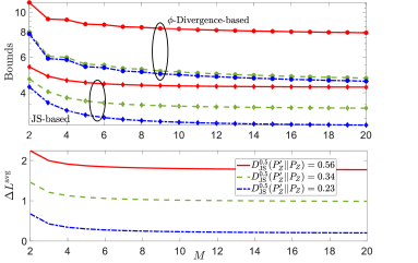
Figure 1: Average transfer generalization gap (16) (bottom) and the $(0.5,0.5)$-JS-based bound in (9) and $\phi$-divergence based bound in [1, Cor. 3] (top) as a function of $M$ (when $\beta=1$) for varying JS divergence between $P^{\prime}_{Z}$ and a fixed $P_{Z}$ with $p_{s}=0.48$.

In Figure 1, we compare the the average transfer generalization gap (16) with the conventional JS-divergence bound of (9) for $\alpha_{1}=\alpha_{2}=0.5$ and the $\phi$-divergence based bound in [1, Cor. 3] with $\phi(x)=|x-1|$, for the case when $\beta=1$ (i.e., only source-domain data set available for training) as a function of increasing values of $M$. For fixed $P_{Z}$ with $p_{s}=0.48$, we vary the JS-divergence by varying $p_{t}$. As predicted by our bound, the transfer generalization gap decreases with increase in the number of source-data samples $M$ available for training. However, there exists a non-vanishing generalization gap even at high $M$, which is a direct consequence of the domain shift. Moreover, a larger JS-divergence between $P_{Z}$ and $P^{\prime}_{Z}$ is predictive of a larger average transfer generalization gap. Finally, we show that JS-divergence based bounds outperform the $\phi$-divergence based bound in [1, Cor. 3] when $\beta=1$ at varying JS distances.

We now study the advantage of considering the general family of $(\alpha_{1},\alpha_{2})$-JS divergence over the JS divergence. Since the loss function is bounded, Assumption III.1 holds for mixture distribution $R^{\alpha_{1}}_{Z}$ for any $\alpha_{1}\in[0,1]$. Consequently, the bound in (8) can be tightened by optimizing over $\alpha_{1}$ and $\alpha_{2}$.

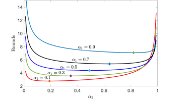
Figure 2: The $(\alpha_{1},\alpha_{2})$-JS divergence based bound in (8) as a function of $\alpha_{2}$ for varying $\alpha_{1}$ when $M=30$, $\beta=2/3$ and $\gamma=0.3$.

In Figure 2, we evaluate the tightness of the bound in (8) as a function of $\alpha_{2}$ for varying values of $\alpha_{1}$. As can be seen, the choice $(\alpha_{1}=0.1$, $\alpha_{2}\approx 0.2)$ yields the tightest bound. Therefore, the optimizing choice of $(\alpha_{1},\alpha_{2})$ does not result in existing JS divergences which assume $\alpha_{2}=0.5$ (symmetric skew JS divergence) or $\alpha_{2}=\alpha_{1}$ (asymmetric skew JS divergence).

Appendix A Proof of Theorem III.1

To obtain an upper bound on $\Delta L^{{\rm avg}}$, we use the decomposition (7) and separately bound the two differences. The average of the first difference in (7) can be equivalently written as $\mathbb{E}_{P_{Z^{M},W}}[L_{g}(W)-L_{t}(W|Z^{\beta M})]=$

$$\frac{1}{\beta M}\sum_{i=1}^{\beta M}\biggl{[}\mathbb{E}_{P_{W}P^{\prime}_{Z_{i}}}[l(W,Z_{i})]-\mathbb{E}_{P_{Z_{i}}P_{W|Z_{i}}}[l(W,Z_{i})]\biggr{]}$$ (17)

and similarly $\mathbb{E}_{P_{Z^{M},W}}[L_{g}(W)-L_{t}(W|Z^{(1-\beta)M})]=$

$$\frac{\sum_{i=\beta M+1}^{M}\biggl{[}\mathbb{E}_{P_{W}P^{\prime}_{Z_{i}}}[l(W,Z_{i})]-\mathbb{E}_{P^{\prime}_{Z_{i}}P_{W|Z_{i}}}[l(W,Z_{i})]\biggr{]}}{(1-\beta)M}.$$ (18)

We first bound the difference $\mathbb{E}_{P_{W}P^{\prime}_{Z_{i}}}[l(W,Z_{i})]-\mathbb{E}_{P_{Z_{i}}P_{W|Z_{i}}}[l(W,Z_{i})]$ in (17). Towards this, we use the exponential inequalities in Lemma A.1 obtained based on the change of measure approach adopted in [12]. Fix $\lambda=\lambda_{1}/\alpha_{2}$ for some $\lambda_{1}>0$ in (21) and $\lambda=-\lambda_{1}/(1-\alpha_{2})$ in (22), and apply Jensen’s inequality yield the following inequalities

$$\mathbb{E}_{P_{W}P^{\prime}_{Z_{i}}}[l(W,Z_{i})]-\mathbb{E}_{P_{W}R^{\alpha_{1}}_{Z}}[l(W,Z)]\leq\frac{\lambda_{1}\sigma^{2}}{2\alpha_{2}}$$

$$\quad+\frac{\alpha_{2}D_{{\rm KL}}(P^{\prime}_{Z}||R^{\alpha_{1}}_{Z})}{\lambda_{1}}$$ (19)

$$\mathbb{E}_{P_{W}R_{Z}^{\alpha_{1}}}[l(W,Z)]-\mathbb{E}_{P_{Z_{i}}P_{W|Z_{i}}}[l(W,Z_{i})]\leq\frac{\lambda_{1}\sigma^{2}}{2(1-\alpha_{2})}$$

$$\hskip 28.45274pt+\frac{1-\alpha_{2}}{\lambda_{1}}\biggl{(}D_{{\rm KL}}(P_{Z}||R^{\alpha_{1}}_{Z})+I(W;Z_{i})\biggr{)}.$$ (20)

Adding (19) and (20) and choosing

$$\lambda_{1}=\sqrt{\frac{D_{{\rm JS}}^{\alpha_{1},\alpha_{2}}(P^{\prime}_{Z}||P_{Z})+(1-\alpha_{1})I(W;Z_{i})}{\frac{\sigma^{2}}{2}\Bigl{(}\frac{1}{\alpha_{2}}+\frac{1}{1-\alpha_{2}}\Bigr{)}}}$$

gives that $\mathbb{E}_{P_{W}P^{\prime}_{Z_{i}}}[l(W,Z_{i})]-\mathbb{E}_{P_{Z_{i}}P_{W|Z_{i}}}[l(W,Z_{i})]\leq$

$$\sqrt{2\sigma^{2}\biggl{(}\frac{1}{\alpha_{2}}+\frac{1}{1-\alpha_{2}}\biggr{)}\biggl{(}D_{{\rm JS}}^{\alpha_{1},\alpha_{2}}(P^{\prime}_{Z}||P_{Z})+(1-\alpha_{2})I(W;Z_{i})\biggr{)}}.$$

Similarly, we can bound the difference $\mathbb{E}_{P_{W}P^{\prime}_{Z_{i}}}[l(W,Z_{i})]-\mathbb{E}_{P^{\prime}_{Z_{i}}P_{W|Z_{i}}}[l(W,Z_{i})]$ in (18) by fixing $\lambda=\lambda_{1}>0$ in (21) and $\lambda=-\lambda_{1}$ in (23). Applying Jensen’s inequality on both bounds, adding the resultant inequalities and choosing $\lambda_{1}=\sqrt{2D_{{\rm KL}}(P^{\prime}_{Z}||R^{\alpha_{1}}_{Z})+I(W;Z_{i})}/\sigma$ gives the corresponding bound.

Lemma A.1

Under Assumption III.1, the following inequalities hold for all $\lambda\in\mathbb{R}$ when $i=1,\ldots,\beta M$,

$$\mathbb{E}_{P_{W}P^{\prime}_{Z_{i}}}\biggl{[}\mathop{\hbox{\rm exp}}\biggl{(}\lambda(l(W,Z_{i})-\mathbb{E}_{P_{W}R_{Z}^{\alpha_{1}}}[l(W,Z)])-\frac{\lambda^{2}\sigma^{2}}{2}$$

$$\qquad-\log\frac{P^{\prime}_{Z_{i}}(Z_{i})}{R_{Z_{i}}^{\alpha_{1}}(Z_{i})}\biggr{)}\biggr{]}\leq 1,$$ (21)

$$\mathbb{E}_{P_{Z_{i}}P_{W|Z_{i}}}\biggl{[}\mathop{\hbox{\rm exp}}\biggl{(}\lambda(l(W,Z_{i})-\mathbb{E}_{P_{W}R_{Z}^{\alpha_{1}}}[l(W,Z)])-\frac{\lambda^{2}\sigma^{2}}{2}$$

$$\qquad-\log\frac{P_{Z_{i}}(Z_{i})}{R_{Z_{i}}^{\alpha_{1}}(Z_{i})}-\imath(W,Z_{i})\biggr{)}\biggr{]}\leq 1,$$ (22)

where $\imath(W,Z_{i})=\log(P_{W,Z_{i}}(W,Z_{i})/(P_{W}P_{Z_{i}}(W,Z_{i}))$ is the information density between random variables $W$ and $Z_{i}$. For $i=\beta M+1,\ldots,M$, the inequality (21) holds along with the following inequality

$$\mathbb{E}_{P^{\prime}_{Z_{i}}P_{W|Z_{i}}}\biggl{[}\mathop{\hbox{\rm exp}}\biggl{(}\lambda(l(W,Z_{i})-\mathbb{E}_{P_{W}R_{Z}^{\alpha_{1}}}[l(W,Z)])-\frac{\lambda^{2}\sigma^{2}}{2}$$

$$\qquad-\log\frac{P^{\prime}_{Z_{i}}(Z_{i})}{R_{Z_{i}}^{\alpha_{1}}(Z_{i})}-\imath(W,Z_{i})\biggr{)}\biggr{]}\leq 1.$$ (23)

Proof:

See Appendix B.  

Appendix B Proof of Lemma A.1

The derivation of the exponential inequalities leverage the change of measure approach adopted in [12]. For $i=1,\ldots,M$, Assumption III.1 gives that

$$\mathbb{E}_{P_{W}R^{\alpha_{1}}_{Z_{i}}}\biggl{[}\mathop{\hbox{\rm exp}}\biggl{(}\lambda(l(W,Z_{i})-\mathbb{E}_{P_{W}R_{Z}^{\alpha_{1}}}[l(W,Z)])-\frac{\lambda^{2}\sigma^{2}}{2}\biggr{)}\biggr{]}\leq 1.$$ (24)

For $i=1,\ldots,\beta M$, the inequality (24) implies the following inequality,

$$\mathbb{E}_{P_{W}R^{\alpha_{1}}_{Z_{i}}}\biggl{[}{\mathbb{I}}_{\mathcal{E}} \mathop{\hbox{\rm exp}}\biggl{(}\lambda(l(W,Z_{i})-\mathbb{E}_{P_{W}R_{Z}^{\alpha_{1}}}[l(W,Z)])-\frac{\lambda^{2}\sigma^{2}}{2}\biggr{)}\biggr{]}$$

$$\leq 1,$$ (25)

where $\mathcal{E}={\rm supp}(P^{\prime}_{Z_{i}})$, and ${\mathbb{I}}_{E}$ denotes the indicator function which takes value $1$ when the event $E$ is true, and is zero otherwise. Now, performing a change of measure from $R_{Z_{i}}^{\alpha_{1}}$ to $P^{\prime}_{Z_{i}}$ as in [13, Prop. 17] yields (21).

To get to inequality (22), we similarly first perform change of measure from $R^{\alpha_{1}}_{Z_{i}}$ to $P_{Z_{i}}$ on (24) to get the inequality

$$\mathbb{E}_{P_{W}P_{Z_{i}}}\biggl{[}\mathop{\hbox{\rm exp}}\biggl{(}\lambda(l(W,Z_{i})-\mathbb{E}_{P_{W}R_{Z}^{\alpha_{1}}}[l(W,Z)])-\frac{\lambda^{2}\sigma^{2}}{2}$$

$$\qquad-\log\frac{P_{Z_{i}}(Z_{i})}{R_{Z_{i}}^{\alpha_{1}}(Z_{i})}\biggr{)}\biggr{]}\leq 1.$$ (26)

The inequality (26) implies the following

$$\mathbb{E}_{P_{W}P_{Z_{i}}}\biggl{[}{\mathbb{I}}_{\mathcal{E}_{1}}\mathop{\hbox{\rm exp}}\biggl{(}\lambda(l(W,Z_{i})-\mathbb{E}_{P_{W}R_{Z}^{\alpha_{1}}}[l(W,Z)])-\frac{\lambda^{2}\sigma^{2}}{2}$$

$$\qquad-\log\frac{P_{Z_{i}}(Z_{i})}{R_{Z_{i}}^{\alpha_{1}}(Z_{i})}\biggr{)}\biggr{]}\leq 1,$$ (27)

where $\mathcal{E}_{1}={\rm supp}(P_{W,Z_{i}})$. Now performing a change of measure from $P_{Z_{i}}P_{W}$ to $P_{Z_{i}}P_{W|Z_{i}}$ as in [13, Prop. 17], and using the definition of information density $\imath(W,Z_{i})$ yields (22).

For $i=\beta M+1,\ldots,M$, (21) can be verified to hold as before. To get to inequality (23), we perform a change of measure on (21) from $P^{\prime}_{Z_{i}}P_{W}$ to $P^{\prime}_{Z_{i}}P_{W|Z_{i}}$ as explained before.

Appendix C Proof of Theorem III.3

To obtain the required bound in (14), we show that the term $\mathbb{E}_{P_{Z}}[l(w^{*},Z)]-\mathbb{E}_{P^{\prime}_{Z}}[l(w^{*},Z)]$ can be bounded by $\sqrt{2\sigma^{2}D^{\alpha_{1},\alpha_{2}}_{{\rm JS}}(P^{\prime}_{Z}||P_{Z})\hat{\alpha}_{2}}$, where $\hat{\alpha}_{2}=1/\alpha_{2}+1/(1-\alpha_{2})$. Towards this, note that the following exponential inequality holds under Assumption III.2 with $w=w^{*}$

$$\mathbb{E}_{R_{Z}^{\alpha_{1}}}\biggl{[}\mathop{\hbox{\rm exp}}\biggl{(}\lambda(l(w^{*},Z)-\mathbb{E}_{R_{Z}^{\alpha_{1}}}[l(w^{*},Z)])-\frac{\lambda^{2}\sigma^{2}}{2}\biggr{)}\biggr{]}\leq 1.$$ (28)

Denote $\delta l(w^{*}):=l(w^{*},Z)-\mathbb{E}_{R_{Z}^{\alpha_{1}}}[l(w^{*},Z]$. Now, performing change of measure from $R_{Z}^{\alpha_{1}}$ to $P^{\prime}_{Z}$, and from $R^{\alpha_{1}}_{Z}$ to $P_{Z}$ on (28) respectively as in Lemma A.1, yields the following inequalities

$$\mathbb{E}_{P^{\prime}_{Z}}\biggl{[}\mathop{\hbox{\rm exp}}\biggl{(}\lambda\delta l(w^{*})-\log\frac{P^{\prime}_{Z}(Z)}{R_{Z}^{\alpha_{1}}(Z)}-\frac{\lambda^{2}\sigma^{2}}{2}\biggr{)}\biggr{]}\leq 1,$$ (29)

$$\mathbb{E}_{P_{Z}}\biggl{[}\mathop{\hbox{\rm exp}}\biggl{(}\lambda\delta l(w^{*})-\log\frac{P_{Z}(Z)}{R_{Z}^{\alpha_{1}}(Z)}-\frac{\lambda^{2}\sigma^{2}}{2}\biggr{)}\biggr{]}\leq 1.$$ (30)

Take $\lambda=\lambda_{1}/\alpha_{2}$ for some $\lambda_{1}>0$ in (30) and $\lambda=-\lambda_{1}/(1-\alpha_{2})$ in (29). Now apply Jensen’s inequality on (29) and (30), and add the resulting inequalities to get the following inequality

$$\mathbb{E}_{P_{Z}}[l(w^{*},Z)]-L_{g}(w^{*})\leq\frac{\lambda_{1}\sigma^{2}\hat{\alpha}_{2}}{2}+\frac{1}{\lambda_{1}}D_{{\rm JS}}^{\alpha_{1},\alpha_{2}}(P^{\prime}_{Z}||P_{Z}).$$ (31)

Now, letting $\lambda_{1}=\sqrt{D_{{\rm JS}}^{\alpha_{1},\alpha_{2}}(P^{\prime}_{Z}||P_{Z})/(0.5\sigma^{2}\hat{\alpha}_{2})}$ yields the required bound.

Appendix D $(\alpha_{1},\alpha_{2})$-JS Divergence Based Bound for Loss Functions with Bounded CGF

Theorem D.1

Assume that the CGF of the loss function $l(W,Z)$ is upper bounded by a function $\Psi(\lambda)$ when $(W,Z)\sim P_{W}R^{\alpha}_{Z}$ for $\lambda\in[b_{-},b_{+}]$. Then, for $\beta\in(0,1)$ and $\alpha_{2}\in(0,1)$, the following upper bound on the average transfer generalization gap holds,

$$\Delta L^{{\rm avg}}\leq\frac{\gamma}{\beta M}\sum_{i=1}^{\beta M}\inf_{\lambda_{1}\in(0,b)}\biggl{(}\frac{1}{\lambda_{1}}\biggl{(}\widehat{\Psi}(\lambda_{1})+D_{{\rm JS}}^{\alpha_{1},\alpha_{2}}(P^{\prime}_{Z}||P_{Z})$$

$$+(1-\alpha_{2})I(W;Z_{i})\biggr{)}+\frac{1-\gamma}{(1-\beta)M}\sum_{i=\beta M+1}^{M}\inf_{\lambda_{2}\in(0,b_{2})}\biggl{(}\frac{1}{\lambda_{2}}\biggl{(}\Psi(\lambda_{2})$$

$$+\Psi(-\lambda_{2})+2D_{{\rm KL}}(P^{\prime}_{Z}||R_{Z}^{\alpha_{1}})+I(W;Z_{i})\biggr{)}\biggr{)},$$ (32)

where

$$\widehat{\Psi}(\lambda)=\alpha_{2}\Psi\Bigl{(}\frac{\lambda_{1}}{\alpha_{2}}\Bigr{)}+(1-\alpha_{2})\Psi\Bigl{(}\frac{-\lambda_{1}}{1-\alpha_{2}}\Bigr{)},$$

$b=\min\{\alpha_{2}b_{+},-(1-\alpha_{2})b_{-}\}$ and $b_{2}=\min\{b_{+},-b_{-}\}$.

Proof:

The assumption that the CGF of the loss function is bounded by $\Psi(\lambda)$ implies the following inequality for $i=1,\ldots,M$

$$\mathbb{E}_{P_{W}R^{\alpha}_{Z_{i}}}\biggl{[}\mathop{\hbox{\rm exp}}\biggl{(}\lambda(l(W,Z_{i})-\mathbb{E}_{P_{W}R_{Z}^{\alpha}}[l(W,Z)])-\Psi(\lambda)\biggr{)}\biggr{]}\leq 1,$$ (33)

for all $\lambda\in[b_{-},b_{+}]$. It is then easy to see that the exponential inequalities in Lemma A.1 hold with the term $\lambda^{2}\sigma^{2}/2$ replaced by $\Psi(\lambda)$.

Now, proceed as in the proof of Theorem III.1 in Appendix A to bound the difference $\mathbb{E}_{P_{W}P^{\prime}_{Z}}[l(W,Z)]-\mathbb{E}_{P_{Z_{i}}P_{W|Z_{i}}}[l(W,Z_{i})]$. This results in the following inequalities replacing (19) and (20)

$$\mathbb{E}_{P_{W}P^{\prime}_{Z_{i}}}[l(W,Z_{i})]-\mathbb{E}_{P_{W}R^{\alpha_{1}}_{Z}}[l(W,Z)]$$

$$\leq\frac{\alpha_{2}}{\lambda_{1}}\biggl{(}\Psi\Bigl{(}\frac{\lambda_{1}}{\alpha_{2}}\Bigr{)}+D_{{\rm KL}}(P^{\prime}_{Z}||R^{\alpha_{1}}_{Z})\biggr{)}$$ (34)

$$\mathbb{E}_{P_{W}R_{Z}^{\alpha_{1}}}[l(W,Z)]-\mathbb{E}_{P_{Z_{i}}P_{W|Z_{i}}}[l(W,Z_{i})]$$

$$\leq\frac{1-\alpha_{2}}{\lambda_{1}}\biggl{(}\Psi\Bigl{(}\frac{-\lambda_{1}}{1-\alpha_{2}}\Bigr{)}+D_{{\rm KL}}(P^{\prime}_{Z}||R^{\alpha_{1}}_{Z})+I(W;Z_{i})\biggr{)},$$ (35)

which holds for all $\lambda_{1}\in(0,\min\{\alpha_{2}b_{+},-(1-\alpha_{2})b_{-})$. Adding (34) and (35), and subsequently optimizing over $\lambda_{1}$ yields the required bound on $\mathbb{E}_{P_{W}P^{\prime}_{Z}}[l(W,Z)]-\mathbb{E}_{P_{Z_{i}}P_{W|Z_{i}}}[l(W,Z_{i})]$.

To bound the difference $\mathbb{E}_{P_{W}P^{\prime}_{Z}}[l(W,Z)]-\mathbb{E}_{P^{\prime}_{Z_{i}}P_{W|Z_{i}}}[l(W,Z_{i})]$, we proceed as in Appendix A by fixing $\lambda=\lambda_{2}$ in (21) and $\lambda=-\lambda_{2}$ in (23) with $\lambda^{2}\sigma^{2}/2$ replaced by $\Psi(\lambda)$, for $\lambda_{2}\in(0,\min\{-b_{-},b_{+}\})$. This results in the following bound

$$\mathbb{E}_{P_{W}P^{\prime}_{Z}}[l(W,Z)]-\mathbb{E}_{P^{\prime}_{Z_{i}}P_{W|Z_{i}}}[l(W,Z_{i})]\leq$$

$$\frac{1}{\lambda_{2}}\biggl{(}\Psi(\lambda_{2})+\Psi(-\lambda_{2})+2D_{{\rm KL}}(P^{\prime}_{Z}||R^{\alpha_{1}}_{Z})+I(W;Z_{i})\biggr{)}.$$ (36)

Now optimizing over $\lambda_{2}\in(0,\min\{-b_{-},b_{+}\})$ yields the required bound.  

We now specialize the bound in (32) to the case of sub-gamma loss function.

Corollary D.2

Assume that the loss function $l(W,Z)$ is sub-gamma with variance parameter $\sigma$ and scale parameter $c$ such that its CGF is upper bounded by $\Psi(\lambda)=\lambda^{2}\sigma^{2}/2(1-c|\lambda|)$ for $|\lambda|<1/c$. Then, the following upper bound holds for the average transfer generalization gap when $\beta\in(0,1)$ and $\alpha_{2}=0.5$,

$$\Delta L^{{\rm avg}}\leq\frac{\gamma}{\beta M}\sum_{i=1}^{\beta M}\biggl{(}2\sqrt{2\sigma^{2}(D_{{\rm JS}}^{\alpha_{1},0.5}(P^{\prime}_{Z}||P_{Z})+0.5I(W;Z_{i}))}$$

$$+2c\sqrt{2\sigma^{2}(D_{{\rm JS}}^{\alpha_{1},0.5}(P^{\prime}_{Z}||P_{Z})+0.5I(W;Z_{i})}\biggr{)}+$$

$$\frac{1-\gamma}{(1-\beta)M}\sum_{i=\beta M+1}^{M}\biggl{(}2\sqrt{\sigma^{2}(2D_{{\rm KL}}(P^{\prime}_{Z}||R_{Z}^{\alpha_{1}})+I(W;Z_{i}))}$$

$$+c(2D_{{\rm KL}}(P^{\prime}_{Z}||R_{Z}^{\alpha_{1}})+I(W;Z_{i})).\biggr{)}$$ (37)

Proof:

The proof follows from (32) where the optimizing $\lambda_{1}$ is given as

$$\frac{\sqrt{D_{{\rm JS}}^{\alpha_{1},\alpha_{2}}(P^{\prime}_{Z}||P_{Z})+I(W;Z_{i})}}{\sqrt{2\sigma^{2}}+2c\sqrt{D_{{\rm JS}}^{\alpha_{1},\alpha_{2}}(P^{\prime}_{Z}||P_{Z})+I(W;Z_{i})}}\in(0,\frac{1}{2c})$$

and the optimizing $\lambda_{2}$ corresponds to

$$\lambda_{2}=\frac{\sqrt{2D_{{\rm KL}}(P^{\prime}_{Z}||R_{Z}^{\alpha_{1}})+I(W;Z_{i})}}{\sigma+\sqrt{2D_{{\rm KL}}(P^{\prime}_{Z}||R_{Z}^{\alpha_{1}})+I(W;Z_{i})}}\in(0,\frac{1}{c}).$$

References

[1]
X. Wu, J. H. Manton, U. Aickelin, and J. Zhu, “Information-theoretic analysis
for transfer learning,” arXiv preprint arXiv:2005.08697, 2020.
[2]
L. Torrey and J. Shavlik, “Transfer learning,” in Handbook of research
on machine learning applications and trends: algorithms, methods, and
techniques. IGI global, 2010, pp.
242–264.
[3]
S. Ben-David, J. Blitzer, K. Crammer, and F. Pereira, “Analysis of
Representations for Domain Adaptation,” in Advances in Neural
Information Processing Systems, 2007, pp. 137–144.
[4]
S. Ben-David, J. Blitzer, K. Crammer, A. Kulesza, F. Pereira, and J. W.
Vaughan, “A theory of learning from different domains,” Machine
Learning, vol. 79, no. 1-2, pp. 151–175, 2010.
[5]
Y. Mansour, M. Mohri, and A. Rostamizadeh, “Domain Adaptation: Learning
Bounds and Algorithms,” arXiv preprint arXiv:0902.3430, 2009.
[6]
C. Zhang, L. Zhang, and J. Ye, “Generalization Bounds for Domain
Adaptation,” in Advances in Neural Information Processing
Systems, 2012, pp. 3320–3328.
[7]
F. Nielsen, “On a generalization of the Jensen–Shannon divergence and the
Jensen–Shannon centroid,” Entropy, vol. 22, no. 2, p. 221, 2020.
[8]
T. Yamano, “Some bounds for skewed -Jensen-Shannon divergence,”
Results in Applied Mathematics, vol. 3, p. 100064, 2019.
[9]
C. Shui, Q. Chen, J. Wen, F. Zhou, C. Gagné, and B. Wang, “Beyond
-divergence: domain adaptation theory with Jensen-Shannon
divergence,” arXiv preprint arXiv:2007.15567, 2020.
[10]
A. Xu and M. Raginsky, “Information-Theoretic Analysis of Generalization
Capability of Learning Algorithms,” in Proc. of Adv. in Neural
Inf. Processing Sys. (NIPS), Dec. 2017, pp. 2524–2533.
[11]
Y. Bu, S. Zou, and V. V. Veeravalli, “Tightening mutual information based
bounds on generalization rrror,” in Proc. of IEEE Int. Symp. Inf.
Theory (ISIT), July 2019, pp. 587–591.
[12]
F. Hellström and G. Durisi, “Generalization bounds via information density
and conditional information density,” arXiv preprint
arXiv:2005.08044, 2020.
[13]
Y. Polyanskiy and Y. Wu, “Lecture notes on information theory,” Lecture
Notes for ECE563 (UIUC), vol. 6, no. 2012-2016, p. 7, 2014.