$\ell_{2}$-Relaxation: With Applications to
Forecast Combination and Portfolio Analysis

Abstract

This paper tackles forecast combination with many forecasts or minimum variance portfolio selection with many assets. A novel convex problem called $\ell_{2}$-relaxation is proposed. In contrast to standard formulations, $\ell_{2}$-relaxation minimizes the squared Euclidean norm of the weight vector subject to a set of relaxed linear inequality constraints. The magnitude of relaxation, controlled by a tuning parameter, balances the bias and variance. When the variance-covariance (VC) matrix of the individual forecast errors or financial assets exhibits latent group structures — a block equicorrelation matrix plus a VC for idiosyncratic noises, the solution to $\ell_{2}$-relaxation delivers roughly equal within-group weights. Optimality of the new method is established under the asymptotic framework when the number of the cross-sectional units $N$ potentially grows much faster than the time dimension $T$. Excellent finite sample performance of our method is demonstrated in Monte Carlo simulations. Its wide applicability is highlighted in three real data examples concerning empirical applications of microeconomics, macroeconomics, and finance.

Key Words: Forecast combination puzzle; high dimension; latent group; machine learning; portfolio analysis; optimization.

JEL Classification: C22, C53, C55

We thank the editor and two referees for their valuable suggestions. We are also grateful to Bruce Hansen, Yingying Li, Esfandiar Maasoumi, Jack Porter, Yuying Sun, Aman Ullah, Xia Wang, Xinyu Zhang, and Xinghua Zheng for their helpful comments. Shi acknowledges financial support from Hong Kong Research Grants Council (RGC) No.14500118. Su gratefully acknowledges the support from Natural Science Foundation of China (No.72133002). Xie’s research is supported by the Natural Science Foundation of China (No.72173075), the Shanghai Research Center for Data Science and Decision Technology, and the Fundamental Research Funds for the Central Universities. Address correspondence: Zhentao Shi: zhentao.shi@gatech.edu, School of Economics, Georgia Institute of Technology, 205 Old C.E. Building, 221 Bobby Dodd Way, Atlanta, GA 30332, U.S.A., and Department of Economics, 928 Esther Lee Building, the Chinese University of Hong Kong, Shatin, New Territories, Hong Kong SAR, China. Liangjun Su: sulj@sem.tsinghua.edu.cn, School of Economics and Management, Tsinghua University, Beijing, China. Tian Xie: xietian@shufe.edu.cn, College of Business, Shanghai University of Finance and Economics, Shanghai, China.

1 Introduction

Forecast combination assigns weights to individual experts to reduce forecast errors, and portfolio management assigns weights to financial assets to reduce risk exposure. The classical approach to both problems, to be formally laid out in Section 2.1, solves a quadratic optimization

$$\min_{\mathbf{w}\in\mathbb{R}^{N}}\,\frac{1}{2}\mathbf{w}^{\prime}\widehat{\boldsymbol{\Sigma}}\mathbf{w}\ \ \text{subject to \ }\mathbf{w}^{\prime}\boldsymbol{1}_{N}=1,$$ (1.1)

where $N$ is the number of forecasts or assets, $\mathbf{1}_{N}$ is a column of $N$ ones, and $\widehat{\boldsymbol{\Sigma}}$ is a variance-covariance (VC) matrix estimate computed from $T$ time series observations. When $\widehat{\boldsymbol{\Sigma}}$ is invertible, the explicit solution to (1.1) is

$$\widehat{\mathbf{w}}^{\mathrm{\mathrm{C}}}=(\boldsymbol{1}_{N}^{\prime}\widehat{\boldsymbol{\Sigma}}^{-1}\boldsymbol{1}_{N})^{-1}\widehat{\boldsymbol{\Sigma}}^{-1}\boldsymbol{1}_{N},$$ (1.2)

where “C” in the superscript refers to the classical approach.

Consider, for simplicity, the case when $\widehat{\boldsymbol{\Sigma}}$ is estimated as the plain sample VC matrix computed from $T$ observations of $N\times 1$ vectors, where each entry represents a forecast error in forecast combination (Bates and Granger, 1969), or an asset’s excess return in a portfolio (Markowitz, 1952). When $T\gg N$, the classical solution (1.2) is valid as $\widehat{\boldsymbol{\Sigma}}$ is generally invertible. However, $\widehat{\boldsymbol{\Sigma}}$ may suffer ill-posedness when $N$ is comparable to $T$, and it is singular when $N$ is larger than $T$, which invalidates (1.2). Such defects are well recognized in the empirical literature. When $N$ is large, $\widehat{\mathbf{w}}^{\mathrm{C}}$ often performs poorly because of the difficulty in estimating the large population VC matrix with precision. Rather, the simple average (namely, equal-weight) routinely outperforms. In forecast combination, this empirical fact is known as the forecast combination puzzle (Clemen, 1989; Stock and Watson, 2004). Parallelly, in portfolio management the so-called naive $1/N$ diversification strategy is found to achieve robust out-of-sample gains compared to many sophisticated alternatives (DeMiguel et al., 2009; DeMiguel et al., 2009).

In this paper, we propose a new estimation technique on the weights, to be presented in Section 2.2 below. This method minimizes the squared Euclidean norm ($\ell_{2}$-norm) of the weight vector subject to a relaxed version of the first order conditions from the minimization problem in (1.1), yielding the $\ell_{2}$-relaxation problem. The strategy is similar in spirit to the $\ell_{1}$-relaxation in Dantzig selector a la Candes and Tao (2007). Interestingly,  $\ell_{2}$-relaxation incorporates as special cases the simple average (equal-weight) strategy by setting the tuning parameter to be sufficiently large, and the classical optimal weighting scheme when the tuning parameter is zero. The tuning parameter helps to balance the bias and variance and to deliver roughly equal groupwise weights when the VC matrix exhibits a certain latent group structure. This is consistent with the intuition that when the VC matrix displays an exactly block equicorrelation structure, one should assign the same weight to all individual units within the same group whereas potentially distinct weights to the units in different groups. When the VC matrix is contaminated with a noise component, we show that the resultant $\ell_{2}$-relaxed weights are close to the infeasible groupwise equal weights.

The approximate latent group structure is not a man-made artifact. It is inherent in many models and applications. For example, it emerges when a factor structure dwells in the forecasting errors and the factor loadings are directly governed by certain latent group structures or are approximable by a few values (see Examples 1 and 2 in Section 3.1). It emerges when forecast combinations are based on a large number of forecast models with a fixed number of predictive regressors (see Example 3 in Section 3.1). It also emerges when industrial classification serves as a proxy of the clustering pattern in the VC matrix of returns of stocks (see Example 5 in Section 3.1).

Given the latent group structure, we establish two main theoretical results under a high dimensional asymptotic framework in which the number of individual units can be much larger than the time series dimension. (i) The estimated weights of $\ell_{2}$-relaxation converges to the within-group equal-weight solution (see Theorem 1 in Section 3.2), and (ii) The empirical risk based on $\ell_{2}$-relaxation approaches the risk given by the oracle group information (see Theorem 2 in Section 3.2). We assess the finite sample behavior of $\ell_{2}$-relaxation in Monte Carlo simulations. Compared with the oracle estimator and some popular off-the-shelf machine learning estimators, $\ell_{2}$-relaxation performs well under various data generating processes (DGPs). We further evaluate its empirical accuracy in three real data examples covering box office prediction, inflation forecast by surveyed professionals, and financial market portfolios. These examples showcase the wide applicability of $\ell_{2}$-relaxation.

Literature Review. This paper stands on several strands of vast literature. Forecast combination is reviewed by Clemen (1989) and Elliott and Timmermann (2016) up to the points of their writing. Averaging forecasts appear to be a more robust procedure than the so-called optimal combination (Bates and Granger, 1969), and a reasonable explanation suggests that the errors on the estimation of the weights can be large and thus dominate the gains from the use of optimal combination (see, e.g., Smith and Wallis, 2009, Claeskens et al., 2016).

A lesson learned from this literature is that it is unwise to include all possible variables; limiting the number of unknown parameters can help reduce estimation errors. This stylized fact has catalyzes the adoption of various shrinkage, regularization, and machine learning techniques. See, e.g., Hansen (2007), Conflitti et al. (2015), Bayer (2018), Wilms et al. (2018), Kotchoni et al. (2019), Coulombe et al. (2020), Diebold et al. (2022), and Roccazzella et al. (2020). In particular, Elliott et al. (2013) propose a complete subset regression (CSR) approach to forecast combinations by using equal weights to combine forecasts based on the same number of predictive variables. Diebold and Shin (2019) bring forth the partially egalitarian Lasso (peLASSO) procedures that discard some forecasts and then shrink the remaining forecasts toward the equal weights. Our $\ell_{2}$-relaxation adds a new way to regularize the weight estimation and includes the strategy of Diebold and Shin (2019) as a special case.

Our paper is related to the burgeoning literature on latent group structures in panel data analysis; see, e.g., Bonhomme and Manresa (2015), Su et al. (2016), Su and Ju (2018), Su et al. (2019), Vogt and Linton (2017), Vogt and Linton (2020), and Bonhomme et al. (2022). While most of these previous studies focus on the recovery of the latent group structures in the conditional mean model, in our paper the group pattern is a latent structure in the VC matrix that encourages parameter parsimony and facilitates estimation accuracy. We do not attempt to recover the group identities.

Lastly, there is statistical and financial econometric literature on the estimation of large VC matrix. See Disatnik and Katz (2012), Fan et al. (2012), Fan et al. (2013), Fan et al. (2016), Ledoit and Wolf (2017), and Ao et al. (2019), among many others. In particular, Ledoit and Wolf (2004) use Bayesian methods for shrinking the sample correlation matrix to an equicorrelated target and show that this helps select portfolios with low volatility compared to those based on the sample correlation; Ledoit and Wolf (2017) promote a nonlinear shrinkage estimator that is more flexible than the previous linear shrinkage estimators. Instead of regularizing the VC matrix, $\ell_{2}$-relaxation shrinks the weights and it can be used in conjunction with a high dimensional VC estimator.

Our paper complements the literature from the following aspects. Firstly, in terms of combination techniques, we corroborate in theory and in numerical experiments that $\ell_{2}$-relaxation is a competitive and easy-to-implement procedure. Secondly, unlike most panel data group structure papers, we focus on improvement of the out-of-sample performance and do not attempt to recover the membership for each individual, and a latent community or group structure is assumed for statistical optimality. Finally, while the dominating method in the large scale portfolio analysis shrinks the entries of the VC matrix, we take a viable alternative to directly discipline the weights. In summary, within the unified framework of forecast combination and portfolio optimization, $\ell_{2}$-relaxation is an innovative method with asymptotic guarantee under latent group structures.

Organization. The rest of the paper is organized as follows. Section 2 motivates and introduces the $\ell_{2}$-relaxation problem. Section 3 studies the statistical properties of the estimator and establishes its asymptotic optimality under the latent group structures. Section 4 reports Monte Carlo simulation results. The new method is applied to three datasets in Section 5. All theoretical results are proved in Appendix A, and additional numerical results are contained in Appendix B.

Notation. Let “$:=$” signify a definition, “$\otimes$” be the Kronecker product, and $a\wedge b=\min\left\{a,b\right\}$. We write $a\asymp b$ when both $a/b$ and $b/a$ are stochastically bounded. For a random variable $x$, we write its population mean as $E\left[x\right]$; for a sample $\left(x_{1},\ldots,x_{T}\right)$, we write its sample mean as $\mathbb{E}_{T}\left[x_{t}\right]:=T^{-1}\sum_{t=1}^{T}x_{t}$. A plain $b$ denotes a scalar, a boldface lowercase $\mathbf{b}$ denotes a vector, and a boldface uppercase $\mathbf{B}$ denotes a matrix. The $\ell_{1}$-norm and $\ell_{2}$-norm of $\mathbf{b}=(b_{1},...,b_{n})^{\prime}$ are written as $\left\|\mathbf{b}\right\|_{1}:=\sum_{i=1}^{n}\left|b_{i}\right|$ and $\left\|\mathbf{b}\right\|_{2}:=\left(\sum_{i=1}^{n}b_{i}^{2}\right)^{1/2},$ respectively. For a generic index set $\mathcal{G}\subset\left[N\right]:=\left\{1,\ldots,N\right\}$, we denote $\left|\mathcal{G}\right|$ as the cardinality of $\mathcal{G}$, and $\mathbf{b}_{\mathcal{G}}=\left(b_{i}\right)_{i\in\mathcal{G}_{k}}$ as the $\left|\mathcal{G}\right|$-dimensional subvector. $\phi_{\max}\left(\mathbf{\cdot}\right)$ and $\phi_{\min}\left(\cdot\right)$ represent the maximum and minimum eigenvalues of a real symmetric matrix, respectively. For a generic $n\times m$ matrix $\mathbf{B}$, define the sup-norm as $\left\|\mathbf{B}\right\|_{\infty}:=\max_{i\leq n,j\leq m}\left|b_{ij}\right|$, and the maximum column $\ell_{2}$ matrix norm as $\left\|\mathbf{B}\right\|_{c2}:=\max\nolimits_{j\leq m}\|\mathbf{B}_{\cdot j}\|_{2}$, where $\mathbf{B}_{\cdot j}$ is the $j$-th column. $\boldsymbol{0}_{n}$ and $\boldsymbol{1}_{n}$ are $n\times 1$ vectors of zeros and ones, respectively, and $\mathbf{\mathbf{I}}_{n}$ is the $n\times n$ identity matrix.

2 Formulation

2.1 Classical Approaches

In this section, we fix the ideas by characterizing the similarities between the classical forecast combination problem and portfolio optimization. We start with the former. Suppose that $y_{t+1}$ is an outcome variable, and there are $N$ forecasts for $y_{t+1}$, stacked as $\mathbf{f}_{t}=(f_{1t},...,f_{Nt})^{\prime}$, available at time $t$. The time dimension is indexed by $t\in\left[T\right]:=\{1,2,...,T\}$, and the cross-sectional units are indexed by $i\in\left[N\right]$. An $N\times 1$ weight vector $\mathbf{w}=(w_{i})_{i\in[N]}$ will linearly combine the forecasts into $\mathbf{w}^{\prime}\mathbf{f}_{t}$. We are interested in finding the weight $\mathbf{w}$ to minimize the mean squared forecast error (MSFE) of the combined forecast error $(y_{t+1}-\mathbf{w}^{\prime}\mathbf{f}_{t})$.

We collect the individual forecast error $e_{it}:=y_{t+1}-f_{it}$, and denote $\mathbf{e}_{t}:=(e_{it})_{i\in[N]}$ and $\bar{\mathbf{e}}:=T^{-1}\sum_{t=1}^{T}\mathbf{e}_{t}$. We compute its plain sample VC matrix

$$\widehat{\boldsymbol{\Sigma}}:=T^{-1}\sum_{t=1}^{T}(\mathbf{e}_{t}-\bar{\mathbf{e}})(\mathbf{e}_{t}-\bar{\mathbf{e}})^{\prime}.$$ (2.1)

Traditionally, the weights are determined by solving (1.1).

Forecast combination is intrinsically related to the mean-variance analysis of portfolio selection (Markowitz, 1952). Given $N$ financial assets of excess (relative to a risk-free asset) return $\mathbf{r}_{t}=(r_{it})_{i\in[N]}$, write the sample average return $\bar{\mathbf{r}}:=T^{-1}\sum_{t=1}^{T}\mathbf{r}_{t}$ and the plain sample VC matrix

$$\widehat{\boldsymbol{\Sigma}}:=T^{-1}\sum_{t=1}^{T}(\mathbf{r}_{t}-\bar{\mathbf{r}})(\mathbf{r}_{t}-\bar{\mathbf{r}})^{\prime}.$$ (2.2)

The weight vector $\mathbf{w}$ can be solved from

$$\min_{\mathbf{w}\in\mathbb{R}^{N}}\,\frac{1}{2}\mathbf{w}^{\prime}\widehat{\boldsymbol{\Sigma}}\mathbf{w}\ \ \text{subject to \ }\mathbf{w}^{\prime}\boldsymbol{1}_{N}=1\mbox{ and }\bar{\mathbf{r}}^{\prime}\mathbf{w}\geq r^{\ast},$$ (2.3)

where $r^{\ast}$ is a user-specified target return. It is recognized that when there are many assets, precise estimation of the mean returns is a challenging task (Merton, 1980), and the recent literature shifts to the minimum variance portfolio (MVP). MVP drops the linear restriction on returns (i.e., $\bar{\mathbf{r}}^{\prime}\mathbf{w}\geq r^{\ast}$), which leads to an optimization problem identical to (1.1).

As forecast combination and MVP share the same form, we focus on the optimization problem in (1.1). It can be rewritten as an unconstrained Lagrangian problem $\mathbf{w}^{\prime}\widehat{\boldsymbol{\Sigma}}\mathbf{w}/2+\gamma\left(\mathbf{w}^{\prime}\boldsymbol{1}_{N}-1\right),$ where $\gamma$ is the Lagrangian multiplier. The corresponding Kuhn-Karush-Tucker (KKT) conditions are:

$$\begin{array}[]{rcl}\widehat{\boldsymbol{\Sigma}}\mathbf{w}+\gamma\boldsymbol{1}_{N}&=&\boldsymbol{0}_{N},\\ \mathbf{w}^{\prime}\boldsymbol{1}_{N}-1&=&0.\end{array}$$ (2.4)

The invertibility of the estimated VC matrix is not innocuous in high dimensional settings. For example, when $\widehat{\boldsymbol{\Sigma}}$ is the plain sample VC matrix, it must be singular when $N>T.$ Consider the case where $N$ is of similar magnitude to $T$ but $N<T$. Even if $\widehat{\boldsymbol{\Sigma}}$ is non-singular, a few sample eigenvalues of $\widehat{\boldsymbol{\Sigma}}$ are likely to be close to zero, leading to a numerically unstable solution when taking the matrix inverse in (1.2).

2.2 Relaxation

To stabilize the numerical solution, we are inspired by the Dantzig selector (Candes and Tao, 2007) and the relaxed empirical likelihood (Shi, 2016) to consider relaxing the sup-norm of the KKT condition as follows:

$$\min_{\left(\mathbf{w},\gamma\right)\in\mathbb{R}^{N+1}}\ \frac{1}{2}\left\|\mathbf{w}\right\|_{2}^{2}\text{ \ \ subject to \ }\mathbf{w}^{\prime}\boldsymbol{1}_{N}=1\ \text{and }\|\widehat{\boldsymbol{\Sigma}}\mathbf{w}+\gamma\boldsymbol{1}_{N}\|_{\infty}\leq\tau,$$ (2.5)

where $\tau$ is a tuning parameter to be specified by the user. We call the programming in (2.5) the $\ell_{2}$-relaxation problem, and denote its solution as $\widehat{\mathbf{w}}=\widehat{\mathbf{w}}_{\tau},$ where the dependence of $\widehat{\mathbf{w}}$ on $\tau$ is often suppressed for notational conciseness.

When $\tau=0$, the solution $\widehat{\mathbf{w}}$ is characterized by the KKT conditions in (2.4), and $\widehat{\mathbf{w}}^{\mathrm{C}}$ in (1.2) is the unique solution when $\widehat{\boldsymbol{\Sigma}}$ is invertible. Thus $\ell_{2}$-relaxation keeps the classical approach as a special case. Constraints in (2.5) are feasible for any $\tau\geq 0$. The solution to (2.5) is always unique because the objective is a strictly convex function and the feasible set is a closed convex set. The tuning parameter $\tau$ plays a crucial role in balancing the bias and variance: the bias is small when $\tau$ is small, whereas the variance is small when $\tau$ is large. If $\tau$ is sufficiently large, say $\tau\geq\max_{i\in\left[N\right]}|\widehat{\boldsymbol{\Sigma}}_{i\cdot}\boldsymbol{1}_{N}|/N$, the second constraint in (2.5) is slack and thus irrelevant to the minimization. As a result, the simple average weight $N^{-1}\boldsymbol{1}_{N}$ solves (2.5). In addition, relaxing $\tau$ from 0 reduces the sensitivity of the weights to the noise in the estimated VC matrix to prevent in-sample over-fitting.

On the other hand, $\ell_{2}$-relaxation can be motivated from the information theory as in Diebold et al. (2022). The choice of $\ell_{2}$-norm can be viewed as a special case of Rényi’s cross-entropy (Rényi, 1961, Eq.(1.21) with $\alpha=2$). This particular choice is for convenience because: (i) the dual of the Euclidean norm with respect to the inner product is the Euclidean norm itself and (ii) it accommodates $w_{i}<0$, which should not be ruled out in applications of forecast combination and portfolio analysis. By choosing a positive value of $\tau,$ the constraints in (2.5) yield a feasible set that is larger than that associated with $\tau=0.$ Let $\overline{w}:=\frac{1}{N}\sum_{i=1}^{N}w_{i}.$ Then

$$\left\|\mathbf{w}\right\|_{2}^{2}=\sum_{i=1}^{N}w_{i}^{2}=\sum_{i=1}^{N}\left(w_{i}-\bar{w}\right)^{2}+N\bar{w}^{2}=\sum_{i=1}^{N}\left(w_{i}-\frac{1}{N}\right)^{2}+\frac{1}{N},$$

where the last equality holds under the constraint $\mathbf{w}^{\prime}\boldsymbol{1}_{N}=1.$ Clearly, the $\ell_{2}$-relaxation aims to minimize the sample variance of the weights over the feasible set and it effectively eliminates unnecessary variations across the individual weights. As we shall see, in the presence of a latent group structure in the dominant component of the VC matrix, the $\ell_{2}$-relaxation shrinks the individual weights to the group mean. This allows our estimator to include the widely used simple average (SA) estimator as a special case.

3 Theoretical Analysis

3.1 Latent Group Structures

In this section, we impose latent group structures on $\widehat{\boldsymbol{\Sigma}}$ or its population expectation $E[\widehat{\boldsymbol{\Sigma}}]$ and then study the implications on the $\ell_{2}$-relaxed estimates of the weights.

Statistical analysis of high dimensional problems typically postulates certain structures on the data generating process for dimension reduction. For example, variable selection methods such as Lasso (Tibshirani, 1996) and SCAD (Fan and Li, 2001) are motivated from regressions with sparsity, meaning most of the regression coefficients are either exactly zero or approximately zero. Similarly, in large VC estimation, various structures have been considered in the literature. Bickel and Levina (2008) impose many off-diagonal elements to be zero, Engle and Kelly (2012) assume a block equicorrelation structure, and Ledoit and Wolf (2004) use Bayesian methods for shrinking the sample correlation matrix to an equicorrelated target, to name just a few.

Imposing latent group structures is an alternative way to reduce dimensions, which now has grown into a burgeoning literature. To analyze (2.5) in depth in the high dimensional framework, we assume $\widehat{\boldsymbol{\Sigma}}=\{\widehat{\Sigma}_{ij}\}_{i,j\in\left[N\right]}$ can be approximated by a block equicorrelation matrix:

$$\widehat{\boldsymbol{\Sigma}}=\widehat{\boldsymbol{\Sigma}}^{\ast}+\widehat{\boldsymbol{\Sigma}}^{e},$$ (3.1)

where $\widehat{\boldsymbol{\Sigma}}^{\ast}=\{\widehat{\Sigma}_{ij}^{\ast}\}_{i,j\in\left[N\right]}$ is a block equicorrelation matrix and $\widehat{\boldsymbol{\Sigma}}^{e}=\{\widehat{\Sigma}_{ij}^{e}\}_{i,j\in\left[N\right]}$ denotes the deviation of $\widehat{\boldsymbol{\Sigma}}$ from the block equicorrelation matrix. We write

$$\underset{\left(N\times N\right)}{\widehat{\boldsymbol{\Sigma}}^{\ast}}=\underset{\left(N\times K\right)}{\mathbf{Z}}\underset{\left(K\times K\right)}{\widehat{\mathbf{\Sigma}}^{\mathrm{co}}}\mathbf{Z}^{\prime}$$ (3.2)

where $\mathbf{Z}=\{Z_{ik}\}$ denotes an $N\times K$ binary matrix providing the cluster membership of each individual forecast, i.e., $Z_{ik}=1$ if forecast $i$ belongs to group $\mathcal{G}_{k}\subset\left[N\right]$ and $Z_{ik}=0$ otherwise, and $\widehat{\boldsymbol{\Sigma}}^{\mathrm{co}}=\{\widehat{\Sigma}_{kl}^{\mathrm{co}}\}_{k,l\in\left[K\right]}$ is a $K\times K$ symmetric positive definite matrix. Here, the superscript “co” stands for “core”. Note that $\widehat{\Sigma}_{ij}^{\ast}=\widehat{\Sigma}_{kl}^{\mathrm{co}}$ if $i\in\mathcal{G}_{k}\text{ and }j\in\mathcal{G}_{l}.$

One can observe $\widehat{\boldsymbol{\Sigma}}$ from the data but not $\widehat{\boldsymbol{\Sigma}}^{\ast}$. We will be precise about the definition of “approximation” for $\widehat{\boldsymbol{\Sigma}}^{e}$ in Assumption 1 later. Let $N_{k}:=\left|\mathcal{G}_{k}\right|$ be the number of individuals in the $k$th group, and thus $N=\sum_{k=1}^{K}N_{k}$. For ease of notation and after necessary re-ordering the $N$ forecast units, we write

$$\widehat{\boldsymbol{\Sigma}}^{\ast}=(\widehat{\Sigma}_{kl}^{\mathrm{co}}\cdot\boldsymbol{1}_{N_{k}}\boldsymbol{1}_{N_{l}}^{\prime})_{k,l\in[K],}$$ (3.3)

in which the units in the same group cluster together in a block. The re-ordering is for the convenience of notation only. The theory to be developed is irrelevant to the ordering of individuals, and does not require the knowledge about the membership matrix $\mathbf{Z}$.

We now motivate the decomposition (3.1) using five examples.

Example 1.

Chan and Pauwels (2018) assume the existence of a “best” unbiased forecast $f_{0t}$ of variable $y_{t+1}$ with an associated forecast error $e_{0t}$, and the forecast error $e_{it}$ of model $i$ can be decomposed as

$$e_{it}=e_{0t}+u_{it},$$

where $e_{0t}$ represents the forecast error from the best forecasting model, and $u_{it}$ is the deviation of $e_{it}$ from the best forecasting model. Assuming $E\left[u_{it}\right]=0$ and $E\left[e_{0t}u_{it}\right]=0$ for each $i,$ the VC of $\mathbf{e}_{t}$ can be written as $\mathbf{\Sigma}_{0}=E\left[\mathbf{e}_{t}\mathbf{e}_{t}^{\prime}\right]=E\left[e_{0t}^{2}\right]\mathbf{1}_{N}\mathbf{1}_{N}^{\prime}+E[\mathbf{u}_{t}\mathbf{u}_{t}^{\prime}],$ where $\mathbf{u}_{t}=(u_{1t},...,u_{Nt})^{\prime}$. At the sample level, we have $\widehat{\boldsymbol{\Sigma}}=\widehat{\boldsymbol{\Sigma}}^{\ast}+\widehat{\boldsymbol{\Sigma}}^{e},$ where

$$\widehat{\boldsymbol{\Sigma}}=\mathbb{E}_{T}\left[\mathbf{e}_{t}\mathbf{e}_{t}^{\prime}\right],\text{ }\widehat{\boldsymbol{\Sigma}}^{\ast}=\mathbb{E}_{T}\left[e_{0t}^{2}\right]\mathbf{1}_{N}\mathbf{1}_{N}^{\prime},\text{ and }\widehat{\boldsymbol{\Sigma}}^{e}=\mathbb{E}_{T}[\mathbf{u}_{t}\mathbf{u}_{t}^{\prime}]+\mathbf{1}_{N}\mathbb{E}_{T}[e_{0t}\mathbf{u}_{t}^{\prime}]+\mathbb{E}_{T}[e_{0t}\mathbf{u}_{t}]\mathbf{1}_{N}^{\prime}.$$

In this case, all the $N$ forecast units belong to the same group $\mathcal{G}_{1}$ as rank$(\widehat{\boldsymbol{\Sigma}}^{\ast})=1$.

Example 2.

Consider that each individual forecast $f_{it}$ is generated from a factor model

$$f_{it}=\boldsymbol{\lambda}_{g_{i}}^{\prime}\boldsymbol{\eta}_{t}+u_{it},$$ (3.4)

where $\boldsymbol{\lambda}_{g_{i}}$ is a $q\times 1$ vector of factor loadings, $\boldsymbol{\eta}_{t}$ is a $q\times 1$ vector of latent factors, and $u_{it}$ is an idiosyncratic shock. Here $g_{i}$ denotes individual $i$’s membership, i.e., it takes value $k$ if individual $i$ belongs to group $\mathcal{G}_{k}$ for $k\in[K]$ and $i\in[N]$. Similarly, assume $y_{t+1}=\boldsymbol{\lambda}_{y}^{\prime}\boldsymbol{\eta}_{t}+u_{y,t+1}$, with $E\left[u_{it}|\boldsymbol{\eta}_{t}\right]=0$ and $E\left[u_{y,t+1}|\boldsymbol{\eta}_{t}\right]=0$ and $E\left[u_{it}u_{y,t+1}|\boldsymbol{\eta}_{t}\right]=0.$ For simplicity, we also assume conditional homoskedasticity var$\left(\mathbf{u}_{t}|\boldsymbol{\eta}_{t}\right)=\mathbf{\mathbf{\Omega}}_{u}$ and the factor loadings are nonstochastic. Then individual $i$’s forecast error is

$$e_{it}=y_{t+1}-f_{it}=[\left(\boldsymbol{\lambda}_{y}-\boldsymbol{\lambda}_{g_{i}}\right)^{\prime}\boldsymbol{\eta}_{t}+u_{y,t+1}]-u_{it}=\lambda_{g_{i}}^{{\dagger}\prime}\boldsymbol{\eta}_{t}^{{\dagger}}-u_{it},$$

where $\boldsymbol{\eta}_{t}^{{\dagger}}:=(\boldsymbol{\eta}_{t}^{\prime},u_{y,t+1})^{\prime}$ and $\boldsymbol{\lambda}_{g_{i}}^{{\dagger}}:=((\boldsymbol{\lambda}_{y}-\boldsymbol{\lambda}_{g_{i}})^{\prime},1)^{\prime}$, or equivalently $\mathbf{e}_{t}=\mathbf{\Lambda}^{{\dagger}}\boldsymbol{\eta}_{t}^{{\dagger}}-\mathbf{u}_{t}$ in a vector form, where $\mathbf{\Lambda}^{{\dagger}}\mathbf{:}=\left(\lambda_{g_{1}}^{{\dagger}},\ldots,\lambda_{g_{N}}^{{\dagger}}\right)^{\prime}$. The population VC of $\mathbf{e}_{t}$ is given by $\mathbf{\Sigma}_{0}=E\left[\mathbf{e}_{t}\mathbf{e}_{t}^{\prime}\right]=\mathbf{\Lambda}^{{\dagger}}E[\boldsymbol{\eta}_{t}^{{\dagger}}\boldsymbol{\eta}_{t}^{{\dagger}\prime}]\mathbf{\Lambda}^{{\dagger}\prime}+\mathbf{\Omega}_{u}.$ Decompose the sample VC as $\widehat{\boldsymbol{\Sigma}}=\widehat{\boldsymbol{\Sigma}}^{\ast}+\widehat{\boldsymbol{\Sigma}}^{e},$ where

$$\widehat{\boldsymbol{\Sigma}}=\mathbb{E}_{T}\left[\mathbf{e}_{t}\mathbf{e}_{t}^{\prime}\right],\text{ }\widehat{\boldsymbol{\Sigma}}^{\ast}=\mathbf{\Lambda}^{{\dagger}}\mathbb{E}_{T}[\boldsymbol{\eta}_{t}^{{\dagger}}\boldsymbol{\eta}_{t}^{{\dagger}\prime}]\mathbf{\Lambda}^{{\dagger}\prime},\text{ and }\widehat{\boldsymbol{\Sigma}}^{e}=\mathbb{E}_{T}[\mathbf{u}_{t}\mathbf{u}_{t}^{\prime}]-\mathbf{\Lambda}^{{\dagger}}\mathbb{E}_{T}[\boldsymbol{\eta}_{t}^{{\dagger}}\mathbf{u}_{t}^{\prime}]-\mathbb{E}_{T}[\mathbf{u}_{t}\boldsymbol{\eta}_{t}^{{\dagger}\prime}]\mathbf{\Lambda}^{{\dagger}\prime}.$$

By construction, the core matrix has element $\widehat{\Sigma}_{kl}^{\mathrm{co}}=\lambda_{k}^{{\dagger}\prime}\mathbb{E}_{T}[\boldsymbol{\eta}_{t}^{{\dagger}}\boldsymbol{\eta}_{t}^{{\dagger}\prime}]\lambda_{l}^{{\dagger}}$ for $k,l\in\left[K\right]$, the equicorrelation matrix has element $\widehat{\Sigma}_{ij}^{\ast}=\widehat{\Sigma}_{kl}^{\mathrm{co}}$ if $i\in\mathcal{G}_{k}$ and $j\in\mathcal{G}_{l}$, and rank$(\widehat{\boldsymbol{\Sigma}}^{\ast})\leq\left(q+1\right)\wedge K$.

Remark 1.

We emphasize that our theory below does not require the knowledge about the group membership for individual forecasts. Alternatively, one can estimate the multi-factor structure in (3.4) by the principal component analysis (PCA) and then apply either the $K$-means algorithm or the sequential binary segmentation algorithm (Wang and Su, 2021) to the estimated factor loadings to identity the true group membership. Then one can impose the recovered group structure before computing classical weights. This method is computationally involved and is subject to the usual classification error issue: the presence of classification error in finite samples is carried upon and thus adversely affects the subsequent estimation of the weights. In contrast, the advantage of $\ell_{2}$-relaxation is that it is computationally simple as it directly works with the sample moments and hence bypasses the factor structure and the group membership.

Latent groups may be present not only in approximate factor models, as in the above two motivating examples, but also in some forecast problems in which multi-factor structures are implicit. Here follows such an example.

Example 3.

Suppose that the outcome variable $y_{t+1}$ is generated via the process

$$y_{t+1}=\mathbf{x}_{t}^{\prime}\boldsymbol{\theta}^{0}+u_{t+1}\,\,\,\mbox{ for }t=-T_{0},...,-1,0,1,...$$ (3.5)

where $\mathbf{x}_{t}=(x_{j,t})_{j=1}^{p}$ is a $p\times 1$ vector of potential predictive variables, $\boldsymbol{\theta}^{0}=(\theta_{j}^{0})_{j=1}^{p}$ is a $p\times 1$ vector of regression coefficients, and $u_{t+1}$ is the error term such that $E\left[u_{t+1}|\mathbf{x}_{t}\right]=0$ and $E\left[u_{t+1}^{2}|\mathbf{x}_{t}\right]=\sigma_{u}^{2}$. Due to costly data collection or ignorance, the forecaster $i$ utilizes only a subset $\mathbf{x}_{S_{i},t}$ of $\mathbf{x}_{t}$, where $S_{i}\subset[p]$, to exercise prediction with the OLS estimate. Let $\widehat{\boldsymbol{\theta}}_{S_{i},t}=(\sum_{l=-T_{0}+1}^{t}\mathbf{x}_{S_{i},l-1}\mathbf{x}_{S_{i},l-1}^{\prime})^{-1}\sum_{l=-T_{0}+1}^{t}\mathbf{x}_{S_{i},l-1}\mathbf{y}_{l},$ and $\widehat{\boldsymbol{\theta}}_{i,t}$ be the sparse $p\times 1$ vector that embeds the corresponding $\widehat{\boldsymbol{\theta}}_{S_{i},t}$ so that $(\widehat{\boldsymbol{\theta}}_{i,t})_{S_{i}}=\widehat{\boldsymbol{\theta}}_{S_{i},t}$ and $(\widehat{\boldsymbol{\theta}}_{i,t})_{[p]\backslash S_{i}}=\mathbf{0}$. We consider two forecasting schemes: the fixed window and the rolling window.

(i) In the case of a fixed estimation window, the $i$th forecast of $y_{t+1}$ is given by $f_{it}:=\mathbf{x}_{S_{i},t}^{\prime}\widehat{\boldsymbol{\theta}}_{S_{i},0}$ for $t\geq 1$. The associated forecast error is

$$e_{it}=y_{t+1}-f_{it}=y_{t+1}-\mathbf{x}_{t}^{\prime}\widehat{\boldsymbol{\theta}}_{i,0}=u_{t+1}+\mathbf{x}_{t}^{\prime}(\boldsymbol{\theta}^{0}-\boldsymbol{\theta}_{i}^{0})+\epsilon_{i,t},$$

where $\boldsymbol{\theta}_{i}^{0}:=$ plim${}_{T_{0}}\widehat{\boldsymbol{\theta}}_{i,0}$ and $\epsilon_{i,t}:=\mathbf{x}_{t}^{\prime}(\widehat{\boldsymbol{\theta}}_{i}-\boldsymbol{\theta}_{i}^{0}).$ This is a $\left(p+1\right)$-factor model with factors $(\mathbf{x}_{t}^{\prime},u_{t+1})^{\prime}$ and factor loadings $((\boldsymbol{\theta}^{0}-\boldsymbol{\theta}_{i}^{0})^{\prime},1)^{\prime}.$

(ii) In the case of a rolling window, the forecast error is

$$e_{it}=y_{t+1}-\mathbf{x}_{S_{i},t}^{\prime}\widehat{\boldsymbol{\theta}}_{S_{i},t}=u_{t+1}+\mathbf{x}_{t}^{\prime}(\boldsymbol{\theta}^{0}-\widehat{\boldsymbol{\theta}}_{i,t})=u_{t+1}+\mathbf{x}_{t}^{\prime}(\boldsymbol{\theta}^{0}-\boldsymbol{\theta}_{i}^{0})+\epsilon_{i,t},$$

where $\widehat{\boldsymbol{\theta}}_{i,t}\overset{p}{\rightarrow}\boldsymbol{\theta}_{i}^{0}$ as $T_{0}\rightarrow\infty$ is assumed to hold uniformly in $\left(i,t\right)$ under some regularity conditions that include the covariance stationarity, and $\epsilon_{i,t}:=\mathbf{x}_{t}^{\prime}(\widehat{\boldsymbol{\theta}}_{i,t}-\boldsymbol{\theta}_{i}^{0})$. Therefore, we have an approximate $\left(p+1\right)$-factor model with factors $(\mathbf{x}_{t}^{\prime},u_{t+1})^{\prime}$ and factor loadings $((\boldsymbol{\theta}^{0}-\boldsymbol{\theta}_{i}^{0})^{\prime},1)^{\prime}$. Similar analysis applies to the rolling window of fixed length $L$, in which the forecaster $i$ estimates the coefficient by $\widehat{\boldsymbol{\theta}}_{S_{i},t}^{L}=(\sum_{l=t-L+1}^{t}\mathbf{x}_{S_{i},t-1}\mathbf{x}_{S_{i},t-1}^{\prime})^{-1}\sum_{l=t-L+1}^{t}\mathbf{x}_{S_{i},t-1}\mathbf{y}_{t}$.

In either case, $e_{it}$ exhibits a factor structure where the factor loadings are given by $((\boldsymbol{\theta}^{0}-\boldsymbol{\theta}_{i}^{0})^{\prime},1)^{\prime}.$ When $\boldsymbol{\theta}_{i}^{0}$ exhibits a latent group structure (see the next example), say, $\boldsymbol{\theta}_{i}^{0}=\boldsymbol{\theta}_{g_{i}}^{0}$ with $g_{i}$ being as defined in the last example, the forecast error reduces to that in Example 2 with

$$e_{it}=\lambda_{g_{i}}^{{\dagger}\prime}\boldsymbol{\eta}_{t}^{{\dagger}}-u_{i,t},$$

where $\lambda_{g_{i}}^{{\dagger}}:=((\boldsymbol{\theta}^{0}-\boldsymbol{\theta}_{g_{i}}^{0})^{\prime},1)^{\prime},$ $\boldsymbol{\eta}_{t}^{{\dagger}}=(\mathbf{x}_{t}^{\prime},u_{t+1})^{\prime},$ and $u_{i,t}=-\epsilon_{i,t}.$ Then $\widehat{\boldsymbol{\Sigma}},$ $\widehat{\boldsymbol{\Sigma}}^{\ast},$ and $\widehat{\boldsymbol{\Sigma}}^{e}$ can be defined as in Example 2.

The next example is a simple linear regression that yields a two-group structure in the VC matrix, and it can be easily extended to the multiple group structure by allowing for multiple regressors to have predictive power.

Example 4.

We reuse the notation in Example 3 while focus on a special case where only one regressor inside $\mathbf{x}_{t},$ say, $x_{1,t},$ has predictive power and we employ the fixed window scheme to forecast. Then $\theta_{1}^{0}\neq 0$ and $\theta_{j}^{0}=0$ for all $j=2,...,p,$ where we allow $p$ to diverge to infinity slowly. We can divide the $N$ forecasts into two groups according to whether $1\in S_{i}$, i.e., whether the only predictive regressor $x_{1,t}$ is included in the $i$th forecasting model. Without loss of generality, we assume $E\left[\mathbf{x}_{t}\right]=\mathbf{0}$ and $E\left[\mathbf{x}_{t}\mathbf{x}_{t}^{\prime}\right]=\mathbf{I}_{p}$. Furthermore, we assume that $x_{1,t}$ is included in forecasting model $i$ as the first element in $\mathbf{x}_{S_{i},t}$ for $i\in\mathcal{G}_{1}=[N_{1}]$ while it is excluded for $i\in\mathcal{G}_{2}=\{N_{1}+1,....,N\}$. Intuitively, the first $N_{1}$ forecasting models are correctly specified for the conditional mean of $y_{t+1}$ while the other $N_{2}:=N-N_{1}$ models are misspecified. Note that

$$e_{it}=y_{t+1}-\mathbf{x}_{S_{i},t}^{\prime}\widehat{\boldsymbol{\theta}}_{S_{i},0}=\left[u_{t+1}+(x_{1,t}\theta_{1}^{0}-\mathbf{x}_{S_{i},t}^{\prime}\boldsymbol{\theta}_{S_{i},0}^{0})\right]+\mathbf{x}_{S_{i},t}^{\prime}(\boldsymbol{\theta}_{S_{i},0}^{0}-\widehat{\boldsymbol{\theta}}_{S_{i},0})=v_{it}+s_{it},$$

where $v_{it}:=u_{t+1}+(x_{1,t}\theta_{1}^{0}-\mathbf{x}_{S_{i},t}^{\prime}\boldsymbol{\theta}_{S_{i},0}^{0}),\ s_{it}:=\mathbf{x}_{S_{i},t}^{\prime}(\boldsymbol{\theta}_{S_{i},0}^{0}-\widehat{\boldsymbol{\theta}}_{S_{i},0})$ and $\boldsymbol{\theta}_{S_{i},0}^{0}$ is the probability limit of $\widehat{\boldsymbol{\theta}}_{S_{i},0}.$ Under some regularity conditions, the effect of the parameter estimation error $s_{it}$ can be made as small as possible for a sufficiently large $T_{0}$ as $\|\boldsymbol{\theta}_{S_{i},0}^{0}-\widehat{\boldsymbol{\theta}}_{S_{i},0}\|_{2}=O_{p}((T_{0}/p_{i})^{-1/2})$, where $p_{i}$ is the number of regressors in the $i$th model that can be divergent to infinity too. The orthonormal regressors imply $\boldsymbol{\theta}_{S_{i},0}^{0}=\left(\theta_{1}^{0},\mathbf{0}_{p_{i}-1}^{\prime}\right)^{\prime}$ for $i\in\mathcal{G}_{1}$ and $\boldsymbol{\theta}_{S_{i},0}^{0}=\mathbf{0}_{p_{i}}$ for $i\in\mathcal{G}_{2}$. Let $\mathbf{v}_{t}:=\left(v_{1t},...,v_{Nt}\right)^{\prime}$, $\mathbf{\bar{v}}:=\mathbb{E}_{T}(\mathbf{v}_{t})$, and $\widehat{\mathbf{V}}:=\mathbb{E}_{T}\left[\left(\mathbf{v}_{t}-\mathbf{\bar{v}}\right)(\mathbf{v}_{t}-\mathbf{\bar{v}})^{\prime}\right]$. Define $\mathbf{s}_{t}$ and $\mathbf{\bar{s}}$ analogously. Then $\widehat{\boldsymbol{\Sigma}}=\mathbb{E}_{T}\left[\left(\mathbf{e}_{t}-\mathbf{\bar{e}}\right)(\mathbf{e}_{t}-\mathbf{\bar{e}})^{\prime}\right]=\widehat{\boldsymbol{\Sigma}}^{\ast}+\widehat{\boldsymbol{\Sigma}}^{e},$ where

$$\widehat{\boldsymbol{\Sigma}}^{\ast} := \text{plim}_{T\rightarrow\infty}\widehat{\mathbf{V}}=\left(\begin{array}[]{cc}\sigma_{u}^{2}\boldsymbol{1}_{N_{1}}\boldsymbol{1}_{N_{1}}^{\prime}&\sigma_{u}^{2}\boldsymbol{1}_{N_{1}}\boldsymbol{1}_{N_{2}}^{\prime}\\ \sigma_{u}^{2}\boldsymbol{1}_{N_{2}}\boldsymbol{1}_{N_{1}}^{\prime}&\left[\sigma_{u}^{2}+\left(\theta_{1}^{0}\right)^{2}\right]\boldsymbol{1}_{N_{2}}\boldsymbol{1}_{N_{2}}^{\prime}\end{array}\right),$$

$$\widehat{\boldsymbol{\Sigma}}^{e} := (\widehat{\mathbf{V}}-\text{plim}_{T\rightarrow\infty}\widehat{\mathbf{V}})+\mathbb{E}_{T}\left[\left(\mathbf{s}_{t}-\mathbf{\bar{s}}\right)(\mathbf{s}_{t}-\mathbf{\bar{s}})^{\prime}+\left(\mathbf{v}_{t}-\mathbf{\bar{v}}\right)(\mathbf{s}_{t}-\mathbf{\bar{s}})^{\prime}+\left(\mathbf{s}_{t}-\mathbf{\bar{s}}\right)(\mathbf{v}_{t}-\mathbf{\bar{v}})^{\prime}\right].$$

can be easily verified.

Remark 2.

Example 4 offers a setting in which the strategy of Diebold and Shin (2019) is optimal. Intuitively, in the presence of two groups of forecasts (say $\mathcal{G}_{1}$ and $\mathcal{G}_{2}$) with the same forecast variance among each group, if the covariance between the good (those in $\mathcal{G}_{1},$ say) and bad (those in $\mathcal{G}_{2},$ say) forecasts is the same as the variance of the good forecasts, an optimal forecast combination should assign zero weight to the group of bad forecasts and equal nonzero weight to the group of good forecasts. Lemma 1 below suggests that if $\widehat{\boldsymbol{\Sigma}}^{\ast}$ was observed and used, the optimal strategy would assign $1/N_{1}$ weight to each of the first $N_{1}$ forecasts and 0 weight to each of the last $N_{2}$ forecasts. When $\widehat{\boldsymbol{\Sigma}}^{\ast}$ is replaced by the feasible version $\widehat{\boldsymbol{\Sigma}},$ our theory below ensures that the $\ell_{2}$-relaxation assigns approximately $1/N_{1}$ weight to each of the first $N_{1}$ forecasts and approximately 0 weight to each of the last $N_{2}$ forecasts.

Lastly, we give an example that illustrates the use of group structure in portfolio analysis.

Example 5.

Volatility matrix is a fundamental component for portfolio analysis. To reduce the complexity in estimating a vast VC matrix, Engle and Kelly (2012) employ the Standard Industrial Classification (SIC) to assign the equicorrelated blocks. Using MVP, Clements et al. (2015) find evidence in favor of equicorrelation across portfolio sizes. Each of these papers explicitly specifies a criterion, either SIC or portfolio size, to allocate an individual’s group identity. In contrast, no knowledge about the membership is required to implement $\ell_{2}$-relaxation; block equicorrelation is taken as a latent structure.

Next, we specify an asymptotic target for the $\ell_{2}$-relaxation estimator $\widehat{\mathbf{w}}$. Consider the oracle problem of $\ell_{2}$-relaxation with an infeasible $\widehat{\boldsymbol{\Sigma}}^{\ast}$:

$$\min_{\left(\mathbf{w},\gamma\right)\in\mathbb{R}^{N+1}}\frac{1}{2}\left\|\mathbf{w}\right\|_{2}^{2}\text{\ \ subject to \ }\mathbf{w}^{\prime}\boldsymbol{1}_{N}=1\text{ and }\widehat{\boldsymbol{\Sigma}}^{\ast}\mathbf{w}+\gamma\mathbf{1}_{N}=0.$$ (3.7)

Denote the solution to the above problem as $\mathbf{w}^{\ast}$. Lemma 1 below shows that the squared $\ell_{2}$-norm objective function produces the within-group equally weighted solution $\mathbf{w}^{\ast}$. The problem (2.5) with $\left(N+1\right)$ free parameters is effectively reduced to merely $\left(K+1\right)$ free parameters in the oracle problem (3.7).

Lemma 1.

The solution to (3.7) takes within-group equal values in the form

$$\mathbf{w}^{\ast}=\left(N^{-1}b_{01}^{\ast}\boldsymbol{1}_{N_{1}}^{\prime},\cdots,N^{-1}b_{0K}^{\ast}\boldsymbol{1}_{N_{K}}^{\prime}\right)^{\prime},$$

where the expression of $\left(b_{0k}^{\ast}\right)_{k\in[K]}$ is given in Equation (A.9) in the Online Appendix.

The use of squared $\ell_{2}$-norm in (3.7) yields the same weight across units in each group for the oracle problem. When $\widehat{\boldsymbol{\Sigma}}^{\ast}$ is replaced by its feasible version $\widehat{\boldsymbol{\Sigma}},$ we will show that $\ell_{2}$-relaxation guarantees that the weights are approximately equal within each group so that $\widehat{\mathbf{w}}$ and $\mathbf{w}^{\ast}$ are sufficiently close.

3.2 Asymptotic Theory

We study the asymptotic properties of the $\ell_{2}$-relaxed estimator in this section. We consider a triangular array of models indexed by $T$ and $N$, both passing to infinity. Let $\phi_{NT}:=\sqrt{(\log N)/(T\wedge N)}\rightarrow 0$. Note that we allow both $N\gg T$ (as in standard high dimensional problems) and $T\gg N$ or $T\asymp N$ in view of $\phi_{NT}$. But we rule out the traditional case of “fixed $N$ and large $T$”, which has been covered by the classical approach (1.1) and (1.2).

In (3.1) $\widehat{\mathbf{\Sigma}}$ is decomposed into $\widehat{\mathbf{\Sigma}}^{\ast}$ and $\widehat{\mathbf{\Sigma}}^{e}$, and in (3.3) $\widehat{\mathbf{\Sigma}}^{\ast}$ is characterized by $\widehat{\mathbf{\Sigma}}^{\mathrm{co}}$. Let $\boldsymbol{\Sigma}_{0}^{e}:=E[\widehat{\boldsymbol{\Sigma}}^{e}]$, $\boldsymbol{\Delta}^{e}:=\widehat{\boldsymbol{\Sigma}}^{e}-\boldsymbol{\Sigma}_{0}^{e}$, $\mathbf{\Sigma}_{0}^{\ast}=E[\widehat{\mathbf{\Sigma}}^{\ast}],$ $\boldsymbol{\Sigma}_{0}^{\mathrm{co}}:=E[\widehat{\boldsymbol{\Sigma}}^{\mathrm{co}}]$, and $\boldsymbol{\Delta}^{\mathrm{co}}:=\widehat{\boldsymbol{\Sigma}}^{\mathrm{co}}-\boldsymbol{\Sigma}_{0}^{\mathrm{co}}$. We impose regularity conditions on the population matrices and the sampling errors.

Assumption 1.

There are positive finite constants $C_{e0}$, $\underline{c}$, and $\overline{c}$ such that:

1. $\phi_{\max}\left(\boldsymbol{\Sigma}_{0}^{e}\right)=O(\sqrt{N}\phi_{NT})$, $\|\boldsymbol{\Sigma}_{0}^{e}\|_{c2}\leq C_{e0}\cdot\phi_{\max}\left(\boldsymbol{\Sigma}_{0}^{e}\right)$, and $\left\|\boldsymbol{\Delta}^{e}\right\|_{\infty}=O_{p}((T/\log N)^{-1/2})$;

2. $\underline{c}\leq\phi_{\min}\left(\boldsymbol{\Sigma}_{0}^{\mathrm{co}}\right)\leq\phi_{\max}\left(\boldsymbol{\Sigma}_{0}^{\mathrm{co}}\right)\leq\overline{c}$, and $\left\|\boldsymbol{\Delta}^{\mathrm{co}}\right\|_{\infty}=O_{p}((T/\log N)^{-1/2})$.

The first condition in Assumption 1(a) allows the maximum eigenvalue of the $N\times N$ matrix $\boldsymbol{\Sigma}_{0}^{e}$ to diverge to infinity, but at a limited rate $\sqrt{N}\phi_{NT}$. The second condition in (a) is similar to but weaker than the absolute row-sum condition that is frequently used to model weak cross-sectional dependence; see, e.g., Fan et al. (2013). The third condition in (a) requires that the sampling error of $\Delta_{ij}^{e}$ be controlled by $(T/\log N)^{-1/2}$ uniformly over $i$ and $j$ so that each element of $\widehat{\boldsymbol{\Sigma}}^{e}$ should not deviate too much from its population mean $\boldsymbol{\Sigma}_{0}^{e}$. This condition can be established under some low-level assumptions; see, e.g., Chapter 6 in Wainwright (2019). Assumption 1(b) bounds all eigenvalues of the population core away from 0 and infinity, and impose similar stochastic order on $\boldsymbol{\boldsymbol{\Delta}}^{\mathrm{co}}$ as that on $\boldsymbol{\Delta}^{e}$ in Assumption 1(a). Because ${\widehat{\mathbf{\Sigma}}}^{\mathrm{co}}$ is a low-rank matrix, the restriction on $\mathbf{\Delta}^{\mathrm{co}}$ is very mild and the sample error of the feasible VC $\widehat{\mathbf{\Sigma}}-E[\widehat{\mathbf{\Sigma}}]=\mathbf{\Delta}^{e}+\mathbf{\Delta}^{\mathrm{co}}$ is primarily determined by $\mathbf{\Delta}^{e}$.

Example 6.

(Example 2, cont.) Following the notation of Example 2, we can decompose the population variance-covariance matrix $\mathbf{\Sigma}:=E\left[\mathbf{e}_{t}\mathbf{e}_{t}^{\prime}\right]$ as $\mathbf{\Sigma=\Sigma}_{0}^{\ast}+\mathbf{\Sigma}_{0}^{e},$ where $\mathbf{\Sigma}_{0}^{\ast}=\mathbf{\Lambda}^{{\dagger}}E[\boldsymbol{\eta}_{t}^{{\dagger}}\boldsymbol{\eta}_{t}^{{\dagger}\prime}]\mathbf{\Lambda}^{{\dagger}\prime},$ and $\mathbf{\Sigma}_{0}^{e}=\mathbf{\Omega}_{x}=\left\{\Omega_{x,ij}\right\}.$ The corresponding sampling error is

$$\Delta_{ij}^{e}=\left\{\mathbb{E}_{T}\left[\epsilon_{i,t}\epsilon_{j,t}\right]-\Omega_{x,ij}\right\}-\sum_{l\in\{i,j\}}\left\{(\boldsymbol{\lambda}_{y}-\boldsymbol{\lambda}_{g_{l}})^{\prime}\mathbb{E}_{T}\left[\boldsymbol{\eta}_{t}(u_{y,t+1}-u_{l,t})\right]+\mathbb{E}_{T}\left[u_{y,t+1}u_{l,t}\right]\right\}.$$

Then the first part of Assumption 1(a) is satisfied as long as $\phi_{\max}\left(\boldsymbol{\Omega}_{x}\right)_{\text{{}}}=O(\sqrt{N}\phi_{NT})$. For the sampling error matrix, if

$$\max_{i,j\in[N]}\left\{\left|\mathbb{E}_{T}\left[\boldsymbol{\eta}_{t}(u_{y,t+1}-u_{i,t})\right]\right|+\left|\mathbb{E}_{T}\left[u_{y,t}u_{i,t}\right]\right|+\left|\mathbb{E}_{T}\left[u_{i,t}u_{i,j}\right]-\Omega_{ij,x}\right|\right\}=O_{p}((T/\log N)^{-1/2}),$$

then $\left\|\boldsymbol{\boldsymbol{\Delta}}^{e}\right\|_{\infty}=O_{p}((T/\log N)^{-1/2})$ is satisfied as well.

The extent of relaxation in (2.5) is controlled by the tuning parameter $\tau$, which is to be chosen by cross validations (CV) in simulations and applications. We spell out admissible range of $\tau$ in Assumption 2(a) below. Assumption 2(b) restricts $\underline{r}:=\min_{k\in[K]}N_{k}/N$ relative to $K$.

Assumption 2.

As $\left(N,T\right)\rightarrow\infty,$

1. $\sqrt{K}\phi_{NT}/\tau+K^{5/2}\tau\to 0$;

2. $\underline{r}\asymp K^{-1}$.

In order to meet the condition $\sqrt{K}\phi_{NT}/\tau\rightarrow 0$ in Assumption 2(a), it suffices to specify

$$\tau=D_{\tau}\sqrt{K}\phi_{NT}$$

for some slowly diverging sequence $D_{\tau}$ as $\left(N,T\right)\rightarrow\infty$, for example, $\log\log\left(N\wedge T\right)$. If $K$ is finite, this specification implies that $\tau$ should shrink to zero at a rate slightly slower than $\phi_{NT}$. We allow $K\rightarrow\infty$, provided $K^{5/2}\tau\rightarrow 0$ so that the sampling error in $\widehat{\boldsymbol{\Sigma}}^{e}$ would not offset the dominant grouping effect of the $\ell_{2}$-relaxation in the presence of latent groups in $\widehat{\boldsymbol{\Sigma}}^{\mathrm{\ast}}$. The particular rate $K^{5/2}\tau$ will appear as the order of convergence in Theorem 2 below. Though the exact number of groups $K$ is usually unknown in reality, if the researcher believes that $K$ is asymptotically dominated by some explicit rate function $\bar{K}_{N,T}$ of $N$ and $T$ in that $\limsup K/\bar{K}_{N,T}<1$, say $\bar{K}_{N,T}=\left(N\wedge T\right)^{1/7}$, then all the following theoretical results still hold if $K$ is replaced by $\bar{K}_{N,T}$ and $\tau$ is replaced by $\tau_{\bar{K}}=C_{\tau}\bar{K}_{N,T}^{1/2}\phi_{NT}$ for some positive constant $C_{\tau}$, and Assumption 2(a) is replaced by $\bar{K}_{N,T}^{1/2}\phi_{NT}/\tau+\bar{K}_{N,T}^{5/2}\tau\rightarrow 0$ accordingly.

Assumption 2(b) requires that the smallest relative group size $\underline{r}$ be proportional to the reciprocal of $K$. If a group included too few members, the weight of the group would be too small to matter and thus the associated coefficients too difficult to estimate. Assumption 2 (b) is, indeed, a simplifying condition for notational conciseness. If we drop it, $\underline{r}$ will appear in the rates of convergence in all the following results, which complicates the expressions but adds no new insight.

Recall that the oracle weight vector $\mathbf{w}^{*}$ shares equal weights within each group. Theorem 1 establishes meaningful convergence for $\widehat{\mathbf{w}}$ to $\mathbf{w}^{*}$.

Theorem 1.

Under Assumptions 1 and 2, we have

$$\left\|\widehat{\mathbf{w}}-\mathbf{w}^{*}\right\|_{2}=O_{p}\left(N^{-1/2}K^{2}\tau\right)=o_{p}\left(N^{-1/2}\right)\text{ and }\left\|\widehat{\mathbf{w}}-\mathbf{w}^{*}\right\|_{1}=O_{p}\left(K^{2}\tau\right)=o_{p}\left(1\right).$$

Remark 3.

When we work with weight vectors of growing dimension, we must be cautious about the rate of convergence. As a trivial example, consider the simple average weight $\widehat{\mathbf{w}}^{\mathrm{SA}}=\boldsymbol{1}_{N}/N$ and an ad hoc oracle weight of two groups $\mathbf{w}^{\ast}=(0.5\cdot\mathbf{1}_{0.5N}^{\prime},1.5\cdot\mathbf{1}_{0.5N}^{\prime})^{\prime}/N$. In this case, the $\ell_{2}$-distance

$$\left\|\widehat{\mathbf{w}}^{\mathrm{SA}}-\mathbf{w}^{\ast}\right\|_{2}=\|0.5\cdot\boldsymbol{1}_{N}/N\|_{2}=0.5/\sqrt{N}\rightarrow 0$$

while $\left\|\widehat{\mathbf{w}}^{\mathrm{SA}}-\mathbf{w}^{\ast}\right\|_{1}=0.5$. It is thus only non-trivial if we manage to show $\left\|\widehat{\mathbf{w}}-\mathbf{w}^{\ast}\right\|_{1}=o_{p}\left(1\right)$ and $\left\|\widehat{\mathbf{w}}-\mathbf{w}_{0}^{\ast}\right\|_{2}=o_{p}\left(N^{-1/2}\right)$, which is achieved by Theorem 1.

The convergence further implies desirable oracle (in)equalities in Theorem 2 below. It shows that the empirical risk under $\widehat{\mathbf{w}}$ would be asymptotically as small as if we knew the oracle object $\widehat{\boldsymbol{\Sigma}}^{\ast}$.

Theorem 2 (Oracle (in)equalities).

Under the assumptions in Theorem 1, we have

1. $\widehat{\mathbf{w}}^{\prime}\widehat{\boldsymbol{\Sigma}}\widehat{\mathbf{w}}=\mathbf{w}^{\ast\prime}\widehat{\boldsymbol{\Sigma}}^{\ast}\mathbf{w}^{\ast}+O_{p}\left(\tau K^{5/2}\right).$

Furthermore, let $\widehat{\boldsymbol{\Sigma}}^{\mathrm{new}}$ and $\widehat{\boldsymbol{\Sigma}}^{\ast\mathrm{new}}$ be the counterparts of $\widehat{\boldsymbol{\Sigma}}$ and $\widehat{\boldsymbol{\Sigma}}^{\ast}$ from a new testing sample of $T^{\mathrm{new}}$ observations where $T^{\mathrm{new}}\asymp T$. The testing sample can be either dependent or independent of the training dataset used to estimate $\widehat{\mathbf{w}}$ and $\mathbf{w}^{\ast}$. If the testing dataset is generated by the same DGP as that of the training dataset, then

1. $\widehat{\mathbf{w}}^{\prime}\widehat{\boldsymbol{\Sigma}}^{\mathrm{new}}\widehat{\mathbf{w}}=\mathbf{w}^{\ast\prime}\widehat{\boldsymbol{\Sigma}}^{\ast\mathrm{new}}\mathbf{w}^{\ast}+O_{p}\left(\tau K^{5/2}\right)$;

2. $\widehat{\mathbf{w}}^{\prime}\widehat{\boldsymbol{\Sigma}}\widehat{\mathbf{w}}\leq\widehat{\mathbf{w}}^{\prime}\widehat{\boldsymbol{\Sigma}}^{\mathrm{new}}\widehat{\mathbf{w}}\leq Q(\boldsymbol{\Sigma}_{0})+O_{p}(\tau K^{5/2}),$ where $\boldsymbol{\Sigma}_{0}=\boldsymbol{\Sigma}_{0}^{\ast}+\boldsymbol{\Sigma}_{0}^{e}$ and $Q(\boldsymbol{\Sigma}_{0}):=\min_{\mathbf{w}^{\prime}\boldsymbol{1}_{N}=1}\,\mathbf{w}^{\prime}\boldsymbol{\Sigma}_{0}\mathbf{w}$.

Theorem 2(a) is an in-sample oracle equality, and (b) is an out-of-sample oracle equality. Because the magnitude of the idiosyncratic shock is controlled by Assumption 1, the convergence of the weight estimator in Theorem 1 allows the sample risk $\widehat{\mathbf{w}}^{\prime}\widehat{\boldsymbol{\Sigma}}\widehat{\mathbf{w}}$ to approximate the oracle risk $\mathbf{w}^{\ast\prime}\widehat{\boldsymbol{\Sigma}}^{\ast}\mathbf{w}^{\ast}$. The approximation is nontrivial by noting that $\mathbf{w}^{\ast\prime}\widehat{\boldsymbol{\Sigma}}^{\ast}\mathbf{w}^{\ast}$ and $\mathbf{w}^{\ast\prime}\widehat{\boldsymbol{\Sigma}}^{\ast\mathrm{new}}\mathbf{w}^{\ast}$ are bounded away from 0 given the low rank structure of $\widehat{\boldsymbol{\Sigma}}^{\ast\mathrm{new}}$ and that $\tau K^{5/2}\rightarrow 0$ under Assumption 2(a). In other words, the risk of our sample estimator would be as low as if we were informed of the infeasible oracle group membership, up to an asymptotically negligible term $O_{p}\left(\tau K^{5/2}\right)$.

While our $\ell_{2}$-relaxation regularizes the combination weights, there is another line of literature of regularizing the high dimensional VC estimation or its inverse (the precision matrix); see Bickel and Levina (2008), Fan et al. (2013), and the overview by Fan et al. (2016). Theorem 2(c) implies that the in-sample and out-of-sample risks coming out of $\ell_{2}$-relaxation are comparable with the resultant risk from estimating the high dimensional VC matrix. Given that the population VC $\boldsymbol{\Sigma}_{0}$ is the target of high dimensional VC estimation, in forecast combination $Q(\boldsymbol{\Sigma}_{0})$ is Bates and Granger (1969)’s optimal risk, and in portfolio analysis $Q(\boldsymbol{\Sigma}_{0})$ is the global minimum risk. VC $\boldsymbol{\Sigma}_{0}$ takes into account both the low rank component $\boldsymbol{\Sigma}_{0}^{\ast}$ and the high rank component $\boldsymbol{\Sigma}_{0}^{e}$. Even if $\boldsymbol{\Sigma}_{0}$ can be estimated so well that the estimation error is completely eliminated, our out-of-sample risk $\widehat{\mathbf{w}}^{\prime}\widehat{\boldsymbol{\Sigma}}^{\mathrm{new}}\widehat{\mathbf{w}}$ is within an $O_{p}\left(\tau K^{5/2}\right)$ tolerance level of $Q(\boldsymbol{\Sigma}_{0})$.

Remark 4.

We establish original asymptotic results to support this new $\ell_{2}$-relaxation method, although they are relegated to the Online Appendix due to their technical nature and the limitations of space. Here we give a roadmap of the theoretical construction. The duality between the sup-norm constraint and the $\ell_{1}$-norm leads to the dual problem (A.2), which is a linearly constrained quadratic optimization. This dual resembles Lasso (Tibshirani, 1996) in view of its $\ell_{1}$-penalty. Rather than directly working with the primal problem (2.5), we first develop the asymptotic convergence in the dual. Studies of high dimensional regressions have offered a few inequalities for Lasso to handle sparse regressions. We sharpen these techniques in our context to cope with groupwise sparsity in an innovative way. Once the convergence of the high dimensional parameters in the dual problem is established (See Theorem 4), the convergence of the combination weights follows in Theorem 1, and then the asymptotic optimality in Theorem 2 proceeds.

4 Monte Carlo Simulations

In this section, we illustrate the performance of the proposed $\ell_{2}$-relaxation method via Monte Carlo simulations. We consider two different simulation settings corresponding to the forecasting combination and portfolio optimization in Section 5.

This paper’s numerical works are implemented in MATLAB, with the VC estimates described in Box 1. With modern convex optimization modeling languages and open-source convex solvers, the quadratic optimization with constraints such as (2.5) can be handled with ease even when $N$ is in hundreds or thousands. Proprietary convex solvers can also be called upon for further speed gain in numerical operations; see Gao and Shi (2020).

4.1 Forecast Combination

We assume the simulated data follow a group pattern with the same number of members in each group, i.e., $N_{k}=N/K$ for each $k\in\left[K\right]$. Let $\mathbf{\Psi}^{\text{co}}$ be a $K\times K$ symmetric positive definite matrix, and $\mathbf{\Psi}=\mathbf{\Psi}^{\text{co}}\otimes(\mathbf{1}_{N_{1}}\mathbf{1}_{N_{1}}^{\prime})$ be its $N\times N$ block equicorrelation matrix. We consider three DGPs, in which we start with a baseline model of independent factors, and then allow dynamic factors and approximate factors.

DGP 1. The baseline model generates $N$ forecasters from

$$\mathbf{f}_{t}=\mathbf{\Psi}^{1/2}\boldsymbol{\eta}_{t}+\mathbf{u}_{t},$$ (4.1)

where $\mathbf{\Psi}^{1/2}=N_{1}^{-1/2}(\mathbf{\Psi}^{\text{co}})^{1/2}\otimes(\mathbf{1}_{N_{1}}\mathbf{1}_{N_{1}}^{\prime})$, $\boldsymbol{\eta}_{t}\sim N(\boldsymbol{0},\mathbf{I}_{N})$ is independent of the idiosyncratic noise $\mathbf{u}_{t}\sim N(\boldsymbol{0},\mathbf{\Omega}_{u})$, and the latter is independent across $t$.

DGP 2. We extend the baseline model by allowing for temporal serial dependence in $\left\{\boldsymbol{\eta}_{t}\right\}$. Specifically, for each $i$, we generate $\eta_{it}$ from an AR(1) model

$$\eta_{it}=\rho_{i}\eta_{i,t-1}+\epsilon_{it}^{\eta},$$

where $\rho_{i}\sim\mathrm{Uniform}(0,0.9)$ is a random autoregressive coefficient, the noise $\epsilon_{it}^{\eta}\sim\mathrm{i.i.d.\;}N(0,1-\rho_{i}^{2})$, and the initial values $\eta_{i0}\sim\mathrm{i.i.d.\;}N(0,1)$.

DGP 3. The equal factor loadings within a group can be an approximation of more general factor loading configurations. This DGP experiments with another extension to the baseline model by defining $\tilde{\mathbf{\Psi}}^{1/2}:={\mathbf{\Psi}}^{1/2}+\mathrm{i.i.d.\;}N(0,N_{1}^{-1/2})$ as a perturbed factor loading matrix to replace ${\mathbf{\Psi}}^{1/2}$ in (4.1).

The target variable is generated as $y_{t+1}={\mathbf{w}_{\psi}^{\ast}}^{\prime}\mathbf{\Psi}^{1/2}\boldsymbol{\eta}_{t}+u_{y,t+1},$ where $u_{y,t+1}\sim N(0,\sigma_{y}^{2})$ is independent of $\boldsymbol{\eta}_{t}$ and $\mathbf{u}_{t},$ and $\mathbf{w}_{\psi}^{\ast}=[(\mathbf{\Psi}^{\text{co}})^{-1}\mathbf{1}_{K}]\otimes\mathbf{1}_{N_{1}}/[N_{1}\mathbf{1}_{K}^{\prime}(\mathbf{\Psi}^{\text{co}})^{-1}\mathbf{1}_{K}].$ The forecast error vector is

$$\mathbf{e}_{t}=y_{t+1}\mathbf{1}_{N}-\mathbf{f}_{t}=[(\mathbf{1}_{N}{\mathbf{w}_{\psi}^{\ast}}^{\prime}-\mathbf{I}_{N})\mathbf{\Psi}^{1/2}\boldsymbol{\eta}_{t}+u_{y,t+1}\mathbf{1}_{N}]-\mathbf{u}_{t},$$

and its population VC can be written as

$$E\left[\mathbf{e}_{t}\mathbf{e}_{t}^{\prime}\right]=\underbrace{\left(\mathbf{I}_{N}-\mathbf{1}_{N}\mathbf{w}_{\psi}^{\ast\prime}\right)\mathbf{\Psi}\left(\mathbf{I}_{N}-\mathbf{w}_{\psi}^{\ast}\mathbf{1}_{N}^{\prime}\right)+\sigma_{y}^{2}\mathbf{1}_{N}\mathbf{1}_{N}^{\prime}}_{\mathbf{\Sigma}_{0}}+\underbrace{\mathbf{\Omega}_{u}}_{\mathbf{\Omega}_{0}}.$$

By construction, $\mathbf{w}_{\psi}^{\ast}=\arg\underset{\mathbf{w}^{\prime}\mathbf{1}_{N}=1}{\min}\,\mathbf{w}^{\prime}\mathbf{\Sigma}_{0}\mathbf{w}$.

We compare the following estimators of $\mathbf{w}$, all subject to the restriction $\mathbf{w}^{\prime}\mathbf{1}_{N}=1$: (i) the oracle estimator with known group membership; (ii) simple averaging (SA); (iii) the $\ell_{2}$-relaxation estimator with $\tau=0$ ($\ell_{2}$-relax⁰); (iv) Lasso; (v) Ridge; (vi) the principle component (PC) grouping estimator; and (vii) $\ell_{2}$-relaxation with three different $\widehat{\boldsymbol{\Sigma}}$ estimators in Box 1.

Remark 5.

We elaborate the rivalries. The oracle estimator takes advantage of the true group membership in the DGP. Given information about the group membership, we reduce the $N$ forecasters to $K$ forecasters $f_{(g_{k}),t}=N_{k}^{-1}\sum_{i\in\mathcal{G}_{k}}f_{it}$ for $k\in[K]$, and use the low-dimensional (1.2) to find the optimal weights. For Lasso and Ridge, we recenter the weights toward the SA weights for a fair comparison:

$$\widehat{\mathbf{w}}_{\text{Lasso}}\ = \arg\underset{\mathbf{w}^{\prime}\mathbf{1}_{N}=1}{\min}\,\frac{1}{2}\mathbf{w}^{\prime}\widehat{\boldsymbol{\Sigma}}\mathbf{w}+\tau\|\mathbf{w}-\mathbf{1}_{N}/N\|_{1}$$

$$\widehat{\mathbf{w}}_{\text{Ridge}}\ = \arg\underset{\mathbf{w}^{\prime}\mathbf{1}_{N}=1}{\min}\,\frac{1}{2}\mathbf{w}^{\prime}\widehat{\boldsymbol{\Sigma}}\mathbf{w}+\tau\|\mathbf{w}-\mathbf{1}_{N}/N\|_{2}^{2}$$

where $\tau$ is the tuning parameter. Furthermore, we estimate the group membership in PC as follows. We compute the $T\times N$ in-sample forecasters’ error matrix $\widehat{\mathbf{E}}=(\widehat{\mathbf{e}}_{1},...,\widehat{\mathbf{e}}_{T})^{\prime}$, save the associated $N\times N$ factor loading matrix $\widehat{\mathbf{\Gamma}}$ of the singular decomposition $\widehat{\mathbf{E}}=\widehat{\mathbf{U}}\widehat{\mathbf{D}}\widehat{\mathbf{\Gamma}}^{\prime}$, where $\widehat{\mathbf{D}}$ is the “diagonal” matrix of the singular values in descending order. We extract the the first $q$ columns of $\widehat{\mathbf{\Gamma}}$, and perform the standard $K$-means clustering algorithm to partition the factor loading vectors into $K$ estimated groups $\widehat{\mathcal{G}}_{k}$, $k\in[K]$. We use the true $K$ and try $q=5,10,20$ to avoid tuning on these hyperparameters in this PC grouping procedure.

We estimate the weights $\widehat{\mathbf{w}}$ with the training sample $\{(y_{t+1},\mathbf{f}_{t}),$ $t\in[T])$, and then cast the one-step-ahead prediction $\widehat{\mathbf{w}}^{\prime}\mathbf{f}_{T+1}$ for $y_{T+2}$. The above exercise is repeated to evaluate the MSFE $E\left[(y_{T+2}-\widehat{\mathbf{w}}^{\prime}\mathbf{f}_{T+1})^{2}\right]-\sigma_{y}^{2}$ of each estimator, where the unpredictable components $\sigma_{y}^{2}$ in the MSFE is subtracted and the mathematical expectations are approximated by empirical averages of 1000 simulation replications.

We experiment with three training sample sizes $T=50,100,200$ with the corresponding $K=2,4,6$ and $N=100,200,300$, respectively. We specify

$$\mathbf{\Psi}^{\text{co}}\ =\left[\begin{array}[]{ccccc}1&0.1&0&\cdots&0\\ 0.1&\frac{3}{2}&0.1&\cdots&0\\ 0&0.1&2&\cdots&0\\ \vdots&\vdots&\vdots&&\vdots\\ 0&0&0&\cdots&\frac{K+1}{2}\end{array}\right],\$$

and $\mathbf{\Omega}_{u}=\sigma_{u}^{2}\mathbf{I}_{N}$ with $\sigma_{u}=5$. To highlight the effect of the signal-to-noise ratio (SNR) on the forecast accuracy, we specify $\sigma_{y}=1$ as the low-signal design (with SNR around $3:7$) and $\sigma_{y}=0.1$ as the high-signal design (with SNR around $7:3$). Online Appendix B.2 details the formula of the SNR for our setting.

To implement $\ell_{2}$-relaxation, one needs to choose the tuning parameter $\tau.$ Even though it is beyond the scope of the current paper to provide a formal theoretical analysis on the choice of $\tau$, according to our experience gained from extensive experiments, the commonly used cross-validation (CV) method or its time-series-adjusted version works fairly well in simulations and applications. Here, the tuning parameters for DGPs 1 and 3 are obtained by the conventional 5-fold CV through a grid search, detailed in Box 2; we have also tried the 3-fold CV and the 10-fold CV, and the results are qualitatively intact. This 5-fold CV that randomly permutes the data accounts for neither the chronological order nor the serial correlation of the time series data, however. Practitioners usually resort to the out-of-sample (OOS) evaluation instead. Algorithm for the OOS evaluation, applied to DGP 2, is provided in Box 3.

Figure 1 illustrates the estimated weights of a typical replication under DGP 1. The four rows of sub-figures correspond to the oracle, the $\ell_{2}$-relaxation with $\widehat{\boldsymbol{\Sigma}}_{2}$, Lasso, and ridge, respectively; the three columns represent the results under $K=2,4,6$, respectively. We unify the scale of axes for the four subplots in each column to facilitate comparison. For each sub-figure, the estimated weights are plotted against $\left[N\right]$. Although individuals are not explicitly classified into groups, $\ell_{2}$-relaxation estimates exhibits grouping patterns that mimic the oracle weights. Such patterns are observed in neither Lasso nor Ridge.

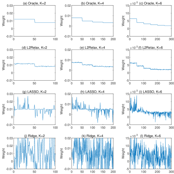
Figure 1: Illustration of the Estimated Weights in DGP 1

The six panels in Table 1 report the out-of-sample prediction accuracy by MSFE for all three DGPs with low and high SNRs, respectively. The first three columns show the settings of $T$, $N$ and $K$, and the following columns show the MSFEs of the labeled estimators. All estimators have stronger performance under a high SNR than that under a low SNR. The rankings of relative performance among the six estimators are similar across different DGPs despite that the additional factor loading noises enlarge the MSFEs of all estimators from DGP 3 relative to those from DGP 1.

Table 1: Results of Prediction Accuracy by MSFE

	$T$	$N$	$K$	Oracle	SA	$\ell_{2}$-relax0	Lasso	Ridge	PC			$\ell_{2}$-relax
									$q=5$	$q=10$	$q=20$	$\widehat{\boldsymbol{\Sigma}}_{s}$	$\widehat{\boldsymbol{\Sigma}}_{1}$	$\widehat{\boldsymbol{\Sigma}}_{2}$
Panel A: DGP 1 with Low SNR
	50	100	2	0.312	0.891	1.536	0.402	1.253	0.679	0.662	0.667	0.393	0.366	0.342
	100	200	4	0.175	3.707	0.922	0.289	1.054	1.209	1.454	1.438	0.268	0.274	0.256
	200	300	6	0.077	4.469	0.295	0.139	0.386	1.233	1.358	1.415	0.133	0.122	0.102
Panel B: DGP 1 with High SNR
	50	100	2	0.259	0.938	0.574	0.311	0.502	0.702	0.730	0.710	0.274	0.271	0.267
	100	200	4	0.132	2.915	0.254	0.166	0.258	1.017	1.206	1.266	0.147	0.146	0.141
	200	300	6	0.101	3.975	0.213	0.123	0.136	1.274	1.285	1.284	0.120	0.122	0.114
Panel C: DGP 2 with Low SNR
	50	100	2	0.292	1.032	1.251	0.401	1.235	0.787	0.800	0.763	0.383	0.390	0.366
	100	200	4	0.133	3.052	0.763	0.236	1.010	1.134	1.275	1.531	0.219	0.258	0.274
	200	300	6	0.066	3.699	0.411	0.131	0.412	1.109	1.050	1.173	0.173	0.144	0.124
Panel D: DGP 2 with High SNR
	50	100	2	0.262	0.993	0.401	0.323	0.488	0.702	0.747	0.751	0.280	0.279	0.271
	100	200	4	0.146	3.210	0.255	0.185	0.274	1.030	1.257	1.428	0.160	0.167	0.154
	200	300	6	0.106	4.524	0.135	0.126	0.139	1.343	1.601	1.639	0.126	0.122	0.114
Panel E: DGP 3 with Low SNR
	50	100	2	0.430	1.017	1.581	1.055	1.518	0.837	0.952	0.901	0.541	0.486	0.443
	100	200	4	0.287	3.718	1.116	0.710	1.394	1.821	1.775	2.002	0.384	0.415	0.357
	200	300	6	0.234	4.702	0.935	0.484	0.869	1.856	2.175	2.400	0.256	0.281	0.262
Panel F: DGP 3 with High SNR
	50	100	2	0.378	1.148	0.761	0.757	0.765	0.941	0.969	0.993	0.412	0.410	0.392
	100	200	4	0.279	3.191	0.482	0.393	0.482	1.518	1.665	1.812	0.301	0.285	0.285
	200	300	6	0.263	4.536	0.458	0.317	0.347	2.055	2.096	2.180	0.297	0.313	0.278

The infeasible grouping information helps the oracle estimator to prevail in all cases. Regardless which $\widehat{\boldsymbol{\Sigma}}$ estimator is employed, $\ell_{2}$-relaxation outperforms feasible competitors and its MSFE approaches that of the oracle estimator. The $\ell_{2}$-relaxation with $\widehat{\boldsymbol{\Sigma}}_{2}$ generally achieves the best performance among all feasible estimators. Lasso and Ridge are in general better than the PC estimator. Given the group structures in the DGP, SA in general lags far behind the other feasible estimators that learn the combination weights from the data. Notice that the MSFEs by Oracle, $\ell_{2}$-relax⁰, Lasso, Ridge, and the $\ell_{2}$-relaxation decrease as $T$ grows along with $N$. However, the results by SA and PC under all values of $q$ may diverge as $(T,N)$ increases.

Our results are not sensitive to different evaluation methods. Bergmeir et al. (2018) argue that the standard 5-fold CV is valid in purely autoregressive models with uncorrelated errors. Simulation results for DGP 2 by the conventional 5-fold CV are reported in Appendix B.3. In summary, we observe robust performance of $\ell_{2}$-relaxation superior to the other feasible estimators across the DGP designs, signal strength, and CV methods.

4.2 Portfolio Analysis

We extend Fan et al. (2012)’s design to a simulated Fama-French five-factor model. Besides the market factor, Fama and French (2015) identify four additional factors capturing the size, value, profitability, and investment patterns in average stock returns. Let $R_{i}$ be the excessive return of the $i$th stock. The five-factor model is similar to (3.4):

$$r_{it}=\boldsymbol{\lambda}_{i}^{\prime}\boldsymbol{\eta}_{t}+u_{it},$$ (4.2)

where $\boldsymbol{\lambda}_{i}=\{\lambda_{ij}\}_{j=1}^{5}$ is the vector of 5 factor loadings.

Table 2: Parameters for the Portfolio Simulation

Parameters for Factor Returns							Parameters for Factor Loadings (Size-BM)
$\mathbf{\mu}_{f}$	$\mathbf{cov}_{f}$						$\mathbf{\mu}_{\lambda}$	$\mathbf{cov}_{\lambda}$
0.644	20.388	4.175	1.324	-4.530	-1.351		1.009	0.013	0.000	0.006	0.002	-0.005
0.280	4.175	7.129	2.111	-1.646	0.378		0.617	0.001	0.165	-0.029	-0.028	-0.006
-0.091	1.324	2.111	8.346	0.990	2.869		0.175	0.007	-0.030	0.143	0.028	0.002
0.306	-4.530	-1.646	0.990	4.855	0.751		-0.040	0.002	-0.028	0.028	0.061	0.015
0.107	-1.351	0.378	2.869	0.752	3.431		0.005	-0.005	-0.006	0.002	0.015	0.058
Parameters for Factor Loadings (Size-INV)							Parameters for Factor Loadings (Size-OP)
$\mathbf{\mu}_{\lambda}$	$\mathbf{cov}_{\lambda}$						$\mathbf{\mu}_{\lambda}$	$\mathbf{cov}_{\lambda}$
1.053	0.015	0.002	-0.008	-0.011	-0.000		1.060	0.017	0.002	-0.008	-0.004	-0.009
0.621	0.002	0.156	0.012	-0.033	-0.026		0.630	0.002	0.175	0.011	0.041	0.000
0.128	-0.007	0.012	0.026	0.031	0.010		0.169	-0.008	0.011	0.055	0.054	-0.008
-0.079	-0.010	-0.032	0.031	0.086	0.020		-0.033	-0.004	0.041	0.054	0.233	0.021
-0.055	-0.000	-0.025	0.010	0.020	0.159		-0.139	-0.009	0.000	-0.009	0.021	0.041

We simulate the returns for $N=100$ assets and $T=240$ months. The factors and factor loadings are generated from the multivariate normal distributions $N(\mathbf{\mu}_{f},\mathbf{cov}_{f})$ and $N(\mathbf{\mu}_{\lambda},\mathbf{cov}_{\lambda})$, respectively. The values of the parameters $(\mathbf{\mu}_{b},\mathbf{cov}_{b},\mathbf{\mu}_{f},\mathbf{cov}_{f})$ are displayed in Table 2, which are calibrated to the 2001–2020 real market data of Fama and French 100 portfolios on the size and book-to-market (Size-BM), size and investment (Size-INV), and size and operating profitability (Size-OP). The idiosyncratic noises are generated from $N(\mathbf{0},\mathbf{cov}_{u})$, where $\mathbf{cov}_{u}$ is the sample VC matrix of the residuals from the OLS estimation of (4.2).

Instead of MFSE, we use the Sharpe ratio as the criterion for MVP. The $\ell_{2}$-relaxation estimator allows negative weights, which correspond to short positions of financial assets. For each repetition, the following rolling window estimation is considered with window length $L$. We avoid recursively training models for each month. Following a similar strategy in Gu et al. (2020), we train and roll forward once every year, as elaborated in Box 4.

Table 3: Sharpe Ratios of Estimated Portfolios

$L$	$N$	SA		GEC			$\ell_{2}$-relax
				$c=1$	$c=2$		$\widehat{\boldsymbol{\Sigma}}_{s}$	$\widehat{\boldsymbol{\Sigma}}_{1}$	$\widehat{\boldsymbol{\Sigma}}_{2}$
Panel A: Size-BM
60	100	0.131		0.171	0.234		0.378	0.382	0.363
120	100	0.128		0.175	0.255		0.463	0.478	0.470
Panel B: Size-INV
60	100	0.154		0.176	0.206		0.283	0.284	0.271
120	100	0.158		0.180	0.216		0.339	0.353	0.344
Panel C: Size-OP
60	100	0.170		0.213	0.270		0.404	0.409	0.389
120	100	0.168		0.214	0.283		0.515	0.528	0.516

We consider training data of lengths $L=60$ (5 years) and 120 (10 years). The $\ell_{2}$-relaxation estimator is compared with SA and the gross exposure constraints (GEC) methods (Fan et al., 2012):

$$\min_{\mathbf{w}\in\mathbb{R}^{N}}\,\frac{1}{2}\mathbf{w}^{\prime}\widehat{\boldsymbol{\Sigma}}\mathbf{w}\ \ \text{subject to \ }\mathbf{w}^{\prime}\boldsymbol{1}_{N}=1\mbox{ and }\|\mathbf{w}\|_{1}\leq c,$$

where the exposure constraint is set as $c=1$ (no short exposure) or $c=2$ (allowing 50% short exposure). Table 3 reports the Sharpe ratios averaged over 1000 replications. The three panels correspond to portfolios sorted by Size-BM, Size-INV, and Size-OP, respectively. SA performs poorly in terms of yielding the lowest Sharpe ratios in all cases. GEC with a short exposure of 50% is better than those without. For the case of $\ell_{2}$-relaxation, the three choices of $\widehat{\boldsymbol{\Sigma}}$ lead to similar Sharpe ratios, which all outperform GEC and SA.

5 Empirical Applications

In this section, we explore three empirical examples. In the first two applications, we assess the MSFE of a microeconomic study of forecasting box office and a macroeconomic exercise for the survey of professional forecasters (SPF). The last one is a financial application of MVP evaluated by the Sharpe ratio.

5.1 Box Office

The motion picture industry devotes enormous resources to marketing in order to influence consumer sentiment toward their products. These resources are intended to reduce the supply-demand friction on the market. On the supply side, movie making is an expensive business; on the demand side, however, the audience’s taste is notoriously fickle. Accurate prediction of box office is financially crucial for motion picture investors.

Based on the data of Hollywood movies released in North America between October 1, 2010 and June 30, 2012, Lehrer and Xie (2017) demonstrate the sound out-of-sample performance of the prediction model averaging (PMA). We revisit their dataset of 94 cross-sectional observations (movies), 28 non-constant explanatory variables and 95 candidate forecasters according to a multitude of model specifications. Guided by the intuition that the input variables capturing similar characteristics are “closer” to one another, Lehrer and Xie (2017) cluster input variables into six groups in their Appendix D.1:

$$\text{{Key variables}}: \mathtt{\ Constant,Animation,Family,Weeks,Screens,VOL:T-1/-3}$$

$$\text{{Twitter Volume}}: \mathtt{\ T-21/-27,T-14/-20,T-7/-13,T-4/-6}$$

$$\text{{Twitter Sentiment}}: \mathtt{\ T-21/-27,T-14/-20,T-7/-13,T-4/-6,T-1/-3}$$

$$\text{{Rating Related}}: \mathtt{\ PG,PG13,R,Budget}$$

$$\text{{Male Genre}}: \mathtt{\ Action,Adventure,Crime,Fantasy,Sci-Fi,Thriller}$$

$$\text{{Female Genre}}: \mathtt{\ Comedy,Drama,Mystery,Romance}$$

Since the 95 forecasters are generated based on these input variables, the potential group patterns may help $\ell_{2}$-relaxation achieve more accurate forecasts than other off-the-shelf machine learning shrinkage methods in this setting.

Following Lehrer and Xie (2017), we randomly rearrange the full sample with $n=94$ movies into a training set of the size $n_{\mathrm{tr}}$ and an evaluation set of the size $n_{\mathrm{ev}}=n-n_{\mathrm{tr}}$, which we experiment with $n_{\mathrm{ev}}=10,$ $20,$ $30$, and 40. We repeat this procedure for 1,000 times and evaluate the MSFE of PMA, $\ell_{2}$-relax⁰, the CSR (Elliott et al., 2013), the peLASSO (Diebold and Shin, 2019), Lasso, Ridge, and $\ell_{2}$-relaxation. We choose the number of subset regressors to be 10 and 15 for the CSR approach, denoted as CSR₁₀ and CSR₁₅, respectively. Since the total number of candidate models is too large to handle, we follow Genre et al. (2013) and randomly pick 10000 candidate models instead. For peLASSO, we follow Diebold and Shin (2019) and conduct a two-step estimation (first Lasso, then Ridge). Movies are viewed as independent observations and thus the tuning parameters are chosen by the conventional 5-fold CV. We conduct a grid search from 0 to 5 with increment 0.1.

Table 4: Relative MSFE of Movie Forecasting

$n_{\mathrm{ev}}$	PMA	$\ell_{2}$-relax0	CSR10	CSR15	peLasso	Lasso	Ridge	$\ell_{2}$-relax
								$\widehat{\boldsymbol{\Sigma}}_{s}$	$\widehat{\boldsymbol{\Sigma}}_{1}$	$\widehat{\boldsymbol{\Sigma}}_{2}$
10	1.000	5.075	2.564	3.475	4.518	1.085	1.073	0.933	0.903	0.863
20	1.000	3.088	2.461	3.697	3.837	1.167	1.167	0.924	0.864	0.836
30	1.000	3.122	1.660	2.689	3.004	1.161	1.236	0.914	0.825	0.722
40	1.000	3.112	1.107	1.891	1.736	1.028	1.169	0.904	0.851	0.692
Note: The MSFE of PMA is normalized as 1.

Since the magnitude of MSFEs varies on the evaluation sizes $n_{\mathrm{ev}}$, we report in Table 4 the mean risk relative to that of PMA for convenience of comparison. Entries smaller than 1 indicate better performance relative to that of PMA. While PMA is known to outperform Lasso and Ridge in Lehrer and Xie (2017), in this exercise it also outperforms $\ell_{2}$-relax⁰, CSR, and peLasso. Shrinkage toward the global equal weight $1/N$ or toward 0 is not favored in this experiment. $\ell_{2}$-relaxation, on the other hand, yields lower risk than PMA under any $\widehat{\boldsymbol{\Sigma}}$, and the edge generally increases with the value of $n_{\mathrm{ev}}$.

To demonstrate the potential grouping pattern in the data, we show the estimated weights of a typical replication on $n_{\mathrm{ev}}=10$ and $\tau=1$ in Figure 2. The pattern is similar for other values of $n_{\mathrm{ev}}$. The vertical axis of Figure 2 represents the estimated weights, and the horizontal axis shows all the 95 forecasters order by the weights from high to low. In addition, we divide the weights into five groups according to the following manually selected intervals: $(-\infty,-0.05)$, $(0.05,0)$, $(0,0.05)$, $(0.05,0.2)$, and $(0.2,+\infty)$. Circles and solid-lines represent the weights and group means, respectively, in Figure 2. The results demonstrate potential latent grouping pattern. Interesting, more than 40% of the individual models receive negative weights.

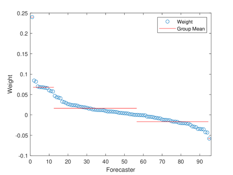
Figure 2: Estimated Weights by $\ell_{2}$-relaxation ($n_{\text{ev}}=10$ and $\tau=1$)

5.2 Inflation

Firms, consumers, as well as monetary policy authorities count on the outlook of inflation to make rational economic decisions. Besides model-based inflation forecasts published by government and research institutes, SPF reports experts’ perceptions about the price level movement in the future. A long-standing myth of forecast combination lies in the robustness of the simple average which extract the mean or median as a predictor in a simple linear regression, as documented by Ang et al. (2007). Recent research shows modern machine learning methods can assist by assigning data-driven weights to individual forecasters to gather disaggregate information; see, e.g., Diebold and Shin (2019).

The European Central Bank’s SPF inquires many professional institutions for their expectations of the euro-zone macroeconomic outlook. We revisit Genre et al. (2013)’s harmonized index of consumer prices (HICP) dataset, which covers 1999Q1–2018Q4. The experts were asked about their one-year- and two-year-ahead predictions. The raw data record 119 forecasters in total, but are highly unbalanced with plenty of missing values, mainly due to entry and exit in the long time span. We follow Genre et al. (2013) to obtain 30 qualified forecasters by first filtering out irregular respondents if he or she missed more than 50% of the observations, and then using a simple AR(1) regression to interpolate the missing values in the middle.

Table 5: Relative MSFE of HICP Forecasting

Horizon	SA	$\ell_{2}$-relax0	Lasso	Ridge	$\ell_{2}$-relax
					$\widehat{\boldsymbol{\Sigma}}_{s}$	$\widehat{\boldsymbol{\Sigma}}_{1}$	$\widehat{\boldsymbol{\Sigma}}_{2}$
One-year-ahead	1.000	2.029	0.844	0.869	0.908	0.777	0.824
Two-year-ahead	1.000	1.947	0.750	0.910	0.684	0.728	0.602
Note: The MSFE of SA is normalized as 1.

Our benchmark is the simple average (SA) on all 30 forecasters. We compare the forecast errors of SA, $\ell_{2}$-relax⁰, Lasso, Ridge, and $\ell_{2}$-relaxation. We use a rolling window of 40 quarters for estimation. The tuning parameters are selected by the OOS approach described in Box 2 with grid search from 0 to 5 with increment 0.01. The results of relative risks are presented in Table 5, with the MSFEs of SA standardized as 1. $\ell_{2}$-relax⁰ performs worse than SA. Lasso and Ridge yield roughly 15% improvement relative to SA. $\ell_{2}$-relaxation exhibits robust performance under all choices of $\widehat{\boldsymbol{\Sigma}}$.

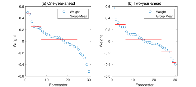
Figure 3: $\ell_{2}$-relaxation’s Estimated Weights under the Two Horizons

Since we do not directly observe the underlying factors based upon which the forecasters make decisions, we illustrate in Figure 3 the estimated weights associated with the 30 forecasters of a typical roll from 1999Q1 to 2008Q4 and $\tau=0.02$. Sub-figures (a) and (b) are associated with results of one-year-ahead and two-year-ahead forecasting, respectively. The horizontal axis shows the forecasters and the vertical axis represents the estimated weights. The weights can be roughly categorized into five groups according to the following manually selected intervals: $(-\infty,-0.3)$, $(-0.3,-0.1)$, $(-0.1,0.2)$, $(0.2,0.4)$, and $(0.4,+\infty)$. In both sub-figures, the spread of the weights deviates the equal-weight SA strategy. In sub-figure (b) the weights are more concentrated around 0 than sub-figure (a), reflecting the challenges to forecast over a longer horizon.

5.3 Fama and French 100 Portfolios

Here we mimic the simulation design in Section 4.2 but feed the algorithms with the real 2001–2020 Fama and French 100 monthly portfolios on Size-BM, Size-INV, and Size-OP. The empirical results are presented in Table 6.

Table 6: Sharp Ratio based on 100 Fama-French Portfolios

$L$	$N$	SA		GEC			$\ell_{2}$-relax
				$c=1$	$c=2$		$\widehat{\boldsymbol{\Sigma}}_{s}$	$\widehat{\boldsymbol{\Sigma}}_{1}$	$\widehat{\boldsymbol{\Sigma}}_{2}$
Panel A: Size-BM
60	100	0.182		0.210	0.257		0.277	0.264	0.265
120	100	0.249		0.362	0.428		0.441	0.428	0.445
Panel B: Size-INV
60	100	0.191		0.296	0.255		0.192	0.215	0.232
120	100	0.252		0.335	0.340		0.414	0.426	0.407
Panel C: Size-OP
60	100	0.222		0.293	0.383		0.342	0.314	0.335
120	100	0.287		0.431	0.513		0.472	0.548	0.541

The benchmark SA suggested by DeMiguel et al. (2009) delivers higher Sharpe ratios under the longer rolling window, indicating substantial noise in the simple aggregation over the cross section when $L$ is small. The performance of SA is eclipsed by GEC and $\ell_{2}$-relaxation in all cases. GEC without short exposure ($c=1$) wins the Size-INV with $L=60$, and that with 50% short exposure ($c=2$) wins the Size-OP with $L=60$. In four out of six cases, nevertheless, $\ell_{2}$-relaxation delivers the highest Sharpe ratios.

Sub-figure 4.1: Size-BM

(a)

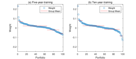
Sub-figure 4.2: Size-INV

(b)

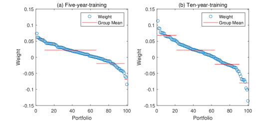
Sub-figure 4.3: Size-OP

(c)

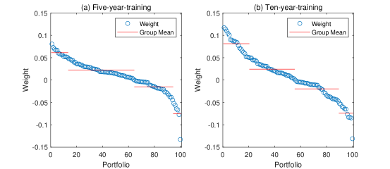
Figure 4: Estimated Weights by $\ell_{2}$-relaxation

To better understand the behavior of $\ell_{2}$-relaxation, we plot in Figure 4 its estimated weights of a typical estimation window with $L=60$ and 120, and the value of tuning parameter set to $\tau=1$. We assign the 100 portfolios into 5 groups in each case and plot the group means by the red horizontal lines. The weights are manually categorized into five intervals: $(-\infty,-0.05)$, $(-0.05,0)$, $(0,0.05)$, $(0.05,0.15)$, and $(0.15,+\infty)$. The distribution of the weights are similar across $L$ in the sub-figure for the Size-BM sorted portfolios. Under the Size-INV sorting, however, the weights for $L=60$ are less spread and many are close to zero, and the weights under the Size-OP portfolios share similar patterns. This phenomenon helps to explain the high Sharpe ratio of GEC under $L=60$: intuitively, its $\ell_{1}$-norm restriction $\|\mathbf{w}\|_{1}\leq c$ would shrink all weights toward zero and moreover push many small weights to be exactly zero.

Acknowledging that the theoretical setup of parsimonious factors and group structure is an approximation of the real financial world at best, in future studies we are interested in investigating an enhanced $\ell_{2}$-relaxation with the exposure constraint $\|\mathbf{w}\|_{1}\leq c$.

6 Conclusion

This paper presents a new machine learning algorithm, namely, $\ell_{2}$-relaxation. When the forecast error VC or the portfolio VC can be approximated by a block equicorrelation structure, we establish its consistency and asymptotic optimality in the high dimensional context. Simulations and real data applications demonstrate excellent performance of the $\ell_{2}$-relaxation method.

Our work raises several interesting issues for further research. First, we have not studied the optimal choice of the tuning parameter $\tau$ or provided a formal justification for the use of the cross-validated $\tau.$ Recently, Wu and Wang (2020) have reviewed the literature of tuning parameter selection for high dimensional regressions and discussed various strategies to choose the tuning parameter to achieve either prediction accuracy or support recovery such as the $L$-fold cross-validation, $m$-out-of-$n$ bootstrap and extended Bayesian information criterion (BIC). Chetverikov et al. (2021) have studied the theoretical properties of Lasso based on cross-validated choice of the tuning parameter. It will be interesting to study whether we can draw support from these papers to provide theoretical guidance concerning the choice of $\tau$ in our context.

Second, additional restrictions can be imposed to accompany the $\ell_{2}$-relaxation problem. For example, if sparsity is desirable, we may consider adding the exposure constraint $\left\|\mathbf{w}\right\|_{1}\leq c$ for some tuning parameter $c$, which echoes the idea of mixed $\ell_{1}$- and $\ell_{2}$-penalty of the elastic net method by Zou and Hastie (2005). Another example is to incorporate the constraints $w_{i}\geq 0$ for all $i$ if non-negative weights are desirable (Jagannathan and Ma, 2003). Third, our $\ell_{2}$-relaxation is motivated from the MSFE loss function, it is possible to consider other forms of relaxation if the other forms of loss functions (e.g., MAFE) are under investigation. Last but not least, the $\ell_{2}$-relaxation theory in this paper requires the dominant component $\mathbf{\hat{\Sigma}}^{\ast}$ of the VC matrix to have a latent group structure. It is desirable to extend the theory to the case where $\mathbf{\hat{\Sigma}}^{\ast}$ has only a low-rank structure instead of a latent group structure. We shall explore some of these topics in future works.

This online appendix is composed of two sections. Appendix A contains the proofs of the theoretical results in the paper. Appendix B contains some additional results on the simulation and empirical exercises.

Additional Notation. The notations in the appendix are consistent with those in the main text. Here we introduce a few additional expressions. For a generic $n\times m$ matrix $\mathbf{B}$, we denote $\mathbf{B}_{i\cdot}$ as the $i$-th row ($1\times m$ vector), and define the spectral norm as $\left\|\mathbf{B}\right\|_{\mathrm{sp}}:=\phi_{\max}^{1/2}\left(\mathbf{B}^{\prime}\mathbf{B}\right)$. “w.p.a.1” is short for “with probability approaching one” in asymptotic statements.

Appendix A Technical Appendix

A.1 Optimization Formulation

While the original paper of Bates and Granger (1969) consider unbiased forecasts in that $E\left[y_{t+1}-f_{it}\right]=0$ for all $i$, Granger and Ramanathan (1984) generalize it to accommodate biased forecasts. We start with the latter. Besides the $N\times 1$ weight vector $\mathbf{w}$, we seek an additional intercept $\mu$, which is an unknown location parameter, to correct the bias of the combined forecasts. The optimization problem can be written as

$$\min_{\left(\mu,\mathbf{w}\right)\in\mathbb{R}^{N+1}}\ \frac{1}{2T}\sum_{t=1}^{T}\left(y_{t+1}-\mu-\mathbf{w}^{\prime}\mathbf{f}_{t}\right)^{2}\ \text{subject to\ }\boldsymbol{1}_{N}^{\prime}\mathbf{w}=1.$$

Its Lagrangian is

$$L\left(\mu,\mathbf{w},\gamma\right) =\frac{1}{2T}\sum_{t=1}^{T}\left(y_{t+1}-\mu-\mathbf{w}^{\prime}\mathbf{f}_{t}\right)^{2}+\gamma\left(\boldsymbol{1}_{N}^{\prime}\mathbf{w}-1\right)$$

$$=\frac{1}{2T}\sum_{t=1}^{T}\left(\mathbf{w}^{\prime}\left[\left(y_{t+1}-\mu\right)\boldsymbol{1}_{N}-\mathbf{f}_{t}\right]\right)^{2}+\gamma\left(\boldsymbol{1}_{N}^{\prime}\mathbf{w}-1\right)$$

$$=\frac{1}{2T}\mathbf{w}^{\prime}\left[\sum_{t=1}^{T}\left(\mathbf{e}_{t}-\mu\boldsymbol{1}_{N}\right)\left(\mathbf{e}_{t}-\mu\boldsymbol{1}_{N}\right)^{\prime}\right]\mathbf{w}+\gamma\left(\boldsymbol{1}_{N}^{\prime}\mathbf{w}-1\right),$$

where $\gamma$ is the Lagrangian multiplier. The above formulation includes Bates and Granger (1969)’s problem as a special case when $\mu=0$.

When $\mu$ is unconstrained, given any $\mathbf{w}$ its minimizer is $\widehat{\mu}=\widehat{\mu}\left(\mathbf{w}\right)=\mathbf{w}^{\prime-1}\sum_{t=1}^{T}\mathbf{e}_{t}=\mathbf{w}^{\prime}\bar{\mathbf{e}}$. Substituting $\widehat{\mu}$ back to the Lagrangian to profile out $\mu$ yields

$$\widehat{L}\left(\mathbf{w},\gamma\right) :=L\left(\widehat{\mu}\left(\mathbf{w}\right),\mathbf{w},\gamma\right)$$

$$=\frac{1}{2}\mathbf{w}^{\prime}\left[\frac{1}{T}\sum_{t=1}^{T}\left(\mathbf{e}_{t}-\bar{\mathbf{e}}\right)\left(\mathbf{e}_{t}-\bar{\mathbf{e}}\right)^{\prime}\right]\mathbf{w}+\gamma\left(\boldsymbol{1}_{N}^{\prime}\mathbf{w}-1\right)$$

$$=\frac{1}{2}\mathbf{w}^{\prime}\widehat{\boldsymbol{\Sigma}}\mathbf{w}+\gamma\left(\boldsymbol{1}_{N}^{\prime}\mathbf{w}-1\right),$$ (A.1)

which is exactly the Lagrangian of the problem in (1.1).

A.2 Finite Sample Numerical Properties

The primal problem in (2.5) induces the dual problem as stated in the following lemma. (A.2) below is a constrained $\ell_{1}$-penalized optimization where the criterion function is the summation of a quadratic form of $\boldsymbol{\alpha}$, a linear combination of $\boldsymbol{\alpha}$, and the $\ell_{1}$-norm of $\boldsymbol{\alpha}$, while the constraint is linear in $\boldsymbol{\alpha}$. The dual problem is instrumental in our theoretical analyses due to its similarity to Lasso (Tibshirani, 1996).

Lemma S2.

The dual problem of (2.5) is

$$\min_{\boldsymbol{\alpha}\in\mathbb{R}^{N}}\left\{\frac{1}{2}\boldsymbol{\alpha}^{\prime}\widehat{\mathbf{A}}^{\prime}\widehat{\mathbf{A}}\boldsymbol{\alpha}+\frac{1}{N}\boldsymbol{1}_{N}^{\prime}\widehat{\boldsymbol{\Sigma}}\boldsymbol{\alpha}+\tau\left\|\boldsymbol{\alpha}\right\|_{1}-\frac{1}{2N}\right\}\text{\ \ subject to \ }\boldsymbol{1}_{N}^{\prime}\boldsymbol{\alpha}=0,$$ (A.2)

where $\widehat{\mathbf{A}}=\left(\mathbf{\mathbf{I}}_{N}-N^{-1}\boldsymbol{1}_{N}\boldsymbol{1}_{N}^{\prime}\right)\widehat{\boldsymbol{\Sigma}}$ is the columnwise demeaned version of $\widehat{\boldsymbol{\Sigma}}$. Denote $\widehat{\boldsymbol{\alpha}}=\widehat{\boldsymbol{\alpha}}_{\tau}$ as a solution to the dual problem in (A.2), and it is connected with the solution to the primal problem in (2.5) via

$$\widehat{\mathbf{w}}=\widehat{\mathbf{A}}\widehat{\boldsymbol{\alpha}}+\frac{\boldsymbol{1}_{N}}{N}.$$ (A.3)

Proof of Lemma S2. First, we can rewrite the minimization problem in (2.5) in terms of linear constraints:

$$\min_{\left(\mathbf{w},\gamma\right)\in\mathbb{R}^{N+1}}\frac{1}{2}\left\|\mathbf{w}\right\|_{2}^{2}$$

$$\text{s.t. }\mathbf{w}^{\prime}\boldsymbol{1}_{N}-1=0,\ \begin{pmatrix}\widehat{\boldsymbol{\Sigma}}&\boldsymbol{1}_{N}\end{pmatrix}\begin{pmatrix}\mathbf{w}\\ \gamma\end{pmatrix}\leq\tau\boldsymbol{1}_{N},\ \text{and }-\begin{pmatrix}\widehat{\boldsymbol{\Sigma}}&\boldsymbol{1}_{N}\end{pmatrix}\begin{pmatrix}\mathbf{w}\\ \gamma\end{pmatrix}\leq\tau\boldsymbol{1}_{N}$$ (A.4)

where “$\leq$” holds elementwise hereafter. Define the Lagrangian function as

$$\mathcal{L}\left(\mathbf{w},\gamma;\boldsymbol{\alpha}_{1},\boldsymbol{\alpha}_{2},\alpha_{3}\right) = \frac{1}{2}\mathbf{w}^{\prime}\mathbf{w}+\boldsymbol{\alpha}_{1}^{\prime}\left(\begin{pmatrix}\widehat{\boldsymbol{\Sigma}}&\boldsymbol{1}_{N}\end{pmatrix}\begin{pmatrix}\mathbf{w}\\ \gamma\end{pmatrix}-\tau\boldsymbol{1}_{N}\right)$$ (A.5)

$$-\boldsymbol{\alpha}_{2}^{\prime}\left(\begin{pmatrix}\widehat{\boldsymbol{\Sigma}}&\boldsymbol{1}_{N}\end{pmatrix}\begin{pmatrix}\mathbf{w}\\ \gamma\end{pmatrix}+\tau\boldsymbol{1}_{N}\right)+\alpha_{3}\left(\mathbf{w}^{\prime}\boldsymbol{1}_{N}-1\right)$$

and the associated Lagrangian dual function as $g\left(\boldsymbol{\alpha}_{1},\boldsymbol{\alpha}_{2},\alpha_{3}\right)=\inf_{\mathbf{w},\gamma}\mathcal{L}\left(\mathbf{w},\gamma;\boldsymbol{\alpha}_{1},\boldsymbol{\alpha}_{2},\alpha_{3}\right),$ where $\boldsymbol{\alpha}_{1}\geq 0$, $\boldsymbol{\alpha}_{2}\geq 0$, and $\alpha_{3}$ are the Lagrangian multipliers for the three constraints in (A.4), respectively.

Let $\varphi\left(\mathbf{w,}\gamma\right)=\frac{1}{2}\left\|\mathbf{w}\right\|_{2}^{2}$, the objective function in (A.4). Define its conjugate function as

$$\varphi^{\ast}\left(\mathbf{a,}b\right)=\sup_{\mathbf{w},\gamma}\left\{\mathbf{a}^{\prime}\mathbf{w}+b\gamma-\frac{1}{2}\left\|\mathbf{w}\right\|_{2}^{2}\right\}=\left\{\begin{array}[]{ll}\frac{1}{2}\left\|\mathbf{a}\right\|_{2}^{2}\text{ }&\text{if }b=0\\ \infty&\text{otherwise}\end{array}.\right.$$

The linear constraints indicate an explicit dual function (See Boyd and Vandenberghe (2004, p.221)):

$$g\left(\boldsymbol{\alpha}_{1},\boldsymbol{\alpha}_{2},\alpha_{3}\right)$$

$$= -\tau\boldsymbol{1}_{N}^{\prime}\left(\boldsymbol{\alpha}_{1}+\boldsymbol{\alpha}_{2}\right)-\alpha_{3}-\varphi^{\ast}\left(\widehat{\boldsymbol{\Sigma}}\left(\boldsymbol{\alpha}_{2}-\boldsymbol{\alpha}_{1}\right)-\alpha_{3}\boldsymbol{1}_{N},\text{ }\boldsymbol{1}_{N}^{\prime}\left(\boldsymbol{\alpha}_{2}-\boldsymbol{\alpha}_{1}\right)\right)$$

$$= \left\{\begin{array}[]{ll}-\tau\boldsymbol{1}_{N}^{\prime}\left(\boldsymbol{\alpha}_{1}+\boldsymbol{\alpha}_{2}\right)-\alpha_{3}-\frac{1}{2}\left\|\widehat{\boldsymbol{\Sigma}}\left(\boldsymbol{\alpha}_{2}-\boldsymbol{\alpha}_{1}\right)-\alpha_{3}\boldsymbol{1}_{N}\right\|_{2}^{2},\text{ }&\text{if }\boldsymbol{1}_{N}^{\prime}\left(\boldsymbol{\alpha}_{2}-\boldsymbol{\alpha}_{1}\right)=0\\ \infty,&\text{otherwise}\end{array}.\right.$$

Let $\boldsymbol{\alpha}=\boldsymbol{\alpha}_{2}-\boldsymbol{\alpha}_{1}$. When $\tau>0$, the two inequalities $\widehat{\boldsymbol{\Sigma}}_{i\cdot}\mathbf{w}+\gamma\leq\tau$ and $-\widehat{\boldsymbol{\Sigma}}_{i\cdot}\mathbf{w}-\gamma\leq\tau$ cannot be binding simultaneously. The associated Lagrangian multipliers $\alpha_{1i}$ and $\alpha_{2i}$ must satisfy $\alpha_{1i}\cdot\alpha_{2i}=0$ for all $i\in\left[N\right]$. This implies that $\left\|\boldsymbol{\alpha}\right\|_{1}=\boldsymbol{1}_{N}^{\prime}\boldsymbol{\alpha}_{1}+\boldsymbol{1}_{N}^{\prime}\boldsymbol{\alpha}_{2}$ so that the dual problem can be simplified as

$$\max_{\boldsymbol{\alpha},\alpha_{3}}\left\{-\frac{1}{2}\left\|\widehat{\boldsymbol{\Sigma}}\boldsymbol{\alpha}-\alpha_{3}\boldsymbol{1}_{N}\right\|_{2}^{2}-\alpha_{3}-\tau\left\|\boldsymbol{\alpha}\right\|_{1}\right\}\ \text{ s.t. }\boldsymbol{1}_{N}^{\prime}\boldsymbol{\alpha}=0.$$ (A.7)

Taking the partial derivative of the above criterion function with respect to $\alpha_{3}$ yields

$$(\widehat{\boldsymbol{\Sigma}}\boldsymbol{\alpha}-\alpha_{3}\boldsymbol{1}_{N})^{\prime}\boldsymbol{1}_{N}-1=0,$$

or equivalently, $\alpha_{3}=\frac{1}{N}(\boldsymbol{1}_{N}^{\prime}\widehat{\boldsymbol{\Sigma}}\boldsymbol{\alpha}-1).$ Then

$$\left\|\widehat{\boldsymbol{\Sigma}}\boldsymbol{\alpha}-\alpha_{3}\boldsymbol{1}_{N}\right\|_{2}^{2}=\left\|\widehat{\mathbf{A}}\boldsymbol{\alpha}+\frac{\boldsymbol{1}_{N}}{N}\right\|_{2}^{2}=\boldsymbol{\alpha}^{\prime}\widehat{\mathbf{A}}^{\prime}\widehat{\mathbf{A}}\boldsymbol{\alpha}+\frac{1}{N}$$

where $\widehat{\mathbf{A}}=\left(\mathbf{\mathbf{I}}_{N}-N^{-1}\boldsymbol{1}_{N}\boldsymbol{1}_{N}^{\prime}\right)\widehat{\boldsymbol{\Sigma}}$. We conclude that the dual problem in (A.7) is equivalent to

$$\min_{\boldsymbol{\alpha}\in\mathbb{R}^{N}}\left\{\frac{1}{2}\boldsymbol{\alpha}^{\prime}\widehat{\mathbf{A}}^{\prime}\widehat{\mathbf{A}}\boldsymbol{\alpha}+\frac{1}{N}\boldsymbol{1}_{N}^{\prime}\widehat{\boldsymbol{\Sigma}}\boldsymbol{\alpha}+\tau\left\|\boldsymbol{\alpha}\right\|_{1}-\frac{1}{2N}\right\}\text{ subject to }\boldsymbol{1}_{N}^{\prime}\boldsymbol{\alpha}=0,$$ (A.8)

where we keep the constant $-\frac{1}{2N}$ which is irrelevant to the optimization.

When $\widehat{\boldsymbol{\alpha}}=\widehat{\boldsymbol{\alpha}}_{2}-\widehat{\boldsymbol{\alpha}}_{1}$ is the solution to (A.8), the solution of $\alpha_{3}$ in (A.7) is $\widehat{\alpha}_{3}=\frac{1}{N}(\boldsymbol{1}_{N}^{\prime}\widehat{\boldsymbol{\Sigma}}\widehat{\boldsymbol{\alpha}}-1).$ The first order condition of (A.5) with respect to $\mathbf{w}$ evaluated at the solution gives

$$\boldsymbol{0}_{N}=\widehat{\mathbf{w}}+\widehat{\boldsymbol{\Sigma}}(\widehat{\boldsymbol{\alpha}}_{1}-\widehat{\boldsymbol{\alpha}}_{2})+\widehat{\alpha}_{3}\mathbf{1}_{N}=\widehat{\mathbf{w}}-\widehat{\boldsymbol{\Sigma}}\widehat{\boldsymbol{\alpha}}+\frac{1}{N}(\boldsymbol{1}_{N}^{\prime}\widehat{\boldsymbol{\Sigma}}\widehat{\boldsymbol{\alpha}}-1)\mathbf{1}_{N}=\widehat{\mathbf{w}}-\widehat{\boldsymbol{\Sigma}}\widehat{\boldsymbol{\alpha}}-\frac{1}{N}\mathbf{1}_{N}.$$

as $\boldsymbol{1}^{\prime}_{N}\widehat{\boldsymbol{\alpha}}=0$. The result in (A.3) follows. ${\ \blacksquare}$

Remark 6.

Since $\mathrm{rank}(\widehat{\mathbf{A}})\leq\mathrm{rank}(\mathbf{\mathbf{I}}_{N}-N^{-1}\boldsymbol{1}_{N}\boldsymbol{1}_{N}^{\prime})=N-1$, the singularity of $\widehat{\mathbf{A}}$ may induce multiple solutions to the dual problem in (A.2). Despite this, the uniqueness of $\widehat{\mathbf{w}}$ as a solution to the primal problem in (2.5) implies $\widehat{\mathbf{A}}\widehat{\boldsymbol{\alpha}}^{\left(1\right)}=\widehat{\mathbf{A}}\widehat{\boldsymbol{\alpha}}^{\left(2\right)}$ for any $\widehat{\boldsymbol{\alpha}}^{\left(1\right)}$ and $\widehat{\boldsymbol{\alpha}}^{\left(2\right)}$ that solve (A.2). It is sufficient to find any solution to the dual problem to recover the same $\widehat{\mathbf{w}}$ in the primal.

Next, we prove Lemma 1 that the oracle primal problem induces a within-group equal weight solution.

Proof of Lemma 1. The restriction of (3.7) can be written as

$$\begin{pmatrix}\widehat{\boldsymbol{\Sigma}}^{\ast}&\boldsymbol{1}_{N}\\ \boldsymbol{1}_{N}^{\prime}&0\end{pmatrix}\begin{pmatrix}\mathbf{w}\\ \gamma\end{pmatrix}=\begin{pmatrix}\boldsymbol{0}_{N}\\ 1\end{pmatrix}.$$

Since the rank of $\widehat{\boldsymbol{\Sigma}}^{\ast}$ is $K$ and there are an infinite number of solutions of $\left(\mathbf{w},\gamma\right)$ to the above system of $N+1$ equations. Since the $i$th equation and the $j$th equation are exactly the same if $i$ and $j$ are the in the same group, the $\left(N+1\right)$-equation system can be reduced to a system of $K+1$ equations:

$$\begin{pmatrix}\widehat{\boldsymbol{\Sigma}}^{\mathrm{co}}&\boldsymbol{1}_{K}\\ \boldsymbol{1}_{K}^{\prime}&0\end{pmatrix}\left(\sum_{i\in\mathcal{G}_{1}}w_{i},\ldots,\sum_{i\in\mathcal{G}_{K}}w_{i},\gamma\right)^{\prime}=\begin{pmatrix}\boldsymbol{0}_{K}\\ 1\end{pmatrix}.$$

Due to the $\ell_{2}$ criterion, the within-group weight takes equal value. Define $r_{k}:=N_{k}/N$ as the fraction of the $k$-th group members on the cross section. Let $\mathbf{r}=\left(r_{k}\right)_{k\in[K]}$ and $\mathbf{r}^{-1}=\left(r_{k}^{-1}\right)_{k\in[K]}$. Let “$\circ$” denote the Hadamard product. As $\widehat{\boldsymbol{\Sigma}}^{\mathrm{co}}$ is of full rank, the solution to the above $\left(K+1\right)$-equation system is unique:

$$\mathbf{b}_{0}^{\ast}\circ\mathbf{r}=\left(\sum_{i\in\mathcal{G}_{1}}w_{i}^{\ast},\ldots,\sum_{i\in\mathcal{G}_{K}}w_{i}^{\ast}\right)^{\prime}=\frac{(\widehat{\boldsymbol{\Sigma}}^{\mathrm{co}})^{-1}\boldsymbol{1}_{K}}{\boldsymbol{1}_{K}^{\prime}(\widehat{\boldsymbol{\Sigma}}^{\mathrm{co}})^{-1}\boldsymbol{1}_{K}}.$$

The explicit solution

$$\mathbf{b}_{0}^{\ast}:=\left(b_{0k}^{\ast}\right)_{k\in[K]}=\mathbf{r}^{-1}\circ\frac{(\widehat{\boldsymbol{\Sigma}}^{\mathrm{co}})^{-1}\boldsymbol{1}_{K}}{\boldsymbol{1}_{K}^{\prime}(\widehat{\boldsymbol{\Sigma}}^{\mathrm{co}})^{-1}\boldsymbol{1}_{K}}$$ (A.9)

follows immediately. ${\ \blacksquare}$

Remark 7.

In the portfolio analysis (2.3) the corresponding oracle problem can be written as

$$\min_{\left(\mathbf{w},\gamma\right)\in\mathbb{R}^{N+1}}\frac{1}{2}\left\|\mathbf{w}\right\|_{2}^{2}\text{\ \ subject to \ }\boldsymbol{1}_{N}^{\prime}\mathbf{w}=1,\ \ \bar{\mathbf{r}}^{\prime}\mathbf{w}\geq r^{*},\text{ and }\widehat{\boldsymbol{\Sigma}}^{\ast}\mathbf{w}+\gamma\mathbf{1}_{N}=0.$$ (A.10)

The solution to the above problem will be affected by the patterns in both $\widehat{\boldsymbol{\Sigma}}^{\ast}$ and $\bar{\mathbf{r}}$. Unlikely the within-group equal weight solution in Lemma 1, if the elements in $\bar{\mathbf{r}}$ take distinctive values, the corresponding $\widehat{\mathbf{w}}^{\ast}$ will not share within-group equal weights in view of the group membership defined solely by $\widehat{\boldsymbol{\Sigma}}^{\ast}$. This observation motivates us to focus on MVP, instead of the one with the mean return constraint.

To proceed, we define some notations about group patterns. We call a vector of similar sign if no pair of its elements takes opposite signs. Formally, an $n$-vector $\mathbf{b}$ is of similar sign if $\mathbf{b}\in\mathbb{S}^{n}:=\left\{\mathbf{b}\in\mathbb{R}^{n}:b_{i}b_{j}\geq 0\ \text{ for all }i,j\in\left[N\right]\right\}$. Let $\mathcal{G}_{1},\ldots,\mathcal{G}_{K}$ be a partition of $\left[N\right]$, and denote $N_{k}=\left|\mathcal{G}_{k}\right|$. We call a generic $N$-vector $\mathbf{b}$ of similar sign within all groups if $\mathbf{b}\in\mathbb{S}^{\mathrm{all}}:=\left\{\mathbf{b}\in\mathbb{R}^{N}:\mathbf{b}_{\mathcal{G}_{k}}\in\mathbb{S}^{N_{k}}\text{ for all }k\in[K]\right\}$, and define $\tilde{\mathbb{S}}^{\mathrm{all}}:=\left\{\mathbf{b}\in\mathbb{S}^{\mathrm{all}}:\boldsymbol{1}_{N}^{\prime}\mathbf{b}=0\right\}$ with a further restriction that the elements in $\mathbf{b}$ add up to 0.

Let $\phi_{e}:=\|\widehat{\boldsymbol{\Sigma}}^{e}\|_{c2}$ be a measurement of the noise level or contamination level of $\widehat{\boldsymbol{\Sigma}}^{\ast}$ in the model. Theorem 3 below characterizes the numerical properties of the sample estimator, where the condition $\tau>\phi_{e}\left\|\mathbf{b}_{0}^{\ast}\right\|_{\infty}/\sqrt{N}$ will be satisfied w.p.a.1 in the asymptotic analysis.

Theorem 3.

Suppose that $\tau>\phi_{e}\left\|\mathbf{b}_{0}^{\ast}\right\|_{\infty}/\sqrt{N}$. Then

1. $\left\|\widehat{\mathbf{w}}\right\|_{2}\leq\left\|\mathbf{w}^{*}\right\|_{2}\leq\left\|\mathbf{b}_{0}^{*}\right\|_{\infty}/\sqrt{N}$;

2. $\widehat{\boldsymbol{\alpha}}\in\mathbb{S}^{\mathrm{all}}$.

Proof of Theorem 3. Part (a). Substituting $\left(\mathbf{w}^{\ast},\gamma^{\ast}\right)$ into the constraint in (2.5), we obtain

$$\left\|\widehat{\boldsymbol{\Sigma}}\mathbf{w}^{\ast}+\gamma^{\ast}\boldsymbol{1}_{N}\right\|_{\infty} =\|\widehat{\boldsymbol{\Sigma}}^{\ast}\mathbf{w}^{\ast}+\widehat{\boldsymbol{\Sigma}}^{e}\mathbf{w}^{\ast}+\gamma^{\ast}\boldsymbol{1}_{N}\|_{\infty}=\|\widehat{\boldsymbol{\Sigma}}^{e}\mathbf{w}^{\ast}\|_{\infty}$$

$$=\max_{i}\|\widehat{\boldsymbol{\Sigma}}_{i\cdot}^{e}\mathbf{w}^{\ast}\|_{\infty}\leq\|\widehat{\boldsymbol{\Sigma}}^{e}\|_{c2}\|\mathbf{w}^{\ast}\|_{2}\leq\phi_{e}\|\mathbf{b}_{0}^{\ast}\|_{\infty}/\sqrt{N}.$$ (A.11)

where the second equality follows by the KKT condition $\widehat{\boldsymbol{\Sigma}}^{\ast}\mathbf{w}^{\ast}+\gamma^{\ast}\boldsymbol{1}_{N}=0$. The presumption $\phi_{e}\left\|\mathbf{b}_{0}^{\ast}\right\|_{\infty}/\sqrt{N}<\tau$ in the statement makes sure that $\|\widehat{\boldsymbol{\Sigma}}\mathbf{w}^{\ast}+\gamma^{\ast}\boldsymbol{1}_{N}\|_{\infty}<\tau$ holds with strict inequality. This strict inequality means that $\left(\mathbf{w}^{\ast},\gamma^{\ast}\right)$ lies in the interior of the feasible set of (2.5). Because $\widehat{\mathbf{w}}$ is the minimizer of the problem in (2.5), its $\ell_{2}$-norm is no greater than any other feasible solution. Thus $\left\|\widehat{\mathbf{w}}\right\|_{2}\leq\left\|\mathbf{w}^{\ast}\right\|_{2}$ and furthermore $\left\|\mathbf{w}^{\ast}\right\|_{2}$ is bounded by $\left\|\mathbf{b}_{0}^{\ast}\right\|_{\infty}/\sqrt{N}$ by Lemma 1.

Part (b). The Lagrangian of (A.2) can be written as

$$\mathcal{L}\left(\boldsymbol{\alpha},\gamma\right)=\frac{1}{2}\boldsymbol{\alpha}^{\prime}\widehat{\mathbf{A}}^{\prime}\widehat{\mathbf{A}}\boldsymbol{\alpha}+\frac{1}{N}\boldsymbol{1}_{N}^{\prime}\widehat{\boldsymbol{\Sigma}}\boldsymbol{\alpha}+\tau\left\|\boldsymbol{\alpha}\right\|_{1}+\gamma\boldsymbol{1}_{N}^{\prime}\boldsymbol{\alpha-}\frac{1}{2N},$$

where $\gamma$ is the Lagrangian multiplier for the constraint $\boldsymbol{1}_{N}^{\prime}\boldsymbol{\alpha}=0$. Consider the subgradient of $\mathcal{L}\left(\widehat{\boldsymbol{\alpha}},\widehat{\gamma}\right)$ with respect to $\alpha_{i}$ for any $i\in[N]$, where $\left(\widehat{\boldsymbol{\alpha}},\widehat{\gamma}\right)$ is the optimizer. Noting that $\widehat{\mathbf{A}}^{\prime}\widehat{\mathbf{A}}=\widehat{\mathbf{A}}^{\prime}\widehat{\boldsymbol{\Sigma}}$ due to the fact that $\mathbf{\mathbf{I}}_{N}-N^{-1}\boldsymbol{1}_{N}\boldsymbol{1}_{N}^{\prime}$ is a projection matrix, the KKT conditions imply that

$$\left|\widehat{\boldsymbol{\alpha}}^{\prime}\widehat{\mathbf{A}}^{\prime}\widehat{\mathbf{A}}_{\cdot i}+\frac{1}{N}\boldsymbol{1}_{N}^{\prime}\widehat{\boldsymbol{\Sigma}}_{\cdot i}+\widehat{\gamma}\right|=\left|(\widehat{\mathbf{A}}\widehat{\boldsymbol{\alpha}}+\frac{1}{N}\boldsymbol{1}_{N})^{\prime}\widehat{\boldsymbol{\Sigma}}_{\cdot i}+\widehat{\gamma}\right|=\left|\widehat{\mathbf{w}}^{\prime}\widehat{\boldsymbol{\Sigma}}_{\cdot i}+\widehat{\gamma}\right|\leq\tau\ \text{for all }i\in[N]$$

and furthermore

$$\widehat{\mathbf{w}}^{\prime}\widehat{\boldsymbol{\Sigma}}_{\cdot i}+\widehat{\gamma}=\tau\mathrm{sign}\left(\widehat{\alpha}_{i}\right)\ \text{for all }\widehat{\alpha}_{i}\neq 0.$$ (A.12)

Suppose $\widehat{\boldsymbol{\alpha}}\notin\mathbb{S}^{\mathrm{all}}$. Without loss of generality, let $\widehat{\alpha}_{i}>0$ and $\widehat{\alpha}_{j}<0$ for some $i,j\in\mathcal{G}_{k}$, $i\neq j$. (A.12) indicates $\widehat{\mathbf{w}}^{\prime}\widehat{\boldsymbol{\Sigma}}_{\cdot i}+\widehat{\gamma}=\tau$ and $\widehat{\mathbf{w}}^{\prime}\widehat{\boldsymbol{\Sigma}}_{\cdot j}+\widehat{\gamma}=-\tau$. Subtracting these two equations on both sides yields

$$2\tau =\left|\widehat{\mathbf{w}}^{\prime}(\widehat{\boldsymbol{\Sigma}}_{\cdot i}-\widehat{\boldsymbol{\Sigma}}_{\cdot j})\right|=\left|\widehat{\mathbf{w}}^{\prime}[(\widehat{\boldsymbol{\Sigma}}_{\cdot i}^{e}+\widehat{\boldsymbol{\Sigma}}_{\cdot i}^{\ast})-(\widehat{\boldsymbol{\Sigma}}_{\cdot j}^{e}+\widehat{\boldsymbol{\Sigma}}_{\cdot j}^{\ast})]\right|=\left|\widehat{\mathbf{w}}^{\prime}(\widehat{\boldsymbol{\Sigma}}_{\cdot i}^{e}-\widehat{\boldsymbol{\Sigma}}_{\cdot j}^{e})\right|$$

$$\leq\|\widehat{\boldsymbol{\Sigma}}_{\cdot i}^{e}-\widehat{\boldsymbol{\Sigma}}_{\cdot j}^{e}\|_{2}\left\|\widehat{\mathbf{w}}\right\|_{2}\leq 2\|\widehat{\boldsymbol{\Sigma}}^{e}\|_{c2}\left\|\widehat{\mathbf{w}}\right\|_{2}\leq 2\phi_{e}\left\|\mathbf{b}_{0}^{\ast}\right\|_{\infty}/\sqrt{N},$$ (A.13)

where the third equality holds as $\widehat{\boldsymbol{\Sigma}}_{\cdot i}^{\ast}=\widehat{\boldsymbol{\Sigma}}_{\cdot j}^{\ast}$ for $i$ and $j$ in the same group $k$, and the last inequality by Part (a) which bounds $\left\|\widehat{\mathbf{w}}\right\|_{2}$. The above inequality (A.13) violates the presumption $\tau>\phi_{e}\left\|\mathbf{b}_{0}^{\ast}\right\|_{\infty}/\sqrt{N}$. We thus conclude $\widehat{\boldsymbol{\alpha}}\in\mathbb{S}^{\mathrm{all}}$. ${\ \blacksquare}$

Theorem 3(a) sets an upper bound for $\left\|\widehat{\mathbf{w}}\right\|_{2}$, which is used in establishing part (b). If the ratio between the tolerance $\tau$ and the noise level $\phi_{e}$ is sufficiently large in that it is larger than $\left\|\mathbf{b}_{0}^{\ast}\right\|_{\infty}/\sqrt{N}$, the estimator $\widehat{\boldsymbol{\alpha}}$ must be of similar sign within each group. This result is proved by exploiting the KKT conditions associated with the Lagrangian of (A.2). The intuition is that when the specified $\tau$ is large, for any $i,j\in\mathcal{G}_{k},$ the column-wise difference in the noise, i.e., $\widehat{\boldsymbol{\Sigma}}_{\cdot i}^{e}-\widehat{\boldsymbol{\Sigma}}_{\cdot j}^{e},$ is unable to push the two associated KKT conditions to be satisfied simultaneously for the pair of $\widehat{\alpha}_{i}$ and $\widehat{\alpha}_{j}$ of opposite signs.

Remark 8.

Theorem 3(b) reminds us of the grouping effect of elastic net (Zou and Hastie, 2005). A regression method exhibits the grouping effect if the regression coefficients of a group of highly correlated regressors in the design matrix $\mathbf{X}$ tend to be equal (up to a change of sign if negatively correlated). It is well-known that while Lasso yields sparse solutions in many cases, it does not have the grouping effect. In contrast, the elastic net penalty, as a convex combination of the Lasso ($\ell_{1}$) and ridge ($\ell_{2}$) penalties, encourages the grouping effect and has the advantage of including highly correlated variables automatically in the group.

Consider the following primal problem with $\widehat{\boldsymbol{\Sigma}}^{\ast}$:

$$\min_{\left(\mathbf{w},\gamma\right)\in\mathbb{R}^{N+1}}\frac{1}{2}\left\|\mathbf{w}\right\|_{2}^{2}\text{\ \ subject to \ }\mathbf{w}^{\prime}\boldsymbol{1}_{N}=1\text{ and }\|\widehat{\boldsymbol{\Sigma}}^{\ast}\mathbf{w}+\gamma\mathbf{1}_{N}\|_{\infty}\leq\tau$$ (A.14)

and we denote its solution as $\mathbf{w}_{\tau}^{\ast}$. Its dual is

$$\min_{\boldsymbol{\alpha}\in\mathbb{R}^{N}}\left\{\frac{1}{2}\boldsymbol{\alpha}^{\prime}\widehat{\mathbf{A}}^{\ast\prime}\widehat{\mathbf{A}}^{\ast}\boldsymbol{\alpha}+\frac{1}{N}\boldsymbol{1}_{N}^{\prime}\widehat{\boldsymbol{\Sigma}}^{\ast}\boldsymbol{\alpha}+\tau\left\|\boldsymbol{\alpha}\right\|_{1}-\frac{1}{2N}\right\}\text{ \ \ subject to \ }\boldsymbol{1}_{N}^{\prime}\boldsymbol{\alpha}=0,$$ (A.15)

where $\widehat{\mathbf{A}}^{\ast}=\left(\mathbf{\mathbf{I}}_{N}-N^{-1}\boldsymbol{1}_{N}\boldsymbol{1}_{N}^{\prime}\right)\widehat{\boldsymbol{\Sigma}}^{\ast}$. For any $\boldsymbol{\alpha}^{\ast}=\boldsymbol{\alpha}_{\tau}^{\ast}$ that solves (A.15), Lemma S2 implies that the solution to (A.15) is not unique, and the unique $\mathbf{w}_{\tau}^{\ast}$ and the non-unique $\boldsymbol{\alpha}_{\tau}^{\ast}$ are connected via

$$\mathbf{w}_{\tau}^{\ast}=\widehat{\mathbf{A}}^{\ast}\boldsymbol{\alpha}_{\tau}^{\ast}+\frac{\boldsymbol{1}_{N}}{N}.$$ (A.16)

The oracle problem (3.7) is a special case of (A.14) when $\tau=0$.

To develop the counterpart of Lemma 1 for the dual problem, we need some extra notations. For a generic $N$-vector $\boldsymbol{\alpha}=(\alpha_{i})_{i\in[N]}$, denote $a_{k}=\sum_{i\in\mathcal{G}_{k}}\alpha_{i}$ as the $k$-th within-group summation of $\boldsymbol{\alpha}$. Let $\mathbf{a}=\left(a_{k}\right)_{k\in[K]}$. Let $\widehat{\mathbf{A}}^{\mathrm{co}}=\mathbf{R}^{1/2}\left(\mathbf{\mathbf{I}}_{K}-\boldsymbol{1}_{K}\mathbf{r}^{\prime}\right)\widehat{\boldsymbol{\Sigma}}^{\mathrm{co}}$, where $\mathbf{R}=\mathrm{diag}$$\left(\mathbf{r}\right)$ is the $K\times K$ diagonal matrix that stacks the elements of $\mathbf{r}$ along the diagonal line. Note that $\widehat{\mathbf{A}}^{\mathrm{co}}$ is the weighted demeaned core of $\widehat{\mathbf{A}}^{\ast}$ with the weights depending on the relative group size $\mathbf{r}$. The following lemma characterizes the features of $\boldsymbol{\alpha}_{\tau}^{\ast}.$

Lemma S3.

1. If $\tau>0$, any solution $\boldsymbol{\alpha}^{\ast}=\boldsymbol{\alpha}_{\tau}^{\ast}$ to (A.15) must satisfy $\boldsymbol{\alpha}^{\ast}\in\mathbb{S}^{\mathrm{all}}$.

2. The low dimensional core dual problem for (A.15) is

   $$\min_{\mathbf{a}\in\mathbb{R}^{K}}\left\{\frac{N}{2}\boldsymbol{\mathbf{a}}^{\prime}\widehat{\mathbf{A}}^{\mathrm{co}\prime}\widehat{\mathbf{A}}^{\mathrm{co}}\mathbf{a}+\mathbf{r}^{\prime}\widehat{\boldsymbol{\Sigma}}^{\mathrm{co}}\mathbf{a}+\tau\left\|\mathbf{a}\right\|_{1}-\frac{1}{2N}\right\}\text{ \ \ subject to \ }\boldsymbol{1}_{K}^{\prime}\mathbf{a}=0.$$ (A.17)

3. In the special case of $\tau=0$, a solution $\mathbf{a}_{0}^{\ast}:=\mathbf{a}_{\tau=0}^{\ast}$ to (A.17) is

   $$\mathbf{a}_{0}^{\ast}=N^{-1}(\tilde{\mathbf{A}}^{\mathrm{co}\prime}\tilde{\mathbf{A}}^{\mathrm{co}})^{-1}\tilde{\mathbf{A}}^{\mathrm{co}\prime}\begin{pmatrix}\left(\mathbf{b}_{0}^{\ast}\circ\mathbf{r}-\mathbf{r}\right)^{\prime}\mathbf{R}^{-1/2}&0\end{pmatrix}^{\prime},$$ (A.18)

   whereas $\tilde{\mathbf{A}}^{\mathrm{co}}:=(\widehat{\mathbf{A}}^{\mathrm{co}\prime},\mathbf{1}_{K})^{\prime}$ is a $\left(K+1\right)\times K$ matrix of full column rank.

Proof of Lemma S3. Part (a). We suppress the dependence of $\mathbf{\alpha}_{\tau}^{\ast}\$and $\alpha_{\tau,i}^{\ast}$ on $\tau$ when no confusion arises. We prove the result by contradiction. Suppose that there exists some $k\in\left[K\right]$ such that the $k$th group of an optimizer $\boldsymbol{\alpha}^{\ast}=(\alpha_{1}^{\ast},...,\alpha_{N}^{\ast})^{\prime}$ has elements of opposite signs, viz, there are $i,j\in\mathcal{G}_{k}$ such that $\alpha_{i}^{\ast}\alpha_{j}^{\ast}<0$. Construct an alternative estimator $\check{\boldsymbol{\alpha}}^{\ast}=(\check{\alpha}_{1}^{\ast},...,\check{\alpha}_{N}^{\ast})^{\prime},$ where $\check{\alpha}_{i}^{\ast}=N_{k}^{-1}a_{k}^{\ast}\ \text{for }i\in\mathcal{G}_{k}\text{ and all }k\in\left[K\right]$ and $a_{k}^{\ast}=\sum_{j\in\mathcal{G}_{k}}\alpha_{j}^{\ast}.$

By construction, $\check{\boldsymbol{\alpha}}^{\ast}\in\mathbb{S}^{\mathrm{all}}$ as it replaces each $\alpha_{i}^{\ast}$ with $i\in\mathcal{G}_{k}$ by the groupwise average. It is obvious that $\boldsymbol{\alpha}^{\ast\prime}\widehat{\mathbf{A}}^{\ast\prime}\widehat{\mathbf{A}}^{\ast}\boldsymbol{\alpha}=\check{\boldsymbol{\alpha}}^{\ast\prime}\widehat{\mathbf{A}}^{\ast\prime}\widehat{\mathbf{A}}^{\ast}\check{\boldsymbol{\alpha}}^{\ast}$ and $\boldsymbol{1}_{N}^{\prime}\widehat{\boldsymbol{\Sigma}}^{\ast}\boldsymbol{\alpha}=\boldsymbol{1}_{N}^{\prime}\widehat{\boldsymbol{\Sigma}}^{\ast}\check{\boldsymbol{\alpha}}^{\ast}$. On the other hand, by the triangle inequality

$$\left\|\check{\boldsymbol{\alpha}}^{\ast}\right\|_{1}=\sum_{i=1}^{N}\left|\check{\alpha}_{i}^{\ast}\right|=\sum_{k=1}^{K}N_{k}\left|N_{k}^{-1}\sum_{j\in\mathcal{G}_{k}}\alpha_{j}^{\ast}\right|<\sum_{i=1}^{N}\left|\alpha_{j}^{\ast}\right|=\left\|\mathbf{\alpha}^{\ast}\right\|_{1},$$

where the strict inequality follows from the fact that the elements in $\{\alpha_{j}^{\ast},$ $j\in\mathcal{G}_{k}\}$ change signs for some $k\in\left[K\right].$ As a result, the objective function of the dual problem in (A.15) is strictly larger when evaluated at $\boldsymbol{\alpha}^{\ast}$ than that at $\check{\boldsymbol{\alpha}}^{\ast}$. This contradicts the presumption that $\boldsymbol{\alpha}^{\ast}$ is an optimizer of (A.15).

Part (b). For any $\boldsymbol{\alpha}\in\mathbb{R}^{N}$, we have

$$\left\|\widehat{\mathbf{A}}^{\ast}\boldsymbol{\alpha}\right\|_{2}^{2}=\boldsymbol{\alpha}^{\prime}\widehat{\boldsymbol{\Sigma}}^{\ast}\left(\mathbf{\mathbf{I}}_{N}-\frac{1}{N}\boldsymbol{1}_{N}\boldsymbol{1}_{N}^{\prime}\right)\widehat{\boldsymbol{\Sigma}}^{\ast}\boldsymbol{\alpha}=\boldsymbol{\alpha}^{\prime}\widehat{\boldsymbol{\Sigma}}^{\ast}\widehat{\boldsymbol{\Sigma}}^{\ast}\boldsymbol{\alpha}-\frac{1}{N}\left(\boldsymbol{1}_{N}^{\prime}\widehat{\boldsymbol{\Sigma}}^{\ast}\boldsymbol{\alpha}\right)^{2}.$$ (A.19)

The group structure in $\widehat{\boldsymbol{\Sigma}}^{\ast}$ implies $\widehat{\boldsymbol{\Sigma}}^{\ast}\boldsymbol{\alpha}=\left(\widehat{\boldsymbol{\Sigma}}_{1\cdot}^{\mathrm{co}}\mathbf{a}\cdot\boldsymbol{1}_{N_{1}}^{\prime},\ldots,\widehat{\boldsymbol{\Sigma}}_{K\cdot}^{\mathrm{co}}\mathbf{a}\cdot\boldsymbol{1}_{N_{K}}^{\prime}\right)^{\prime}$. Therefore, we have

$$\boldsymbol{\alpha}^{\prime}\widehat{\boldsymbol{\Sigma}}^{\ast}\widehat{\boldsymbol{\Sigma}}^{\ast}\boldsymbol{\alpha} =\sum_{k=1}^{K}N_{k}\left(\widehat{\boldsymbol{\Sigma}}_{k\cdot}^{\mathrm{co}}\mathbf{a}\right)^{2}=N\sum_{k=1}^{K}r_{k}\left(\widehat{\boldsymbol{\Sigma}}_{k\cdot}^{\mathrm{co}}\mathbf{a}\right)^{2}=N\mathbf{a}^{\prime}\widehat{\boldsymbol{\Sigma}}^{\mathrm{co}}\mathbf{R}\widehat{\boldsymbol{\Sigma}}^{\mathrm{co}}\mathbf{a,}$$

$$\boldsymbol{1}_{N}^{\prime}\widehat{\boldsymbol{\Sigma}}^{\ast}\boldsymbol{\alpha} =\sum_{k=1}^{K}N_{k}\widehat{\boldsymbol{\Sigma}}_{k\cdot}^{\mathrm{co}}\mathbf{a}=N\sum_{k=1}^{K}r_{k}\widehat{\boldsymbol{\Sigma}}_{k\cdot}^{\mathrm{co}}\mathbf{a}=N\mathbf{r}^{\prime}\widehat{\boldsymbol{\Sigma}}^{\mathrm{co}}\mathbf{a}.$$ (A.20)

Substituting the above two equations into (A.19) yields

$$\left\|\widehat{\mathbf{A}}^{\ast}\boldsymbol{\alpha}\right\|_{2}^{2}=N\mathbf{a}^{\prime}\widehat{\boldsymbol{\Sigma}}^{\mathrm{co}}\mathbf{R}\widehat{\boldsymbol{\Sigma}}^{\mathrm{co}}\mathbf{a}-N\left(\mathbf{r}^{\prime}\widehat{\boldsymbol{\Sigma}}^{\mathrm{co}}\mathbf{a}\right)^{2}=N\mathbf{a}^{\prime}\widehat{\boldsymbol{\Sigma}}^{\mathrm{co}}\left(\mathbf{R}-\mathbf{rr}^{\prime}\right)\widehat{\boldsymbol{\Sigma}}^{\mathrm{co}}\mathbf{a}.$$

On the other hand, noticing $\mathbf{R}\boldsymbol{1}_{K}=\mathbf{r}$ and $\boldsymbol{1}_{K}^{\prime}\mathbf{R}\boldsymbol{1}_{K}=\boldsymbol{1}_{K}^{\prime}\mathbf{r}=1$, we have

$$N\left\|\widehat{\mathbf{A}}^{\mathrm{co}}\mathbf{a}\right\|_{2}^{2} =N\mathbf{a}^{\prime}\widehat{\boldsymbol{\Sigma}}^{\mathrm{co}}\left(\mathbf{\mathbf{I}}_{K}-\mathbf{r}\boldsymbol{1}_{K}^{\prime}\right)\mathbf{R}\left(\mathbf{\mathbf{I}}_{K}-\boldsymbol{1}_{K}\mathbf{r}^{\prime}\right)\widehat{\boldsymbol{\Sigma}}^{\mathrm{co}}\mathbf{a}$$

$$=N\mathbf{a}^{\prime}\widehat{\boldsymbol{\Sigma}}^{\mathrm{co}}\left(\mathbf{R}-\mathbf{R}\boldsymbol{1}_{K}\mathbf{r}^{\prime}-\mathbf{r}\boldsymbol{1}_{K}^{\prime}\mathbf{R}+\mathbf{r}\boldsymbol{1}_{K}^{\prime}\mathbf{R}\boldsymbol{1}_{K}\mathbf{r}^{\prime}\right)\widehat{\boldsymbol{\Sigma}}^{\mathrm{co}}\mathbf{a}$$

$$=N\mathbf{a}^{\prime}\widehat{\boldsymbol{\Sigma}}^{\mathrm{co}}\left(\mathbf{R}-\mathbf{rr}^{\prime}\right)\widehat{\boldsymbol{\Sigma}}^{\mathrm{co}}\mathbf{a}.$$

Therefore we obtain

$$\left\|\widehat{\mathbf{A}}^{\ast}\boldsymbol{\alpha}\right\|_{2}^{2}=N\left\|\widehat{\mathbf{A}}^{\mathrm{co}}\mathbf{a}\right\|_{2}^{2}=N\boldsymbol{\mathbf{a}}^{\prime}\widehat{\mathbf{A}}^{\mathrm{co}\prime}\widehat{\mathbf{A}}^{\mathrm{co}}\mathbf{a}.$$ (A.21)

In the objective function (A.15), by (A.21) we can use $N\boldsymbol{\mathbf{a}}^{\prime}\widehat{\mathbf{A}}^{\mathrm{co}\prime}\widehat{\mathbf{A}}^{\mathrm{co}}\mathbf{a}$ to replace $\boldsymbol{\alpha}^{\prime}\widehat{\mathbf{A}}^{\ast\prime}\widehat{\mathbf{A}}^{\ast}\boldsymbol{\alpha}$, by (A.2) we can use $\mathbf{r}^{\prime}\widehat{\boldsymbol{\Sigma}}^{\mathrm{co}}\mathbf{a}$ to replace $\boldsymbol{1}_{N}^{\prime}\widehat{\boldsymbol{\Sigma}}^{\ast}\boldsymbol{\alpha}/N$, and by Part (a) its solution must be of similar sign in that $\|\boldsymbol{\alpha}^{\ast}\|_{1}=\|\mathbf{a}^{\ast}\|_{1}$. Consequently, the problem in (A.15) is equivalent to that in (A.17).

Part (c). We first show $\tilde{\mathbf{A}}^{\mathrm{co}}$ is of full column rank. The first $K$ rows of $\tilde{\mathbf{A}}^{\mathrm{co}}$ is $\widehat{\mathbf{A}}^{\mathrm{co}}=\mathbf{R}^{1/2}\left(\mathbf{\mathbf{I}}_{K}-\boldsymbol{1}_{K}\mathbf{r}^{\prime}\right)\widehat{\boldsymbol{\Sigma}}^{\mathrm{co}}$. Notice that $(\mathbf{\mathbf{I}}_{K}-\mathbf{r}\boldsymbol{1}_{K}^{\prime})$ is idempotent and $\mathbf{R}^{1/2}$ and $\widehat{\boldsymbol{\Sigma}}^{\mathrm{co}}$ are both of full rank, $\mathrm{rank}(\widehat{\mathbf{A}}^{\mathrm{co}})=\mathrm{rank}(\mathbf{\mathbf{I}}_{K}-\mathbf{r}\boldsymbol{1}_{K}^{\prime})=\mathrm{trace}(\mathbf{\mathbf{I}}_{K}-\mathbf{r}\boldsymbol{1}_{K}^{\prime})=K-1$. In other words, $\widehat{\mathbf{A}}^{\mathrm{co}}$ is rank deficient and its null space is one-dimensional. The null space of $\widehat{\mathbf{A}}^{\mathrm{co}}$ is $\mathrm{ker}(\widehat{\mathbf{A}}^{\mathrm{co}})=\left\{c(\widehat{\boldsymbol{\Sigma}}^{\mathrm{co}})^{-1}\boldsymbol{1}_{K}:c\in\mathbb{R}\backslash\left\{0\right\}\right\},$ as $\widehat{\mathbf{A}}^{\mathrm{co}}(\widehat{\boldsymbol{\Sigma}}^{\mathrm{co}})^{-1}\boldsymbol{1}_{K}=\mathbf{R}^{1/2}\left(\mathbf{\mathbf{I}}_{K}-\boldsymbol{1}_{K}\mathbf{r}^{\prime}\right)\boldsymbol{1}_{K}=\boldsymbol{0}_{N}$. Moreover, since $\boldsymbol{1}_{K}^{\prime}(\widehat{\boldsymbol{\Sigma}}^{\mathrm{co}})^{-1}\boldsymbol{1}_{K}\neq 0$, $(\widehat{\boldsymbol{\Sigma}}^{\mathrm{co}})^{-1}\boldsymbol{1}_{K}$ is not in the null space of $\boldsymbol{1}_{K}.$ In other words, $\mathrm{ker}(\widehat{\mathbf{A}}^{\mathrm{co}})\cap\mathrm{ker}(\boldsymbol{1}_{K}^{\prime})$ is empty and we must have rank$(\tilde{\mathbf{A}}^{\mathrm{co}})=$rank$(\widehat{\mathbf{A}}^{\mathrm{co}})+$rank$(\boldsymbol{1}_{K}^{\prime})=(K-1)+1=K.$

Setting $\tau=0$ in (A.16), we have $\widehat{\mathbf{A}}^{\ast}\boldsymbol{\alpha}_{0}^{\ast}=\mathbf{w}_{0}^{\ast}-N^{-1}\boldsymbol{1}_{N}.$ Premultiplying both sides of the above equation by the $K\times N$ block diagonal matrix $\mathrm{diag}(r_{1}^{-1/2}\boldsymbol{1}_{N_{1}}^{\prime},...,$ $r_{K}^{-1/2}\boldsymbol{1}_{N_{K}}^{\prime}),$ we obtain $N\widehat{\mathbf{A}}^{\mathrm{co}}\mathbf{a}_{0}^{\ast}=\mathbf{R}^{-1/2}\left(\mathbf{b}_{0}^{\ast}\circ\mathbf{r}-\mathbf{r}\right).$ As $\widehat{\mathbf{A}}^{\mathrm{co}}$ is a submatrix of $\tilde{\mathbf{A}}^{\mathrm{co}}$, the above equation implies

$$N\tilde{\mathbf{A}}^{\mathrm{co}}\mathbf{a}_{0}^{\ast}=\left(\begin{array}[]{c}N\widehat{\mathbf{A}}^{\mathrm{co}}\mathbf{a}_{0}^{\ast}\\ N\mathbf{1}_{K}^{\prime}\mathbf{a}_{0}^{\ast}\end{array}\right)=\left(\begin{array}[]{c}\mathbf{R}^{-1/2}\left(\mathbf{b}_{0}^{\ast}\circ\mathbf{r}-\mathbf{r}\right)\\ 0\end{array}\right),$$

where we use the restriction $N\boldsymbol{1}_{K}^{{}^{\prime}}\mathbf{a}_{0}^{\ast}=0.$ Since $\tilde{\mathbf{A}}^{\mathrm{co}}$ is of full column rank, we explicitly solve $\mathbf{a}_{0}^{\ast}=\left(\tilde{\mathbf{A}}^{\mathrm{co}\prime}\tilde{\mathbf{A}}^{\mathrm{co}}\right)^{-1}\tilde{\mathbf{A}}^{\mathrm{co}\prime}\tilde{\mathbf{b}}^{\mathrm{co}}/N.$ ${\blacksquare}$

Lemma S3(a) shows that the $\ell_{1}$-norm penalization in (A.15) precludes opposite signs of the estimates $\boldsymbol{\alpha}_{\tau}^{\ast}$ within a group, which implies $\|\boldsymbol{\alpha}_{\tau}^{\ast}\|_{1}=\|\mathbf{a}_{\tau}^{\ast}\|_{1}$ for any $\tau>0$. Lemma S3(b) reduces the high dimensional oracle dual problem in $\boldsymbol{\alpha}\in\mathbb{R}^{N}$ to the low dimensional oracle dual one in $\boldsymbol{a}\in\mathbb{R}^{K}$. Lemma S3(c) is the counterpart of (A.9) for the dual, which involves the augmented (by a row of 1’s) weighted demeaned core $\tilde{\mathbf{A}}^{\mathrm{co}}$. A numerical lower bound and a stochastic lower bound of $\tilde{\mathbf{A}}^{\mathrm{co}}$ will be established in Lemma S4(b) and Lemma S5(a).

A.3 Convergence of the Dual Problem

The convergence of the weight $\widehat{\mathbf{w}}$ will be established via the convergence of $\widehat{\boldsymbol{\alpha}}$ in view of their connection in (A.3). We start with the dual problem (A.2) under Assumption 1. There are multiple solutions to the oracle dual in (A.15) due to the rank deficiency of $\boldsymbol{\Sigma}^{\ast}$. But if we want to establish convergence in probability, we must declare a target to which the estimator will converge. We construct such a desirable $\boldsymbol{\alpha}_{0}^{\ast}$ in (A.22) below, denoted as $\widehat{\boldsymbol{\alpha}}^{\ast}$ where the “hat” signifies its dependence on the realization of $\widehat{\boldsymbol{\alpha}}$ and “star” indicates its validity as an oracle estimator. Define $\widehat{\boldsymbol{\alpha}}^{\ast}=(\widehat{\boldsymbol{\alpha}}_{\mathcal{G}_{k}}^{\ast})_{k\in[K]}$, where

$$\widehat{\boldsymbol{\alpha}}_{\mathcal{G}_{k}}^{\ast}=a_{0k}^{\ast}\left(\frac{\widehat{\boldsymbol{\alpha}}_{\mathcal{G}_{k}}}{\widehat{a}_{k}}\cdot 1\left\{\widehat{a}_{k}a_{0k}^{\ast}>0\right\}+\frac{\boldsymbol{1}_{N_{k}}}{N_{k}}\cdot 1\left\{\widehat{a}_{k}a_{0k}^{\ast}\leq 0\right\}\right),$$ (A.22)

where $\widehat{a}_{k}=\sum_{i\in\mathcal{G}_{k}}\widehat{\alpha}_{i}$ is the sum of the $\widehat{\alpha}_{i}$ in the $k$-th group and $1\left\{\cdot\right\}$ is the usual indicator function. The above $\widehat{\mathbf{\alpha}}_{\mathcal{G}_{k}}^{\ast}$ is designed such that the $k$th oracle group weight $a_{0k}^{\ast}$ is distributed across the $k$th group members proportionally to $\widehat{\boldsymbol{\alpha}}_{\mathcal{G}_{k}}/\widehat{a}_{k}$ when $\widehat{a}_{k}$ and $a_{0k}^{\ast}$ share the same sign, whereas $a_{0k}^{\ast}$ is distributed equally across the $k$th group members when they take opposite signs. When $\widehat{\boldsymbol{\alpha}}\in\tilde{\mathbb{S}}^{\mathrm{all}}$, which holds w.p.a.1 in view of Theorem 3 and Lemma S5(b), it is easy to verify that

$$(i)\text{ }\widehat{\boldsymbol{\alpha}}^{\ast}\in\tilde{\mathbb{S}}^{\mathrm{all}},\ (ii)\text{ }\left\|\boldsymbol{\alpha}_{0}^{\ast}\right\|_{1}=\left\|\widehat{\boldsymbol{\alpha}}^{\ast}\right\|_{1}\ \text{ and }(iii)\text{ }\widehat{\boldsymbol{\alpha}}-\widehat{\boldsymbol{\alpha}}^{\ast}\in\tilde{\mathbb{S}}^{\mathrm{all}}.$$ (A.23)

For example, ($i$) in (A.23) holds because by construction $\widehat{\boldsymbol{\alpha}}^{\ast}\in\mathbb{S}^{\mathrm{all}}$ as long as $\widehat{\boldsymbol{\alpha}}\in\tilde{\mathbb{S}}^{\mathrm{all}},$ and $\mathbf{1}_{N}^{\prime}\widehat{\boldsymbol{\alpha}}^{\ast}=\sum_{k=1}^{K}\mathbf{1}_{N_{k}}^{\prime}\widehat{\boldsymbol{\alpha}}_{\mathcal{G}_{k}}^{\ast}=\sum_{k=1}^{K}a_{0k}^{\ast}=\mathbf{1}_{K}^{\prime}\mathbf{a}_{0}^{\ast}=0.$ The following theorem shows that the solution to the $\ell_{1}$-penalization problem (A.2) is close to the desirable oracle estimator $\widehat{\boldsymbol{\alpha}}^{\ast}$.

Theorem 4.

Suppose that Assumptions 1 and 2 hold. Then

$$\left\|\widehat{\boldsymbol{\alpha}}-\widehat{\boldsymbol{\alpha}}^{\ast}\right\|_{1}=O_{p}\left(N^{-1}K^{3}\tau\right)\ \mbox{and }\|\widehat{\mathbf{A}}\left(\widehat{\boldsymbol{\alpha}}-\widehat{\boldsymbol{\alpha}}^{\ast}\right)\|_{2}=O_{p}(N^{-1/2}K^{2}\tau).$$

Theorem 4 is a key result that characterizes the convergence rate of the high-dimensional parameter $\widehat{\boldsymbol{\alpha}}$ in the dual problem to its oracle group counterpart $\boldsymbol{\alpha}_{0}^{\ast}$, represented by the constructed unique solution $\widehat{\boldsymbol{\alpha}}^{\ast}$. Although our ultimate interest lies in the weight estimate $\widehat{\mathbf{w}}$ in the primal problem, in theoretical analysis we first work with $\widehat{\boldsymbol{\alpha}}$ in the dual problem instead. This detour is taken because the dual is an $\ell_{1}$-penalized optimization which resembles Lasso. The intensive study of Lasso in statistics and econometrics offers a set of inequalities involving the $\ell_{1}$-norms of $\widehat{\boldsymbol{\alpha}}$, $\widehat{\boldsymbol{\alpha}}^{\ast}$ and their difference $\left(\widehat{\boldsymbol{\alpha}}-\widehat{\boldsymbol{\alpha}}^{\ast}\right)$ at our disposal.

Remark 9.

All high dimensional estimation problems require certain notion of sparsity to reduce dimensionality. It is helpful to compare our setting of latent group structures with the sparse regression estimated by Lasso. For Lasso estimation, the complexity of the problem is governed by the total number of regressors while under sparsity those non-zero coefficients control the effective number of parameters, which is assumed to be far fewer than the sample size. For the $\ell_{1}$-penalized (A.2), the complexity is the number of forecasters $N$ whereas under the group structures the number of groups $K$ determines the effective number of parameters.

Remark 10.

A critical technical step in proving the consistency of high-dimensional Lasso problems is the compatibility condition (Bühlmann and van de Geer, 2011, Ch 6.13) in conjunction with the restricted eigenvalue condition (Bickel et al., 2009; Belloni et al., 2012). The consistency of Lasso requires that the correlation among the columns of the design matrix should not be too strong; otherwise, various versions of restricted eigenvalue conditions break down. In our paper, the correlation of individuals in the same group are indeed strong. We must design a compatibility condition tailored for the group structure, which is to be establish in Lemma S4(a) and the restricted eigenvalue to be represented by $\phi_{A}:=1\wedge\phi_{\min}(\tilde{\mathbf{A}}^{\mathrm{co}\prime}\tilde{\mathbf{A}}^{\mathrm{co}})$. In particular, instead of assuming a lower bound for the restricted eigenvalues as most high dimensional Lasso papers do, we derive a finite sample lower bound for $\phi_{A}$ in Lemma S4(b) below as well as its convergence rate in Lemma S5(a) under our latent group structures and primitive Assumptions 1 and 2. These developments are original contributions to the literature, though they appear here in the appendix due to the technical nature.

We will first establish Lemmas S4 and S5 before we prove Theorem 4. Lemma S4(a) provides a compatibility inequality that links $\left\|\boldsymbol{\delta}\right\|_{1}$ and $\|\widehat{\mathbf{A}}\boldsymbol{\delta}\|_{2}^{2}$ for any $\boldsymbol{\delta}\in\tilde{\mathbb{S}}^{\mathrm{all}}$. Recall $\underline{r}:=\min_{k\in\left[K\right]}r_{k}$.

Lemma S4.

1. If $\phi_{e}\leq\frac{1}{2}\sqrt{N\phi_{A}/K}$, we have $\left\|\boldsymbol{\delta}\right\|_{1}\leq 2\sqrt{K/(N\phi_{A})}\|\widehat{\mathbf{A}}\boldsymbol{\delta}\|_{2}$ for any $\boldsymbol{\delta}\in\tilde{\mathbb{S}}^{\mathrm{all}}$.

2. $\phi_{A}^{-1}\leq 2\underline{r}^{-1}\phi_{\min}^{-2}(\widehat{\boldsymbol{\Sigma}}^{\mathrm{co}})+K^{-1}\phi_{\max}(\widehat{\boldsymbol{\Sigma}}^{\mathrm{co}})/\phi_{\min}(\widehat{\boldsymbol{\Sigma}}^{\mathrm{co}}).$

3. $\left\|\mathbf{a}_{0}^{\ast}\right\|_{1}\leq N^{-1}\sqrt{K/\phi_{A}}\left(\left\|\mathbf{b}_{0}^{\ast}\right\|_{\infty}+1\right)$.

Remark 11.

The constants $1/2$ and 2 in Lemma S4(a) are not important in the asymptotic analysis. It means if the magnitude of the idiosyncratic shock, represented by $\phi_{e}$, is controlled by the order $\sqrt{N\phi_{A}/K}$, then the $\ell_{1}$-norm of $\boldsymbol{\delta}$ can be controlled by the $\ell_{2}$-norm of $\|\widehat{\mathbf{A}}\boldsymbol{\delta}\|_{2}$ multiplied by a factor involving $K/\phi_{A}$, which is the ratio between the number of groups $K$ and the square of the minimum non-trivial singular value of the augmented weighted demeaned core $\tilde{\mathbf{A}}^{\mathrm{co}}$. In the proof of Lemma S4, we introduce an original self-defined semi-norm (A.25) to take advantage of the group pattern. Another necessary condition for Lasso to achieve reasonable performance is that the $\ell_{1}$-norm of the true coefficients cannot be too large. In our context, since Lemma S3 implies $\left\|\boldsymbol{\alpha}^{\ast}\right\|_{1}=\left\|\mathbf{a}^{\ast}\right\|_{1}$, Part (c) sets an upper bound for the $\ell_{1}$-norm of the true coefficient value for (A.15).

Proof of Lemma S4. Part (a). For a generic vector $\boldsymbol{\delta}\in\tilde{\mathbb{S}}^{\mathrm{all}}$, we have

$$\|\widehat{\mathbf{A}}\boldsymbol{\delta}\|_{2}\geq\|\widehat{\mathbf{A}}^{\ast}\boldsymbol{\delta}\|_{2}-\|\left(\mathbf{\mathbf{I}}_{N}-N^{-1}\boldsymbol{1}_{N}\boldsymbol{1}_{N}^{\prime}\right)\widehat{\boldsymbol{\Sigma}}^{e}\boldsymbol{\delta}\|_{2}\geq\|\widehat{\mathbf{A}}^{\ast}\boldsymbol{\delta}\|_{2}-\|\widehat{\boldsymbol{\Sigma}}^{e}\boldsymbol{\delta}\|_{2},$$ (A.24)

where the first inequality holds by the the triangle inequality, and the second follows because $(\mathbf{\mathbf{I}}_{N}-N^{-1}\boldsymbol{1}_{N}\boldsymbol{1}_{N}^{\prime})$ is a projection matrix. We will bound the two terms on the right hand side.

To take advantage of the group structure to handle collinearity, we introduce a novel groupwise semi-norm and establish a corresponding version of compatibility condition. Let $d_{k}=\sum_{i\in\mathcal{G}_{k}}\delta_{i}$ for $k\in\left[K\right]$ and $\mathbf{d}=\left(d_{1},\ldots,d_{K}\right)^{\prime}$. Define a groupwise $\ell_{2}$ semi-norm $\left\|\cdot\right\|_{2\mathcal{G}}:\mathbb{R}^{N}\mapsto\mathbb{R}^{+}$ as

$$\left\|\boldsymbol{\delta}\right\|_{2\mathcal{G}}=\left\|\mathbf{d}\right\|_{2}.$$ (A.25)

The definition of the semi-norm depends on the true group membership, which is infeasible in reality. We introduce this semi-norm only for theoretical development. In the estimation we do not need to know the true group membership. This semi-norm $\left\|\boldsymbol{\delta}\right\|_{2\mathcal{G}}$ allows $\left\|\boldsymbol{\delta}\right\|_{2\mathcal{G}}=0$ even if $\boldsymbol{\delta}\neq\boldsymbol{0}_{N}$, while it remains homogeneous, sub-additive, and non-negative—all other desirable properties of a norm. Moreover, if $\boldsymbol{\delta}\in\mathbb{S}^{\mathrm{all}}$ it is obvious

$$\left\|\boldsymbol{\delta}\right\|_{1}=\sum_{k\in\left[K\right]}\bigg{|}\sum_{i\in\mathcal{G}_{k}}\delta_{i}\bigg{|}=\sum_{k\in\left[K\right]}\left|d_{k}\right|\leq\sqrt{K}\left\|\boldsymbol{\delta}\right\|_{2\mathcal{G}}$$ (A.26)

by either the Cauchy-Schwarz or Jensen’s inequality.

For any $\boldsymbol{\delta}\in\text{$\tilde{\mathbb{S}}^{\mathrm{all}}$}$, we have

$$\|\widehat{\mathbf{A}}^{\ast}\boldsymbol{\delta}\|_{2} =\sqrt{N}\|\widehat{\mathbf{A}}^{\mathrm{co}}\mathbf{d}\|_{2}=\sqrt{N}\left\|\begin{pmatrix}\widehat{\mathbf{A}}^{\mathrm{co}}\mathbf{d}\\ 0\end{pmatrix}\right\|_{2}=\sqrt{N}\|\tilde{\mathbf{A}}^{\mathrm{co}}\mathbf{d}\|_{2}$$

$$\geq\sqrt{N\phi_{A}}\left\|\mathbf{d}\right\|_{2}=\sqrt{N\phi_{A}}\left\|\boldsymbol{\delta}\right\|_{2\mathcal{G}}\geq\sqrt{\frac{N\phi_{A}}{K}}\left\|\boldsymbol{\delta}\right\|_{1},$$ (A.27)

where the first equality follows by (A.21), the third equality by $\boldsymbol{1}_{K}^{\prime}\mathbf{d}=\boldsymbol{1}_{N}^{\prime}\boldsymbol{\delta}=0$, and the last inequality by (A.26). We have found a lower bound for the first term on the right hand side of (A.24). For the second term on the right hand side of (A.24), we have

$$\|\widehat{\boldsymbol{\Sigma}}^{e}\boldsymbol{\delta}\|_{2}\leq\|\widehat{\boldsymbol{\Sigma}}||_{c2}\left\|\boldsymbol{\delta}\right\|_{1}\leq\phi_{e}\left\|\boldsymbol{\delta}\right\|_{1}$$ (A.28)

by (A.67) and the definition of $\phi_{e}$. Under the presumption $\phi_{e}\leq\frac{1}{2}\sqrt{N\phi_{A}/K}$, (A.24), (A.27), and (A.28) together imply $\|\widehat{\mathbf{A}}\boldsymbol{\delta}\|_{2}\geq(\sqrt{N\phi_{A}/K}-\phi_{e})\left\|\boldsymbol{\delta}\right\|_{1}\geq\frac{1}{2}\sqrt{N\phi_{A}/K}\left\|\boldsymbol{\delta}\right\|_{1}.$ Then the result in part (a) follows.

Part (b). Notice

$$\tilde{\mathbf{A}}^{\mathrm{co}\prime}\tilde{\mathbf{A}}^{\mathrm{co}} = \widehat{\mathbf{A}}^{\mathrm{co}\prime}\widehat{\mathbf{A}}^{\mathrm{co}}+\boldsymbol{1}_{K}\boldsymbol{1}_{K}^{\prime}=\widehat{\boldsymbol{\Sigma}}^{\mathrm{co}}\left(\mathbf{\mathbf{I}}_{K}-\mathbf{r}\cdot\boldsymbol{1}_{K}^{\prime}\right)\mathbf{R}\left(\mathbf{\mathbf{I}}_{K}-\boldsymbol{1}_{K}\cdot\mathbf{r}^{\prime}\right)\widehat{\boldsymbol{\Sigma}}^{\mathrm{co}}+\boldsymbol{1}_{K}\boldsymbol{1}_{K}^{\prime}$$

$$= \widehat{\boldsymbol{\Sigma}}^{\mathrm{co}}\mathbf{R}\widehat{\boldsymbol{\Sigma}}^{\mathrm{co}}+\boldsymbol{1}_{K}\boldsymbol{1}_{K}^{\prime}-\widehat{\boldsymbol{\Sigma}}^{\mathrm{co}}\mathbf{rr}^{\prime}\widehat{\boldsymbol{\Sigma}}^{\mathrm{co}}.$$

By the Sherman-Morrison formula in (A.69),

$$(\tilde{\mathbf{A}}^{\mathrm{co}\prime}\tilde{\mathbf{A}}^{\mathrm{co}})^{-1}=\mathbf{A}_{1}^{-1}+\frac{\mathbf{A}_{1}^{-1}\widehat{\boldsymbol{\Sigma}}^{\mathrm{co}}\mathbf{rr}^{\prime}\widehat{\boldsymbol{\Sigma}}^{\mathrm{co}}\mathbf{A}_{1}^{-1}}{1-\mathbf{r}^{\prime}\widehat{\boldsymbol{\Sigma}}^{\mathrm{co}}\mathbf{A}_{1}^{-1}\widehat{\boldsymbol{\Sigma}}^{\mathrm{co}}\mathbf{r}},$$ (A.29)

where $\mathbf{A}_{1}=\widehat{\boldsymbol{\Sigma}}^{\mathrm{co}}\mathbf{R}\widehat{\boldsymbol{\Sigma}}^{\mathrm{co}}+\boldsymbol{1}_{K}\boldsymbol{1}_{K}^{\prime}$ and moreover $\mathbf{A}_{1}^{-1}=\mathbf{A}_{2}^{-1}-\frac{\mathbf{A}_{2}^{-1}\boldsymbol{1}_{K}\boldsymbol{1}_{K}^{\prime}\mathbf{A}_{2}^{-1}}{1+\boldsymbol{1}_{K}^{\prime}\mathbf{A}_{2}^{-1}\boldsymbol{1}_{K}}$ by (A.68), where $\mathbf{A}_{2}=\widehat{\boldsymbol{\Sigma}}^{\mathrm{co}}\mathbf{R}\widehat{\boldsymbol{\Sigma}}^{\mathrm{co}}.$ Obviously

$$\phi_{\max}\left(\mathbf{A}_{1}^{-1}\right)\leq[\phi_{\min}\left(\mathbf{A}_{2}\right)]^{-1}\leq\underline{r}^{-1}\phi_{\min}^{-2}(\widehat{\boldsymbol{\Sigma}}^{\mathrm{co}})$$ (A.30)

and

$$\boldsymbol{1}_{K}^{\prime}\mathbf{A}_{2}^{-1}\boldsymbol{1}_{K}\leq\phi_{\min}^{-1}(\mathbf{R})\phi_{\min}^{-1}(\widehat{\boldsymbol{\Sigma}}^{\mathrm{co}})\boldsymbol{1}_{K}^{\prime}(\widehat{\boldsymbol{\Sigma}}^{\mathrm{co}})^{-1}\boldsymbol{1}_{K}.$$ (A.31)

The denominator of the second term on the right hand side of (A.29) is

$$1-\mathbf{r}^{\prime}\widehat{\boldsymbol{\Sigma}}^{\mathrm{co}}\mathbf{A}_{1}^{-1}\widehat{\boldsymbol{\Sigma}}^{\mathrm{co}}\mathbf{r} =1-\mathbf{r}^{\prime}\widehat{\boldsymbol{\Sigma}}^{\mathrm{co}}\left(\mathbf{A}_{2}^{-1}-\frac{\mathbf{A}_{2}^{-1}\boldsymbol{1}_{K}\boldsymbol{1}_{K}^{\prime}\mathbf{A}_{2}^{-1}}{1+\boldsymbol{1}_{K}^{\prime}\mathbf{A}_{2}^{-1}\boldsymbol{1}_{K}}\right)\widehat{\boldsymbol{\Sigma}}^{\mathrm{co}}\mathbf{r}$$

$$=\mathbf{r}^{\prime}\widehat{\boldsymbol{\Sigma}}^{\mathrm{co}}\frac{\mathbf{A}_{2}^{-1}\boldsymbol{1}_{K}\boldsymbol{1}_{K}^{\prime}\mathbf{A}_{2}^{-1}}{1+\boldsymbol{1}_{K}^{\prime}\mathbf{A}_{2}^{-1}\boldsymbol{1}_{K}}\widehat{\boldsymbol{\Sigma}}^{\mathrm{co}}\mathbf{r}=\frac{\left[\boldsymbol{1}_{K}^{\prime}(\widehat{\boldsymbol{\Sigma}}^{\mathrm{co}})^{-1}\boldsymbol{1}_{K}\right]^{2}}{1+\boldsymbol{1}_{K}^{\prime}\mathbf{A}_{2}^{-1}\boldsymbol{1}_{K}}>0,$$ (A.32)

where the second equality follows by $\mathbf{r}^{\prime}\widehat{\boldsymbol{\Sigma}}^{\mathrm{co}}\mathbf{A}_{2}^{-1}\widehat{\boldsymbol{\Sigma}}^{\mathrm{co}}\mathbf{r=r}^{\prime}\mathbf{R}^{-1}\mathbf{r=}\boldsymbol{1}_{K}^{\prime}\mathbf{r}=1,$ and the third equality by $\mathbf{r}^{\prime}\widehat{\boldsymbol{\Sigma}}^{\mathrm{co}}\mathbf{A}_{2}^{-1}\boldsymbol{1}_{K}=\boldsymbol{1}_{K}^{\prime}(\widehat{\boldsymbol{\Sigma}}^{\mathrm{co}})^{-1}\boldsymbol{1}_{K}$. The numerator of the second term on the right hand side of (A.29) has rank 1, and thus

$$\phi_{\max}\left(\mathbf{A}_{1}^{-1}\widehat{\boldsymbol{\Sigma}}^{\mathrm{co}}\mathbf{rr}^{\prime}\widehat{\boldsymbol{\Sigma}}^{\mathrm{co}}\mathbf{A}_{1}^{-1}\right)$$ (A.33)

$$= \text{trace}\left(\mathbf{A}_{1}^{-1}\widehat{\boldsymbol{\Sigma}}^{\mathrm{co}}\mathbf{rr}^{\prime}\widehat{\boldsymbol{\Sigma}}^{\mathrm{co}}\mathbf{A}_{1}^{-1}\right)=\mathbf{r}^{\prime}\widehat{\boldsymbol{\Sigma}}^{\mathrm{co}}\mathbf{A}_{1}^{-2}\widehat{\boldsymbol{\Sigma}}^{\mathrm{co}}\mathbf{r}$$

$$\leq \mathbf{r}^{\prime}\widehat{\boldsymbol{\Sigma}}^{\mathrm{co}}\mathbf{A}_{2}^{-2}\widehat{\boldsymbol{\Sigma}}^{\mathrm{co}}\mathbf{r}=\mathbf{r}^{\prime}\mathbf{R}^{-1}(\widehat{\boldsymbol{\Sigma}}^{\mathrm{co}})^{-2}\mathbf{R}^{-1}\mathbf{r}=\boldsymbol{1}_{K}^{\prime}(\widehat{\boldsymbol{\Sigma}}^{\mathrm{co}})^{-2}\boldsymbol{1}_{K}.\text{ \ }$$

Combine (A.32) and (A.33),

$$\frac{\phi_{\max}\left(\mathbf{A}_{1}^{-1}\widehat{\boldsymbol{\Sigma}}^{\mathrm{co}}\mathbf{rr}^{\prime}\widehat{\boldsymbol{\Sigma}}^{\mathrm{co}}\mathbf{A}_{1}^{-1}\right)}{1-\mathbf{r}^{\prime}\widehat{\boldsymbol{\Sigma}}^{\mathrm{co}}\mathbf{A}_{1}^{-1}\widehat{\boldsymbol{\Sigma}}^{\mathrm{co}}\mathbf{r}} \leq\boldsymbol{1}_{K}^{\prime}(\widehat{\boldsymbol{\Sigma}}^{\mathrm{co}})^{-2}\boldsymbol{1}_{K}\times\frac{1+\boldsymbol{1}_{K}^{\prime}\mathbf{A}_{2}^{-1}\boldsymbol{1}_{K}}{\left[\boldsymbol{1}_{K}^{\prime}(\widehat{\boldsymbol{\Sigma}}^{\mathrm{co}})^{-1}\boldsymbol{1}_{K}\right]^{2}}$$

$$\leq\phi_{\min}^{-1}(\widehat{\boldsymbol{\Sigma}}^{\mathrm{co}})\left[\left(\boldsymbol{1}_{K}^{\prime}(\widehat{\boldsymbol{\Sigma}}^{\mathrm{co}})^{-1}\boldsymbol{1}_{K}\right)^{-1}+\phi_{\min}^{-1}(\mathbf{R})\phi_{\min}^{-1}(\widehat{\boldsymbol{\Sigma}}^{\mathrm{co}})\right]$$

$$\leq\frac{\phi_{\min}^{-1}(\widehat{\boldsymbol{\Sigma}}^{\mathrm{co}})}{K\phi_{\max}^{-1}(\widehat{\boldsymbol{\Sigma}}^{\mathrm{co}})}+\underline{r}^{-1}\phi_{\min}^{-2}(\widehat{\boldsymbol{\Sigma}}^{\mathrm{co}}),$$ (A.34)

where the second inequality holds by (A.31).

Applying the spectral norm to (A.29) yields

$$\phi_{A}^{-1} = \phi_{\max}\left((\tilde{\mathbf{A}}^{\mathrm{co}\prime}\tilde{\mathbf{A}}^{\mathrm{co}})^{-1}\right)\leq\phi_{\max}\left(\mathbf{A}_{1}^{-1}\right)+\frac{\phi_{\max}\left(\mathbf{A}_{1}^{-1}\widehat{\boldsymbol{\Sigma}}^{\mathrm{co}}\mathbf{rr}^{\prime}\widehat{\boldsymbol{\Sigma}}^{\mathrm{co}}\mathbf{A}_{1}^{-1}\right)}{1-\mathbf{r}^{\prime}\widehat{\boldsymbol{\Sigma}}^{\mathrm{co}}\mathbf{A}_{1}^{-1}\widehat{\boldsymbol{\Sigma}}^{\mathrm{co}}\mathbf{r}}$$

$$\leq \underline{r}^{-1}\phi_{\min}^{-2}(\widehat{\boldsymbol{\Sigma}}^{\mathrm{co}})+\frac{\phi_{\max}(\widehat{\boldsymbol{\Sigma}}^{\mathrm{co}})}{K\phi_{\min}(\widehat{\boldsymbol{\Sigma}}^{\mathrm{co}})}+\underline{r}^{-1}\phi_{\min}^{-2}(\widehat{\boldsymbol{\Sigma}}^{\mathrm{co}})$$

by (A.30) and (A.34).

Part (c). Given the expression of $\mathbf{a}_{0}^{\ast}$ in Lemma S3, its $\ell_{2}$-norm is bounded by

$$\left\|\mathbf{a}_{0}^{\ast}\right\|_{2} \leq\|(\tilde{\mathbf{A}}^{\mathrm{co}\prime}\tilde{\mathbf{A}}^{\mathrm{co}})^{-1}\tilde{\mathbf{A}}^{\mathrm{co}\prime}\|_{\text{sp}}\|\left(\mathbf{b}_{0}^{\ast}\circ\mathbf{r}-\mathbf{r}\right)^{\prime}\mathbf{R}^{-1/2}\|_{2}/N$$

$$\leq\frac{1}{N\sqrt{\phi_{A}}}\left(\|\mathbf{\mathbf{b}}_{0}^{\ast}\circ\mathbf{r}^{1/2}\|_{2}+\|\mathbf{r}^{1/2}\|_{2}\right)\leq\frac{1}{N\sqrt{\phi_{A}}}\left(\|\mathbf{b}_{0}^{\ast}\|_{\infty}+1\right),$$ (A.35)

where $\mathbf{r}^{1/2}=(r_{1}^{1/2},\ldots,r_{k}^{1/2})^{\prime}$. In addition, the Cauchy-Schwarz inequality entails

$$\left\|\mathbf{a}_{0}^{\ast}\right\|_{1}\leq\sqrt{K}\left\|\mathbf{a}_{0}^{\ast}\right\|_{2}=N^{-1}\sqrt{K/\phi_{A}}\left(\left\|\mathbf{b}_{0}^{\ast}\right\|_{\infty}+1\right)$$ (A.36)

as stated in the lemma. ${\ \blacksquare}$

Lemma S5 collects the implications of Assumptions 1 and 2 for some building blocks of our asymptotic theory. Lemma S5(a) provides the magnitude $\phi_{e}$, $\phi_{A}^{-1}$ and $\left\|\mathbf{b}_{0}^{\ast}\right\|_{\infty}$, and part (b) shows that the key condition in the numerical properties in Theorem 3 is satisfied.

Lemma S5.

Under Assumptions 1 and 2, we have

1. $\phi_{e}=O_{p}(\sqrt{N}\phi_{NT})$ , $\phi_{A}^{-1}=O_{p}\left(K\right)$, and $\left\|\mathbf{b}_{0}^{\ast}\right\|_{\infty}=O_{p}(\sqrt{K})$;

2. The event $\left\{\phi_{e}\left\|\mathbf{b}_{0}^{\ast}\right\|_{\infty}/\sqrt{N}<\tau\right\}$ occurs w.p.a.1.

Proof of Lemma S5. Part (a). By the definition of $\phi_{e}$ and the triangle inequality,

$$\phi_{e} = \|\widehat{\boldsymbol{\Sigma}}^{e}\|_{c2}\leq\|\boldsymbol{\Sigma}_{0}^{e}\|_{c2}+\|\boldsymbol{\Delta}^{e}\|_{c2}$$ (A.37)

$$\leq C_{e0}\phi_{\max}\left(\boldsymbol{\Sigma}_{0}^{e}\right)+\sqrt{N}\left\|\boldsymbol{\Delta}^{e}\right\|_{\infty}=O_{p}(\sqrt{N}\phi_{NT}),$$

where the second inequality and the last equality follow by Assumption 1(a).

Noting that $\widehat{\boldsymbol{\Sigma}}^{\mathrm{co}}=\boldsymbol{\Sigma}_{0}^{\mathrm{co}}+\boldsymbol{\Delta}^{\mathrm{co}},$ and then w.p.a.1

$$\phi_{\min}(\widehat{\boldsymbol{\Sigma}}^{\mathrm{co}}) \geq \phi_{\min}(\boldsymbol{\Sigma}_{0}^{\mathrm{co}})-\left\|\boldsymbol{\Delta}^{\mathrm{co}}\right\|_{\text{sp}}\geq\phi_{\min}(\boldsymbol{\Sigma}_{0}^{\mathrm{co}})-K\left\|\boldsymbol{\Delta}^{\mathrm{co}}\right\|_{\infty}$$ (A.38)

$$\geq \underline{c}-O_{p}(K(T/\log N)^{-1/2})\geq\underline{c}/2$$

where the first inequality follows by the Weyl inequality, the second inequality by the Gershgorin circle theorem, the third inequality by Assumption 1(b), and the last inequality holds when the sample size is sufficiently large. Similarly,

$$\phi_{\max}(\widehat{\boldsymbol{\Sigma}}^{\mathrm{co}})\leq\phi_{\max}(\boldsymbol{\Sigma}_{0}^{\mathrm{co}})+\left\|\boldsymbol{\Delta}^{\mathrm{co}}\right\|_{\text{sp}}\leq 2\overline{c}$$ (A.39)

w.p.a.1. Suppose (A.38) and (A.39) occur. Given Assumption 2(b) about the rate of $\underline{r}$, Lemma S4(b) implies $\phi_{A}^{-1}\leq 8\underline{r}^{-1}\underline{c}^{-2}+4\overline{c}/(K\underline{c})=O_{p}\left(K\right)$ and (A.9) implies

$$\left\|\mathbf{b}_{0}^{\ast}\right\|_{\infty} \leq\left\|(\widehat{\boldsymbol{\Sigma}}^{\mathrm{co}})^{-1}\boldsymbol{1}_{K}\right\|_{\infty}/\left[\underline{r}\cdot\boldsymbol{1}_{K}^{\prime}(\widehat{\boldsymbol{\Sigma}}^{\mathrm{co}})^{-1}\boldsymbol{1}_{K}\right]\leq\left(\boldsymbol{1}_{K}^{\prime}(\widehat{\boldsymbol{\Sigma}}^{\mathrm{co}})^{-2}\boldsymbol{1}_{K}\right)^{1/2}/\left[\underline{r}\cdot\boldsymbol{1}_{K}^{\prime}(\widehat{\boldsymbol{\Sigma}}^{\mathrm{co}})^{-1}\boldsymbol{1}_{K}\right]$$

$$\leq\underline{r}^{-1}\phi_{\min}^{-1}\left(\widehat{\boldsymbol{\Sigma}}^{\mathrm{co}}\right)\left(\boldsymbol{1}_{K}^{\prime}(\widehat{\boldsymbol{\Sigma}}^{\mathrm{co}})^{-1}\boldsymbol{1}_{K}\right)^{-1/2}\leq\underline{r}^{-1}K^{-1/2}\phi_{\max}^{1/2}\left(\widehat{\boldsymbol{\Sigma}}^{\mathrm{co}}\right)/\phi_{\min}\left(\widehat{\boldsymbol{\Sigma}}^{\mathrm{co}}\right)$$

$$\leq\underline{r}^{-1}K^{-1/2}\cdot O_{p}(\overline{c}^{1/2}/\underline{c})=O_{p}(\sqrt{K}).$$ (A.40)

Part (b). Part (a) has given $\phi_{e}\left\|\mathbf{b}_{0}^{\ast}\right\|_{\infty}/\sqrt{N}=O_{p}(K^{1/2}\phi_{NT}).$ Since $K^{1/2}\phi_{NT}/\tau\rightarrow 0$ in Assumption 2(a), we have $\tau>\phi_{e}\left\|\mathbf{b}_{0}^{\ast}\right\|_{\infty}/\sqrt{N}$ when $\left(N,T\right)$ are sufficiently large and thus the event $\left\{\phi_{e}\left\|\mathbf{b}_{0}^{\ast}\right\|_{\infty}/\sqrt{N}<\tau\right\}$ occurs w.p.a.1. $\hfill{\blacksquare}$

Given the above results, we are ready to proceed with proving Theorem 4.

Proof of Theorem 4. When the sample size is sufficiently large, w.p.a.1 the event $\left\{\phi_{e}\left\|\mathbf{b}_{0}^{\ast}\right\|_{\infty}/\sqrt{N}<\tau\right\}$ occurs according to Lemma S5(b), which allows us to construct the desirable $\widehat{\boldsymbol{\alpha}}^{\ast}$ in (A.22). Since $\widehat{\boldsymbol{\alpha}}$ is the solution to (A.8), we have

$$\frac{1}{2}\widehat{\boldsymbol{\alpha}}^{\prime}\widehat{\mathbf{A}}^{\prime}\widehat{\mathbf{A}}\widehat{\boldsymbol{\alpha}}+\frac{1}{N}\boldsymbol{1}_{N}^{\prime}\widehat{\boldsymbol{\Sigma}}\widehat{\boldsymbol{\alpha}}+\tau\left\|\boldsymbol{\alpha}\right\|_{1}\leq\frac{1}{2}\widehat{\boldsymbol{\alpha}}^{\ast\prime}\widehat{\mathbf{A}}^{\prime}\widehat{\mathbf{A}}\widehat{\boldsymbol{\alpha}}^{\ast}+\frac{1}{N}\boldsymbol{1}_{N}^{\prime}\widehat{\boldsymbol{\Sigma}}\widehat{\boldsymbol{\alpha}}^{\ast}+\tau\left\|\widehat{\boldsymbol{\alpha}}^{\ast}\right\|_{1}.$$

Define $\boldsymbol{\psi}=\widehat{\boldsymbol{\alpha}}-\widehat{\boldsymbol{\alpha}}^{\ast}$. Rearranging the above inequality yields

$$\boldsymbol{\psi}^{\prime}\widehat{\mathbf{A}}^{\prime}\widehat{\mathbf{A}}\boldsymbol{\psi}+2\tau\left\|\widehat{\boldsymbol{\alpha}}\right\|_{1}\leq-2\boldsymbol{\psi}^{\prime}\widehat{\boldsymbol{\Sigma}}(\widehat{\mathbf{A}}\widehat{\boldsymbol{\alpha}}^{\ast}+\frac{\boldsymbol{1}_{N}}{N})+2\tau\left\|\widehat{\boldsymbol{\alpha}}^{\ast}\right\|_{1}.$$ (A.41)

Notice that

$$\boldsymbol{\psi}^{\prime}\widehat{\boldsymbol{\Sigma}}\left(\widehat{\mathbf{A}}\widehat{\boldsymbol{\alpha}}^{\ast}+\frac{\boldsymbol{1}_{N}}{N}\right)$$

$$=\boldsymbol{\psi}^{\prime}\widehat{\boldsymbol{\Sigma}}(\widehat{\mathbf{A}}^{\ast}\widehat{\boldsymbol{\alpha}}^{\ast}+\frac{\boldsymbol{1}_{N}}{N})+\boldsymbol{\psi}^{\prime}\widehat{\boldsymbol{\Sigma}}(\widehat{\mathbf{A}}-\widehat{\mathbf{A}}^{\ast})\widehat{\boldsymbol{\alpha}}^{\ast}=\boldsymbol{\psi}^{\prime}\widehat{\boldsymbol{\Sigma}}\mathbf{w}^{\ast}+\boldsymbol{\psi}^{\prime}\widehat{\boldsymbol{\Sigma}}^{\prime}\left(\mathbf{I}_{N}-N^{-1}\boldsymbol{1}_{N}\boldsymbol{1}_{N}^{\prime}\right)\widehat{\boldsymbol{\Sigma}}^{e}\widehat{\boldsymbol{\alpha}}^{\ast}$$

$$=(\boldsymbol{\psi}^{\prime}\widehat{\boldsymbol{\Sigma}}^{\ast}\mathbf{w}^{\ast}+\boldsymbol{\psi}^{\prime}\widehat{\boldsymbol{\Sigma}}^{e}\mathbf{w}^{\ast})+\boldsymbol{\psi}^{\prime}\widehat{\mathbf{A}}^{\prime}\widehat{\boldsymbol{\Sigma}}^{e}\widehat{\boldsymbol{\alpha}}^{\ast}=(-\gamma^{\ast}\boldsymbol{\psi}^{\prime}\boldsymbol{1}_{N}+\boldsymbol{\psi}^{\prime}\widehat{\boldsymbol{\Sigma}}^{e}\mathbf{w}^{\ast})+\boldsymbol{\psi}^{\prime}\widehat{\mathbf{A}}^{\prime}\widehat{\boldsymbol{\Sigma}}^{e}\widehat{\boldsymbol{\alpha}}^{\ast}$$

$$=\boldsymbol{\psi}^{\prime}\widehat{\boldsymbol{\Sigma}}^{e}\mathbf{w}_{0}^{\ast}+\boldsymbol{\psi}^{\prime}\widehat{\mathbf{A}}^{\prime}\widehat{\boldsymbol{\Sigma}}^{e}\widehat{\boldsymbol{\alpha}}^{\ast},$$ (A.42)

where the fourth equality follows by the fact that $\widehat{\boldsymbol{\Sigma}}^{\ast}\mathbf{w}^{\ast}=-\gamma^{\ast}\boldsymbol{1}_{N}$ implied by the KKT conditions in (2.4) with $\tau=0$, and the last equality by $\boldsymbol{\psi}^{\prime}\boldsymbol{1}_{N}=\left(\widehat{\boldsymbol{\alpha}}-\widehat{\boldsymbol{\alpha}}^{\ast}\right)^{\prime}\boldsymbol{1}_{N}=0$ as the dual problems entail both $\widehat{\boldsymbol{\alpha}}$ and $\widehat{\boldsymbol{\alpha}}^{\ast}$ sum up to 0. Plugging (A.42) into (A.41) to bound the right hand side of (A.41), we have

$$\boldsymbol{\psi}^{\prime}\widehat{\mathbf{A}}^{\prime}\widehat{\mathbf{A}}\boldsymbol{\psi}+2\tau\left\|\widehat{\boldsymbol{\alpha}}\right\|_{1} \leq 2\left|\boldsymbol{\psi}^{\prime}\widehat{\boldsymbol{\Sigma}}^{e}\mathbf{w}^{\ast}+\boldsymbol{\psi}^{\prime}\widehat{\mathbf{A}}^{\prime}\widehat{\boldsymbol{\Sigma}}^{e}\widehat{\boldsymbol{\alpha}}^{\ast}\right|+2\tau\left\|\widehat{\boldsymbol{\alpha}}^{\ast}\right\|_{1}$$ (A.43)

$$\leq 2\left\|\boldsymbol{\psi}\right\|_{1}\left(\zeta_{1}+\zeta_{2}\right)+2\tau\left\|\widehat{\boldsymbol{\alpha}}^{\ast}\right\|_{1},$$

where $\zeta_{1}=\|\widehat{\boldsymbol{\Sigma}}^{e}\mathbf{w}_{0}^{\ast}\|_{\infty}$ and $\zeta_{2}=\|\widehat{\mathbf{A}}^{\prime}\widehat{\boldsymbol{\Sigma}}^{e}\widehat{\boldsymbol{\alpha}}^{\ast}\|_{\infty}$.

Now we bound $\zeta_{1}$ and $\zeta_{2}$ in turn. By (A.11), (A.37) and Lemma S5(a), we have

$$\zeta_{1}\leq\|\widehat{\boldsymbol{\Sigma}}^{e}\|_{c2}\left\|\mathbf{w}^{\ast}\right\|_{2}\leq\phi_{e}\left\|\mathbf{b}_{0}^{\ast}\right\|_{\infty}/\sqrt{N}=O_{p}(K^{1/2}\phi_{NT}).$$

For $\zeta_{2}$, by (A.66) we have

$$\zeta_{2}\leq\|\widehat{\mathbf{A}}\|_{c2}\|\widehat{\boldsymbol{\Sigma}}^{e}\|_{c2}\left\|\widehat{\boldsymbol{\alpha}}^{\ast}\right\|_{1}=\|\widehat{\mathbf{A}}\|_{c2}\cdot\phi_{e}\left\|\widehat{\boldsymbol{\alpha}}^{\ast}\right\|_{1}.$$ (A.44)

By the fact $\left\|\mathbf{\mathbf{I}}_{N}-N^{-1}\boldsymbol{1}_{N}\boldsymbol{1}_{N}^{\prime}\right\|_{\text{sp}}=1$ and by the triangle inequality, we have

$$\|\widehat{\mathbf{A}}\|_{c2} \leq\|\widehat{\boldsymbol{\Sigma}}\|_{c2}\leq\|\widehat{\boldsymbol{\Sigma}}^{\ast}\|_{c2}+\|\widehat{\boldsymbol{\Sigma}}_{c2}^{e}\|$$

$$\leq\sqrt{N}\left(\phi_{\max}\left(\boldsymbol{\Sigma}_{0}^{\mathrm{co}}\right)+\left\|\boldsymbol{\Delta}^{\mathrm{co}}\right\|_{\infty}\right)=O_{p}(\sqrt{N}),$$

where the third inequality follows from Assumption 1(b). Noting that $\left\|\widehat{\boldsymbol{\alpha}}^{\ast}\right\|_{1}=\left\|\mathbf{a}_{0}^{\ast}\right\|_{1}\leq\left(\left\|\mathbf{b}_{0}^{\ast}\right\|_{\infty}+1\right)$ $\times\sqrt{K/\phi_{A}}/N$ by Lemma S4(c), we continue (A.44) to obtain

$$\zeta_{2}=O_{p}(\sqrt{N})O_{p}(\sqrt{N}\phi_{NT})N^{-1}\sqrt{K/\phi_{A}}\left(\left\|\mathbf{b}_{0}^{\ast}\right\|_{\infty}+1\right)=O_{p}(K^{1/2}\phi_{NT}\sqrt{K/\phi_{A}})$$

as $\left\|\mathbf{b}_{0}^{\ast}\right\|_{\infty}=O_{p}\left(K^{1/2}\right)$ by Lemma S5(a). We thus obtain $\zeta_{1}+\zeta_{2}=O_{p}(K^{1/2}\phi_{NT}\sqrt{K/\phi_{A}}))$ by the fact $K/\phi_{A}\geq 1$ according to the definition of $\phi_{A}$.

Now, suppose that the sample size is sufficiently large so that $\zeta_{1}+\zeta_{2}\leq\tau\sqrt{K/\phi_{A}}/2$ in view of the rate of $\tau$ in Assumption 2(a). We push (A.43) further to attain

$$\boldsymbol{\psi}^{\prime}\widehat{\mathbf{A}}^{\prime}\widehat{\mathbf{A}}\boldsymbol{\psi}+2\tau\left\|\widehat{\boldsymbol{\alpha}}\right\|_{1}\leq\tau\sqrt{K/\phi_{A}}\left\|\boldsymbol{\psi}\right\|_{1}+2\tau\left\|\widehat{\boldsymbol{\alpha}}^{\ast}\right\|_{1}.$$

Then

$$\boldsymbol{\psi}^{\prime}\widehat{\mathbf{A}}^{\prime}\widehat{\mathbf{A}}\boldsymbol{\psi}\leq\tau\sqrt{K/\phi_{A}}\left\|\boldsymbol{\psi}\right\|_{1}+2\tau\left(\left\|\widehat{\boldsymbol{\alpha}}^{\ast}\right\|_{1}-\left\|\widehat{\boldsymbol{\alpha}}\right\|_{1}\right)\leq\tau\left(\sqrt{K/\phi_{A}}+2\right)\left\|\boldsymbol{\psi}\right\|_{1},$$

where the last inequality follows by the triangle inequality: $\left\|\widehat{\boldsymbol{\alpha}}^{\ast}\right\|_{1}-\left\|\widehat{\boldsymbol{\alpha}}\right\|_{1}\leq\left\|\boldsymbol{\psi}\right\|_{1}$. Adding $\tau\sqrt{K/\phi_{A}}\left\|\boldsymbol{\psi}\right\|_{1}$ to both sides of the above inequality yields

$$\boldsymbol{\psi}^{\prime}\widehat{\mathbf{A}}^{\prime}\widehat{\mathbf{A}}\boldsymbol{\psi}+\tau\sqrt{K/\phi_{A}}\left\|\boldsymbol{\psi}\right\|_{1}\leq 2\tau\left(\sqrt{K/\phi_{A}}+1\right)\left\|\boldsymbol{\psi}\right\|_{1}\leq 4\tau\sqrt{K/\phi_{A}}\left\|\boldsymbol{\psi}\right\|_{1}$$ (A.45)

where the last inequality follows the fact $K/\phi_{A}\geq 1$.

By $\phi_{A}^{-1}=O_{p}\left(K\right)$ in Lemma S5(a), we have

$$\sqrt{\frac{K/\phi_{A}}{N}}\phi_{e} = \sqrt{\frac{K/\phi_{A}}{N}}O_{p}\left(\sqrt{N}\phi_{NT}\right)=O_{p}\left(\sqrt{K/\phi_{A}}\phi_{NT}\right)$$

$$= O_{p}\left(K\phi_{NT}\right)=O_{p}(K^{1/2}\tau)=o_{p}\left(1\right).$$

where the last two equalities hold by Assumption 2(a). This implies that the condition $\phi_{e}\leq\frac{1}{2}\sqrt{N\phi_{A}/K}$ in Lemma S4 is satisfied w.p.a.1. Moreover, $\boldsymbol{\psi}\in\tilde{\mathbb{S}}^{\mathrm{all}}$ by construction of $\widehat{\boldsymbol{\alpha}}^{\ast}$ in (A.22). We hence invoke Lemma S4 to continue (A.45):

$$4\tau\sqrt{K/\phi_{A}}\left\|\boldsymbol{\psi}\right\|_{1}\leq 8\tau\frac{K/\phi_{A}}{\sqrt{N}}\|\widehat{\mathbf{A}}\boldsymbol{\psi}\|_{2}\leq\frac{1}{2}\boldsymbol{\psi}^{\prime}\widehat{\mathbf{A}}^{\prime}\widehat{\mathbf{A}}\boldsymbol{\psi}+32\tau^{2}\frac{(K/\phi_{A})^{2}}{N},$$ (A.46)

where the last inequality follows by $8ab\leq\frac{1}{2}a^{2}+32b^{2}.$ Combining (A.45) and (A.46), we have

$$\frac{1}{2}\boldsymbol{\psi}^{\prime}\widehat{\mathbf{A}}^{\prime}\widehat{\mathbf{A}}\boldsymbol{\psi}+\tau\sqrt{K/\phi_{A}}\left\|\boldsymbol{\psi}\right\|_{1}\leq 32\tau^{2}\frac{(K/\phi_{A})^{2}}{N}.$$ (A.47)

The above equality immediately implies

$$\left\|\boldsymbol{\psi}\right\|_{1}=\left\|\widehat{\boldsymbol{\alpha}}-\widehat{\boldsymbol{\alpha}}^{\ast}\right\|_{1}\leq 32\tau\frac{(K/\phi_{A})^{3/2}}{N}=O_{p}\left(\frac{(K/\phi_{A})^{3/2}\tau}{N}\right)=O_{p}\left(\frac{K^{3}\tau}{N}\right)$$

and

$$\sqrt{\boldsymbol{\psi}^{\prime}\widehat{\mathbf{A}}^{\prime}\widehat{\mathbf{A}}\boldsymbol{\psi}}=\left\|\widehat{\mathbf{A}}\left(\widehat{\boldsymbol{\alpha}}-\widehat{\boldsymbol{\alpha}}^{\ast}\right)\right\|_{2}\leq 8\tau\frac{K/\phi_{A}}{\sqrt{N}}=O_{p}\left(\frac{(K/\phi_{A})\tau}{\sqrt{N}}\right)=O_{p}\left(\frac{K^{2}\tau}{\sqrt{N}}\right),$$ (A.48)

given $K/\phi_{A}=O_{p}\left(K^{2}\right)$ by Lemma S5(a). ${\ \blacksquare}$

To summarize the theoretical development up to now, we have shown that under the high dimensional asymptotic framework where $N/T\rightarrow\infty$ is allowed as $\left(N,T\right)\rightarrow\infty,$ we can construct a unique oracle target $\widehat{\boldsymbol{\alpha}}^{\ast}$ that satisfies a set of desirable properties. Since the dual problem (A.2) is an $\ell_{1}$-penalized optimization, we establish in Theorem 3 the convergence of $\widehat{\boldsymbol{\alpha}}$ to $\widehat{\boldsymbol{\alpha}}^{\ast}$ by statistical techniques that deal with the $\ell_{1}$-regularization, thanks to the amenable comparability condition and the derived restricted eigenvalue.

A.4 Proofs of the Main Theorems

The convergence of $\widehat{\boldsymbol{\alpha}}$ in Theorem 4 implies the convergence of the weight $\widehat{\mathbf{w}}$ in Theorem 1 and the convergence of the sample risk to the oracle risks in Theorem 2.

Proof of Theorem 1. Recall $\widehat{\mathbf{A}}^{\ast}=(\mathbf{I}_{N}-N^{-1}\mathbf{1}_{N}\mathbf{1}_{N}^{\prime})\widehat{\boldsymbol{\Sigma}}^{\ast}\$and $\widehat{\mathbf{A}}=(\mathbf{I}_{N}-N^{-1}\mathbf{1}_{N}\mathbf{1}_{N}^{\prime})\widehat{\boldsymbol{\Sigma}}.$ Let $\widehat{\mathbf{A}}^{e}:=(\mathbf{I}_{N}-N^{-1}\mathbf{1}_{N}\mathbf{1}_{N}^{\prime})\widehat{\boldsymbol{\Sigma}}^{e}.$ Then we have

$$\widehat{\mathbf{w}}-\mathbf{w}^{\ast} = \left(\widehat{\mathbf{A}}\widehat{\boldsymbol{\alpha}}+\frac{\boldsymbol{1}_{N}}{N}\right)-\left(\widehat{\mathbf{A}}^{\ast}\widehat{\boldsymbol{\alpha}}^{\ast}+\frac{\boldsymbol{1}_{N}}{N}\right)$$ (A.49)

$$= \widehat{\mathbf{A}}\widehat{\boldsymbol{\alpha}}-\left(\widehat{\mathbf{A}}-\widehat{\mathbf{A}}^{e}\right)\widehat{\boldsymbol{\alpha}}^{\ast}=\widehat{\mathbf{A}}\left(\widehat{\boldsymbol{\alpha}}-\widehat{\boldsymbol{\alpha}}^{\ast}\right)+\widehat{\mathbf{A}}^{e}\widehat{\boldsymbol{\alpha}}^{\ast}.$$

For the first term in (A.49), by (A.48) we have

$$\|\widehat{\mathbf{A}}\left(\widehat{\boldsymbol{\alpha}}-\widehat{\boldsymbol{\alpha}}^{\ast}\right)\|_{2}=O_{p}\left(N^{-1/2}K^{2}\tau\right).$$ (A.50)

For the second term in (A.49), we have $\|\widehat{\mathbf{A}}^{e}\widehat{\boldsymbol{\alpha}}^{\ast}\|_{2}\leq\|\widehat{\boldsymbol{\Sigma}}^{e}\widehat{\boldsymbol{\alpha}}^{\ast}\|_{2}\leq\|\boldsymbol{\Sigma}_{0}^{e}\widehat{\boldsymbol{\alpha}}^{\ast}\|_{2}+\|\boldsymbol{\Delta}^{e}\widehat{\boldsymbol{\alpha}}^{\ast}\|_{2}:=I_{1}+I_{2}$ by the triangle inequality. Notice that

$$I_{1} \leq\phi_{\max}\left(\boldsymbol{\Sigma}_{0}^{e}\right)\left\|\widehat{\boldsymbol{\alpha}}^{\ast}\right\|_{2}\leq\phi_{\max}\left(\boldsymbol{\Sigma}_{0}^{e}\right)\left\|\mathbf{a}_{0}^{\ast}\right\|_{2}$$

$$\leq O_{p}\left(\sqrt{N}\phi_{NT}\right)\frac{\left\|\mathbf{b}_{0}^{\ast}\right\|_{\infty}+1}{N\sqrt{\phi_{A}}}=O_{p}\left(\frac{K^{1/2}\phi_{NT}}{\sqrt{N\phi_{A}}}\right),$$ (A.51)

where the second inequality follows as $\widehat{\boldsymbol{\alpha}}^{\ast}\in\tilde{\mathbb{S}}^{\mathrm{all}}\subset\mathbb{S}^{\mathrm{all}}$ by construction, the third inequality by (A.35) and Assumption 1(a), and the last equality by and Lemma S5(a). Moreover,

$$I_{2} \leq\left\|\boldsymbol{\Delta}^{e}\right\|_{c2}\left\|\widehat{\boldsymbol{\alpha}}^{\ast}\right\|_{1}\leq\sqrt{N}\left\|\boldsymbol{\Delta}^{e}\right\|_{\infty}\left\|\widehat{\boldsymbol{\alpha}}^{\ast}\right\|_{1}$$

$$=\sqrt{N}\left\|\boldsymbol{\Delta}^{e}\right\|_{\infty}\left\|\mathbf{a}_{0}^{\ast}\right\|_{1}\leq\sqrt{N}O_{p}\left(\left(T/\log N\right)^{-1/2}\right)N^{-1}\sqrt{K/\phi_{A}}\left(\left\|\mathbf{b}_{0}^{\ast}\right\|_{\infty}+1\right)$$

$$=O_{p}\left(K\phi_{NT}/\sqrt{N\phi_{A}}\right),$$ (A.52)

where the first inequality follows by (A.67), the first equality holds by the fact that $\left\|\widehat{\boldsymbol{\alpha}}^{\ast}\right\|_{1}=\left\|\mathbf{\alpha}_{0}^{\ast}\right\|_{1}=\left\|\mathbf{a}_{0}^{\ast}\right\|_{1}$ as in (A.23), the third inequality by Assumption 1(a) and Lemma S4(c), and the last equality holds by Lemma S5(a).

Collecting (A.49), (A.50), (A.51) and (A.52), we have

$$\left\|\widehat{\mathbf{w}}-\mathbf{w}^{\ast}\right\|_{2}=O_{p}\left(N^{-1/2}\tau K^{2}\right)+O_{p}\left(K\phi_{NT}/\sqrt{N\phi_{A}}\right)=O_{p}\left(N^{-1/2}\tau K^{2}\right)=o_{p}\left(N^{-1/2}\right)$$

by Assumption 2(a) and Lemma S5(a). In addition, the Cauchy-Schwarz inequality immediately implies $\left\|\widehat{\mathbf{w}}-\mathbf{w}^{\ast}\right\|_{1}\leq\sqrt{N}\left\|\widehat{\mathbf{w}}-\mathbf{w}^{\ast}\right\|_{2}=O_{p}\left(K^{2}\tau\right)=o_{p}\left(1\right).\hfill\blacksquare$

Proof of Theorem 2. Part (a). Denote $\boldsymbol{\psi}_{w}=\widehat{\mathbf{w}}-\mathbf{w}^{\ast}$. We first show the in-sample oracle inequality. Decompose

$$\widehat{\mathbf{w}}^{\prime}\widehat{\boldsymbol{\Sigma}}\widehat{\mathbf{w}}-\mathbf{w}^{\ast\prime}\widehat{\boldsymbol{\Sigma}}^{\ast}\mathbf{w}^{\ast}$$

$$= (\mathbf{w}^{\ast\prime}\widehat{\boldsymbol{\Sigma}}\mathbf{w}_{0}^{\ast}+2\boldsymbol{\psi}_{w}^{\prime}\widehat{\boldsymbol{\Sigma}}\mathbf{w}^{\ast}+\boldsymbol{\psi}_{w}\widehat{\boldsymbol{\Sigma}}\boldsymbol{\psi}_{w})-\mathbf{w}^{\ast\prime}\widehat{\boldsymbol{\Sigma}}^{\ast}\mathbf{w}^{\ast}=\mathbf{w}^{\ast\prime}\widehat{\boldsymbol{\Sigma}}^{e}\mathbf{w}^{\ast}+2\boldsymbol{\psi}_{w}^{\prime}\widehat{\boldsymbol{\Sigma}}\mathbf{w}^{\ast}+\boldsymbol{\psi}_{w}\widehat{\boldsymbol{\Sigma}}\boldsymbol{\psi}_{w}$$

$$= \mathbf{w}^{\ast\prime}\widehat{\boldsymbol{\Sigma}}^{e}\mathbf{w}_{0}^{\ast}+2\boldsymbol{\psi}_{w}^{\prime}(\widehat{\boldsymbol{\Sigma}}^{\ast}+\boldsymbol{\Delta}^{e})\mathbf{w}^{\ast}+2\boldsymbol{\psi}_{w}^{\prime}\boldsymbol{\Sigma}_{0}^{e}\mathbf{w}^{\ast}+\boldsymbol{\psi}_{w}^{\prime}(\widehat{\boldsymbol{\Sigma}}^{\ast}+\boldsymbol{\Delta}^{e})\boldsymbol{\psi}_{w}+\boldsymbol{\psi}_{w}^{\prime}\boldsymbol{\Sigma}_{0}^{e}\boldsymbol{\psi}_{w}$$

$$= :II_{1}+2II_{2}+2II_{3}+II_{4}+II_{5}.$$

We bound $II_{1}$ by

$$\left|II_{1}\right| \leq\phi_{\max}(\widehat{\boldsymbol{\Sigma}}^{e})\left\|\mathbf{w}^{\ast}\right\|_{2}^{2}\leq\left(\phi_{\max}\left(\boldsymbol{\Sigma}_{0}^{e}\right)+\phi_{\max}\left(\boldsymbol{\Delta}^{e}\right)\right)\left\|\mathbf{w}_{0}^{\ast}\right\|_{2}^{2}$$

$$\leq\left(\phi_{\max}\left(\boldsymbol{\Sigma}_{0}^{e}\right)+N||\boldsymbol{\Delta}^{e}||_{\infty}\right)\left\|\mathbf{w}_{0}^{\ast}\right\|_{2}^{2}$$

$$\leq\left(O_{p}(\sqrt{N}\phi_{NT})+NO_{p}((T/\log N)^{-1/2})\right)\frac{\left\|\mathbf{b}_{0}^{\ast}\right\|_{\infty}^{2}}{N}=O_{p}(K\phi_{NT}),$$

where the third inequality holds by the Gershgorin circle theorem, and the fourth by Assumption 1, and the last by Lemma S5(a). The second term $II_{2}$ is bounded by

$$\left|II_{2}\right| \leq\|\widehat{\boldsymbol{\Sigma}}^{\ast}+\boldsymbol{\Delta}^{e}\|_{\infty}\left\|\boldsymbol{\psi}_{w}\right\|_{1}\left\|\mathbf{w}^{\ast}\right\|_{1}\leq\left(\|\widehat{\boldsymbol{\Sigma}}^{\ast}\|_{\infty}+\left\|\boldsymbol{\Delta}^{e}\right\|_{\infty}\right)\left\|\boldsymbol{\psi}_{w}\right\|_{1}\left\|\mathbf{w}_{0}^{\ast}\right\|_{1}$$

$$\leq\left(\|\widehat{\boldsymbol{\Sigma}}^{\mathrm{co}}\|_{\infty}+\left\|\boldsymbol{\Delta}^{e}\right\|_{\infty}\right)\left\|\boldsymbol{\psi}_{w}\right\|_{1}\sqrt{N}\left\|\mathbf{w}^{\ast}\right\|_{2}$$

$$=O_{p}\left(\overline{c}+(T/\log N)^{-1/2}\right)O_{p}\left(\tau K^{2}\right)\left\|\mathbf{b}_{0}^{\ast}\right\|_{\infty}=O_{p}\left(\tau K^{5/2}\right),$$

where the first inequality follows by (A.64), the third inequality by the Cauchy-Schwarz inequality, the first equality holds by Assumptions 1, Theorem 1, and Theorem 3(a), and the last equality by Lemma S5(a). For $II_{3},$ we have

$$\left|II_{3}\right| \leq\phi_{\max}\left(\boldsymbol{\Sigma}_{0}^{e}\right)\left\|\boldsymbol{\psi}_{w}\right\|_{2}\left\|\mathbf{w}^{\ast}\right\|_{2}$$

$$=O_{p}(\sqrt{N}\phi_{NT})O_{p}\left(N^{-1/2}\tau K^{2}\right)\left\|\mathbf{b}_{0}^{\ast}\right\|_{\infty}N^{-1/2}=O_{p}\left(N^{-1/2}\phi_{NT}\tau K^{5/2}\right)$$

by (A.65), Assumptions 1, and Theorem 1. Similarly,

$$\left|II_{4}\right| \leq\|\widehat{\boldsymbol{\Sigma}}^{\ast}+\boldsymbol{\Delta}^{e}\|_{\infty}\left\|\boldsymbol{\psi}_{w}\right\|_{1}^{2}=O_{p}(\overline{c}+(T/\log N)^{-1/2})O_{p}\left(\tau^{2}K^{4}\right)=O_{p}\left(\tau^{2}K^{4}\right),\text{ and}$$

$$\left|II_{5}\right| \leq\phi_{\max}\left(\boldsymbol{\Sigma}_{0}^{e}\right)\left\|\boldsymbol{\psi}_{w}\right\|_{2}^{2}=O_{p}(\sqrt{N}\phi_{NT})\left(N^{-1}\tau^{2}K^{4}\right)=O_{p}\left(N^{-1/2}\phi_{NT}\tau^{2}K^{4}\right).$$

Collecting all these five terms, and notice that $O_{p}\left(\tau K^{5/2}\right)$ is the dominating order, we have

$$\left|\widehat{\mathbf{w}}^{\prime}\widehat{\boldsymbol{\Sigma}}\widehat{\mathbf{w}}-\mathbf{w}^{\ast\prime}\widehat{\boldsymbol{\Sigma}}^{\ast}\mathbf{w}^{\ast}\right|=O_{p}\left(\tau K^{5/2}\right)=o_{p}\left(1\right)$$

under Assumption 2(a).

Part (b). Given $T^{\mathrm{new}}\asymp T$, the same argument goes through if we replace $\widehat{\boldsymbol{\Sigma}}$ with $\widehat{\boldsymbol{\Sigma}}^{\mathrm{new}}$, and replace $\widehat{\boldsymbol{\Sigma}}^{\ast}$ with $\widehat{\boldsymbol{\Sigma}}^{\ast\mathrm{new}}$, because in the above analysis of the in-sample oracle inequality we always bound the various quantities by separating the norms of vectors and the square matrices. We conclude the out-of-sample oracle equality.

Part (c). This proof involves two steps: (i) Establish the closeness between $\widehat{\mathbf{w}}^{\prime}\widehat{\boldsymbol{\Sigma}}^{\mathrm{new}}\widehat{\mathbf{w}}$ and $\widehat{\mathbf{w}}^{\prime}\widehat{\boldsymbol{\Sigma}}\widehat{\mathbf{w}}$ as shown in (A.57) below; (ii) Establish the closeness between $\widehat{\mathbf{w}}^{\prime}\widehat{\boldsymbol{\Sigma}}\widehat{\mathbf{w}}$ and $Q(\boldsymbol{\Sigma}_{0})$ as shown in (A.62) below, where $Q(\mathbf{S}):=\min_{\mathbf{w}\in\mathbb{R}^{N},\mathbf{w}^{\prime}\boldsymbol{1}_{N}=1}\,\mathbf{w}^{\prime}\mathbf{S}\mathbf{w}$ for a generic $N\times N$ positive semi-definite matrix $\mathbf{S}$.

Obviously $\widehat{\mathbf{w}}^{\prime}\widehat{\boldsymbol{\Sigma}}^{\mathrm{new}}\widehat{\mathbf{w}}\geq\widehat{\mathbf{w}}^{\prime}\widehat{\boldsymbol{\Sigma}}\widehat{\mathbf{w}}=Q(\widehat{\boldsymbol{\Sigma}})$. On the other hand,

$$\widehat{\mathbf{w}}^{\prime}\widehat{\boldsymbol{\Sigma}}\widehat{\mathbf{w}}=\widehat{\mathbf{w}}^{\prime}\widehat{\boldsymbol{\Sigma}}^{\mathrm{new}}\widehat{\mathbf{w}}+\widehat{\mathbf{w}}^{\prime}(\widehat{\boldsymbol{\Sigma}}-\widehat{\boldsymbol{\Sigma}}^{\mathrm{new}})\widehat{\mathbf{w}}\geq\widehat{\mathbf{w}}^{\prime}\widehat{\boldsymbol{\Sigma}}^{\mathrm{new}}\widehat{\mathbf{w}}-\|\widehat{\boldsymbol{\Sigma}}-\widehat{\boldsymbol{\Sigma}}^{\mathrm{new}}\|_{\mathrm{sp}}\left\|\widehat{\mathbf{w}}\right\|_{2}^{2}$$ (A.53)

by the triangle inequality and (A.65). We focus on the term $\|\widehat{\boldsymbol{\Sigma}}-\widehat{\boldsymbol{\Sigma}}^{\mathrm{new}}\|_{\mathrm{sp}}\left\|\widehat{\mathbf{w}}\right\|_{2}^{2}$.

For the first factor, notice

$$\widehat{\boldsymbol{\Sigma}}-\widehat{\boldsymbol{\Sigma}}^{\mathrm{new}}=\widehat{\boldsymbol{\Sigma}}^{\ast}-\widehat{\boldsymbol{\Sigma}}^{\ast,\mathrm{new}}+\widehat{\boldsymbol{\Sigma}}^{e}-\widehat{\boldsymbol{\Sigma}}^{e,\mathrm{new}}=(\widehat{\boldsymbol{\Sigma}}^{\ast}-\boldsymbol{\Sigma}_{0}^{\ast})-(\widehat{\boldsymbol{\Sigma}}^{\ast,\mathrm{new}}-\boldsymbol{\Sigma}_{0}^{\ast})+\boldsymbol{\Delta}^{e}-\boldsymbol{\Delta}^{e,\mathrm{new}}.$$

Under Assumption 1(b), $\|\widehat{\boldsymbol{\Sigma}}^{\ast}-\boldsymbol{\Sigma}_{0}^{\ast}\|_{\infty}=\|\widehat{\boldsymbol{\Sigma}}^{\mathrm{co}}-\boldsymbol{\Sigma}_{0}^{\mathrm{co}}\|_{\infty}=\left\|\Delta^{\mathrm{co}}\right\|_{\infty}=O_{p}((T/\log N)^{-1/2})$ and therefore by Gershgorin circle theorem the spectral norm is bounded by

$$\|\widehat{\boldsymbol{\Sigma}}^{\ast}-\boldsymbol{\Sigma}_{0}^{\ast}\|_{\mathrm{sp}}\leq N\left\|\Delta^{\mathrm{co}}\right\|_{\infty}=O_{p}\left(N(T/\log N)^{-1/2}\right).$$ (A.54)

Gershgorin circle theorem also implies $\left\|\boldsymbol{\Delta}^{e}\right\|_{\mathrm{sp}}\leq\phi_{e}=O_{p}(\sqrt{N}\phi_{NT}),$ where the stochastic order follows by Lemma S5(a). Since the new testing data come from the same DGP as that of the training data, the same stochastic bounds are applicable to the terms involving the new data, and then

$$\|\widehat{\boldsymbol{\Sigma}}-\widehat{\boldsymbol{\Sigma}}^{\mathrm{new}}\|_{\mathrm{sp}} \leq\|\widehat{\boldsymbol{\Sigma}}^{\ast}-\boldsymbol{\Sigma}_{0}^{\ast}\|_{\mathrm{sp}}+\|\widehat{\boldsymbol{\Sigma}}^{\ast,\mathrm{new}}-\boldsymbol{\Sigma}_{0}^{\ast}\|_{\mathrm{sp}}+\left\|\boldsymbol{\Delta}^{e}\right\|_{\mathrm{sp}}+\left\|\boldsymbol{\Delta}^{e,\mathrm{new}}\right\|_{\mathrm{sp}}$$

$$=O_{p}\left(N(T/\log N)^{-1/2}\right)+O_{p}(\sqrt{N}\phi_{NT})=O_{p}(N\phi_{NT}).$$ (A.55)

The second factor is bounded by

$$\left\|\widehat{\mathbf{w}}\right\|_{2}^{2}\leq\left\|\mathbf{b}_{0}^{\ast}\right\|_{\infty}^{2}/N=O_{p}\left(K/N\right)$$ (A.56)

according to Theorem 3(a) and Lemma S5(a). Collecting (A.53), (A.55) and (A.56), we have

$$0 \leq \widehat{\mathbf{w}}^{\prime}\widehat{\boldsymbol{\Sigma}}^{\mathrm{new}}\widehat{\mathbf{w}}-\widehat{\mathbf{w}}^{\prime}\widehat{\boldsymbol{\Sigma}}\widehat{\mathbf{w}}\leq\|\widehat{\boldsymbol{\Sigma}}-\widehat{\boldsymbol{\Sigma}}^{\mathrm{new}}\|_{\mathrm{sp}}\left\|\widehat{\mathbf{w}}\right\|_{2}^{2}$$ (A.57)

$$= O_{p}(N\phi_{NT})O_{p}\left(K/N\right)=O_{p}\left(K\phi_{NT}\right).$$

Next, consider the population matrices $\boldsymbol{\Sigma}_{0}$ and $\boldsymbol{\Sigma}_{0}^{*}$. Because $\boldsymbol{\Sigma}_{0}-\boldsymbol{\Sigma}_{0}^{*}=\boldsymbol{\Sigma}_{0}^{e}$ is positive semi-definite,

$$Q(\boldsymbol{\Sigma}_{0})\geq Q\left(\boldsymbol{\Sigma}_{0}^{*}\right).$$ (A.58)

Since $\mathrm{rank}\left(\boldsymbol{\Sigma}_{0}^{*}\right)=K\ll N$, the solution to $\min_{\mathbf{w}\in\mathbb{R}^{N},\mathbf{w}^{\prime}\boldsymbol{1}_{N}=1}\,\mathbf{w}^{\prime}\boldsymbol{\Sigma}_{0}^{*}\mathbf{w}$ is not unique but all the solutions give the same minimum $Q\left(\boldsymbol{\Sigma}_{0}^{*}\right)$. Thus in order to evaluate $Q\left(\boldsymbol{\Sigma}_{0}^{*}\right)$ we can simply use the within-group equal weight optimizer $\mathbf{w}^{\sharp}$ which solves

$$\min_{\left(\mathbf{w},\gamma\right)\in\mathbb{R}^{N+1}}\frac{1}{2}\left\|\mathbf{w}\right\|_{2}^{2}\text{\ \ subject to \ }\mathbf{w}^{\prime}\boldsymbol{1}_{N}=1,\text{ and }\boldsymbol{\Sigma}_{0}^{*}\mathbf{w}+\gamma=0.$$

The only difference between $\mathbf{w}^{\sharp}$ and $\mathbf{w}_{0}^{*}$ is that the former is associated with the population $\boldsymbol{\Sigma}_{0}^{*}$ and the latter associated with the sample $\widehat{\boldsymbol{\Sigma}}^{*}$. Parallel to (A.9) and (A.40), we can write $\mathbf{w}_{0}^{\sharp}=\left(b_{01}^{\sharp}\cdot\boldsymbol{1}_{N_{1}}^{\prime}/N,\cdots,b_{0K}^{\sharp}\cdot\boldsymbol{1}_{N_{K}}^{\prime}/N\right)^{\prime}$ where $\mathbf{b}_{0}^{\sharp}=\mathbf{r}\circ\frac{(\boldsymbol{\Sigma}_{0}^{\mathrm{co}})^{-1}\boldsymbol{1}_{K}}{\boldsymbol{1}_{K}^{\prime}(\boldsymbol{\Sigma}_{0}^{\mathrm{co}})^{-1}\boldsymbol{1}_{K}}$ and it is bounded by

$$\left\|\mathbf{b}_{0}^{\sharp}\right\|_{\infty} \leq\left\|(\boldsymbol{\Sigma}_{0}^{\mathrm{co}})^{-1}\boldsymbol{1}_{K}\right\|_{\infty}/\left[\underline{r}\cdot\boldsymbol{1}_{K}^{\prime}(\boldsymbol{\Sigma}_{0}^{\mathrm{co}})^{-1}\boldsymbol{1}_{K}\right]\leq\underline{r}^{-1}K^{-1/2}\phi_{\max}^{1/2}\left(\boldsymbol{\Sigma}_{0}^{\mathrm{co}}\right)/\phi_{\min}\left(\boldsymbol{\Sigma}_{0}^{\mathrm{co}}\right)$$

$$\leq\overline{c}^{1/2}/(\underline{r}\underline{c}K^{1/2})=O(\sqrt{K})$$

under Assumption 1(b) and furthermore

$$\|\mathbf{w}^{\sharp}\|_{2}^{2}\leq N\|\mathbf{w}_{0}^{\sharp}\|_{\infty}^{2}=N(\|\mathbf{b}_{0}^{\sharp}\|_{\infty}/N)^{2}=O\left(K/N\right).$$ (A.59)

We continue (A.58):

$$Q(\boldsymbol{\Sigma}_{0}^{\ast}) =\mathbf{w}^{\sharp\prime}\widehat{\boldsymbol{\Sigma}}^{\ast}\mathbf{w}^{\sharp}+\mathbf{w}_{0}^{\sharp\prime}\left(\boldsymbol{\Sigma}_{0}^{\ast}-\widehat{\boldsymbol{\Sigma}}^{\ast}\right)\mathbf{w}^{\sharp}\geq\mathbf{w}_{0}^{\ast\prime}\widehat{\Sigma}^{\ast}\mathbf{w}^{\ast}+\mathbf{w}_{0}^{\sharp\prime}\left(\boldsymbol{\Sigma}_{0}^{\ast}-\widehat{\boldsymbol{\Sigma}}^{\ast}\right)\mathbf{w}^{\sharp}$$

$$\geq\mathbf{w}^{\ast\prime}\widehat{\Sigma}^{\ast}\mathbf{w}_{0}^{\ast}-\|\boldsymbol{\Sigma}_{0}^{\ast}-\widehat{\boldsymbol{\Sigma}}^{\ast}\|_{\mathrm{sp}}\|\mathbf{w}^{\sharp}\|_{2}^{2},$$ (A.60)

where the first inequality follows as $\mathbf{w}^{\ast}$ is the optimizer associated with $\widehat{\Sigma}^{\ast}$, and the second inequality is derived by the same reasoning as used to obtain (A.53). (A.60) and (A.58) imply

$$\mathbf{w}^{\ast\prime}\widehat{\Sigma}^{\ast}\mathbf{w}^{\ast}\leq Q(\boldsymbol{\Sigma}_{0})+\|\boldsymbol{\Sigma}_{0}^{\ast}-\widehat{\boldsymbol{\Sigma}}^{\ast}\|_{\mathrm{sp}}\|\mathbf{w}_{0}^{\sharp}\|_{2}^{2}\leq Q(\boldsymbol{\Sigma}_{0})+O_{p}\left(K(T/\log N)^{-1/2}\right)$$ (A.61)

in view of (A.54) and (A.59). Combine Part (a) and (A.61):

$$\widehat{\mathbf{w}}^{\prime}\widehat{\boldsymbol{\Sigma}}\widehat{\mathbf{w}}\leq Q(\boldsymbol{\Sigma}_{0})+O_{p}(\tau K^{5/2}).$$ (A.62)

In conjunction with (A.57) and notice $K\phi_{NT}=O\left(\tau K^{1/2}\right)$ is of smaller order than $\tau K^{5/2}$, the conclusion follows. ${\ \blacksquare}$

A.5 Elementary Inequalities on Matrix Norms

We collect some elementary inequalities used in the proofs.

Lemma S6.

Let $\mathbf{a}$ and $\mathbf{b}$ be two vectors, and $\mathbf{A}$ and $\mathbf{B}$ be two matrices of compatible dimensions. Then we have

$$\left\|\mathbf{A}\mathbf{b}\right\|_{\infty} \leq\left\|\mathbf{A}\right\|_{\infty}\left\|\mathbf{b}\right\|_{1}$$ (A.63)

$$\left|\mathbf{a}^{\prime}\mathbf{A}\mathbf{b}\right| \leq\left\|\mathbf{A}\right\|_{\infty}\left\|\mathbf{a}\right\|_{1}\left\|\mathbf{b}\right\|_{1}$$ (A.64)

$$\left|\mathbf{a}^{\prime}\mathbf{A}\mathbf{b}\right| \leq\left\|\mathbf{A}\right\|_{\mathrm{sp}}\left\|\mathbf{a}\right\|_{2}\left\|\mathbf{b}\right\|_{2}$$ (A.65)

$$\left\|\mathbf{ABb}\right\|_{\infty} \leq\left\|\mathbf{A}^{\prime}\right\|_{c2}\left\|\mathbf{B}\right\|_{c2}\left\|\mathbf{b}\right\|_{1}$$ (A.66)

If $\mathbf{S}$ is a symmetric matrix,

$$\left\|\mathbf{S}\mathbf{b}\right\|_{2}\leq\left\|\mathbf{S}\right\|_{c2}\left\|\mathbf{b}\right\|_{1}.$$ (A.67)

If $\boldsymbol{\Sigma}$ is positive definite,

$$\left(\boldsymbol{\Sigma}+\mathbf{a}\mathbf{a}^{\prime}\right)^{-1} =\boldsymbol{\Sigma}^{-1}-\boldsymbol{\Sigma}^{-1}\mathbf{a}\mathbf{a}^{\prime}\boldsymbol{\Sigma}^{-1}/(1+\mathbf{a}^{\prime}\boldsymbol{\Sigma}^{-1}\mathbf{a})$$ (A.68)

$$\left(\boldsymbol{\Sigma}-\mathbf{a}\mathbf{a}^{\prime}\right)^{-1} =\boldsymbol{\Sigma}^{-1}+\boldsymbol{\Sigma}^{-1}\mathbf{a}\mathbf{a}^{\prime}\boldsymbol{\Sigma}^{-1}/(1-\mathbf{a}^{\prime}\boldsymbol{\Sigma}^{-1}\mathbf{a}).$$ (A.69)

Proof of Lemma S6. The first inequality follows because

$$\left\|\mathbf{A}\mathbf{b}\right\|_{\infty}\leq\max_{i}\left|\mathbf{A}_{i\cdot}\mathbf{b}\right|\leq\max_{i}\left\|\mathbf{A}_{i\cdot}\right\|_{\infty}\left\|\mathbf{b}\right\|_{1}=\left\|\mathbf{A}\right\|_{\infty}\left\|\mathbf{b}\right\|_{1}.$$

It implies the second inequality $\left|\mathbf{a}^{\prime}\mathbf{A}\mathbf{b}\right|\leq\left\|\mathbf{a}\right\|_{1}\left\|\mathbf{A}\mathbf{b}\right\|_{\infty}\leq\left\|\mathbf{A}\right\|_{\infty}\left\|\mathbf{a}\right\|_{1}\left\|\mathbf{b}\right\|_{1}$ and the fourth inequality

$$\left\|\mathbf{ABb}\right\|_{\infty}\leq\left\|\mathbf{AB}\right\|_{\infty}\left\|\mathbf{b}\right\|_{1}=\max_{i,j}\left|\mathbf{A}_{i\cdot}\mathbf{B}_{\cdot j}\right|\left\|\mathbf{b}\right\|_{1}\leq\left\|\mathbf{A}^{\prime}\right\|_{c2}\left\|\mathbf{B}\right\|_{c2}\left\|\mathbf{b}\right\|_{1}.$$

The third inequality follows by the Cauchy-Schwarz inequality $\left|\mathbf{a}^{\prime}\mathbf{A}\mathbf{b}\right|\leq\left\|\mathbf{A}^{\prime}\mathbf{a}\right\|_{2}\left\|\mathbf{b}\right\|_{2}\leq\left\|\mathbf{A}\right\|_{\mathrm{sp}}\left\|\mathbf{a}\right\|_{2}\left\|\mathbf{b}\right\|_{2}.$ For the symmetric matrix $\mathbf{S}$,

$$\left\|\mathbf{S}\mathbf{b}\right\|_{2}=\sqrt{\mathbf{b}^{\prime}\mathbf{S}\mathbf{S}\mathbf{b}}\leq\sqrt{\left\|\mathbf{S}\mathbf{S}\right\|_{\infty}}\left\|\mathbf{b}\right\|_{1}\leq\sqrt{\max_{i}\left(\mathbf{S}\mathbf{S}\right)_{ii}}\left\|\mathbf{b}\right\|_{1}=\left\|\mathbf{S}\right\|_{c2}\left\|\mathbf{b}\right\|_{1}$$

where the first inequality follows by (A.64), and the second inequality and the last equality are due to the symmetry of $\mathbf{Q}$.

The Sherman-Morrison formula gives $\left(\boldsymbol{\Sigma}+\mathbf{a}\mathbf{b}^{\prime}\right)^{-1}=\boldsymbol{\Sigma}^{-1}-\boldsymbol{\Sigma}^{-1}\mathbf{a}\mathbf{b}^{\prime}\boldsymbol{\Sigma}^{-1}/\left(1+\mathbf{a}^{\prime}\boldsymbol{\Sigma}^{-1}\mathbf{b}\right)$ for any compatible vector $\mathbf{a}$ and $\mathbf{b}$. (A.68) and (A.69) follow by setting $\mathbf{b}=\mathbf{a}$ and $\mathbf{b}=-\mathbf{a}$, respectively. ${\ \blacksquare}$

Appendix B Additional Results for the Numerical Work

In this appendix, we report some additional designs and results for the numerical work in the main text of the paper.

B.1 Simulation Example on Bias-Variance Trade-off

The solution $\widehat{\mathbf{w}}^{\mathrm{C}}$ in (1.2) often performs unsatisfactorily in practice because of the presence of parameter estimation error in the estimation of the optimal weights. $\ell_{2}$-relaxation intends to achieve a balance between the optimal weighting and the simple average by exploring the bias-variance trade-off via the tuning parameter $\tau$.

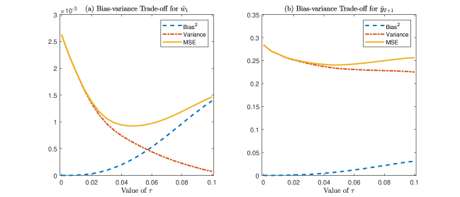
Figure S1: The Bias and Variance Trade-off under Different $\tau$ Values

Figure S1 demonstrates the bias and variance trade-off under a range of $\tau$ in a simulated numerical example. Let

$$y_{t+1}=\sum_{i=1}^{20}w_{i}f_{it}+u_{t+1},\ \ t=1,\ldots,100.$$

The dependent variable $y_{t+1}$ is a linear combination of two groups of input variables $\{f_{it}\}_{i=1}^{10}$ and $\{f_{it}\}_{i=11}^{20}$ with group weights

$$w_{i}=0.09\cdot 1\left\{1\leq i\leq 10\right\}+0.01\cdot 1\left\{11\leq i\leq 20\right\}$$

so that $\sum_{i=1}^{20}w_{i}=1$. We set $f_{it}\sim\mbox{i.i.d.\,}N(1,1)$ for $1\leq i\leq 10$, $f_{it}\sim\mbox{i.i.d.\,}N(0,1)$ for $11\leq i\leq 20$, and $u_{t+1}\sim\mbox{i.i.d.\,}N(0,0.25)$. We estimate the weights by $\ell_{2}$-relaxation under different values of $\tau=0,0.005,0.01,\ldots,0.1$. Let $\widehat{w}_{1}=\widehat{w}_{1\tau}$ denote the first element of the $\ell_{2}$-relaxation estimator $\mathbf{\widehat{w}}_{\tau}.$

We report in Figure S1 the empirical squared bias, variance and MSE of $(\widehat{w}_{1}=\widehat{w}_{1\tau})$ and those of the one-step-ahead forecast $\widehat{y}_{102}$ over 1000 replications as a function of $\tau$. The figure shows that both the $\ell_{2}$-relaxation weight estimator and the one-step-ahead forecast associated with a small value of $\tau$ have small biases but large variances whereas those associated with a large value of $\tau$ have large biases but small variances. In the middle, there is a wide range of values of $\tau$ where the combined forecast yields smaller MSFE than either that of the simple average estimator (when $\tau$ is sufficiently large) or that of the classical optimal weight $\widehat{\mathbf{w}}^{\mathrm{C}}$ (when $\tau=0$).

B.2 SNR in the Section 4

To calculate the signal-to-noise ratio (SNR) in the simulations, we decompose $y_{t+1}=\mathbf{w}_{\psi}^{\ast\prime}\left(\mathbf{f}_{t}-\mathbf{u}_{t}\right)+u_{y,t+1}$ into

$$y_{t+1}=\underbrace{\mathbf{w}_{\psi}^{\ast\prime}\left(\mathbf{f}_{t}-\mathcal{P}\left[\mathbf{u}_{t}|\mathbf{f}_{t}\right]\right)}_{\mathrm{signal}}-\underbrace{\mathbf{w}_{\psi}^{\ast\prime}\left(\mathbf{u}_{t}-\mathcal{P}\left[\mathbf{u}_{t}|\mathbf{f}_{t}\right]\right)+u_{y,t+1}}_{\mathrm{noise}},$$

where $\mathcal{P}\left[\mathbf{u}_{t}|\mathbf{f}_{t}\right]:=E\left[\mathbf{u}_{t}\mathbf{f}_{t}^{\prime}\right]\left(E\left[\mathbf{f}_{t}\mathbf{f}_{t}^{\prime}\right]\right)^{-1}\mathbf{f}_{t}=\mathbf{\Omega}_{u}\left(\mathbf{\Psi}+\mathbf{\Omega}_{u}\right)^{-1}\mathbf{f}_{t}$ is the linear projection of $\mathbf{u}_{t}$ onto the linear space spanned by $\mathbf{f}_{t}$. By construction, the signal and noise terms are orthogonal in that

$$E\left[\mathbf{w}_{\psi}^{\ast\prime}\left(\mathbf{f}_{t}-\mathcal{P}\left[\mathbf{u}_{t}|\mathbf{f}_{t}\right]\right)\left(\mathbf{u}_{t}-\mathcal{P}\left[\mathbf{u}_{t}|\mathbf{f}_{t}\right]\right)^{\prime}\mathbf{w}_{\psi}^{\ast}\right]$$

$$= \mathbf{w}_{\psi}^{\ast\prime}E\left[\left(\mathbf{f}_{t}-\mathbf{\Omega}_{u}\left(\mathbf{\Psi}+\mathbf{\Omega}_{u}\right)^{-1}\mathbf{f}_{t}\right)\left(\mathbf{u}_{t}-\mathbf{\Omega}_{u}\left(\mathbf{\Psi}+\mathbf{\Omega}_{u}\right)^{-1}\mathbf{f}_{t}\right)^{\prime}\right]\mathbf{w}_{\psi}^{\ast}=0.$$

Simple calculation shows that the variance of the noise component is

$$\mathrm{var}\left[\mathbf{w}_{\psi}^{\ast\prime}\left(\mathbf{u}_{t}-\mathcal{P}\left[\mathbf{u}_{t}|\mathbf{f}_{t}\right]\right)+u_{y,t+1}\right]=\mathbf{w}_{\psi}^{\ast\prime}\left[\mathbf{\Omega}_{u}-\mathbf{\Omega}_{u}\left(\mathbf{\Psi}+\mathbf{\Omega}_{u}\right)^{-1}\mathbf{\Omega}_{u}\right]\mathbf{w}_{\psi}^{\ast}+\sigma_{y}^{2}\text{.}$$

This, along with the fact that $\mathrm{var}[y_{t+1}]=\mathbf{w}_{\psi}^{\ast\prime}\mathbf{\Psi}\mathbf{w}_{\psi}^{\ast}+\sigma_{y}^{2},$ implies that SNR here can be defined as

$$\mathrm{SNR} = \frac{\mathrm{var}[y_{t+1}]-\mathrm{var}\left[\mathbf{w}_{\psi}^{\ast\prime}\left(\mathbf{u}_{t}-\mathcal{P}\left[\mathbf{u}_{t}|\mathbf{f}_{t}\right]\right)+u_{y,t+1}\right]}{\mathrm{var}\left[\mathbf{w}_{\psi}^{\ast\prime}\left(\mathbf{u}_{t}-\mathcal{P}\left[\mathbf{u}_{t}|\mathbf{f}_{t}\right]\right)+u_{y,t+1}\right]}$$

$$= \frac{\mathbf{w}_{\psi}^{\ast\prime}\left[\mathbf{\Psi-\Omega}_{u}+\mathbf{\Omega}_{u}\left(\mathbf{\Psi}+\mathbf{\Omega}_{u}\right)^{-1}\mathbf{\Omega}_{u}\right]\mathbf{w}_{\psi}^{\ast}}{\mathbf{w}_{\psi}^{\ast\prime}\left[\mathbf{\Omega}_{u}-\mathbf{\Omega}_{u}\left(\mathbf{\Psi}+\mathbf{\Omega}_{u}\right)^{-1}\mathbf{\Omega}_{u}\right]\mathbf{w}_{\psi}^{\ast}+\sigma_{y}^{2}}.$$

B.3 Simulation Results for DGP 2 by Using the 5-fold CV

Table S1 reports the MSFEs for DGP 2 by using the conventional 5-fold CV to choose $\tau$ as in Box 2. Note that only Lasso, Ridge, and $\ell_{2}$-relaxation depend on tuning parameters. The results of other estimators with no data-driven tuning parameters are the same as those in Panel C and D of Table 1. We find that MSFEs from the 5-fold CV generally provides outcomes slightly better than the time series CV as in Box 3. In theory, both the randomly formed CV folds and the time series CV folds allow consistent estimation of VC from the training data as $T\rightarrow\infty$. In practice, however, the former uses $4/5$ of the sample for training in each fold, while the latter utilizes $1/5,2/5,3/5,4/5$ respectively for each fold. The smaller practical training data sample sizes in the time series scheme tend to yield more noisy VC estimates, and thereby larger MSFEs in Table 1.

Table S1: The MSFE for DGP 2 by Using the 5-fold CV

	$T$	$N$	$K$	Oracle	SA	Lasso	Ridge	PC				$\ell_{2}$-relax
								$q=5$	$q=10$	$q=20$		$\widehat{\boldsymbol{\Sigma}}_{s}$	$\widehat{\boldsymbol{\Sigma}}_{1}$	$\widehat{\boldsymbol{\Sigma}}_{2}$
Panel A: Low SNR
	50	100	2	0.292	1.032	0.404	1.131	0.787	0.800	0.763		0.386	0.390	0.364
	100	200	4	0.133	3.052	0.232	1.090	1.134	1.275	1.531		0.219	0.232	0.265
	200	300	6	0.066	3.699	0.141	0.398	1.109	1.050	1.173		0.114	0.124	0.082
Panel B: High SNR
	50	100	2	0.262	0.993	0.394	1.387	0.702	0.747	0.751		0.282	0.305	0.267
	100	200	4	0.146	3.210	0.370	1.376	1.030	1.257	1.428		0.292	0.281	0.315
	200	300	6	0.106	4.524	0.162	0.430	1.343	1.601	1.639		0.177	0.193	0.167

B.4 MAFE for the Simulations

In this section we report the mean absolute forecast error (MAFE) in the simulations. The MAFE is defined as

$$\text{MAFE}=E\left[\left|y_{T+1}-\widehat{\mathbf{w}}^{\prime}\mathbf{f}_{T+1}\right|\right]-\sigma_{y}\sqrt{2/\pi},$$

where the unpredictable component, $\sigma_{y}\int_{-\infty}^{\infty}|x|\frac{1}{\sqrt{2\pi}}\exp(-x^{2}/2)\mathrm{d}x=\sigma_{y}\sqrt{2/\pi}$, is subtracted. In simulations we know $\sigma_{y}$ albeit it is unknown in empirical applications.

The results are collected in Table S2. Results by the Oracle, Lasso, Ridge, and the $\ell_{2}$-relaxation tend to decrease with $\left({T,N}\right)$, yet results by SA and PC may diverge as $\left({T,N}\right)$ increases. Similar to the MSFE results in the main text, the $\ell_{2}$-relaxation is always the best feasible estimator in all cases.

Table S2: Results of Prediction Accuracy by MAFE

	$T$	$N$	$K$	Oracle	SA	Lasso	Ridge	PC			$\ell_{2}$-relax
								$q=5$	$q=10$	$q=20$	$\hat{\Sigma}_{0}$	$\hat{\Sigma}_{1}$	$\hat{\Sigma}_{2}$
Panel A: DGP1 with Low SNR
	50	100	2	0.125	0.318	0.160	0.413	0.242	0.248	0.232	0.154	0.143	0.135
	100	200	4	0.063	0.949	0.098	0.323	0.370	0.440	0.436	0.089	0.090	0.087
	200	300	6	0.034	1.063	0.055	0.142	0.386	0.439	0.423	0.054	0.050	0.043
Panel B: DGP1 with High SNR
	50	100	2	0.337	0.696	0.381	0.497	0.586	0.596	0.586	0.351	0.349	0.344
	100	200	4	0.221	1.267	0.255	0.339	0.695	0.765	0.801	0.234	0.234	0.229
	200	300	6	0.182	1.510	0.210	0.222	0.790	0.802	0.805	0.205	0.206	0.197
Panel C: DGP2 with Low SNR
	50	100	2	0.104	0.318	0.137	0.407	0.250	0.252	0.253	0.140	0.139	0.131
	100	200	4	0.063	0.820	0.097	0.320	0.366	0.389	0.467	0.091	0.102	0.117
	200	300	6	0.020	0.917	0.048	0.138	0.348	0.329	0.366	0.061	0.050	0.048
Panel D: DGP2 with High SNR
	50	100	2	0.336	0.718	0.386	0.474	0.590	0.615	0.611	0.349	0.351	0.344
	100	200	4	0.231	1.361	0.272	0.348	0.715	0.782	0.845	0.248	0.254	0.241
	200	300	6	0.192	1.589	0.214	0.231	0.826	0.906	0.907	0.209	0.208	0.199
Panel E: DGP3 with Low SNR
	50	100	2	0.160	0.350	0.345	0.477	0.291	0.324	0.305	0.191	0.179	0.162
	100	200	4	0.102	0.949	0.238	0.443	0.517	0.520	0.581	0.122	0.135	0.116
	200	300	6	0.098	1.105	0.181	0.278	0.553	0.619	0.662	0.101	0.117	0.107
Panel F: DGP3 with High SNR
	50	100	2	0.420	0.775	0.620	0.626	0.683	0.706	0.717	0.442	0.440	0.429
	100	200	4	0.348	1.373	0.436	0.483	0.896	0.939	0.978	0.367	0.352	0.353
	200	300	6	0.338	1.635	0.380	0.405	1.046	1.064	1.101	0.359	0.368	0.347

B.5 MAFE for the Empirical Applications

Tables S3 and S4 report the relative (to the benchmark) MAFEs in the movie and HICP forecasting applications, respectively. The results and patterns are robust in comparison with those based on MSFE.

Table S3: Relative MAFE of Movie Forecasting

$n_{\mathrm{ev}}$	PMA	CSR10	CSR15	peLasso	Lasso	Ridge	$\ell_{2}$-relax
							$\widehat{\boldsymbol{\Sigma}}_{s}$	$\widehat{\boldsymbol{\Sigma}}_{1}$	$\widehat{\boldsymbol{\Sigma}}_{2}$
10	1.000	1.144	1.164	2.707	1.013	1.018	0.984	0.985	0.983
20	1.000	1.139	1.189	2.610	1.024	1.030	0.985	0.988	0.985
30	1.000	1.068	1.138	2.432	1.019	1.039	0.984	0.982	0.980
40	1.000	1.013	1.098	2.269	1.008	1.039	0.995	0.990	0.970
Note: The MAFE of PMA is normalized as 1.

Table S4: Relative MAFE of HICP Forecasting

Horizon	SA	Lasso	Ridge	$\ell_{2}$-relax
				$\widehat{\boldsymbol{\Sigma}}_{s}$	$\widehat{\boldsymbol{\Sigma}}_{1}$	$\widehat{\boldsymbol{\Sigma}}_{2}$
One-year-ahead	1.000	0.909	0.922	0.933	0.847	0.885
Two-year-ahead	1.000	0.828	0.924	0.817	0.850	0.756
Note: The MAFE of SA is normalized as 1.

B.6 Converging Path of Weights

In this section, we estimate the weights of the $\ell_{2}$-relaxation estimator over different values of $\tau$ and compare the converging path with the Ridge weights. The data is generated from DGP 1 in the simulation with 50 observations and 100 forecasters that are categorized into two latent groups. The two subplots of Figure S2 illustrate the converging paths of the $\ell_{2}$-relaxation and Ridge weights over different values of $\tau$, respectively. The horizontal axis represents the values of $\tau$ and the vertical axis shows the values of weights for the 100 forecasters.

When $\tau=0$, all the weights are scattered. As $\tau$ increases, the $\ell_{2}$-relaxation weights quickly converge to two group centers, which can be clearly observed for $\tau\in[1,3.5]$. When $\tau>3.5$, the tuning parameter is so large that the weights converge to the simple average (SA) weights $1/N$. In contrast, the Ridge weights do not converge to two group clusters even though they are centered around the SA weights.

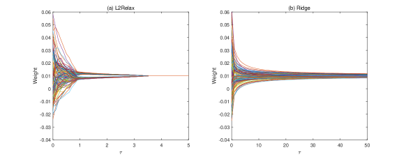
Figure S2: Converging Path of Weights over Different Values of $\tau$

References

• Ang et al. (2007) Ang, A., G. Bekaert, and M. Wei (2007). Do macro variables, asset markets, or surveys forecast inflation better? Journal of Monetary Economics 54(4), 1163–1212.
• Ao et al. (2019) Ao, M., Y. Li, and X. Zheng (2019). Approaching mean-variance efficiency for large portfolios. The Review of Financial Studies 32(7), 2890–2919.
• Arlot and Celisse (2010) Arlot, S. and A. Celisse (2010). A survey of cross-validation procedures for model selection. Statistcs Surveys 4, 40–79.
• Bates and Granger (1969) Bates, J. M. and C. W. Granger (1969). The combination of forecasts. Operational Research Quarterly 20, 451–468.
• Bayer (2018) Bayer, S. (2018). Combining value-at-risk forecasts using penalized quantile regressions. Econometrics and Statistics 8, 56–77.
• Belloni et al. (2012) Belloni, A., D. Chen, V. Chernozhukov, and C. Hansen (2012). Sparse models and methods for optimal instruments with an application to eminent domain. Econometrica 80, 2369–2429.
• Bergmeir and Benítez (2012) Bergmeir, C. and J. M. Benítez (2012). On the use of cross-validation for time series predictor evaluation. Information Sciences 191, 192 – 213. Data Mining for Software Trustworthiness.
• Bergmeir et al. (2018) Bergmeir, C., R. J. Hyndman, and B. Koo (2018). A note on the validity of cross-validation for evaluating autoregressive time series prediction. Computational Statistics & Data Analysis 120, 70–83.
• Bickel et al. (2009) Bickel, P., Y. Ritov, and A. Tsybakov (2009). Simultaneous analysis of Lasso and Dantzig selector. The Annals of Statistics 37(4), 1705–1732.
• Bickel and Levina (2008) Bickel, P. J. and E. Levina (2008). Regularized estimation of large covariance matrices. The Annals of Statistics 36(1), 199–227.
• Bonhomme et al. (2022) Bonhomme, S., T. Lamadon, and E. Manresa (2022). Discretizing unobserved heterogeneity. Econometrica 90(2), 625–643.
• Bonhomme and Manresa (2015) Bonhomme, S. and E. Manresa (2015). Grouped patterns of heterogeneity in panel data. Econometrica 83(3), 1147–1184.
• Boyd and Vandenberghe (2004) Boyd, S. and L. Vandenberghe (2004). Convex optimization. Cambridge University Press.
• Bühlmann and van de Geer (2011) Bühlmann, P. and S. van de Geer (2011). Statistics for High-Dimensional Data: Methods, Theory and Applications. Springer.
• Cai et al. (2020) Cai, T. T., J. Hu, Y. Li, and X. Zheng (2020). High-dimensional minimum variance portfolio estimation based on high-frequency data. Journal of Econometrics 214(2), 482–494.
• Candes and Tao (2007) Candes, E. and T. Tao (2007). The Dantzig selector: Statistical estimation when $p$ is much larger than $n$. The Annals of Statistics 35(6), 2313–2351.
• Chan and Pauwels (2018) Chan, F. and L. L. Pauwels (2018). Some theoretical results on forecast combinations. International Journal of Forecasting 34(1), 64–74.
• Chetverikov et al. (2021) Chetverikov, D., Z. Liao, and V. Chernozhukov (2021). On cross-validated lasso in high dimensions. The Annals of Statistics 49(3), 1300–1317.
• Claeskens et al. (2016) Claeskens, G., J. R. Magnus, A. L. Vasnev, and W. Wang (2016). The forecast combination puzzle: A simple theoretical explanation. International Journal of Forecasting 32(3), 754–762.
• Clemen (1989) Clemen, R. T. (1989). Combining forecasts: A review and annotated bibliography. International Journal of forecasting 5(4), 559–583.
• Clements et al. (2015) Clements, A., A. Scott, and A. Silvennoinen (2015). On the benefits of equicorrelation for portfolio allocation. Journal of Forecasting 34(6), 507–522.
• Conflitti et al. (2015) Conflitti, C., C. De Mol, and D. Giannone (2015). Optimal combination of survey forecasts. International Journal of Forecasting 31(4), 1096–1103.
• Coulombe et al. (2020) Coulombe, P. G., M. Leroux, D. Stevanovic, and S. Surprenant (2020). How is machine learning useful for macroeconomic forecasting? Technical report, CIRANO.
• DeMiguel et al. (2009) DeMiguel, V., L. Garlappi, F. J. Nogales, and R. Uppal (2009). A generalized approach to portfolio optimization: Improving performance by constraining portfolio norms. Management Science 55(5), 798–812.
• DeMiguel et al. (2009) DeMiguel, V., L. Garlappi, and R. Uppal (2009). Optimal versus naive diversification: How inefficient is the 1/n portfolio strategy? The review of Financial studies 22(5), 1915–1953.
• Diebold and Shin (2019) Diebold, F. X. and M. Shin (2019). Machine learning for regularized survey forecast combination: Partially-egalitarian lasso and its derivatives. International Journal of Forecasting 35(4), 1679–1691.
• Diebold et al. (2022) Diebold, F. X., M. Shin, and B. Zhang (2022). On the aggregation of probability assessments: Regularized mixtures of predictive densities for eurozone inflation and real interest rates. Working Paper, National Bureau of Economic Research.
• Ding et al. (2021) Ding, Y., Y. Li, and X. Zheng (2021). High dimensional minimum variance portfolio estimation under statistical factor models. Journal of Econometrics 222(1), 502–515.
• Disatnik and Katz (2012) Disatnik, D. and S. Katz (2012). Portfolio optimization using a block structure for the covariance matrix. Journal of Business Finance & Accounting 39(5-6), 806–843.
• Elliott et al. (2013) Elliott, G., A. Gargano, and A. Timmermann (2013). Complete subset regressions. Journal of Econometrics 177(2), 357–373.
• Elliott and Timmermann (2016) Elliott, G. and A. Timmermann (2016). Economic Forecasting. Princeton University Press.
• Engle and Kelly (2012) Engle, R. and B. Kelly (2012). Dynamic equicorrelation. Journal of Business & Economic Statistics 30(2), 212–228.
• Fama and French (2015) Fama, E. F. and K. R. French (2015). A five-factor asset pricing model. Journal of Financial Economics 116(1), 1 – 22.
• Fan et al. (2016) Fan, J., A. Furger, and D. Xiu (2016). Incorporating global industrial classification standard into portfolio allocation: A simple factor-based large covariance matrix estimator with high-frequency data. Journal of Business & Economic Statistics 34(4), 489–503.
• Fan and Li (2001) Fan, J. and R. Li (2001). Variable selection via nonconcave penalized likelihood and its oracle properties. Journal of the American Statistical Association 96(456), 1348–1360.
• Fan et al. (2012) Fan, J., Y. Li, and K. Yu (2012). Vast volatility matrix estimation using high-frequency data for portfolio selection. Journal of the American Statistical Association 107(497), 412–428.
• Fan et al. (2016) Fan, J., Y. Liao, and H. Liu (2016). An overview of the estimation of large covariance and precision matrices. The Econometrics Journal 19(1), C1–C32.
• Fan et al. (2013) Fan, J., Y. Liao, and M. Mincheva (2013). Large covariance estimation by thresholding principal orthogonal complements. Journal of the Royal Statistical Society: Series B (Statistical Methodology) 75(4), 603–680.
• Fan et al. (2012) Fan, J., J. Zhang, and K. Yu (2012). Vast portfolio selection with gross-exposure constraints. Journal of the American Statistical Association 107(498), 592–606.
• Gao and Shi (2020) Gao, Z. and Z. Shi (2020). Implementing convex optimization in r: Two econometric examples. Computational Economics.
• Genre et al. (2013) Genre, V., G. Kenny, A. Meyler, and A. Timmermann (2013). Combining expert forecasts: Can anything beat the simple average? International Journal of Forecasting 29(1), 108 – 121.
• Granger and Ramanathan (1984) Granger, C. W. and R. Ramanathan (1984). Improved methods of combining forecasts. Journal of Forecasting 3(2), 197–204.
• Grant and Boyd (2014) Grant, M. and S. Boyd (2014). CVX: Matlab software for disciplined convex programming, version 2.1. http://cvxr.com/cvx.
• Gu et al. (2020) Gu, S., B. Kelly, and D. Xiu (2020). Empirical asset pricing via machine learning. Review of Financial Studies 33(5), 2223–2273.
• Hansen (2007) Hansen, B. E. (2007). Least squares model averaging. Econometrica 75(4), 1175–1189.
• Hsiao and Wan (2014) Hsiao, C. and S. K. Wan (2014). Is there an optimal forecast combination? Journal of Econometrics 178, 294–309.
• Jagannathan and Ma (2003) Jagannathan, R. and T. Ma (2003). Risk reduction in large portfolios: Why imposing the wrong constraints helps. The Journal of Finance 58(4), 1651–1683.
• Kotchoni et al. (2019) Kotchoni, R., M. Leroux, and D. Stevanovic (2019). Macroeconomic forecast accuracy in a data-rich environment. Journal of Applied Econometrics 34(7), 1050–1072.
• Ledoit and Wolf (2004) Ledoit, O. and M. Wolf (2004). Honey, I shrunk the sample covariance matrix. The Journal of Portfolio Management 30(4), 110–119.
• Ledoit and Wolf (2017) Ledoit, O. and M. Wolf (2017). Nonlinear shrinkage of the covariance matrix for portfolio selection: Markowitz meets goldilocks. The Review of Financial Studies 30(12), 4349–4388.
• Ledoit and Wolf (2020) Ledoit, O. and M. Wolf (2020). Analytical nonlinear shrinkage of large-dimensional covariance matrices. The Annals of Statistics 48(5), 3043 – 3065.
• Lehrer and Xie (2017) Lehrer, S. F. and T. Xie (2017). Box office buzz: does socialmedia data steal the show from model uncertainty when forecasting for hollywood? The Review of Economics and Statistics 99(5), 749–755.
• Linton (2019) Linton, O. (2019). Financial Econometrics: Models and Methods. Cambridge University Press.
• Markowitz (1952) Markowitz, H. (1952). Portfolio selection. The Journal of Finance 7(1), 77–91.
• Merton (1980) Merton, R. C. (1980). On estimating the expected return on the market: An exploratory investigation. Journal of Financial Economics 8(4), 323–361.
• Mirakyan et al. (2017) Mirakyan, A., M. Meyer-Renschhausen, and A. Koch (2017). Composite forecasting approach, application for next-day electricity price forecasting. Energy Economics 66, 228 – 237.
• Rényi (1961) Rényi, A. (1961). On measures of entropy and information. In Proceedings of the fourth Berkeley symposium on mathematical statistics and probability, Volume 1. Berkeley, California, USA.
• Roccazzella et al. (2020) Roccazzella, F., P. Gambetti, and F. Vrins (2020). Optimal and robust combination of forecasts via constrained optimization and shrinkage. Technical report, LFIN Working Paper Series, 2020/6, 1–2.
• Shi (2016) Shi, Z. (2016). Econometric estimation with high-dimensional moment equalities. Journal of Econometrics 195(1), 104–119.
• Smith and Wallis (2009) Smith, J. and K. F. Wallis (2009). A simple explanation of the forecast combination puzzle. Oxford Bulletin of Economics and Statistics 71(3), 331–355.
• Stock and Watson (2004) Stock, J. H. and M. W. Watson (2004). Combination forecasts of output growth in a seven-country data set. Journal of Forecasting 23(6), 405–430.
• Su and Ju (2018) Su, L. and G. Ju (2018). Identifying latent grouped patterns in panel data models with interactive fixed effects. Journal of Econometrics 206(2), 554–573.
• Su et al. (2016) Su, L., Z. Shi, and P. C. Phillips (2016). Identifying latent structures in panel data. Econometrica 84(6), 2215–2264.
• Su et al. (2019) Su, L., X. Wang, and S. Jin (2019). Sieve estimation of time-varying panel data models with latent structures. Journal of Business & Economic Statistics 37(2), 334–349.
• Tibshirani (1996) Tibshirani, R. (1996). Regression shrinkage and selection via the lasso. Journal of the Royal Statistical Society. Series B (Methodological), 267–288.
• Vogt and Linton (2017) Vogt, M. and O. Linton (2017). Classification of non-parametric regression functions in longitudinal data models. Journal of the Royal Statistical Society: Series B (Statistical Methodology) 79(1), 5–27.
• Vogt and Linton (2020) Vogt, M. and O. Linton (2020). Multiscale clustering of nonparametric regression curves. Journal of Econometrics.
• Wainwright (2019) Wainwright, M. J. (2019). High-dimensional statistics: A non-asymptotic viewpoint, Volume 48. Cambridge University Press.
• Wang and Su (2021) Wang, W. and L. Su (2021). Identifying latent group structures in nonlinear panels. Journal of Econometrics 220(2), 272–295.
• Wilms et al. (2018) Wilms, I., J. Rombouts, and C. Croux (2018). Multivariate lasso-based forecast combinations for stock market volatility. Working paper, Faculty of Economics and Business, KU Leuven.
• Wu and Wang (2020) Wu, Y. and L. Wang (2020). A survey of tuning parameter selection for high-dimensional regression. Annual Review of Statistics and Its Application 7, 209–226.
• Zou and Hastie (2005) Zou, H. and T. Hastie (2005). Regularization and variable selection via the elastic net. Journal of the Royal Statistical Society: series B (Statistical Methodology) 67(2), 301–320.
Online Supplement for