Unsupervised Expressive Rules Provide Explainability and
Assist Human Experts Grasping New Domains

Abstract

Approaching new data can be quite deterrent; you do not know how your categories of interest are realized in it, commonly, there is no labeled data at hand, and the performance of domain adaptation methods is unsatisfactory.

Aiming to assist domain experts in their first steps into a new task over a new corpus, we present an unsupervised approach to reveal complex rules which cluster the unexplored corpus by its prominent categories (or facets).

These rules are human-readable, thus providing an important ingredient which has become in short supply lately - explainability. Each rule provides an explanation for the commonality of all the texts it clusters together.

We present an extensive evaluation of the usefulness of these rules in identifying target categories, as well as a user study which assesses their interpretability.

1 Introduction

A common scenario faced by subject matter experts tackling a new text understanding task is getting to know a new dataset, for which there is no labeled data. Understanding the unexplored data, and collecting first insights from it, is always a slow process. Often, the expert is trying to categorize the data, and potentially build a system to automatically identify these categories. For example, an expert may be looking at customer complaints, aiming to understand their types or categories, and then building a system that will categorize complaints. Or she may be analyzing contracts, aiming to identify the types of legal commitments.

In other cases, the expert may be trying to identify a certain class of texts, and this class may be composed of unknown underlying sub-types or categories. Consider a data scientist looking for all arguments, related to a suggested policy, raised in a public participation forum. These arguments may be of several types, which are a-priori unknown.

When facing a new task, with no labeled data, but with domain expertise, a practical first step is to manually write rules that identify some texts from a certain category the expert is aware of and aiming to identify (e.g., a certain complaint type). With these seed examples, experts can better understand the occurrences of the target category in the new corpus, and use them as the initial set of labeled examples, towards the goal of having enough labeled data to facilitate supervised learning.

However, oftentimes, the categories underlying the data are not known a-priori, and may be a part of what the expert aims to identify (e.g., what are the types of complaints). Since new data may mean new underlying categories, domain adaptation is not always applicable, and often results in unsatisfying performance Ziser and Reichart (2018).

Dataset-category	No.	Sentences Matched	Rule
ASRD argument	1 2 3	so first let us address the question our second argument is about my first overview is	[hyponym of rank] $+$ [WordNet super class of communication] (an ordinal number, a term relating to human communication)
ASRD argument	4 5 6	additionally I think that sam is confused ultimately, we think that it limits the obviously, we acknowledge it’s important	[adverb] $+$ [personal pronoun] $+$ [hyponym of think] $+$ [sentiment word] (an adverb, an indication of a person, a term related to thinking, and a word bearing a clear sentiment)
Essays premise	7 8 9	for example, employer always prefer to for instance, several teenagers play games as a matter of fact, women have proved	[preposition] + [hyponym of psychological feature] + [hyponym of causal agent] (a preposition, a term related to the mental domain, and an entity that can cause a change of any type)
HOLJ background	10 11 12	Section 171B ( 1 ) provides : ” ( 1 ) This section applies where - Paragraph 11 of the circular states :	[hyponym of written communication] + [noun] + [Verb, 3rd person singular present] (a written entity, followed by a noun, and a verb for he/she/it in present tense)
ToS unfair clauses	13 14 15	we may take any of these actions at any time suspend your access to any of the no liability to you or any third party	[ndet syntactic relation] + [any] (a noun determiner, followed by the word “any”)

Table 1: Examples for rules and generalizations found. Matched words are in bold. A description of each rule is provided below it, in parentheses. The datasets and categories are described in Section 3.

In this paper, we present a method for generating initial rules automatically, with no need for any labeled data, nor for a list of categories.

Our method, GrASP${}^{\hskip 1.0pt{\textrm{{lite}}}}$, is based on GrASP Shnarch et al. (2017). GrASP is a supervised algorithm that finds highly expressive rules, in the form of patterns, that capture the common structures of a category of interest. GrASP requires a set of texts in which the target category appears and a set in which it does not. GrASP${}^{\hskip 1.0pt{\textrm{{lite}}}}$ is an unsupervised version of GrASP, that requires no labeled data and no prior knowledge.

Instead, GrASP${}^{\hskip 1.0pt{\textrm{{lite}}}}$ takes a background corpus and contrasts it with the new corpus, the foreground corpus. By this, it reveals rules which capture sentences that are common in the foreground but not in the background. Such sentences are expected to be correlated with (at least some of) the unique categories in the foreground – the new corpus. Examples of such rules are given in Table 1.

Naturally, rules generated without supervision would be noisy. In addition, the rules revealed by GrASP${}^{\hskip 1.0pt{\textrm{{lite}}}}$ capture a mixture of the categories that exist in the foreground corpus, some of which may be irrelevant for the task at hand. We, therefore, suggest GrASP${}^{\hskip 1.0pt{\textrm{{lite}}}}$ as a preliminary automatic step which provides input for the human expert, without any input needed beyond the corpus of text. As rules are human-readable, and each one provides an explanation for why it clusters sentences together, experts can identify the subset of rules which, together, best capture the sentences of their category of interest. Experts can also be inspired by the rules suggested by GrASP${}^{\hskip 1.0pt{\textrm{{lite}}}}$, manually edit rules to better fit their needs, merge elements from several rules into new rules, or improve their own manual rules with generalizations offered by the suggested rules. In other words, GrASP${}^{\hskip 1.0pt{\textrm{{lite}}}}$ is a way to alleviate the blank canvas problem and to expedite the expert’s work.

The rules identified by GrASP${}^{\hskip 1.0pt{\textrm{{lite}}}}$ not only elucidate the underlying categories and facilitate rule-based algorithms, but also provide the benefit of explainability. That is, the human expert can now explain why a text is classified as a complaint and why it is in a certain complaint category.

We extensively evaluate GrASP${}^{\hskip 1.0pt{\textrm{{lite}}}}$ over datasets from different domains, and show that the rules it generates, without being exposed to the datasets’ categories, can help identify these categories. We further present a user study which validates the explainability power of GrASP${}^{\hskip 1.0pt{\textrm{{lite}}}}$ rules.

2 GrASP${}^{\hskip 1.0pt{\textrm{{lite}}}}$

When facing a new task with new data, it is useful to have a tool which can quickly highlight some interesting aspects of these data. Such a tool must work with minimal prerequisites, as often we have little information about the new data.

This is what our proposed method, GrASP${}^{\hskip 1.0pt{\textrm{{lite}}}}$, aims to provide. GrASP${}^{\hskip 1.0pt{\textrm{{lite}}}}$ is based on GrASP Shnarch et al. (2017), an algorithm for extracting highly expressive rules, in the form of patterns, for detecting a target category in texts.

A good rule is one that captures different realizations of the target category. For example, humans reading 1–3 in Table 1 can notice their commonality, even if they cannot name it. GrASP offers a rule which generalizes these realizations, and reveals their common structure: a hyponym of the noun rank, closely followed by a noun which is a descendant, in WordNet, of communication.

To achieve this goal, GrASP extracts patterns that characterize a target linguistic phenomenon (e.g., argumentative sentences). Its input is a set of positive examples (in which the phenomenon appears) and another set of negative examples (in which it does not). First, all terms of all examples are augmented with a variety of linguistic attributes. Attributes are any type of term-level information, such as syntactic information (e.g., part-of-speech tag, information from the parsed tree), semantic (e.g., is the term a named entity? what are its hypernyms?), task-specific (e.g., is the term included in a relevant lexicon?), and more. Next, GrASP greedily selects top attributes according to their information gain with the label. These attributes make the alphabet. Patterns are grown in iterations by combining attributes of the alphabet with shorter patterns from the previous iteration. At the end of each iteration a greedy step keeps only the top patterns (by information gain).

In this work, we use a commonly available attribute set, which includes the surface form of the term, POS tags, Named Entity Recognizer, WordNet Miller (1998), and a sentiment lexicon. We used the same set of attributes throughout our experiments, but one can add specific ones or rely on different technologies to extract them (e.g., a new parsing technology). See rule examples in Table 1.

As the rules are human-readable and expose common structures in the data, they can expedite the process of getting to know it, especially when addressing novel domains.

An entry barrier is that GrASP requires labeled data which may not be available for a new domain. GrASP${}^{\hskip 1.0pt{\textrm{{lite}}}}$ aims to lift this barrier by providing a method to generate the two input sets for GrASP, with no labeled data. It achieves that by setting a more modest goal – instead of discovering rules describing common structures of a target category, GrASP${}^{\hskip 1.0pt{\textrm{{lite}}}}$ aims to discover rules describing non-trivial structures which capture some repeating meaning, or category. However, these rules must not overfit the available data.

To achieve this goal, GrASP${}^{\hskip 1.0pt{\textrm{{lite}}}}$ contrasts the available data, the foreground corpus (which serves as the positive set), with a background corpus (used as the negative set) in which the categories of interest are expected to be significantly less prominent. With these two input sets, the regular GrASP can be applied. By the nature of weak supervision, the foreground is not guaranteed to contain only positive examples (same for background and negative). However, we hypothesize that it is enough for a phenomenon to be more prominent in the foreground than it is in the background, for the regular GrASP to extract rules that characterize it. This way, by discovering rules for repeating meaningful structures which tend to appear in the foreground corpus more than in the background corpus, GrASP${}^{\hskip 1.0pt{\textrm{{lite}}}}$ describes the common and unique categories of the available data. Next, we describe two methods to obtain a background corpus.

General English

A simple choice is to take random texts of the language of interest. We sampled 50,000 sentences from a news-domain corpus. In many cases, such a corpus is, on the one hand, different enough from the domain corpus (so can be assumed to be less enriched with the target category), and on the other hand, similar enough so as not to make the discrimination task of GrASP${}^{\hskip 1.0pt{\textrm{{lite}}}}$ trivial (which will result in non-informative rules).

However, in other cases, such a random sample of texts would not yield a suitable background corpus. For a distinctive domain corpus, legal contracts for example, contrasting it with a general English background will mostly bring up the legal jargon which is very common in the domain and rare in general English. The structures of legal commitments, a potential target category, would be obscured by this specificity of the domain. Thus, another method is needed, one which builds a background corpus from the domain corpus itself.

In-Domain Split

For those cases, in which a general English background is too distinct from the foreground corpus, we suggest splitting the domain corpus itself into foreground and background. In this in-domain split the language style in the foreground and the background are similar, thus it avoids the risk of discovering rules that simply capture stylistic differences between the two parts.

If the expert has some knowledge about the new domain, it can be used to come up with a heuristic to split the new corpus. As an example of knowledgeable in-domain split we take the argument mining task. Argumentative sentences, aiming to persuade, ought to be well structured, to be easily understood by an audience, and often include foreshadowing hints, to guide the audience through the full argument. We hypothesize that such structures are more likely to be found in the beginning of a sentence, rather than in its end. Based on this hypothesis, the foreground is made of the first halves of all sentences in the corpus, while the background is made of the second halves. We used this split method as an example in the analysis in §5.3.

If no heuristic can be found for the dataset, we suggest splitting it based on an unsupervised clustering method. The expert examines the clusters and chooses as the foreground one cluster which seems to contain many sentences of the target category. This selection does not have to be optimal (i.e., choosing the cluster with the most relevant sentences). It is enough that the prior for the target category in the selected cluster would be considerably higher than the prior in the entire corpus. The rest of the clusters are used as the background.

3 Datasets

To demonstrate that GrASP${}^{\hskip 1.0pt{\textrm{{lite}}}}$ rules are useful across domains, we evaluate them on 10 datasets and 26 target categories. The list of datasets, detailed next, contains both written and spoken language, from SMS messages with informal abbreviations, through posts of movie reviews, to formal protocols and legal documents written by professionals. In addition, both clean text and noisy automatic speech recognition (ASR) output are being used. The datasets’ categories, sizes and download links are provided in Appendix A.

Subjectivity

Pang and Lee (2004) Subjective and objective movie reviews automatically obtained from Rotten Tomatoes and IMDb.

Polarity

Pang and Lee (2005) Positive and negative automatically derived movie reviews.

AG’s News

A large-scale corpus of categorized news articles. We used the description field of the version released by Zhang et al. (2015).

SMS spam

(Almeida et al., 2011) SMS messages tagged for ham (legitimate) or spam.

ToS

(Lippi et al., 2019) Terms of Service legal documents of 50 major internet sites, in which sentences were annotated for one category - whether they belong to an unfair clause.

ISEAR

The International Survey on Emotion Antecedents and Reactions (ISEAR) Shao et al. (2015) is a collection of personal reports on emotional events, written by 3000 people from different cultural backgrounds. Each sentence in it was labeled with a single emotion (out of joy, fear, anger, sadness, disgust, shame, and guilt).

HOLJ

(Grover et al., 2004) A corpus of judgments of the U.K. House of Lords: legal documents containing legal terms, references and citations from rules, decisions, and more, given as free speech. Categorized into six rhetorical roles.

Wiki attack

Wulczyn et al. (2017) A corpus of discussion comments from English Wikipedia talk pages that were annotated for attack; personal, general aggression, or toxicity.

ASRD

Spoken debate speeches transcribed by an ASR system, as in Mirkin et al. (2018a, b). We believe ASR well exemplifies a commonly used domain with scarce annotated data (especially if one considers the varieties due to different systems).

As this dataset comes with no sentence-level annotation, we created a test set by annotating 700 sentences to whether they contain an argument for a given topic. These sentences cover 20 topics with no intersection with the texts and topics from which rules were discovered. Annotations details are given in Appendix B, and the annotated dataset is available on the IBM Project Debater datasets webpage. .

Essays

(Stab and Gurevych, 2017) Written student essays, labeled into three types of argumentative content: Major Claim, Claim, and Premise.

4 Evaluation

As described, the goal of GrASP${}^{\hskip 1.0pt{\textrm{{lite}}}}$ is to alleviate the blank canvas problem when facing new unlabeled data, and to expedite the expert’s work. The experiments described next aim to show that the list of rules GrASP${}^{\hskip 1.0pt{\textrm{{lite}}}}$ discovers can be useful at the hand of experts. We do not propose utilizing this list directly to classify sentences. Rather, we propose that an expert considers the list of rules and uses her expertise to gain insights and create rules for the task at hand. The expert can either consider a rule directly, or gain insights by looking at several sentences in the new data which a rule captures. The expert can then filter noisy rules, combine rules to create new ones, fine tune rules, and much more. Eventually, interacting with the list of rules generated by GrASP${}^{\hskip 1.0pt{\textrm{{lite}}}}$ should help her understand the underlying categories and design rules that correspond to categories of interest.

4.1 Simulating Expert Input

Evaluating the combination of GrASP${}^{\hskip 1.0pt{\textrm{{lite}}}}$ with human input is a complicated task and may be noisy due to the human input. We, therefore, use a surrogate method, which assesses GrASP${}^{\hskip 1.0pt{\textrm{{lite}}}}$ assuming a setting where the human knows or has deduced the categories based on examining the rules, and then takes a very straightforward approach, namely choosing a subset of the rules (as-is) for each category, based on their correlation to the category.

Given the list of rules generated by GrASP${}^{\hskip 1.0pt{\textrm{{lite}}}}$, with no labels and no list of categories, we calculate a correlation measure (Information Gain) between each rule and each category of the dataset on a small validation set (see below). Then, for each category we take the $\textit{top k}\!\in\!\{100,50,25,10\}$, rules for it, as ranked by the correlation measure. The procedure simulates a human manually filtering rules. We note that this simulation chooses rules independently of each other, while human experts can potentially be better in considering the dependencies between rules, combining rules and otherwise adjusting the rules. Nevertheless, this evaluation provides an estimation of what may be achieved by combining GrASP${}^{\hskip 1.0pt{\textrm{{lite}}}}$ with human input.

Given a subset of rules, selected as above, we study whether they capture a non-trivial part of the category realizations in the data. We report the performance of using these rules to classify sentences. Our classification rule is simple - if at least $x\!\in\!\{10,5,2,1\}$ rules match a sentence, the sentence is considered as positive. This simulates the expert merging several rules together to increase precision. In general, a human expert is expected to outperform the simulation.

The human expert simulation is done on a validation set. For that, we randomly sampled 100 annotated sentences from each dataset. For multi-category datasets, we sampled 300 annotations from each. These sizes were chosen according to the number of sentences which is reasonable to expect a human expert to annotate in a limited amount of time (50–100 per category of interest).

4.2 Experimental Setup

GrASP${}^{\hskip 1.0pt{\textrm{{lite}}}}$ has the same set of parameters as GrASP which can be tuned to improve performance. To keep this part simple we fix all parameters but one, which more directly affects the recall-precision trade-off (precision is deemed more important as it tilts the rules generation algorithm towards outputting more specific and informative rules). Full details are given in Appendix C.

Baselines, detailed next, were tuned on the validation set. Text was vectorized as Bag of Words.

Prior

Choosing all instances as positive. Precision is the interesting measure to compare to here, as recall is trivially $100\%$ and meaningless.

SIB

SIB (Slonim et al., 2002) is a sequential clustering algorithm that was shown to be superior to many other clustering methods (Slonim et al., 2013). Parameter details are found in Appendix D. We also tried LDA (Blei et al., 2003). However, it was consistently inferior to SIB and thus we only report it in Appendix D.

NB

We train a Multinomial Naive-Baye classifier taking the domain corpus as the positive instances and the general English as the negative instances. Parameters are the default in the sklearn library.

These baselines were compared to the two GrASP${}^{\hskip 1.0pt{\textrm{{lite}}}}$ versions, according to the two options of generating the background (described in §2):

GrASP${}^{\hskip 1.0pt{\textrm{{lite}}}}$+GE

General English corpus is used as background, while the entire domain corpus (the entire dataset) is taken as foreground.

dataset	method	P%	R%	F1%
SMS spam	prior	13	100	23
	SIB	34	98	50
	NB	18	93	30
	GrASP${}^{\hskip 1.0pt{\textrm{{lite}}}}$+GE	51	79	62
	GrASP${}^{\hskip 1.0pt{\textrm{{lite}}}}$+Split	93	73	82
ToS unfair clause	prior	11	100	20
	SIB	12	53	19
	NB	11	100	20
	GrASP${}^{\hskip 1.0pt{\textrm{{lite}}}}$+GE	25	42	32
	GrASP${}^{\hskip 1.0pt{\textrm{{lite}}}}$+Split	18	43	25
Wiki attack	prior	12	100	21
	SIB	24	89	38
	NB	13	95	22
	GrASP${}^{\hskip 1.0pt{\textrm{{lite}}}}$+GE	12	93	21
	GrASP${}^{\hskip 1.0pt{\textrm{{lite}}}}$+Split	54	38	44
Subjectivity	prior	52	100	68
	SIB	89	93	91
	NB	58	87	69
	GrASP${}^{\hskip 1.0pt{\textrm{{lite}}}}$+GE	55	94	70
	GrASP${}^{\hskip 1.0pt{\textrm{{lite}}}}$+Split	79	79	79
ISEAR sadness	prior	15	100	25
	SIB	59	22	41
	NB	15	83	26
	GrASP${}^{\hskip 1.0pt{\textrm{{lite}}}}$+GE	16	79	27
	GrASP${}^{\hskip 1.0pt{\textrm{{lite}}}}$+Split	56	29	38
HOLJ background	prior	41	100	58
	SIB	59	22	32
	NB	40	93	56
	GrASP${}^{\hskip 1.0pt{\textrm{{lite}}}}$+GE	75	61	67
	GrASP${}^{\hskip 1.0pt{\textrm{{lite}}}}$+Split	57	76	65
ASRD	prior	36	100	53
	SIB	40	13	20
	NB	35	65	46
	BlendNet	52	32	40
	GrASP${}^{\hskip 1.0pt{\textrm{{lite}}}}$+GE	40	94	56
	GrASP${}^{\hskip 1.0pt{\textrm{{lite}}}}$+Split	40	85	55
Essays major claim	prior	9	100	17
	SIB	10	48	17
	NB	12	81	20
	BlendNet	12	32	17
	GrASP${}^{\hskip 1.0pt{\textrm{{lite}}}}$+GE	32	65	42
	GrASP${}^{\hskip 1.0pt{\textrm{{lite}}}}$+Split	12	74	21

Table 2: Results of GrASP${}^{\hskip 1.0pt{\textrm{{lite}}}}$ and the baselines on various categories, full results in Appendix D.

GrASP${}^{\hskip 1.0pt{\textrm{{lite}}}}$+Split

The foreground and background are both taken from the domain corpus. For this, we perform an in-domain split with SIB as the unsupervised clustering method.

4.3 Results

As detailed in §3 we evaluate GrASP${}^{\hskip 1.0pt{\textrm{{lite}}}}$ on 26 target categories from 10 datasets. The full results table is presented in the Appendix D. Table 2 depicts representative results. The results presented for GrASP${}^{\hskip 1.0pt{\textrm{{lite}}}}$ are the best obtained for each category after the expert simulation (See §4.1).

On ISEAR disgust, Polarity, and Essays premise no system improves over the prior baseline. On other datasets, SIB is a strong baseline, as can be seen in Table 2 for Subjectivity and ISEAR sadness. SIB also ranks first for three additional categories of ISEAR, and all four categories of AG’s news. In all other 14 categories, at least one version of GrASP${}^{\hskip 1.0pt{\textrm{{lite}}}}$ is ranked first.

SIB, as a bag of words method, is expected to perform well on topic classification (e.g., AG’s news dataset), but it cannot capture more subtle linguistic structures. GrASP${}^{\hskip 1.0pt{\textrm{{lite}}}}$, on the other hand, integrates signals from both the mere appearance of words in the text, as well as from the existence of more involved semantic structures in it. In addition, SIB by itself does not provide a human-readable explanation for its decisions and thus is not suitable for our scenario of assisting human experts.

As mentioned, in most cases GrASP${}^{\hskip 1.0pt{\textrm{{lite}}}}$ outperforms the other baselines. In some cases both versions are better than the rest, e.g., SMS spam, ToS and HOLJ background (see Table 2).

It is more common for GrASP${}^{\hskip 1.0pt{\textrm{{lite}}}}$+Split to outperform GrASP${}^{\hskip 1.0pt{\textrm{{lite}}}}$+GE than the other way around (e.g., SMS spam, Wiki attack, and ISEAR sadness). In some cases, Split manages to achieve this superiority even though SIB, its first step, performs poorly (e.g. ISEAR fact). But, in most such cases, SIB gains high performance and thus contributes to the superiority of Split over GE.

This shows the importance of the in-domain split method. Take Wiki attack as an example. The language and structure of its texts differ from our general English background (taken from news articles) and therefore GrASP${}^{\hskip 1.0pt{\textrm{{lite}}}}$+GE fails to improve over the prior baseline. SIB, on the other hand, manages to outperform prior with a modest improvement in precision. This improvement is enough for GrASP${}^{\hskip 1.0pt{\textrm{{lite}}}}$+Split to lift itself even higher. By contrasting similar texts from the same domain, it overcomes their uniqueness and more than doubles SIB precision while keeping a decent recall.

For ToS dataset, GrASP${}^{\hskip 1.0pt{\textrm{{lite}}}}$ performance is modest, probably since unfair clauses are a small category in this data of legal documents. We hypothesise that there are other, more prominent categories in this data which are better captured by GrASP${}^{\hskip 1.0pt{\textrm{{lite}}}}$ rules. In §5.1, we provide an example of such rules.

For the two datasets of the computational argumentation domain (ASRD and Essays), we implemented BlendNet (Shnarch et al., 2018) as a competitive domain adaptation baseline.

We train two models, one detects premises and the other claims. Train sets are proprietary datasets, each holds about 200K labeled news sentences. BlendNet predicts that an argument exists if any type of argument is detected. The abundance of data and modern architecture make for a strong supervised baseline for comparison.

Considering F₁, we can see, in Table 2, that both GrASP${}^{\hskip 1.0pt{\textrm{{lite}}}}$ methods outrank BlendNet, the domain adapted baseline in both datasets.

To summarize, our extensive evaluation shows that in most cases GrASP${}^{\hskip 1.0pt{\textrm{{lite}}}}$ learns useful rules for the target category in an unsupervised way. In general, while GrASP${}^{\hskip 1.0pt{\textrm{{lite}}}}$+GE tends to prefer recall, GrASP${}^{\hskip 1.0pt{\textrm{{lite}}}}$+Split usually favors precision. Both versions stand out in categories with low prior.

5 Analysis

After demonstrating the potential of GrASP${}^{\hskip 1.0pt{\textrm{{lite}}}}$ in the quantitative results, we turn to a qualitative analysis. It is hard to experimentally quantify the contribution of GrASP${}^{\hskip 1.0pt{\textrm{{lite}}}}$ rules for human experts. In §5.4 we present a user study which shows that GrASP${}^{\hskip 1.0pt{\textrm{{lite}}}}$ model is indeed human-readable and provides explainability for its decisions.

In the next three sections, we show a recurrent ability of GrASP${}^{\hskip 1.0pt{\textrm{{lite}}}}$ rules to capture a semantic meaning which is commonly used in a given domain, and to generalize its different formulations in it. For example, the first rule in Table 1 identifies the beginning of new parts of a speech, and can help in breaking it into meaningful sections.

5.1 Automatically identifying categories

To test our hypothesis, that GrASP${}^{\hskip 1.0pt{\textrm{{lite}}}}$ rules capture other categories in the ToS dataset, rather than the low frequent target category unfair clause (see §4.3), we conduct the following experiment.

We assigned one of the authors with the task of identifying additional categories in ToS (the dataset of Terms of Service legal documents), just by examining the list of rules learned for this dataset and their matching sentences. The assignee reported learning new legal collocations and that, by merely skimming rule matches, finding their general context was surprisingly easy.

A prominent class of categories in the data that the assignee identified was customer side part in the agreement. It includes categories such as what you agree to, what you may do, and what you must do. Rules which identify these categories most often include terms such as you (the customer) or we and company names. For each such category, numerous rules capture different characteristics, such as matching must, have, and will or generalizing over verbs like agree, acknowledge, continue and understand.

This analysis, although subjective, demonstrates the utility of GrASP${}^{\hskip 1.0pt{\textrm{{lite}}}}$ as an aiding tool when the categories underlying a new data are not known a-priori.

5.2 GE vs. Split

Besides the differences in performance of the two methods, there are apparent qualitative differences between them. The GE method tends to capture words. For example, consider two examples in Table 1; the rule for HOLJ legal domain (lines 10–12), contains the attribute [hyponym of written communication] which matches section and paragraph, and the rule for the unfair clauses (lines 13–15) matches the word any. In first sight, the last rule is deemed trivial. However, the word “any” did stand out and appeared in many rules. When inspecting a couple of sentences that match this rule, it is apparent that they often convey strong statements with an inclusive phrasing (e.g., we will not be held liable for any disruption of service).

On the other hand, the Split method may capture specific words as well, but mostly it generalizes (e.g., [hyponyms of rank]) or, more often, relies on abstract notions, expressed through syntax, WordNet and the sentiment lexicon.

These findings are in line with the hypothesis that the dissimilarity between a domain foreground and a general English background may lead to over-reliance on jargon words. Thus, emphasizing the need for the in-domain split method. However, rules containing common words are still effective for capturing indications similar to those other unsupervised methods, such as NB, capture.

Inspecting the failures of GE reveals another issue with this method. In the fact category, for example, sentences are short laconic statements. This is unique in comparison to the rest of HOLJ corpus, but not in comparison to general English. So, their dissimilarity to the rest of the corpus is found only in Split. This is also the case for another fail in Framing. It might be the case that adding attributes (e.g., sentence length or a measure of structural complexity) or extracting a larger set of rules would alleviate the problem.

5.3 A knowledgeable in-domain split reveals known findings in the literature

When describing the in-domain split in §2 we mention a knowledgeable in-domain split for the computational argumentation domain, i.e., taking the first halves of sentences as the foreground and the rest as the background. We next show that rules learned with this heuristic capture known findings in the computational argumentation domain.

In Essays annotation guidelines, Stab and Gurevych (2017) provide two lists of indicators for claims and premises to facilitate the annotation task of identifying these categories.

We found out that GrASP${}^{\hskip 1.0pt{\textrm{{lite}}}}$, applying the above mentioned knowledgeable in-domain split, produces rules which capture these indicators and generalize them. By examining rules matches in the corpus, one can easily obtain additional specifications of these indicators. For example, lines 7–8 in Table 1 show that the third rule captures two premise indicators stated in the guidelines, for example and for instance. Line 9 shows that it also captures indicators not listed there, such as as a matter of fact and in fact.

5.4 User Study

One of the advantages of GrASP${}^{\hskip 1.0pt{\textrm{{lite}}}}$ is that it is an explainable model, making predictions based on rich and interpretable rules. These can be used to justify predictions, sometimes termed a local explanation Lertvittayakumjorn and Toni (2019) and also to understand the way the model works as a whole (termed global explanation), potentially enabling experts to build better classifiers.

We performed a user study aimed at studying whether GrASP${}^{\hskip 1.0pt{\textrm{{lite}}}}$ is viewed as interpretable by human users. We focus on the question of local explanation, namely when considering a specific instance, does examining the rules matched by GrASP${}^{\hskip 1.0pt{\textrm{{lite}}}}$ help the user understand why the model made the prediction (as opposed to assessing whether it is a model that will produce good predictions). The study was conducted on the SMS spam dataset since it is a familiar task for users.

Following Sydorova et al. (2019), we designed a comparative study in which an example is presented with two explanations (A and B), and the user is asked to choose which one better explains how the system made its prediction. We chose NB as the comparative model, because like GrASP${}^{\hskip 1.0pt{\textrm{{lite}}}}$, it is an unsupervised model, and can output an explanation in the form of indicative keywords. To eliminate precision differences between the methods, we randomly sample examples which both methods correctly recognized as spam messages and presented 20 examples. Given a text sequence identified as spam by both models, NB’s explanation is the list of words that were found to be strongly related to spam. Analogously, GrASP${}^{\hskip 1.0pt{\textrm{{lite}}}}$ explanation is a list of rules that were matched in the text sequence (see screenshot in Appendix F). The order in which model explanations appear in each example (i.e., which one is A) is random. We used $7$ annotators for this study. The full guidelines and users’ aggregated annotations are found in Appendix F.

We ignored one outlier that was too positive towards GrASP${}^{\hskip 1.0pt{\textrm{{lite}}}}$. Overall, in $53\%$ of the times, users preferred GrASP${}^{\hskip 1.0pt{\textrm{{lite}}}}$ explanations ($41\%$ of those were with a strong preference). In $29\%$ they abstained and in only $18\%$ of the times NB explanation was considered better than that of GrASP${}^{\hskip 1.0pt{\textrm{{lite}}}}$.

In summary, although this is an anecdotal experiment, it shows that the fact that GrASP${}^{\hskip 1.0pt{\textrm{{lite}}}}$ model is rich and interpretable is useful for interaction with humans, and allows them to better understand a model’s prediction, when compared to words only. We leave for future work the interesting topic of how one can use GrASP${}^{\hskip 1.0pt{\textrm{{lite}}}}$ as a surrogate model over black-box models, as well as how an expert may utilize the rules offered by GrASP${}^{\hskip 1.0pt{\textrm{{lite}}}}$ to efficiently build rule-based models.

6 Related Work

Our work provides a method to explore new data. In statistics, the field of analyzing new datasets is called Exploratory Data Analysis Yu (1977); Fekete and Primet (2016). In NLP, such work is less common and characteristics of each dataset, task or domain are extracted independently Choshen and Abend (2018); Koptient et al. (2019). This has the benefit of gaining a deep understanding of each task. For instance, the work on translation divergences (Dorr, 1994; Nidhi and Singh, 2018) that aims to better explain translation to support system development later on.

Research about patterns and expert crafted rules was popular in the past (Hearst, 1992; Kukich, 1992; Ravichandran and Hovy, 2002) and is still found useful nowadays; for enhancing embeddings (Schwartz, 2017), filtering noise in crawled data (Grundkiewicz and Junczys-Dowmunt, 2014; Koehn et al., 2019), as a component within large pipelines (Ein-Dor et al., 2019) or by itself in text-rich domains Padillo et al. (2019). Using domain expertise to categorize and understand a new domain is often the first practical step to apply in other fields too, which may devise rules for that purpose Brandes and Dover (2018); Choshen-Hillel et al. (2019); Li et al. (2019); Nguyen et al. (2010).

With the increasing use of AI, a new field is emerging – Explainable AI (XAI). It is concerned with how to understand models’ inner workings. LIME (Ribeiro et al., 2016) attempts to explain predictions by perturbing the input and understanding how the predictions change. Other works use attention as a mechanism to interpret a model’s prediction (see e.g., Ghaeini et al., 2018, who propose to interpret the intermediate layers of DNN models by visualizing the saliency of attention and LSTM gating signals). A survey of the XAI field for NLP does not exist but see Gilpin et al. (2018); Arrieta et al. (2019) for surveys of the XAI field in general. We show in this paper that GrASP${}^{\hskip 1.0pt{\textrm{{lite}}}}$ is interpretable by human users and is thus interesting for the XAI community.

7 Conclusions

We present GrASP${}^{\hskip 1.0pt{\textrm{{lite}}}}$, an unsupervised, explainable method, which does not require substantial computing resources, and can expedite the work of human experts when approaching new datasets. We describe two methods for obtaining the background and foreground corpora which GrASP${}^{\hskip 1.0pt{\textrm{{lite}}}}$ relies on, and compare them. We note that our method is not limited to any specific language. All GrASP${}^{\hskip 1.0pt{\textrm{{lite}}}}$ needs is a few basic text processing tools.

Examining numerous datasets, we demonstrate that with no labeled data, nor any information about the categories underlying these datasets, GrASP${}^{\hskip 1.0pt{\textrm{{lite}}}}$ is able to identify indicative rules for a wide variety of categories of interest. Our analysis shows that these rules often capture a common semantic meaning which can be realized in many different ways in the data. Finally, a user study further shows that these expressive rules provide valuable explanations for classification decisions.

Finally, the fact that GrASP${}^{\hskip 1.0pt{\textrm{{lite}}}}$ was found useful for most of the 26 categories on which it was evaluated (despite their difference) increases our belief that it can be very practical for your next dataset.

Appendix A Datasets

AG’s News:

http://groups.di.unipi.it/~gulli/AG_corpus_of_news_articles.html.
We used the version from: https://pathmind.com/wiki/open-datasets (look for the link Text Classification Datasets).

ASRD:

https://www.research.ibm.com/haifa/dept/vst/debating_data.shtml (look for the Debate Speech Analysis section).

Essays:

https://www.informatik.tu-darmstadt.de/ukp/research_6/data/index.en.jsp

HOLJ:

https://www.inf.ed.ac.uk/research/isdd/admin/package?download=84

ISEAR:

https://www.unige.ch/cisa/research/materials-and-online-research/research-material/.

Polarity:

http://www.cs.cornell.edu/people/pabo/movie-review-data/.

SMS spam:

http://www.dt.fee.unicamp.br/~tiago/smsspamcollection/

Subjectivity:

http://www.cs.cornell.edu/people/pabo/movie-review-data/.

ToS:

http://claudette.eui.eu/ToS.zip

Wiki attack:

https://figshare.com/articles/Wikipedia_Talk_Labels_Personal_Attacks/4054689.

Dataset	Category	Train Size	Train Prior	Validation Size	Validation Prior	Test Size	Test Prior
AG’s news	world	10,000	0.24	300	0.25	3,000	0.25
	sports		0.26		0.23		0.25
	business		0.25		0.25		0.26
	sci/tech		0.25		0.28		0.25
Essays	claim	5,303	0.10	300	0.10	1,344	0.09
	major claim		0.51		0.53		0.56
	premise		0.20		0.19		0.19
HOLJ	background	844	0.07	300	0.06	544	0.07
	disposal		0.18		0.19		0.18
	fact		0.18		0.19		0.18
	framing		0.06		0.06		0.07
	proceedings		0.40		0.38		0.41
	textual		0.10		0.12		0.10
ISEAR	anger	5,366	0.14	300	0.13	1,534	0.14
	disgust		0.14		0.11		0.16
	fear		0.14		0.20		0.15
	guilt		0.14		0.13		0.14
	joy		0.15		0.13		0.13
	sadness		0.14		0.13		0.15
	shame		0.14		0.16		0.13
ASRD	argument	10,378	0.37	100	0.37	600	0.37
Polarity	positive	7,463	0.50	100	0.51	2,133	0.50
SMS spam	spam	3,900	0.13	100	0.12	1,115	0.13
Subjectivity	subjective	7,000	0.50	100	0.54	2,000	0.52
ToS	unfair clause	9,414	0.11	100	0.09	9,314	0.11
Wiki	attack	10,000	0.11	100	0.09	3,000	0.12

Table 3: Statistics for the used datasets. Prior refers to the percentage of the target category examples in the data.

We present in Table 3 the number of examples in each dataset part (i.e., train, dev, and test) for each target category, together with the percentage of examples from the target category (the prior).

Appendix B Annotating ASRD

Each sentence of ASRD was annotated by three expert annotators who are fluent English-speakers with long experience in argumentation tasks. Each sentence was presented within a context from the speech and its topic. Annotators were asked whether it contains an argument for the given topic. Their majority vote was taken as the label.

The average pairwise Cohen’s kappa Cohen (1960) between annotators is 0.35 (a typical value in computational argumentation tasks, e.g., Aharoni et al., 2014; Rinott et al., 2015). The prior for positive in the test set is 0.37.

B.1 ASRD Test Set Annotation Guidelines

These are the guidelines provided to the annotators:

In the following task you are given a part of a transcription of a spoken speech delivered over a controversial topic. Note, the transcription is often done automatically, hence may contain errors (such as wrong transcription of words, bad split of the speech into sentences). Try to figure out what the speaker really said and base your decisions on that.

A sentence is given with its context in the speech. For this sentence you should determine whether it contains an argument for the given topic.

An argument is a piece of text which directly supports or contests the given topic. Note: having a clear stance towards the topic (either pro or against) is a critical prerequisite for a piece of text to be an argument.

Appendix C GrASP Parameters

To extract GrASP attributes we used OpneNLP POS tagger, Stanford NER, WordNet hypernyms and super-classes, and Hu and Liu (2004) sentiment lexicon.

We report the parameters used for the GrASP algorithm (notations follow the ones defined in GrASP paper). This configuration is by no means the optimal one:

• Size of the alphabet $k_{1}\!=\!1000$

• Number of rules to learn $k_{2}\!=\!100$

• Max rule length (in attributes) $maxLen\!=\!5$

• Rules correlation threshold $t_{2}\!=\!0.5$

• Rule match window size $w\!=\!5$

• Min freq of attribute in data $t_{1}\!=\!0.005$

These parameters are kept fix during all experiments. Another parameter of GrASP is the scoring function used to rank attributes and rules during learning. We chose F_β (as opposed to the original Info Gain) which allows us to tune between recall and precision. As mentioned in the paper, we prefer giving a higher weight for the foreground. Therefore, we try $\beta\in\{0.5,0.1,0.05\}$ which makes this scoring function asymmetric with a preference for precision. The different values were chosen without any deep thought to cover three precision orientation levels - small, medium, and large.

GrASP${}^{\hskip 1.0pt{\textrm{{lite}}}}$ does not demand special hardware and can be run on a normal laptop in a reasonable amount of time.

Appendix D Full results and configuration

In this section we report more baselines we ran and their tuning and the full results table, Table LABEL:tab:full_res.

SIB - We used 10 restarts, each with a random partition of equally populated clusters and then apply up to 15 optimization iterations. Early stop happens when the number of elements that switched clusters was less than 2% of the total elements. We assume uniform prior on the data, which means that all texts have equal probability.

LDA - Latent Dirichlet Allocation Blei et al. (2003) is a very common unsupervised method for topic classification. We utilize the sklearn library. We set the number of clusters to be the number of categories per dataset (a piece of information which is not provided to GrASP${}^{\hskip 1.0pt{\textrm{{lite}}}}$). This choice was consistently better than setting a larger number of clusters. We also performed a grid search over the validation set of hyper parameters, but the best performance was obtained by choosing the default parameters in the sklearn library. Despite trying hyperparameter tuning on the test set LDA results were low and we hence resorted to include only the stronger unsupervised baselines in the paper.

D.1 Supervised experiment

In addition to the obvious baselines we add the context of supervised methods and show results of BERT (Devlin et al., 2019) as probably the strongest supervised classification system. We note that since BERT’s model is not interpretable it is not suitable for our scenario, in which explainability is needed to assist human experts, it is also not an unsupervised method despite its high performance on small amounts of data. It is important to note that despite the use of development sets to simulate a human, the unsupervised methods in the paper are indeed unsupervised and supervised methods are expected to have higher performance whenever possible (e.g. GrASP would outperform GrASP${}^{\hskip 1.0pt{\textrm{{lite}}}}$). We report the performance of supervised methods here, as to not withhold the information gathered in the experiments.

BERT - we fine-tune BERT on the validation set, choosing the best model after 5 epochs. With small training sizes, BERT performance fluctuates even more than usually reported Dodge et al. (2020), therefore we report average of 3 runs. Also note that while for some datasets there are seeds for which BERT classifies everything as the common label, for ToS we could not achieve a run with meaningful classification, despite 9 trials.

Another supervised method we compared to is NB-on-dev in which we train Multinomial Naive-Bayes as a supervised classifier over the validation. Parameters were the default in the sklearn library.

The full results are given in Table LABEL:tab:full_res. It is not surprising that on most dataset supervised methods perform quite well. Although, this is more the case with BERT than the case with NB-on-dev which often underperform GrASP${}^{\hskip 1.0pt{\textrm{{lite}}}}$. Some may even say that it is surprising that unsupervised methods are anywhere close to the supervised ones, this is probably explained by the paucity of data for training.

Appendix E Human in the Loop Parameters

In the result section we report the best performance per category and foreground / background method. These results were obtained after simulating the human expert in the loop. Beyond choosing top rules, topK, by the correlation measure, we also maximized over two parameters that are considered to be tuned by the expert: (i) min rules matches - how many rules should be matched in a candidate sentence for it to be considered positive for the category, and (ii) $\beta$ value for F_β which reflects expert’s preference in the recall–precision trade off.

The parameters with which the best performance was obtained for each category and background method are found in Table LABEL:tab:full_res.

Appendix F User Study

In this sections we provide the guidelines for the user study. Table 4 depicts the all judgments of the annotators.

Fig. 1 is a screenshot of a single annotation example which we manually anonimyze, as the spam dataset contains real numbers, names and addresses. Naive Bayes strongly indicative and fairly indicative words were chosen by threshold of the per word probability. The threshold were manually fitted to provide enough representative words in each sentence but avoiding having too many as too look uninformative, due to coloring all of the sentence. The chosen thresholds were more than 0.85 for strongly indicative words, and more than 0.7 for fairly indicative words.

F.1 Guidelines

These are the guidelines provided to the annotators:

In this task, you are presented with spam SMS messages that were correctly identified as such by an automatic system. For each message, the system provides two explanations (A and B) for its decision. You should annotate when one explanation is preferred by you over the other in explaining how the system works.

Note that we are not interested in which explanation you think will produce better predictions of spam on new texts. Our goal is different, we want the system to produce an explanation that clarifies why it classifies a text as spam.

For example, a completely “black box” system giving an explanation like “I learned a model that produced 100% accuracy on many texts, so I am confident about my predictions” should score low, because although you may believe the system produces good predictions, you cannot understand how it “knows” what is spam.

You should choose between: Definitely A, Rather A, Difficult to say, Rather B, or Definitely B.

Annotator	Definitely GrASP	Rather GrASP	Difficult to say	Rather NB	Definitely NB
1	4	3	11	1	1
2	3	9	5	3	0
3	0	9	8	3	0
4	7	7	3	2	1
5	15	3	1	1	0
6	5	5	3	3	4
7	7	5	5	3	0
Average	5.86	5.86	5.14	2.29	0.86
Percentage	29%	29%	26%	11%	4%
Average Exclude 5	4.33	6.33	5.83	2.50	1.00
Percentage Exclude 5	22%	32%	29%	13%	5%

Table 4: Judgments per annotator of the explainabillity of GrASP${}^{\hskip 1.0pt{\textrm{{lite}}}}$ vs. NB

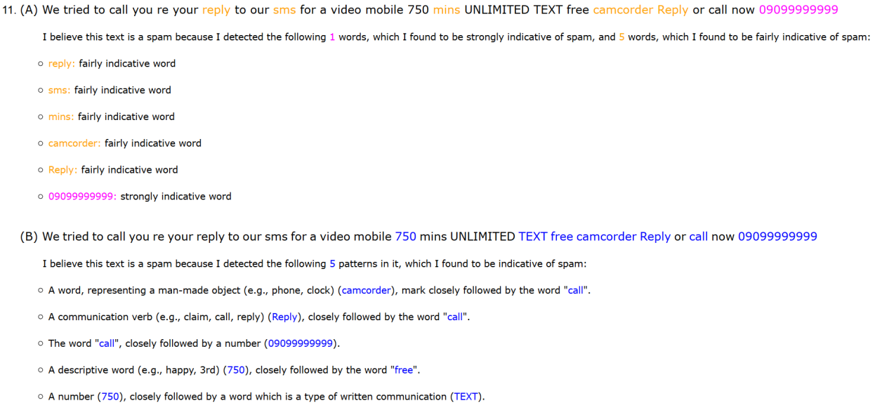
Figure 1: A screenshot of one of the sentences presented in the user study. In this sample grasp was randomly selected to appear second (B).

Table 5: Results and grasp-lite configuration of all experiments, ordered by F1 per dataset-category

dataset-category	method	P%	R%	F${}_{1}\%$	with surface form?	Fβ	top K patterns in use	min matches for positive
AG’s news business	LDA	27	35	31
	NB	25	76	37
	GrASP${}^{\hskip 1.0pt{\textrm{{lite}}}}$+GE	26	96	41	N	0.5	100	5
	prior	26	100	41
	GrASP${}^{\hskip 1.0pt{\textrm{{lite}}}}$+Split	65	71	68	Y	0.1	100	1
	NB on dev	67	74	70
	SIB	83	77	80
AG’s news sci/tech	LDA	27	22	24
	NB	23	71	34
	GrASP${}^{\hskip 1.0pt{\textrm{{lite}}}}$+GE	23	88	36	N	0.5	25	1
	prior	30	100	46
	NB on dev	72	70	71
	GrASP${}^{\hskip 1.0pt{\textrm{{lite}}}}$+Split	70	78	74	Y	0.05	100	1
	SIB	81	82	81
AG’s news sports	LDA	25	32	28
	NB	26	80	39
	prior	25	100	40
	GrASP${}^{\hskip 1.0pt{\textrm{{lite}}}}$+GE	51	62	56	N	0.5	10	5
	GrASP${}^{\hskip 1.0pt{\textrm{{lite}}}}$+GE	51	62	56	Y	0.5	10	5
	GrASP${}^{\hskip 1.0pt{\textrm{{lite}}}}$+Split	82	80	81	Y	0.05	100	1
	NB on dev	86	81	84
	SIB	93	94	94
AG’s news world	LDA	24	32	27
	prior	25	100	40
	NB	27	85	41
	GrASP${}^{\hskip 1.0pt{\textrm{{lite}}}}$+GE	31	84	46	Y	0.5	10	2
	GrASP${}^{\hskip 1.0pt{\textrm{{lite}}}}$+Split	75	77	76	Y	0.05	100	1
	NB on dev	79	77	78
	SIB	84	88	86
ASRD argument	BlendNet	52	32	40
	SIB	35	58	44
	NB on dev	35	65	46
	LDA	40	56	46
	prior	36	100	53
	NB	38	96	54
	GrASP${}^{\hskip 1.0pt{\textrm{{lite}}}}$+Split	40	85	55	N	1	50	1
	GrASP${}^{\hskip 1.0pt{\textrm{{lite}}}}$+GE	40	94	56	Y	0.05	100	1
	BERT	46	76	57
Essays claim	LDA	18	31	23
	BERT	27	25	26
	SIB	23	38	29
	NB on dev	18	79	30
	BlendNet	28	36	31
	GrASP${}^{\hskip 1.0pt{\textrm{{lite}}}}$+Split	19	96	32	Y	0.5	50	5
	GrASP${}^{\hskip 1.0pt{\textrm{{lite}}}}$+Split	19	96	32	N	0.5	100	10
	prior	19	100	32
	NB	21	72	33
	GrASP${}^{\hskip 1.0pt{\textrm{{lite}}}}$+GE	23	60	33	N	0.5	10	2
Essays major claim	LDA	7	21	11
	NB on dev	9	79	16
	BlendNet	12	32	17
	prior	9	100	17
	SIB	12	42	19
	NB	12	81	20
	GrASP${}^{\hskip 1.0pt{\textrm{{lite}}}}$+Split	12	74	21	N	1	10	5
	BERT	46	34	39
	GrASP${}^{\hskip 1.0pt{\textrm{{lite}}}}$+GE	32	65	42	Y	0.1	10	1
Essays premise	BlendNet	43	18	26
	LDA	55	42	48
	NB	67	46	54
	SIB	61	49	55
	NB on dev	57	82	68
	GrASP${}^{\hskip 1.0pt{\textrm{{lite}}}}$+GE	56	90	69	N	0.5	25	1
	GrASP${}^{\hskip 1.0pt{\textrm{{lite}}}}$+Split	56	95	71	Y	0.5	10	2
	prior	56	100	72
	BERT	69	86	76
HOLJ background	LDA	43	15	22
	SIB	59	22	32
	NB	40	93	56
	prior	41	100	58
	NB on dev	46	81	59
	GrASP${}^{\hskip 1.0pt{\textrm{{lite}}}}$+Split	57	76	65	Y	0.5	10	1
	GrASP${}^{\hskip 1.0pt{\textrm{{lite}}}}$+GE	75	61	67	Y	0.1	50	2
	GrASP${}^{\hskip 1.0pt{\textrm{{lite}}}}$+GE	75	61	67	Y	0.05	50	2
	BERT	73	67	70
HOLJ disposal	LDA	7	14	9
	prior	7	100	13
	NB	7	97	13
	NB on dev	11	24	15
	SIB	13	27	17
	GrASP${}^{\hskip 1.0pt{\textrm{{lite}}}}$+GE	26	43	32	Y	0.5	10	2
	GrASP${}^{\hskip 1.0pt{\textrm{{lite}}}}$+Split	41	43	42	N	1	10	5
	BERT	59	51	55
HOLJ fact	SIB	9	13	11
	GrASP${}^{\hskip 1.0pt{\textrm{{lite}}}}$+GE	8	46	13	N	0.5	100	1
	NB on dev	8	63	15
	NB	9	88	16
	prior	10	100	18
	LDA	14	25	18
	GrASP${}^{\hskip 1.0pt{\textrm{{lite}}}}$+Split	15	62	25	Y	1	10	5
	BERT	62	51	56
HOLJ framing	LDA	22	18	20
	GrASP${}^{\hskip 1.0pt{\textrm{{lite}}}}$+GE	15	66	24	Y	0.5	100	1
	SIB	27	24	25
	NB on dev	19	76	30
	NB	18	97	31
	prior	18	100	31
	GrASP${}^{\hskip 1.0pt{\textrm{{lite}}}}$+Split	30	78	43	N	0.5	100	10
	BERT	49	65	55
HOLJ proceedings	LDA	19	14	16
	SIB	20	16	18
	NB	18	92	30
	prior	17	100	30
	GrASP${}^{\hskip 1.0pt{\textrm{{lite}}}}$+Split	21	76	33	Y	0.5	25	1
	GrASP${}^{\hskip 1.0pt{\textrm{{lite}}}}$+GE	38	37	38	N	0.1	10	1
	NB on dev	43	36	39
	BERT	44	50	47
HOLJ textual	SIB	9	18	12
	prior	7	100	13
	NB	7	95	14
	NB on dev	7	74	14
	LDA	11	21	14
	GrASP${}^{\hskip 1.0pt{\textrm{{lite}}}}$+Split	13	28	18	N	0.05	25	1
	GrASP${}^{\hskip 1.0pt{\textrm{{lite}}}}$+GE	14	44	21	Y	0.5	10	1
	BERT	75	51	60
ISEAR anger	LDA	15	16	16
	NB	14	78	24
	prior	14	100	24
	SIB	19	35	25
	NB on dev	26	26	26
	GrASP${}^{\hskip 1.0pt{\textrm{{lite}}}}$+Split	16	74	27	N	0.5	50	1
	GrASP${}^{\hskip 1.0pt{\textrm{{lite}}}}$+GE	21	39	27	N	0.05	10	1
ISEAR disgust	LDA	13	15	14
	SIB	20	21	20
	GrASP${}^{\hskip 1.0pt{\textrm{{lite}}}}$+GE	15	77	24	Y	0.5	100	10
	NB on dev	65	16	25
	NB	16	79	27
	GrASP${}^{\hskip 1.0pt{\textrm{{lite}}}}$+Split	16	94	28	Y	1	100	10
	GrASP${}^{\hskip 1.0pt{\textrm{{lite}}}}$+Split	16	94	28	N	1	100	10
	prior	16	100	28
ISEAR fear	LDA	14	14	14
	NB	14	76	24
	prior	15	100	26
	GrASP${}^{\hskip 1.0pt{\textrm{{lite}}}}$+GE	18	67	28	Y	0.5	25	5
	NB on dev	33	68	44
	GrASP${}^{\hskip 1.0pt{\textrm{{lite}}}}$+Split	48	41	44	Y	0.05	25	1
	SIB	47	53	50
ISEAR guilt	LDA	17	21	19
	GrASP${}^{\hskip 1.0pt{\textrm{{lite}}}}$+GE	14	73	24	Y	0.05	100	5
	prior	14	100	25
	NB	15	86	26
	GrASP${}^{\hskip 1.0pt{\textrm{{lite}}}}$+Split	23	33	27	Y	0.5	10	1
	NB on dev	28	32	30
	SIB	28	50	36
ISEAR joy	LDA	14	17	15
	prior	13	100	23
	NB	19	32	24
	GrASP${}^{\hskip 1.0pt{\textrm{{lite}}}}$+GE	16	75	27	N	0.05	50	1
	GrASP${}^{\hskip 1.0pt{\textrm{{lite}}}}$+Split	36	38	37	Y	0.05	50	1
	SIB	43	43	43
	NB on dev	55	39	46
ISEAR sadness	LDA	17	19	18
	prior	15	100	25
	NB	15	83	26
	GrASP${}^{\hskip 1.0pt{\textrm{{lite}}}}$+GE	16	79	27	Y	0.5	50	5
	GrASP${}^{\hskip 1.0pt{\textrm{{lite}}}}$+Split	56	29	38	N	0.1	10	1
	NB on dev	45	38	41
	SIB	48	42	45
ISEAR shame	SIB	12	11	11
	LDA	11	13	12
	NB	14	80	23
	GrASP${}^{\hskip 1.0pt{\textrm{{lite}}}}$+Split	15	62	24	Y	0.5	50	1
	prior	14	100	24
	GrASP${}^{\hskip 1.0pt{\textrm{{lite}}}}$+GE	16	71	27	N	0.05	50	1
	NB on dev	35	35	35
Polarity positive	LDA	50	55	52
	SIB	62	49	55
	NB on dev	56	59	58
	NB	50	89	64
	GrASP${}^{\hskip 1.0pt{\textrm{{lite}}}}$+Split	50	95	66	Y	1	50	10
	GrASP${}^{\hskip 1.0pt{\textrm{{lite}}}}$+GE	50	95	66	Y	0.5	50	1
	prior	50	100	66
	BERT	88	87	87
SMS spam	LDA	12	41	18
	prior	13	100	23
	NB	18	93	30
	SIB	34	98	50
	GrASP${}^{\hskip 1.0pt{\textrm{{lite}}}}$+GE	51	79	62	N	0.1	10	1
	GrASP${}^{\hskip 1.0pt{\textrm{{lite}}}}$+Split	93	73	82	Y	0.05	100	5
	NB on dev	96	75	84
	BERT	97	97	97
Subjectivity subjective	LDA	52	57	54
	prior	52	100	68
	NB	58	87	69
	GrASP${}^{\hskip 1.0pt{\textrm{{lite}}}}$+GE	55	94	70	N	0.5	50	2
	NB on dev	67	84	74
	GrASP${}^{\hskip 1.0pt{\textrm{{lite}}}}$+Split	79	79	79	Y	0.05	100	1
	SIB	89	93	91
	BERT	98	96	97
ToS unfair clause	BERT	0	0	0
	LDA	11	51	18
	SIB	12	53	19
	NB on dev	11	100	20
	prior	11	100	20
	NB	11	100	20
	GrASP${}^{\hskip 1.0pt{\textrm{{lite}}}}$+Split	18	43	25	N	0.5	10	5
	GrASP${}^{\hskip 1.0pt{\textrm{{lite}}}}$+GE	25	42	32	Y	0.1	25	5
Wiki attack	NB on dev	11	96	20
	prior	12	100	21
	LDA	12	83	21
	NB	13	95	22
	SIB	24	89	38
	BERT	86	74	80
	GrASP${}^{\hskip 1.0pt{\textrm{{lite}}}}$+GE	12	93	21	Y	0.5	50	1
	GrASP${}^{\hskip 1.0pt{\textrm{{lite}}}}$+Split	54	38	44	Y	0.05	10	1

References

- Aharoni et al. (2014) Ehud Aharoni, Anatoly Polnarov, Tamar Lavee, Daniel Hershcovich, Ran Levy, Ruty Rinott, Dan Gutfreund, and Noam Slonim. 2014. A benchmark dataset for automatic detection of claims and evidence in the context of controversial topics. In Proceedings of the first Workshop on Argumentation Mining, pages 64–68.
- Almeida et al. (2011) Tiago A. Almeida, José María Gómez Hidalgo, and Akebo Yamakami. 2011. Contributions to the study of sms spam filtering: new collection and results. In ACM Symposium on Document Engineering, pages 259–262. ACM.
- Arrieta et al. (2019) Alejandro Barredo Arrieta, Natalia Díaz-Rodríguez, Javier Del Ser, Adrien Bennetot, Siham Tabik, Alberto Barbado, Salvador García, Sergio Gil-López, Daniel Molina, Richard Benjamins, Raja Chatila, and Francisco Herrera. 2019. Explainable artificial intelligence (xai): Concepts, taxonomies, opportunities and challenges toward responsible ai.
- Blei et al. (2003) David M. Blei, Andrew Y. Ng, and Michael I. Jordan. 2003. Latent dirichlet allocation. Journal of Machine Learning Research, 3:2003.
- Brandes and Dover (2018) Leif Brandes and Yaniv Dover. 2018. Post-consumption susceptibility of online reviewers to random weather-related events. PloS ONE.
- Choshen and Abend (2018) Leshem Choshen and Omri Abend. 2018. Inherent biases in reference-based evaluation for grammatical error correction. In Proceedings of the 56th Annual Meeting of the Association for Computational Linguistics (Volume 1: Long Papers), pages 632–642, Melbourne, Australia. Association for Computational Linguistics.
- Choshen-Hillel et al. (2019) Shoham Choshen-Hillel, Alex Shaw, and Eugene M. Caruso. 2019. Lying to appear honest. Journal of Experimental Psychology: General. Conditionally accepted.
- Cohen (1960) Cohen. 1960. A coefficient of agreement for nominal scales. Educ Psychol Meas, pages 37–46.
- Devlin et al. (2019) Jacob Devlin, Ming-Wei Chang, Kenton Lee, and Kristina Toutanova. 2019. Bert: Pre-training of deep bidirectional transformers for language understanding. In NAACL-HLT.
- Dodge et al. (2020) Jesse Dodge, Gabriel Ilharco, Roy Schwartz, Ali Farhadi, Hannaneh Hajishirzi, and Noah A. Smith. 2020. Fine-tuning pretrained language models: Weight initializations, data orders, and early stopping. ArXiv, abs/2002.06305.
- Dorr (1994) Bonnie J. Dorr. 1994. Machine translation divergences: A formal description and proposed solution. Computational Linguistics, 20(4):597–633.
- Ein-Dor et al. (2019) Liat Ein-Dor, Eyal Shnarch, Lena Dankin, Alon Halfon, Benjamin Sznajder, Ariel Gera, Carlos Alzate, Martin Gleize, Leshem Choshen, Yufang Hou, et al. 2019. Corpus wide argument mining–a working solution. arXiv preprint arXiv:1911.10763.
- Fekete and Primet (2016) Jean-Daniel Fekete and Romain Primet. 2016. Progressive analytics: A computation paradigm for exploratory data analysis. arXiv preprint arXiv:1607.05162.
- Ghaeini et al. (2018) Reza Ghaeini, Xiaoli Fern, and Prasad Tadepalli. 2018. Interpreting recurrent and attention-based neural models: a case study on natural language inference. In Proceedings of the 2018 Conference on Empirical Methods in Natural Language Processing, pages 4952–4957, Brussels, Belgium. Association for Computational Linguistics.
- Gilpin et al. (2018) Leilani H. Gilpin, David Bau, Ben Z. Yuan, Ayesha Bajwa, Michael Specter, and Lalana Kagal. 2018. Explaining explanations: An overview of interpretability of machine learning.
- Grover et al. (2004) Claire Grover, Ben Hachey, and Ian Hughson. 2004. The HOLJ corpus: Supporting summarisation of legal texts. In Proceedings of the 5th International Workshop on Linguistically Interpreted Corpora, pages 47–54.
- Grundkiewicz and Junczys-Dowmunt (2014) Roman Grundkiewicz and Marcin Junczys-Dowmunt. 2014. The wiked error corpus: A corpus of corrective wikipedia edits and its application to grammatical error correction. In International Conference on Natural Language Processing, pages 478–490. Springer.
- Hearst (1992) Marti A. Hearst. 1992. Automatic acquisition of hyponyms from large text corpora. In COLING 1992 Volume 2: The 15th International Conference on Computational Linguistics.
- Hu and Liu (2004) Minqing Hu and Bing Liu. 2004. Mining and summarizing customer reviews. In International Conference on Knowledge Discovery and Data Mining, KDD ’04, pages 168–177.
- Koehn et al. (2019) Philipp Koehn, Francisco Guzmán, Vishrav Chaudhary, and Juan Pino. 2019. Findings of the WMT 2019 shared task on parallel corpus filtering for low-resource conditions. In Proceedings of the Fourth Conference on Machine Translation (Volume 3: Shared Task Papers, Day 2), pages 54–72.
- Koptient et al. (2019) Anaïs Koptient, Rémi Cardon, and Natalia Grabar. 2019. Simplification-induced transformations: typology and some characteristics. In Proceedings of the 18th BioNLP Workshop and Shared Task, pages 309–318, Florence, Italy. Association for Computational Linguistics.
- Kukich (1992) Karen Kukich. 1992. Techniques for automatically correcting words in text. ACM Comput. Surv., 24(4):377–439.
- Lertvittayakumjorn and Toni (2019) Piyawat Lertvittayakumjorn and Francesca Toni. 2019. Human-grounded evaluations of explanation methods for text classification. In Proceedings of the 2019 Conference on Empirical Methods in Natural Language Processing and the 9th International Joint Conference on Natural Language Processing (EMNLP-IJCNLP), pages 5195–5205, Hong Kong, China. Association for Computational Linguistics.
- Li et al. (2019) Bowei Li, Yongzheng Zhang, Junliang Yao, and Tao Yin. 2019. Mdba: Detecting malware based on bytes n-gram with association mining. 2019 26th International Conference on Telecommunications (ICT), pages 227–232.
- Lippi et al. (2019) Marco Lippi, Przemyslaw Palka, Giuseppe Contissa, Francesca Lagioia, Hans-Wolfgang Micklitz, Giovanni Sartor, and Paolo Torroni. 2019. Claudette: an automated detector of potentially unfair clauses in online terms of service. Artificial Intelligence and Law, 27:117–139.
- Miller (1998) George Miller. 1998. WordNet: An electronic lexical database. MIT press.
- Mirkin et al. (2018a) Shachar Mirkin, Michal Jacovi, Tamar Lavee, Hong-Kwang Kuo, Samuel Thomas, Leslie Sager, Lili Kotlerman, Elad Venezian, and Noam Slonim. 2018a. A recorded debating dataset. In Proceedings of the Eleventh International Conference on Language Resources and Evaluation (LREC 2018), Miyazaki, Japan. European Language Resources Association (ELRA).
- Mirkin et al. (2018b) Shachar Mirkin, Guy Moshkowich, Matan Orbach, Lili Kotlerman, Yoav Kantor, Tamar Lavee, Michal Jacovi, Yonatan Bilu, Ranit Aharonov, and Noam Slonim. 2018b. Listening comprehension over argumentative content. In Proceedings of the 2018 Conference on Empirical Methods in Natural Language Processing, pages 719–724, Brussels, Belgium. Association for Computational Linguistics.
- Nguyen et al. (2010) Anthony N. Nguyen, Michael Lawley, David P. Hansen, Rayleen V. Bowman, Belinda E. Clarke, Edwina E. Duhig, and Shoni Colquist. 2010. Symbolic rule-based classification of lung cancer stages from free-text pathology reports. Journal of the American Medical Informatics Association : JAMIA, 17 4:440–5.
- Nidhi and Singh (2018) Ritu Nidhi and Tanya Singh. 2018. English-maithili machine translation and divergence. In 2018 7th International Conference on Reliability, Infocom Technologies and Optimization (Trends and Future Directions)(ICRITO), pages 775–778. IEEE.
- Padillo et al. (2019) Francisco Padillo, José María Luna, and Sebastián Ventura. 2019. Evaluating associative classification algorithms for big data. Big Data Analytics, 4:1–27.
- Pang and Lee (2004) Bo Pang and Lillian Lee. 2004. A sentimental education: Sentiment analysis using subjectivity summarization based on minimum cuts. In Proceedings of the 42nd Annual Meeting of the Association for Computational Linguistics (ACL-04), pages 271–278, Barcelona, Spain.
- Pang and Lee (2005) Bo Pang and Lillian Lee. 2005. Seeing stars: Exploiting class relationships for sentiment categorization with respect to rating scales. In Proceedings of the 43rd Annual Meeting of the Association for Computational Linguistics (ACL’05), pages 115–124, Ann Arbor, Michigan. Association for Computational Linguistics.
- Ravichandran and Hovy (2002) Deepak Ravichandran and Eduard Hovy. 2002. Learning surface text patterns for a question answering system. In Proceedings of the 40th Annual Meeting of the Association for Computational Linguistics, pages 41–47, Philadelphia, Pennsylvania, USA. Association for Computational Linguistics.
- Ribeiro et al. (2016) Marco Tulio Ribeiro, Sameer Singh, and Carlos Guestrin. 2016. Why should i trust you?“: Explaining the predictions of any classifier. In Proceedings of the 22Nd ACM SIGKDD International Conference on Knowledge Discovery and Data Mining (New York, NY, USA, 2016), page 1135–1144.
- Rinott et al. (2015) Ruty Rinott, Lena Dankin, Carlos Alzate Perez, Mitesh M. Khapra, Ehud Aharoni, and Noam Slonim. 2015. Show me your evidence - an automatic method for context dependent evidence detection. In emnlp-15, pages 440–450.
- Schwartz (2017) Roy Schwartz. 2017. Pattern-based methods for Improved Lexical Semantics and Word Embeddings. Ph.D. thesis, Hebrew University of Jerusalem.
- Shao et al. (2015) Bo Shao, Lorna Doucet, and David R. Caruso. 2015. Universality versus cultural specificity of three emotion domains: Some evidence based on the cascading model of emotional intelligence. Journal of Cross-Cultural Psychology, 46(2):229–251.
- Shnarch et al. (2018) Eyal Shnarch, Carlos Alzate, Lena Dankin, Martin Gleize, Yufang Hou, Leshem Choshen, Ranit Aharonov, and Noam Slonim. 2018. Will it blend? blending weak and strong labeled data in a neural network for argumentation mining. In Proceedings of ACL, pages 599–605. Association for Computational Linguistics.
- Shnarch et al. (2017) Eyal Shnarch, Ran Levy, Vikas Raykar, and Noam Slonim. 2017. GRASP: Rich patterns for argumentation mining. In Proceedings of the 2017 Conference on Empirical Methods in Natural Language Processing, Copenhagen, Denmark. Association for Computational Linguistics.
- Slonim et al. (2013) Noam Slonim, Ehud Aharoni, and Koby Crammer. 2013. Hartigan’s k-means versus lloyd’s k-means: is it time for a change? In Proceedings of the 23rd International Joint Conference on Artificial Intelligence, pages 1677–1684.
- Slonim et al. (2002) Noam Slonim, Nir Friedman, and Naftali Tishby. 2002. Unsupervised document classification using sequential information maximization. In Proceedings of the 25th Annual International ACM SIGIR Conference on Research and Development in Information Retrieval, SIGIR ’02, page 129–136.
- Stab and Gurevych (2017) Christian Stab and Iryna Gurevych. 2017. Parsing argumentation structures in persuasive essays. Computational Linguistics, 43(3):619–659.
- Sydorova et al. (2019) Alona Sydorova, Nina Poerner, and Benjamin Roth. 2019. Interpretable question answering on knowledge bases and text. In Proceedings of the 57th Annual Meeting of the Association for Computational Linguistics, pages 4943–4951, Florence, Italy. Association for Computational Linguistics.
- Wulczyn et al. (2017) Ellery Wulczyn, Nithum Thain, and Lucas Dixon. 2017. Wikipedia Talk Labels: Personal Attacks. Kaggle.
- Yu (1977) Chong Ho Yu. 1977. Exploratory data analysis. Methods, 2:131–160.
- Zhang et al. (2015) Xiang Zhang, Junbo Zhao, and Yann LeCun. 2015. Character-level convolutional networks for text classification. In Advances in neural information processing systems, pages 649–657.
- Ziser and Reichart (2018) Yftah Ziser and Roi Reichart. 2018. Pivot based language modeling for improved neural domain adaptation. In Proceedings of the 2018 Conference of the North American Chapter of the Association for Computational Linguistics: Human Language Technologies, Volume 1 (Long Papers), pages 1241–1251, New Orleans, Louisiana. Association for Computational Linguistics.