Velocity derivatives in a high Reynolds number turbulent boundary layer. Part III: Optimization of an SPIV experiment for derivative moments assessment

Abstract

An SPIV experiment using two orthogonal planes simultaneously was performed in the LML boundary layer facility to specifically measure all of the derivative moments needed to estimate the dissipation rate of the Turbulence Kinetic Energy. The Reynolds number was $Re_{\theta}=7500$ or $Re_{\tau}=2300$. A detailed analysis of the errors in derivative measurements was carried out, as well as applying and using consistency checks derived from the continuity equation. The random noise error was quantified, and used to “de-noise” the derivative moments. A comparison with a DNS channel flow at comparable Reynolds number demonstrated the capability of the technique. The results were further validated using the recent theory developed by George and Stanislas (2020). The resulting data have been extensively used in parts I and II of the present contribution to study near wall dissipation (Stanislas et al. (2020); George et al. (2020)). An important result of the present work is the provision of reliable rules for an accurate assessment of the dissipation in future PIV experiments.

¹ Univ. Lille, CNRS, ONERA, Arts et Metiers Institute of Technology, Centrale Lille, UMR 9014 - LMFL - Laboratoire de Mécanique des Fluides de Lille - Kampé de Fériet, F-59000 Lille, France
² Visiting Pr., Centrale Lille, F59651 Villeneuve d’Ascq, France
³ Pr. Emeritus, Centrale Lille, F59651 Villeneuve d’Ascq, France

Received: date / Accepted: date

1 Introduction

Most experiments in wall turbulence using PIV seek understanding of the flow organization. This objective generally involves also gathering information from the velocity fields. The basic statistics extracted from the velocity (mean and RMS velocities, Reynolds stresses…) are of prime interest when looking at the momentum equation, but they do not provide much information as soon as the energy transfer is of interest. For this, derivatives of the velocity fields have to be computed to access parameters based on velocity gradients such as the rate-of-strain tensor and its invariants, vorticity or the dissipation rate of Turbulence Kinetic Energy (both as a tensor in the Reynolds stress transport equation or as a scalar in the Turbulence Kinetic Energy equation). The dissipation rate, say $\varepsilon$, is a key parameter of the turbulence and it needs to be modeled to properly represent turbulence with the RANS equations. It is also a key to understanding the behaviour of the smallest scales of turbulence. In part I (Stanislas et al. (2020)) and part II (George et al. (2020)) of this contribution, the results of an SPIV experiment were analysed in detail together with those of a DNS at comparable Reynolds number to obtain a better understanding of the turbulence dissipation. In the present paper, attention will be focussed on the experimental approach used to measure the fluctuating velocity gradients and to obtain the results discussed in those two previous papers.

1.1 The basic equations

All the relevant turbulence equations are presented and discussed in detail in parts I and II, so only the most essential will be repeated here. Most important, of course, is the scalar dissipation rate which appears in the transport equation for the Turbulence Kinetic Energy given by:

$$\varepsilon=\nu\left[\left\langle\frac{\partial u_{i}}{\partial x_{j}}\frac{\partial u_{i}}{\partial x_{j}}\right\rangle+\left\langle\frac{\partial u_{i}}{\partial x_{j}}\frac{\partial u_{j}}{\partial x_{i}}\right\rangle\right]$$ (1)

This is of course just twice the viscosity times the mean square fluctuating strain rate, $\varepsilon=2\nu\langle s_{ij}s_{ij}\rangle$. To compute this full dissipation it is necessary to measure all the components of the instantaneous gradient tensor and to compute the variance of each term together with a few covariances. This corresponds to a total of twelve terms which can be organized in three groups:

$$\varepsilon = \nu\left\{2\left[\left\langle\frac{\partial u_{1}}{\partial x_{1}}\frac{\partial u_{1}}{\partial x_{1}}\right\rangle+\left\langle\frac{\partial u_{2}}{\partial x_{2}}\frac{\partial u_{2}}{\partial x_{2}}\right\rangle+\left\langle\frac{\partial u_{3}}{\partial x_{3}}\frac{\partial u_{3}}{\partial x_{3}}\right\rangle\right]\right.$$ (2)

$$+ \left[\left\langle\frac{\partial u_{1}}{\partial x_{2}}\frac{\partial u_{1}}{\partial x_{2}}\right\rangle+\left\langle\frac{\partial u_{2}}{\partial x_{1}}\frac{\partial u_{2}}{\partial x_{1}}\right\rangle+\left\langle\frac{\partial u_{1}}{\partial x_{3}}\frac{\partial u_{1}}{\partial x_{3}}\right\rangle\right.\hskip 45.5244pt$$

$$+ \left.\left\langle\frac{\partial u_{3}}{\partial x_{1}}\frac{\partial u_{3}}{\partial x_{1}}\right\rangle+\left\langle\frac{\partial u_{2}}{\partial x_{3}}\frac{\partial u_{2}}{\partial x_{3}}\right\rangle+\left\langle\frac{\partial u_{3}}{\partial x_{2}}\frac{\partial u_{3}}{\partial x_{2}}\right\rangle\right]$$

$$+ 2\left[\left\langle\frac{\partial u_{1}}{\partial x_{2}}\frac{\partial u_{2}}{\partial x_{1}}\right\rangle+\left\langle\frac{\partial u_{1}}{\partial x_{3}}\frac{\partial u_{3}}{\partial x_{1}}+\left\langle\frac{\partial u_{1}}{\partial x_{3}}\frac{\partial u_{3}}{\partial x_{1}}\right\rangle\right]\right\}$$

All of these are difficult to measure accurately. The dissipation rate $\varepsilon$ as given by equation (1) combines both derivatives and statistical computations. The tensorial counterpart of the dissipation, say $\varepsilon_{ik}$, is even more complicated and is included in Part II. Because of these difficulties, the turbulence community over the past 90 years has made several different hypotheses to simplify these measurements. Three of these hypotheses “local isotropy”, “local axisymmetry” and “local homogeneity”) were examined in detail in part II of this contribution (George et al. (2020)).

In the present contribution the objective is to review the methods used to determine the dissipation rate $\varepsilon$ of the TKE and all the components of the dissipation rate tensor $\varepsilon_{ij}$. And also to describe the dedicated Stereoscopic PIV experiment carried out in a turbulent boundary layer at high Reynolds number.

1.2 Brief review of SPIV

PIV is an imaging technique, based on a physical principle completely different from Hot Wire Anemometry (Heat transfer) or Laser Doppler Velocimetry (Doppler shift). It is very dependent on the characteristics of the CCD or CMOS sensor (which have made tremendous progress in the last twenty years) and on the properties of the laser light. It is well-known to evidence a high level of noise, which in turbulence is a problem at high spatial frequency where the signal is quite low. This is a real drawback when trying to measure velocity derivatives representative of the dissipative scales. Stereoscopic PIV is now an established method to characterize turbulent flow. It has been mostly used to look at the instantaneous structures in turbulence, but many researchers also use it to compute statistics such as mean velocity, Reynolds stress tensor, probability density function or spectra (Adrian et al. (2000); Foucaut et al. (2011); Herpin et al. (2012)). SPIV allows the measurement of the three components of the velocity in a plane with an accuracy at best of 1-2% (0.1 pixel) if the experiment is properly designed. For a turbulent flow, it opens the unique capability of studying the organization of the turbulence. Generally, due to the limited spatial resolution of PIV, the smallest scales of the flow cannot be investigated. One difficulty in the data processing comes from the noise amplification when derivatives have to be computed (Foucaut and Stanislas (2002)). However, the velocity gradients are necessary to determine the vorticity and shear. They are also essential for the detection of vortices when using the $Q$ criterion or the swirling strength, both useful tools to study the flow organization.

The possibilities of the SPIV technique can be significantly enlarged by the use of light polarization. Based on this laser light property, it is possible to record velocity fields in two crossed-planes simultaneously. When the planes are parallel, this method is called dual plane stereoscopic PIV  (Kahler and Stanislas (2000)). The dual plane technique allows the measurement of two velocity fields with an adjustable time delay or spatial separation between them. By varying this delay the space-time correlation of the velocity field can be computed. By varying the separation, the 3D spatial correlation can be obtained. Ganapathisubramani et al. (2005) used the dual plane technique to get the full gradient tensor and to study the near wall flow structures. If both planes are perpendicular instead of parallel, this can provide information about the spatial properties of the flow (e.g.,  Hambleton et al. (2006), Ganapathisubramani et al. (2006)) as a first step toward full 3D3C information as provided for example by TomoPIV or Holographic PIV.

1.3 The goals of this paper

In the present paper, Stereoscopic PIV in two crossing-planes is used to compute all the derivatives of the three velocity components in a turbulent boundary layer. The main limitation of PIV is that it only resolves a range of scales which is between the size of the field of view for the largest scales and that of the interrogation window for the smallest ones (c.f., Foucaut et al. (2004)). Due to these spatial resolution limits and to the PIV noise, access to the small scales relevant to dissipation is not an easy task. Emphasis is consequently put particularly here on the derivative filter choice and on the measurement noise management. The primary interest of the present approach is that everything possible was done to try to minimise the noise contribution, first on the velocity fields themselves, second on the derivatives and finally on the derivative moments which are necessary to access the dissipation rate of Turbulence Kinetic Energy (TKE). In the following these different steps will be detailed and, as much as possible quantified, with the aim of providing guidelines for future measurement of the dissipation with Stereoscopiv PIV. Finally the results will be compared to a recently developed theory by George and Stanislas (2020) predicting the PIV noise. These results provide a better understanding of the noise sources and how to minimize them.

2 Experimental setup

Various aspects of the experiment and methodology were of necessity included in Parts I and II. They will described in much more detail here to fill in the gaps for the experimentalists.

2.1 The wind-tunnel

Figure 1: Side view of the LMFL boundary layer wind tunnel

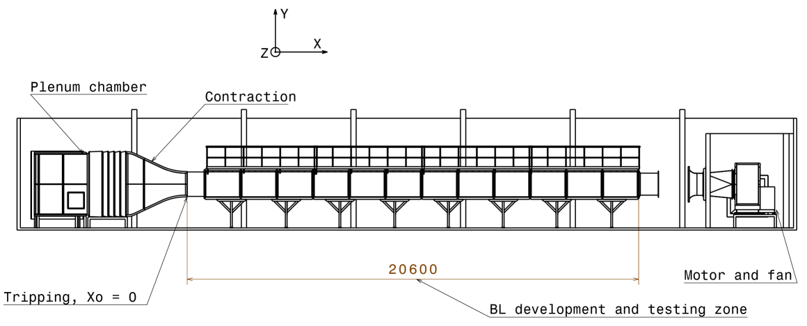
The experiment was carried out in the LMFL turbulent boundary layer wind tunnel sketched in figure 1. The test section is 1 m high, 2 m wide and 20 m long to allow the development of the boundary layer. The boundary layer thickness can reach 30 cm at the end of the test section. A slight favourable pressure gradient exist and has been characterized by Carlier and Stanislas (2005). It is of the order of 1 Pa/m. Two important characteristics of this wind tunnel are that first it is temperature-regulated at better than 0.5C, which allows accurate Hot Wire measurements with very long samples; second that it is fully transparent on 4 sides and down to the wall, which allows a lot of flexibility in the PIV and SPIV set-ups. The present experiment was carried out at a Reynolds number $R_{\theta}=7500$ ($Re_{\tau}=2300$) which corresponds to a free stream velocity of 3 m/s.

2.2 The optical setup, seeding and processing

Figure 2 shows a top-view of the SPIV set-up used for this experiment. The laser light sheets were generated with the help of a BMI YAG laser system specifically developed for LMFL. It is composed of 4 laser cavities which can deliver 200 mJ each. Two cavities are polarized vertically and two horizontally. Both sets of cavities are recombined two-by-two to provide two double pulse light beams orthogonally polarized. Lenses and mirrors generate light sheets slightly larger than the field of view to improve the uniformity of the illumination to introduce them in the wind tunnel. The tunnel walls are made of high quality glass, antireflection coated to minimize spurious light. The two light sheets were introduced through the ceiling of the tunnel and exited through the transparent floor where they where caught in a light trap.

Figure 2: Top view of the double SPIV experimental set-up

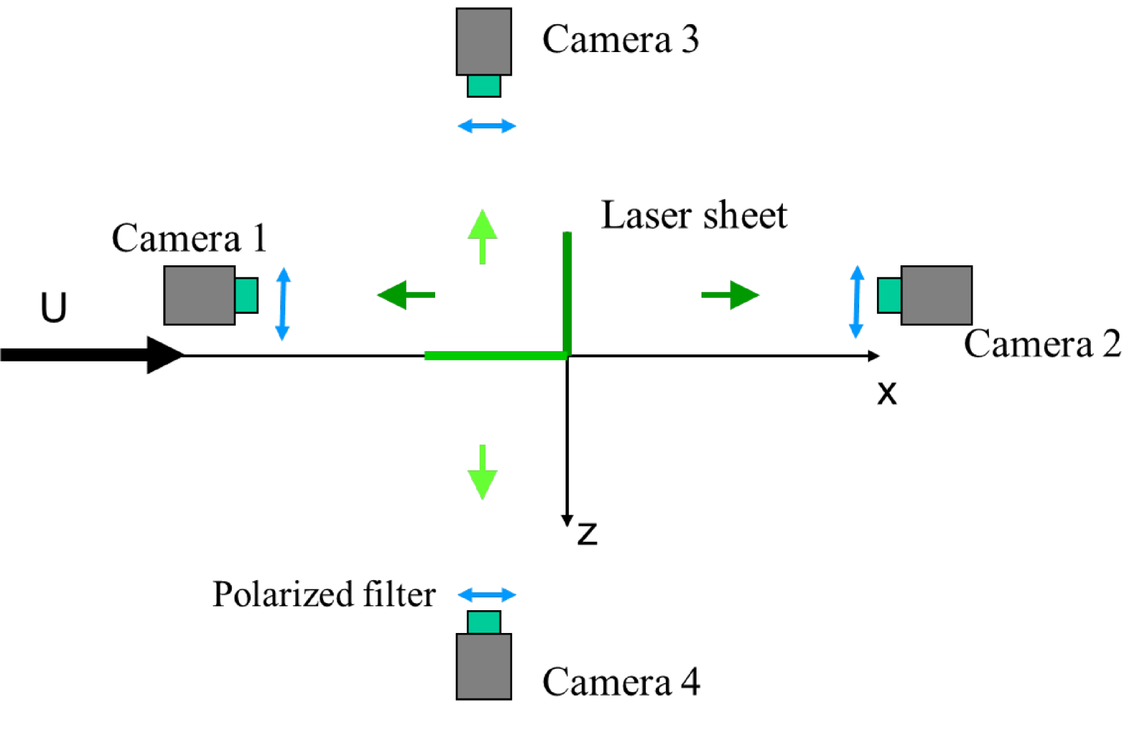
The field-of-view was imaged with two Stereoscopic PIV systems in two orthogonal crossing-planes, both normal to the wall. One plane was streamwise along ($x_{1},x_{2}$). The second one was spanwise along ($x_{3},x_{2}$), where $x_{2}$ is the wall normal coordinate. Each system was based on Hamamatsu 2k x 2k pixels cameras, micro Nikkor 105 mm lenses at f# 8 and polarizing filters. The field-of-view of each system is about 12 x 8 $cm^{2}$ (corresponding to about $640$ x $960$ wall units). Both systems were adjusted so that the two PIV planes share a common wall normal line. Each SPIV system was adjusted to fulfill the Scheimpflug conditions (Willert (1997)). The seeding was done with Poly-Ethylene Glycol micron particles. The particle size was of the order of 1 $\mu m$. In this configuration, the Airy disk diameter is of the order of 12.3 $\mu m$. On the Hamamtsu cameras, this gives a particle image size of the order of 1.8 pixel (c.f. Adrian (1997)). This was checked on the real images. On average, the particle image size appears to be effectively a bit less than 2 pixel. Following Raffel et al. (1998), such a size should minimize the peak-locking effect.

The images from both cameras were processed with a standard multi-grid and multi-pass algorithm with image deformation (Scarano (2002)). The analysis was made by the classical FFT-based cross-correlation method with symmetrical integer shift of both windows. Before the final fourth pass, image deformation was applied according to the displacements estimated from the three previous passes to improve the accuracy (Stanislas et al. (2007)). A 1-D Gaussian peak fitting algorithm was used for the sub-pixel displacement determination. The final interrogation window size was 24 x 32 pixels for each plane. It was chosen based on the HW turbulence spectrum in order to optimize the signal to noise ratio, following the method proposed by Foucaut et al. (2004). Such a size corresponds to a square window in the physical space of 1.4 x 1.4 $mm^{2}$ (11.6 x 11.6 wall units or 6 x 6 Kolmogorov units). An overlap of 66% was chosen in order to maximize the spatial resolution while bringing 34% of new information in each interrogation window.

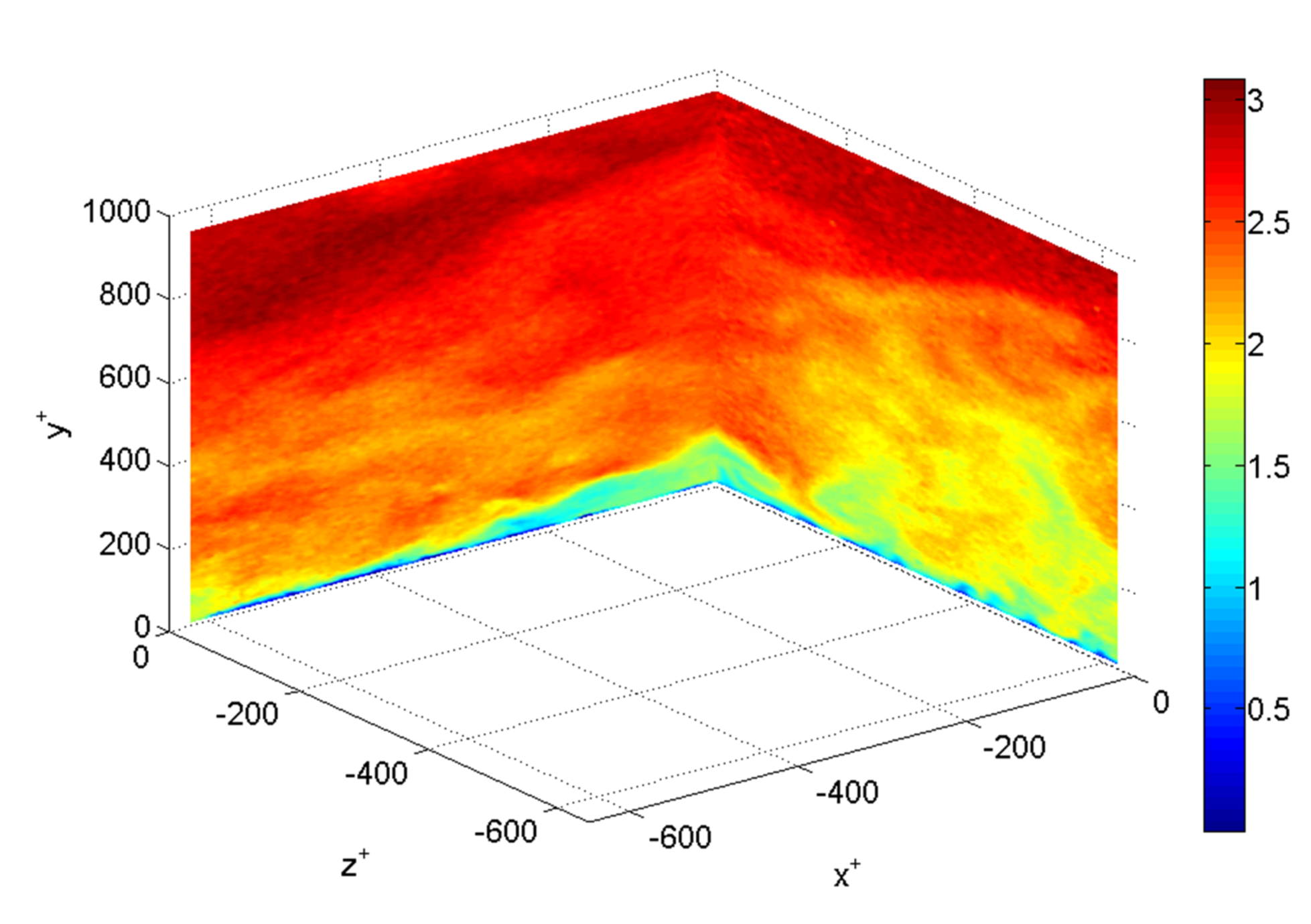
The Soloff method using 7 calibration planes was used to reconstruct the three velocity components in the plane of measurement (Soloff et al. (1997)). The calibration was done with different targets using crosses. From the set of recorded calibration planes and SPIV images, the misalignment between the light sheet and the calibration plane was corrected (Coudert and Schon (2001)) with a self-calibration method similar to the one proposed by Wieneke (2005). The analyses were performed using the MatPIV software adapted and extended by LMFL. A total of 12000 velocity fields were recorded simultaneously with the two systems and analysed. Figure 3 gives an example of the instantaneous streamwise velocity component $u_{1}$ in the two planes.

Figure 3: Example of instantaneous streamwise component velocity fields.

2.3 Basic flow characteristics

Figures 4 and 5 show the mean streamwise velocity and the turbulent intensity profiles from the two planes respectively, along with HWA results. All these results are in good agreement above 15 wall units, except for the spanwise intensity component in figure 5 which presents a difference below 40 wall units. This discrepancy is most probably due to the mean velocity gradient at the scale of the X-wire probe used, which cannot be taken into account during the calibration.

Figure 4: Mean velocity profiles from the two cross-planes compared to hot-wire data.

Figure 5: Turbulent intensity profiles from the two cross-planes compared to hot-wire data.

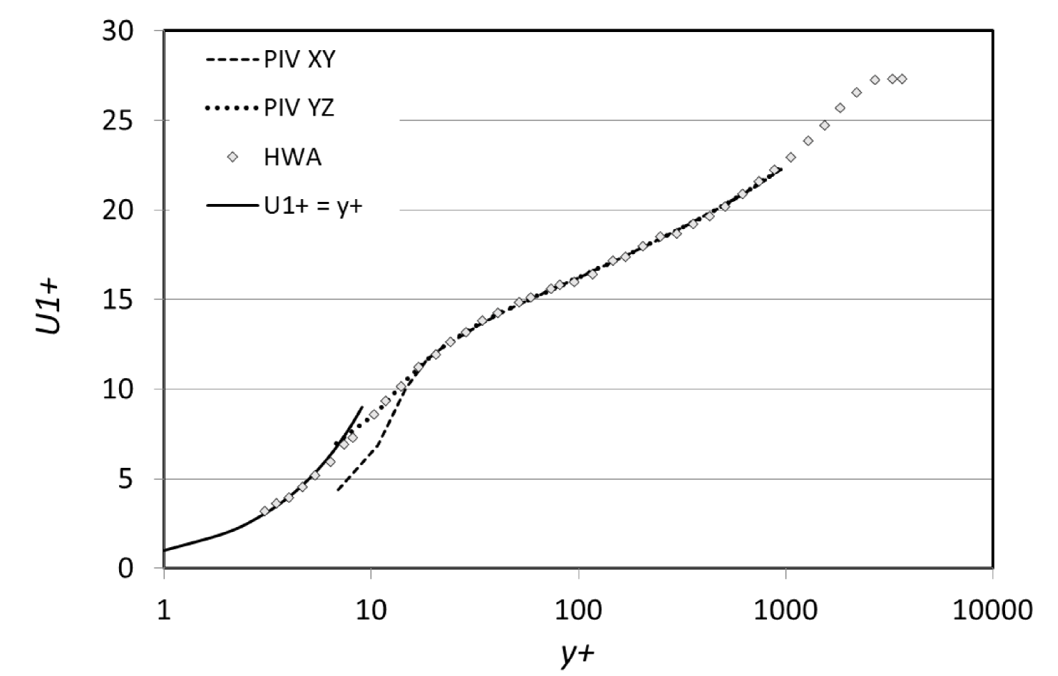
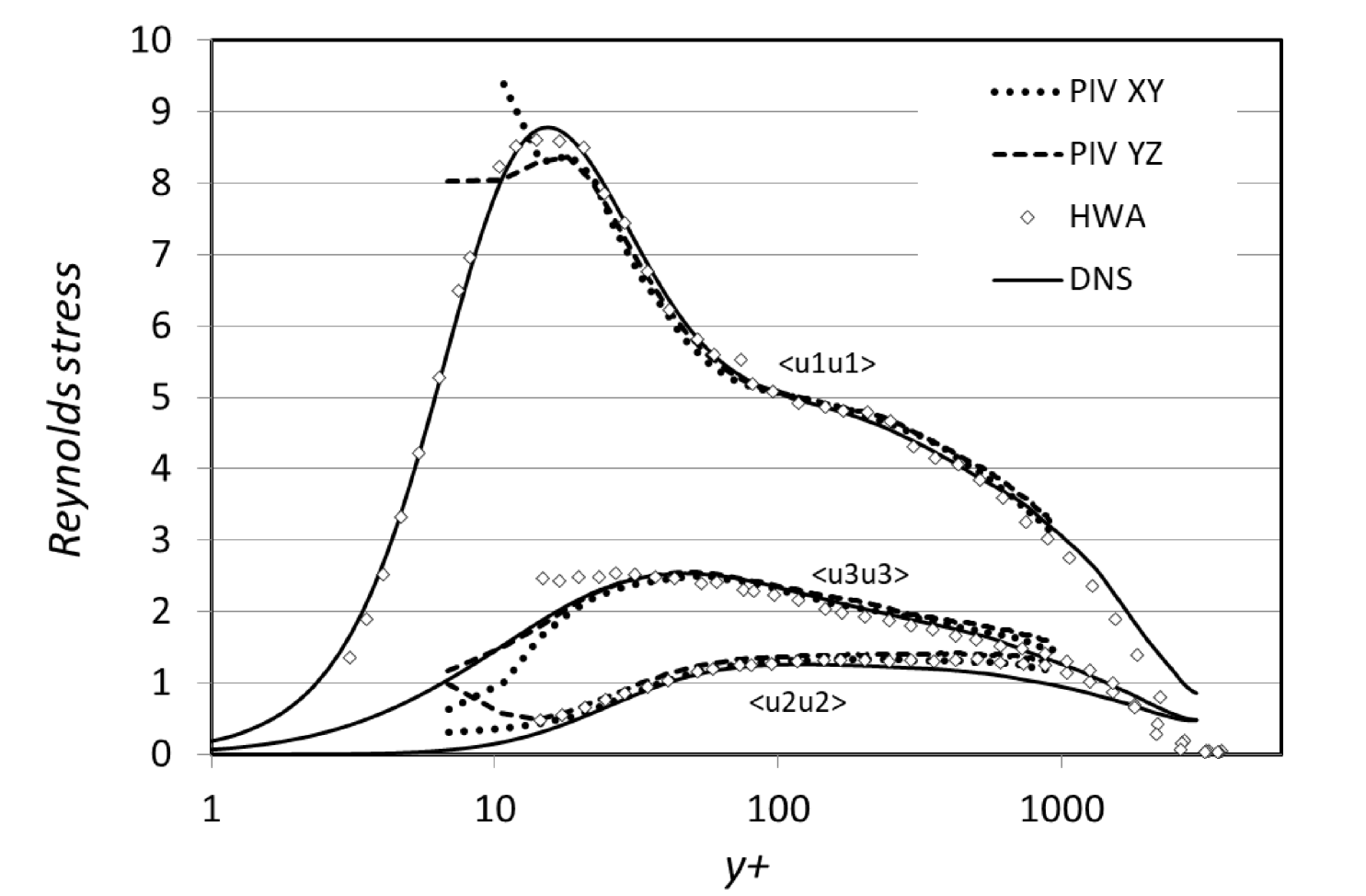
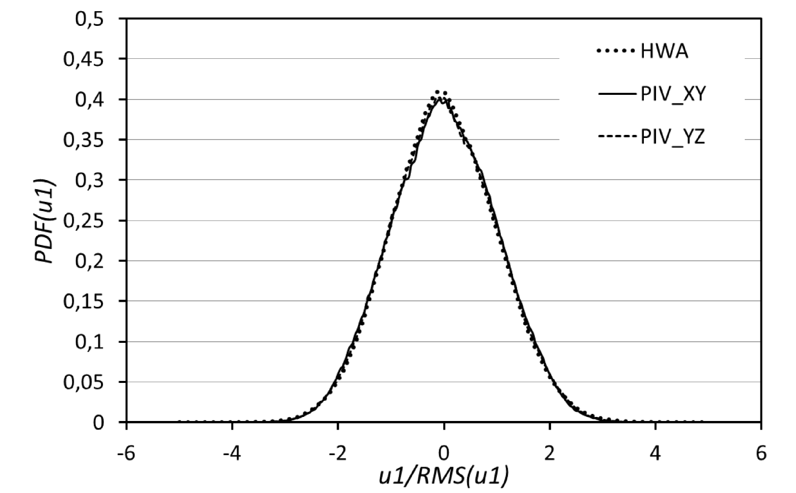
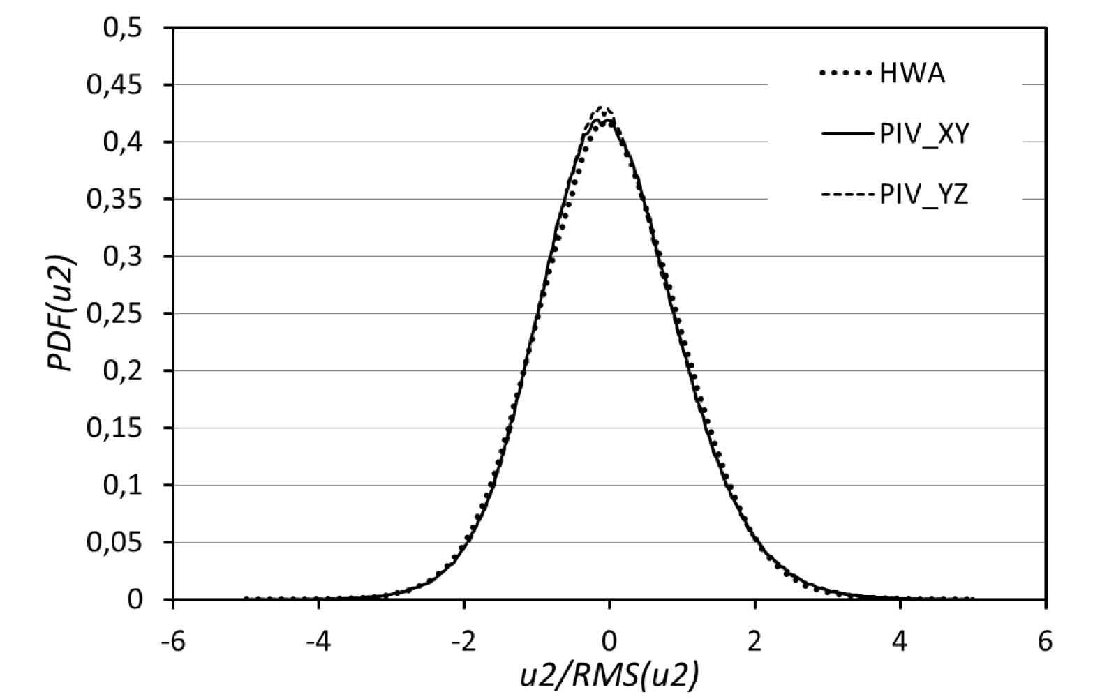
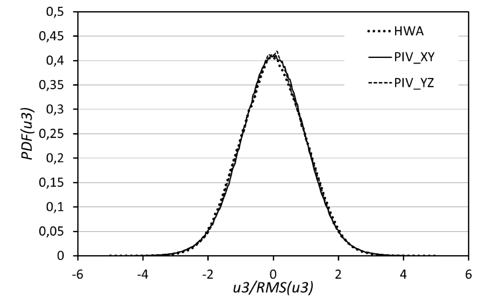
Figure 6 shows the probability density functions of the three fluctuating velocity components from both planes at 250 wall units and compared with hot wire anemometry. A very good agreement is observed between the two SPIV systems and the hot wire results. Also they show no clipping of the velocity due to a saturation of the dynamics in the plane normal to the flow and no peak locking is in evidence.

Figure 6: Comparison of the PDF of the 3 fluctuating velocity components from SPIV and HWA at $y^{+}=100$.

3 Velocity spectra and noise

Looking now at the spectrum, two important characteristics of the PIV technique have to be looked at: the limited field of view and the fact that an interrogation window of finite size is used. The influence of the IW size will be characterized in the next section when looking at the small scales.

3.1 The turbulence spectra

Note that here the spectra are being computed using spatial transforms of the entire field-of-view, and not by applying Taylor’s hypothesis to a time-varying signal at one location. The finite field-of-view multiplies the turbulent velocity field by a rectangular window which cuts off the large scales and generates leakage down the spectrum toward the small scales. In Fourier spectral space this manifests itself as a “sinc-squared”-function convolved with the spectrum.

Figure 7: Simulation of the influence of the limited field of view of PIV on the turbulence spectrum.

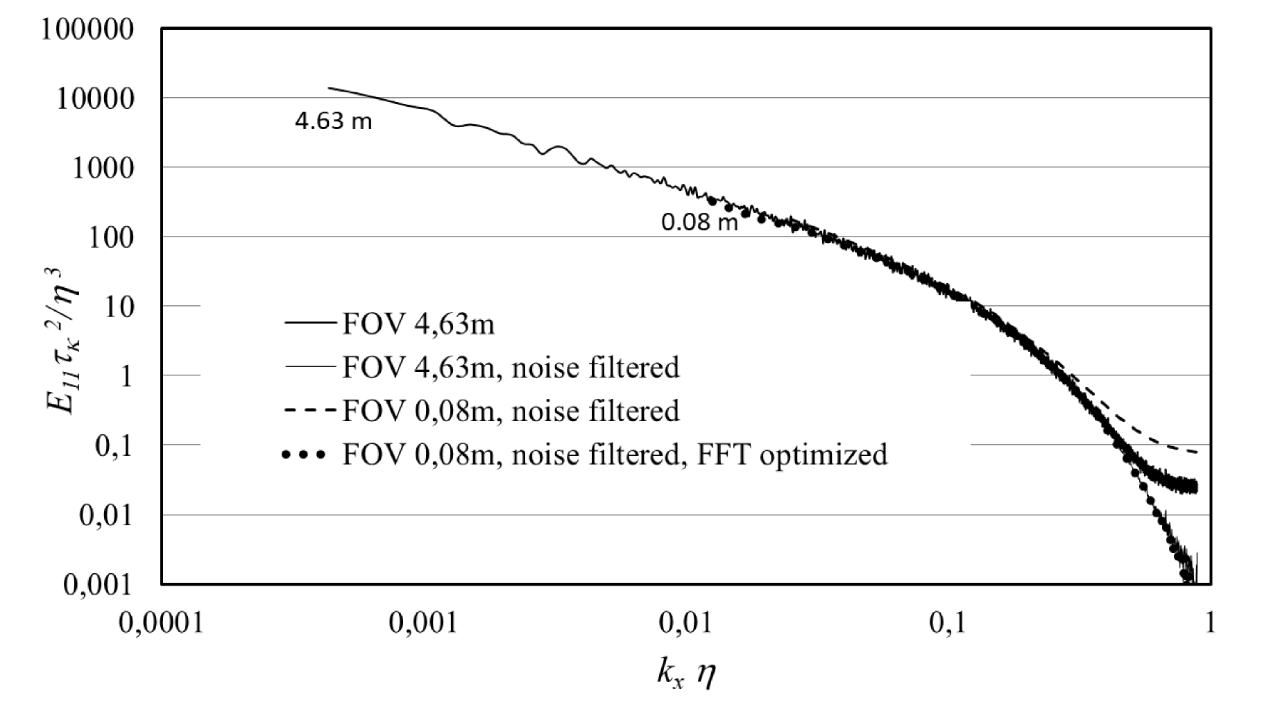
Figure 7 illustrates this effect on an equivalent HW signal for which the spectrum is first computed on long samples of 2 s (corresponding to a window length of 4.63 m). The presence of the HW electronic white noise is visible at high wave numbers and can be removed by a filter or by substraction. Also shown on the figure is the spectrum computed on short samples comparable in size to the present PIV field which is 0.12 m in length (based on Taylor hypothesis). The result is quite poor if no special precaution is taken. A significant leakage occurs from the low wave numbers to the high ones. In the present contribution, the data were processed using a methodology equivalent to several Parzen windows (Foucaut et al. (2004)). Figure 7 shows that this brings a significant improvement to the spectrum for a limited field of view which is close to the original one. The large scales cannot of course be recovered, but the spectrum is reasonable in the range of interest in this experiment.

Figure 8: Comparison of the streamwise and spanwise velocity spectra from PIV and HWA

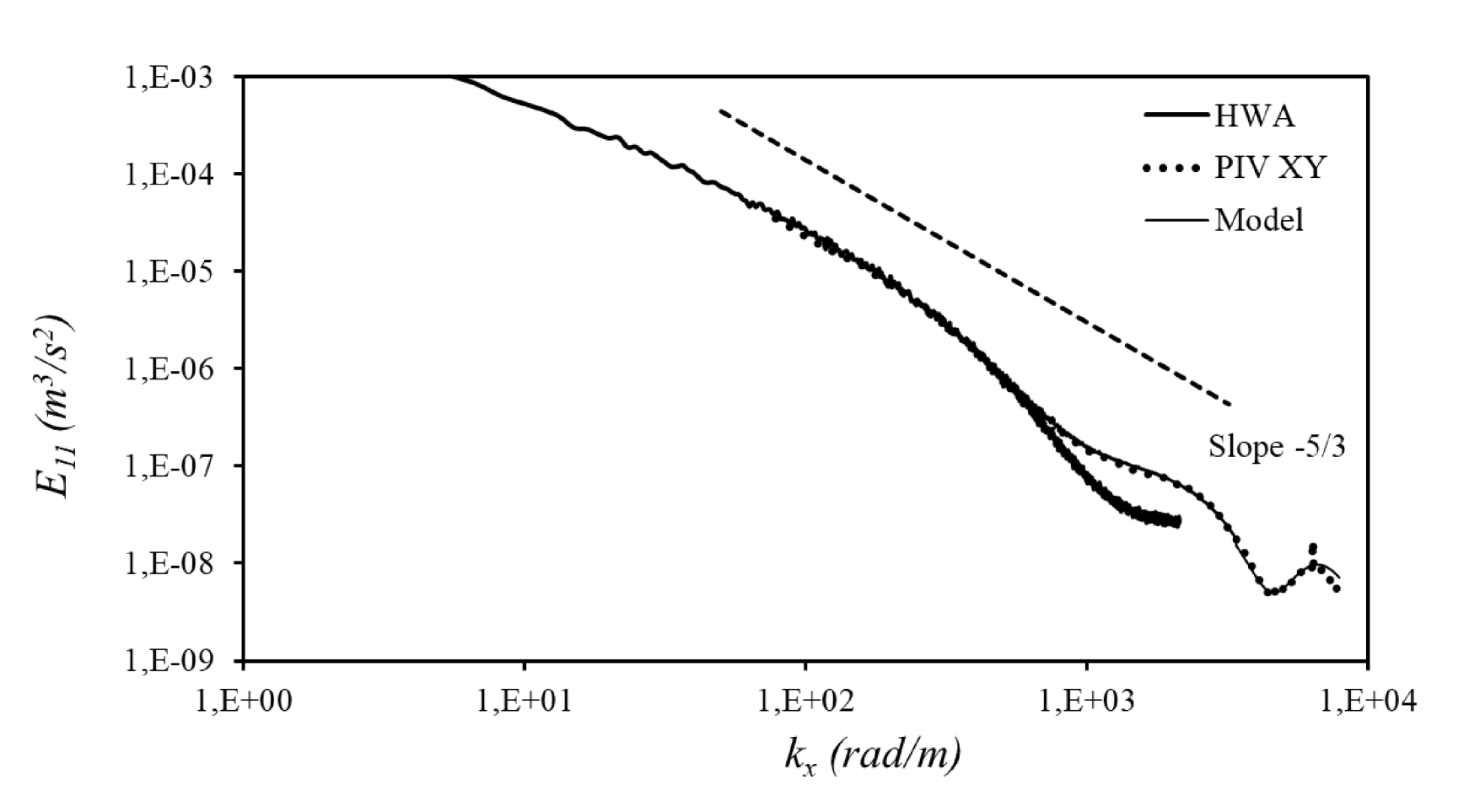
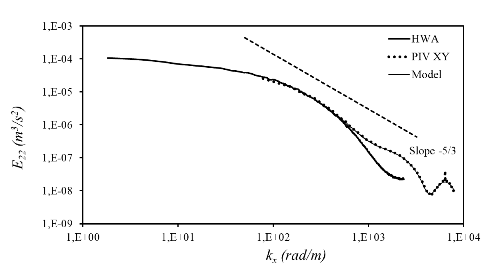
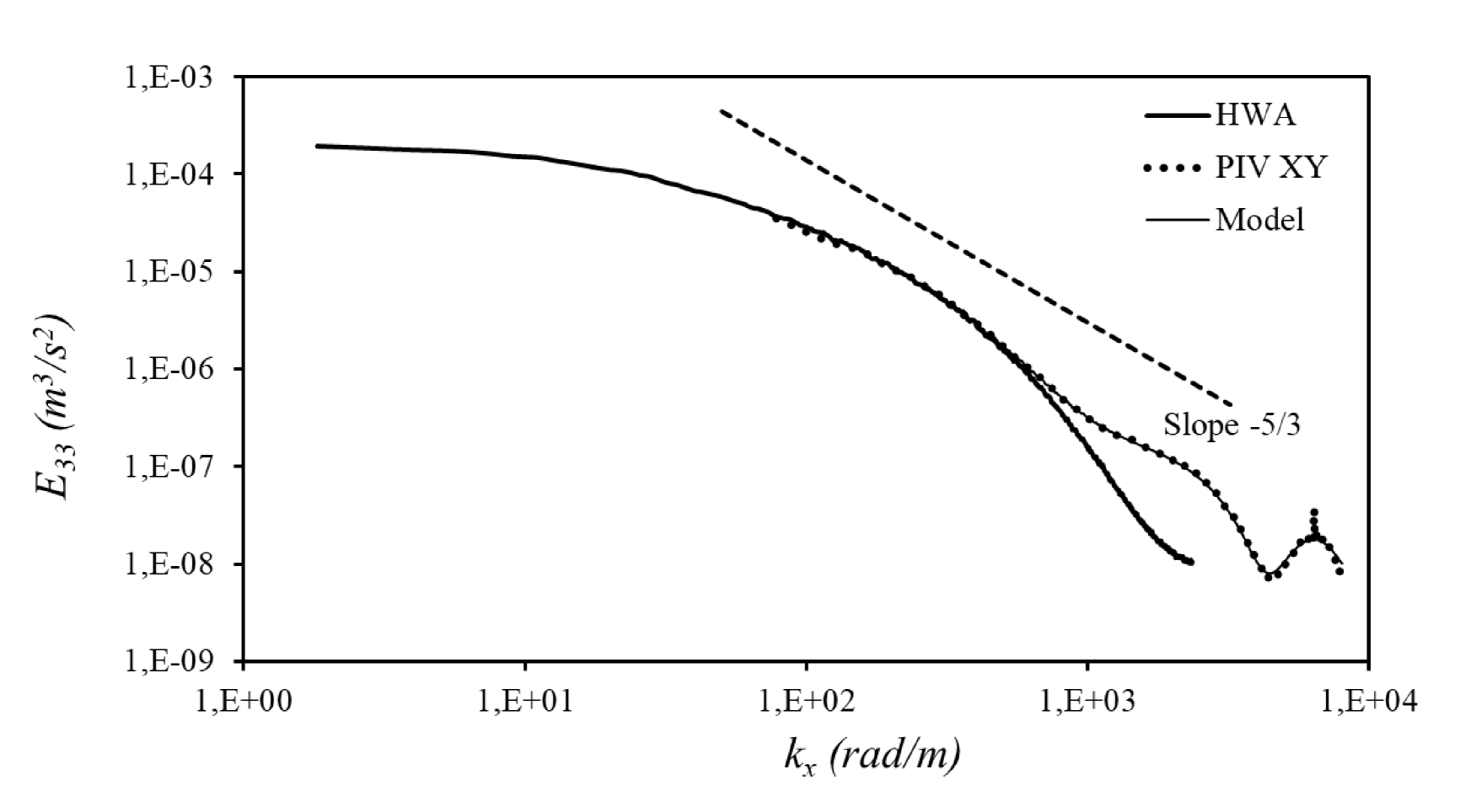
Figure 8 presents now the streamwise, wall-normal and spanwise spectra computed from the streamwise plane SPIV data at a distance of 200 wall units from the wall. Also shown is the HWA ones using a local Taylor hypothesis for the latter. As can be seen, the agreement is excellent below the cut-off frequence $k_{c}$ = 900 rad/m. Above this value, the PIV noise and the effect of the IW size are visible. These will be discussed in more detail in the next section.

The PIV spectrum is compared with the model of Foucaut et al. (2004):

$$E_{11PIV}=(E_{11hw}+E_{noise})\left(\frac{sin(kW\!S/2)}{kW\!S/2}\right)^{2}$$ (3)

which takes into account the effect of a constant white noise and of the interrogation window filtering on the original signal. In this model, $E_{11hw}$ is the “real” turbulence spectrum estimated here by HWA with a Taylor hypothesis, $W\!S$ is the interrogation window size and $E_{noise}$ is obtained by the method described by Foucaut et al. (2004). Note that in Foucaut et al. (2004) a full PIV approach is proposed if the HWA is not available.

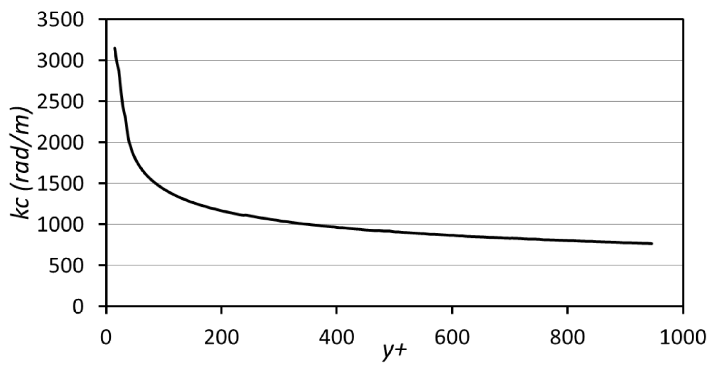
By this approach, the PIV noise level $\sigma_{1}$ on the streamwise component $u_{1}$ can be quantified. From this noise level, the uncertainty on $u_{1}$ can be estimated (Foucaut et al. (2004)). The same approach can be repeated for the two other components. The corresponding values are given in Table 1 for the streamwise plane. The uncertainties on the components stretched and not stretched by the stereoscopic angle are of the order of 0.1 pixel and 0.07 pixel, respectively. These values correspond to a PIV measurement of good quality. Of course, the cut-off frequency of the PIV varies with the distance to the wall. This variation is characterized in figure 9. As will be seen in the next section, it can be taken into account to optimise the derivative filters.

Figure 9: Cut-off wave number $k_{c}$ of the PIV measurements as a function of wall distance.

3.2 Noise assesment

At the intersection of the two PIV planes, the velocity can be estimated by two independent SPIV systems. Along this line, the term $\left\langle u_{i}u_{i}\right\rangle$ can be computed in the streamwise or in the spanwise plane or by the product of $u_{i}$ in each plane. As the two SPIV systems are independent and look at the particles from different angles, the noise can be considered uncorrelated between them. This combined product is then quite interesting as it is free from noise. This gives:

$$\langle u_{i}\left|{}_{(x_{1},x_{2})}\right.u_{i}\left|{}_{(x_{1},x_{2})}\right.\rangle=\langle u_{i}\left|{}_{(x_{1},x_{2})}\right.u_{i}\left|{}_{(x_{3},x_{2})}\right.\rangle+\left(\sigma_{u_{i}}\left|{}_{(x_{1},x_{2})}\right.\right)^{2}$$ (4)

Since the first two terms are measured directly, the uncertainty $\sigma_{u_{i}}$ can be estimated. Figure 10a shows the profiles of these estimations. In the plane ($x_{1},x_{2}$), the value of $\sigma_{u_{i}}$ is relatively constant for $y>5\;mm$. It increases slowly with increasing with $x_{2}$ in the plane ($x_{3},x_{2}$), probably due to an increasing loss of pairs in such a cross-flow plane SPIV when $x_{2}$ (and the mean velocity) increases (v.  Foucaut et al. (2014)). Close to the wall, the uncertainties increases because of the strong mean velocity gradient even if a deformation technique is used.

Figure 10: Estimation of the measurement errors at the intersection line of the two cross-planes.

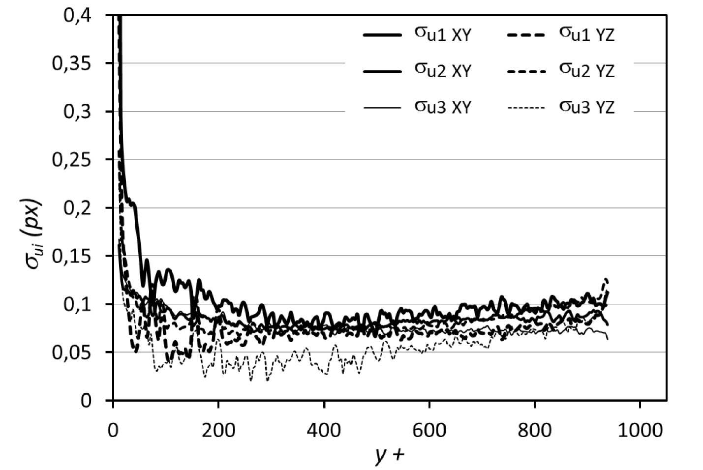
An average of the values for $x_{2}>5\;mm$ was computed for each component and each plane. These values are included in Table 1. For the plane ($x_{1},x_{2}$) they are of the same order as the ones deduced from the spectral analysis. For the plane ($x_{3},x_{2}$) the values are smaller showing a very good quality of measurement for a plane normal to the flow. The errors on the $u_{3}$ component are a little smaller (0.036 pix) than the other two because this component is not stretched in this plane. The measurement uncertainties are finally smaller than 0.1 pixel everywhere, which is representative of a good quality in both planes.

By analogy with equation (4), we can define $\Delta u_{i}u_{j}$ by:

$$\Delta u_{i}u_{j}=\left\langle\left.u_{i}\right|_{(x_{1},x_{2})}\left.u_{j}\right|_{(x_{1},x_{2})}\right\rangle-\left\langle\left.u_{i}\right|_{(x_{1},x_{2})}\left.u_{j}\right|_{(x_{3},x_{2})}\right\rangle$$ (5)

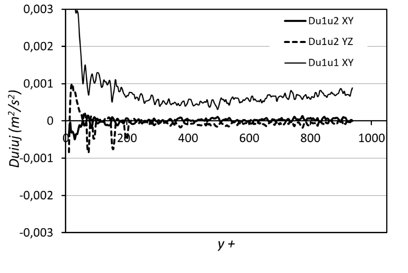
Figure 10b show a comparison of $\Delta u_{1}u_{2}$ for each plane and $\Delta u_{1}u_{1}=\left(\left.\sigma_{u_{i}}\right|_{(x_{1},x_{2})}\right)^{2}$). The values of $\Delta u_{1}u_{2}$ are close to zero for each plane. This is due to the fact that the noise from two different components is not correlated which is not the case for $\Delta u_{1}u_{1}$.

Table 1: Noise level and uncertainties of the SPIV measurement, $E_{noise}$ is the noise level (see Foucaut et al. (2004)), $W\!S$ is the PIV window size and $\sigma_{u}$ is the PIV measurement uncertainties

Plane	Component	$E_{noise}(m^{3}/s^{2})$	$\sigma_{u}$ SP (pix)	$\sigma_{u}$ Dif. (pix)
$x_{1},x_{2}$	$u_{1}$	$1.0\;10^{-7}$	0.076	0.092
$x_{1},x_{2}$	$u_{2}$	$2.2\;10^{-7}$	0.069	0.078
$x_{1},x_{2}$	$u_{3}$	$2.1\;10^{-7}$	0.068	0.079
$x_{3},x_{2}$	$u_{1}$			0.064
$x_{3},x_{2}$	$u_{2}$			0.073
$x_{3},x_{2}$	$u_{3}$			0.036

4 Derivatives computation

The next step toward the characterization of the TKE dissipation is to evaluate the spatial derivatives of the velocity field. Before entering into the details of the approach used here, it is of interest to try to understand and characterize the effect the PIV interrogation window (IW) on the resolution of the dissipative scales.

4.1 Interrogation window size and resolution

For the purpose of understanding the effect of the IW size on the spatial resolution, it is possible to use the HW signal which was recorded on long samples (2 s) and with a good temporal resolution (2.2 kHz). On the basis of a Taylor hypothesis this resolution corresponds at $y^{+}=200$ to 0.88 mm that is 2.5 Kolmogorov units and at $y^{+}=45$ to 0.72 mm that is 2.2 Kolmogorov units. With such a signal, it is possible to simulate the effect of the IW. Before doing that, it is necessary to remove from the HW spectrum the low white noise so that the $k^{2}E(k)$ dissipation spectrum goes effectively to zero at high wave numbers.

(a)                                             (b)

Figure 11: Simulation of the effect of the PIV interrogation window size IW on the attenuation of the dissipation spectra at two wall distances $y^{+}=45$ & $200$.

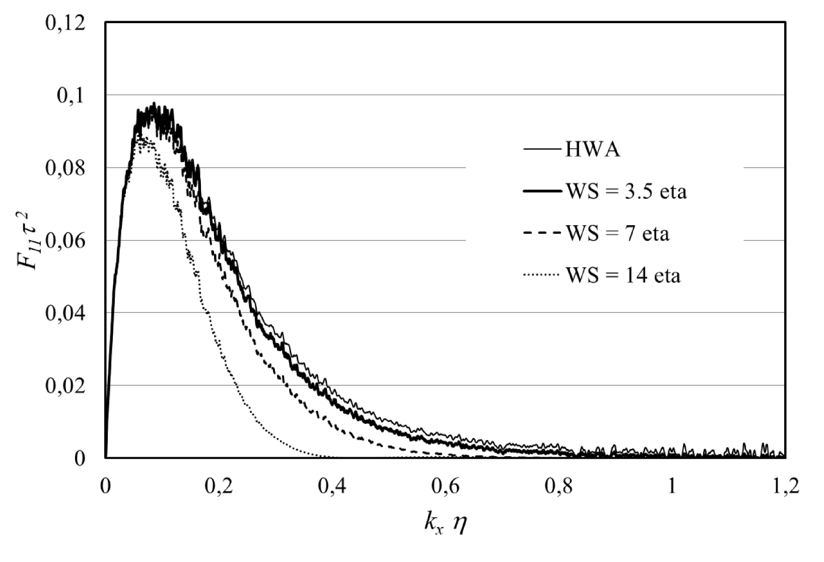
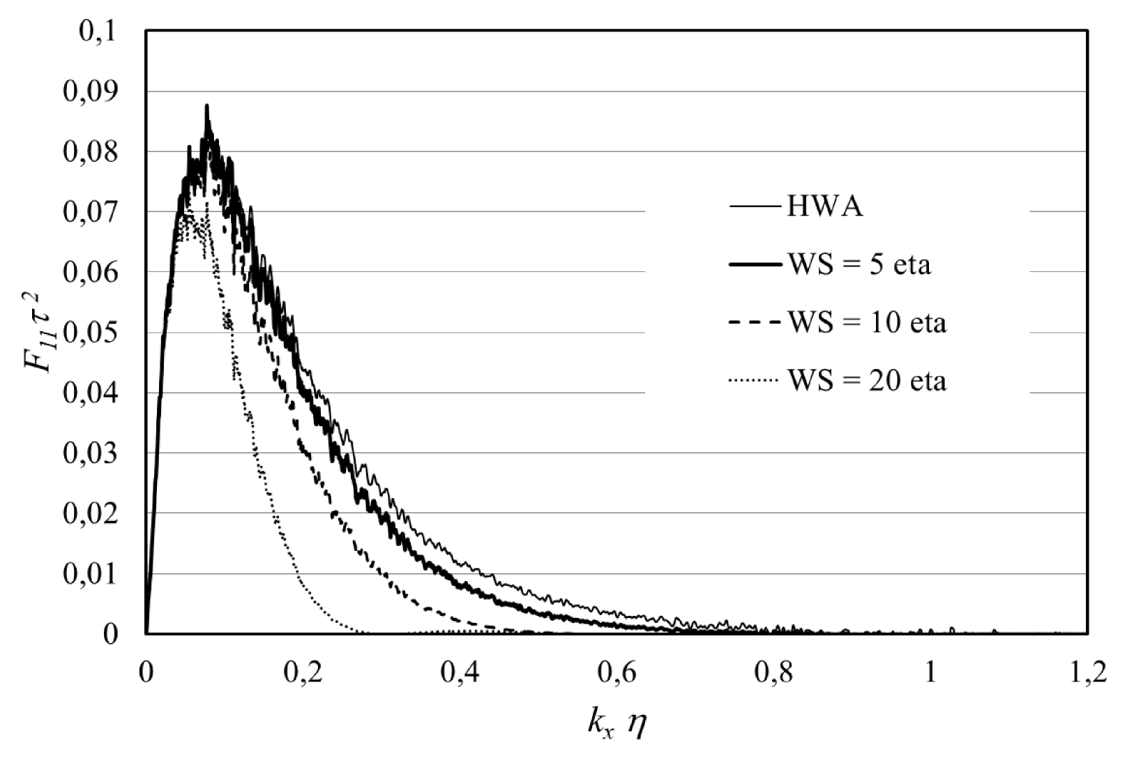
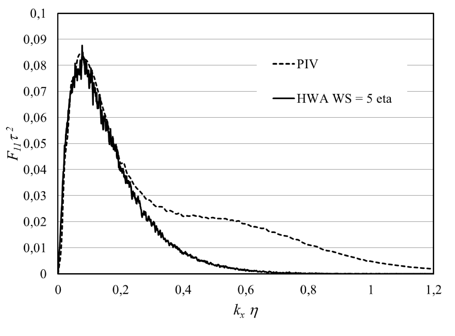
Figure 11 provides the dissipation spectrum $F_{11}$ computed from this HW signal at two wall distances $y^{+}=45$ & $200$ with 3 different values of the interrogation window given in Kolmogorov units (the HW probe was 0.5 mm in length, that is about 1.5 Kolmogorov units, and 2.5 microns in diameter). For comparison, at $y^{+}=45$ the PIV IW is about 5 Kolmogorov units and at $y^{+}=200$ it is about 3. As expected, the reduction of the size of the interrogation window reduces the spatial filtering and provides a better and better estimation of the spectrum. The curves corresponding to 5 and 3 Kolmogorov units at $y^{+}=45$ and $200$ respectively are the closest to the 1.4 mm PIV IW. These are representative of the best possible estimation that the PIV could provide if it was free of noise. With this size of window, the dissipation obtained by integrating the spectrum is about 10 % lower than that provided by the full HW spectrum. These results will be used later to evaluate the derivative estimation approach used in the present study. Note that these estimates are close to those of Lavoie et al. (2007) computed for PIV using DNS spectra and a three-dimensional filter.

4.2 Derivatives computation approach

In the present contribution, the derivatives were computed using the second-order centered-difference scheme proposed by Foucaut and Stanislas (2002). The basic scheme is :

$$\frac{\partial u_{i}}{\partial x_{j}}=\frac{u_{i}^{p+n}-u_{i}^{p-n}}{2n\Delta x_{j}}+\frac{n^{2}\Delta x_{j}^{2}}{2}\frac{\partial^{2}u_{i}}{\partial x_{j}^{2}}+\sigma_{\frac{\partial u_{i}}{\partial x_{j}}}$$ (6)

where $\Delta x_{j}$ is the grid spacing along $x_{j}$. The first term on the right-hand side corresponds to a second order derivative scheme at grid point $p$, the second term corresponds to the truncation error. Increasing the value of n decreases the cut-off frequency of the scheme. The term $\sigma_{\frac{\partial u_{i}}{\partial x_{j}}}=\alpha\frac{\sigma_{u_{i}}}{n\Delta x_{j}}$ is the error due to the noise on the derivative where $\sigma_{u_{i}}$ is the random measurement error on the velocity and $\alpha$ is the quadratic sum of the coefficients used to compute the derivative. Following Foucaut and Stanislas (2002), in the case of a second-order centered-difference scheme, $\alpha=1/\sqrt{2}$. As can be seen, $\sigma_{\frac{\partial u_{i}}{\partial x_{j}}}$ is inversely proportional to the spacing $n\Delta x_{j}$ between the two points used to compute the derivative (Foucaut and Stanislas (2002)). This term is representative of the noise amplification. The higher n, the lower the noise. The choice of n is consequently a compromise between maximizing the cut-off frequency and minimizing the noise. Table 2 gives the values of the cut-off frequency and noise level for $1\leq n\leq 4$. For n = 3 the cut-off frequency of the derivative filter is 925 rad/s which is of the order of the PIV cut-off frequency at $y+=200$ as shown in Figure 8.

Table 2: Characteristics of the derivative schemes

n	$k_{c}$ (rad/m)	$\sigma_{\frac{\partial u_{i}}{\partial x_{j}}}$
1	2800	45.44
2	1350	22.72
3	925	15.15
4	700	11.36

In practice, the measurement noise on the velocities is relatively constant, but the signal level decreases when the wall distance increases. Consequently, to keep a relatively constant signal-to-noise ratio, the cut-off frequency of the derivative scheme has to be reduced. To accomplish that, the derivative can be computed from a combination of central-difference schemes at different orders:

$$\frac{\partial u_{i}}{\partial x_{j}}=\sum_{n=1,4}{a_{n}\frac{u_{i}^{p+n}-u_{i}^{p-n}}{2n\Delta x_{j}}},$$ (7)

where the coefficients $a_{n}$ are optimised as a function of the wall distance to obtain the best cut-off frequencies. The resulting values of $a_{n}$ in the present case are plotted in Figure 12. Figure 13 compares the profiles of $\left\langle\frac{\partial u_{1}}{\partial x_{1}}\frac{\partial u_{1}}{\partial x_{1}}\right\rangle$ computed with n = 1, n = 3 and n optimised. As can be seen, the derivative with the optimisation is in agreement with n = 1 close to the wall and with n = 3 further away.

Figure 12: Evolution of the coefficients $a_{n}$ of equation (7) versus the wall distance.

Figure 13: Profiles of $\left\langle\frac{\partial u_{1}}{\partial x_{1}}\frac{\partial u_{1}}{\partial x_{1}}\right\rangle$ computed with n = 1, n = 3 and n optimised.

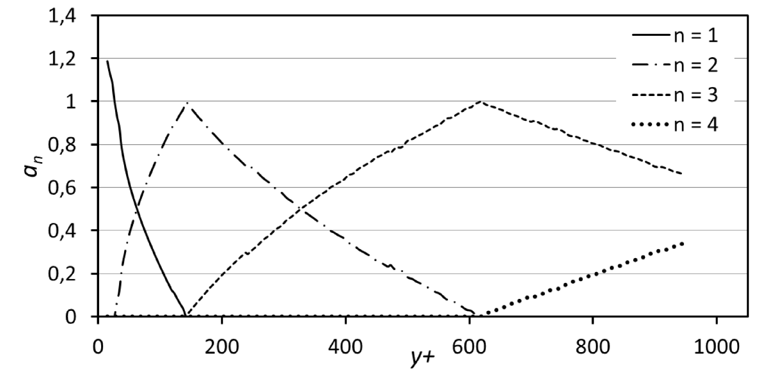
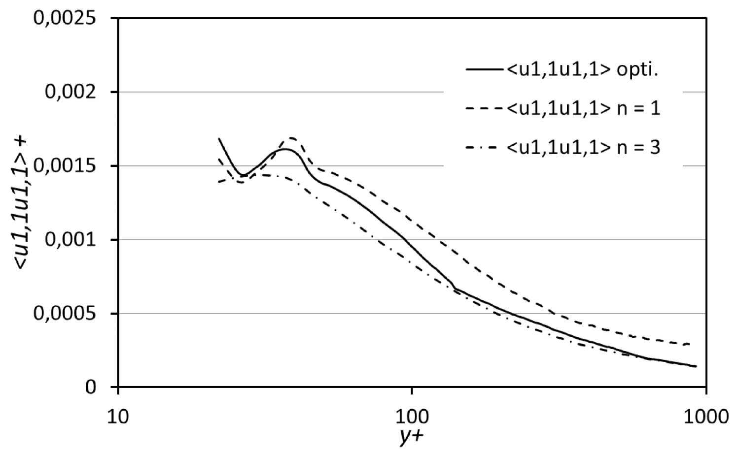
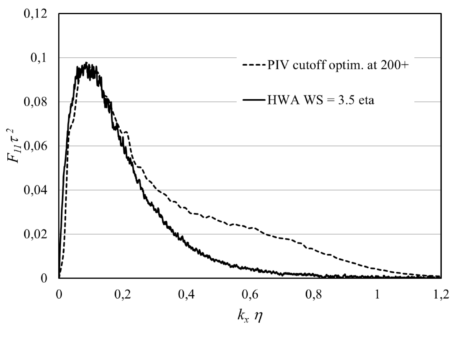
Figure 14 shows a comparison at $y^{+}=45$ and $200$ of the spectrum of $\frac{\partial u_{1}}{\partial x_{1}}$ obtained by the above procedure at $Re_{\tau}=2300$ with the $k^{2}E(k)$ HW spectrum shown already in figure 11. The latter has had the white noise removed and has been computed on windows of 0.12 m and simulating an IW of 3.5 and 5 Kolmogorov respectively. As can be observed, the compromise chosen for the IW and the derivative stencil represents well the peak of the spectrum, but introduces some noise at high frequency. Of course, it would be possible to optimise the derivative filter to bring the PIV spectrum closer to the HW spectrum at high frequency. But this would be at the expense of some signal at the lower frequencies, as the filter does not really distinguish between signal and noise. The choice here was to make a compromise giving a signal-to-noise ratio of one at a cut-off frequency which is close to the velocity fluctuations cut-off frequency. As will be seen below, this remaining noise can be assessed and removed from the derivative moments, thanks to the cross-planes configuration and the use of the continuity equation.

Figure 14: Spectrum of the term $\left\langle\frac{\partial u_{1}}{\partial x_{1}}\frac{\partial u_{1}}{\partial x_{1}}\right\rangle$ compared with a HW simulation at $y^{+}=45$ & $200$.

5 Derivative moments

In order to estimate the dissipation it is required to obtain the derivative moments which appear in equation (2).

5.1 Three methodogies

Thanks to the above, there are three independent methods for computing the derivatie moments. As for the Reynolds stresses, each moment of the type $\left\langle\frac{\partial u_{i}}{\partial x_{2}}\frac{\partial u_{i}}{\partial x_{2}}\right\rangle$ can be computed in the streamwise or in the spanwise plane or by the product of derivative in each plane. The last possibility gives again a result which is free from noise as the noise from the two systems are uncorrelated. By a simple difference, the noise can be estimated:

$$\sigma_{\left.\frac{\partial u_{i}}{\partial x_{2}}\right|_{(x_{1},x_{2})}}^{2}=\left\langle\left.\frac{\partial u_{i}}{\partial x_{2}}\right|_{(x_{1},x_{2})}\left.\frac{\partial u_{i}}{\partial x_{2}}\right|_{(x_{1},x_{2})}\right\rangle-\left\langle\left.\frac{\partial u_{i}}{\partial x_{2}}\right|_{(x_{1},x_{2})}\left.\frac{\partial u_{i}}{\partial x_{2}}\right|_{(x_{3},x_{2})}\right\rangle$$ (8)

A second possibility to estimate the noise is to multiply each normal derivative by the continuity equation:

$$\left\langle\frac{\partial u_{1}}{\partial x_{1}}\frac{\partial u_{1}}{\partial x_{1}}\right\rangle+\left\langle\frac{\partial u_{1}}{\partial x_{1}}\frac{\partial u_{2}}{\partial x_{2}}\right\rangle+\left\langle\frac{\partial u_{1}}{\partial x_{1}}\frac{\partial u_{3}}{\partial x_{3}}\right\rangle=\sigma_{\left.\frac{\partial u_{1}}{\partial x_{1}}\right|_{(x_{1},x_{2})}}^{2}$$

$$\left\langle\frac{\partial u_{2}}{\partial x_{2}}\frac{\partial u_{1}}{\partial x_{1}}\right\rangle+\left\langle\frac{\partial u_{2}}{\partial x_{2}}\frac{\partial u_{2}}{\partial x_{2}}\right\rangle+\left\langle\frac{\partial u_{2}}{\partial x_{2}}\frac{\partial u_{3}}{\partial x_{3}}\right\rangle=\sigma_{\left.\frac{\partial u_{2}}{\partial x_{2}}\right|_{(x_{1},x_{2})}}^{2}$$

$$\left\langle\frac{\partial u_{3}}{\partial x_{3}}\frac{\partial u_{1}}{\partial x_{1}}\right\rangle+\left\langle\frac{\partial u_{3}}{\partial x_{3}}\frac{\partial u_{2}}{\partial x_{2}}\right\rangle+\left\langle\frac{\partial u_{3}}{\partial x_{3}}\frac{\partial u_{3}}{\partial x_{3}}\right\rangle=\sigma_{\left.\frac{\partial u_{3}}{\partial x_{3}}\right|_{(x_{3},x_{2})}}^{2}$$ (9)

Note only the diagonal terms are squared, and that the other terms are relatively noise-free So the latter can be used to calculate a noise-free estimate of the squared terms. As can be seen, the noise $\sigma_{\frac{\partial u_{i}}{\partial x_{i}}}^{2}$ can be estimated from each system.

A third possibility is to follow Foucaut and Stanislas (2002) and to estimate the noise by:

$$\sigma_{\left.\frac{\partial u_{1}}{\partial x_{1}}\right|_{(x_{1},x_{2})}}^{2}=\alpha^{2}\frac{\sigma_{u_{1}}^{2}}{\Delta_{x}^{2}}\sum_{n=1,4}{\frac{a_{n}^{2}}{n^{2}}}$$ (10)

5.2 Comparison of the various methods

Figure 15: Estimation of the random noise error on the derivative $\left\langle\frac{\partial u_{1}}{\partial x_{1}}\frac{\partial u_{1}}{\partial x_{1}}\right\rangle$ by the 2 plane denoising approach and by the continuity.

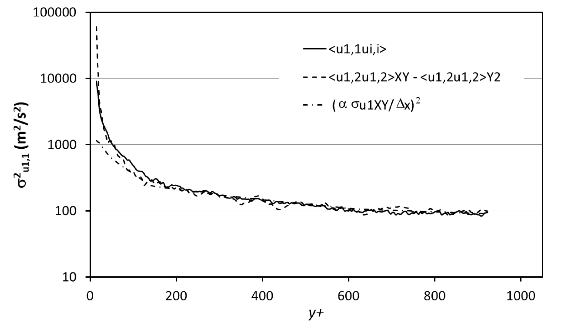
Figure 15 shows the noise error on the derivative $\left\langle\frac{\partial u_{1}}{\partial x_{1}}\frac{\partial u_{1}}{\partial x_{1}}\right\rangle$ obtained from the cross-planes denoising approach (equation (8)), the continuity (equation (9)) and the model of equation (10). These three estimations give sensibly the same results. Therefore they can be used to quantify and remove the noise from the derivative moments. For example, the signal-to-noise ratio for $\left\langle\frac{\partial u_{1}}{\partial x_{1}}\frac{\partial u_{1}}{\partial x_{1}}\right\rangle$ is

$$\sigma_{\left.\frac{\partial u_{1}}{\partial x_{1}}\right|_{XY}}/\sqrt{\left\langle\frac{\partial u_{1}}{\partial x_{1}}\frac{\partial u_{1}}{\partial x_{1}}\right\rangle}\approx 0.6$$

close to the wall and $0.9$ far from the wall for the present configuration. Note that it was about 0.4 and 0.6 at $y^{+}=45$ and $200$ respectively in figure 14 before removing the noise.

Figure 16: Profiles of ${\left\langle\frac{\partial u_{k}}{\partial x_{k}}\frac{\partial u_{i}}{\partial x_{i}}\right\rangle}/{\left\langle\frac{\partial u_{k}}{\partial x_{k}}\frac{\partial u_{k}}{\partial x_{k}}\right\rangle}$ with k = 1, 2 and 3 to verify the continuity.

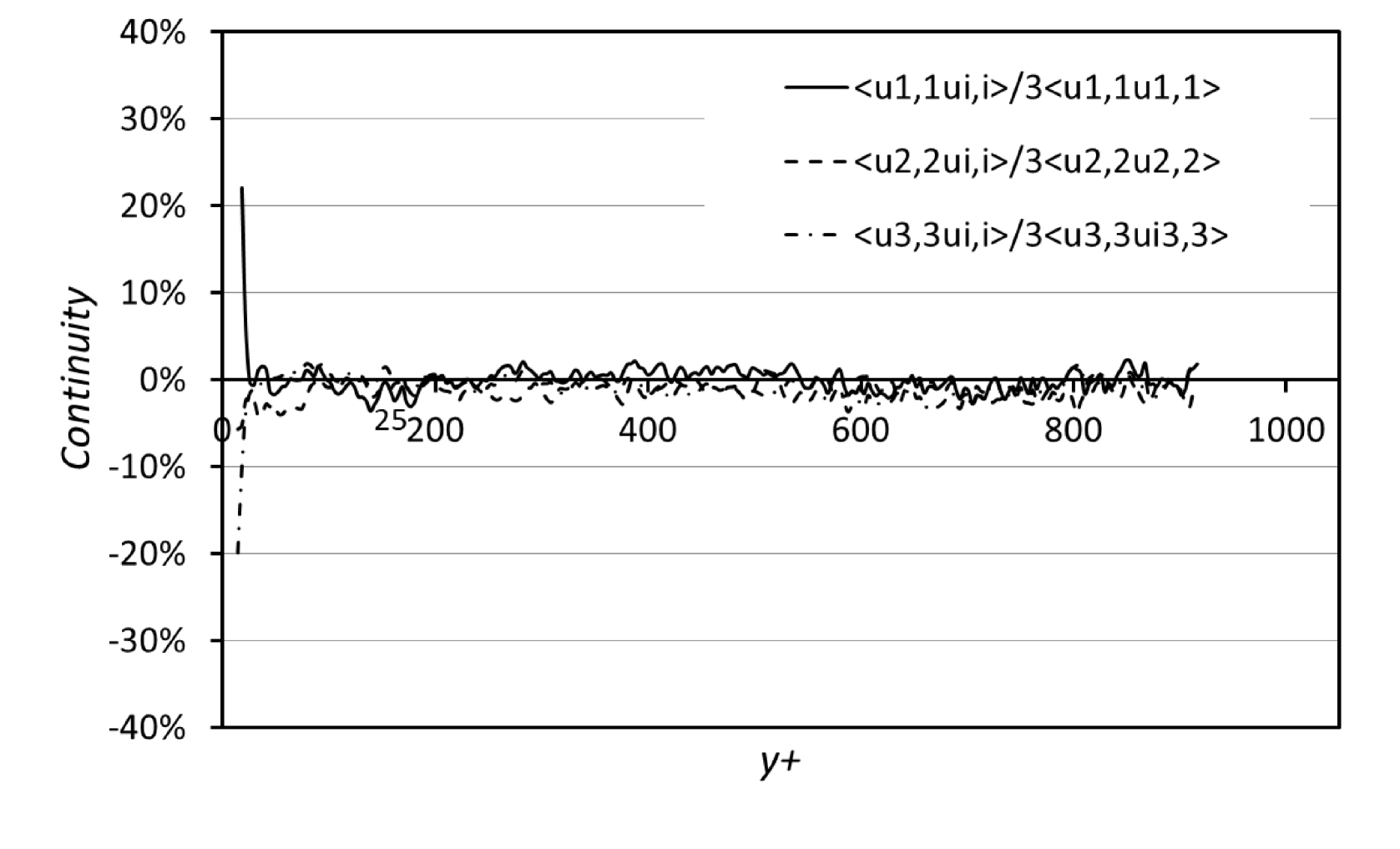
An estimation of the random error can also be obtained after this noise removal by using the continuity equation. Figure 16 shows the profiles of ${\left\langle\frac{\partial u_{k}}{\partial x_{k}}\frac{\partial u_{i}}{\partial x_{i}}\right\rangle}/{\left\langle\frac{\partial u_{k}}{\partial x_{k}}\frac{\partial u_{k}}{\partial x_{k}}\right\rangle}$ for k = 1, 2 and 3 which should verify the continuity. The fluctuations are on the order of 10%. As these data corresponds to the sum of three terms which are random, their value can be divided by $\sqrt{3}$, which gives a random error of the order of 6% on each term. Note that our above simulation with the hot-wire signal gave about 10%.

5.3 The derivative moment data

Figure 17: Comparison of each derivative variance with DNS.

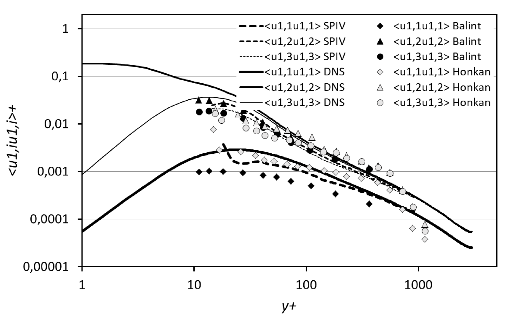
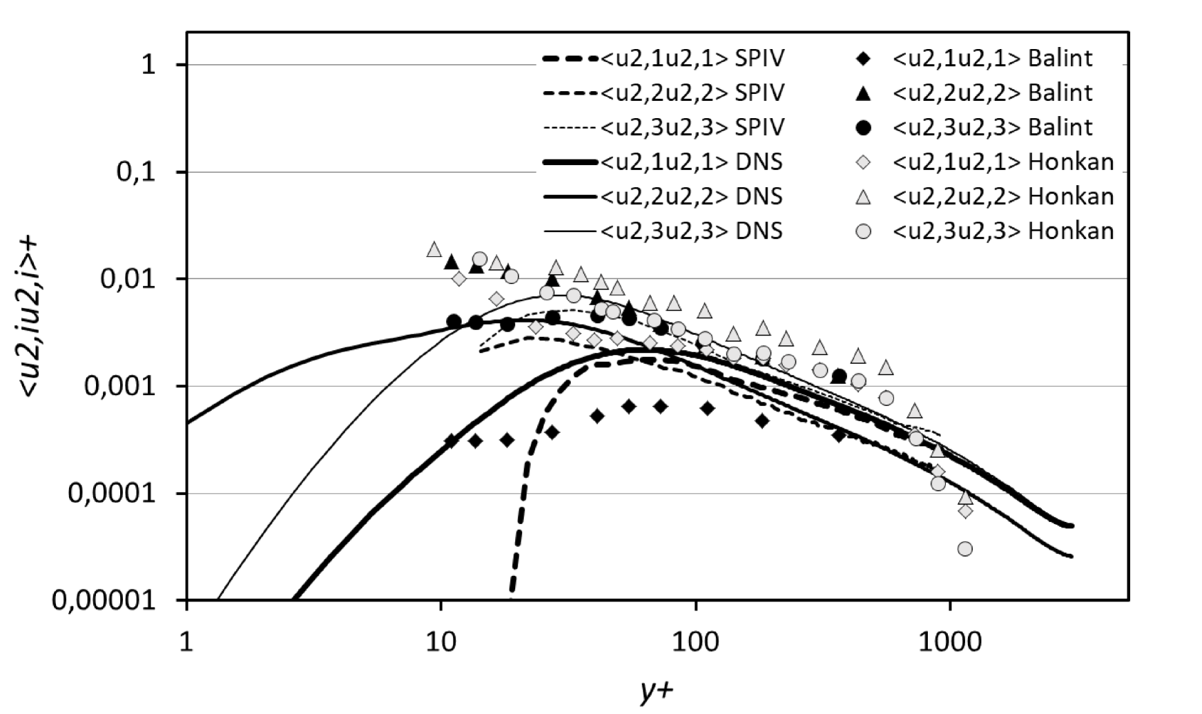
All the derivative moments of equation (2) were computed by the method described in section 4. The term $\left\langle\frac{\partial u_{3}}{\partial x_{1}}\frac{\partial u_{1}}{\partial x_{3}}\right\rangle$ had to be computed at the intersection of the two SPIV planes and could not be averaged along one of the two planes; so it shows a lower level of convergence. Also plotted in figures 17 and 18 are the results from the DNS of a channel flow of Thais et al. (2011) at a comparable Reynolds number. These results are used extensively in parts I and II to analyse the near wall dissipation, so they need not be discussed in detail here.

Figure 18: Comparison of each derivative covariance with DNS.

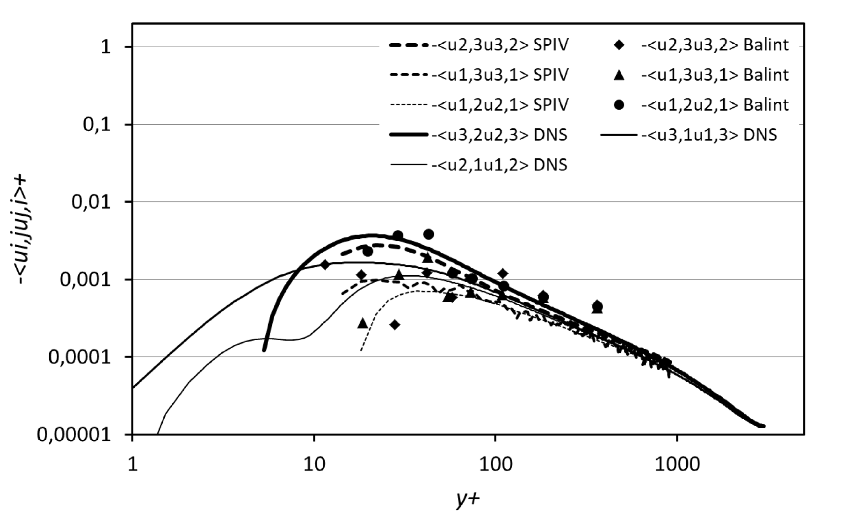
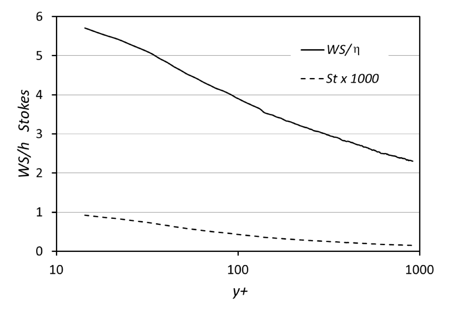
Close to the wall the present results clearly underestimates the derivative moments compared to the DNS. This is due to a filtering of the smaller scale as was shown in section 2 and as is illustrated by figure 19 which gives the size of the interrogation window IW compared to the Kolmogorov length scale $\eta$. This gives a clear indication of the level of spatial filtering due to the PIV interrogation window size. This will be revisited in the conclusion to provide some guidelines for performing PIV experiments with an improved assesment of the derivatives moments.

Figure 19: Interrogation window size normalized by the Kolmogorov micro-scale, $(\nu/\varepsilon)^{1/4}$ and the particle time scale normalized by the Kolmogorov micro-time, $(\nu/\varepsilon)^{1/2}$ as a function of wall distance normalized by $\nu/u_{\tau}$.

6 Some new theoretical considerations

Clearly, measuring the dissipation components in a turbulent flow with PIV is not straightforward. Much care has to be taken both in the set-up of the experiment and in the processing of the PIV data to come to usable results. The challenges presented by the above experiment and the data produced led many discussions among the authors; and these resulted in the recent theoretical contribution by George and Stanislas (2020) which revisited the theory of the PIV measurement and of the associated noise. It is not the place here to redevelop this theory, but it is of interest to give the main results, and use them to bring more insight into the present contribution.

Only the results of interest to the present study are included here, all the details can be found in George and Stanislas (2020) and a summary of the approach in Appendix A. The first important result relevant for the present analysis is the model of one-dimensional spectrum:

$$E_{1,1PIV}(k_{1})=\left({E}_{1,1}(k_{1})+\frac{1}{N}\left\{\langle{u^{\prime}_{1}}^{2}\rangle+\frac{\Delta^{2}}{12}\right\}\frac{\Delta_{1}}{2\pi}\right)\left[\frac{sin(k_{1}\Delta_{1}/2)}{k_{1}\Delta_{1}/2}\right]^{2}$$ (11)

where $E_{1,1PIV}(k_{1})$ is the measured spectrum, ${E}_{1,1}(k_{1})$ is the real volume-averaged spectrum, $N$ is the number of particles in the interrogation volume, $\langle{u^{\prime}_{1}}^{2}\rangle$ is the streamwise Reynolds stress, $\Delta$ is the quantization of the particle images when digitized by the CCD or CMOS and $\Delta_{1}$ is the size along $x_{1}$ of the interrogation volume. This equation is exactly equation (3) with:

$$E_{noise}=\frac{1}{N}\left\{\langle{u^{\prime}_{1}}^{2}\rangle+\frac{\Delta^{2}}{12}\right\}\frac{\Delta_{1}}{2\pi}$$ (12)

As can be seen, $E_{noise}$ is no more a parameter to be adjusted empirically using the data, but one that can be predicted if the turbulence intensity is known. George and Stanislas (2020) came to the conclusion that $\Delta=0.5$ is quite representative of particle images quantization error.

A second interesting result of the theory is the prediction of the noise on the fluctuating velocity moments:

$$\sigma_{i}^{2}=\frac{1}{N}\left\{\langle u^{\prime}_{i}u^{\prime}_{i}\rangle+\frac{1}{12}\Delta^{2}\right\}W(U_{i}\delta t)$$ (13)

where $\sigma_{i}$ is the noise variance on the $i^{th}$ component (no summation on $i$) and $W=\displaystyle\prod_{i=1}^{3}(1-\frac{U_{i}\delta t}{\Delta_{i}})$ is the windowing function which acts only if window shifting is used in the PIV analysis.

The results above can be substituted directly into the noise parameter $\zeta$ (or $E_{noise}$) through the integration of the spectrum as detailed by Foucaut et al. (2004):

$$\zeta_{th}=\frac{\sigma^{2}\Delta_{1}\Delta_{2}}{4I}$$ (14)

where $I=1,492$ is the integral over $[0,2\pi]$ of the “sinc” function and $\Delta_{1}$ and $\Delta_{2}$ are the dimensions of the interrogation window in $mm$ ($X$ and $Y$ in Foucaut et al. (2004) notation).

The last result of this theory is that the noise on the derivative moments is twice the noise on the velocity moments:

$$\xi_{ik}=\frac{2}{N}\left\{\langle u^{\prime}_{i}u^{\prime}_{k}\rangle+\frac{1}{12}\Delta^{2}\delta_{ik}\right\}W(U_{i}\delta t)$$ (15)

Based on these equations, and on the parameters of the experiment, it is possible to compare the noise obtained from the above data analysis with the predictions of the theory. This is done in Table 3 for the $x_{1},x_{2}$ configuration given in Table 1:

Table 3: Noise characteristics, comparison between the theory and the data for the $x_{1},x_{2}$ plane

Comp.	IW	Pixels	N	$u_{i}u_{i}$	$\Delta$	W
$u_{1}$	32x24	768	23.04	0.062	0.0007	0.75
$u_{2}$	32x24	768	23.04	0.018	0.0007	1.00
$u_{3}$	32x24	768	23.04	0.026	0.0007	1.00
$\sigma_{SP}$	$\sigma_{Dif}$	$\sigma_{th}$	$Ratio_{1}$	$\zeta$	$\zeta_{th}$	$Ratio_{2}$
0,020	0.025	0.045	1,83	1.4E-10	6.63E-10	4.73
0,030	0.034	0.028	0,82	3.08E-10	2.57E-10	0.83
0,029	0.034	0.034	0,98	2.94E-10	3.71E-10	1.26

where IW is the size of the interrogation window in pixels, Pixels is the number of pixels in the IW, N is the number of particles inside the IW based on $N_{p}=0.03$, $u_{i}u_{i}$ is the Reynolds stress in $m^{2}/s^{2}$ corresponding to the component, $\Delta$ is the quantization error on the particle images in $m$, $W$ is the windowing coefficient, $\sigma_{SP}$ is the noise variance in $m/s$ obtained from the spectrum analysis, $\sigma_{Dif}$ is the noise variance obtained from the difference between the two planes and $\sigma_{th}$ is the theoretical value given by equation (13), $Ratio_{1}=\sigma_{th}/\sigma_{Dif}$, $\zeta$ is the noise parameter in SI units deduced from the spectrum analysis, $\zeta_{th}$ is the value provided by equation (14) and $Ratio_{2}=\zeta_{th}/\zeta$.

As can be seen in this table 3, the prediction is relatively good along $x_{2}$ and $x_{3}$, while the noise level is overestimated along $x_{1}$. This difference can be explained by the fact that the theory does not take into account the window deformation approach used for the PIV analysis. In the present flow, this technique affects mostly the streamwise component of the Reynolds stress. Taking this point into consideration, the predictions provided in table 14 appear quite satisfactory. Although the theory was developed for 2D2C PIV, it seems to apply also to Stereo PIV if precaution is taken to make the calculations in the physical space (the image space undergoing deformation).

The main interest of this theoretical approach is that it brings into light the sources of noise in the turbulence PIV data and consequently the way to minimize them. The two main sources are the velocity fluctuations inside the interrogation window and the quantization error when the particle images are digitized by the camera sensor. It appears in George and Stanislas (2020) and here that the former is generally dominating the later. Looking at equation 13, the only parameters on which we can act are the number of particle $N$ in the interrogation window and the windowing coefficient $W$. The second one can affect only the Reynolds stress component in the direction of the mean flow and implies minimizing the overlap between the two shifted windows by adjusting their size and the dynamic range (by adjusting the PIV $\delta t$). The effect of the number of particles is relatively slow (as $1/N$), and is limited by the need to keep the particle images separated from each other. It calls nevertheless for a finer tuning of the particle concentration $N_{P}$ during the experiment. Finally, if the objective is to access velocity gradients statistics, a joint optimization of the magnification and of the IW size must be looked for.

7 Summary and Conclusions

From the experimental point of view, measuring the dissipation is a tremendous challenge. Both because it occurs mostly at small scales, and because it involves only derivatives of the velocity field. Measuring it very near a wall is even harder due to the strong mean velocity gradient involved. The aim of the present contribution was to obtain the best possible assessment of the turbulence dissipation near a wall using SPIV. For that purpose, a joint numerical and experimental approach was used. An SPIV experiment was performed in the LMFL boundary layer wind tunnel. And also the results of a plane channel flow DNS at a comparable Reynolds number were used for comparison and validation. The DNS was especially valuable for providing complementary information to the experiment, especially very near the wall.

The main problem of PIV is the limited dynamic range of the technique and the relatively high level of noise. This is not so much a problem when looking at the large scales, but it becomes a real challenge when trying to assess the dissipation, due to the shape of the turbulence spectrum which decreases extremely fast toward the high wave numbers. This means that at the dissipative scales the signal-to-noise ratio becomes a critical issue. The present results show that each stage of the experiment and data processing has to be optimized in order to obtain a reasonable estimation of the dissipative terms.

First of all, the spatial resolution is a key issue. In the present experiment the interrogation window size was varying between roughly 2 and 5 Kolmogorov units from the outer part of the field to the near wall. The results show that some spatial filtering could not be avoided; and if the experiment were to be repeated, staying below 3 Kolmogorov and even close to 2 would be much better. This is quite demanding. In the same conditions, the interrogation window would be close to 0.5 mm in the flow. Luckily, PIV cameras are making continuous progress and this would not be today at the expense of the field-of-view.

Second of all, the optimisation of the interrogation window size in terms of spectral filtering. The method of Foucaut et al. (2004) optimizes the spectral response. It’s extension here to the derivative filter minimizes the noise without losing signal. But, to keep this signal, the data are still quite noisy even after these two steps. This is where the cross-planes SPIV set-up and the exploitation of the continuity equation made the difference. These two tools allowed an accurate characterization of the noise on the derivative moments and the removal of this noise, leading to results which were only limited by the spatial resolution. Thanks to this approach, a good agreement was obtained with the DNS and the differences could be explained, leading to a good cross-validation of the two approaches and to an interesting complementarity of the data.

Besides, thanks to the thinking and exchanges around these data, George and Stanislas (2020) were able to develop a theory explaining and predicting the noise in PIV measurements. This theory, derived for 2D2C PIV, was applied here nevertheless to the SPIV data, and gave results which are quite comforting in terms of the assessment of the noise level in the data generated by this experiment. This new theory will surely become an interesting tool to help in minimizing the noise in PIV measurements.

On the basis of the above analyses and results and of the confidence it gave us in our data, parts I & II of the present contribution (Stanislas et al. (2020); George et al. (2020)) allowed us to analyse in detail the dissipation of both the Turbulence Kinetic Energy and the Reynolds stresses in near wall turbulence, and to come to some conclusion about their origin and behaviour near a solid wall. As shown extensively in part I, the best results of the literature compare quite favourably with the present contribution (Stanislas et al. (2020)).

Appendix A Appendix

As any measuring tool has a limited spatial resolution, the goal of a turbulence experiment is to measure at best the instantaneous volume-averaged Eulerian velocity, say:

$$\tilde{u}_{i}(\vec{y},t)=\frac{1}{V}\int{u_{i}}(\vec{x},t)w(\vec{y},\vec{x}-\vec{y})d\vec{x}$$ (16)

where $y$ is the position vector of the center of the measuring volume, $V$ is the volume, $u_{i}(\vec{x},t)$ is the local Eulerian velocity and the $\tilde{}$ represents volume-averaged quantities. The weighting function $w(\vec{y},\vec{x}-\vec{y})$ defines the measuring volume which, for PIV, can be approximated as a three-dimensional top-hat function. Note that all the fluid particles in the volume contribute equally to the integral. Also in the limit, as $V\rightarrow 0$, $w(\vec{y},\vec{x}-\vec{y})/V\rightarrow\delta(\vec{y})$, so the volume-averaged velocity tends toward the point velocity as the volume shrinks to a point.

In the case of PIV, we do not have access to this volume-averaged velocity as the recorded information is the image of a limited number of particles (usually about 10) inside an interrogation volume at two instant of time. The idea of George and Stanislas (2020) was to represent this ”PIV” instantaneous velocity ${u}_{oi}(\vec{y},t)$ as:

$${u}_{oi}(\vec{y},t)=\frac{1}{N(\vec{y})}\int_{allspace}{v_{i}}(\vec{a},t)w(\vec{y},\vec{X}[\vec{a},t]-\vec{y})g(\vec{a})d\vec{a}$$ (17)

where $N(\vec{y})=\langle n(\vec{y},t)\rangle=\mu V(\vec{y})$ is the average number of particles in the measurement volume at $y$, $\mu$ is the particle concentration, $V(\vec{y})$ is the volume and ${v_{i}}(\vec{a},t)$ is the individual particle Lagrangian velocity, function of the Lagrangian coordinate $a$ and time $t$. The function $g(\vec{a})$ is a random locator function giving the initial Lagrangian position of the particles present in the measurement volume at time $t$. It can be represented as a finite sum of delta functions.

Two important concepts were introduced by George and Stanislas (2020): first the use of generalized functions and second the Lagrangian representation of the particles. Based on these concepts, it was possible to develop single and two points statistics, Reynolds stresses and spectra and to explicit the noise contributing to the difference between the PIV measurement and the volume averaged quantity.

References

- Adrian [1997] R. J. Adrian. Dynamic ranges of velocity and spatial resolution of particle image velocimetry. Measurement Science and Technology, 8(12):1393–1398, 1997.
- Adrian et al. [2000] R.J. Adrian, C.D. Meinhart, and C.D. Tomkins. Vortex organization in the outer layer of the turbulent boundary layer. J. Fluid Mech., 422:1–54, 2000.
- Carlier and Stanislas [2005] J. Carlier and M. Stanislas. Experimental study of eddy structures in a turbulent boundary layer using particle image velocimetry. J. Fluid Mech., 535:143–188, 2005.
- Coudert and Schon [2001] S. Coudert and J. P. Schon. Back projection algorithm with misalignment corrections for 2D3C Stereoscopic PIV. Measurement Science and Technology, 12:1371–1381, 2001.
- Foucaut and Stanislas [2002] J. M. Foucaut and M. Stanislas. Some considerations on the accuracy and frequency response of some derivative filters applied to PIV vector fields. Measurement Science and Technology, 13:1058–1071, 2002.
- Foucaut et al. [2004] J. M. Foucaut, J. Carlier, and M. Stanislas. PIV optimization for the study of turbulent flow using spectral analysis. Measurement Science and Technology, 15:1046–1058, 2004.
- Foucaut et al. [2014] J. M. Foucaut, S Coudert, Braud C., and Velte C.M. Influence of light sheet separation on spiv measurement in a large field spanwise plane. Measurement Science and Technology, 25(3), 2014.
- Foucaut et al. [2011] J.-M. Foucaut, S. Coudert, M. Stanislas, and J. Delville. Full 3d correlation tensor computed from double field stereoscopic piv in a high reynolds number turbulent boundary layer. Experiments in Fluids, 50(4, Sp. Iss. SI):839–846, APR 2011.
- Ganapathisubramani et al. [2005] B. Ganapathisubramani, N. Hutchins, W. T. Hambleton, E. K. Longmire, and I. Marusic. Investigation of large-scale coherence in a turbulent boundary layer using two-point correlations. Journal of Fluid Mechanics, 524:57–80, 2005.
- Ganapathisubramani et al. [2006] B. Ganapathisubramani, E. K. Longmire, and I. Marusic. Experimental investigation of vortex properties in a turbulent boundary layer. Physics of Fluids, 18(055105.114), 2006.
- George and Stanislas [2020] W.K. George and M. Stanislas. On the noise in statistics of PIV measurements. Submitted to experiments in Fluids, 2020.
- George et al. [2020] W.K. George, M. Stanislas, J. M. Foucaut, J. P. Laval, and C. Cuvier. Velocity derivatives in a high Reynolds number Turbulent Boundary Layers. Part 2: Statistical Properties. Submitted to Journal of Fluid Mech., 2020.
- Hambleton et al. [2006] W. T. Hambleton, N. Hutchins, and I. Marusic. Simultaneous orthogonal plane particle image velocimetry measurements in a turbulent boundary layer. Journal of Fluid Mechanics, 560:53–64, 2006.
- Herpin et al. [2012] S. Herpin, S. Coudert, J.-M. Foucaut, and M. Stanislas. Influence of the reynolds number on the vortical structures in the logarithmic region of turbulent boundary layers. Journal of Fluid Mechanics, 716:5–50, 2012.
- Kahler and Stanislas [2000] C. J. Kahler and M. Stanislas. Investigation of wall bounded flows by means of multiple plane stereo PIV. In to appear in the proceedings of the 10th Int. Symp. on Appl. of Laser Tech. to Fluid Mech, Lisbon, 2000.
- Lavoie et al. [2007] G. Lavoie, P. nd Avallone, F. De Gregorio, G. P. Romano, and R. A. Antonia. Spatial resolution of piv for the measurement of turbulence. Exp. in Fluids, 43:39–51, 2007.
- Raffel et al. [1998] M. Raffel, C. Willert, and J. Kompenhans. Particle Image Velocimetry. Springler-Verlag Berlin Heidelberg, 1998.
- Scarano [2002] F Scarano. Iterative image deformation methods in PIV. Measurement Science and Technology, 13(1):R1–R19, 2002.
- Soloff et al. [1997] S. Soloff, R. Adrian, and Z. C. Liu. Distortion compensation for generalized Stereoscopic Particle Image Velocimetry. Meas. Science Tech., 8:1441–1454, 1997.
- Stanislas et al. [2020] M. Stanislas, J. M. Foucaut, W. George, C. Cuvier, and J. P. Laval. Velocity derivatives in a high Reynolds number Turbulent Boundary Layer. Part 1: Dissipation and Energy Balance. submitted to JFM, 2020.
- Stanislas et al. [2007] M Stanislas, K Okamoto, CJ Kahler, J Westerweel, and F Scarano. Main results of the third international PIV challenge. EXPERIMENTS IN FLUIDS, 45(1):27–71, AUG 2007. Sept.19-20, 2005, Pasadena, USA.
- Thais et al. [2011] L. Thais, A. E. Tejada-Martínez, T. B. Gatski, and G. Mompean. A massively parallel hybrid scheme for direct numerical simulation of turbulent viscoelastic channel flow. Comp. & Fluid, 43:134–142, 2011.
- Wieneke [2005] B Wieneke. Stereo-PIV using self-calibration on particle images. Experiments in Fluids, 39(2):267–280, 2005.
- Willert [1997] C. Willert. Stereoscopic digital particle image velocimetry for applications in wind tunnel flows. Measurement Science and Technology, 8:1465–1479, 1997.