An Identifiable Double VAE For Disentangled Representations

Abstract

A large part of the literature on learning disentangled representations focuses on variational autoencoders (vae). Recent developments demonstrate that disentanglement cannot be obtained in a fully unsupervised setting without inductive biases on models and data. However, Khemakhem et al., AISTATS, 2020 suggest that employing a particular form of factorized prior, conditionally dependent on auxiliary variables complementing input observations, can be one such bias, resulting in an identifiable model with guarantees on disentanglement. Working along this line, we propose a novel vae-based generative model with theoretical guarantees on identifiability. We obtain our conditional prior over the latents by learning an optimal representation, which imposes an additional strength on their regularization. We also extend our method to semi-supervised settings. Experimental results indicate superior performance with respect to state-of-the-art approaches, according to several established metrics proposed in the literature on disentanglement.

1 Introduction

Representation learning aims at learning data representations such that it is easier to extract useful information when building classifiers or other predictive tasks (Bengio et al., 2013). Representation learning seeks to obtain the following properties: i) expressiveness: a reasonably-sized representation should allow to distinguish among a high number of different input configurations; ii) abstractness: learned representations should capture high-level features; iii) invariance: representation should be invariant to local changes of input configurations; iv) interpretability: learned representations should allow each dimension to be informative about the given task. These properties are at the core of disentangled representations.

Figure 1: Toy example where each $z_{i}$ controls a given ground-truth factor: $z_{1}$ the size, $z_{2}$ the shape of the 2D objects.

In disentangled representation learning, the main assumption is that high-dimensional observations $\mathbf{x}$ are the result of a (possibly nonlinear) transformation applied to a low dimensional latent variable of independent generative factors, called ground-truth factors, capturing semantically meaningful concepts. Input observations can be thought of as the result of a probabilistic generative process, where latent variables $\mathbf{z}$ are first sampled from a prior distribution $p(\mathbf{z})$, and then the observations $\mathbf{x}$ are sampled from $p(\mathbf{x}|\mathbf{z})$. The goal is to learn a representation of the data that captures the generative factors. In simple terms, illustrated in fig. 1, each dimension of a disentangled representation refers to a single factor of variation.

In this work, we focus on deep generative models, and in particular those based on variational autoencoders (vae), to learn disentangled representations. A well known theoretical result asserts that disentanglement is essentially impossible in a fully unsupervised setting, without inductive biases on models and data (Locatello et al., 2019). However, inducing a disentangled structure into the latent space where z lies is feasible by incorporating auxiliary information u about the ground-truth factors in the model. The type and amount of supervision define different families of disentanglement methods, often classified as supervised, semi-supervised, and weakly-supervised. In most of these methods, the auxiliary variables u become an integral part of the latent space. However, recent work (Khemakhem et al., 2020) indicates that there are alternative strategies to benefit from auxiliary information, such as using it to impose a structure on the latent space. In their proposal, this is done by learning a prior distribution on the latent space, where the crucial aspect is that this is conditioned on auxiliary information $\mathbf{u}$ that is coupled with every input observations. Under mild assumptions, it is possible to show that such form of conditioning implies model identifiability, allowing one to recover the original ground-truth factors and therefore providing principled disentanglement.

In this work, we propose a novel generative model that, like Khemakhem et al. (2020), uses a conditional prior and has theoretical identifiability guarantees. We show that our method naturally imposes an optimality constraint, in information theoretic terms, on the conditional prior: this improves the regularization on the function that maps input observations to latent variables, which translates in tangible improvements of disentanglement in practice. Since assuming to have access to auxiliary variables for each input observations, both at training and testing time, is not practical in many applications, we also propose a semi-supervised variant of our method.

Our Contributions: i) We present a detailed overview of vae-based disentanglement methods using a unified notation. Our focus is on the role of the regularization term. We introduce a distinction between direct matching approaches, in which ground-truth factors are directly matched to the latent space, and indirect matching approaches, where a prior distribution over the latents is used to structure the learned latent space. ii) We design a new method, that we call Identifiable Double vae (idvae) since its ELBO can be seen as a combination of two variational autoencoders, that is identifiabile, in theory, and that learns an optimal conditional prior, which is truly desirable in practice. We additionally propose a semi-supervised version of idvae to make our method applicable also when auxiliary information is available for a subset of the input observations only. iii) We design an experimental protocol that uses four well-known datasets, and established disentanglement metrics. We compare our method to several state-of-the-art competitors and demonstrate that idvae achieves superior disentanglement performance across most experiments.

2 Preliminaries

Let $\mathbf{x}\in\mathbb{R}^{n}$ be some input observations, which are the result of a transformation of independent latent ground-truth factors $\mathbf{z}\in\mathbb{R}^{d}$ through a function $\mathbf{f}:\mathbb{R}^{d}\rightarrow\mathbb{R}^{n}$. Then, we have that $\mathbf{x}=\mathbf{f}(\mathbf{z})+\boldsymbol{\epsilon}$, where $\boldsymbol{\epsilon}$ is a Gaussian noise term: $\boldsymbol{\epsilon}\sim\mathcal{N}(0,\boldsymbol{\Sigma})$, and independent of $\mathbf{z}$. Let consider the following generative model:

$$p_{\boldsymbol{\theta}}(\mathbf{x},\mathbf{z})=p_{\boldsymbol{\theta}}(\mathbf{x}|\mathbf{z})p_{\boldsymbol{\theta}}(\mathbf{z}),$$ (1)

where $\boldsymbol{\theta}\in\boldsymbol{\Theta}$ is a vector of model parameters, $p_{\boldsymbol{\theta}}(\mathbf{z})=\prod_{i=1}^{d}p_{\boldsymbol{\theta}}(z_{i})$ represents the factorized prior probability distribution over the latents and $p_{\boldsymbol{\theta}}(\mathbf{x}|\mathbf{z})$ is the conditional distribution to recover $\mathbf{x}$ from $\mathbf{z}$. The decoder function $\mathbf{f}(\mathbf{z})$ determines the way $\mathbf{z}$ is transformed into $\mathbf{x}$ within $p_{\boldsymbol{\theta}}(\mathbf{x}|\mathbf{z})$.

Assume to observe some data $\mathcal{D}=\{{\mathbf{x}}^{(1)},\cdots,{\mathbf{x}}^{(N)}\}$ generated by $p_{\boldsymbol{\theta}^{*}}(\mathbf{x},\mathbf{z})=p_{\boldsymbol{\theta}^{*}}(\mathbf{x}|\mathbf{z})p_{\boldsymbol{\theta}^{*}}(\mathbf{z})$, where $\boldsymbol{\theta}^{*}$ are the true, but unknown parameters. Then, the goal is to learn $\boldsymbol{\theta}\in\boldsymbol{\Theta}$ such that:

$$p_{\boldsymbol{\theta}}(\mathbf{x},\mathbf{z})=p_{\boldsymbol{\theta}^{*}}(\mathbf{x},\mathbf{z}).$$ (2)

When eq. 2 holds, it is then possible to recover the generative ground-truth factors. Unfortunately, by observing $\mathbf{x}$ alone, we can estimate the marginal density $p_{\boldsymbol{\theta}}(\mathbf{x})\approx p_{{\boldsymbol{\theta}}^{*}}(\mathbf{x})$, but there are no guarantees about learning the true generative model $p_{\boldsymbol{\theta}^{*}}(\mathbf{x},\mathbf{z})$. This is only feasible for models satisfying the following implication:

$$\forall({\boldsymbol{\theta}},{\boldsymbol{\theta}}^{\prime}):p_{\boldsymbol{\theta}}(\mathbf{x})=p_{{\boldsymbol{\theta}}^{\prime}}(\mathbf{x})\Longrightarrow{\boldsymbol{\theta}}={\boldsymbol{\theta}}^{\prime}.$$ (3)

When eq. 3 holds, the estimated and the true marginal distribution match, and their parameters match too. Then, the model is identifiable (Khemakhem et al., 2020) and, as a consequence, it allows one to recover the latent ground-truth factors and obtain a disentangled representation:

$$p_{\boldsymbol{\theta}}(\mathbf{x})=p_{{\boldsymbol{\theta}}^{\prime}}(\mathbf{x})\Longrightarrow p_{\boldsymbol{\theta}}(\mathbf{x},\mathbf{z})=p_{{\boldsymbol{\theta}}^{\prime}}(\mathbf{x},\mathbf{z}).$$ (4)

A practical goal is to aim for model identifiability up to trivial transformations, such as permutation and scaling; as long as ground-truth factors can be identified, their order and scale is irrelevant.

3 Related work

Today, a large body of work to learn disentangled representations is based on generative models. In this work, we focus on vae-based approaches (Kingma & Welling, 2014; Rezende et al., 2014).

Variational Autoencoder. A standard vae learns the parameters of eq. 1 by introducing an inference model $q_{\boldsymbol{\phi}}(\mathbf{z}|\mathbf{x})$ to derive an ELBO as follows:

$$\mathcal{L}_{{\textsc{vae}}}=\mathbb{E}_{q_{\boldsymbol{\phi}}(\mathbf{z}|\mathbf{x})}[\log p_{\boldsymbol{\theta}}(\mathbf{x}|\mathbf{z})]-\mathrm{KL}(q_{\boldsymbol{\phi}}(\mathbf{z}|\mathbf{x})||p(\mathbf{z})),$$ (5)

where, by abuse of notation, we write $\mathbf{x}$ in place of $\mathbf{x}^{(i)}$. This avoids clutter in the presentation of vae-based models, but, clearly, the marginal log-likelihood is composed of a sum of such ELBO terms, one for each observation $\mathbf{x}^{(i)}$ (Kingma & Welling, 2014).

The distribution $p_{\boldsymbol{\theta}}(\mathbf{x}|\mathbf{z})$ has the role of a decoder, whereas $q_{\boldsymbol{\phi}}(\mathbf{z}|\mathbf{x})$ can be seen as an encoder, and it is generally assumed to be a factorized Gaussian with a diagonal covariance matrix. Both distributions are parameterized with neural networks, with parameters $\boldsymbol{\theta}$ and variational parameters $\boldsymbol{\phi}$. The prior $p(\mathbf{z})$ is generally a factorized, isotropic unit Gaussian.

The first term of eq. 5 relates to the reconstruction of the input data using latent variables sampled from the variational approximation of the true posterior. The second term is a regularization term, which pushes the approximate posterior $q_{\boldsymbol{\phi}}(\mathbf{z}|\mathbf{x})$ to match the prior on the latent space. Maximizing eq. 5 across observations implies learning the parameters such that the reconstruction performance is high, and the regularization term is small.

Since both terms that appear in the regularization of eq. 5 are factorized Gaussians with diagonal covariance, one way to interpret the individual components $z_{i}$ of the latent space is to view them as independent white noise Gaussian channels (Burgess et al., 2017). When the $\mathrm{KL}$ term is zero, the latent channels $z_{i}$ have zero capacity: this happens when the approximate posterior $q_{\boldsymbol{\phi}}(\mathbf{z}|\mathbf{x})$ matches exactly the prior $p_{\boldsymbol{\theta}}(\mathbf{z})$. In this case, however, the reconstruction term is penalized. To increase $\mathrm{KL}(\cdot)>0$, it is necessary to decrease the overlap between channels, and reduce their variances.

Unsupervised disentanglement learning. The above understanding of the regularization term is at the basis of many variants of the original vae model, that strive to increase the pressure on the regularization term, or elements thereof, to achieve disentanglement, without sacrificing reconstruction properties too much. For example Higgins et al. (2017) propose $\beta$-vae, which modifies eq. 5 by introducing a hyper-parameter $\beta$ to gauge the pressure on the regularization term throughout the learning process:

$$\mathcal{L}_{\beta-{\textsc{vae}}}=\mathbb{E}_{q_{\boldsymbol{\phi}}(\mathbf{z}|\mathbf{x})}[\log p_{\boldsymbol{\theta}}(\mathbf{x}|\mathbf{z})]-\beta\mathrm{KL}(q_{\boldsymbol{\phi}}(\mathbf{z}|\mathbf{x})||p(\mathbf{z})).$$ (6)

When $\beta>1$, the encoder distribution $q_{\boldsymbol{\phi}}(\mathbf{z}|\mathbf{x})$ is pushed towards the unit Gaussian prior $p(\mathbf{z})$. In light of the discussion above, the strong penalization of the $\mathrm{KL}$ term in $\beta$-vae affects the latent channel distribution, by reducing the spread of their means, and increasing their variances.

Many methods build on $\beta$-vae (Burgess et al., 2017; Kim & Mnih, 2018; Kumar et al., 2018; Chen et al., 2018; Zhao et al., 2019), rewriting the ELBO in slightly different ways. A generalization of the $\mathrm{KL}$ term decomposition proposed by Hoffman & Johnson (2016); Makhzani & Frey (2017) is the following (Chen et al., 2018):

$$\mathbb{E}_{\mathbf{x}}[\mathrm{KL}(q_{\boldsymbol{\phi}}(\mathbf{z}|\mathbf{x})||p(\mathbf{z}))]=$$

$$I(\mathbf{x};\mathbf{z})+\mathrm{KL}(q(\mathbf{z})||\prod_{j}q(z_{j})))+\sum_{j}\mathrm{KL}(q(z_{j})||p(z_{j}))$$

where $q(\mathbf{z})$ is the aggregated posterior and $I(\mathbf{x};\mathbf{z})$ is the mutual information between $\mathbf{x}$ and $\mathbf{z}$. Penalizing $I(\mathbf{x};\mathbf{z})$ can be harmful to reconstruction purposes, but enforcing a factorized aggregated posterior encourages independence across the dimensions of $\mathbf{z}$, favouring disentanglement. The dimensional independence in the latent space is encouraged by the second term, known as total correlation (TC). The third term is a further regularization, preventing the aggregate posterior to deviate too much from the factorized prior.

Note that unsupervised vae-based approaches approximate the data marginal distribution $p_{\boldsymbol{\theta}}(\mathbf{x})$, but there are no guarantees to recover the true joint probability distribution $p_{\boldsymbol{\theta}}(\mathbf{x},\mathbf{z})$, having acces to the input observations $\mathbf{x}$ only (Khemakhem et al., 2020). Pushing the model to learn a representation with statistically independent dimensions is not a sufficient condition to obtain full disentanglement. These considerations were recently formalized in the impossibility result (Locatello et al., 2019), but they were already known in the nonlinear ica literature (Comon, 1994; Hyvärinen & Pajunen, 1999).

Auxiliary variables and disentanglement. To overcome the above limitations, a key idea is to incorporate an inductive bias in the model. The choice of the variational family and prior distribution can be one of such bias (Mathieu et al., 2019; Kumar & Poole, 2020). Alternatively, it is possible to rely on additional information about the ground-truth factors, which we indicate as $\mathbf{u}\in\mathbb{R}^{m}$. When auxiliary observed variables u are available, they can be used jointly with $\mathbf{z}$ to reconstruct the original input $\mathbf{x}$. These methods are usually classified under the semi/weakly supervised family. More specifically Shu et al. (2020) identify three forms of weak supervision: restricted labeling (Kingma et al., 2014; Cheung et al., 2015; Siddharth et al., 2017; Klys et al., 2018), match/group pairing (Bouchacourt et al., 2018; Hosoya, 2019; Locatello et al., 2020a), and rank pairing (Chen & Batmanghelich, 2020a, b). In the extreme case, when all ground-truth factors are known for all the input samples, we label them as supervised disentanglement methods.

As for unsupervised counterpart, methods relying on auxiliary observed variables $\mathbf{u}$ differ in how the regularization term(s) are designed. Some approaches use a “supervised” regularization term to directly match $\mathbf{z}$ and the available ground-truth factors $\mathbf{u}$: we refer to this form of regularization as direct matching. An example is what we here call fullvae method (Locatello et al., 2020b), which optimizes the following ELBO:

$$\mathcal{L}_{{\textsc{fullvae}}}=\mathcal{L}_{\beta\text{-{{vae}}}}-\gamma R_{s}(q_{\boldsymbol{\phi}}(\mathbf{z}|\mathbf{x}),\mathbf{u}),$$ (7)

where $R_{s}(\cdot)$ is a loss function between the latent and the ground-truth factors (in the original implementation it is a binary cross entropy loss). Other approaches employ a $\mathrm{KL}$ divergence term between the posterior and the prior over the latents: we refer to this form of regularization as indirect matching. In other words, direct matching methods require explicit knowledge of one or more ground-truth factors, whereas indirect matching can also use weak information about them. Shu et al. (2020) demonstrated that indirect matching methods can enforce some properties in the latent space, leading to what they define as consistency and restrictiveness. To obtain full disentanglement, a method must satisfy both properties on all the latent dimensions. A recent work by Khemakhem et al. (2020) establishes a theoretical framework to obtain model identifiability, which is related to disentanglement. They propose a new generative model called ivae, that learns a disentangled representation using a factorized prior from the exponential family, crucially conditioned on u. In practical applications, the conditional prior is chosen to be a Gaussian location-scale family, where the mean and variance of each latent dimension $z_{i}$ are expressed as a function of $\mathbf{u}$. Then, it is possible to derive the following ELBO for the ivae model:

$$\mathcal{L}_{{\textsc{ivae}}} =\mathbb{E}_{q_{\boldsymbol{\phi}}(\mathbf{z}|\mathbf{x},\mathbf{u})}[\log p_{\boldsymbol{\theta}}(\mathbf{x}|\mathbf{z})]$$

$$-\beta\mathrm{KL}(q_{\boldsymbol{\phi}}(\mathbf{z}|\mathbf{x},\mathbf{u})||p_{\boldsymbol{\theta}}(\mathbf{z}|\mathbf{u})).$$ (8)

In eq. 8, we recognize the usual structure of a reconstruction, and a regularization term. A remarkable advancement of the ivae model relates to identifiability properties: next, we present a new approach to learn an identifiable model that leads to disentangled representations, by using an optimal factorized prior, conditionally dependent on auxiliary observed variables. We also extend our method to deal with more realistic semi-supervised settings.

4 idvae: Identifiable Double vae

Let $\mathbf{x}\in\mathbb{R}^{n}$, and $\mathbf{u}\in\mathbb{R}^{m}$ be two observed random variables, and $\mathbf{z}\in\mathbb{R}^{d}$ a low-dimensional latent variable, with $d\leq n$. Then, consider the following generative models:

$$p_{\boldsymbol{\theta}}(\mathbf{x},\mathbf{z}|\mathbf{u})=p_{\mathbf{f}}(\mathbf{x}|\mathbf{z})p_{\mathbf{T},\boldsymbol{\eta}}(\mathbf{z}|\mathbf{u}),$$ (9)

$$p_{\mathbf{f}}(\mathbf{x}|\mathbf{z})=p_{\boldsymbol{\epsilon}}(\mathbf{x}-\mathbf{f}(\mathbf{z})),$$ (10)

$$p_{\mathbf{T},\boldsymbol{\eta}}(\mathbf{z}|\mathbf{u})=\prod_{i}h_{i}(z_{i})g_{i}(\mathbf{u})\exp\left[\mathbf{T}_{i}(z_{i})^{\top}\boldsymbol{\eta}_{i}(\mathbf{u})\right],$$ (11)

and

$$p_{\boldsymbol{\vartheta}}(\mathbf{z},\mathbf{u})=p_{\boldsymbol{\vartheta}}(\mathbf{u}|\mathbf{z})p(\mathbf{z}),$$ (12)

where $\boldsymbol{\theta}=(\mathbf{f},\mathbf{T},\boldsymbol{\eta})$ and $\boldsymbol{\vartheta}$ are model parameters. Equation 9 corresponds to the process of generating $\mathbf{x}$ given the latents $\mathbf{z}$. Equation 10 implies that $\mathbf{x}=\mathbf{f}(\mathbf{z})+\boldsymbol{\epsilon}$, with $\boldsymbol{\epsilon}\sim\mathcal{N}(0,\boldsymbol{\Sigma})$. We approximate the injective function $\mathbf{f}$ with a neural network. Equation 11 is an exponential conditionally factorial distribution (Bishop, 2006), where $h_{i}$ is the base measure, $g_{i}(\mathbf{u})$ is the normalizing constant, $\mathbf{T}_{i}=[T_{i,1},\cdots,T_{i,k}]^{\top}$ are the sufficient statistics, and $\boldsymbol{\eta}_{i}(\mathbf{u})=[\eta_{i,1},\cdots,\eta_{i,k}]^{\top}$ are the corresponding parameters. The dimension of each sufficient statistic $k$ is fixed. Equation 12 formalizes the additional process to obtain $\mathbf{u}$ given $\mathbf{z}$ through $p_{\boldsymbol{\vartheta}}(\mathbf{u}|\mathbf{z})$, where $p(\mathbf{z})$ is a prior over the latents, usually a factorized, isotropic unit Gaussian.

Given a dataset $\mathcal{D}=\{({\mathbf{x}}^{(1)},{\mathbf{u}}^{(1)}),\cdots,({\mathbf{x}}^{(N)},{\mathbf{u}}^{(N)})\}$ of observations generated according to eqs. 9, 10, 11 and 12, we are interested in finding a variational bound $\mathcal{L}$ for the marginal data log-likelihood $p(\mathbf{x},\mathbf{u})$, which we derive as follows:

$$\log p(\mathbf{x},\mathbf{u})=\mathrm{KL}(q_{\boldsymbol{\phi}}(\mathbf{z}|\mathbf{x},\mathbf{u})||p_{\boldsymbol{\theta}}(\mathbf{z}|\mathbf{x},\mathbf{u}))+\mathcal{L}(\boldsymbol{\theta},\boldsymbol{\phi}),$$

where, by abuse of notation, we write $\mathbf{x}$ and $\mathbf{u}$ in place of $\mathbf{x}^{(i)}$ and $\mathbf{u}^{(i)}$, which we do hereafter as well.

Since the $\mathrm{KL}$ term is non-negative, we have the following variational lower bound: $\log p(\mathbf{x},\mathbf{u})\geq\mathcal{L}(\boldsymbol{\theta},\boldsymbol{\phi})$. Now, we can write the ELBO, which resembles that of eq. 8, but includes an additional term:

$$\mathcal{L}(\boldsymbol{\theta},\boldsymbol{\phi}) =\mathbb{E}_{q_{\boldsymbol{\phi}}(\mathbf{z}|\mathbf{x},\mathbf{u})}[\log p_{\mathbf{f}}(\mathbf{x}|\mathbf{z})]$$

$$-\beta\mathrm{KL}(q_{\boldsymbol{\phi}}(\mathbf{z}|\mathbf{x},\mathbf{u})||p_{\mathbf{T},\boldsymbol{\eta}}(\mathbf{z}|\mathbf{u}))+\log p(\mathbf{u}),$$ (13)

where we introduce the parameter $\beta$ to gauge the pressure on the $\mathrm{KL}$ term. Next, focusing on the generative model in eq. 12, we derive the following variational lower bound for $\log p(\mathbf{u})$ in eq. 13, $\log p(\mathbf{u})\geq\mathcal{L}_{\textrm{prior}}(\boldsymbol{\vartheta},\boldsymbol{\psi})$:

$$\mathcal{L}_{\textrm{prior}}(\boldsymbol{\vartheta},\boldsymbol{\psi}) =\mathbb{E}_{q_{\boldsymbol{\psi}}(\mathbf{z}|\mathbf{u})}[\log p_{\boldsymbol{\vartheta}}(\mathbf{u}|\mathbf{z})]$$

$$-\mathrm{KL}(q_{\boldsymbol{\psi}}(\mathbf{z}|\mathbf{u})||p(\mathbf{z})),$$ (14)

Combining eq. 13 and eq. 14, we obtain:

$$\mathcal{L}_{\text{{{idvae}}}}(\boldsymbol{\theta},\boldsymbol{\phi},\boldsymbol{\vartheta},\boldsymbol{\psi})\geq$$

$$\geq\underbrace{\mathbb{E}_{q_{\boldsymbol{\phi}}(\mathbf{z}|\mathbf{x},\mathbf{u})}[\log p_{\mathbf{f}}(\mathbf{x}|\mathbf{z})]-\beta\mathrm{KL}(q_{\boldsymbol{\phi}}(\mathbf{z}|\mathbf{x},\mathbf{u})||p_{\mathbf{T},\boldsymbol{\eta}}(\mathbf{z}|\mathbf{u}))}_{\leavevmode\hbox to11.75pt{\vbox to11.75pt{\text{[drawing]}}}}$$

$$+\underbrace{\mathbb{E}_{q_{\boldsymbol{\psi}}(\mathbf{z}|\mathbf{u})}[\log p_{\boldsymbol{\vartheta}}(\mathbf{u}|\mathbf{z})]-\mathrm{KL}(q_{\boldsymbol{\psi}}(\mathbf{z}|\mathbf{u})||p(\mathbf{z}))}_{\leavevmode\hbox to11.75pt{\vbox to11.75pt{\text{[drawing]}}}}.$$ (15)

We call our method idvae, Identifiable Double vae, because it can be seen as the combination of two variational autoencoders and , with independent parameters. In principle, when we optimize the ELBO by summing across all datapoints, e.g. using a doubly stochastic approach (Titsias & Lázaro-Gredilla, 2014) and automatic differentiation, we could treat the two parts separately. However, nothing would prevent the conditional prior $p_{\mathbf{T},\boldsymbol{\eta}}(\mathbf{z}|\mathbf{u})$ and its variational approximation $q_{\boldsymbol{\psi}}(\mathbf{z}|\mathbf{u})$ to converge to different distributions. Thus, we further make the modeling assumption of constraining the conditional prior in to be exactly the variational appoximation learned in , which belongs to the exponential family.

4.1 Identifiability properties

Next, we set up notations and definitions for a general theory of identifiability of generative models (Khemakhem et al., 2020), and show that idvae, under mild conditions, is identifiable.

Notation. Concerning the exponential conditionally factorial distribution in eq. 11, we denote by $\mathbf{T}(\mathbf{z})$ the vector of concatenated sufficient statistics defined as follows: $\mathbf{T}(\mathbf{z})=[\mathbf{T}_{1}(z_{1})^{\top},\cdots,\mathbf{T}_{d}(z_{d})^{\top}]^{\top}\in\mathbb{R}^{dk}$. We denote by $\boldsymbol{\eta}(\mathbf{u})$ the vector of its parameters defined as follows: $\boldsymbol{\eta}(\mathbf{u})=[\boldsymbol{\eta}_{1}(\mathbf{u})^{\top},\cdots,\boldsymbol{\eta}_{d}(\mathbf{u})^{\top}]^{\top}\in\mathbb{R}^{dk}$.

Definition 1.

Let $\sim$ be an equivalence relation on the parameter space $\boldsymbol{\Theta}$. We say that eq. 1 is $\sim$-identifiable if $p_{\boldsymbol{\theta}}(\mathbf{x})=p_{\boldsymbol{\theta}^{*}}(\mathbf{x})\Longrightarrow\boldsymbol{\theta}\sim\boldsymbol{\theta}^{*}$.

Definition 2.

Let $\sim$ be the equivalence relation on $\boldsymbol{\Theta}$ defined as follows: $(\mathbf{f},\mathbf{T},\boldsymbol{\eta})\sim(\mathbf{f}^{\prime},\mathbf{T}^{\prime},\boldsymbol{\eta}^{\prime})\Leftrightarrow\exists\mathbf{A},\mathbf{c}:\mathbf{T}(\mathbf{f}^{-1}(\mathbf{x}))=\mathbf{A}\mathbf{T}^{\prime}(\mathbf{f}^{\prime-1}(\mathbf{x}))+\mathbf{c},\forall\mathbf{x}\in\mathcal{X}$, where $\mathbf{A}$ is a $dk\times dk$ matrix and $\mathbf{c}$ is a vector of dimension $dk$. If $A$ is invertible, we denote this relation by $\sim_{A}$.

Definition 2 establishes a specific equivalence relation that allows to recover the sufficient statistics of our model up to a linear matrix multiplication.

Theorem 1.

(Khemakhem et al., 2020) Assume we observe data sampled from $p_{\boldsymbol{\theta}}(\mathbf{x},\mathbf{z}|\mathbf{u})=p_{\mathbf{f}}(\mathbf{x}|\mathbf{z})p_{\mathbf{T},\boldsymbol{\eta}}(\mathbf{z}|\mathbf{u})$, where $p_{\mathbf{f}}(\mathbf{x}|\mathbf{z})$ as in eq. 10 and $p_{\mathbf{T},\boldsymbol{\eta}}(\mathbf{z}|\mathbf{u})$ as in eq. 11, with parameters $\boldsymbol{\theta}=(\mathbf{f},\mathbf{T},\boldsymbol{\eta})$. Assume the following holds:

1. The set $\{\mathbf{x}\in\mathcal{X}:\phi_{\epsilon}(\mathbf{x})=0\}$ has measure zero, where $\phi_{\epsilon}$ is the characteristic function of the density $p_{\epsilon}$ defined in $p_{\mathbf{f}}(\mathbf{x}|\mathbf{z})=p_{\boldsymbol{\epsilon}}(\mathbf{x}-\mathbf{f}(\mathbf{z}))$.

2. The function $\mathbf{f}$ is injective.

3. The sufficient statistics $T_{i,j}$ in eq. 11 are differentiable almost everywhere, and linearly independent on any subset of $\mathcal{X}$ of measure greater than zero.

4. Being $k$ the dimensionality of the sufficient statistics $\textbf{T}_{i}$ in eq. 11 and $d$ the dimensionality of $\mathbf{z}$, there exist $dk+1$ distinct point $\mathbf{u}^{0},...,\mathbf{u}^{dk}$ such that the $dk\times dk$ matrix $E$ defined as follows is invertible:

   $$\mathbf{E}=(\boldsymbol{\eta}(\mathbf{u}^{1})-\boldsymbol{\eta}(\mathbf{u}^{0});\cdots;\boldsymbol{\eta}(\mathbf{u}^{dk})-\boldsymbol{\eta}(\mathbf{u}^{0}))$$ (16)

Then the parameters $\boldsymbol{\theta}=(\mathbf{f},\mathbf{T},\boldsymbol{\eta})$ are $\sim_{A}$-identifiable.

Theorem 1 (sketch of the proof in Appendix C) guarantees a general form of identifiability for idvae. Under more restrictive conditions on $\mathbf{f}$ and $\mathbf{T}$, following the same reasoning of Khemakhem et al. (2020), it is also possible to reduce $\mathbf{A}$ to a permutation matrix.

Note that, in practice, all the vae-based methods we discuss in this work are approximate. When using a simple, synthetic dataset, where the generative process is controlled, full disentanglement can be verified experimentally (Khemakhem et al., 2020). However, in a realistic setting, the modeling choice for both $q_{\boldsymbol{\phi}}(\mathbf{z}|\mathbf{x},\mathbf{u})$ and $q_{\boldsymbol{\psi}}(\mathbf{z}|\mathbf{u})$ can have an impact on disentanglement. Even when recognition models have enough capacity to fit the data (in our experiments they are Gaussian with diagonal covariance), theoretical guarantees might still fall short, despite the availability of auxiliary variables for all input observations. This could be due to, for example, suboptimal solutions found by the optimization algorithm or to the finite data regime.

4.2 Learning an optimal conditional prior

In this paper, we advocate for a particular form of a conditional prior, that is the result of learning an optimal representation $\mathbf{z}$, of auxiliary, observed variables $\mathbf{u}$.

In general, an optimal representation, for a generic task $\mathbf{y}$ (in our case, we aim at reconstructing $\mathbf{u}$) is defined in terms of sufficiency and minimality: $\mathbf{z}$ is sufficient for the task $\mathbf{y}$ if $I(\mathbf{u};\mathbf{y})=I(\mathbf{z};\mathbf{y})$, where $I(\cdot;\cdot)$ is the mutual information; $\mathbf{z}$ is minimal if it compresses the input such that it discards all variability that is not relevant for the task (Achille & Soatto, 2016). As shown in (Tishby et al., 1999), the so called Information Bottleneck (IB) can be used to learn an optimal representation $\mathbf{z}$ for the task $\mathbf{y}$, which amounts to optimizing the following Lagrangian:

$$\mathcal{L}_{\mathrm{IB}}=H(\mathbf{y}|\mathbf{u})+\beta I(\mathbf{u};\mathbf{z}),$$ (17)

where we denote the entropy by $H(\cdot)$, with the constant $\beta$ controlling the trade-off between sufficiency and minimality. It is easy to show that eq. 17 and eq. 14 are equivalent (with $\beta=1$) when the task is reconstruction.

In our method, we learn the conditional prior $q_{\boldsymbol{\psi}}(\mathbf{z}|\mathbf{u})$ in part of section 4, and use it in part by setting $p_{\mathbf{T},\boldsymbol{\eta}}(\mathbf{z}|\mathbf{u})=q_{\boldsymbol{\psi}}(\mathbf{z}|\mathbf{u})$. In light of above discussion, this is equivalent to imposing an additional constraint that pushes the conditional prior to learn an optimal representation $\mathbf{z}$ from $\mathbf{u}$; the KL term of part in section 4 pushes $q_{\boldsymbol{\phi}}(\mathbf{z}|\mathbf{x},\mathbf{u})$ toward the optimal conditional prior, which results in superior regularization quality.

Note that Theorem 1 requires auxiliary variables u to be expressive enough to recover all the independent factors through the parameters $\boldsymbol{\eta}(\mathbf{u})$. In information theoretic terms, $\mathbf{u}$ must be sufficient to recover the ground-truth factors, but there is no explicit need for the extra optimality constraint on $p_{\mathbf{T},\boldsymbol{\eta}}(\mathbf{z}|\mathbf{u})$. While Theorem 1 remains valid for an optimal conditional prior, we demonstrate experimentally that, when variational approximations, sub-optimal solutions, or finite data size spoil theoretical results, learning an optimal conditional prior is truly desirable.

4.3 A semi-supervised variant of idvae

So far, we worked under the assumption that the auxiliary information $\mathbf{u}$ is consistently available for every $\mathbf{x}$. In real scenarios, it is more likely to observe $\mathbf{u}$ for a subset of the input observations. Thus, we propose a variation of idvae for a semi-supervised setting. We consider a new objective function that consists of two terms (Kingma et al., 2014):

$$\mathcal{L}_{{\textsc{ss-idvae}}} =\sum_{(\mathbf{x},\mathbf{u})\sim p_{l}}\mathcal{L}_{l}(\mathbf{x},\mathbf{u})+\sum_{\mathbf{x}\sim p_{u}}\mathcal{L}_{u}(\mathbf{x}),$$ (18)

$$\mathcal{L}_{l}(\mathbf{x},\mathbf{u}) =\mathcal{L}_{{\textsc{idvae}}}(\mathbf{x},\mathbf{u}),$$ (19)

$$\mathcal{L}_{u}(\mathbf{x}) =\mathbb{E}_{q_{\boldsymbol{\zeta}}(\mathbf{u}|\mathbf{x})}[\mathcal{L}_{l}(\mathbf{x},\mathbf{u})]+\mathcal{H}(q_{\boldsymbol{\zeta}}(\mathbf{u}|\mathbf{x})),$$ (20)

where $\mathcal{L}_{l}$ and $\mathcal{L}_{u}$ are the labeled and unlabeled terms respectively; $q_{\boldsymbol{\zeta}}(\mathbf{u}|\mathbf{x})$ in eq. 20 is used to derive $\mathbf{u}$ from $\mathbf{x}$ when $\mathbf{u}$ is not provided as input. To be precise, we should add to eq. 18 a third term – $\mathbb{E}_{(\mathbf{x},\mathbf{u})\sim p_{l}}[\log q_{\boldsymbol{\zeta}}(\mathbf{u}|\mathbf{x})]$ – such that it can learn also from labeled data. Clearly, this method also applies to the work from Khemakhem et al. (2020).

5 Experiments

5.1 Experimental settings

Methods.

We compare idvae against three disentanglement methods: $\beta$-vae, fullvae, ivae. $\beta$-vae (Higgins et al., 2017) is a baseline for indirect matching methods where no ground-truth factor is known at training time and the only way to enforce a disentangled representation is by increasing the strength of the regularization term through the hyper-parameter $\beta$. fullvae (Locatello et al., 2020b) is the representative of direct matching methods: it can be considered as a standard $\beta$-vae with an additional regularization term, weighted by an hyper-parameter $\gamma$, to match the latent space to the target ground-truth factors. As done in the original implementation, we use a binary cross entropy loss for fullvae, where the targets are normalized in $[0,1]$; we also set $\beta=1$, to measure the impact of the supervised loss term only. ivae (Khemakhem et al., 2020) is another indirect matching method where the regularization term, weighted again by $\beta$, involves a conditional prior. We additionally report the results for the semi-supervised versions of fullvae, ivae, and idvae, which we denote as ss-fullvae, ss-ivae , ss-idvae, respectively. Variational approximations, and the conditional priors, are Gaussian distributions with diagonal covariance. All methods have been implemented in PyTorch (Paszke et al., 2019).

Datasets.

We consider four common datasets in the disentanglement literature, where observations are images built as a deterministic function of known generative factors: dsprites (Higgins et al., 2017), shapes3d (Kim & Mnih, 2018), cars3d (Reed et al., 2015) and smallnorb (LeCun et al., 2004). We have full control on the generative process and explicit access to the ground-truth factors. All ground-truth factors are normalized in the range $[0,1]$; for discrete factors, we implicitly assume an ordering before applying normalization. All images are reshaped to a 64$\times$64 size. A short description of the datasets is reported in table 1. Implementations of the generative process for each dataset are based on the code provided by Locatello et al. (2019).

Disentanglement metrics.

In the literature, several metrics have been proposed to measure disentanglement, with known advantages and disadvantages, and ability to capture different aspects of disentanglement. We report the results for some of the most popular metrics: beta score (Higgins et al., 2017), MIG (Chen et al., 2018), SAP (Kumar et al., 2018), modularity and explicitness (Ridgeway & Mozer, 2018), all with values between 0 and 1. The implementation of the metrics is based on Locatello et al. (2019). We refer the reader to appendix E for further details.

Dataset	Size	Ground-truth factors (distinct values)
dsprites	737’280	shape(3), scale(6), orientation(40), x(32), y(32)
cars3d	17’568	elevation(4), azimuth(24), object type (183)
shapes3d	480’000	floor color(10), wall color(10), object color(8), object size(8), object type(4), azimuth(15)
smallnorb	24’300	category(5), elevation(9), azimuth(18), light(6)

Table 1: Main characteristics of the datasets.

Experimental protocol.

In order to fairly evaluate the impact of the regularization terms, all the tested methods have the same convolutional architecture (widely adopted in most recent works), optimizer, hyper-parameters of the optimizer and batch size. The latent dimension $\mathbf{z}$ is fixed to the true number of ground-truth factors. The conditional prior in ivae is a mlp network; in idvae we use a simple mlp vae. The same architecture is taken for the conditional prior of the semi-supervised counterparts. Moreover, $q_{\boldsymbol{\zeta}}(\mathbf{u}|\mathbf{x})$ is implemented by a convolutional neural network. We refer the reader to the Appendix D for more details.

We tried six different values of regularization strength associated to the target regularization term of each method – $\beta$ for $\beta$-vae, ivae and idvae, and $\gamma$ for fullvae: $[1,2,4,6,8,16]$. These are recurring values in the disentanglement literature. For each model configuration and dataset, we run the training procedure with 10 random seeds, given that all methods are susceptible to initialization values. After 300’000 training iterations, every model is evaluated according to the disentanglement metrics described above. For fullvae, ivae and idvae, all ground-truth factors are provided as input, although ivae and idvae work as well with a subset of them (or with any other additionally observed variable). We apply the same protocol for the semi-supervised experiments too, where we provide, at training time, all the ground-truth factors for a subset of the input observations only, $1\%$ and $10\%$ respectively. At testing time, $\mathbf{u}$ is instead estimated from $q_{\boldsymbol{\zeta}}(\mathbf{u}|\mathbf{x})$.

5.2 Experimental results

Qualitative Evaluation.

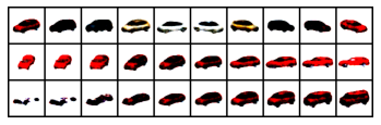
(b) cars3d.

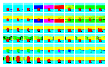
(c) shapes3d.

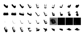
(d) smallnorb.

Figure 6: idvae latent traversals. Each row corresponds to a dimension of $\mathbf{z}$, that we vary in the range $[-3,3]$. We can see that, in some cases, changing a dimension can affect multiple ground-truth factors, meaning that idvae has not obtained full disentanglement. (a) From top to bottom: orientation, scale, shape(?), posY, posX. (b) From top to bottom: azimuth, elevation, object type. (c) From top to bottom: wall color, floor color, object type, azimuth, object color, object size. (d) azimuth, elevation, lighting, category.

Latent traversal is a simple approach to visualize disentangled representations, by plotting the effects that each latent dimension of a randomly selected sample has on the reconstructed output. In fig. 6(a), we evaluate a configuration (single seed) of our idvae model trained on dsprites (other datasets in Appendix F). Every row of the figure represents a latent dimension that we vary in the range $[-3,3]$, while keeping the other dimensions fixed. We can see that $z_{1}$ has learned orientation reasonably well; $z_{2}$ is responsible of the object scale; $z_{4}$ and $z_{5}$ reflect changes on the vertical and horizontal axis, respectively. $z_{3}$ tried to learn, without success, shape changes. Next, we rely on disentanglement metrics to make a quantitative comparison among the tested methods.

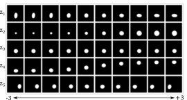
Figure 2: Latent traversal of idvae model trained on dsprites.

Figure 3: Beta score and explicitness (the higher the better). 1=$\beta$-vae, 2=ss-idvae (1%), 3=ss-idvae (10%), 4=idvae, 5=ss-ivae (1%), 6=ss-ivae (10%), 7=ivae, 8=ss-fullvae (1%), 9=ss-fullvae (10%), 10=fullvae. Percentage of labeled samples in parenthesis.

Figure 4: Beta score and explicitness median (the higher the better) as a function of the regularization strength.

Disentanglement Evaluation.

In fig. 3, we report, for each method and for each dataset, the ranges of the beta score and explicitness values with a box-plot. The variance of the box-plots is due to the random seeds and regularization strengths, which are the only parameters we vary. Furthermore, fig. 3 includes the results for ss-idvae, ss-ivae and ss-fullvae (trained with 1% and 10% labeled samples), with different shades of green, blue, and red, respectively. The remaining evaluation metrics can be found in Appendix F, but they are essentially all correlated, as also noted in Locatello et al. (2019).

Overall, we observe, as expected, that $\beta$-vae is often the worst method. Indeed, it has no access to any additional information at training time except the data itself. Despite this, $\beta$-vae disentanglement performance is surprisingly not that far from fullvae that directly matches the latent space with the ground-truth factors. In some cases, $\beta$-vae obtains very high beta scores (see outliers), such as for dsprites and cars3d datasets, confirming the sensitivity to random initialization of unsupervised methods (Locatello et al., 2019). Note also that fullvae exhibits inconsistent performance across the four datasets.

idvae emerges as the best method across several disentanglement metrics, except for smallnorb, where fullvae’s beta score is slightly better. For this specific dataset and metric, there are no considerable differences among methods, since most of the box-plots overlap. We note that idvae outperforms ivae: considering that the two methods differ for the way the conditional prior is learned, our experiments show that an optimal conditional prior, as we propose in this work, offers substantial benefits in terms of disentanglement and it is the only reason for idvae superiority. Finally, although both ivae and idvae have theoretical guarantees on disentanglement and use the full set of ground-truth factors as input, they do not always obtain the maximum evaluation score, in practice. This is in line with the considerations in section 4.1.

The analysis above remains valid if we consider the semi-supervised versions of the tested methods, too. We observe that, with the exception of smallnorb, ss-idvae’s disentanglement performance coherently increases when it observes more labeled instances. The same trend is generally followed by ss-ivae. ss-fullvae, instead, seems to be less susceptible to the number of labeled instances. In general, even a small percentage of labeled instances (1%) is enough for ss-idvae to outperform $\beta$-vae and to keep up with fullvae that is, however, a fully supervised method. This suggests that ss-idvae is a valid choice for applications where collecting additional information about the training data is difficult or expensive.

Impact of the regularization strength.

The disentanglement performance of each method might change drastically as a function of the regularization strength: some approaches might work significantly better in some ranges and very badly in others. In fig. 4, we plot, for each method and for each dataset, the median of the beta score and explicitness evaluation values as a function of the regularization strength. This is also useful to see if there are methods that consistently dominate others. In this case, we do not report the results for ss-idvae, ss-ivae, and ss-fullvae to make the plots more easily readable. Additional disentanglement score results, including the semi-supervised versions, can be found in appendix F.

Across all the datasets, idvae achieves the best median scores for a wide range of regularization strengths. In dsprites, cars3d, and shapes3d, ivae dominates all the other methods (idvae is largely dominant also considering the remaining evaluations metrics). The performance of ivae and fullvae can match that of idvae in some datasets, but the behavior is not consistent: if we focus on beta score, ivae is the second best method in cars3d and shapes3d, whereas in dsprites and smallnorb, performance drops when we increase the regularization strength – even $\beta$-vae performs better; fullvae behaves well for dsprites and smallnorb, but it is on pair only with $\beta$-vae in cars3d and shapes3d.

By observing the evolution of the disentanglement scores, it appears that there is no clear strategy to choose the regularization strength. For idvae, in datasets such as dsprites and cars3d, the regularization strength does not significantly affect the beta score; in shapes3d and smallnorb, we note instead a decreasing monotonic trend. The situation is similar if we look at the explicitness, but it differs if we consider different disentanglement metrics. It is plausible to deduce that the regularization strength is both model and data specific, and it is also affected by the choice of the disentanglement metric.

5.3 Limitations

In our experimental campaign we use the same convolutional architecture for all the methods we compare. We do not vary the optimization hyper-parameters and the dimension of the latent variables. Hence, we cannot ensure that every method runs in its best conditions. Nevertheless, our experimental protocol makes our analysis independent of method-specific optimizations, and has the benefit of reducing training times.

Also, we use the whole set of ground-truth factors as auxiliary variables, in the semi-supervised settings too, whereas it is possible to study the impact of only a subset of the factors to be available. Moreover, idvae and ivae can use any kind of auxiliary variables, as long as they are informative about the ground-truth factors: they are not restricted to using, e.g., labels corresponding to input data, as we (and many other studies) do in our experiments.

Finally, we do not study the implications and benefits of disentanglement for solving complex downstream tasks, which is an interesting task that we leave for future work.

6 Conclusion

In this work, we made a step further in the design of identifiable generative models to learn disentangled representations. idvae uses a prior that encodes ground-truth factor information captured by auxiliary observed variables. The key idea was to learn an optimal representation of the latent space, defined by an inference network on the posterior of the latent variables, given the auxiliary variables. Such posterior is then used as a prior on the latent variables of a second generative model, whose inference network learns a mapping between input observations and latents. We also proposed a semi-supervised version of idvae that can be applied when auxiliary variables are available for a subset of the input observations only. Experimental results offer evidence that idvae and ss-idvae often outperforms existing alternatives to learn disentangled representations, according to several established metrics.

Appendix A ELBO derivation for idvae

$$\log p(\mathbf{x},\mathbf{u}) =log\int p(\mathbf{x},\mathbf{u},\mathbf{z})d\mathbf{z}=$$

$$=log\int p(\mathbf{x}|\mathbf{u},\mathbf{z})p(\mathbf{z}|\mathbf{u})p(\mathbf{u})d\mathbf{z}=$$

$$=log\int\frac{p(\mathbf{x}|\mathbf{u},\mathbf{z})p(\mathbf{z}|\mathbf{u})p(\mathbf{u})}{q(\mathbf{z}|\mathbf{x},\mathbf{u})}q(\mathbf{z}|\mathbf{x},\mathbf{u})d\mathbf{z}\geq\mathcal{L}_{\textrm{{{idvae}}}}$$

$$\geq\mathbb{E}_{q(\mathbf{z}|\mathbf{x},\mathbf{u})}[\log\frac{p(\mathbf{x}|\mathbf{u},\mathbf{z})p(\mathbf{z}|\mathbf{u})p(\mathbf{u})}{q(\mathbf{z}|\mathbf{x},\mathbf{u})}]=$$

$$=\mathbb{E}_{q(\mathbf{z}|\mathbf{x},\mathbf{u})}[\log p(\mathbf{x}|\mathbf{u},\mathbf{z})]-KL(q(\mathbf{z}|\mathbf{x},\mathbf{u})||p(\mathbf{z}|\mathbf{u}))+\log p(\mathbf{u}),$$ (21)

where:

$$\log p(\mathbf{u}) =log\int p(\mathbf{u},\mathbf{z})d\mathbf{z}\geq\mathcal{L}_{\textrm{prior}}=$$

$$=\mathbb{E}_{q(\mathbf{z}|\mathbf{u})}[\log p(\mathbf{u}|\mathbf{z})]-KL(q(\mathbf{z}|\mathbf{u})||p(\mathbf{z})).$$ (22)

Appendix B ELBO derivation for ss-idvae

$$\log p(\mathbf{x}) =log\int p(\mathbf{x},\mathbf{u},\mathbf{z})d\mathbf{u}d\mathbf{z}=$$

$$=log\int p(\mathbf{x}|\mathbf{u},\mathbf{z})p(\mathbf{z}|\mathbf{u})p(\mathbf{u})d\mathbf{u}d\mathbf{z}=$$

$$=log\int\frac{p(\mathbf{x}|\mathbf{u},\mathbf{z})p(\mathbf{z}|\mathbf{u})p(\mathbf{u})}{q(\mathbf{u},\mathbf{z}|\mathbf{x})}q(\mathbf{u},\mathbf{z}|\mathbf{x})d\mathbf{u}d\mathbf{z}\geq$$

$$\geq\mathbb{E}_{q(\mathbf{u},\mathbf{z}|\mathbf{x})}[\log\frac{p(\mathbf{x}|\mathbf{u},\mathbf{z})p(\mathbf{z}|\mathbf{u})p(\mathbf{u})}{q(\mathbf{u},\mathbf{z}|\mathbf{x})}]=$$

$$=\mathbb{E}_{q(\mathbf{z}|\mathbf{x},\mathbf{u})q(\mathbf{u}|\mathbf{x})}[\log\frac{p(\mathbf{x}|\mathbf{u},\mathbf{z})p(\mathbf{z}|\mathbf{u})p(\mathbf{u})}{q(\mathbf{z}|\mathbf{x},\mathbf{u})q(\mathbf{u}|\mathbf{x})}]=$$

$$=\mathbb{E}_{q(\mathbf{u}|\mathbf{x})}[\mathcal{L}_{\textrm{{{idvae}}}}]+\mathcal{H}(q(\mathbf{u}|\mathbf{x})).$$ (23)

Combining eqs. 21, 22 and 23 we obtain $\mathcal{L}_{{\textsc{ss-idvae}}}$, where it is clear that we use the sum over the data samples instead of the expectation. As stated in the main paper, we also add the term – $\mathbb{E}_{(\mathbf{x},\mathbf{u})\sim p_{l}}[\log q(\mathbf{u}|\mathbf{x})]$ – such that it can learn also from labeled data.

Appendix C Sketch of the proof of Theorem 1

In this section, we report a sketch of the proof of Theorem 1. Following the proof strategy of Khemakhem et al. (2020), the proof consists of three main steps.

In the first step, we use assumption (i) to demonstrate that observed data distributions are equal to noiseless distributions. Supposing to have two sets of parameters $(\mathbf{f},\mathbf{T},\boldsymbol{\eta})$ and $(\tilde{\mathbf{f}},\tilde{\mathbf{T}},\tilde{\boldsymbol{\eta}})$, with a change of variable $\bar{\mathbf{x}}=\mathbf{f}(\mathbf{z})=\tilde{\mathbf{f}}(\mathbf{z})$, we show that:

$$\tilde{p}_{\mathbf{T},\boldsymbol{\eta},\mathbf{f},\mathbf{u}}(\mathbf{x})=\tilde{p}_{\tilde{\mathbf{T}},\tilde{\boldsymbol{\eta}},\tilde{\mathbf{f}},\tilde{\mathbf{u}}}(\mathbf{x}),$$ (24)

where:

$$\tilde{p}_{\mathbf{T},\boldsymbol{\eta},\mathbf{f},\mathbf{u}}(\mathbf{x}) =p_{\mathbf{T},\boldsymbol{\eta}}(\mathbf{f}^{-1}(\mathbf{x})|\mathbf{u})|detJ_{\mathbf{f}^{-1}}(\mathbf{x})|\mathbbm{1}_{\mathcal{X}}(\mathbf{x})$$ (25)

In the second step, we use assumption (iv) to remove all the terms that are a function of $\mathbf{x}$ or $\mathbf{u}$. By substituting $p_{\mathbf{T},\boldsymbol{\eta}}$ with its exponential conditionally factorial form, taking the log of both sides of eq. 25, we obtain $dk+1$ equations. Then:

$$\mathbf{T}(\mathbf{f}^{-1}(\mathbf{x}))=\mathbf{A}\mathbf{T}^{\prime}(\mathbf{f}^{\prime-1}(\mathbf{x}))+\mathbf{c}.$$ (26)

In the last step, assumptions (i) and (iii) are used to show that the linear transformation is invertible and so $(\mathbf{f},\mathbf{T},\boldsymbol{\eta})\sim(\tilde{\mathbf{f}},\tilde{\mathbf{T}},\tilde{\boldsymbol{\eta}})$. This concludes the proof.

For a full derivation of the proof, we point the reader to section $\mathbf{B}$ of the supplement in Khemakhem et al. (2020), which holds also for our variant of the theorem.

Appendix D Model architectures, parameters and hyperparameters

All the selected methods (including the semi-supervised variants) share the same convolutional architecture. The conditional prior in ivae is a mlp network, in idvae we use a simple mlp vae, both with leaky ReLU activation functions. The ground-truth factor learner implementing $q_{\boldsymbol{\zeta}}(\mathbf{u}|\mathbf{x})$ in ss-idvae and ss-ivae is a convolutional neural network.

Encoder	Decoder
Input: $64\times 64\times$ number of channels	Input: $\mathbb{R}^{d}$, where $d$ is the number of ground-truth factors
$4\times 4$ conv, 32 ReLU, stride 2	FC, 256 ReLU
$4\times 4$ conv, 32 ReLU, stride 2	FC, $4\times 4\times 64$ ReLU
$4\times 4$ conv, 64 ReLU, stride 2	$4\times 4$ upconv, 64 ReLU, stride 2
$4\times 4$ conv, 64 ReLU, stride 2	$4\times 4$ upconv, 32 ReLU, stride 2
FC 256*, FC $2\times d$	$4\times 4$ upconv, 32 ReLU, stride 2
	$4\times 4$ upconv, number of channels, stride 2

Table 2: Main Encoder-Decoder architecture. In ivae and idvae, we give $\mathbf{u}$ as input to the fully connected layer of the Encoder which size becomes $256+d$.

Conditional Prior Encoder	Conditional Prior Decoder
FC, 1000 leaky ReLU	FC, 1000 leaky ReLU
FC, 1000 leaky ReLU	FC, 1000 leaky ReLU
FC, 1000 leaky ReLU	FC, 1000 leaky ReLU
FC $2\times d$	FC $d$

Table 3: idvae Conditional Prior Encoder-Decoder architecture. ivae uses the encoder only.

Ground-truth Factor Learner
Input: $64\times 64\times$ number of channels. $d$ is the number of ground-truth factors.
$4\times 4$ conv, 32 ReLU, stride 2
$4\times 4$ conv, 32 ReLU, stride 2
$4\times 4$ conv, 64 ReLU, stride 2
$4\times 4$ conv, 64 ReLU, stride 2
FC 256, FC $2\times d$

Table 4: Ground-truth factor learner implementing $q_{\boldsymbol{\zeta}}(\mathbf{u}|\mathbf{x})$ in ss-idvae and ss-ivae.

Parameters	Values
batch_size	64
optimizer	Adam
Adam: beta1	0.9
Adam: beta2	0.999
Adam: epsilon	1e-8
Adam: learning_rate	1e-4
training_steps	300’000

Table 5: Common hyperparameters to each of the considered methods.

Appendix E Implementation of disentanglement metrics

Beta score

The idea behind the beta score (Higgins et al., 2017) is to fix a random ground-truth factor and sample two mini batches of observations from the corresponding generative model. The encoder is then used to obtain a learned representation from the observations (with a ground-truth factor in common). The dimension-wise absolute difference between the two representation is computed and a simple linear classifier $C$ is used to predict the corresponding ground-truth factor. This is repeated $batch\_size$ times and the accuracy of the predictor is the disentanglement metric score.

MIG - Mutual Information Gap

The mutual information gap (MIG) (Chen et al., 2018) is computed as the average, normalized difference between the highest and second highest mutual information of each ground-truth factor with the dimensions of the learned representation. As done in Locatello et al. (2019), we consider the mean representation. and compute the discrete mutual information by binning each dimension of the mean learned representation into $n\_bins$ bins.

Modularity and Explicitness

A representation is modular if each dimension depends on at most one ground-truth factor. Ridgeway & Mozer (2018) propose to measure the Modularity as the average normalized squared difference of the mutual information of the factor of variations with the highest and second-highest mutual information with a dimension of the learned representation. A representation is explicit if it is easy to predict a factor of variation. To compute the explicitness, they train a one-versus-rest logistic regression classifier to predict the ground-truth factor of variation and measeure its ROC-AUC. In the current implementation, observations are discretized into $n\_bins$ bins.

SAP - Separated Attribute Predictability

According to Kumar et al. (2018), the Separated Attribute Predictability (SAP) score is computed from a score matrix where each entry is the linear regression or classification score (in case of discrete factors) of predicting a given ground-truth factors with a given dimension of the learned representation. The (SAP) score is the average difference of the prediction error of the two most predictive learned dimensions for each factor. As done in (Locatello et al., 2019), we use a linear svm as classifier.

As explained in the main paper, the implementation of the selected disentanglement evaluation metrics is based on Locatello et al. (2019). We report the main parameters in table 6.

Disentanglement metrics	Parameters
Beta score	train_size=10’000, test_size=5’000, batch_size=64, predictor=logistic_regression
MIG	train_size=10’000, n_bins=20
Modularity and Explicitness	train_size=10’000, test_size=5’000, batch_size=16, n_bins=20
SAP score	train_size=10’000, test_size=5’000, batch_size=16, predictor=linear svm, C=0.01

Table 6: Disentanglement metrics and their parameters.

Appendix F Full experiments

In this section, we report the full set of experiments, including reconstructions and latent traversals.

(a) dsprites: original observations.

(b) dsprites: reconstructions by idvae.

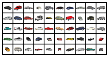
(c) cars3d: original observations.

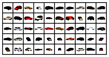
(d) cars3d: reconstructions by idvae.

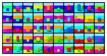
(e) shapes3d: original observations.

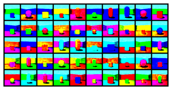
(f) shapes3d: reconstructions by idvae.

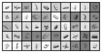
(g) smallnorb: original observations.

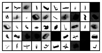
(h) smallnorb: reconstructions by idvae.

Figure 5: Original observations vs idvae reconstructions.

(a) dsprites.

Figure 7: Beta score, MIG, Modularity, Explicitness, and SAP (the higher the better). 1=$\beta$-vae, 2=ss-idvae (1%), 3=ss-idvae (10%), 4=idvae, 5=ss-ivae (1%), 6=ss-ivae (10%), 7=ivae, 8=ss-fullvae (1%), 9=ss-fullvae (10%), 10=fullvae. Percentage of labeled samples in parenthesis.

Figure 8: Beta score, MIG, modularity, explicitness and SAP median (the higher the better) as a function of the regularization strength, for each method on dsprites, cars3d, shapes3d, smallnorb.

References

- Achille & Soatto (2016) Achille, A. and Soatto, S. Information dropout: learning optimal representations through noise. IEEE Trans. Pattern Anal. Mach. Intell., 2016.
- Bengio et al. (2013) Bengio, Y., Courville, A., and Vincent, P. Representation learning: A review and new perspectives. IEEE Trans. Pattern Anal. Mach. Intell., 2013.
- Bishop (2006) Bishop, C. M. Pattern Recognition and Machine Learning (Information Science and Statistics). Springer-Verlag, 2006.
- Bouchacourt et al. (2018) Bouchacourt, D., Tomioka, R., and Nowozin, S. Multi-level variational autoencoder: Learning disentangled representations from grouped observations. In Proc. of the 32nd AAAI Conf. on Artif. Intel., AAAI, 2018.
- Burgess et al. (2017) Burgess, C. P., Higgins, I., Pal, A., Matthey, L., Watters, N., Desjardins, G., and Lerchner, A. Understanding disentangling in -vae. In Proc. of the 30th Int. Conf. on Neural Inf. Proc. Sys., NeurIPS, 2017.
- Chen & Batmanghelich (2020a) Chen, J. and Batmanghelich, K. Weakly supervised disentanglement by pairwise similarities. In Proc. of the 34th AAAI Conf. on Artif. Intel., AAAI, 2020a.
- Chen & Batmanghelich (2020b) Chen, J. and Batmanghelich, K. Robust ordinal vae: Employing noisy pairwise comparisons for disentanglement. ArXiv, 2020b.
- Chen et al. (2018) Chen, T. Q., Li, X., Grosse, R. B., and Duvenaud, D. K. Isolating sources of disentanglement in variational autoencoders. In Proc. of the 31st Int. Conf. on Neural Inf. Proc. Sys., NeurIPS, 2018.
- Cheung et al. (2015) Cheung, B., Livezey, J. A., Bansal, A. K., and Olshausen, B. A. Discovering hidden factors of variation in deep networks. In CoRR, 2015.
- Comon (1994) Comon, P. Independent component analysis, a new concept? Signal Process., 36:287–314, 1994.
- Higgins et al. (2017) Higgins, I., Matthey, L., Pal, A., Burgess, C., Glorot, X., Botvinick, M. M., Mohamed, S., and Lerchner, A. beta-vae: Learning basic visual concepts with a constrained variational framework. In Proc. of the 5th Int. Conf. on Learn. Repr., ICLR, 2017.
- Hoffman & Johnson (2016) Hoffman, M. D. and Johnson, M. J. Elbo surgery: yet another way to carve up the variational evidence lower bound. In Workshop in Adv. in Approx. Bayes. Infer., NeurIPS, 2016.
- Hosoya (2019) Hosoya, H. Group-based learning of disentangled representations with generalizability for novel contents. In Proc. of the 28th Int. Joint Conf. on Artif. Intel., IJCAI, 2019.
- Hyvärinen & Pajunen (1999) Hyvärinen, A. and Pajunen, P. Nonlinear independent component analysis: Existence and uniqueness results. Neural networks, 12:429–439, 1999.
- Khemakhem et al. (2020) Khemakhem, I., Kingma., D. P., Mont, R. P., and Hyvärinen, A. Variational autoencoders and nonlinear ica: A unifying framework. In Proc. of the 23rd Int. Conf. on Artif. Intel. and Stat., AISTATS, 2020.
- Kim & Mnih (2018) Kim, H. and Mnih, A. Disentangling by factorising. In Proc. of the 35th Int. Conf. on Mach. Learn., ICML, 2018.
- Kingma & Welling (2014) Kingma, D. P. and Welling, M. Auto-encoding variational bayes. In Proc. of the 2nd Int. Conf. on Learn. Repr., ICLR, 2014.
- Kingma et al. (2014) Kingma, D. P., Mohamed, S., Rezende, D. J., and Welling, M. Semi-supervised learning with deep generative models. In Proc. of the 27th Int. Conf. on Neural Inf. Proc. Sys., NeurIPS, 2014.
- Klys et al. (2018) Klys, J., Snell, J., and Zemel, R. Learning latent subspaces in variational autoencoders. In Proc. of the 31st Int. Conf. on Neural Inf. Proc. Sys., NeurIPS, 2018.
- Kumar & Poole (2020) Kumar, A. and Poole, B. On implicit regularization in -VAEs. In Proceedings of the 37th International Conference on Machine Learning, ICML, 2020.
- Kumar et al. (2018) Kumar, A., Sattigeri, P., and Balakrishnan, A. Variational inference of disentangled latent concepts from unlabeled observations. In Proc. of the 6th Int. Conf. on Learn. Repr., ICLR, 2018.
- LeCun et al. (2004) LeCun, Y., Huang, F. J., and Bottou, L. Learning methods for generic object recognition with invariance to pose and lighting. In Proc. of the 2004 IEEE Comput. Society Conf. on Comput. Vision and Pat. Recogn., CVPR, 2004.
- Locatello et al. (2019) Locatello, F., Bauer, S., Lucic, M., Gelly, S., Schölkopf, B., and Bachem, O. Challenging common assumptions in the unsupervised learning of disentangled representations. In Proc. of the 36th Int. Conf. on Mach. Learn., ICML, 2019.
- Locatello et al. (2020a) Locatello, F., Poole, B., Rätsch, G., Schölkopf, B., Bachem, O., and Tschannen, M. Weakly-supervised disentanglement without compromises. In Proc. of the 37th Int. Conf. on Mach. Learn., ICML, 2020a.
- Locatello et al. (2020b) Locatello, F., Tschannen, M., Bauer, S., Rätsch, G., Schölkopf, B., and Bachem, O. Disentangling factors of variation using few labels. In Proc. of the 8th Int. Conf. on Learn. Repr., ICLR, 2020b.
- Makhzani & Frey (2017) Makhzani, A. and Frey, B. J. Pixelgan autoencoders. In Proc. of the 30th Int. Conf. on Neural Inf. Proc. Sys., NeurIPS, 2017.
- Mathieu et al. (2019) Mathieu, E., Rainforth, T., Siddharth, N., and Teh, Y. W. Disentangling disentanglement in variational autoencoders. In Proceedings of the 36th International Conference on Machine Learning, ICML, 2019.
- Paszke et al. (2019) Paszke, A., Gross, S., Massa, F., Lerer, A., Bradbury, J., Chanan, G., Killeen, T., Lin, Z., Gimelshein, N., Antiga, L., Desmaison, A., Kopf, A., Yang, E., DeVito, Z., Raison, M., Tejani, A., Chilamkurthy, S., Steiner, B., Fang, L., Bai, J., and Chintala, S. Pytorch: An imperative style, high-performance deep learning library. In Proc. of the 32nd Int. Conf. on Neural Inf. Proc. Sys., NeurIPS. 2019.
- Reed et al. (2015) Reed, S. E., Zhang, Y., Zhang, Y., and Lee, H. Deep visual analogy-making. In Proc. of the 28th Int. Conf. on Neural Inf. Proc. Sys., NeurIPS. Curran Associates, Inc., 2015.
- Rezende et al. (2014) Rezende, D. J., Mohamed, S., and Wiestra, D. Stochastic backpropagation and approximate inference in deep generative models. In Proc. of the 31st Int. Conf. on Mach. Learn., ICML, 2014.
- Ridgeway & Mozer (2018) Ridgeway, K. and Mozer, M. C. Learning deep disentangled embeddings with the f-statistic loss. In Proc. of the 31st Int. Conf. on Neural Inf. Proc. Sys., NeurIPS, 2018.
- Shu et al. (2020) Shu, R., Chen, Y., Kumar, A., Ermon, S., and Poole, B. Weakly supervised disentanglement with guarantees. In Proc. of the 8th Int. Conf. on Learn. Repr., ICLR, 2020.
- Siddharth et al. (2017) Siddharth, N., Paige, B., van de Meent, J., Desmaison, A., Goodman, N., Kohli, P., Wood, F., and Torr, P. Learning disentangled representations with semi-supervised deep generative models. In Proc. of the 30th Int. Conf. on Neural Inf. Proc. Sys., NeurIPS, 2017.
- Tishby et al. (1999) Tishby, N., Pereira, F. C., and Bialek, W. The information bottleneck method. In Proc. of the 34th Annual Allert. Conf. on Comm. Contr and Comput., 1999.
- Titsias & Lázaro-Gredilla (2014) Titsias, M. and Lázaro-Gredilla, M. Doubly stochastic variational bayes for non-conjugate inference. In Proc. of the 31st Int. Conf. on Mach. Learn., ICML, 2014.
- Zhao et al. (2019) Zhao, S., Song, J., and Ermon, S. Infovae: Balancing learning and inference in variational autoencoders. In Proc. of the 33rd AAAI Conf. on Artif. Intel., AAAI, 2019.