anomaly : Detection of Anomalous Structure in Time Series Data

Alex Fisch, Daniel Grose, Idris A. Eckley, Paul Fearnhead, Lawrence Bardwell anomaly : Detection of Anomalous Structure in Time Series Data Detection of Anomalous Structure in Time Series Data One of the contemporary challenges in anomaly detection is the ability to detect, and differentiate between, both point and collective anomalies within a data sequence or time series. The anomaly package has been developed to provide users with a choice of anomaly detection methods and, in particular, provides an implementation of the recently proposed Collective And Point Anomaly family of anomaly detection algorithms. This article describes the methods implemented whilst also highlighting their application to simulated data as well as real data examples contained in the package. anomaly detection, point anomaly, collective anomaly, BARD, CAPA, PASS Daniel Grose
Department of Mathematics and Statistics
Fylde College
Lancaster University
LA1 4YF
United Kingdom
E-mail:
URL: https://www.lancaster.ac.uk/sci-tech/about-us/people/daniel-grose

1 Introduction

Within this article, we focus on the challenge of detecting anomalies within data sequences. Anomaly detection has become an increasingly important area of research activity due to its wide ranging application: from fault detection (theissler2017detecting; zhao2018anomaly), to fraud prevention (ahmed2016survey), and system monitoring (goh2017anomaly). In broad terms, anomalies are observations that do not conform with the general or local pattern of the data and are commonly considered to fall into one of three categories: global anomalies, contextual anomalies, or collective anomalies (nchandolaanomaly-detection-overview). Global anomalies and contextual anomalies are defined as single observations that are outliers with regards to the complete dataset and their local context respectively. Conversely, collective anomalies are defined as sequences of observations that are not anomalous when considered individually, but together form an anomalous pattern (2018arXiv180601947F).

In parallel with the methodological development of statistical anomaly detection for data sequences, a number of software implementations have been developed. For example, within R, the anomalize package (anomalize-package) provides an implementation of two point anomaly approaches, based on the interquartile range and generalized extreme studentized deviate test respectively, following the removal of any seasonal and trend components. Similarly otsad (otsad-package) also provides a suite of approaches for the detection of point anomalies, whilst cbar (cbar-package) seeks to identify contextual anomalies using a Bayesian framework. Conversely, tsoutliers (tsoutliers-package) seeks to detect innovative and additive outliers together within time series, whilst oddstream (oddstream-package) implements an algorithm for the detection of anomalous series within newly arrived collections of series and stray (stray-package) implements the HDoutliers algorithm for various settings including the detection of anomalies in high-dimensional data. Whilst the aforementioned packages arguably represent the current state of the statistical art at the time of writing, a number of other contributions have been made by researchers in other disciplines: see for example Python packages including anomatools (anomatools-package), adtk (adtk-package) and PySAD pysad-package, and Julia contributions including MultivariateAnomalies (esd-8-677-2017) and AnomalyDetection (anomalydetection-package-julia).

This paper describes the anomaly package (anomaly-package) that implements a number of recently proposed methods for anomaly detection. For univariate data there is the Collective And Point Anomaly detection (CAPA) method of 2018arXiv180601947F, that can detect both collective and point anomalies. For multivariate data there are three methods, a multivariate extension of CAPA (2019arXiv190901691F), the Proportion Adaptive Segment Selection (PASS) method of 10.1093-biomet-ass059, and a Bayesian approach, Bayesian Abnormal Region Detector (bardwell2017).

The multivariate CAPA method and PASS are similar in that, for a given segment they use a likelihood-based approach to measure the evidence that it is anomalous for each component of the multivariate data stream, and then merge this evidence across components. They differ in how they merge this evidence, with PASS using higher criticism (donoho2004) and CAPA using a penalised likelihood approach. One disadvantage of the higher criticism approach for merging evidence is that it can lose power when only one or a very small number of components are anomalous. Furthermore, CAPA also allows for point anomalies in otherwise normal segments of data, and can be more robust to detecting collective anomalies when there are point anomalies in the data. CAPA can also allow for the anomalies segments to be slightly mis-aligned across different components.

The BARD method considers a similar model to that of CAPA or PASS, but is Bayesian and so its basic output are samples from the posterior distribution for where the collective anomalies are, and which components are anomalous. It does not allow for point anomalies. As with any Bayesian method, it requires the user to specify suitable priors, but the output is more flexible, and can more directly allow for quantifying uncertainty about the anomalies.

The article begins by providing a brief introduction to anomaly detection before proceeding to give a detailed treatment of each approach. In each case, the relevant methodology is introduced, describing the associated package functionality where appropriate. The methods are applied to a number of test datasets that are available with the package. These data sets comprise the machine temperature data introduced by DBLP:journals/corr/LavinA15, and a microarray genomics dataset. The examples also include details of how the effects of autocorrelation can be accounted for through the adjustment of the method parameters or by applying transforms to preprocess the data prior to analysis.

2 Background

The suite of methods described in this article focuses on collective anomalies. Informally, collective anomalies are segments of data which are anomalous when compared against the general structure of the full data. The modelling paradigm is to assume that there is a common model for data outside the anomalous regions, for example that it is independent normally distributed with a fixed mean and variance, and that collective anomalies correspond to segments of the data that are inconsistent with this, for example due to having a different mean or variance. One approach to modelling this type of anomaly is via epidemic changepoints – a particular form of changepoints admitting one change away from the typical distribution of the data and one back to it at a later time (2018arXiv180601947F). Formally, in the univariate setting, data, $\{{x}_{t}\}$, are said to follow a parametric epidemic changepoint model if $\{{x}_{t}\}$ obey the parametric model $f(x_{t},{\boldsymbol{\theta}}(t))$ at all times and the parameter ${\boldsymbol{\theta}}(t)$ satisfies

$$\theta(t)=\begin{cases}\theta_{1}&s_{1}<t\leq e_{1},\\ &\vdots\\ \theta_{K}&s_{K}<t\leq e_{K},\\ \theta_{0}&\text{otherwise}.\end{cases}$$ (1)

Here $(s_{1},e_{1}),....,(s_{K},e_{K})$ denote the start and end points of $K$ collective anomalies. The typical (baseline) behaviour of the data sequence is defined by the parameter $\theta_{0}$. Conditionally on the parameter $\theta(t)$, all observations ${x}_{t}$ are assumed to be independent, with relaxations of this assumption being discussed in the following sections.

When extending to the multivariate setting, i.e., a $p$-dimensional multivariate time series, it is common to assume that the series are independent, but that their periods of anomalous behaviour align. The copy number variations data set (2011arXiv1106.4199B) provides a good example of such behaviour. In the absence of a copy number variation, data from different individuals can be assumed to be independent. However, when collective anomalies under the form of copy number variations occur, they typically affect a subset of the test subjects. Under such a model, it is well known that joint analysis can lead to significant improvements in detection power over analysing each component individually (donoho2004). The subset multivariate epidemic changepoint model provides a natural model for this type of behaviour. It assumes that

$$\boldsymbol{\theta}^{(i)}(t)=\begin{cases}\boldsymbol{\theta}^{(i)}_{1}&\text{if}\;s_{1}<t\leq e_{1}\;\text{and}\;i\in\textbf{J}_{1},\\ &\vdots\\ \boldsymbol{\theta}^{(i)}_{K}&\text{if}\;s_{K}<t\leq e_{K}\;\text{and}\;i\in\textbf{J}_{K},\\ \boldsymbol{\theta}^{(i)}_{0}&\text{otherwise},\end{cases}\;\;\;\;\;\;\;\;\ 1\leq i\leq p.$$ (2)

where, again, $K$ is the number of collective anomalies with $(s_{k}$,$e_{k})$ denoting the start and end of the $k$th collective anomaly. The $k$th collective anomaly only affects the subset $J_{k}$ of time-series. If the $i$th time-series is affected by the $k$th collective anomaly, i.e., $i\in J_{k}$ then $\theta_{k}^{(i)}$ denotes its parameter value; with $\theta_{0}^{(i)}$ denoting the parameter governing the typical behaviour of the $i$th time-series.

3 The Collective And Point Anomaly Family

The Collective And Point Anomaly (CAPA) family of algorithms (2018arXiv180601947F; 2019arXiv190901691F) differ from many other anomaly detection methods in that they seek to simultaneously detect and distinguish between both collective and point anomalies. CAPA assumes that the data $\{{\bf x}_{t}\}$ follow the model detailed in (1), when univariate or (2) when multivariate. Point anomalies are incorporated within the model as epidemic changes of length one. When analysing multivariate data, CAPA assumes that the collective anomalies don’t overlap, i.e., that $e_{1}\leq s_{2},...,e_{K-1}\leq s_{K}$, whilst allowing for the alignment of collective anomalies to be imperfect, i.e., allowing the components to leave their typical state and return to it at slightly different times.

Whilst the CAPA procedure can allow for many different models for the data, the current implementation assumes that the data is independent and normally distributed, and that the data has been normalised so that the mean is 0 and variance is 1. Non-anomalous data points are drawn from a normal distribution with a specific mean and variance (that the CAPA algorithm will estimate). Collective anomalies correspond to regions where the mean or mean and variance of the data are different.

CAPA infers the number, $K$, and locations $(s_{1},e_{1}),...,(s_{K},e_{K})$ of collective anomalies as well as the set $O$ of point anomalies by maximising the penalised saving function

$$\sum_{i=1}^{K}\left(S(s_{i},e_{i})-\beta(e_{i}-s_{i})\right)+\sum_{t\in O}\left(S^{\prime}(x_{t})-\beta^{\prime}\right),$$ (3)

with respect to $(s_{1},e_{1}),...,(s_{K},e_{K})$ and $K$, subject to constraints on the maximum and minimum lengths of anomalies (see 2018arXiv180601947F for details). Here the saving statistic, $S(s,e)$, of a putative anomaly with start point, $s$, and end point, $e$, corresponds to the improvement in model fit obtained by modelling the data in segment $(s,e)$ as a collective anomaly. Given this improvement will always be non-negative a penalty, $\beta(e_{i}-s_{i}+1)$, potentially depending on the length of the putative anomaly is used to prevent false positives being flagged. The choice of the penalty is model dependent, and discussed in the following sections. Similarly, $S^{\prime}(x_{t})$ and $\beta^{\prime}$ denote the improvement in model fit by assuming observation, $x_{t}$, is a point anomaly.

CAPA makes some important independence assumptions, and also assumes that the mean and variance of the non-anomalous data is constant. As we see below, it can successfully be applied to situations where these assumptions do not hold. There are two approaches to do so. First we can transform the data so that the assumptions are more reasonable – this could be to remove the effect of common factors that induce dependence across components or applying a filter to remove auto-correlation from the noise. Alternatively we can inflate the default penalties so that we still have good properties if there are no collective anomalies. We give an example of this latter approach for the machine temperature data set below.

CAPA maximises the penalised saving in (3) using an optimal partitioning algorithm (2005ISPL-short). By default, the runtime of CAPA family algorithms scales quadratically in the number of observations. In practice, the computational complexity can be reduced by applying a pruning technique developed by killick-jasa that is used in the changepoint package (killick-jss). It is particularly effective when a large number of anomalies is present – leading to a linear relationship between runtime and data size when the number of anomalies is proportional to the size of the data. Another way to reduce the runtime is to impose a maximum length, $m$, for anomalies, the runtime then scaling linearly in both the number of observations and $m$.

The anomaly package contain a single function, capa, for accessing both the univariate and multivariate methods. It has the following arguments.

• x A numeric matrix with n rows and p columns containing the data which is to be inspected. The time series data classes ts, xts, and zoo are also supported.

• beta A numeric vector of length p, giving the marginal penalties. If beta is missing and p = 1 then beta = 3log(n) when the type is "mean" or "robustmean" and beta = 4log(n) otherwise. If p > 1, type ="meanvar" or type = "mean" and max_lag > 0 it defaults to the penalty regime 2’ described in 2018arXiv180601947F. If p > 1, type = "mean"/"meanvar" and max_lag = 0 it defaults to the pointwise minimum of the penalty regimes 1, 2, and 3 in 2018arXiv180601947F.

• beta_tilde A numeric constant indicating the penalty for adding an additional point anomaly. It defaults to 3log(np), where n and p are the data dimensions.

• type A string indicating which type of deviations from the baseline are considered. Can be "meanvar" for collective anomalies characterised by joint changes in mean and variance (the default), "mean" for collective anomalies characterised by changes in mean only, or "robustmean" (only allowed when p = 1) for collective anomalies characterised by changes in mean only which can be polluted by outliers.

• min_seg_len An integer indicating the minimum length of epidemic changes. It must be at least 2 and defaults to 10.

• max_seg_len An integer indicating the maximum length of epidemic changes. It must be at least min_seg_len and defaults to Inf. The computational cost of the CAPA algortihm can be reduced by decreasing the value of max_seg_len.

• max_lag A non-negative integer indicating the maximum start or end lag. Only useful for multivariate data. Default value is 0.

When the x argument to capa is one dimensional (i.e. a vector or $n\times 1$ array or matrix) the univariate method is used and the max_lag argument is ignored, otherwise, the multivariate method is employed. The capa function returns an S4 object of type capa.class for which the generic methods plot and summary have been provided.

3.1 Univariate CAPA

The anomaly package supports univariate CAPA via the capa function for detecting segments characterised by an anomalous mean or anomalous mean and variance. When investigating segments for an anomalous mean against a typical Gaussian background of mean 0 and variance 1. If we let $f(x;\mu,\sigma)$ denote the density function for a normal random variable with mean $\mu$ and variance $\sigma^{2}$ evaluated at $x$, then the savings for a collective anomaly are equal to the improvement in log-likelihood by fitting a segment as anomalous. When only the mean of an anomalous segment changes,

$$\max_{\mu}\sum_{t=s}^{e}\left\{\log f(x_{t};\mu,1)-\log f(x_{t};0,1)\right\}.$$

While the saving for a point anomaly is set to be the saving for a collective anomaly of length 1. This gives

$$S(s,e)=(e-s+1)\left(\bar{x}_{s:e}\right)^{2}\;\;\;\;\;\;\text{and}\;\;\;\;\;\;S^{\prime}(x)=x^{2}$$

where $\bar{x}_{s:e}$ denotes the mean of observations $x_{s},...,x_{e}$. Conversely, when investigating segments for an anomalous mean and/or variance, savings is

$$\max_{\mu,\sigma}\sum_{t=s}^{e}\left\{\log f(x_{t};\mu,\sigma)-\log f(x_{t};0,1)\right\},$$

with the saving for a point anomaly being that for a change in variance only in a segment of size 1. This gives

$$S(s,e)=\sum_{t=s}^{e}x_{t}^{2}-(e-s+1)\left(1+\log\left(\frac{\sum_{t=s}^{e}\left(x_{t}-\bar{x}_{s:e}\right)^{2}}{e-s+1}\right)\right)\;\;,\;\;S^{\prime}(x)=x^{2}-1-\log\left(e^{-\beta^{\prime}}+x^{2}\right)$$

Note that the data, x, requires standardisation using robust estimates for the typical mean (the median) and the typical variance (the median absolute deviation) obtained on the complete data series so that the above cost functions can be used. See (2019arXiv190901691F) for further details.

The argument max_seg_len sets the maximum length of a collective anomaly. It can be used to prevent the detection of weak but long anomalies which typically arise as a result of model misspecification and also to reduce the run time of the CAPA algorithm. It defaults to a value equal to the length of the data series. Care is needed, as if a value is set that is smaller than the size of the actual anomalous regions, then CAPA is likely to fit multiple collective anomalies to such a region.

By default, $\beta=3\log(n)$ and $\beta=4\log(n)$ are used for changes in mean and changes in mean and variance respectively, and $\beta^{\prime}=3\log n$ for all models, as they have been shown to control the number of false positives when all observations are independent and identically distributed (i.i.d.) Gaussian (2018arXiv180601947F; 2019arXiv190901691F). These default parameters have a tendency to return many false positives on structured, i.e., non independent, data. In this case, beta and beta_tilde should be inflated whilst keeping their ratio constant. When looking for changes in mean, using

$$\beta=\tilde{\beta}=3\frac{1+\hat{\rho}}{1-\hat{\rho}}\log(n),$$ (4)

where $\hat{\rho}$ is a robust estimate for the $AR(1)$-autocorrelation often yields good false positive control. For changes in mean and variance,

$$\beta=4\frac{1+\hat{\rho}}{1-\hat{\rho}}\log(n),~{}~{}\tilde{\beta}=3\frac{1+\hat{\rho}}{1-\hat{\rho}}\log(n).$$

The specific factor is justified theoretically in LavielleMarc2000LEoa.

Alternatively, the data $x_{t}$ can be directly transformed using

$$x_{t}^{\prime}=\sqrt{\frac{1-\hat{\rho}}{1+\hat{\rho}}}\left(\frac{x_{t}-\hat{\mu}}{\hat{\sigma}}\right),$$ (5)

where $\hat{\mu}$ is the median, and $\hat{\sigma}$ is a robust estimator of the standard deviation of the data x, such as based on the inter-quartile range, or the median absolute deviation from the median. This transform should only be used when looking for mean anomalies.

3.1.1 Simulated data

To demonstrate univariate capa a data series of 5000 normally distributed observations with 3 collective anomalies and four point anomalies is analysed. The data can be reproduced using the code provided below, which also runs the analyses and summarises the results. R> library("anomaly") R> set.seed(0) R> x <- rnorm(5000) R> x[401:500] <- rnorm(100, 4, 1) R> x[1601:1800] <- rnorm(200, 0, 0.01) R> x[3201:3500] <- rnorm(300, 0, 10) R> x[c(1000, 2000, 3000, 4000)] <- rnorm(4, 0, 100) R> x <- (x - median(x)) / mad(x) R> res <- capa(x) R> summary(res) Univariate CAPA detecting changes in mean and variance. observations = 5000 minimum segment length = 10 maximum segment length = 5000

Point anomalies detected : 4 location variate strength 1 1000 1 43.07885 2 2000 1 117.84647 3 3000 1 37.49265 4 4000 1 62.67104

Collective anomalies detected : 3 start end variate start.lag end.lag mean.change variance.change 1 401 500 1 0 0 14.597971638 4.990295e-04 2 1601 1800 1 0 0 0.001502774 9.869876e+01 3 3201 3500 1 0 0 0.036926415 7.764414e+00 R> plot(res) The summary method displays information regarding the analysis and details regarding the location and nature of the detected anomalies. The formatting demonstrates that capa correctly determines the presence of the anomalies in the simulated data. The plot function generates a ggplot object (h-wickham-ggplot2-book) which is shown in Figure 1a. The location of the collective anomalies are highlighted by vertical blue bands and the data point anomalies are shown in red.

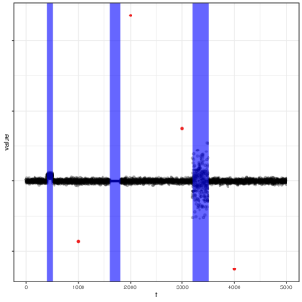
(a)

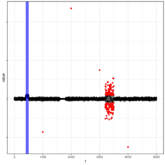
(b)

Figure 1: Visualisation of data, collective and point anomalies detected by CAPA for the simulated univariate data. (a) detecting changes in mean and variance. (b) detecting changes in mean only. The blue regions correspond to the predicted anomalous segments and the red dots indicate point anomalies.

By default, CAPA detects both changes in mean and variance. The option type=”mean” can be used to detect changes in mean only. R> res <- capa(x, type = "mean") R> collective_anomalies(res) start end mean.change test.statistic 1 401 500 14.92774 1492.774 R> head(point_anomalies(res)) location strength 1 1000 43.07885 2 2000 117.84647 3 3000 37.49265 4 3201 11.44038 5 3202 16.52037 6 3203 10.58874 In this case, capa correctly identifies the collective change in mean and the point anomalies. However, as a consequence of CAPA now looking for changes in mean only, and assuming constant variance, the analysis results in changes in variance being classified as groups of point anomalies, see Figure (1b). The above example also demonstrates the collective_anomalies function, which is used to produce a data frame containing the location and change in mean for collective anomalies, and the point_anomalies function which provides the location and strength of the point anomalies.

As previously noted, the CAPA algorithm assumes that the data has been standarised. When this is not the case, false anomalous regions may be identified, as is the case in the following example. R> res <- capa(1 + 2 * x, type = "mean") R> nrow(collective_anomalies(res)) 47

3.1.2 Real data - machine temperature

To demonstrate the application of capa to real univariate data, a data stream from the Numenta Anomaly Benchmark corpus (AHMAD2017134) consisting of temperature sensor data of an internal component of a large industrial machine is analysed. The dataset is included, with permission, in the anomaly package on the condition that derived work be kindly requested to acknowledge (AHMAD2017134).

The machine temperature data consists of 22695 observations recorded at 5 minute intervals and contains three known anomalies as identified by an engineer working on the machine (Figure 2a). The first anomaly corresponds to a planned shutdown of the machine and the third anomaly to a catastrophic failure of the machine. The second anomaly, which can be difficult to detect, corresponds to the onset of a problem which led to the eventual system failure (DBLP:journals/corr/LavinA15). Using capa with default parameters for the (normalised) data results in the detection of $97$ collective anomalies. data("machinetemp") attach(machinetemp) x <- (temperature - median(temperature)) / mad(temperature) res <- capa(x, type = "mean") canoms <- collective_anomalies(res) dim(canoms)[1] [1] 97 One potential source of this over sensitivity is the presence of autocorrelation in the data. A robust estimate for the $AR(1)$-autocorrelation $\hat{\rho}$ can be obtained using the covMcd method from the robustbase package. R> library("robustbase") R> n <- length(x) R> x.lagged <- matrix(c(x[1:(n - 1)], x[2:n]), n - 1, 2) R> rho_hat <- covMcd(x.lagged, cor = TRUE)$cor[1,2]whichgivesanestimatefor$^ρ$of0.987.Asmentionedabove,thedefaultpenaltieshaveatendencytoreturnmanyfalsepositivesonstructured,i.e.,nonindependent,data.Insteadwecaninflatethepenaltiesbasedonourestimatesoftheautocorrelation.R>inflated{}_{p}enalty<-3\ast (1+rho{}_{h}at)/(1-rho{}_{h}at)\ast log(n)R>res<-capa(x,type=\mathrm{"}mean\mathrm{"},beta=inflated{}_{p}enalty,+beta{}_{t}ilde=inflated{}_{p}enalty)R>summary(res)UnivariateCAPAdetectingchangesinmean.observations=22695minimumsegmentlength=10maximumsegmentlength=22695Pointanomaliesdetected:0Collectiveanomaliesdetected:4startendvariatestart.lagend.lagmean.changetest.statistic\mathrm{1161223271009.1489526550.65023773400210025.6488885899.244316023172041008.1917339682.6284191661977510039.42684724050.377}R>plot(res)ThenewpredictedcollectiveanomaliesareshowninFigure\text{<a href="\#S3.F2.sf2" title="In Figure 2 ‣ 3.1.2 Real data - machine temperature ‣ 3.1 Univariate CAPA ‣ 3 The Collective And Point Anomaly Family ‣ pkganomaly : Detection of Anomalous Structure in Time Series Data" class="ltx\_ref ltx\_font\_italic"><span class="ltx\_text ltx\_ref\_tag">2b</span></a>}.Thesecond,thirdandfourthcollectiveanomaliesdetectedusingthemodifiedpenaltyvaluescorrespondwellwiththeknownanomalies.Thefirstanomalyontheotherhanddoesnothaveacorrespondinglabelwhichmeansthatitiseitherafalsepositiveorananomalycorrespondingtoaneventwhichhasnotbeendetectedorrecorded.Notethattheteststatisticforthefirstanomalyisstrongerthanforthesecond,buthassmallerchangeinmean.Thisisinherentinthedefinitionforthevalueoftheteststatisticusedwheninferringchangesinmean,whichisthechangeinmeanmultipliedbythelength(duration)oftheanomaly.\text{Figure 2Figure 22Figure 2(a)2a2aa(a)(b)2b2bb(b)2Timeseriesofmachinetemperatureda}$