Characterizing Deep Gaussian Processes via Nonlinear Recurrence Systems

Abstract

Recent advances in Deep Gaussian Processes (DGPs) show the potential to have more expressive representation than that of traditional Gaussian Processes (GPs). However, there exists a pathology of deep Gaussian processes that their learning capacities reduce significantly when the number of layers increases. In this paper, we present a new analysis in DGPs by studying its corresponding nonlinear dynamic systems to explain the issue. Existing work reports the pathology for the squared exponential kernel function. We extend our investigation to four types of common stationary kernel functions. The recurrence relations between layers are analytically derived, providing a tighter bound and the rate of convergence of the dynamic systems. We demonstrate our finding with a number of experimental results.

1 Introduction

Deep Gaussian Process (DGP) (deep_gp_2013) is a new promising class of models which are constructed by a hierarchical composition of Gaussian processes. The strength of this model lies in its capacity to have richer representation power from the hierarchical construction and its robustness to overfitting from the probabilistic modeling. Therefore, there have been extensive studies (nested_deep_gp; auto_encode_deep_gp; expect_propagation_deep_gp; rff_deep_gp; doubly_deep_gp; hamiltonian_deep_gp; deep_gp_importance_weight; dgp1; dgp2) contributing to this research area.

There exists a pathology, stating that the increase in the number of layers degrades the learning power of DGP (pathology_deep_gp). That is, the functions produced by DGP priors become flat and cannot fit data. It is important to develop theoretical understanding of this behavior, and therefore to have proper tactics in designing model architectures and parameter regularization to prevent the issue. Existing work (pathology_deep_gp) investigates the Jacobian matrix of a given model which can be analytically interpreted as the product of those in each layer. Based on the connection between the manifold of a function and the spectrum of its Jacobian, the authors show the degree of freedom is reduced significantly at deep layers. Another work (how_deep) studies the ergodicity of the Markov chain to explain the pathology.

To explain such phenomena, we study a quantity which measures the distance of any two layer outputs. We present a new approach that makes use of the statistical properties of the quantity passing from one layer to another layer. Therefore, our approach accurately captures the relations of the distance quantity between layers. By considering kernel hyperparameters, our method recursively computes the relations of two consecutive layers. Interestingly, the recurrence relations provide a tighter bound than that of (how_deep) and reveal the rate of convergence to fixed points. Under this unified approach, we further extend our analysis to five popular kernels which are not analyzed yet before. For example, the spectral mixture kernels do not suffer the pathology. We further provide a case study in DGP, showing the connection between our recurrence relations and learning DGPs.

Our contributions in this paper are: (1) we provide a new perspective of the pathology in DGP under the lens of chaos theory; (2) we show that the recurrence relation between layers gives us the rate of convergence to a fixed point; (3) we give a unified approach to form the recurrence relation for several kernel functions including the squared exponential kernel function, the cosine kernel function, the periodic kernel function, the rational quadratic kernel function and the spectral mixture kernel; (4) we justify our findings with numerical experiments. We use the recurrence relations in debugging DGPs and explore a new regularization on kernel hyperparameters to learn zero-mean DGPs.

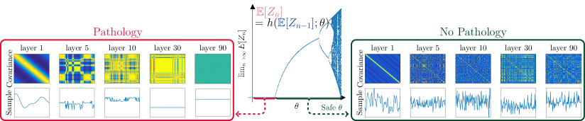
Figure 1: Studying the squared distance, $Z_{n}$, between outputs of two consecutive layers. The asymptotic property (middle plot) of the recurrence relation of this quantity between two consecutive layers decides the existence of pathology for a very deep model. Here, $\theta$ indicates kernel hyperparameters. The middle plot is the bifurcation plot providing the state of DGP at very deep layer. The pathology is identified by the zero-value region where $\mathbb{E}[Z_{n}]\to 0$. Note that this bifurcation plot is for illustration purpose only.

2 Background

Notation   Throughout this paper, we use the boldface as vector or vector-value function. The superscript i.e. $f^{(d)}({\bf{x}})$ is the $d$-th dimension of vector-valued function $\bm{f}({\bf{x}})$.

2.1 Deep Gaussian Processes

We study DGPs in composition formulation where GP layers are stacked hierarchically. An $N$-layer DGP is defined as

$$\bm{f}_{N}\circ\bm{f}_{N-1}\circ\dots\circ\bm{f}_{1}({\bf{x}}),$$

where, at layer $n$, for dimension $d$, $f^{(d)}_{n}|\bm{f}_{n-1}\sim\mathcal{GP}(0,k_{n}(\cdot,\cdot))$ independently. Note that the GP priors have the mean functions set to zero. The nonzero-mean case is discussed later (Section 4.4). We shorthand $\bm{f}_{n}\circ\bm{f}_{n-1}\circ\dots\circ\bm{f}_{1}({\bf{x}})$ as $\bm{f}_{n}({\bf{x}})$ and write $k_{n}(\bm{f}_{n-1}({\bf{x}}),\bm{f}_{n-1}({\bf{x}}^{\prime}))$ as $k_{n}({\bf{x}},{\bf{x}}^{\prime})$. Let $m$ be the number of output of $\bm{f}_{n}$. All layers have the same hyperparameters.

Theorem 2.1 ((how_deep)).

Assume that $k({\bf{x}},{\bf{x}}^{\prime})$ is given by the squared exponential kernel function with variance $\sigma^{2}$ and lengthscale $\ell^{2}$ and that the input ${\bf{x}}$ is bounded. Then if $\sigma^{2}<\ell^{2}/m$,

$$\mathbb{P}(\left\|\bm{f}_{n}({\bf{x}})-\bm{f}_{n}({\bf{x}}^{\prime})\right\|_{2}\xrightarrow[n\to\infty]{}0\quad\text{ for all }{\bf{x}},{\bf{x}}^{\prime}\in\mathcal{D})=1$$

where $\mathbb{P}$ denotes the law of process $\{f_{n}\}$.

This theorem tells us the criterion that the event of vanishing in output magnitude happens infinitely often with probability $1$.

2.2 Analyzing dynamic systems with chaos theory

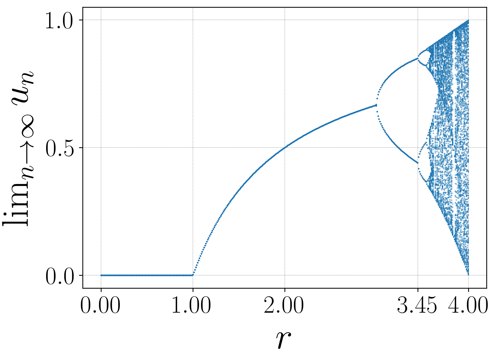
Figure 2: Bifurcation plot of the logistic function $u_{n}=ru_{n-1}(1-u_{n-1})$.

Recurrence maps representing dynamic transitions between DGP layers are nonlinear. Studying the dynamic states and convergence properties for nonlinear recurrences is not as well-established as those of linear recurrences. As an example, given a simple nonlinear model like the logistic map: $u_{n}=ru_{n-1}(1-u_{n-1})$, its dynamic behaviors can be complicated (nature_dynamic).

Recurrent plots or bifurcation plots have been used to analyze the behavior of chaotic systems. The plots are produced by simulating and recording the dynamic states up to very large time points. This tool allows us to monitor the qualitative changes in a system, illustrating fixed points asymptotically, or possible visited values. Other techniques, e.g. transient chaos (transient_chaos_dnn), recurrence relations (deep_information_propagation) have been used to study deep neural networks.

We take the logistic map as an example to understand a recurrence relation. Figure 2 is the bifurcation plot of the logistic map. This logistic map is used to describe the characteristics of a system which models a population function. We can see that the plot reveals the state of the system, showing whether the population becomes extinct ($0<r<1$), stable ($1<r<3$), or fluctuating ($r>3.4$) by seeing the parameter $r$.

3 Moment-generating function of distance quantity

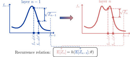
Figure 3: Finding the recurrence relation of the quantity $\mathbb{E}[(f_{n}(x)-f_{n}(x^{\prime}))^{2}]$ between two consecutive layers.

Throughout this paper, we are interested in quantifying the expectation of the squared Euclidean distance between any two outputs of a layer and thereby study the dynamics of this quantity from a layer to the next layer. Figure 1 shows that we can make use of the found recurrence relations to study the pathology of DGPs.

For any input pair ${\bf{x}}$ and ${\bf{x}}^{\prime}$, we define such quantity at layer $n$ as $Z_{n}=\left\|\bm{f}_{n}({\bf{x}})-\bm{f}_{n}({\bf{x}}^{\prime})\right\|_{2}^{2}=\sum_{d=1}^{m}\left(f^{(d)}_{n}({\bf{x}})-f^{(d)}_{n}({\bf{x}}^{\prime})\right)^{2}.$ When the previous layer $\bm{f}_{n-1}$ is given, the difference between any $f^{(d)}_{n}({\bf{x}})$ and $f^{(d)}_{n}({\bf{x}}^{\prime})$ is Gaussian,

$$\left(f^{(d)}_{n}({\bf{x}})-f_{n}^{(d)}({\bf{x}}^{\prime})\right)|\bm{f}_{n-1}\sim\mathcal{N}(0,s_{n}).$$

Here $s_{n}=k_{n}({\bf{x}},{\bf{x}})+k_{n}({\bf{x}}^{\prime},{\bf{x}}^{\prime})-2k_{n}({\bf{x}},{\bf{x}}^{\prime})$ which is obtained from subtracting two dependent Gaussians. We can normalize the difference between $f^{(d)}_{n}({\bf{x}})$ and $f^{(d)}_{n}({\bf{x}}^{\prime})$ by a factor $\sqrt{s_{n}}$ to obtain the form of standard normal distribution as

$$\frac{(f^{(d)}_{n}({\bf{x}})-f^{(d)}_{n}({\bf{x}}^{\prime}))}{\sqrt{s_{n}}}|\bm{f}_{n-1}\sim\mathcal{N}(0,1).$$

Since all dimensions $d$ in a layer are independent, we can say that $\frac{Z_{n}}{s_{n}}|\bm{f}_{n-1}\sim\chi^{2}_{m},$ is distributed according to the Chi-squared distribution with $m$ degrees of freedom.

One useful property of the Chi-squared distribution is that the moment-generating function of $\frac{Z_{n}}{s_{n}}|\bm{f}_{n-1}$ can be written in an analytical form, with $t\leq 1/2$,

$$M_{\frac{Z_{n}}{s_{n}}|\bm{f}_{n-1}}(t)=\mathbb{E}\left[\exp\left(t\frac{Z_{n}}{s_{n}}\right)|\bm{f}_{n-1}\right]=(1-2t)^{-m/2}.$$ (1)

We shall see that the expectation of the distance quantity $Z_{n}$ is computed via a kernel function which, in most cases, involves exponentiations. Given that the input of this kernel is governed by a distribution, i.e., $\chi^{2}$, the moment-generating function becomes convenient to obtain our desired expectations.

Figure 3 depicts our approach to extract a function $h(\cdot)$ which models the recurrence relation between $\mathbb{E}[Z_{n}]$ and $\mathbb{E}[Z_{n-1}]$. This is also the main theme of this paper.

4 Finding recurrence relations

This section presents the formalization of the recurrence relation of $\mathbb{E}[Z_{n}]$ for each kernel function. We start off with the squared exponential kernel function.

4.1 Squared exponential kernel function

The squared exponential kernel () is defined in the form of

$${\lx@acro@@@def{SE}{SE}{}{{SE}}{{}}}({\bf{x}},{\bf{x}}^{\prime})=\sigma^{2}\exp\left(-{\left\|{\bf{x}}-{\bf{x}}^{\prime}\right\|^{2}}/{2\ell^{2}}\right).$$ (2)

Theorem 4.1 (DGP with ).

Given a triplet $(m,\sigma^{2},\ell^{2}),$ $m\geq 1$ such that the following sequence converges to $0$:

$$u_{n}=2m\sigma^{2}\left(1-(1+{u_{n-1}}/{m\ell^{2}})^{-m/2}\right),$$ (3)

Then, $\mathbb{P}(\left\|\bm{f}_{n}({\bf{x}})-\bm{f}_{n}({\bf{x}}^{\prime})\right\|_{2}\xrightarrow[n\to\infty]{}0\text{ for all }{\bf{x}},{\bf{x}}^{\prime}\in\mathcal{D})=1.$

Proof.

Note that we do not directly have access to $\mathbb{E}[Z_{n}]$ but $\mathbb{E}[Z_{n}|\bm{f}_{n-1}]$ because of the Markov structure of the DGP construction. Getting $\mathbb{E}[Z_{n}]$ is done via $\mathbb{E}[Z_{n}|\bm{f}_{n-1}]$ where we use the law of total expectation $\mathbb{E}[Z_{n}]=\mathbb{E}_{\bm{f}_{n-1}}[\mathbb{E}[Z_{n}|\bm{f}_{n-1}]]$.

Now, we study the term $\mathbb{E}[Z_{n}|\bm{f}_{n-1}]$:

$$\mathbb{E}[Z_{n}|\bm{f}_{n-1}]= \mathbb{E}[\sum_{d=1}^{m}(f_{n}^{(d)}(x)-f_{n}^{(d)}(x^{\prime}))^{2}|\bm{f}_{n-1}]$$ (4)

$$= 2m\sigma^{2}-2mk_{n}({\bf{x}},{\bf{x}}^{\prime}).$$

The second equality is followed by $\mathbb{E}[(f^{(d)}_{n}({\bf{x}}))^{2}]={\mathbb{E}[(f_{n}^{(d)}({\bf{x}}^{\prime}))^{2}]}=\sigma^{2}$ and $\mathbb{E}[f_{n}^{(d)}({\bf{x}})f_{n}^{(d)}({\bf{x}}^{\prime})]=k_{n}({\bf{x}},{\bf{x}}^{\prime})$. Recall that we write $k_{n}({\bf{x}},{\bf{x}})=k_{n}(\bm{f}_{n-1}({\bf{x}}),\bm{f}_{n-1}({\bf{x}}^{\prime}))$. By the definition of kernel, we have

$$\mathbb{E}[Z_{n}|\bm{f}_{n-1}] =2m\sigma^{2}\left(1-\exp\left(-\frac{Z_{n-1}}{2\ell^{2}}\right)\right).$$

Applying the law of total expectation, we have

$$\mathbb{E}[Z_{n}]=2m\sigma^{2}\left(1-\mathbb{E}\left[\exp\left(-\frac{Z_{n-1}}{2\ell^{2}}\right)\right]\right).$$

Again, we can only compute $\mathbb{E}[\exp(-\frac{Z_{n-1}}{2\ell^{2}})]=\mathbb{E}_{\bm{f}_{n-2}}[\mathbb{E}[\exp(-\frac{Z_{n-1}}{2\ell^{2}})|\bm{f}_{n-2}]$. The expectation will be computed by the formula of the moment-generating function with respect to $\frac{Z_{n-1}}{s_{n-1}}|\bm{f}_{n-2}$ where $t=-\frac{s_{n-1}}{2\ell^{2}}$ in Equation (1). Choosing this value also satisfies the condition $t\leq 1/2$. Now, we have

$$\mathbb{E}[Z_{n}] =2m\sigma^{2}\left(1-\mathbb{E}\left[\left(1+{s_{n-1}}/{\ell^{2}}\right)^{-m/2}\right]\right)$$ (5)

$$\leq 2m\sigma^{2}\left(1-\left(1+{\mathbb{E}\left[s_{n-1}\right]}/{\ell^{2}}\right)^{-m/2}\right).$$

Here, Jensen’s inequality is used as $(1+x)^{-a}$ is convex for any $x>0$. By Equation (4), we have

$$\frac{\mathbb{E}[Z_{n-1}|\bm{f}_{n-2}]}{m}=2\sigma^{2}-2k_{n-1}({\bf{x}},{\bf{x}}^{\prime})=s_{n-1}.$$

Replacing $s_{n-1}$ in Equation (5) and applying the law of total expectation for the case of $Z_{n-1}$, we obtain recurrence relation between layer $n-1$ and layer $n$ is

$$\mathbb{E}[Z_{n}]\leq 2m\sigma^{2}\left(1-\left(1+{\mathbb{E}[Z_{n-1}]}/{m\ell^{2}}\right)^{-m/2}\right).$$

Using the Markov inequality, for any $\epsilon$, we can bound $\mathbb{P}(Z_{n}\geq\epsilon)\leq\frac{\mathbb{E}[Z_{n}]}{\epsilon^{2}}.$

At this point, $u_{n}$ defined in Equation (3) is considered as the upper bound of $\mathbb{E}[Z_{n}]$. We condition that $\{u_{n}\}$ converges to $0$, then $\{\mathbb{E}[Z_{n}]\}$ converges to $0$ as well. By the first Borel-Cantelli lemma, we have $\mathbb{P}(\limsup_{n\to\infty}{Z_{n}}\geq\epsilon)=0,$ which leads to the conclusion in the same manners as (how_deep). ∎

Figure 4: (a): Bifurcation plot of the recurrence relation of kernel for $m=1$. (b): Contour plot of $u_{n}$ at layer $n=300$ and $m=1$. The misalignment between the red line ($\nicefrac{{\sigma^{2}}}{{\ell^{2}}}=1$) and the zero-level contour is due to numerical errors. (c): Increase $m>\sigma^{2}/\ell^{2}$ to avoid pathology.

Analyzing the recurrence   Figure 4a illustrates the bifurcation plot of Equation (3) with $m=1$. The non-zero contour region in Figure 4b tells us that $\sigma^{2}/\ell^{2}$ should be smaller than $1$ to escape the pathology. When $m>1$, Figure 4c shows that if $m>\sigma^{2}/\ell^{2}$, $u_{n}$ does not approach to $0$, implying the condition to prevent the pathology. This result is consistent with Theorem 2.1 in (how_deep).

Discussion   Note that the relation between $\mathbb{E}[Z_{n}]$ and $\mathbb{E}[Z_{n-1}]$ presents a tighter bound than existing work (how_deep). If we construct the recurrence relation based on (how_deep), $\mathbb{E}[Z_{n}]$ is bounded by

$$\mathbb{E}[Z_{n}]\leq\frac{m\sigma^{2}}{\ell^{2}}\mathbb{E}[Z_{n-1}].$$ (6)

One can show that $(1+x)^{a}\geq 1-ax,a<0,x>0$, implying

$$2m\sigma^{2}(1-(1+\mathbb{E}[Z_{n-1}]/(m\ell^{2}))^{-m/2})\leq m\sigma^{2}\mathbb{E}[Z_{n-1}]/\ell^{2}.$$

In fact, a numerical experiment shows that our bound of $\mathbb{E}[Z_{n}]$ is found to be close to the true $\mathbb{E}[Z_{n}]$ (Section LABEL:sec:correct_recur_relations). That is, we can see the trajectory of $\mathbb{E}[Z_{n}]$ for every layer of a given model of which the depth is not necessary to be infinitely many.

One can reinterpret the recurrence relation for each dimension $d$ as

$$\textstyle{\mathbb{E}[Z_{n}^{(d)}]}\leq 2\sigma^{2}\left(1-\left(1+{\mathbb{E}[Z_{n-1}^{(d)}]}/{\ell^{2}}\right)^{-m/2}\right),$$

where ${\mathbb{E}[Z^{(d)}_{n}]}{=}{\frac{\mathbb{E}[Z_{n}]}{m}}$ with ${Z^{(d)}_{n}}{=}{\left(f^{(d)}_{n}({\bf{x}})-f^{(d)}_{n}({\bf{x}}^{\prime})\right)^{2}}$.

A guideline to obtain a recurrence relation   Given a specific kernel function, one may follow these steps to acquire the corresponding recurrence relation: (1) considering the form of kernel input where it may be distributed according to either the Chi-squared distribution or its variants (presented in the next sections); (2) checking whether there is a way to represent the kernel function under representations such that statistical properties of kernel inputs are known; (3) caring about the convexity of the function after choosing a proper setting (as we bound the expectation with Jensen’s inequality in the proof of Theorem 4.1).

4.2 Cosine kernel function

The cosine kernel () function takes inputs as the distance between two points instead of the squared distance like in the case of kernel. We will mainly work with $\sqrt{Z_{n}}$ in this subsection. The cosine kernel function $k({\bf{x}},{\bf{x}}^{\prime})={\lx@acro@@@def{Cos}{Cos}{}{{Cos}}{{}}}({\bf{x}},{\bf{x}}^{\prime})$ which is defined as

$${\lx@acro@@@def{Cos}{Cos}{}{{Cos}}{{}}}({\bf{x}},{\bf{x}}^{\prime})=\sigma^{2}\cos\left({\pi\left\|{\bf{x}}-{\bf{x}}^{\prime}\right\|_{2}}/{p}\right).$$

Starting with Equation (4) and using the definition of kernel, we have

$$\textstyle\mathbb{E}[Z_{n}|\bm{f}_{n-1}]= 2m\sigma^{2}-2m\sigma^{2}\cos({\pi\sqrt{Z_{n-1}}}/{p})$$

$$= 2m\sigma^{2}-m\sigma^{2}\exp({i\pi\sqrt{Z_{n-1}}}/{p})$$

$$\quad-m\sigma^{2}\exp(-{i\pi\sqrt{Z_{n-1}}}/{p}).$$

Here, Euler’s formula is used to represent $\cos(\cdot)$ and $i$ is the imaginary unit ($i^{2}=-1$). To obtain $\mathbb{E}[Z_{n}]$, we use the law of total expectation and compute the two following expectations: $\mathbb{E}\left[\exp({i\pi\sqrt{Z_{n-1}}}/{p})|\bm{f}_{n-2}\right]$ and $\mathbb{E}\left[\exp(-{i\pi\sqrt{Z_{n-1}}}/{p})|\bm{f}_{n-2}\right]$. From $\frac{Z_{n}}{s_{n}}|\bm{f}_{n-1}\sim\chi^{2}_{m}$, we have $\sqrt{\frac{Z_{n}}{s_{n}}}|\bm{f}_{n-1}\sim\chi_{m},$ is distributed according to the Chi distribution. This observation follows the first step in the guideline. The characteristic function of the Chi distribution for random variable $\sqrt{\frac{Z_{n}}{s_{n}}}|\bm{f}_{n-1}$ is

$$\varphi_{\sqrt{{Z_{n}}/{s_{n}}}|\bm{f}_{n-1}}(t)=\mathbb{E}\left[\exp\left(it\sqrt{{Z_{n}}/{s_{n}}}\right)\right]$$

$$={}_{1}F_{1}(\frac{m}{2},\frac{1}{2},\frac{-t^{2}}{2})+it\sqrt{2}\frac{\Gamma((m+1)/2)}{\Gamma(m/2)}{}_{1}F_{1}(\frac{m+1}{2},\frac{3}{2},\frac{-t^{2}}{2}).$$

where ${}_{1}F_{1}(a,b,z)$ is Kummer’s confluent hypergeometric function (see Definition in Appendix LABEL:appendix:hypergeometric). This is considered as the second step in the guideline. Back to our process of finding the recurrence function, we consider the case $\sqrt{\frac{Z_{n-1}}{s_{n-1}}}|\bm{f}_{n-2}\sim\chi_{m}$. By choosing $t=\pm\frac{\pi\sqrt{s_{n-1}}}{p}$ for its characteristic function, we can obtain

$$\mathbb{E}[Z_{n}]=2m\sigma^{2}\left(1-{}_{1}F_{1}(\frac{m}{2},\frac{1}{2},-\frac{\pi^{2}}{2p^{2}}\mathbb{E}[Z_{n-1}|\bm{f}_{n-2}])\right).$$

This is because the imaginary parts of $\varphi(t=\frac{\pi\sqrt{s_{n-1}}}{p})$ and $\varphi(-\frac{\pi\sqrt{s_{n-1}}}{p})$ are canceled out.

As the third step in the guideline, we perform a sanity check about the convexity of ${}_{1}F_{1}$. Only with $m=1$, ${}_{1}F_{1}(\frac{1}{2},\frac{1}{2},\frac{-t^{2}}{2})=\exp(-\frac{t^{2}}{2})$ is convex. Our result in this case is restricted to $m=1$. Now, we can state that the recurrence relation is

$$u_{n}=2\sigma^{2}\left(1-\exp(-{\pi^{2}}u_{n-1}/{2p^{2}})\right).$$ (7)

4.3 Spectral mixture kernel function

In this paper, we consider the spectral mixture (SM) kernel (sm_kernel) in one-dimensional case with one mixture:

$${\lx@acro@@@def{SM}{SM}{}{{SM}}{{}}}(r)=\exp(-2\pi^{2}\sigma^{2}r^{2})\cos(2\pi\mu r),$$

where $r=\left\|x-x^{\prime}\right\|_{2}$, and $\sigma^{2},\mu>0$. We can rewrite this kernel function as $\frac{1}{2}w^{2}\{\exp(-v^{2}(r+{i}u)^{2})+\exp(-v^{2}(r-{i}u)^{2})\}.$ Here we simplify the kernel by change in variables as $w^{2}=\exp(-\frac{\mu^{2}}{2\sigma^{2}})$, $v^{2}=2\pi^{2}\sigma^{2}$, and $u=\frac{\mu}{2\pi\sigma^{2}}$.
With a similar approach, we compute the expectation of $\mathbb{E}[\exp(-v^{2}(\sqrt{Z_{n-1}}\pm{i}u)^{2})].$ We can identify that $\frac{(\sqrt{Z_{n-1}}\pm{i}u)^{2}}{s_{n-1}}|f_{n-2}\sim\chi_{1}^{\prime 2}(\lambda)$ is distributed according to a non-central Chi-squared distribution of which the moment-generating function is

$$M_{\chi_{1}^{\prime 2}}(t;\lambda)={(1-2t)^{-1/2}}{\exp(\lambda t/(1-2t))},$$

with the noncentrality parameter is $\lambda=-u^{2}/s_{n-1}$. By choosing an appropriate $t=-v^{2}s_{n-1}$, we obtain the recurrence as

$$\mathbb{E}[Z_{n}]\leq 2(1-w^{2}M_{{\chi^{\prime}}_{1}^{2}}(t=-{v^{2}\mathbb{E}[Z_{n-1}]};\lambda=-u^{2}/\mathbb{E}[Z_{n-1}])).$$

Note that the convexity requirement is satisfied. This recurrence relation of SM kernel has one additional exponent term when comparing to that of . We provide a precise formula and an extension to the high-dimensional case in Appendix LABEL:appendix:sm.

4.4 Extension to non-pathological cases

We use our approach to analyze two cases including nonzero-mean DGPs and input-connected DGPs where there is no pathology occurring.
Nonzero-mean DGPs   Let ${f^{(d)}_{n}(\mathbf{x})}{\sim}{\mathcal{GP}}{(\mu_{n}(\mathbf{x})},{k_{n}(\mathbf{x},\mathbf{x}^{\prime}))}$ with the mean function $\mu_{n}(\mathbf{x})$, the difference between two outputs, $(f^{(d)}_{n}(\mathbf{x})-f^{(d)}_{n}(\mathbf{x}^{\prime}))\sim\mathcal{N}(\nu_{n},s_{n})$ with ${\nu_{n}=\mu_{n}(\mathbf{x})-\mu_{n}(\mathbf{x}^{\prime})}$. This leads to $\frac{Z_{n}}{s_{n}}|\bm{f}_{n}\sim\chi^{\prime 2}_{m}$, the non-central Chi-squared distribution with the non-central parameter ${\lambda=m\nu_{n}^{2}}$.
Since we already provide an analysis involving the non-central Chi-squared distribution with spectral mixture kernels, no pathology of nonzero-mean DGPs can be shown by our analysis (Section 4.3). That is, there is no pathology as $\lambda>0$. When $\lambda=0$, this case falls back to zero-mean or constant-mean. Mean functions greatly impact the recurrence relation because $\lambda$ is inside an exponential function.

To the best of our knowledge, this is the first analytical explanation for the nonexistence of pathology in nonzero-mean DGPs. In practice, there is existing work choosing mean functions (doubly_deep_gp). (how_deep) briefly makes a connection between nonzero-mean DGPs and stochastic differential equations. However, there is no clear answer given for this case, yet.
Input-connected DGPs   Previously, (Neal_thesis; pathology_deep_gp) suggest to make each layer connect to input. The corresponding dynamic system is

$$u_{n}=2m\sigma^{2}(1-(1+{u_{n-1}}/{m\ell^{2}})^{-m/2})+c,$$

with $c$ is computed from the kernel function taking input data ${\bf{x}}$. By seeing its bifurcation plot in Figure 5, we can reconfirm the solution from (Neal_thesis; pathology_deep_gp). That is, $u_{n}$ converges to the value which is greater than zero, and avoids the pathology. However, the convergence rate of $\mathbb{E}[Z_{n}]$ stays the same.

Figure 5: Left: Graphical model of input-connected construction suggested by (Neal_thesis; pathology_deep_gp). Right: The bifurcation plot of input-connected DGP.

5 Analysis of recurrence relations

Table 1: Kernel functions (middle column) and corresponding recurrence relations (right column)

Rational quadratic ()	$\sigma^{2}\left(1+{\left\|{\bf{x}}-{\bf{x}}^{\prime}\right\|^{2}}/{(2\alpha\ell^{2})}\right)^{-\alpha}$	$u_{n}=2m(1-{}_{2}F_{0}(\alpha;\frac{m}{2};\frac{-u_{n-1}}{\alpha\ell^{2}}))$
Periodic ()	$\sigma^{2}\exp\left(-\frac{2\sin^{2}\left({\pi\left\|{\bf{x}}-{\bf{x}}^{\prime}\right\|_{2}}/{p}\right)}{\ell^{2}}\right)$	$u_{n}=\frac{2m\sigma^{2}}{\ell^{2}}\left(1-{}_{1}F_{1}(\frac{m}{2},\frac{1}{2},-\frac{2\pi^{2}}{p^{2}}u_{n-1})\right)$

This section explains the condition of hyperparameters that causes the pathology for each kernel function. Then we discuss the rate of convergence for the recurrence functions.

5.1 Identify the pathology

Table 1 provides the recurrence relations of two more kernel functions: the periodic () kernel function and the rational quadratic () kernel function. The detailed derivation is in Appendix LABEL:appendix:periodic and LABEL:appendix:rq.

Figure LABEL:fig:gathering_all shows contour plots based on our obtained recurrence relations. This will help us identify the pathology for each case. The corresponding bifurcation plots are in Appendix LABEL:appendix:more_bifurcation.
kernel    Similar to , the condition to escape the pathology is $\pi^{2}\sigma^{2}/p^{2}>1$.
kernel   If we increase $\ell$, then we should decrease the periodic length $p$ to prevent the pathology.
kernel   The behavior of this kernel resembles that of . We also observe that the change in the hyperparameter $\alpha$ does not affect the condition to avoid the pathology (Appendix LABEL:appendix:more_bifurcation, Figure LABEL:fig:appendix_rq).
kernel   Interestingly, this kernel does not suffer the pathology. If $(\sigma^{2},\mu)$ goes to $(0,0)$, $\mathbb{E}[Z_{n}]$ approaches to $0$. However, $\mathbb{E}[Z_{n}]$ is never equal to $0$ since both $\sigma^{2}$ and $\mu$ are positive.