A Scalable Nyquist Stability Criterion with Application to Power System Small-Signal Stability

Abstract

A decentralized stability criterion is derived for a power system with heterogeneous subsystems. A condition for frequency stability and stability of interarea modes is derived using the generalized Nyquist criterion. The resulting scalable Nyquist stability criterion requires only locally available information and gives a priori stability guarantees for connecting new subsystems to an arbitrarily large network. The method can be applied to a general set of agents. For instance, agents with time-delays, nonminimum phase actuators or even unstable dynamics. The scalable Nyquist criterion makes no distinction between nodes with or without synchronous inertia, making it easy to include converter-interfaced renewable energy in the analysis. The method is validated on a detailed nonlinear power system model with frequency droop provided by hydro governors assisted by wind power.

I Introduction

With an increasing share of renewable and small-scale generation connecting to the grid, the number of possible power system configurations increases drastically. Methods addressing global stability has to be scalable and computationally efficient, since the computational effort grows with the system size. Stability assessment based on centralized computation does not scale well [1], nor does it preserve the privacy of subsystems [2, 3, 4]. Centralized methods are therefore becoming less favorable with the increase in small distributed generation. A solution to this problem is to instead use decentralized stability conditions. In general, however, decentralized methods come at the cost of conservatism. A careful formulation of the stability criterion is therefore needed to exploit the full potential of the connected devices.

If we do not have any information about the network, we need to make some conservative assumptions to guarantee stability. One solution is to design controllers that ensure passivity of the interconnected system [4, 5]. In general, this is not possible, however, since we may have time delays or zero dynamics that make passivity unachievable. In [6], a Nyquist-like criterion is derived for checking the stability of a network of homogeneous single-input single-output (SISO) agents, connected over a static network. In [7], these results are generalized to include networks of homogeneous multiple-input multiple-output (MIMO) agents interconnected over a dynamic network. Consensus protocols for networks with directed information flow and switching topology have also received attention in the study of self-organizing networked systems [8, 9]. For power system applications, however, we are concerned with fixed networks. In [1], a robust scale-free synthesis method is developed, guaranteeing stability by identifying a separating hyperplane in the Nyquist diagram. The method provides a priori stability guarantees for connecting new devices to the grid. In this paper, we will present a generalization of the results in [1] and [6] using the generalized Nyquist criterion in combination with the field of values.

The main contribution of this work is a scalable Nyquist stability criterion allowing for a network of heterogeneous agents coupled over a connected (possibly lossy) network. When introducing this novel method, we make the common assumption that the network is first-order [2, 3, 1, 5, 10]. That is, we allow for an arbitrarily large network, but the dynamics at each node are SISO. In the power system application, this means that we only model the phase angle and active power dynamics, neglecting the voltage and reactive power dynamics. By directly applying the generalized Nyquist criterion, we allow for a general set of linear time-invariant (LTI) agents. In the paper, we distinguish between exponential stability and asymptotic synchronization on the average network mode. For a system to be exponentially stable, we require asymptotic synchronization, but also that the average mode is stable [9]. In power systems, we are only concerned about the average frequency mode, i.e., we only require the derivative of the average mode to be stable. The result is a general analysis framework for assessing power system stability, applicable both to conventional thermal and hydro units, as well as converter-interfaced generation such as wind and solar. The results are validated in detailed nonlinear power system simulations in a 5-machine test system modeled after the Nordic grid. Local stability criteria are derived for heterogeneous networks with time-delayed actuators and nonminimum phase (NMP) hydro units and wind turbines participating in frequency containment reserves (FCR) and fast frequency reserves (FFR), respectively. The benefit of the proposed method is that it allows for a very general set of agents and dynamics. The criterion allows us to formulate a stability criterion for agents with time-delayed actuators in combination with uncontrolled agents, something that is not possible using methods based solemnly on passivity or a separating hyperplane in the Nyquist diagram. The method also allows for nodes with no inertia, such as converter-interfaced renewable energy. The proposed scalable Nyquist stability criterion can also be applied in situations where we have unstable agent dynamics, something that can easily occur if we have realistic actuator dynamics.

The remainder of this paper is organized as follows. Section II, introduces the generalized Nyquist criterion and field of values. Section III, introduces the network model and Section IV, presents the classification of network stability. Section V presents the main result: a criterion that guarantee stability of interarea modes using only local information. In Section VI the results are validated in detailed nonlinear power system simulations. Section VII concludes the paper.

II Preliminaries

We review some results for MIMO LTI systems  [11, 12, 13, 14, 15]. Let $L(s)$, $s\in\mathbb{C}$, denote a square, proper, and rational transfer matrix with no internal right half-plane (RHP) pole-zero cancellations. Assume that the feedback system with return ratio $-L(s)$ is well posed. Let $\det\big{(}I+L(s)\big{)}=\frac{\phi_{cl}(s)}{\phi_{ol}(s)}$, where $\phi_{ol}(s)$ and $\phi_{cl}(s)$ are the open- and closed-loop characteristic polynomials, respectively. The closed-loop system is stable if and only if $\phi_{cl}(s)$ have no roots in the RHP. Define the Nyquist $\mathcal{D}$-contour as a contour in the complex plane that includes the entire $j\omega$-axis and an infinite semi-circle into the RHP, making small indentations into the RHP to avoid any open-loop poles of $L(j\omega)$ (roots of $\phi_{ol}(s)$) directly on the $j\omega$-axis.

Lemma 1 (Generalized Nyquist Criterion [11])

If $L(s)$ has $N$ unstable (Smith-McMillan) poles, then the closed-loop system with return ratio $-L(s)$ is stable if and only if the eigenloci of $L(s)$, taken together, encircle the point $-1$ $N$ times anticlockwise, as $s$ goes clockwise around the Nyquist $\mathcal{D}$-contour.

The spectrum of a complex matrix $A\in\mathbb{C}^{n\times n}$ is the set of eigenvalues ${\lambda}(A)=\{{\lambda}_{1}(A),\ldots,{\lambda}_{n}(A)\}$. The spectrum lies inside the field of values $\operatorname{\mathrm{F}}(A):=\left\{v^{\textit{{H}}}Av:v\in\mathbb{C}^{n},v^{\textit{{H}}}v=1\right\}$ see [16]. Let $B\in^{n\times n}$ be a positive semi-definite matrix with $0\leq{\lambda}_{1}(B)\leq\cdots\leq{\lambda}_{n}(B)$. Then the $ij$^th element of the product ${\lambda}_{1}(B)(A_{ij})\leq(AB)_{ij}\leq{\lambda}_{n}(B)(A_{ij})$. Consequently,

$${\lambda}\big{(}AB\big{)}\subset\operatorname{\mathrm{F}}\big{(}AB\big{)}=\alpha\operatorname{\mathrm{F}}\big{(}A\big{)}\\ =\left\{v^{\textit{{H}}}Av:v\in\mathbb{C}^{n},v^{\textit{{H}}}v=\alpha,\alpha\in[{\lambda}_{1}(B),{\lambda}_{n}(B)]\right\}.$$ (1)

III Power System Model

We consider the phase angle dynamics in a power system with $n$ buses. The dynamics at bus $i\in\{1,\ldots,n\}$ can be described by the swing equation

$$s\delta_{i}(s) =\omega_{i}(s)$$ (2)

$$sM_{i}\omega_{i}(s) =-R_{i}(s)\delta_{i}(s)-F_{i}(s)\omega_{i}(s)+d_{i}(s)$$

where $\delta_{i}(s)$ represent the voltage phase angle, $\omega_{i}(s)$ the frequency, and $d_{i}(s)$ represent some external power input at bus $i$. The SISO transfer functions $R_{i}(s)$ and $F_{i}(s)$ represent local phase angle and frequency dependent actuators, respectively, whereas the constant $M_{i}\geq 0$ represents the inertia. If $M_{i}>0$, then the agent represents a synchronous machine. The transfer function from $d_{i}$ to $\delta_{i}$ can be written as

$$g_{i}(s):=\frac{1}{s^{2}M_{i}+sF_{i}(s)+R_{i}(s)}$$ (3)

for instance, representing the dynamics of a synchronous machine with or without governor, a load, or a power electronics device. To improve readability, we do not write out signal dependency on $s\in\mathbb{C}$, e.g., we let $\delta_{i}(s)=\delta_{i}$, $\omega_{i}(s)=\omega_{i}$, and $d_{i}(s)=d_{i}$ in the remainder of the paper. The closed-loop network, shown in Fig. 1, can be described by

$$\bm{\delta}=\mathcal{G}(s)(\bm{d}-\mathcal{L}\bm{\delta})$$ (4)

where outputs $\bm{\delta}=[\delta_{1},\ldots,\delta_{n}]^{\textit{{T}}}$ and $\bm{d}=[d_{1},\ldots,d_{n}]^{\textit{{T}}}$. The agent dynamics ${\mathcal{G}}(s)=\operatorname{\mathrm{diag}}\big{(}{g}_{1}(s),\ldots,{g}_{n}(s)\big{)}$ are coupled through a first-order network described by the matrix $\mathcal{L}$.

For the analysis, we make the standard assumptions that the bus voltage magnitudes are constant for the time frame of interest, the transmission is lossless, and that reactive power does not affect the voltage phase angles [10]. Then, $\mathcal{L}$ is a Laplacian matrix with elements

$$\mathcal{L}_{ij}=\frac{\partial}{\partial\delta_{j}}\sum\nolimits_{l=1}^{n}V_{i}^{*}V_{l}^{*}b_{il}\sin(\delta_{i}-\delta_{l})\Big{|}_{\bm{\delta}=\bm{\delta}^{*}},$$ (5)

where $\bm{\delta}^{*}$ and $V_{i}^{*}$ represent the phase angles and voltage magnitudes, respectively, at the linearization point, and $b_{il}\geq 0$ is the susceptance of the transmission line connecting buses $i$ and $l$. If $b_{il}=0$, then buses are not directly connected [1].

Figure 1: Network of $n$ agents coupled through the network $\mathcal{L}$.

Equivalently, (4) can be written as

$$sE\begin{bmatrix}\bm{\delta}\\ \bm{\omega}\end{bmatrix}=A(s)\begin{bmatrix}\bm{\delta}\\ \bm{\omega}\end{bmatrix}+B\bm{d},\quad E=\operatorname{\mathrm{diag}}(I,\mathcal{M}),$$ (6)

where

$$A(s)=\begin{bmatrix}0&I\\ -\mathcal{L}-\mathcal{R}(s)&-\mathcal{F}(s)\end{bmatrix},\quad B=\begin{bmatrix}0\\ I\end{bmatrix},$$ (7)

the transfer matrices $\mathcal{R}(s)=\operatorname{\mathrm{diag}}(R_{1}(s),\ldots,R_{n}(s))$ and $\mathcal{F}(s)=\operatorname{\mathrm{diag}}(F_{1}(s),\ldots,F_{n}(s))$, and the constant matrix $\mathcal{M}=\operatorname{\mathrm{diag}}(M_{1},\ldots,M_{n})$. The vector $\bm{\omega}=[\omega_{1},\ldots,\omega_{n}]^{\textit{{T}}}=s\bm{\delta}$ represent the voltage frequency at each node. We assume that there are no algebraic network nodes, i.e., there are no node $i$ such that $M_{i}=F_{i}(s)=R_{i}(s)=0$. This is not a restriction since we can always formulate a reduced network model without algebraic nodes by taking the Schur complement of $\mathcal{L}$ with respect to the algebraic nodes. This reduction of an electrical network is known as Kron reduction [17].

Let the eigenvalue decomposition of $\mathcal{L}$ be

$$\operatorname{\mathrm{diag}}\!\big{(}{\lambda}_{1}(\mathcal{L}),\ldots,{\lambda}_{n}(\mathcal{L})\big{)}=\operatorname{\mathrm{diag}}(\lambda_{1},\ldots,\lambda_{n})=\mathcal{V}^{\textit{{T}}}\mathcal{L}\mathcal{V}$$ (8)

where $\mathcal{V}\in^{n\times n}$ is a unitary matrix of eigenvectors $\mathcal{V}=\begin{bmatrix}v_{1},\ldots,v_{n}\end{bmatrix}$ so that $\mathcal{V}^{\textit{{T}}}\mathcal{V}=I$. Let the eigenvalues be arranged in ascending order so that $0=\lambda_{1}<\lambda_{2}\leq\cdots\leq\lambda_{n}$. Since $\mathcal{L}$ is a Laplacian matrix, $\lambda_{1}=0$ and the corresponding eigenvector $v_{1}=\bm{1}/\sqrt{n}$, where $\bm{1}$ is a vector of ones. The mode $\varLambda_{1}=v_{1}^{\textit{{T}}}\bm{\delta}$ describes the average phase angle, whereas $\varOmega_{1}=v_{1}^{\textit{{T}}}\bm{\omega}$ describes the average frequency of the network.

IV Classification of Network Stability

In this section we present the classification of network stability used in this paper. A common way to characterize the stability of a power system is by diagonalizing the system equations [10]. System stability is then expressed in terms of the stability of network modes, for example, the average mode plus the interarea modes.

Consider the coordinate change to modal states

$$\begin{bmatrix}\varLambda_{1},\varOmega_{1},\ldots,\varLambda_{n},\varOmega_{n}\end{bmatrix}^{\textit{{T}}}:={W}^{\textit{{T}}}\begin{bmatrix}\bm{\delta}\\ \bm{\omega}\end{bmatrix}$$ (9)

using the transformation matrix

$${W}:=\begin{bmatrix}v_{1}&0&\cdots&v_{n}&0\\ 0&v_{1}&\cdots&0&v_{n}\\ \end{bmatrix}\in^{2n\times 2n}.$$ (10)

Since ${W}^{\textit{{T}}}={W}^{-1}$, the coordinate transform 9 applied to 6,

$$s{W}^{\textit{{T}}}E{W}{W}^{\textit{{T}}}\!\begin{bmatrix}\bm{\delta}\\ \bm{\omega}\end{bmatrix}\!={W}^{\textit{{T}}}A(s){W}{W}^{\textit{{T}}}\!\begin{bmatrix}\bm{\delta}\\ \bm{\omega}\end{bmatrix}\!+{W}^{\textit{{T}}}B\mathcal{V}\mathcal{V}^{\textit{{T}}}\bm{d},$$ (11)

is a similarity transformation. If the network is homogeneous, then (11) is a block-diagonal realization of 6, with the $2\times 2$ blocks

$$s\!\begin{bmatrix}\varLambda_{i}\\ M_{\lambda_{i}}\varOmega_{i}\end{bmatrix}\!=\!\begin{bmatrix}0&1\\ -\lambda_{i}\!-\!R_{\lambda_{i}}(s)&-F_{\lambda_{i}}(s)\end{bmatrix}\!\begin{bmatrix}\varLambda_{i}\\ \varOmega_{i}\end{bmatrix}+\begin{bmatrix}0\\ 1\end{bmatrix}\!v_{i}^{\textit{{T}}}\bm{d},$$ (12)

characterizing the dynamics of network mode $i$, where $M_{\lambda_{i}}=v_{i}^{\textit{{T}}}\mathcal{M}v_{i}$, $F_{\lambda_{i}}(s)=v_{i}^{\textit{{T}}}\mathcal{F}(s)v_{i}$, and $R_{\lambda_{i}}(s)=v_{i}^{\textit{{T}}}\mathcal{R}(s)v_{i}$.

The transfer function from $v_{i}^{\textit{{T}}}\bm{d}$ to $\varLambda_{i}$ is

$$\frac{1}{s^{2}M_{\lambda_{i}}+sF_{\lambda_{i}}(s)+R_{\lambda_{i}}(s)+\lambda_{i}}=\frac{h_{i}(s)}{1+{\lambda_{i}}h_{i}(s)},$$ (13)

where

$$h_{i}(s):=\frac{1}{s^{2}M_{\lambda_{i}}+sF_{\lambda_{i}}(s)+R_{\lambda_{i}}(s)}.$$ (14)

Since the similarity transform preserves stability, the network (4) is stable if (13) is stable for all $i\in\{1,\ldots,n\}$. We can apply the Nyquist criterion on the SISO return ratios $-{\lambda_{i}}h_{i}(s)$ to see how each agent affects the network modes. For a heterogeneous network, however, stability of (13) only approximately relates to the stability of interarea modes, $i\in\{2,\ldots,n\}$. In Section V, we derive a more general criterion that can be applied also to a heterogeneous network, at the cost of being more conservative.

Note that it is possible to characterize the stability of the average mode, $i=1$, also for the heterogeneous case, since we know that $v_{1}=\bm{1}/\sqrt{n}$. The transfer function of the average frequency mode is

$$\omega_{\mathrm{avg}}:=\varOmega_{1}/\sqrt{n}=\frac{s}{s^{2}M+sF(s)+R(s)}\sum\nolimits_{i=1}^{n}d_{i},$$ (15)

where $M=\sum\nolimits_{i=1}^{n}M_{i}$, $F(s)=\sum_{i=1}^{n}F_{i}(s)$, and $R(s)=\sum_{i=1}^{n}R_{i}(s)$. Note that we can incorporate network losses and any phase angle dependent actuators in $\mathcal{R}(s)$ into $\mathcal{F}(s)$ by substituting $\mathcal{F}(s)$ with $\mathcal{F}(s)+\frac{1}{s}\mathcal{R}(s)$ in (7). Thus, with the first-order network model, the average frequency disturbance response is given by

$$\omega_{\mathrm{avg}}=\frac{1}{sM+F(s)}\sum\nolimits_{i=1}^{n}d_{i}.$$ (16)

We classify the stability of the closed-loop network (4) using the modal states (9).

• If modes $i\in\{1,\ldots,n\}$ are stable, then the system is exponentially stable.

• If modes $i\in\{2,\ldots,n\}$ are stable, then the system achieves asymptotic synchronization on the average mode (the system has stable interarea modes). Exponential stability therefore implies asymptotic synchronization.

We say that the network (4) has stable frequency dynamics if the average frequency (16) and interarea modes are stable.

Remark 1

If we have homogeneous or proportional agents, then $\omega_{\mathrm{avg}}$ is equal to the center of inertia (COI) frequency

$$\omega_{\mathrm{COI}}:={\sum\nolimits_{i=1}^{n}\omega_{i}M_{i}}\big{/}{M}.$$ (17)

For heterogeneous agents, the exact representation of the COI mode cannot easily be obtained [5]. The problem is that the COI mode contains information about the higher-order network modes, i.e., the interarea modes. This makes the transient response of (17) different from (16). However, if the system achieves asymptotic synchronization on the average mode then $\omega_{\mathrm{COI}}$ and $\omega_{\mathrm{avg}}$ converge.

V Scalable Nyquist Stability Criterion

Let

$$\mathcal{G}^{\prime}(s):=\Gamma^{\frac{1}{2}}\mathcal{G}(s)\Gamma^{\frac{1}{2}},\quad\text{and}\quad\mathcal{L}^{\prime}:=\Gamma^{\text{-}\frac{1}{2}}\mathcal{L}\,\Gamma^{\text{-}\frac{1}{2}},$$ (18)

where $\Gamma$ is the diagonal matrix

$$\Gamma:=\operatorname{\mathrm{diag}}(\gamma_{1},\ldots,\gamma_{n})=2\cdot\operatorname{\mathrm{diag}}(\mathcal{L}_{11},\ldots,\mathcal{L}_{nn})$$ (19)

with $\mathcal{L}_{ii}$ being the diagonal entries of $\mathcal{L}$. The eigenvalues of $\mathcal{L}^{\prime}$ are then $0=\mu_{1}<\mu_{2}\leq\cdots\leq\mu_{n}\leq 1$, where $\mu_{2}$ is the algebraic connectivity of $\mathcal{L}^{\prime}$ [9]. Stability of the interconnection of $\mathcal{G}(s)$ over $\mathcal{L}$ is equivalent to stability of the normalized interconnection of $\mathcal{G}^{\prime}(s)$ over $\mathcal{L}^{\prime}$, as shown in Fig. 2. The network (4) is exponentially stable if the transfer functions

$$\mathcal{G}^{\prime}(s)\mathcal{L}^{\prime}\big{(}I+\mathcal{G}^{\prime}(s)\mathcal{L}^{\prime}\big{)}^{-1},\quad\big{(}I+\mathcal{G}^{\prime}(s)\mathcal{L}^{\prime}\big{)}^{-1}$$ (20)

$$\mathcal{G}^{\prime}(s)\big{(}I+\mathcal{G}^{\prime}(s)\mathcal{L}^{\prime}\big{)}^{-1},\quad\mathcal{L}^{\prime}\big{(}I+\mathcal{G}^{\prime}(s)\mathcal{L}^{\prime}\big{)}^{-1}$$

are all stable.

Figure 2: Network normalized using 18.

V-A Exponential Stability

Consider first the special case where we assume that the network is lossy, e.g., substitute the matrix $\mathcal{L}^{\prime}$ with $\mathcal{L}^{\prime}+\epsilon I$, $\epsilon>0$. Since the new $\mathcal{L}^{\prime}$ is constant and has full rank, it is sufficient to check one of the four transfer functions in (20). Factorize $\mathcal{L}^{\prime}={\mathcal{W}}{Y}{\mathcal{W}}^{\textit{{T}}}$, where the diagonal matrix $Y>0$, and ${\mathcal{W}}^{\textit{{T}}}{\mathcal{W}}=I$. We have that

$$\mathcal{L}^{\prime}(I+\mathcal{G}^{\prime}(s)\mathcal{L}^{\prime})^{-1} ={\mathcal{W}}{Y}{\mathcal{W}}^{\textit{{T}}}(I+\mathcal{G}^{\prime}(s){\mathcal{W}}{Y}{\mathcal{W}}^{\textit{{T}}})^{-1}$$

$$={\mathcal{W}}{Y}(I+{\mathcal{W}}^{\textit{{T}}}\mathcal{G}^{\prime}(s){\mathcal{W}}{Y})^{-1}{\mathcal{W}}^{\textit{{T}}}.$$ (21)

Clearly, (21) is stable if the $n\times n$ sensitivity function

$$\big{(}I+P(s)\big{)}^{-1}:=\big{(}I+{\mathcal{W}}^{\textit{{T}}}\mathcal{G}^{\prime}(s){\mathcal{W}}{Y}\big{)}^{-1}$$ (22)

is stable. Since the feedback system 22 with return ratio $-P(s)$ is well posed, we can assess stability using Lemma 1. Let $N$ be the number of unstable poles in $\mathcal{G}^{\prime}(s)$. The closed-loop (22) is then stable if and only if the image of

$$\det\big{(}I+P(s)\big{)} =\prod\nolimits_{i=1}^{n}{\lambda}_{i}\big{(}I+P(s)\big{)}$$

$$=\prod\nolimits_{i=1}^{n}\Big{(}1+{\lambda}_{i}\big{(}P(s)\big{)}\Big{)}$$ (23)

makes $N$ anticlockwise encirclements of the origin as $s$ goes clockwise around the Nyquist $\mathcal{D}$-contour. Note that the image of $1+{\lambda}_{i}\big{(}P(s)\big{)}$ encircles the origin if ${\lambda}_{i}\big{(}P(s)\big{)}$ encircles the point $-1$; and that the argument of a product is the same as the sum of the arguments. The closed-loop system (22) is therefore stable if and only if the eigenloci of $P(s)$, taken together, encircle the point $-1$ $N$ times.

V-B Asymptotic Synchronization

Consider now the power system example introduced in Section III. Here, the closed-loop system has a lossless network matrix with ${\lambda}_{1}(\mathcal{L}^{\prime})=0$. The average frequency mode is not controllable over the network since $\mathcal{L}^{\prime}u_{1}=0$. Thus, the feedback system is ill-posed and we cannot directly apply Lemma 1 to assess stability of the system. Instead, we first separate the average mode from the interarea modes. Factorize $\mathcal{L}^{\prime}=\mathcal{U}X\mathcal{U}^{\textit{{T}}}=\hat{\mathcal{U}}\hat{X}\hat{\mathcal{U}}^{\textit{{T}}}$. Normalized using 18, $0\leq X\leq I\in^{n\times n},$ and $\mathcal{U}=[u_{1},\ldots,u_{n}]\in^{n\times n}$, while $\mu_{2}I\leq\hat{X}\leq I\in^{n-1\times n-1}$, and $\hat{\mathcal{U}}=[u_{2},\ldots,u_{n}]$ such that

$$\mathcal{U}\mathcal{U}^{\textit{{T}}}=u_{1}u_{1}^{\textit{{T}}}+\hat{\mathcal{U}}\hat{\mathcal{U}}^{\textit{{T}}}=I\in^{n\times n}.$$ (24)

The transfer function from $\bm{d}^{\prime}$ to $\bm{\delta}^{\prime}$ is therefore equivalent for the closed-loop systems shown in Fig. 2 and Fig. 3.

Figure 3: Normalized network with separated average and interarea modes.

Stability of the interarea modes can be assessed using

$$\mathcal{L}^{\prime}\big{(}I+\mathcal{G}^{\prime}(s)\mathcal{L}^{\prime}\big{)}^{-1}=\hat{\mathcal{U}}\hat{X}(I+\hat{\mathcal{U}}^{\textit{{T}}}\mathcal{G}^{\prime}(s)\hat{\mathcal{U}}\hat{X})^{-1}\hat{\mathcal{U}}^{\textit{{T}}}.$$ (25)

The interarea modes are stable if the $(n-1)\times(n-1)$ sensitivity

$$\big{(}I+L(s)\big{)}^{-1}:=\big{(}I+\hat{\mathcal{U}}^{\textit{{T}}}\mathcal{G}^{\prime}(s)\hat{\mathcal{U}}\hat{X}\big{)}^{-1}$$ (26)

is stable. Since the feedback system with return ratio $-L(s)$ is well posed, we can assess stability using Lemma 1. The sensitivity (26) is stable if

$$\det\big{(}I+L(s)\big{)}=\prod\nolimits_{i=1}^{n-1}\Big{(}1+{\lambda}_{i}\big{(}L(s)\big{)}\Big{)}$$ (27)

makes $N$ anticlockwise encirclements of the origin as $s$ goes clockwise around the Nyquist $\mathcal{D}$-contour. That is, if the eigenloci of $L(s)$, taken together, encircle the point $-1$ $N$ times. This gives us the following result:

Theorem 1 (Asymptotic Synchronization Criterion)

Assume that $\mathcal{G}^{\prime}(s)$ has $N$ unstable poles. Then the closed-loop system with return ratio $-\mathcal{L}^{\prime}\mathcal{G}^{\prime}(s)$ achieves asymptotic synchronization on the average mode if and only if the eigenloci $\left\{{\lambda}_{2}\big{(}\mathcal{L}^{\prime}\mathcal{G}^{\prime}(s)\big{)},\ldots,{\lambda}_{n}\big{(}\mathcal{L}^{\prime}\mathcal{G}^{\prime}(s)\big{)}\right\}$, taken together, encircle the point $-1$ $N$ times anticlockwise, as $s$ goes clockwise around the Nyquist $\mathcal{D}$-contour.

If we assume that $N=0$, then we can formulate a conservative stability criterion using (1). Note that

$${\lambda}_{i}\big{(}\mathcal{L}^{\prime}\mathcal{G}^{\prime}(s)\big{)}\in{\lambda}\big{(}\hat{\mathcal{U}}^{\textit{{T}}}\mathcal{G}^{\prime}(s)\hat{\mathcal{U}}\hat{X}\big{)},\quad\forall i\in\{2,\ldots,n\},$$ (28)

where $\hat{X}=\operatorname{\mathrm{diag}}(\mu_{2},\ldots,1)$. Consequently, (1) gives

$${\lambda}\big{(}\hat{\mathcal{U}}^{\textit{{T}}}\mathcal{G}^{\prime}(s)\hat{\mathcal{U}}\hat{X}\big{)}\subset\alpha\operatorname{\mathrm{F}}\big{(}\hat{\mathcal{U}}^{\textit{{T}}}\mathcal{G}^{\prime}(s)\hat{\mathcal{U}}\big{)}=\alpha\operatorname{\mathrm{F}}\big{(}\mathcal{G}^{\prime}(s)\big{)}$$ (29)

where $\alpha\in[\mu_{2},1]$, with $\mu_{2}=\lambda_{2}(\mathcal{L}^{\prime})$ being the algebraic connectivity of the network $\mathcal{L}^{\prime}$. Stability of the interarea modes can then be assessed using 26 and 27, noting that if the field of values does not include or encircle the point $-1$, then the eigenloci cannot encircle $-1$. This gives us the paper’s main result:

Corollary 1.1 (Scalable Nyquist Stability Criterion)

Assuming that $\mathcal{G}^{\prime}(s)$ has no unstable poles, then asymptotic synchronization on the average mode is guaranteed if the field of values

$$\alpha\operatorname{\mathrm{F}}\big{(}\mathcal{G}^{\prime}(s)\big{)},\quad\alpha\in(0,1]$$ (30)

does not encircle $-1$ as $s$ goes around the Nyquist $\mathcal{D}$-contour.

V-C Stability of Interarea Modes

With realistic governor dynamics, $\mathcal{G}^{\prime}(s)$ may very well have unstable poles, as we will see in Section VI later on. However, if we are concerned with the stability of interarea modes, then we are only interested in unstable closed-loop poles in the frequency range of the interarea modes. Typically, we at least have a good idea about the frequency of the slowest interarea mode. Assume that we know that the frequency of the slowest interarea mode is bounded from below by $r>0$ for all possible operating conditions. Let $\mathcal{D}_{r}$ be the modified Nyquist contour with an indentation into the RHP with radius $r$ at the origin. Then we can formulate a relaxed version of Corollary 1.1:

Corollary 1.2 (Relaxed Scalable Nyquist Stability Criterion)

Assuming that $\mathcal{G}^{\prime}(s)$ does not have unstable poles inside the $\mathcal{D}_{r}$-contour, then the closed-loop system with return ratio $-\mathcal{L}^{\prime}\mathcal{G}^{\prime}(s)$ has stable interarea modes if the field of values (30) does not encircle $-1$ as $s$ goes around the $\mathcal{D}_{r}$-contour.

VI Power System Application

In this section we will show how to formulate a decentralized stability criterion in a realistic power system with NMP actuators and time-delays. First, we introduce the Nordic 5-machine (N5) test system and the nonlinear models of hydro units and wind turbines, and their linearizations. Then we show how to derive a decentralized stability criterion in a network with only hydro–FCR and for a network with both hydro–FCR and wind–FFR, using Corollary 1.2.

VI-A The Nordic 5-Machine Test System

Consider the N5 test system shown in Fig. 4. The system was developed in [18, 19, 20] to study the coordination of slow FCR from hydro with FFR from wind in a low-inertia power system. The system is phenomenological but has dynamic properties similar to those of the Nordic synchronous grid. Loads and machines are lumped up into a single large unit at each bus. The hydro and thermal units are modeled as 16^th order salient-pole and round rotor machines, respectively.

In the Nordic system, the frequency of the slowest interarea mode can be expected to be around $0.4\text{\,}\mathrm{Hz}\text{/}$, depending on the operating condition. In the N5 test system, the slowest interarea mode (the mode between buses 1, 4 and buses 2, 3, and 5) ranges from $0.37\text{\,}\mathrm{Hz}\text{/}$ during high-inertia operating conditions, to $0.49\text{\,}\mathrm{Hz}\text{/}$ during low-inertia operating conditions.

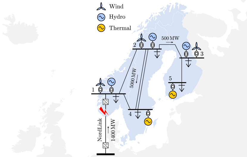
Figure 4: One-line diagram of the N5 test system. The system is implemented in Simulink and is available at https://github.com/joakimbjork/Nordic5.

The Nordic system currently applies two types of FCR: FCR for normal operation, within $\text{50.0}\pm\text{$0.1\text{\,}\mathrm{Hz}\text{/}$}$; and FCR for disturbance situations (FCR-D), activated when the frequency falls below $49.9\text{\,}\mathrm{Hz}\text{/}$. FCR-D have a faster response time and is designed to limit the maximum instantaneous frequency deviation to $49.0\text{\,}\mathrm{Hz}\text{/}$, and to stabilize the system at $49.5\text{\,}\mathrm{Hz}\text{/}$ [21].

The kinetic energy of the system varies greatly over the year, since the amount of synchronous generation connected to the grid depends on the demand [22]. For this analysis, we consider a low-inertia scenario with $W_{\mathrm{kin}}=$110\text{\,}\mathrm{GWs}\text{/}$$ distributed according to Table I. Assume that we have constant power loads with a combined frequency dependency of $400\text{\,}\mathrm{MW}\text{/}\mathrm{Hz}$ and consider the dimensioning fault to be the loss of a $1400\text{\,}\mathrm{MW}\text{/}$ importing dc link. The FCR-D requirements are then fulfilled in the average frequency model (15) if the total FCR amount to

$$F_{\mathrm{des}}(s)=k\frac{6.5s+1}{(2s+1)(17s+1)},$$ (31)

where $k=$3100\text{\,}\mathrm{MW}\text{/}\mathrm{Hz}$$ [18]. For the analysis, we let the bus dynamics be

$$g_{i}(s)=\frac{1}{s}\frac{1}{sM_{i}+F_{i}(s)+D_{i}},\quad i\in\{1,\ldots,5\},$$ (32)

where $M_{i}\geq 0$ is the inertia and $D_{i}\geq 0$ is the frequency dependent load at bus $i$, distributed according to Table I. In practice, $D_{i}$ is most likely unknown. Therefore, a conservative assumption is to assume that $D_{i}=0$ in the analysis. The frequency-dependent actuator

$$F_{i}(s)=H_{i}(s)K_{i}(s)$$ (33)

represent a feedback controller $K_{i}(s)$ and a controllable actuator $H_{i}(s)$. We consider two types of controllable actuators, hydro and wind.

The hydro governor implemented in this work is an adaptation of the model available in the Simulink Simscape Electrical library [23]. It has been modified to allow for a general linear FCR controller, $K(s)$, instead of the fixed PID/droop control structure, as shown in Fig. 5. The servo rate limit is set to the default $\pm$0.1\text{\,}\mathrm{p.u.}\text{/}\mathrm{s}$$. The nonlinear second-order model is useful for large-signal time-domain simulations. For the linear analysis, the turbine is modeled as

$$H_{\textrm{hydro}}(s)=2\frac{z-s}{s+2z}\frac{1}{sT_{y}+1},\quad z=\frac{1}{g_{0}T_{\mathrm{w}}}$$ (34)

where $T_{y}$ is the servo time constant, $g_{0}$ the initial gate opening, $T_{\mathrm{w}}$ the water time constant, $\hat{\omega}$ the locally measured frequency, and $\omega_{\mathrm{ref}}$ the frequency reference.

Figure 5: Block diagram of the hydro turbine and governor model.

Wind turbines participating in FFR are based on an adapted version of the National Renewable Energy Laboratory (NREL) $5\text{\,}\mathrm{MW}\text{/}$ baseline wind turbine model [24]. We consider uncurtailed operation below the rated wind speed. To allow for FFR while tracking the maximum power point (MPP), the control system has been modified according to [19] by adding a stabilizing feedback controller as illustrated in Fig. 6. For the linear analysis, the wind turbine is modeled as

$$H_{\mathrm{wind}}(s)=\frac{s-z}{s+k_{\mathrm{stab}}-z},\quad z=v\,C_{\Omega}$$ (35)

where $v$ is the wind speed, $k_{\mathrm{stab}}$ is the stabilizing feedback gain, and $C_{\Omega}$ is a variable that depends on how much the active power $P_{m}$ decreases when the rotor speed $\Omega$ deviates from the optimal rotor speed $\Omega_{\mathrm{MPP}}$. If we allow the turbine to operate down to $80\text{\,}\mathrm{\char 37\relax}\text{/}$ of $\Omega_{\mathrm{MPP}}$, then $C_{\Omega}\leq C_{0.8}=5.8\cdot 10^{-3}$. Setting the parameter $z=v\,C_{0.8}$ in (35) and $k_{\mathrm{stab}}=2v\,C_{0.8}$ then gives us a linear representation that overestimates the negative phase shift of $H_{\mathrm{wind}}(j\omega)$. In this way, we can use the linear model for a conservative stability analysis.

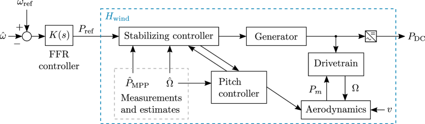
Figure 6: Block diagram of the wind turbine model.

Table I: Kinetic energy, load damping, and the network incidence parameters 19 for the $110\text{\,}\mathrm{GWs}\text{/}$ test case.

Bus	$W_{\mathrm{kin}}$ [$\mathrm{GWs}\text{/}$]	$D$ [$\mathrm{MW}\text{/}\mathrm{Hz}$]	$\gamma/2\pi$ [$\mathrm{GW}\text{/}\mathrm{rad}$]
1	34	150	6.2
2	22.5	60	10.2
3	7.5	20	5.2
4	33	120	7.5
5	13	50	3.0

VI-B Hydro–FCR

Let us derive a decentralized stability criterion for a system in which controllable frequency reserves are solemnly provided by the hydro turbines at buses 1, 2, and 3. Let the parameter and FCR resources be distributed according to Table II and let the FCR feedback controller be tuned using the model matching method presented in [18]. At bus $i$ we have

$$K_{i}(s)=c_{i}F_{\mathrm{des}}(s)\hat{H}_{\mathrm{hydro},i}^{-1}(s)$$ (36)

where the constant $c_{i}$ is the share of the total FCR so that $c_{1}+c_{2}+c_{3}=1$. The transfer function $F_{\mathrm{des}}(s)$ is the FCR design target 31, and $\hat{H}_{\mathrm{hydro},i}(s)$ is a minimum phase (MP) estimate of (34). With (36), the controllable frequency-dependent actuator

$$F_{\mathrm{hydro},i}(s)=K_{i}(s){H}_{\mathrm{hydro},i}(s)=c_{i}F_{\mathrm{des}}(s)\frac{z_{i}-s}{z_{i}+s}.$$ (37)

Since $H_{\mathrm{hydro}}(s)$ is NMP, the agent

$$g_{i}(s)=\frac{1}{s}\frac{1}{sM_{i}+F_{\mathrm{hydro},i}(s)+D_{i}}$$ (38)

may have unstable poles. With the FCR controller (36), the agents do in fact have unstable poles. As shown in Fig. 7a the unstable poles of agents (38) lies fairly close to the origin. Here, the unstable poles lie around $0.50\text{\,}\mathrm{rad}\text{/}\mathrm{s}$. The slowest interarea mode is known to be around $0.37\text{\,}\mathrm{Hz}\text{/}$ ($\approx$ $2.32\text{\,}\mathrm{rad}\text{/}\mathrm{s}$). It is therefore quite easy to find a suitable modified Nyquist $\mathcal{D}_{r}$-contour that excludes the unstable poles. In Fig. 7, we choose $r=$0.75\text{\,}\mathrm{rad}\text{/}\mathrm{s}$$. To derive a decentralized stability criterion using Corollary 1.2, we look at the field of values 30, spanned by vertices $\gamma_{i}g_{i}(s)$, as $s$ goes clockwise around the $\mathcal{D}_{r}$-contour.

Table II: Machine parameters for the $110\text{\,}\mathrm{GWs}\text{/}$ test case. Time constants and distribution of FCR are based on the case study in [25].

Bus	$P_{\mathrm{gen}}$ [$\mathrm{MW}\text{/}$]	FCR [$\mathrm{\char 37\relax}\text{/}$]	$T_{y}$	$T_{\mathrm{w}}$	$g_{0}$
1	$9000\text{\,}\hfil\lx@intercol&$ 60	0.2	0.7	0.8
2	$6000\text{\,}\hfil\lx@intercol&$ 30	0.2	1.4	0.8
3	$2000\text{\,}\hfil\lx@intercol&$ 10	0.2	1.4	0.8
4	$5000\text{\,}\hfil\lx@intercol&$ –	–	–	–
5	$2000\text{\,}\hfil\lx@intercol&$ –	–	–	–

Load Damping Excluded

Since we do not control the frequency dependent loads $D_{i}$, $i\in\{1,\ldots,5\}$, a reasonable conservative modeling assumption is to let $D_{i}=0$. In Fig. 7b we see that we cannot derive a stability criterion with the proposed controller (36) since the vertices that span the field of value approaches the origin from the top-left quadrant, thereby encircling $-1$. In fact, the analysis suggests that the system is unstable, without other sources that contribute to damping. To amend this, we may either modify the FCR controller 36 or assume that we know the frequency dependent loads $D_{i}>0$ and include these in the analysis. Here, we will use the latter, since this provides a good analogy to the case where we supplement hydro–FCR with wind–FFR in Section VI-C.

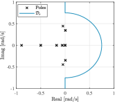
(a) Open-loop poles of $\mathcal{G}^{\prime}(s)$ and a modified Nyquist $\mathcal{D}_{r}$-contour that avoid any RHP poles slower than $r$.

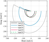
(b) The image of vertices $\gamma_{i}g_{i}(s)\in\mathcal{G}^{\prime}(s)$ as $s$ goes on the positive imaginary part of the $\mathcal{D}_{r}$-contour.

Figure 7: Open-loop poles and vertices of the N5 test system with hydro–FCR, assuming that the frequency dependent load $D_{i}=0$, $i\in\{1,\ldots,5\}$.

Load Damping Included

Assume that the distribution of the frequency dependent loads shown in Table I is known and that we therefore can include these in the analysis. With $D_{i}>0$, the trajectories move towards the bottom left quadrant, at least for higher frequencies where $D_{i}>|F_{\mathrm{hydro},i}(j\omega)|$. As the vertices move towards the bottom left quadrant, they no longer encircle $-1$. However, we see that vertices 1, 2, and 3 still go back up into the top-left quadrant to the left of $-1$. Therefore, the system has a lower gain margin $\alpha>0$. This is a problem since Corollaries 1.1 and 1.2 requires that the field of values $\alpha\operatorname{\mathrm{F}}\big{(}\mathcal{G}^{\prime}(s)\big{)}$, $\alpha\in(0,1]$, does not encircle $-1$. That is, none of the vertices are allowed to be left of $-1$ in the top left quadrant. Using Corollary 1.2 we can circumvent this problem by only looking on the image of vertices $\gamma_{i}g_{i}(s)$ for $s\in\mathcal{D}_{r}$. Setting the inner radius $r$ sufficiently large, we eventually find a point where the field of values cannot encircle $-1$. If frequency-dependent loads are distributed according to Table I, then we need $r$ to be larger than $0.37\cdot 2\pi$ $\mathrm{rad}\text{/}\mathrm{s}$, as seen in Fig. 8. Corollary 1.2 then tells us that we cannot have any unstable interarea modes with a eigenfrequency faster than $0.37\text{\,}\mathrm{Hz}\text{/}$, which we know to be the lower bound for the high-inertia operating condition.

Remark 2

For this low-inertia scenario, we know that the slowest interarea mode will have an eigenfrequency around $0.49\text{\,}\mathrm{Hz}\text{/}$. We can therefore safely say that no interarea mode will be destabilized by the hydro–FCR.

The simulated response to a $5\text{\,}\mathrm{s}\text{/}$ disconnection of the $1400\text{\,}\mathrm{MW}\text{/}$ importing dc link is shown in Fig. 9. The frequency deviation (top left) is limited by the help of hydro–FCR (bottom left) and the frequency-dependent loads (top center). The dc fault excites the north–south interarea mode, which is clearly visible on the tie-line flows (bottom-center). The stability of the system is aided by fast frequency-dependent loads, but network losses and voltage dynamics also play a role. For example, fast-acting excitation control, used to maintain the machine terminal voltage (top right), has a destabilizing effect on the interarea modes [10]. To mitigate the destabilizing effect of the voltage control, power system stabilizers (PSSs) (bottom-right) have been installed on the machines.

(a) Open-loop poles of $\mathcal{G}^{\prime}(s)$ and two modified Nyquist $\mathcal{D}_{r}$-contours with different radii.

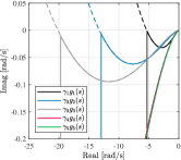
(b) The image of vertices $\gamma_{i}g_{i}(s)\in\mathcal{G}^{\prime}(s)$ as $s$ goes on the positive imaginary part of the two $\mathcal{D}_{r}$-contours.

Figure 8: Open-loop poles and vertices of the N5 test system with hydro–FCR, assuming that the distribution of the frequency dependent loads are known.

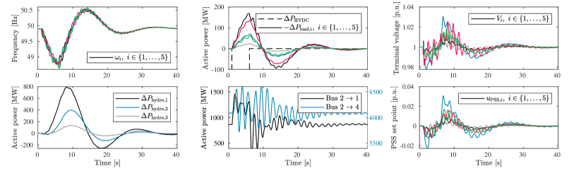
Figure 9: Simulation of a $5\text{\,}\mathrm{s}\text{/}$ disconnection of a $1400\text{\,}\mathrm{MW}\text{/}$ importing dc link in the N5 test system with hydro–FCR (37).

VI-C Hydro–FCR Supplemented with Wind–FFR

Let us now consider the case where we supplement hydro–FCR with wind–FFR at buses 1, 2, and 3. The obvious advantage of this approach is that the wind–FFR is a conscious design choice. We do not have to base our stability analysis on assumptions about the load behaviour as we did in Section VI-B. Note that we have chosen a positive real design target (31), so

$$\operatorname{\mathrm{Re}}\big{(}F_{\mathrm{des}}(j\omega)\big{)}\geq 0,\quad\forall\omega\geq 0.$$ (39)

Using the model matching design proposed in [18], we could design a supplementary wind–FFR so that the combined FCR and FFR at bus $i$ matches $c_{i}F_{\mathrm{des}}(s)$. As a result, all of the vertices would be negative imaginary

$$\operatorname{\mathrm{Im}}\big{(}\gamma_{i}g_{i}(j\omega)\big{)}\leq 0,\quad\forall\omega\geq 0$$ (40)

and therefore unable to encircle $-1$. In practice, however, it will likely not be possible to achieve strictly positive real frequency reserves. Even if we do not have dynamic limitations in the form of NMP zeros, such as with hydro power, we will always have time delays. Here, we will show how Corollaries 1.1 and 1.2 can be used to define a decentralized stability criterion even for a heterogeneous network with time delays.

To complement the hydro–FCR we let the wind turbines at buses 1, 2, and 3 participate in FFR. As mentioned earlier, this can be done using the model matching [18]. To make the result comparable to Section VI-B, however, we design the wind–FFR as a proportional frequency controller, making it comparable to the frequency-dependent load. Let

$$F_{\mathrm{wind},i}(s)=c_{i}k_{\mathrm{FFR}}\frac{5se^{-s\tau_{i}}}{5s+1}{H}_{\mathrm{wind},i}(s),$$ (41)

for $i\in\{1,2,3\}$, where we choose $k_{\mathrm{FFR}}=$1000\text{\,}\mathrm{MW}\text{/}\mathrm{Hz}$$. Since power outtake makes the wind turbine deviate from the MPP, it cannot provide any sustained control action. This behaviour is captured by the all-pass characteristic in (35). The turbines are able to achieve tight control at frequencies above $0.06\text{\,}\mathrm{rad}\text{/}\mathrm{s}$, i.e., they are well capable of damping interarea modes. Using a washout filter with a lower bandwidth of $0.2\text{\,}\mathrm{rad}\text{/}\mathrm{s}$ we avoid steady control action. It is fairly straightforward to show that the wind farm and the hydro unit form a locally stable subsystem at bus 1, 2, and 3, respectively. For analyzing the global stability, the agents to consider then becomes

$$g_{i}(s)=\frac{1}{s}\frac{1}{sM_{i}+F_{\mathrm{hydro},i}(s)+F_{\mathrm{wind},i}(s)}$$ (42)

for $i\in\{1,2,3\}$, and

$$g_{i}(s)=\frac{1}{s}\frac{1}{sM_{i}}$$ (43)

for $i\in\{4,5\}$. For simplicity, assume that the network incidence parameters $\gamma_{i}$, for the hydro–wind subsystems, are the same as in Section VI-C. Let the wind speed and power rating be distributed according to Table III. Furthermore, lets assume that the delay $\tau_{i}=\tau=$100\text{\,}\mathrm{ms}\text{/}$$ at all buses. Under these circumstances, neither of the vertices encircles the point $-1$, as seen in Fig. 11. The proposed wind–FFR is stronger than the frequency dependent load shown in Fig. 8b. As a result, there is no risk for slow instability due to vertices entering the top left quadrant to the left of $-1$. Unlike the example with frequency-dependent loads, however, the vertices that correspond to agents with wind–FFR cross over the real axis to the right of $-1$. The reason for this is the time delay in (41). Consequently, we risk fast instability. If we neglect the hydro–FFR, then $\gamma_{i}g_{i}(s)$, $i\in\{1,2,3\}$ cross over the real axis exactly at $s=j\pi/2\tau$. This implies that a network with stronger connectivity (larger $\gamma_{i}$) will be more sensitive to fast instability caused by time delays.

Table III: Wind turbine parameters for the $110\text{\,}\mathrm{GWs}\text{/}$ test case.

Bus	$P_{\mathrm{nom}}$ [$\mathrm{MW}\text{/}$]	FFR [$\mathrm{\char 37\relax}\text{/}$]	$v$ [$\mathrm{m}\text{/}\mathrm{s}$]	$P_{\mathrm{MPP}}$ [$\mathrm{MW}\text{/}$]
1	$1000\text{\,}\hfil\lx@intercol&$ 60	10	695
2	$1000\text{\,}\hfil\lx@intercol&$ 30	6	150
3	$500\text{\,}\hfil\lx@intercol&$ 10	7	120

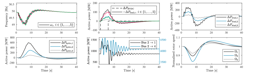
Figure 10: Simulation of a $5\text{\,}\mathrm{s}\text{/}$ disconnection of a $1400\text{\,}\mathrm{MW}\text{/}$ importing dc link in the N5 test system with hydro–FCR (37) and wind–FFR (41).

The simulated response to a $5\text{\,}\mathrm{s}\text{/}$ disconnection of the $1400\text{\,}\mathrm{MW}\text{/}$ importing dc link is shown in Fig. 10. Apart for the assisting wind–FFR, the setup is identical to the system setup used in Fig. 9. As can be seen in the frequency response (top-left) and the north–south tie-line flows (bottom-center), the wind–FFR (top-right) not only improves the frequency disturbance attenuation, but also improves the attenuation of interarea modes. The power excursion during FFR decelerates the wind turbines (bottom-right). However, they are still within the allowed operating range, above $80\text{\,}\mathrm{\char 37\relax}\text{/}$ of the normalized rotor speed $\Omega/\Omega_{\mathrm{MPP}}$.

VI-D Summary: A Scalable Nyquist Stability Criterion.

The following algorithm can be used as a blue print for a decentralized scalable Nyquist stability criterion.

• Define a modified Nyquist $\mathcal{D}_{r}$-contour, a separating hyperplane, and a time constant $\tau_{\mathrm{max}}$, to be used by all agents in the network.

• We need an estimate of the lower bound for the local inertia $M_{i}\geq 0$ and an estimate of the controller and actuator dynamics $F_{i}(s)$ of devices that we want to connect. We also need to know an upper bound on the local network incidence parameter $\gamma_{i}$. We then require that

  1. the agent $g_{i}(s)$ does not have unstable poles inside the modified Nyquist $\mathcal{D}_{r}$-contour,

  2. the vertex $\gamma_{i}g_{i}(s)$ does not enter the top-left quadrant to the left of $-1$ as $s$ goes along the positive imaginary part of the $\mathcal{D}_{r}$-contour, and that

  3. the vertex $\gamma_{i}g_{i}(j\omega)$ lies to the right of the hyperplane for all $\omega>\pi/2\tau_{\mathrm{max}}$.

If every agent that connects to the network fulfills these criteria, then the network has no unstable interarea mode with an eigenfrequency faster than $r$. The frequency of slow system-wide interarea modes are easily observable from phasor measurements. The required bound for $r$ should therefore be well known by the system operator. Note that in Fig. 11b, agents $i\in\{4,5\}$ do not participate in frequency control. It is therefore impossible to base the stability criterion solemnly on a separating hyperplane in the Nyquist diagram.

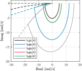
(a) The image of vertices 42 and 43 as $s$ goes on the positive imaginary part of the $\mathcal{D}_{r}$-contours in Fig. 8a.

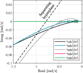
(b) Zoom in around $-1$. The “$\times$” marks the value of vertex $\gamma_{i}g_{i}(j\omega)$ at $\omega=\pi/2\tau$.

Figure 11: Vertices of the N5 test system with hydro–FCR and wind–FFR.

VII Conclusions

A scalable, decentralized stability criterion has been derived for a network with heterogeneous agents. Stability is assessed without making prior assumptions on network losses or dynamics by directly applying the generalized Nyquist criterion on the field of values spanned by the agents. Using the proposed method, local stability criteria were derived for systems where passivity or separating hyperplane methods are impossible, e.g. if we have a mix of time-delayed actuators and uncontrolled agents. The results were validated in a detailed nonlinear power system model where we studied hydro–FCR and wind–FFR. It was shown that if actuators have slow RHP zero dynamics (as is typically the case for hydro governors), then the local bus dynamics (the agent) may be unstable. As long as the frequency of the slowest interarea mode is known, it is possible to define a decentralized stability criterion, even for a network with unstable agents.

Typically, power system stability are separated into frequency, rotor angle, and voltage stability. These are typically treated separately. This work presents a unified framework for analyzing both frequency and rotor angle stability. The results show that we risk destabilizing the interarea modes if we demand bandwidth limited actuators, such as NMP hydro turbines, to provide fast reserve power in low inertia power systems. It was shown that a convenient way to mitigate this problem is to allow converter-interfaced generation, capable of fast control action, to assist the conventional slow reserves. For our future work, we will extend the result to second-order network dynamics so that we can include voltage dynamics in the stability analysis.

References

- [1] R. Pates and E. Mallada, “Robust scale-free synthesis for frequency control in power systems,” IEEE Control Netw. Syst., vol. 6, no. 3, pp. 1174–1184, Sep. 2019.
- [2] S. Baros, A. Bernstein, and N. D. Hatziargyriou, “Distributed conditions for small-signal stability of power grids and local control design,” IEEE Trans. Power Syst., vol. 36, no. 3, pp. 2058–2067, May 2021.
- [3] N. Monshizadeh and I. Lestas, “Secant and Popov-like conditions in power network stability,” Automatica, vol. 101, pp. 258–268, Mar. 2019.
- [4] P. Yang, F. Liu, Z. Wang, and C. Shen, “Distributed stability conditions for power systems with heterogeneous nonlinear bus dynamics,” IEEE Trans. Power Syst., vol. 35, no. 3, pp. 2313–2324, May 2020.
- [5] F. Paganini and E. Mallada, “Global analysis of synchronization performance for power systems: Bridging the theory-practice gap,” IEEE Trans. Autom. Control, vol. 65, no. 7, pp. 3007–3022, Jul. 2020.
- [6] J. A. Fax and R. M. Murray, “Information flow and cooperative control of vehicle formations,” IEEE Trans. Autom. Control, vol. 49, no. 9, pp. 1465–1476, Sep. 2004.
- [7] A. Gattami and R. Murray, “A frequency domain condition for stability of interconnected MIMO systems,” in Proceedings of the 2004 American Control Conference, vol. 4, Boston, MA, Jun. 2004, pp. 3723–3728.
- [8] R. Olfati-Saber, J. A. Fax, and R. M. Murray, “Consensus and cooperation in networked multi-agent systems,” Proceedings of the IEEE, vol. 95, no. 1, pp. 215–233, Jan. 2007.
- [9] F. Bullo, Lectures on Network Systems. Kindle Direct Publishing, 2020.
- [10] P. Kundur, Power System Stability and Control. New York: McGraw-Hill, 1994.
- [11] J. M. Maciejowski, Multivariable Feedback Design, ser. Electronic Systems Engineering Series. Wokingham, England: Addison-Wesley, 1989.
- [12] I. Postlethwaite and A. G. J. MacFarlane, A Complex Variable Approach to the Analysis of Linear Multivariable Feedback Systems. Berlin, Germany: Springer, 1979, no. 12.
- [13] S. Skogestad and I. Postlethwaite, Multivariable Feedback Control: Analysis and Design, 2nd ed. New York: Wiley, 2007.
- [14] K. Zhou, Robust and Optimal Control. Englewood Cliffs, NJ: Prentice Hall, 1996.
- [15] J. W. Brown and R. V. Churchill, Complex Variables and Applications, 7th ed. Boston, MA: McGraw-Hill Higher Education, 2004.
- [16] R. A. Horn and C. R. Johnson, Topics in Matrix Analysis, 1st ed. Cambridge, UK: Cambridge University Press, 1991.
- [17] F. Dörfler and F. Bullo, “Kron reduction of graphs with applications to electrical networks,” IEEE Trans. Circuits Syst. I, Reg. Papers, vol. 60, no. 1, pp. 150–163, Jan. 2013.
- [18] J. Björk, K. H. Johansson, and F. Dörfler, “Dynamic virtual power plant design for fast frequency reserves: Coordinating hydro and wind,” IEEE Control Netw. Syst., to be published.
- [19] J. Björk, D. V. Pombo, and K. H. Johansson, “Variable-speed wind turbine control designed for coordinated fast frequency reserves,” IEEE Trans. Power Syst., pp. 1–11, 2021.
- [20] J. Björk, “Fundamental control performance limitations for interarea oscillation damping and frequency stability,” Ph.D. dissertation, KTH Royal Institute of Technology, Stockholm, Sweden, 2021.
- [21] ENTSO-E, “Nordic synchronous area proposal for the frequency quality defining parameters and the frequency quality target parameter in accordance with Article 127 of the Commission Regulation (EU) 2017/1485 of 2 August 2017 establishing a guideline on electricity transmission system operation,” 2017.
- [22] ——, “Fast frequency reserve – solution to the Nordic inertia challenge,” Tech. Rep., 2019.
- [23] Hydro-Québec and The MathWorks, “Simscape Electrical Reference (Specialized Power Systems),” Natick, MA, Tech. Rep., 2020.
- [24] J. Jonkman, S. Butterfield, W. Musial, and G. Scott, “Definition of a 5-MW reference wind turbine for offshore system development,” NREL, USA, Tech. Rep., 2009.
- [25] L. Saarinen, P. Norrlund, U. Lundin, E. Agneholm, and A. Westberg, “Full-scale test and modelling of the frequency control dynamics of the Nordic power system,” in IEEE Power and Energy Society General Meeting, Boston, MA, Jul. 2016.