Privacy-preserving Data Sharing on Vertically Partitioned Data

Abstract

In this work, we introduce a differentially private method for generating synthetic data from vertically partitioned data, i.e., where data of the same individuals is distributed across multiple data holders or parties. We present a differentially privacy stochastic gradient descent (DP-SGD) algorithm to train a mixture model over such partitioned data using variational inference. We modify a secure multiparty computation (MPC) framework to combine MPC with differential privacy (DP), in order to use differentially private MPC effectively to learn a probabilistic generative model under DP on such vertically partitioned data. Assuming the mixture components contain no dependencies across different parties, the objective function can be factorized into a sum of products of the contributions calculated by the parties. Finally, MPC is used to compute the aggregate between the different contributions. Moreover, we rigorously define the privacy guarantees with respect to the different players in the system. To demonstrate the accuracy of our method, we run our algorithm on the Adult dataset from the UCI machine learning repository, where we obtain comparable results to the non-partitioned case.

1 Introduction

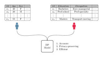
Figure 1: Basic Idea of the problem: Multiple parties hold different sets of features for the same set of individuals. We want to train a DP model of the combined set that is accurate, efficient, and privacy-preserving, without the partners sharing their data with each other.

Differential privacy (DP) (Dwork et al.,, 2006) provides a framework for developing algorithms that can use sensitive personal data while guaranteeing the privacy of the data subjects. One of the most interesting applications of DP is data anonymisation Samarati and Sweeney, (1998); Sweeney, (2002) through creating an anonymised twin of a dataset. The anonymised dataset can then be used in place of the original for new analyses, while maintaining privacy for the original data subjects. In this paper, we investigate the problem of learning mixture models for vertically partitioned data under DP, as shown in Figure 1, where multiple parties hold different features for the same set of individuals. Privacy-preserving learning for vertically partitioned data would enable addressing completely new questions through combining for example health and shopping data that are held by different parties who cannot otherwise combine their data.

Creating synthetic data to ensure anonymity was first proposed by Rubin, (1993). After the introduction of DP, several authors have proposed methods for releasing synthetic data protected by DP guarantees (e.g. Blum et al.,, 2008; Dwork et al.,, 2009; Xiao et al.,, 2010; Beimel et al.,, 2010; Chen et al.,, 2012; Hardt et al.,, 2012; Zhang et al.,, 2014). Recent work has focused on applying generative machine learning models learned under DP using autoencoder neural networks (e.g. Acs et al.,, 2018), generative adversarial networks (GANs) (e.g. Yoon et al.,, 2019), discrete data generation using probabilistic graphical models Zhang et al., (2014); McKenna et al., (2019) or more general probabilistic models (Jälkö et al.,, 2021). DP provides a formal guarantee that the true data cannot be inferred from the generated synthetic data, something that would be very difficult to guarantee with other methods.

The data are often distributed across multiple parties. The most typical distributed data case is so-called horizontal partitioning, where different parties hold data for different individuals. This setting is the basis for federated learning (Kairouz et al.,, 2019) which can be used to learn models by combining updates from multiple parties holding data for different individuals. Another setting is the vertical data partitioning, in which the data are divided such that each party holds different features of the same set of individuals.

While the literature is broad on DP learning on horizontally partitioned data, there has only been very limited prior work on DP learning on vertically partitioned data. Mohammed et al., (2013) proposed an algorithm for secure two-party DP data release for vertically partitioned data, but their algorithm is limited to discrete data with a small number of possible values because it requires enumerating all possible values of a data element. Recently Wang et al., (2020) proposed a method for DP learning of generalised linear models on vertically partitioned data.

Secure multiparty computation (MPC) (Yao,, 1982; Maurer,, 2006) is a cryptographic technique to allow multiple parties to compute a function of their private inputs without revealing their inputs. Running the learning algorithm under MPC would in theory solve the privacy concern arising from vertical partitioning, but directly using MPC for large problems would be a bottleneck since it is computationally expensive. In this work, we limit the use of MPC to the final gradient aggregation which comprises of a few simple operations, in order to reduce the computational cost. We do this using a slightly modified version of CrypTen (Gunning et al.,, 2019), which adds MPC to PyTorch.

In addition to the challenge of securely combining the contributions of different parties, vertical data partitioning introduces the additional challenge of matching the records between different parties. For simplicity, we assume the records have been matched before running our algorithm. If necessary, the data can be matched first using a private entity resolution algorithm (Getoor and Machanavajjhala,, 2012; Sehili et al.,, 2015).

In this work, we propose an algorithm for DP data sharing by applying differentially private variational inference (DPVI) and MPC to train a mixture model on vertically partitioned data, where we can privately infer the parameters of the distribution of the data. The algorithm requires gradients of parameters based on the data, which we form such that each party computes only dimensions matching to its data. This information is combined using MPC, where the parties combine the gradients and use the typical DP-SGD operations of clipping and perturbing the gradients in every optimisation iteration. To the best of our knowledge, this is the first work to build a DP-SGD algorithm for vertically partitioned data. Particularly, we make the following contributions:

• We provide an algorithm for training a mixture model on vertically partitioned data based on DP variational inference. This algorithm is generalizable to any model where the log likelihood does not have any direct dependencies among the parties.

• We rigorously define the privacy guarantees with respect to the different players in the system, i.e., the outside analyst and the parties.

• We show that the performance of the algorithm is comparable to the non-partitioned DPVI algorithm by running both algorithms on the Adult dataset.

• The algorithm studied in this work requires high precision, which is not directly possible using the MPC framework Crypten. To solve this, we provide a method to modify the Crypten arithmetics for MPC to allow more precision in the fixed point representation. These additions could be easily used whenever a need for more precision arises.

The outline of the paper is as follows: In Section 2, we describe the preliminaries needed for this work. Afterwards in Section 3, we will descibe the problem setup and theoretical analysis of the privacy protocol. In Section 4, we describe the algorithm for training on vertically partitioned data. After defining the model, we state our privacy guarantees in Section 5. In Section 6, we provide results from experiments on the Adult dataset Dua and Graff, (2017) showing that the accuracy of the model is on-par with the non-partitioned case. Then we conclude with discussions and conclusions in Sections 7 and 8.

2 Preliminaries

2.1 Differential Privacy (DP)

Differential privacy (DP) (Dwork et al.,, 2006; Dwork and Roth,, 2014) is a framework allowing learning significant information about a population, while learning almost nothing about any certain individual. DP provides a strong mathematical guarantee of privacy.

Definition 2.1 (($\epsilon,\delta$)-Differential Privacy).

Let $\epsilon,\delta\geq 0$. A randomised algorithm $\mathcal{A}$ is ($\epsilon,\delta$)-differentially private if for all pairs of adjacent datasets $\mathcal{D},\mathcal{D}^{\prime}$, i.e., differing in one data sample, and all measurable subsets $S\subset\operatorname{im}(\mathcal{A})$

$$\Pr(\mathcal{A}(\mathcal{D})\in S)\leq e^{\epsilon}\Pr(\mathcal{A}(\mathcal{D}^{\prime})\in S)+\delta.$$

The case $\delta=0$, is known as $\epsilon$-differentially privacy, or pure DP. The parameters $\epsilon,\delta$ measure the strength of the privacy, where smaller values correspond to stronger privacy.

2.1.1 DP stochastic gradient descent

One of the most general and widely applied DP learning techniques is the DP stochastic gradient descent (DP-SGD) (Rajkumar and Agarwal,, 2012; Song et al.,, 2013; Abadi et al.,, 2016), where the parameters of a differentiable loss function $\mathcal{L}(\boldsymbol{\theta},\mathcal{D})=\sum_{i}\mathcal{L}_{i}(\boldsymbol{\theta},\boldsymbol{x}_{i})$ are learned under DP. Here $\boldsymbol{\theta}$ are the parameters of the model and $\mathcal{D}=\{\boldsymbol{x}_{i}\}_{i=1}^{N}$ is the dataset. For loss functions which can be represented as a sum over elements of a dataset, DP-SGD computes the gradients w.r.t. the parameters for each individual, $\boldsymbol{g}_{i}=\nabla_{\boldsymbol{\theta}}\mathcal{L}_{i}(\boldsymbol{\theta},\boldsymbol{x}_{i})$, on a randomly sampled subset of the data. The individual gradients $\boldsymbol{g}_{i}$ are then projected into $B^{d}(0,C)$, a $d$-dimensional ball with radius $C$, where $d$ is the number of parameters, and finally summed and perturbed with spherical Gaussian noise with covariance matrix $C^{2}\sigma^{2}\boldsymbol{I}_{d}$, where $\boldsymbol{I}_{d}$ is the $d$-dimensional identity matrix and noise variance $\sigma^{2}$ controls the magnitude of added noise.

2.1.2 Privacy accounting

In order to formalise computing the privacy properties of a complex composition of DP mechanisms such as used in DP-SGD, we define the concept of an accounting oracle that can be used to obtain the privacy bounds.

Definition 2.2 (Accounting Oracle).

An $\epsilon$-accounting oracle or simply accounting oracle, is a function $\mathcal{O}$ that evaluates $(\epsilon,\delta)$-DP privacy bounds for compositions of subsampled mechanisms. Specifically, given $\delta$, sub-sampling ratio $q$, number of iterations $T$ and a base mechanism $\mathcal{A}(\sigma)$, the oracle gives an $\epsilon$, such that a $T$-fold composition of $\mathcal{A}(\sigma)$ with sub-sampling with ratio $q$ is $(\epsilon,\delta)$-DP, i.e.,

$$\mathcal{O}:(\delta,q,T,\mathcal{A})\mapsto\epsilon$$

There are a number of approaches for realising an accounting oracle, leading to increasingly tight bounds. The advanced composition theorem (Dwork and Roth,, 2014) gives simple analytical bounds given $(\epsilon,\delta)$-DP bounds for $\mathcal{A}(\sigma)$. Rényi DP (Mironov,, 2017) is a common approach for obtaining tighter bounds, but only numerical methods (Koskela et al.,, 2020) based on privacy loss distributions (Sommer et al.,, 2019) can realise an arbitrarily accurate oracle.

2.2 Variational Inference

In Bayesian statistics our goal is to learn the posterior distribution of parameters of a probabilistic model. For a probabilistic model $p(\mathcal{D},\boldsymbol{\theta})$, where $\mathcal{D}$ denotes the data and $\boldsymbol{\theta}$ the model parameters, the posterior distribution is given as

$$p(\boldsymbol{\theta}\mid\mathcal{D})=\frac{p(\mathcal{D}\mid\boldsymbol{\theta})p(\boldsymbol{\theta})}{p(\mathcal{D})}.$$ (1)

The exact posterior distribution is often intractable and we need to resort to approximate Bayesian inference. Variational inference (VI) approximates the intractable posterior distribution with a tractable variational posterior $q_{\boldsymbol{\xi}}(\boldsymbol{\theta})$ (Jordan et al.,, 1999).

We learn the variational posterior by minimizing the Kullback-Leibler divergence between the variational posterior $q_{\boldsymbol{\xi}}(\boldsymbol{\theta})$ and the true posterior $p(\boldsymbol{\theta}\mid\mathcal{D})$:

$$KL(q_{\boldsymbol{\xi}}(\boldsymbol{\theta})||p(\boldsymbol{\theta}\mid\mathcal{D}))=\mathbb{E}_{q_{\boldsymbol{\xi}}(\boldsymbol{\theta})}\left[\log\frac{q_{\boldsymbol{\xi}}(\boldsymbol{\theta})}{p(\boldsymbol{\theta}\mid\mathcal{D}))}\right]$$ (2)

Now, this expressions again involves the exact posterior which is intractable. Therefore, instead of directly optimizing the KL divergence, VI fits the approximate posterior $q_{\boldsymbol{\xi}}(\boldsymbol{\theta})$ by maximizing the evidence lower bound (ELBO) w.r.t. the variational parameters $\boldsymbol{\xi}$. The ELBO is given as

$$\mathcal{L} =\int q_{\boldsymbol{\xi}}(\boldsymbol{\theta})\log{\frac{p(\mathcal{D},\boldsymbol{\theta})}{q_{\boldsymbol{\xi}}(\boldsymbol{\theta})}}\,\mathrm{d}\boldsymbol{\theta}$$

$$=-KL(q_{\boldsymbol{\xi}}(\boldsymbol{\theta})||p(\boldsymbol{\theta}))+\sum_{i=1}^{N}\mathbb{E}_{q_{\boldsymbol{\xi}}(\boldsymbol{\theta})}\left[\log(p(\boldsymbol{x}_{i}|\boldsymbol{\theta}))\right]$$

$$=-KL(q_{\boldsymbol{\xi}}(\boldsymbol{\theta})||p(\boldsymbol{\theta}\mid\mathcal{D}))+\log p(\mathcal{D}),$$

where $\mathcal{D}=\{\boldsymbol{x}_{1},\cdots,\boldsymbol{x}_{N}\}$ is the set of observations, $\mathbb{E}_{q}$ denotes the expectation over distribution $q$ and $KL(q||p)$ the Kullback-Leibler divergence between $q$ and $p$ defined in Eq. (2).

The ELBO lower bounds the marginal likelihood $\log p(\mathcal{D})$, i.e., it is the evidence of the marginal likelihood, and thus the name. It is straightforward to see that setting $q_{\boldsymbol{\xi}}$ to the true posterior maximizes ELBO and therefore minimizes the Kullback-divergence.

2.2.1 Doubly stochastic variational inference

In certain models, a suitable choice of variational posterior leads to analytically tractable variational parameters. This however is not the case in general. Doubly stochastic variational inference (DSVI) Titsias and Lázaro-Gredilla, (2014) is a framework based on stochastic gradient optimisation of the ELBO. It operates on variational approximations that lead into a differentiable form of ELBO. For such approximation, the variational parameters $\boldsymbol{\xi}$ can be learned using a stochastic gradient optimiser. For instance, samples $\boldsymbol{\theta}$ from a Gaussian variational distribution $q_{(\boldsymbol{\mu},\boldsymbol{L})}(\boldsymbol{\theta})=\mathcal{N}(\boldsymbol{\theta};\boldsymbol{\mu},\boldsymbol{L}\boldsymbol{L}^{T})$ can be reparametised as $\boldsymbol{\theta}:=\boldsymbol{\theta}(\boldsymbol{\mu},\boldsymbol{L};\boldsymbol{\eta})=\boldsymbol{\mu}+\boldsymbol{L}\boldsymbol{\eta}$, where $\boldsymbol{\eta}\sim\mathcal{N(\mathbf{0},\mathbf{I})}$.

Denoting the parameters of the reparametrisation $\boldsymbol{\xi}:=(\boldsymbol{\mu},\boldsymbol{L})$, the sample $\boldsymbol{\theta}$ can be expressed as a stochastic function $\boldsymbol{\theta}(\boldsymbol{\xi};\boldsymbol{\eta})$ which is now differentiable w.r.t. the parameters $\boldsymbol{\mu},\boldsymbol{L}$, and thus the expression inside the expectation in ELBO is also differentiable w.r.t. the variational parameters. This means that we can optimise the variational parameters with gradients such as

$$\nabla_{\boldsymbol{\xi}}\mathcal{L} =\nabla_{\xi}\mathbb{E}_{\phi(\boldsymbol{\eta})}\left[\log\frac{p(\mathcal{D},\boldsymbol{\theta})}{q_{\boldsymbol{\xi}}(\boldsymbol{\theta})}\right]$$ (3)

$$=\mathbb{E}_{\phi(\boldsymbol{\eta})}\left[\nabla_{\boldsymbol{\xi}}\log\frac{p(\mathcal{D},\boldsymbol{\theta}(\boldsymbol{\xi};\boldsymbol{\eta}))}{q_{\boldsymbol{\xi}}(\boldsymbol{\theta}(\boldsymbol{\xi};\boldsymbol{\eta}))}\right]$$ (4)

$$=\mathbb{E}_{\phi(\boldsymbol{\eta})}\left[\nabla_{\boldsymbol{\xi}}\log\frac{p(\mathcal{D},\boldsymbol{\theta}(\boldsymbol{\xi};\boldsymbol{\eta}))|\det(J(\boldsymbol{\theta}))|}{\phi(\boldsymbol{\eta})}\right]$$ (5)

$$=\mathbb{E}_{\phi(\boldsymbol{\eta})}\left[\nabla_{\boldsymbol{\xi}}\left(\log p(\mathcal{D},\boldsymbol{\theta}(\boldsymbol{\xi};\boldsymbol{\eta}))+\log|\det(J(\boldsymbol{\theta}))|\right)\right]$$ (6)

$$=\mathbb{E}_{\phi(\boldsymbol{\eta})}\left[\nabla_{\boldsymbol{\xi}}\left(\log p(\mathcal{D},\boldsymbol{\theta}(\boldsymbol{\xi};\boldsymbol{\eta}))+\log|\det(\boldsymbol{L})|\right)\right],$$ (7)

where $\det(J(\boldsymbol{\theta}))=\det(\boldsymbol{L})$ denotes the determinant of the Jacobian of $\theta(\boldsymbol{\xi};\boldsymbol{\eta})$ w.r.t. the $\boldsymbol{\eta}$, and $\phi(\boldsymbol{\eta})$ is the density of $\boldsymbol{\eta}$.

The expectations with respect to $\phi(\boldsymbol{\eta})$ are evaluated using Monte Carlo integration. In many cases, a single Monte Carlo sample is sufficiently accurate for SGD. Therefore, we can drop the expectation.

To extend the approach for model parameters that are constrained, an Automatic Differentiation Variational Inference (ADVI) framework was proposed by Kucukelbir et al., (2017). In this framework the constrained variables are transformed into $\mathbb{R}^{d}$ with a bijective map. Next the unconstrained results are given a Gaussian variational distribution, and finally the ELBO is written using the change of variables rule for the constrained variables.

2.2.2 DP variational inference

Differentially private variational inference (DPVI) is a technique, first proposed in Jälkö et al., (2017), that learns the variational posteriors under differential privacy. The method is based on using DP-SGD for optimisation of the variational parameters.

2.3 Cryptographic Techniques

Cryptography is used in order for two or more parties to compute a function on their collective data without sharing their data with one another.

This paper will also discuss using cryptographic techniques to achieve DP. Discrete Gaussian noise will be added for the DP modelling, with privacy guarantees given in Kairouz et al., (2021), which is added under MPC.

Secure Multi-party Computation

Secure multi-party computation (MPC) (Yao,, 1982; Maurer,, 2006) is a cryptographic technique that allows parties to compute a function of their combined data without revealing the data to one another. One of the basic tools of MPC is the Shamir secret sharing scheme (Shamir,, 1979). A $t$-out-of-$n$ secret sharing scheme assumes a dealer who wants to share a secret with $n$ parties, where any $t$ players can reconstruct the secret, however, but any subset of $t-1$ or less parties cannot reconstruct it.

There are two general MPC protocols, Boolean MPC and arithmetic MPC. Boolean MPC is used to evaluate a Boolean circuit. This is based on Yao’s garbled circuits (Yao,, 1982). On the other hand, arithmetic MPC is used to evaluate arithmetic functions and is based on additive homomorphic encryption. Arithmetic MPC supports basic mathematical operations, such as addition and multiplication. Also, using MPC, one can approximate other arithmetic functions. However, the limitation of arithmetic MPC is that it cannot deal with floating point numbers, and therefore, a fixed point representation of real values must be used. There has been some work on MPC with floating point arithmetic such as the recent work by Guo et al., (2022), where approximations of functions, such as division and square roots, are derived on real numbers.

There are some general purpose software packages for MPC. In this paper, we will implement the method on CrypTen (Gunning et al.,, 2019) framework. CrypTen implements arithmetic and Boolean MPC for PyTorch. In our work, we will use the arithmetic MPC implementation.

2.4 Distributed Gaussian Noise addition

Canonne et al., (2020) showed that adding discrete Gaussian noise $\mathcal{N}_{\mathbb{Z}}(0,\sigma^{2})$ provides almost identical DP guarantees as the continuous Gaussian. A discrete distributed Gaussian mechanism for noise addition was introduced by Kairouz et al., (2021). It is shown that adding discrete Gaussian noise from each party can be summed up to get DP guarantees which match the non-distributed Gaussian noise addition DP. In Theorem 11 by Kairouz et al., (2021), it is stated that although the convolution of two discrete Gaussians is not a discrete Gaussian, it is very close to a discrete Gaussian. This theorem is also extended to the sum of more than two Gaussians.

3 Privacy model

3.1 Problem Setup

For vertically partitioned data, we assume the following players in the model:

• $P$ parties, i.e., data holders, where each party is holding a set of features for the same set of individuals.

• Central aggregator who is responsible for running the learning algorithm.

• An outside analyst who observes the data once it is published.

• Possible trusted third party, e.g. a trusted execution environment (TEE), which will add the noise.

The parties want to collaborate in order to learn a mixture model over their collective data. However, the information they own is private and cannot be shared among the parties. We will consider two options: the first is to assume each party adds a portion of the noise to the model, while the second is to assume that we have a trusted third party who will add the noise to the model before publishing the data.

The parties will communicate with one another under MPC, such that they only share encrypted information. Lastly, the model is symmetric, i.e., the privacy constraints on all parties are the same.

For notational convenience, we assume that the individuals are in the same order in all the parties’ datasets. We further assume that the parties are honest-but-curious, i.e., they would always answer honestly but would try to know more about the data from the other parties.

3.1.1 Noise addition

If we assume having a trusted third party (TEE), then this party will add a $\mathcal{N}_{\mathbb{Z}}(0,\sigma^{2})$ discrete Gaussian noise needed in the DP mechanism.

Otherwise, if we are assuming that there is no trusted third party in the model, the parties need to collaborate to add the DP noise. For that, each party will send its share of the discrete Gaussian noise in an encrypted form. The noise from the parties will have zero mean and $1/P$ the required noise variance, i.e. the noise of each party is sampled from $\mathcal{N}_{\mathbb{Z}}(0,\sigma^{2}/P)$, where $P$ is the number of parties. This noise is then summed together under MPC resulting in a sample from $\mathcal{N}_{\mathbb{Z}/P}(0,\sigma^{2})\approx\mathcal{N}_{\mathbb{Z}}(0,\sigma^{2})$ and added to the gradients before the decryption. The notation $\mathcal{N}_{\mathbb{Z}/P}$ is used here for a distributed discrete Gaussian formed of $P$ parts to highlight the fact that this is not identical to the plain discrete Gaussian.

3.2 Vertically Partitioned Differential Privacy

In the vertically partitioned data setting, each party holds a subset of the features. Therefore, with respect to each party, the data the other parties hold are secret, while the data it holds is known. However, the parties share the same individuals, and therefore contrary to the standard DP setting, the involvement of a single individual cannot be considered a secret between the parties. Thus, the privacy model of DP cannot we used when analyzing the privacy guarantees between the parties. Therefore, we need to introduce a new privacy notion. We start by defining the adjancency in the vertically partitioned setting.

Definition 3.1 (Vertically Partitioned Adjacency, VP-adjacency).

Let $\mathcal{D}$ and $\mathcal{D}^{\prime}$ be datasets with $M$ features. We assume that the features are partitioned over $P$ parties $1,\cdots,P$, where party $i$ holds $m_{i}$ features and $\sum_{i}m_{i}=M$. Moreover, let $x_{j}^{i}\in\mathcal{D}$ be the portion of sample $x_{j}$ held by party $i$ and ${x_{j}^{i}}^{\prime}\in\mathcal{D}^{\prime}$ be the portion of sample $x_{j}^{\prime}$ held by party $i$. We say $\mathcal{D}$ and $\mathcal{D}^{\prime}$ are VP-adjacent if $\mathcal{D}=\mathcal{D}^{\prime}\setminus\{x_{k}\}\cup\{x_{k}^{\prime}\}$ for some $k\in[N]$, such that $x_{k}^{p}={x_{k}^{p}}^{\prime}$ for some party $p\in[P]$ and $x_{k}^{i}\neq{x_{k}^{i}}^{\prime}$ for all other parties $i\neq p$ such that $i\in[P]$.

Now using the VP-adjacency, we define the vertically partitioned differential privacy (VPDP):

Definition 3.2 (Vertically Partitioned Differential Privacy, VPDP).

Let $\epsilon,\delta\geq 0$. A randomised algorithm $\mathcal{A}$ is ($\epsilon,\delta$)-vertically partitioned differentially private (($\epsilon,\delta$)-VPDP) if for all pairs of VP-adjacent datasets $\mathcal{D},\mathcal{D}^{\prime}$ and all measurable subsets $S\subset\operatorname{im}(\mathcal{A})$

$$\Pr(\mathcal{A}(\mathcal{D})\in S)\leq e^{\epsilon}\Pr(\mathcal{A}(\mathcal{D}^{\prime})\in S)+\delta.$$

If $\delta=0$, this is $\epsilon$-VPDP.

This definition of VPDP is analogous to the notion of label differential privacy Ghazi et al., (2021), as in both privacy notions, a portion and not all of a sample is considered sensitive information.

Theorem 3.1.

Any ($\epsilon,\delta$)-DP algorithm $\mathcal{A}$ is ($\epsilon,\delta$)-VPDP.

Proof.

Let $\mathcal{D}$ be a dataset and let $A$ be the set of all adjacent datasets to $\mathcal{D}$ and $A_{vp}$ be the set of VP-adjacent datasets to $\mathcal{D}$. We can see that $A_{vp}\subseteq A$.

Therefore, if the output of an algorithm $\mathcal{A}$ is ($\epsilon,\delta$)-DP, i.e., is ($\epsilon,\delta$) indistinguishable for datasets $\mathcal{D},\mathcal{D}^{\prime}$ such that $\mathcal{D}^{\prime}\subset A$, then this algorithm is also indistinguishable for datasets $\mathcal{D},\mathcal{D}^{\prime\prime}$ such that $\mathcal{D}^{\prime\prime}\subset A_{vp}$. Therefore $\mathcal{A}$ is ($\epsilon,\delta$)-VPDP as well.

∎

For a practical implementation of vertically partitioned DP where the parties have additional information of the internal states of the algorithm, we must be careful in applying the above theorem. The most common example of such relevant additional information is the knowledge of data elements contributing to a particular minibatch in mechanisms using sub-sampling and privacy amplification by sub-sampling, as commonly used in DP-SGD. The commonly used privacy amplification by sub-sampling requires that the contributing elements are kept secret, and hence that amplification would not apply with respect to a party who would know these.

4 Privacy Preserving Mixture Models over Vertically Partitioned Data

In this section, we will discuss in detail the algorithms used to train a model on vertically partitioned data, focusing on mixture models. We will first describe the problem setting. Then, we show the techniques used for the non-partitioned case. After this, we will describe the changes needed for training the model with partitioned data. We will use MPC to combine the contribution of the data from all parties to train the model. However, we would want to minimize the use of MPC since it is computationally expensive. Therefore, we need to maximize the calculations the parties perform locally and use MPC only for combining the results.

4.1 DPVI gradient computation

First, we remind that, in the DPVI method, we need to optimise with respect to $\boldsymbol{\mu}$ and $\boldsymbol{L}$, such that

$${\boldsymbol{\theta}}={\boldsymbol{L}}\boldsymbol{\eta}+\boldsymbol{\mu}.$$

Now, we look at the ELBO function:

$$\mathcal{L} =\mathbb{E}_{q_{\boldsymbol{\xi}}(\boldsymbol{\theta})}\left[\log\frac{p(\mathcal{D},\boldsymbol{\theta})}{q_{\boldsymbol{\xi}}(\boldsymbol{\theta})}\right]$$

$$=\mathbb{E}_{\phi(\boldsymbol{\eta})}\left[\log p(\mathcal{D},\boldsymbol{L}\boldsymbol{\eta}+\boldsymbol{\mu})\right]$$

$$\quad\quad+\log|\det(\boldsymbol{L})|+\mathbf{E}_{\phi(\boldsymbol{\eta})}\left[-\log\phi(\eta)\right],$$ (8)

where $\boldsymbol{\eta}\sim\mathcal{N}(0,\mathbf{I})$ and $\phi(\boldsymbol{\eta})$ is its density.

We can then find the gradients of the ELBO with respect to $\boldsymbol{\mu}$ and $\boldsymbol{L}$:

$$\nabla_{\boldsymbol{\mu}}\mathcal{L} =\mathbb{E}_{\phi(\boldsymbol{\eta})}\left[\nabla_{\boldsymbol{\theta}}\log p(\mathcal{D},\boldsymbol{\theta})\right]$$ (9)

$$=\mathbb{E}_{\phi(\boldsymbol{\eta})}\left[\nabla_{\boldsymbol{\theta}}\log p(\mathcal{D}|{\boldsymbol{\theta}})\right]+\mathbb{E}_{\phi(\boldsymbol{\eta})}\left[\nabla_{\boldsymbol{\theta}}p({\boldsymbol{\theta}})\right]$$ (10)

$$\nabla_{\boldsymbol{L}}\mathcal{L} =\mathbb{E}_{\phi(\boldsymbol{\eta})}\left[\nabla_{\boldsymbol{\theta}}\log p({\boldsymbol{\theta}},\mathcal{D})\cdot\boldsymbol{\eta}\right]+\Delta_{\boldsymbol{L}}$$ (11)

$$=\mathbb{E}_{\phi(\boldsymbol{\eta})}\left[\nabla_{\boldsymbol{\theta}}\log p(\mathcal{D}|{\boldsymbol{\theta}})\cdot\boldsymbol{\eta}\right]+\mathbb{E}_{\phi(\boldsymbol{\eta})}\left[\nabla_{\boldsymbol{\theta}}p({\boldsymbol{\theta}})\cdot\boldsymbol{\eta}\right]+\Delta_{\boldsymbol{L}},$$ (12)

where $\Delta_{\boldsymbol{L}}=\nabla_{\boldsymbol{L}}\log|\det(\boldsymbol{L})|=\mathrm{diag}(1/l_{ii})$ is the gradient of the log-determinant.

We notice that the gradient of the prior $\nabla p(\boldsymbol{\theta})$ is not private and therefore, can be calculated publicly. However, the gradient $\nabla_{\boldsymbol{\theta}}\log p({D|\boldsymbol{\theta}})$ in Eqs. (10) and (12) needs to be found privately.

4.2 Mixture model

In this work, our goal is to use DPVI to learn a generative model for differentially private data sharing. Following Jälkö et al., (2021), we use a mixture model,

$$\log p(\mathcal{D}|\boldsymbol{\theta}) =\sum_{n=1}^{N}\log p(\boldsymbol{x}_{n}|\boldsymbol{\theta})$$ (13)

$$=\sum_{n=1}^{N}\log\sum_{k=1}^{K}\pi_{k}\mathcal{F}(\boldsymbol{x}_{n}|\boldsymbol{\rho}_{k}),$$ (14)

fitted to the private data as a generative model to create a synthetic dataset. Here the $\pi_{k},k=1,\dots,K$ are the mixing weights of the $K$ components and the $\mathcal{F}(\boldsymbol{x}_{n}|\boldsymbol{\rho}_{k})$ are the probability densities for the mixture components parametrised by $\boldsymbol{\rho}_{k},k=1,\dots,K$.

In order to minimise the need for communication between different parties, we assume that the density of each mixture component $\mathcal{F}(\boldsymbol{x}_{n}|\boldsymbol{\rho}_{k})$ factorises over the $P$ different parties as

$$\mathcal{F}(\boldsymbol{x}_{n}|\boldsymbol{\rho}_{k})=\prod_{p=1}^{P}\mathcal{F}_{p}(\boldsymbol{x}_{n}^{p}|\boldsymbol{\rho}_{k}^{p}),$$ (15)

where $\boldsymbol{x}_{n}^{p}$ denotes the part of the data vector $\boldsymbol{x}_{n}$ held by party $p,p=1,\dots,P$ and $\boldsymbol{\rho}_{k}^{p}$ denotes the parameters of $\mathcal{F}_{p}$.

4.3 DPVI gradient of the mixture model

To find the gradient $\nabla_{\boldsymbol{\theta}}\log p(\mathcal{D}|{\boldsymbol{\theta}})$ of the mixture model in Eq. (14), we do the following: Let us assume the full dataset contains $N$ data points and $M$ features and there are $P$ parties $p=1,\cdots,P$, party $p$ having a subset of the features for all data points. We set the number of components to $K$. Now combining (14) and (15) yields

$$\nabla_{\boldsymbol{\theta}}\log p(\mathcal{D}| {\boldsymbol{\theta}})=\nabla_{\boldsymbol{\theta}}\sum_{n=1}^{N}\log\left[\sum_{k=1}^{K}\pi_{k}\mathcal{F}(\boldsymbol{x}_{n}|\boldsymbol{\rho}_{k})\right]$$ (16)

$$=\nabla_{\boldsymbol{\theta}}\sum_{n=1}^{N}\log\left[\sum_{k=1}^{K}\pi_{k}\prod_{p=1}^{P}\mathcal{F}_{p}(\boldsymbol{x}^{p}_{n}|\boldsymbol{\rho}_{k}^{p})\right].$$ (17)

From Eq. (17), we can see that the variables to be optimised are $\boldsymbol{\pi}$ and $\boldsymbol{\rho}$, therefore, we need to find the gradients with respect to those two sets of variables. Assuming $\mathcal{F}(\boldsymbol{x}_{n}|\boldsymbol{\rho}_{k})$ is not dependent on $\boldsymbol{\pi}$, the derivatives will be as follows.

$$\frac{\partial{\log p(\mathcal{D}|\boldsymbol{\theta})}}{\partial\pi_{k}} =\sum_{n=1}^{N}\frac{\prod_{p}\mathcal{F}_{p}(\boldsymbol{x}_{n}^{p}|{\boldsymbol{\rho}}_{k}^{p})}{\sum_{k=1}^{K}\pi_{k}\prod_{p=1}^{P}\mathcal{F}_{p}(\boldsymbol{x}_{n}^{p}|{\boldsymbol{\rho}}_{k}^{p})}$$ (18)

$$\frac{\partial{\log p(\mathcal{D}|\boldsymbol{\theta})}}{\partial\boldsymbol{\rho}_{k}^{p}} =\sum_{n=1}^{N}\frac{\pi_{k}\frac{\partial\mathcal{F}_{p}({\boldsymbol{x}}_{n}^{p}|\boldsymbol{\rho}_{k}^{p})}{\partial\boldsymbol{\rho}_{k}^{p}}\cdot\prod_{p^{\prime}\neq p}\mathcal{F}_{p^{\prime}}({\boldsymbol{x}}_{n}^{p^{\prime}}|\boldsymbol{\rho}^{p^{\prime}}_{k})}{\sum_{k=1}^{K}\pi_{k}\prod_{p=1}^{P}\mathcal{F}_{p}(\boldsymbol{x}_{n}^{p}|\boldsymbol{\rho}_{k}^{p})}.$$ (19)

We see from Eqs. (18) and (19) that the parties can locally calculate their contributions for each individual sample and then collaborate using MPC to aggregate the information to form the final per-example gradient. Finally, DP noise is added to the sum of clipped per-example gradients, to maintain the DP guarantees. This makes the MPC problem significantly more difficult than the simple sum commonly used in secure aggregation in federated learning (Kairouz et al.,, 2019).

4.4 Algorithm for DPVI-VPD for 2 parties

Input : Size of the dataset $N$, Sampling ratio $q$, number of iterations $T$, clipping threshold $C$, and values at iteration $t$ ${\boldsymbol{\pi}}^{(t)},{\boldsymbol{\rho}}^{(t)}$

1 for t in [T] do;

2  Pick random subset $n$ of $N$ with sampling probability $q$;

3  Send the subset $n$ along with ${\boldsymbol{\pi}}^{(t)}$ and ${\boldsymbol{\rho}}^{(t)}$ to the parties;

4  Each party $p$ computes its share using Eqs. (20), (21);

5  The parties use MPC to calculate the gradient ${g}_{t}(\boldsymbol{x}_{n})$, clip, sum and perturb it to get $\tilde{g}_{t}$ then reveal the result as shown in Eqs. (27)-(30);

6  Add the gradient of the log prior to $\tilde{g}_{t}$ as in Eqs. (10) and (12);

 Update the values of $\boldsymbol{\pi}$ and $\boldsymbol{\rho}$

Algorithm 1 DPVI for mixture models on Vertically Partitioned Data

In this section, we consider the case where $P=2$, i.e., there are two parties.

Each party $p\in\{1,2\}$ calculates its own $\log(\mathcal{F}_{p}(\boldsymbol{x}_{n}^{p}|\boldsymbol{\rho}^{p}_{k}))$ locally. Also, the party needs to compute the exponential of this for the MPC. Denote this with $\text{mat}_{n,k}^{(p)}$

$$\text{mat}_{n,k}^{(p)} :=\mathcal{F}_{p}(\boldsymbol{x}_{n}^{p}|\boldsymbol{\rho}^{p}_{k}).$$ (20)

For the gradient update, each party needs to calculate the gradient with respect to $\boldsymbol{\rho}_{k}^{p}$, thus getting the derivative

$$\frac{\partial\log(\mathcal{F}_{p}(\boldsymbol{x}_{n}^{p}|\boldsymbol{\rho}_{k}^{p}))}{\partial\boldsymbol{\rho}_{k}^{p}}=\frac{\frac{\partial(\mathcal{F}_{p}(\boldsymbol{x}_{n}^{p}|\boldsymbol{\rho}_{k}^{p}))}{\partial\boldsymbol{\rho}_{k}^{p}}}{\mathcal{F}_{p}(\boldsymbol{x}_{n}^{p}|\boldsymbol{\rho}_{k}^{p})}$$

with respect to every variable $\boldsymbol{\rho}_{k}^{p}$. We can denote this by

$$\text{dmat}_{n,k}^{(p)} :=\frac{\frac{\partial(\mathcal{F}_{p}(d_{n}^{p}|\boldsymbol{\rho}_{k}^{p}))}{\partial\boldsymbol{\rho}_{k}^{p}}}{\mathcal{F}_{p}(d_{n}^{p}|\boldsymbol{\rho}_{k}^{p})}.$$ (21)

If the DP perturbation noise $\zeta$ is added by the parties, party $p$ will generate its portion of the noise $\zeta^{p}=\mathcal{N}_{\mathbb{Z}}(0,C^{2}\sigma^{2}/P\mathbf{I})$. Then encrypt it and send the encrypted noise to the MPC.

After that, each party $p$ will encrypt the $\text{mat}_{n,k}^{(p)}$ and $\text{dmat}_{n,k}^{(p)}$. Using MPC, the parties collaborate to calculate the sum of their noise contribution $\boldsymbol{\zeta}=\sum_{p}\boldsymbol{\zeta}^{p}$ and aggregate the $\text{mat}_{n,k}^{(p)}$ and $\text{dmat}_{n,k}^{(p)}$ to obtain

$$\text{mat}_{n,k} :=\text{mat}_{n,k}^{(1)}\cdot\text{mat}_{n,k}^{(2)}=\prod_{p=1}^{P}\mathcal{F}_{p}(\boldsymbol{x}_{n}^{p}|\boldsymbol{\rho}_{k}^{p}),$$ (22)

$$\text{dmat}_{n,k}^{p} :=\pi_{k}\cdot\text{dmat}_{n,k}^{(p)}\cdot\text{mat}_{n,k}^{(3-p)}$$

$$=\pi_{k}\frac{\partial(\mathcal{F}_{p}(\boldsymbol{x}_{n}^{p}|\boldsymbol{\rho}_{k}^{p}))}{\partial\boldsymbol{\rho}_{k}^{p}}\cdot\prod_{p^{\prime}\neq p}\mathcal{F}_{p^{\prime}}(\boldsymbol{x}_{n}^{p^{\prime}}|\boldsymbol{\rho}_{k}^{p^{\prime}}).$$ (23)

Now, the denominator in Eqs. (18) and (19) is found using MPC as the sum

$$\text{den}_{n}:=\sum_{k}\pi_{k}\text{mat}_{n,k}.$$ (24)

Using Eqs. (22), (23) and (24), the parties calculate the individual gradients, i.e., the summands in Eqs. (18) and (19) under MPC respectively as follows:

$$GP(n,k) =\frac{\text{mat}_{n,k}}{\text{den}_{n}}$$ (25)

$$GR(n,k,p) =\frac{\text{dmat}_{n,k}^{p}}{\text{den}_{n}}.$$ (26)

These per-example gradients then need to be clipped and perturbed before summing them over the individuals as in Eqs. (18) and (19). To do that, we let

$$\mathbf{GP}(n):=\left[GP(n,1),\cdots,GP(n,K)\right],$$

$$\mathbf{GR}(n,p):=\left[GR(n,1,p),\cdots,GR(n,K,p)\right],$$

and then define the vector $g_{t}(\boldsymbol{x}_{n})$ as a combined vector of all the gradients individual $\boldsymbol{x}_{n}$ contributes:

$$g_{t}(\boldsymbol{x}_{n}) =\left[\mathbf{GP}(n),\mathbf{GR}(n,p)\right].$$ (27)

The gradients are then clipped then summed, and perturbed:

$$g_{t}^{*}(\boldsymbol{x}_{n}) =\frac{g_{t}(\boldsymbol{x}_{n})}{\max\left(1,\frac{||g_{t}(\boldsymbol{x}_{n})||_{2}}{C}\right)}$$ (28)

$$g_{t}^{*} =\sum_{n}g_{t}^{*}(\boldsymbol{x}_{n})$$ (29)

$$\tilde{g}_{t} =g_{t}^{*}+\boldsymbol{\zeta},$$ (30)

with $\boldsymbol{\zeta}\sim\mathcal{N}_{\mathbb{Z}}(0,C^{2}\sigma^{2}\mathbf{I})$ if a trusted third party is adding the noise or $\boldsymbol{\zeta}=\sum_{p}\boldsymbol{\zeta}^{p}\sim\mathcal{N}_{\mathbb{Z}/P}(0,C^{2}\sigma^{2}\mathbf{I})$ if the parties are collaboratively adding the noise.

Afterwards, the gradients can be decrypted and released. Finally, we add the gradients arising from the log prior and entropy in Eqs. (10) and (12) to the $\tilde{g}_{t}$ to complete the gradient calculation for the update.

4.5 MPC Challenges

Fixed Point Precision

We use Crypten Gunning et al., (2019) for multiparty computation. However, the default fixed point precision ($16$ bit precision) in Crypten is low for our purposes. The framework allows users to change the precision, which unfortunately leads to certain arithmetic and wrap around issues. Therefore, we implemented our own fixed point arithmetic which builds on the existing arithmetic available in Crypten and is based on similar techniques as in Cheon et al., (2017). We reduce the fixed point precision to 0, and use our own implementation of multiplication, division, and exponential, using the operations built in Crypten as a base. We multiply each number by a scale $=2^{32}$ and truncate the decimal part to get only the integer part. Then, we use the following algorithms for the different calculations:

Multiplication

Input the two encrypted values into a function mult(a,b) as in Algorithm 2 which divides each of the two numbers into an integer part and fraction part, and uses those parts to calculate the product.

Input : Two cryptensors $a$ and $b$, and $scale=2^{32}$

7 Find the signs $s_{a}=\text{sign}(a)$ and $s_{b}=\text{sign}(b)$;

8 Find $a_{abs}=a*s_{a}$ and $b_{abs}=b*s_{b}$;

9 Find $a_{int}=\text{truncate}(a_{abs}/scale)$ and $b_{int}=\text{truncate}(b_{abs}/scale)$;

10 Find $a_{frac}=a_{abs}-a_{int}*scale$ and $b_{frac}=b_{abs}-b_{int}*scale$;

Then find the output $c=s_{a}*s_{b}*(a_{int}*b_{int}*scale+a_{int}*b_{frac}+a_{frac}*b_{int}+a_{frac}*b_{frac}/scale)$

Algorithm 2 mult(a,b)

Division and Exponential

For the division and exponential, we basically use the same techniques used in Crypten, but we edit them slightly to use our updated multiplication and scaling the numbers up by $2^{32}$.

For division, we input the two encrypted values into a function div(a,b) as in Algorithm 3 which uses the Newton Raphson method, and calls the multiplication function in Algorithm 2. The number of iterations $T$ in this algorithm affects the precision of the algorithm and is set by the user.

Input : Two cryptensors $a$ and $b$, $scale=2^{32}$, and number of iterations $T$

11 Set an initial value for $q=3e^{scale-2*b}+(0.003*scale)\approx 1/b$;

12 For $i$ in range($T$);

13  $q=mult(q,mult(q,b))+q$;

Output $c=mult(q,a)$

Algorithm 3 div(a,b)

4.5.1 Renormalization

Problem:

In order to compute the gradients, the parties need to use MPC and compute the terms in Eqs. (22), (23), and (24). We can see that the term $\text{mat}_{n,k}$ is required to compute the denominator ($den_{n}$) in Eqs. (25) and (26).

We can see in Eq. (20) that the value $\text{mat}_{n,k}^{p}$ is calculated by party $p$ by taking the exponential of the value $\log(\mathcal{F}_{p}(\boldsymbol{x}_{n}^{p}|\boldsymbol{\rho}^{p}_{k}))$. However, because of the fixed point precision, party $p$ actually has to truncate the decimal part of the scaled exponential.

$$mat_{n,k}^{(p)}=\text{trunc}(\exp(\log(\mathcal{F}_{p}(\boldsymbol{x}_{n}^{p}|\boldsymbol{\rho}^{p}_{k})))*2^{32}).$$ (31)

For a sufficiently small value of $\mathcal{F}_{p}(\boldsymbol{x}_{n}^{p}|\boldsymbol{\rho}^{p}_{k})$, the value in (31) can turn out to be a zero. In such cases $\text{mat}_{n,k}=\prod_{p}\text{mat}_{n,k}^{(p)}=0$. This happens in the partitioned case when the log of the component density for a certain sample $n$ with respect to the features in party $p$ are very small negative numbers, i.e., $\log\mathcal{F}_{p}(\boldsymbol{x}_{n}^{p}|\boldsymbol{\rho}^{p}_{k})<-20$. In the non-partitioned case, since their is no privacy concern, finding the gradients happens in the log-space. However, in the partitioned case, each party needs to do the exponential of this value, which will be very small that it will be truncated to zero. A bigger problem arises when this happens for every $k$ in at least one of the parties, making $\text{mat}_{n,k}=0$ for all components $k$, thus leading to $\text{den}_{n}=\sum_{k}\pi_{k}\prod_{p}\text{mat}_{n,k}^{(p)}=0$.

When $\text{den}_{n}=0$, the program would output a $nan$ or an $inf$. However, with the crypten arithmetics, we use the Newton Raphson method to calculate the quotient, as in Algorithm 3. Therefore, in this case, the output of $div(a,b)$ where $b=0$ would be $0$. That is why the gradients in this case will end up being zero, and instead of outputting a $nan$ or $inf$, the program runs without learning.

Solution:

To solve the discussed numerical issues, we will add a constant to normalize the values so they will not be truncated to $0$ when discretized. A threshold $t$ is set based on the precision and number of parties. This threshold serves to show a party if the values it outputs would likely lead the denominator to be truncated to zero.

For each individual $n$, each party $p$ then checks: if the value $\log(\mathcal{F}_{p}(\boldsymbol{x}_{n}^{p}|\boldsymbol{\rho}^{p}_{k}))<t$, the party adds a constant $c_{n}^{(p)}$ to it, such that $\log(\mathcal{F}_{p}(\boldsymbol{x}_{n}^{p}|\boldsymbol{\rho}^{p}_{k}))+c_{n}\geq t$. This constant will be calculated by each party as shown in Algorithm 4. Hence the normalizing constant from party $p$ would be an $N$-vector where $C_{n}^{(p)}=e^{c_{n}^{(p)}}$ for all $n\in[N]$. The constant will be the element-wise product of the constant from the $p$ parties such that $C=\prod_{p}C^{(p)}$.

For every individual record $n$, we have:

$$C_{n}\;\text{mat}_{n,k} =\prod_{p}C_{n}^{(p)}\;\text{mat}_{n,k}^{(p)}$$ (32)

$$C_{n}\;\text{dmat}_{n,k}^{p} =\prod_{p}\pi_{k}\cdot C_{n}^{(p)}\text{dmat}_{n,k}^{(p)}$$ (33)

$$C_{n}\;\text{den}_{n}=C_{n}\;\sum_{k}\pi_{k}\text{mat}_{n,k}.$$ (34)

When we substitute these modified values into Eqs. (25) and (26), we get

$$GP(n,k) =\frac{C_{n}\;\text{mat}_{n,k}}{C_{n}\;\text{den}_{n}}=\frac{\text{mat}_{n,k}}{\text{den}_{n}}$$

$$GR(n,k,p) =\frac{C_{n}\;\text{dmat}_{n,k}^{p}}{C_{n}\;\text{den}_{n}}=\frac{\text{dmat}_{n,k}^{p}}{\text{den}_{n}}.$$

Therefore, the constant $C_{n}$ cancels out and we recover $GP(n,k)$ and $GR(n,k,p)$, as previously.

The added constant should take into account that we would need the product from all parties. The idea would be, most importantly, to avoid getting a zero in the denominator. Therefore, each party can check its own data and add a constant until the values are large enough that the product and sum will not be too small to be truncated by the precision. Party $p$ computes the normalizing constant $C_{n}^{(p)}$ as shown in Algorithm 4.

The reason for this is that, as per the Algorithm 1, the values from a party $p$ will be multiplied with the corresponding one from the other parties and then summed for all $k$ to get the denominator, which is required to be non-zero.

We show in Figure 2 that when a normalization constant is not added, the program does not learn and the optimisation does not happen.

Input : Threshold $t$, small constant $c=0.01$

Output : $C_{n}^{(p)}$

14 $C_{n}^{(p)}=0$;

15 while $LF_{n,k}^{p}:=\max_{k}(\log\mathcal{F}_{p}(\boldsymbol{x}_{n}^{p}|\boldsymbol{\rho}^{p}_{k}))<t$;

16  $\log\mathcal{F}_{p}(\boldsymbol{x}_{n}^{p}|\boldsymbol{\rho}^{p}_{k})=\log\mathcal{F}_{p}(\boldsymbol{x}_{n}^{p}|\boldsymbol{\rho}^{p}_{k})+c$ ;

 $C_{n}^{(p)}=C_{n}^{(p)}+c$

Algorithm 4 Party $p$ compute $C_{n}^{(p)}$

5 Privacy Theorems

5.1 Privacy with respect to outside analysts

Theorem 5.1.

When there is a trusted party adding the noise, Algorithm 1 is $(\epsilon,\delta)$-differentially private with respect to the outside analyst, where $\epsilon=\mathcal{O}(\delta,q,T,\mathcal{N}_{\mathbb{Z}}(0,\sigma^{2}))$ is computed using the accounting oracle in Definition 2.2. Here $\mathcal{N}_{\mathbb{Z}}(0,\sigma^{2})$ denotes the discrete Gaussian mechanism with variance $\sigma^{2}$.

Proof.

Algorithm 1 consists of $T$ iterations of sub-sampled discrete Gaussian mechanism with sub-sampling probability $q$ and noise variance $\sigma^{2}$. Given $\delta$, it is $(\epsilon,\delta)$-DP with

$$\epsilon=\mathcal{O}(\delta,q,T,\mathcal{N}_{\mathbb{Z}}(0,\sigma^{2}))$$

computed using an accounting oracle. ∎

Theorem 5.2.

When the noise is added by $P$ parties collaboratively, Algorithm 1 is $(\epsilon,\delta)$-differentially private with respect to the outside analyst, where $\epsilon=\mathcal{O}(\delta,q,T,\mathcal{N}_{\mathbb{Z}/P}(0,\sigma^{2}))$ is computed using the accounting oracle in Definition 2.2. Here $\mathcal{N}_{\mathbb{Z}/P}(0,\sigma^{2}))$ denotes the distributed discrete Gaussian mechanism with $P$ parties and variance $\sigma^{2}$.

The proof is analogous to that of Theorem 5.1.

5.2 Privacy with respect to data holding parties

We now turn to privacy of the algorithm relative to data holders. These parties know their own share of the data, so VPDP provides the relevant privacy model. A critical question lies with privacy amplification from sub-sampling, which requires that the elements selected for a batch need to be kept secret for the amplification to apply.

Theorem 5.3.

When a trusted third party is adding the noise, Algorithm 1 is $(\epsilon,\delta)$-VPDP with respect to the $P$ parties, where $\epsilon=\mathcal{O}\left(\delta,Q,T,\mathcal{N}_{\mathbb{Z}}(0,\sigma^{2})\right)$ is computed using the accounting oracle, and $Q=q$ if the corresponding party cannot access the sub-sample indices while $Q=1$ if they are known.

Proof.

Every party $p,p=1,\cdots,P$ has a subset of the sample features. Following Theorem 3.1 and Theorem 5.1, we see that Algorithm 1 is $(\epsilon,\delta)$-VPDP, with respect to the parties.

The noise mechanism with respect to any party $p$ is $\mathcal{A}=\mathcal{N}_{\mathbb{Z}}(0,\sigma^{2})$. Therefore, $\epsilon$ is computed using the accounting oracle, such that

$$\epsilon=\mathcal{O}\left(\delta,Q,T,\mathcal{N}_{\mathbb{Z}}(0,\sigma^{2})\right).$$

∎

This privacy bound for the case of known sub-sample indices with $Q=1$ is highly pessimistic, as it is unlikely that any sample would actually contribute to all $T$ iterations. More effective bounds in this case could be derived by foregoing random sampling of minibatches altogether and simply dividing the data set to $S$ disjoint minibatches. Running the algorithm for $E$ epochs would yield a privacy bound of

$$\epsilon=\mathcal{O}\left(\delta,1,E,\mathcal{N}_{\mathbb{Z}}(0,\sigma^{2})\right),$$

which would significantly improve upon Theorem 5.3 as $E=\frac{T}{S}\approx qT$.

Theorem 5.4.

When the parties add the noise collaboratively, Algorithm 1 is $(\epsilon,\delta)$-VPDP with respect to the $P$ parties, where $\epsilon=\mathcal{O}\left(\delta,Q,T,\mathcal{N}_{\mathbb{Z}/P}\left(0,\frac{(P-1)}{P}\sigma^{2}\right)\right)$ is computed using the accounting oracle, and $Q=q$ if the corresponding party cannot access the sub-sample indices while $Q=1$ if they are known.

Proof.

Analogously to the proof of Theorem 5.3, we can prove that Algorithm 1 is $(\epsilon,\delta)$-VPDP with respect to the $P$ parties. The noise mechanism with respect to a party $p$ is $\mathcal{A}=\mathcal{N}_{\mathbb{Z}/P}\left(0,\frac{(P-1)}{P}\sigma^{2}\right)$, as each party knows a portion of the added noise mechanism in Algorithm 1. Therefore, $\epsilon$ is computed using the accounting oracle, such that

$$\epsilon=\mathcal{O}\left(\delta,Q,T,\mathcal{N}_{\mathbb{Z}/P}\left(0,\frac{(P-1)}{P}\sigma^{2}\right)\right).$$

∎

6 Experiments

6.1 The Adult Dataset

Following Jälkö et al., (2021), we tested our model on the Adult dataset from the UCI machine learning repository Dua and Graff, (2017). In order to simulate the vertical partitioning, we divided the data between two parties where one party holds the demographic information of the individuals, and the other holds the financial information of the same individuals. We then compared the results with those of running the DPVI algorithm on the non-partitioned Adult data. For both cases, we model the data similarly as in Jälkö et al., (2021), where the mixture components are products over features modelled as follows:

• We model real-valued, continuous variables, such as the age, using a Beta distribution after normalising them into $[0,1]$.

• For real-valued non-continuous variables, we choose to discretize the values and model them as categorical variables.

• For discrete random variables with one of several options, we also use the categorical distribution.

We consider $K=20$ mixture components. The data were divided into training and testing data, where the training data constitutes $30162$ data points and the testing data $15060$ data points. The DP noise added is chosen with zero mean and standard deviation $\sigma=2.042$ resulting to $(\epsilon,\delta)$-DP with $\epsilon=1$ and $\delta=10^{-5}$ with respect to an outside analyst.

This also results in an $(\epsilon^{\prime},\delta)$-VPDP with respect to a party $p$, $p\in[1,2]$. With subsampling ratio=1, the accounting oracle can give an upper bound and a lower bound on the values $(\epsilon^{\prime},\delta)$, as in this case, the number of iterations $T$ is bounded by the number of epochs and the number of iterations. Therefore, with $\delta=10^{-5}$, $26\leq\epsilon^{\prime}\leq 3000$. It can be seen here, that if DP between the parties is important, it might be best to not sub-sample, as the parties do not gain from the sub-sampling noise amplification.

For setting the priors for the model parameters, we first divide the $\boldsymbol{\rho}_{k}$ variables into two parts. We denote the parameters for the Beta distributed features with $\tau_{k}$, and the parameters for the Categorical with $\omega_{k}$. We set the priors for $\boldsymbol{\pi}$ and $\boldsymbol{\rho}_{k}$ as:

$$\boldsymbol{\pi} \sim\text{Dir}(\alpha)$$

$$\omega_{k} \sim\text{Dir}(\beta)$$

$$\tau_{k} \sim\text{Gamma}(1,1)$$

with $\alpha=\boldsymbol{1}$ and $\beta=\boldsymbol{1}$ are vectors of all ones.

6.2 Simulating the algorithm without Crypten

Running the experiments with Crypten proved to be very time consuming. Therefore, we modeled Algorithm 1 by using a custom fixed point implementation using the same techniques as those used in Algorithms 2 and 3 but without encryption. To compare the two implementations, we assume 2 parties, each holding one feature from the partitioned described in Section 6.1. We then run the algorithm for 3000 iterations and batch size 100 (i.e., 33 epochs). We also run the same experiment without using the normalizing constant discussed in Section 4.5.1.

We can see from Figure 2 that the output from algorithm run with Crypten gave exactly the same results as without it, while the run without using the normalizing constant did not learn at all.

Using the custom fixed point arithmetic without Crypten offers no MPC security guarantees. However, the run-time for a single iteration with Crypten was around $4.3$ seconds while that without it was around $0.09$ seconds, i.e., around 48 times higher run-time. Therefore, in the interest of saving on computation time, in our next experiments, we use custom fixed point implementation to show the accuracy of the results.

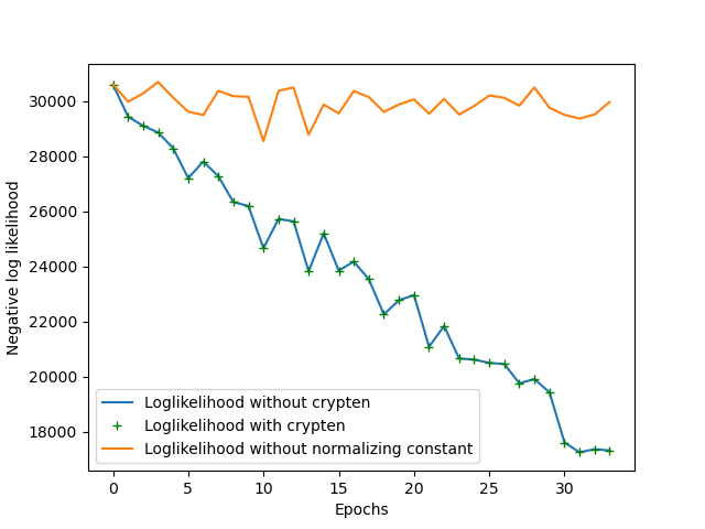
Figure 2: The model learns equally well (error measured as negative log likelihood decreases) with and without the MPC (Crypten). It can be seen that without adding the normalizing constant, the model does not learn, as discussed in Section 4.5.1.

6.3 Evaluation of Algorithm 1

We run the DPVI algorithm used in Jälkö et al., (2017) on the non-partitioned Adult dataset and Algorithm 1 on the vertically partitioned Adult data to assess the effect of fixed point arithmetics to the performance of our inference algorithm.

We can expect some differences between the results from the vertically partitioned DPVI-VPD and the non-partitioned DPVI due to fundamentally different numerical representation used in the algorithm (fixed point in DPVI-VPD vs. floating point in the non-partitioned DPVI). Due to those differences, demonstrating exact equality between the algorithms is not possible, and thus we simply test if the two algorithms converge to equally good local optima.

We run ten repeats of Algorithm 1 with $T=20000$ with minibatches of $100$ data points (i.e., the sampling ratio $q\approx 0.003$). We use the test set negative log-likelihood to measure similarity between the results from the DPVI algorithm with and without vertical partitioning. The algorithm on partitioned data took $\approx 2$-times longer than the algorithm on non-partitioned data (0.4 seconds vs. 0.2 seconds per iteration). Figure 3 shows the negative log-likelihood with the number of epochs evaluated on the test data. We can see that the results are very similar, however, of course, using MPC will increase the run time, and due to fixed point arithmetic, some inaccuracies might arise.

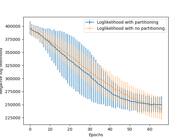
Figure 3: The model learns comparably well (error measured as test-set negative log-likelihood decreases) for DPVI on non-partitioned and vertically partitioned Adult data with 10 repetitions of the algorithm run on 20000 iterations, batch size = 100, and clipping threshold = 1.0. The small differences in the results are due to the discretization for MPC in the partitioned case, while using floating point arithmetics in the non-partitioned case.

7 Discussion

In this paper, we demonstrate the practical feasibility of building privacy-preserving approximate Bayesian inference on vertically partitioned data. We show results on a mixture model with mixture components that factorise across parties. This work easily generalizes to any probabilistic model where the likelihood has no dependence between the different parties.

We can also see that even if some $c\leq P-1$ parties collude to learn more about the data held by the other parties, the algorithm will still guarantee vertically partitioned DP with respect to the parties, however, the collaborating parties now know more about the data. Therefore, with $c\leq P-1$ colluding parties, we can see that Algorithm 1 is $(\epsilon,\delta)$-VPDP with respect to the $P$ parties, such that $\epsilon=\mathcal{O}\left(\delta,Q,T,\mathcal{N}_{\mathbb{Z}/P}\left(0,\frac{(P-c)}{P}\sigma^{2}\right)\right)$ with respect to the $c$ colluding parties, and $\epsilon=\mathcal{O}\left(\delta,Q,T,\mathcal{N}_{\mathbb{Z}/P}\left(0,\frac{(P-1)}{P}\sigma^{2}\right)\right)$ with respect to the non-colluding parties.

One important thing to note is that, if the privacy with respect to the parties is important, sub-sampling might not be a good idea or would need to be kept hidden, since otherwise there is no gain from the sub-sampling amplification.

In this work, we assume the data are matched between the different parties. This is possible if the data contains some identifiers (e.g. a social security number, email address or some other unique identifier) that can be used for matching, although care must be taken to restrict to the matched individuals. Assuming useful identifiers exist, one good option for matching would involve using private set intersection (De Cristofaro and Tsudik,, 2010) for finding the matching records and then sorting them by the identifier to establish a match. This would not reveal any additional information beyond whether a certain individual who exists in the database of one party exists in the database of the other.

If there is no single identifier, the record matching problem becomes more difficult. There exist algorithms for private entity resolution using non-unique identifying information such as names, dates of birth, etc. (Getoor and Machanavajjhala,, 2012; Sehili et al.,, 2015). Using such algorithms increases the possibility of matching errors, which could degrade the performance of the learning. Incorporating such approach into the learning procedure might open interesting possibilities, such as using the data model to help disambiguate uncertain matches.

An obvious next question is what other models could be learned efficiently under this framework. Assuming we are willing to accept slightly larger computational cost, it might be possible to consider models requiring more communication between the parties.

8 Conclusion

We have studied the problem of training a mixture model over vertically partitioned data under DP. Using differential privacy with multiparty computation proved to be non-trivial. Some extra measures were needed in order to train the DP model correctly with vertically partitioned data under MPC.

References

- Abadi et al., (2016) Abadi, M., Chu, A., Goodfellow, I., McMahan, H. B., Mironov, I., Talwar, K., and Zhang, L. (2016). Deep learning with differential privacy. In Proceedings of the 2016 ACM SIGSAC Conference on Computer and Communications Security, pages 308–318, New York, NY, USA. Association for Computing Machinery.
- Acs et al., (2018) Acs, G. et al. (2018). Differentially private mixture of generative neural networks. IEEE Trans. Knowledge and Data Engineering, 31(6):1109–1121.
- Beimel et al., (2010) Beimel, A., Kasiviswanathan, S. P., and Nissim, K. (2010). Bounds on the sample complexity for private learning and private data release. In Theory of Cryptography Conference, pages 437–454. Springer.
- Blum et al., (2008) Blum, A., Ligett, K., and Roth, A. (2008). A learning theory approach to non-interactive database privacy. In Proceedings of the Fortieth Annual ACM Symposium on Theory of Computing, STOC ’08, pages 609–618, New York, NY, USA. ACM.
- Canonne et al., (2020) Canonne, C. L., Kamath, G., and Steinke, T. (2020). The discrete gaussian for differential privacy. Advances in Neural Information Processing Systems, 33:15676–15688.
- Chen et al., (2012) Chen, R., Acs, G., and Castelluccia, C. (2012). Differentially private sequential data publication via variable-length n-grams. In Proceedings of the 2012 ACM conference on Computer and communications security, pages 638–649. ACM.
- Cheon et al., (2017) Cheon, J. H., Kim, A., Kim, M., and Song, Y. (2017). Homomorphic encryption for arithmetic of approximate numbers. In International conference on the theory and application of cryptology and information security, pages 409–437. Springer.
- De Cristofaro and Tsudik, (2010) De Cristofaro, E. and Tsudik, G. (2010). Practical private set intersection protocols with linear complexity. In Sion, R., editor, Financial Cryptography and Data Security, pages 143–159, Berlin, Heidelberg. Springer Berlin Heidelberg.
- Dua and Graff, (2017) Dua, D. and Graff, C. (2017). UCI machine learning repository.
- Dwork et al., (2006) Dwork, C. et al. (2006). Calibrating noise to sensitivity in private data analysis. In Theory of cryptography conf., pages 265–284. Springer.
- Dwork et al., (2009) Dwork, C., Naor, M., Reingold, O., Rothblum, G. N., and Vadhan, S. (2009). On the complexity of differentially private data release: Efficient algorithms and hardness results. In Proceedings of the Forty-first Annual ACM Symposium on Theory of Computing, STOC ’09, pages 381–390, New York, NY, USA. ACM.
- Dwork and Roth, (2014) Dwork, C. and Roth, A. (2014). The algorithmic foundations of differential privacy. Foundations and Trends in Theoretical Computer Science, 9(3–4):211–407.
- Getoor and Machanavajjhala, (2012) Getoor, L. and Machanavajjhala, A. (2012). Entity resolution: theory, practice & open challenges. Proceedings of the VLDB Endowment, 5(12):2018–2019.
- Ghazi et al., (2021) Ghazi, B., Golowich, N., Kumar, R., Manurangsi, P., and Zhang, C. (2021). Deep learning with label differential privacy. Advances in Neural Information Processing Systems, 34:27131–27145.
- Gunning et al., (2019) Gunning, D., Hannun, A., Ibrahim, M., Knott, B., van der Maaten, L., Reis, V., Sengupta, S., Venkataraman, S., and Zhou, X. (2019). CrypTen: A new research tool for secure machine learning with PyTorch.
- Guo et al., (2022) Guo, C., Hannun, A., Knott, B., van der Maaten, L., Tygert, M., and Zhu, R. (2022). Secure multiparty computations in floating-point arithmetic. Information and Inference: A Journal of the IMA, 11(1):103–135.
- Hardt et al., (2012) Hardt, M., Ligett, K., and McSherry, F. (2012). A simple and practical algorithm for differentially private data release. In Advances in Neural Information Processing Systems, pages 2339–2347.
- Jälkö et al., (2017) Jälkö, J., Dikmen, O., and Honkela, A. (2017). Differentially private variational inference for non-conjugate models. In Proceedings of the Thirty-Third Conference on Uncertainty in Artificial Intelligence, UAI 2017, August 11-15, 2017, Sydney, Australia. AUAI Press.
- Jälkö et al., (2021) Jälkö, J., Lagerspetz, E., Haukka, J., Tarkoma, S., Honkela, A., and Kaski, S. (2021). Privacy-preserving data sharing via probabilistic modeling. Patterns, 2(7):100271.
- Jordan et al., (1999) Jordan, M. I., Ghahramani, Z., Jaakkola, T. S., and Saul, L. K. (1999). An introduction to variational methods for graphical models. Machine learning, 37(2):183–233.
- Kairouz et al., (2021) Kairouz, P., Liu, Z., and Steinke, T. (2021). The distributed discrete gaussian mechanism for federated learning with secure aggregation. In International Conference on Machine Learning, pages 5201–5212. PMLR.
- Kairouz et al., (2019) Kairouz, P., McMahan, H. B., Avent, B., Bellet, A., Bennis, M., Bhagoji, A. N., Bonawitz, K., Charles, Z., Cormode, G., Cummings, R., D’Oliveira, R. G. L., Rouayheb, S. E., Evans, D., Gardner, J., Garrett, Z., Gascón, A., Ghazi, B., Gibbons, P. B., Gruteser, M., Harchaoui, Z., He, C., He, L., Huo, Z., Hutchinson, B., Hsu, J., Jaggi, M., Javidi, T., Joshi, G., Khodak, M., Konečný, J., Korolova, A., Koushanfar, F., Koyejo, S., Lepoint, T., Liu, Y., Mittal, P., Mohri, M., Nock, R., Özgür, A., Pagh, R., Raykova, M., Qi, H., Ramage, D., Raskar, R., Song, D., Song, W., Stich, S. U., Sun, Z., Suresh, A. T., Tramèr, F., Vepakomma, P., Wang, J., Xiong, L., Xu, Z., Yang, Q., Yu, F. X., Yu, H., and Zhao, S. (2019). Advances and open problems in federated learning. arXiv:1912.04977.
- Koskela et al., (2020) Koskela, A., Jälkö, J., and Honkela, A. (2020). Computing tight differential privacy guarantees using FFT. volume 108 of Proceedings of Machine Learning Research, pages 2560–2569, Online. PMLR.
- Kucukelbir et al., (2017) Kucukelbir, A., Tran, D., Ranganath, R., Gelman, A., and Blei, D. M. (2017). Automatic differentiation variational inference. The Journal of Machine Learning Research, 18(1):430–474.
- Maurer, (2006) Maurer, U. (2006). Secure multi-party computation made simple. Discrete Applied Mathematics, 154(2):370–381.
- McKenna et al., (2019) McKenna, R., Sheldon, D., and Miklau, G. (2019). Graphical-model based estimation and inference for differential privacy. In Chaudhuri, K. and Salakhutdinov, R., editors, Proceedings of the 36th International Conference on Machine Learning (ICML 2019), volume 97 of Proceedings of Machine Learning Research, pages 4435–4444. PMLR.
- Mironov, (2017) Mironov, I. (2017). Rényi differential privacy. In 2017 IEEE 30th Computer Security Foundations Symposium (CSF), pages 263–275.
- Mohammed et al., (2013) Mohammed, N. et al. (2013). Secure two-party differentially private data release for vertically partitioned data. IEEE trans. on dependable and secure computing, 11(1):59–71.
- Rajkumar and Agarwal, (2012) Rajkumar, A. and Agarwal, S. (2012). A differentially private stochastic gradient descent algorithm for multiparty classification. In Proc. AISTATS 2012, pages 933–941.
- Rubin, (1993) Rubin, D. B. (1993). Statistical disclosure limitation. Journal of official Statistics, 9(2):461–468.
- Samarati and Sweeney, (1998) Samarati, P. and Sweeney, L. (1998). Generalizing data to provide anonymity when disclosing information. In PODS, pages 10–1145.
- Sehili et al., (2015) Sehili, Z., Kolb, L., Borgs, C., Schnell, R., and Rahm, E. (2015). Privacy preserving record linkage with PPJoin. Datenbanksysteme für Business, Technologie und Web (BTW 2015).
- Shamir, (1979) Shamir, A. (1979). How to share a secret. Communications of the ACM, 22(11):612–613.
- Sommer et al., (2019) Sommer, D. M., Meiser, S., and Mohammadi, E. (2019). Privacy loss classes: The central limit theorem in differential privacy. Proceedings on Privacy Enhancing Technologies, 2019(2):245–269.
- Song et al., (2013) Song, S., Chaudhuri, K., and Sarwate, A. D. (2013). Stochastic gradient descent with differentially private updates. In Proc. GlobalSIP 2013, pages 245–248.
- Sweeney, (2002) Sweeney, L. (2002). k-anonymity: A model for protecting privacy. International journal of uncertainty, fuzziness and knowledge-based systems, 10(05):557–570.
- Titsias and Lázaro-Gredilla, (2014) Titsias, M. and Lázaro-Gredilla, M. (2014). Doubly stochastic variational Bayes for non-conjugate inference. In International conference on machine learning, pages 1971–1979.
- Wang et al., (2020) Wang, C., Liang, J., Huang, M., Bai, B., Bai, K., and Li, H. (2020). Hybrid differentially private federated learning on vertically partitioned data. arXiv preprint arXiv:2009.02763.
- Xiao et al., (2010) Xiao, Y., Xiong, L., and Yuan, C. (2010). Differentially private data release through multidimensional partitioning. In Workshop on Secure Data Management, pages 150–168. Springer.
- Yao, (1982) Yao, A. C. (1982). Protocols for secure computations. In 23rd Annual Symposium on Foundations of Computer Science (SFCS 1982), pages 160–164. IEEE.
- Yoon et al., (2019) Yoon, J., Jordon, J., and van der Schaar, M. (2019). PATE-GAN: Generating synthetic data with differential privacy guarantees. In International Conference on Learning Representations (ICLR 2019).
- Zhang et al., (2014) Zhang, J., Cormode, G., Procopiuc, C. M., Srivastava, D., and Xiao, X. (2014). PrivBayes: Private data release via Bayesian networks. In Proceedings of the 2014 ACM SIGMOD International Conference on Management of Data, SIGMOD ’14, pages 1423–1434, New York, NY, USA. ACM.