Characterizing the First-Arriving Multipath
Component in 5G Millimeter Wave Networks:
TOA, AOA, and Non-Line-of-Sight Bias

Abstract

This paper presents a stochastic geometry-based analysis of propagation statistics for 5G millimeter wave (mm-wave) cellular. In particular, the time-of-arrival (TOA) and angle-of-arrival (AOA) distributions of the first-arriving multipath component (MPC) are derived. These statistics find their utility in many applications such as cellular-based localization, channel modeling, and link establishment for mm-wave initial access (IA). Leveraging tools from stochastic geometry, a Boolean model is used to statistically characterize the random locations, orientations, and sizes of reflectors, e.g., buildings. Assuming non-line-of-sight (NLOS) propagation is due to first-order (i.e., single-bounce) reflections, and that reflectors can either facilitate or block reflections, the distribution of the path length (i.e., absolute time delay) of the first-arriving MPC is derived. This result is then used to obtain the first NLOS bias distribution in the localization literature that is based on the absolute delay of the first-arriving MPC for outdoor time-of-flight (TOF) range measurements. This distribution is shown to match exceptionally well with commonly assumed gamma and exponential NLOS bias models in the literature, which were only attained previously through heuristic or indirect methods. Continuing under this analytical framework, the AOA distribution of the first-arriving MPC is derived, which gives novel insight into how environmental obstacles affect the AOA and also represents the first AOA distribution derived under the Boolean model.

I Introduction

The past decade has seen tremendous advances in both the understanding and characterization of the mm-wave channel for 5G cellular. These advances have been realized, in part, by the development of stochastic geometry-based analytical models. One of the most tractable stochastic geometry tools employed to study mm-wave propagation, and consequently the most widely-utilized, is that of the Boolean model, which is able to statistically capture the randomness in the locations, sizes, and orientations of environmental obstacles (e.g., buildings) [2]. The pioneering work first utilizing the Boolean model to study mm-wave propagation in cellular networks was conducted in [3]. While an excellent examination of the Boolean model’s usefulness in studying blockage effects, the analysis in [3] was focused on line-of-sight (LOS) links, and thus, the study of NLOS propagation under this model remained an open problem.

An important aspect of mm-waves is that diffraction effects are negligible while reflections dominate NLOS propagation [4]. Thus, while [3] did not study multipath effects under the Boolean model, other subsequent works have. In [5] for example, first-order reflections were incorporated into the Boolean model to derive the power delay profile (PDP). The work in [6] extends that of [5] by considering buildings with random orientations and equipping the transmitter (Tx) and receiver (Rx) with directional antennas. Channel characteristics were then derived under first-order reflections and independent blocking. In [7], the Boolean model under first-order reflections and independent blocking was used, along with a point process of transmitters, to “quantify the total amount of network interference.” Lastly, the work in [8] also utilized a similar model to derive the probability an anchor-mobile pair can perform single-anchor localization.

While many works incorporate NLOS propagation into the Boolean model, including the ones above, they unfortunately either have restrictive setups or they do not derive our metrics of interest, namely, the TOA and AOA statistics of the first-arriving MPC experienced at the mobile for a single link. For example, the model in [5] does not consider random orientations of buildings in a given Boolean model realization, and in [6], the assumption of directional antennas pointed in fixed directions makes it difficult to determine whether other NLOS paths are available from different directions. Finally, while [9] does find the TOA of the first-arriving MPC, the model assumes one-dimensional reflectors and only the reflector closest to the mobile is responsible for facilitating the first-arriving reflection, an assumption that does not often hold.

The obvious next question is: Why are the TOA and AOA statistics of the first-arriving MPC important? We begin with the TOA. In addition to its use in establishing an absolute timing reference for channel modeling purposes, the TOA distribution of the first-arriving MPC is perhaps most useful for addressing the NLOS bias problem that arises in localization. The NLOS bias problem can be summarized as follows. Consider a range measurement where the distance between a base station and a mobile is measured via the TOF of a signal transmitted by either node. In a LOS scenario, multiplying the TOF by the speed of light yields the true base station-mobile separation distance. However, the LOS path is often blocked and the resulting reflected, diffracted, or scattered signal will lead to an erroneously larger range estimate than the true separation distance. This distance the signal travels in excess of the true LOS distance is termed the NLOS bias. When these positively biased range measurements are used to perform localization, they ultimately lead to a biased/poor target position estimate.

For a noiseless NLOS, TOF range measurement, the range and bias are related simply by:

$$R=d+B,$$ (1)

where $R$ is the distance (i.e., range) measured via the TOF, $d$ is the true separation distance, and $B$ is the NLOS bias ($P[B>0]=1$) [10]. In many NLOS localization algorithms and analyses, having a priori information regarding the statistics of the bias error (e.g., the distribution of $B$ in (1)) can improve NLOS detection [11], improve estimator performance [12], and reduce the Cramér-Rao Lower Bound on positioning error as well [13]. Thus, obtaining an accurate distribution of the NLOS bias is of vital importance for geolocation in NLOS environments.

Although the NLOS bias problem has been around since the inception of range-based localization, there are, at present, no agreed upon statistical distributions characterizing the bias error in outdoor environments, such as urban canyons (see Sec. III-C). While the localization literature does offer a variety of bias distributions, they are either: 1) chosen simply due to their tractability or desirable features such as having a positive support, e.g., half-Gaussian [14], Rayleigh [15], positive uniform [16], and gamma [17]; 2) chosen based on simple point scattering models from the channel modeling literature [13, Sec. III-B], [18], [19]; or 3) chosen indirectly based on the delay of the first-arriving MPC from empirical excess delay LOS PDP models, such as the commonly used exponential distribution [20], [21], and not directly via the first-arriving MPC from absolute delay NLOS PDPs. Since range measurements are often triggered on the first-arriving signal [13], [22], then if the LOS path is blocked, the first-arriving MPC (i.e., the first-arriving reflection assumed here) will be responsible for triggering the range measurement. Thus, in an NLOS scenario, obtaining the absolute delay (i.e., TOA or path length) distribution of the first-arriving MPC will yield the distribution of the range measurement, and subtracting from this the true base station-mobile separation distance will yield the distribution of the NLOS bias via (1). Unfortunately, obtaining this TOA distribution empirically, through an outdoor measurement campaign, is a difficult task (see Sec. III-C). Thus, an accurate analytical solution is needed. Towards this end, this paper derives the TOA distribution of the first-arriving MPC under the Boolean model, which characterizes the TOA over all random placements of environmental obstacles. This result then yields the NLOS bias distribution; thus filling the void in the localization literature by offering the first bias distribution derived via the absolute delay of the first-arriving MPC and under a comprehensive stochastic geometry framework.

We now address the AOA. As mm-waves “generally require high directionality to achieve a sufficient signal-to-noise-ratio (SNR),” beam sweeping, a process whereby angular sections are tested and checked for a received signal, will be needed to establish links in the IA phase [23]. Since the first-arriving MPC is often likely to be the dominant MPC, understanding its AOA distribution will be important for developing techniques to improve the angular search space in the IA phase; reducing the time it takes to close a link. Thus, this paper also derives the AOA distribution of the first-arriving MPC, which is the first AOA distribution derived under the Boolean model. Additionally, this AOA distribution offers a distinct advantage over AOA distributions derived under older omni-directional scattering models, e.g., [18], [24], since point scatters can not capture blocking effects nor the dominant reflection effects of mm-waves.

Given the gaps in the stochastic geometry and localization literature, our contributions are:

1. The derivation of the TOA distribution of the first-arriving MPC under the Boolean model, both with and without blocking, which yields the NLOS bias distribution.

2. An analysis highlighting the close connection between this NLOS bias distribution and the exponential and gamma bias model assumptions in the localization literature.

3. A discussion regarding the lack of outdoor measurement data characterizing NLOS bias and what information about the bias can be gleaned from measurements that do exist.

4. The derivation of the AOA distribution of the first-arriving MPC under the Boolean model, which represents the first AOA distribution derived under the Boolean model.

5. A numerical analysis of this distribution which reveals the connection between this AOA distribution and that derived under an elliptical, omni-directional scattering model.

II System Model

This section first introduces the system model assumptions and then describes the Boolean model setup. Next, a characterization of first-order reflections is given followed by a description of independent blocking. Finally, an important result is presented regarding the number of reflectors facilitating visible (non-blocked) reflections. Common notation is given in Table I.

II-A Assumptions

Assumption 1 (NLOS Propagation).

Only first-order specular reflections are considered.

Remark.

First, specular reflections imply the angle-of-incidence (AOI) equals angle-of-reflection (AOR) at the point of incidence. Second, the effects of higher-order (i.e. multiple-bounce) reflections are considered to be minimal due to increased pathloss and reflection losses, e.g., see [5] and [6]. Third, diffraction effects are negligible at mm-wave frequencies [4] and hence are not considered. Lastly, assuming only specular reflections implies that reflecting surfaces are sufficiently smooth such that scattering effects are negligible as well [5], [25].

Assumption 2 (360$\degree$ Coverage).

The base station and mobile are equipped with either isotropic antennas or antenna arrays allowing 360$\degree$ beam sweeping, i.e., all reflection paths are illuminated.

Assumption 3 (Independent Blocking).

Blocking on each received signal path is assumed to be independent. Further, for each reflection, blocking on the incident path is assumed to be independent of blocking on the reflected path.

Remark.

Treating blocking on each received signal path independently, i.e., independent blocking, is a common assumption in the literature [5], [6], [7]. Further, for each separate reflection path, treating blocking independently on the incident and reflected paths has been done previously in [8], and a similar treatment is also presented in [26]. Sections III-B and IV-A reveal that treating the incident and reflected paths independently matches true correlated blocking rather well.

Remark.

Since blocking is independent on each received path, then blocking on the LOS path between the base station and mobile does not impact blocking on reflected paths. Thus, whether the LOS path is blocked or not does not impact the analysis. As such, we simply assume the LOS path is blocked for the NLOS bias analysis and can also simply ignore whether the LOS path is blocked or not in the AOA analysis. This is explored further in Sections III-B and IV.

TABLE I: Summary of Notation

Symbol	Description	Symbol	Description
$f_{X}(\cdot)$	Probability distribution fn. (PDF) of RV $X$	$F_{X}(\cdot)$	Cumulative distribution fn. (CDF) of RV $X$
$\textbf{Supp}(X)$	Support of the RV $X$: $\{x\in\mathbb{R}\,|\,f_{X}(x)>0\}$	$\mathbb{E}[X]$	Expectation of the RV $X$
$P[A]$	Probability of event $A$	$\lVert\cdot\rVert$	The Euclidean norm
$\delta(\cdot)$	The Dirac delta function	$\mathbbm{1}[A]$	Indicator Function, 1 if A true, 0 if A false
$\mathbf{x}$	Vector $\mathbf{x}$. All vectors are column vectors.	$[\mathbf{x}]_{i}$; $\mathbf{x}\cdot\mathbf{y}$	$i^{\text{th}}$ component of $\mathbf{x}$; Dot product of $\mathbf{x}$ with $\mathbf{y}$
$\mathbf{g}(x)$; $g(\mathbf{x})$	Vector fn. of a scalar; Scalar fn. of a vector	$\mathbf{X}^{T}$; $\mathbf{X}^{-1}$	Transpose of matrix $\mathbf{X}$; Inverse of matrix $\mathbf{X}$
$\mathbf{g}(\mathbf{x})$; $g(x)$	Vector fn. of a vector; Scalar fn. of a scalar	$\mathbf{R}_{\theta}$	The rotation matrix $\Bigl{[}\begin{smallmatrix}\cos\theta&\sin\theta\\ -\sin\theta&\cos\theta\end{smallmatrix}\Bigr{]}$ which
$\mathcal{L}_{[\mathbf{p},\mathbf{q}]}$	The set of points forming a line segment		rotates a vector clockwise by angle $\theta$
	between, and including, the points $\mathbf{p}$ and $\mathbf{q}$	$\mathcal{Q}$; $\varnothing$	Roman numeral set:$\{\text{I},\text{II},\text{III},\text{IV}\}$; Empty set
$\mu_{n}\big{(}\mathcal{A}\big{)}$	The $n$-dim. Lebesgue measure of set $\mathcal{A}$	$\partial\mathcal{A}$	Boundary of set $\mathcal{A}$ (closure minus interior)
$\Phi$	Set of points forming a Poisson Pt. Proc.	$\Phi(\mathcal{A})$	The number of points of $\Phi$ in the set $\mathcal{A}$
$\mathcal{A}\oplus\mathcal{B}$	Minkowski sum: For compact $\mathcal{A},\mathcal{B}\subset\mathbb{R}^{2}$,	$\mathcal{A}\setminus\mathcal{B}$	Set subtraction: $\{\mathbf{x}\in\mathcal{A}\,|\,\mathbf{x}\notin\mathcal{B}\}$
	$\mathcal{A}\oplus\mathcal{B}\triangleq\big{\{}\mathbf{x}+\mathbf{y}\in\mathbb{R}^{2}\,\big{|}\,\mathbf{x}\in\mathcal{A},\mathbf{y}\in\mathcal{B}\big{\}}$	$Q_{\text{I}}$	$1^{\text{st}}$ quadrant in $\mathbb{R}^{2}$:$\Big{\{}\,\![x,y]^{T}\!\!\!\in\mathbb{R}^{2}\!\;\Big{|}\;\!x\!\geq\!0,y\!\geq\!0\!\,\Big{\}}$
w.l.o.g.; s.t.	Without loss of generality; such that		Remaining quad.’s defined similarly.
l.h.s.; r.h.s.	Left hand side; right hand side	c.c.w.; w.r.t.	Counterclockwise; with respect to

II-B Reflection Fundamentals Under the Boolean Model

This section first introduces the Boolean model setup and then uses this setup, along with the assumptions above, to derive results regarding first-order reflections. We begin by formally defining our use of the term reflector.

Definition 1 (Reflector $\mathcal{R}_{w,\theta,\mathbf{c}}$).

A reflector $\mathcal{R}_{w,\theta,\mathbf{c}}$ is defined to be a square compact set with edge width $w\in(0,\infty)$, center point $\mathbf{c}\in\mathbb{R}^{2}$, and orientation $\theta\in(0,\pi/2)$, measured c.c.w. w.r.t. the $+x$-axis. To aid in the analysis, we further define four internal vectors, $\mathbf{k}_{\text{I}},\mathbf{k}_{\text{II}},\mathbf{k}_{\text{III}},\mathbf{k}_{\text{IV}}$, which are depicted in Fig. 1, and of which $\mathbf{k}_{\text{III}}$ exhibits the reflector’s orientation, $\theta$.

Remark.

Although the term reflector is used, a reflector $\mathcal{R}_{w,\theta,\mathbf{c}}$ can both facilitate a reflection and/or act as an impenetrable blockage.

Definition 2 (Boolean Model of Reflectors, $\mathcal{B}$).

Let $\Phi=\{\mathbf{c}_{i}\}_{i=1}^{\infty}$ be a homogeneous PPP over $\mathbb{R}^{2}$ with intensity $\lambda>0$, let $\mathcal{U}=\{W_{i}\}_{i=1}^{\infty}$, $\mathcal{V}=\{\Theta_{i}\}_{i=1}^{\infty}$ be sequences of RVs representing the widths and orientations of reflectors, respectively, and let $\mathcal{U},\mathcal{V}$, and $\Phi$ be mutually independent. Next, let $\{W_{i}\}_{i=1}^{\infty}\!\mathbin{\overset{\text{\scriptsize i.i.d.}}{\kern 0.0pt\leavevmode\resizebox{13.61111pt}{3.66875pt}{$\sim$}}}\!f_{W}(w)$ and $\{\Theta_{i}\}_{i=1}^{\infty}\!\mathbin{\overset{\text{\scriptsize i.i.d.}}{\kern 0.0pt\leavevmode\resizebox{13.61111pt}{3.66875pt}{$\sim$}}}\!f_{\Theta}(\theta)$, where $f_{W}=\text{unif}(w_{min},w_{max},n_{w})$ and $f_{\Theta}=\text{unif}(\theta_{min},\theta_{max},n_{\theta})$. Then, the Boolean model of reflectors is defined as: $\mathcal{B}\triangleq\bigcup_{i=1}^{\infty}\,\mathcal{R}_{W_{i},\Theta_{i},\mathbf{c}_{i}}$.

Remark.

Note, $\mathcal{B}$ is a random set in $\mathbb{R}^{2}$. A realization of $\mathcal{B}$ is given when the widths, $\{W_{i}\}_{i=1}^{\infty}$, orientations, $\{\Theta_{i}\}_{i=1}^{\infty}$, and the PPP of center points, $\Phi$, are sampled according to the rules above. We use ‘$\mathcal{B}$’ for both the random set and its realization. Its usage will be clear from context.

Definition 3 (Test Link).

The test link setup is defined to be that which places the base station at $\mathbf{b}\triangleq\big{[}-d/2,0\big{]}^{T}$ and the mobile at $\mathbf{m}\triangleq\big{[}d/2,0\big{]}^{T}$, for $d>0$. (See Fig. 1.)

Remark.

The results derived in this paper apply w.l.o.g. to any translation and/or orientation of this test link setup due to the stationary and isotropic properties of the Boolean model [2].

Figure 1: System Model. Depicted is a realization of the Boolean model over the test link setup, along with illustrations of various concepts and definitions from Sec. II such as: correlated blocking, independent blocking, reflection point characteristics, and a reflector’s internal vectors. The path length of the first-arriving reflection is $S_{(1)}=s_{(1)}$ and its AOA is $A_{(1)}=\alpha_{(1)}$.

This Boolean model setup, along with Assumptions 1 and 2, leads to some important geometric consequences regarding first-order reflections, which we now summarize. We begin by considering a single reflector, $\mathcal{R}_{w,\theta,\mathbf{c}}$, with fixed width and orientation, yet arbitrary center point. Next, let $\mathbf{r}\in\mathbb{R}^{2}$. We say that $\mathbf{r}$ is a potential reflection point (PRP) for $\mathcal{R}_{w,\theta,\mathbf{c}}$ if $\mathcal{R}_{w,\theta,\mathbf{c}}$ can be placed s.t. an edge of $\mathcal{R}_{w,\theta,\mathbf{c}}$ can intersect $\mathbf{r}$ to establish a first-order reflection at $\mathbf{r}$ (i.e., AOI$\,=\,$AOR at $\mathbf{r}$). The following lemma lists all of the PRPs for $\mathcal{R}_{w,\theta,\mathbf{c}}$.

Lemma 1 (Reflection Hyperbola).

Let $\mathcal{H}_{\theta}$ be the set of all PRPs for reflector $\mathcal{R}_{w,\theta,\mathbf{c}}$. Then,

$$\mathcal{H}_{\theta}=\Big{\{}[x,y]^{T}\!\!\in\mathbb{R}^{2}~{}\Big{|}~{}y^{2}-x^{2}+2\cot(2\theta)xy+d^{2}/4=0\Big{\}}.$$ (2)

Proof.

First, note that $\mathbf{b}$ and $\mathbf{m}$ are always considered to be PRPs regardless of the reflector orientation, and thus trivially satisfy the lemma. Next, we prove forward and reverse containment.

($\subset$): Let $\mathbf{r}=[x,y]^{T}\!\in\mathcal{H}_{\theta}/\{\mathbf{b},\mathbf{m}\}$. Then $\theta\in(0,\pi/2)\!\implies\!\exists!\,q\in\mathcal{Q}$ s.t. $\mathbf{r}\in Q_{q}$. Next, let the vectors $\mathbf{r}-\mathbf{b}$ and $\mathbf{m}-\mathbf{r}$ represent the incident and reflected paths, respectively. The AOI and AOR at $\mathbf{r}$ are given by

$$~{}~{}~{}~{}~{}~{}~{}~{}~{}~{}~{}~{}~{}~{}~{}~{}\varphi_{I}\triangleq\cos^{-1}\!\Bigg{(}\frac{\mathbf{k}_{q}\cdot(\mathbf{b}-\mathbf{r})}{\lVert\mathbf{k}_{q}\rVert\lVert\mathbf{b}-\mathbf{r}\rVert}\Bigg{)}~{}~{}~{}~{}\text{and}~{}~{}~{}~{}\varphi_{R}\triangleq\cos^{-1}\!\Bigg{(}\frac{\mathbf{k}_{q}\cdot(\mathbf{m}-\mathbf{r})}{\lVert\mathbf{k}_{q}\rVert\lVert\mathbf{m}-\mathbf{r}\rVert}\Bigg{)},~{}~{}~{}~{}~{}~{}(\text{see Fig. \ref{System_Model_Fig}})$$

which are both measured w.r.t. the vector, $\mathbf{k}_{q}$, where $\mathbf{k}_{q}$ is normal to the edge that would facilitate the reflection in $Q_{q}$. Since $\mathbf{r}$ is a PRP by implication, then $\varphi_{I}=\varphi_{R}$, and upon simplification, we have that for any $q\in\mathcal{Q}$, $y^{2}-x^{2}+2\cot(2\theta)xy+d^{2}/4=0$. Thus, $\mathbf{r}$ is in the r.h.s. of (2).

($\supset$): Let $\mathbf{r}=[x,y]^{T}$ satisfy the r.h.s. of (2), where $\mathbf{r}\neq\mathbf{b},\mathbf{m}$ (these are already PRPs). Since $\mathbf{b}$ and $\mathbf{m}$ are the only points on the $x$, $y$ axes that are in the r.h.s. of (2), then $\exists!q\in\mathcal{Q}$ s.t. $\mathbf{r}\in Q_{q}$, where $\mathbf{r}$ satisfies $y^{2}-x^{2}+2\cot(2\theta)xy+d^{2}/4=0$. For any $q$, we can work backwards from this equation to establish: $\frac{\mathbf{k}_{q}\cdot(\mathbf{b}-\mathbf{r})}{\lVert\mathbf{k}_{q}\rVert\lVert\mathbf{b}-\mathbf{r}\rVert}=\frac{\mathbf{k}_{q}\cdot(\mathbf{m}-\mathbf{r})}{\lVert\mathbf{k}_{q}\rVert\lVert\mathbf{m}-\mathbf{r}\rVert}$. This implies $\varphi_{I}=\varphi_{R}$ at $\mathbf{r}$ and hence $\mathbf{r}\in\mathcal{H}_{\theta}$. ∎

Remark.

Note the following: 1) For $\mathbf{r}\in\mathbb{R}^{2}$, $\mathbf{r}$ is a PRP for $\mathcal{R}_{w,\theta,\mathbf{c}}$ if and only if $\mathbf{r}\in\mathcal{H}_{\theta}$; 2) the set condition in (2) is a hyperbola, and thus we refer to the set of PRPs for $\mathcal{R}_{w,\theta,\mathbf{c}}$ as the reflection hyperbola for $\mathcal{R}_{w,\theta,\mathbf{c}}$; 3) the reflector orientation, $\theta$, is only present in the “$xy$” term of the hyperbola equation, which implies that changing the orientation of the reflector results in a rotation of this hyperbola about the origin. See Fig. 2 for an example of $\mathcal{H}_{\theta=\pi/3}$.

Remark.

Indeed, a reflector $\mathcal{R}_{w,\theta,\mathbf{c}}$ has uncountably many PRPs. If $\mathcal{R}_{w,\theta,\mathbf{c}}$ were to actually intersect one of these PRPs with the appropriate edge, then a reflection would be established. We would then refer to this particular PRP as the reflection point (RP). Thus, $\mathcal{R}_{w,\theta,\mathbf{c}}$ has many PRPs but can have only one RP. Since this lemma states that all PRPs for $\mathcal{R}_{w,\theta,\mathbf{c}}$ lie on $\mathcal{H}_{\theta}$, then to check whether $\mathcal{R}_{w,\theta,\mathbf{c}}$ generates a reflection, one simply needs to check whether the appropriate edge of $\mathcal{R}_{w,\theta,\mathbf{c}}$ intersects the reflection hyperbola.

We are oftentimes interested in reflection points corresponding to reflection paths less than or equal to a certain distance, $s$. The terminology below aids in this characterization.

Definition 4 (The $s$-Ellipse).

Under the test link setup, the s-ellipse is defined as: $\mathcal{P}_{s}\triangleq\Big{\{}[x,y]^{T}\in\mathbb{R}^{2}~{}\Big{|}~{}x^{2}\big{/}u^{2}+y^{2}\big{/}v^{2}\leq 1\Big{\}}$, where $u^{2}=s^{2}/4$, $v^{2}=(s^{2}-d^{2})/4$, and $d<s<\infty$. Further, for $s=d$ we set $\mathcal{P}_{d}\triangleq\lim_{s\to d}\mathcal{P}_{s}=\mathcal{L}_{[\mathbf{b},\mathbf{m}]}$, and for $s=\infty$, we set $\mathcal{P}_{\infty}\triangleq\lim_{s\to\infty}\mathcal{P}_{s}=\mathbb{R}^{2}$. (See Fig. 2.)

Lastly, four PRPs exist which $\mathcal{R}_{w,\theta,\mathbf{c}}$ can intersect to generate reflections of exactly $s$ meters.

Lemma 2 (Boundary PRPs).

Let $d\leq s<\infty$. Consider the test link setup, a reflector $\mathcal{R}_{w,\theta,\mathbf{c}}$, and its corresponding reflection hyperbola, $\mathcal{H}_{\theta}$. Then, $(\mathcal{H}_{\theta}\cap\partial\mathcal{P}_{s})=\big{\{}\mathbf{h}_{\text{\emph{I}}},\mathbf{h}_{\text{\emph{II}}},\mathbf{h}_{\text{\emph{III}}},\mathbf{h}_{\text{\emph{IV}}}\big{\}}$, where

$$\mathbf{h}_{\text{\emph{I}}}=\bigg{[}\!\sqrt{z_{\text{\emph{I, III}}}}~{}\!,\frac{v}{u}\sqrt{u^{2}-\!z_{\text{\emph{I,III}}}}\bigg{]}^{T}\!,~{}\mathbf{h}_{\text{\emph{II}}}=\bigg{[}\!-\!\sqrt{z_{\text{\emph{II, IV}}}}~{}\!,\frac{v}{u}\sqrt{u^{2}-\!z_{\text{\emph{II,IV}}}}\bigg{]}^{T}\!\!,~{}~{}\mathbf{h}_{\text{\emph{III}}}=-\mathbf{h}_{\text{\emph{I}}},~{}~{}\mathbf{h}_{\text{\emph{IV}}}=-\mathbf{h}_{\text{\emph{II}}},~{}~{}~{}\text{and}$$

$$z_{\text{\emph{I, III}}}=\frac{s^{4}\cot^{2}\!\theta}{4\Big{[}s^{2}\csc^{2}\!\theta-d^{2}\Big{]}},~{}~{}z_{\text{\emph{II, IV}}}=\frac{s^{4}\tan^{2}\!\theta}{4\Big{[}s^{2}\sec^{2}\!\theta-d^{2}\Big{]}}.$$

The variables $u$ and $v$ are from Definition 4. (See Fig. 2 for a depiction of these points.)

Proof.

Solve the system of two equations that define $\mathcal{H}_{\theta}$ and $\partial\mathcal{P}_{s}$. ∎

Remark.

The $\mathbf{h}_{q}$’s are functions of $s$, $d$, and $\theta$. We write ‘$\mathbf{h}_{q}(s)$’ to highlight the dependency on $s$, omit writing the dependency on $d$, and occasionally use a subscript $\theta$ to remind the reader when necessary. The Roman numeral subscript on the $\mathbf{h}_{q}$’s denotes the quadrant in which it resides, for $s>d$. For $s=d$, these points simplify to $\mathbf{b}$ and $\mathbf{m}$. For $s=\infty$ not stated in the lemma, we set $\mathbf{h}_{q}(\infty)\triangleq\lim_{s\to\infty}\mathbf{h}_{q}(s)=[\pm\infty,\pm\infty]^{T}$, $\forall q\in\mathcal{Q}$, where ‘$\pm$’ depends on the quadrant.

II-C Blocking

This section briefly discusses what it means for a reflection point to be visible, i.e., non-blocked under Assumption 3 (independent blocking). As this treatment is analogous to that in [8], we only summarize the relevant results here, without proof.

Definition 5 (Visible Reflection Point (VRP) for $\mathcal{R}_{w,\theta,\mathbf{c}}$).

Let $\mathcal{B}$, $\mathcal{B}_{1}$, and $\mathcal{B}_{2}$ be realizations of i.i.d. Boolean models and let $\mathbf{r}\in\mathbb{R}^{2}$ be a RP for $\mathcal{R}_{w,\theta,\mathbf{c}}\subset\mathcal{B}$. Then, the reflection path through $\mathbf{r}$ is visible if $(\mathcal{B}_{1}\cap\mathcal{L}_{[\mathbf{b},\mathbf{r}]})\cup(\mathcal{B}_{2}\cap\mathcal{L}_{[\mathbf{r},\mathbf{m}]})=\varnothing$. In this case, we say $\mathbf{r}$ is a visible RP for $\mathcal{R}_{w,\theta,\mathbf{c}}$.

Remark.

As a simple example, if $\mathcal{B}$, $\mathcal{B}_{1}$, and $\mathcal{B}_{2}$ only contain reflectors of width $w^{\prime}$ and orientation $\theta^{\prime}$, then RP $\mathbf{r}^{\prime}$ in Fig. 1 is visible if no reflector center point from $\mathcal{B}_{1}$ falls in: $\mathcal{L}_{[\mathbf{b},\mathbf{r}^{\prime}]}\oplus\mathcal{R}_{w^{\prime},\theta^{\prime},\mathbf{0}}$, and no reflector center point from $\mathcal{B}_{2}$ falls in: $\mathcal{L}_{[\mathbf{r}^{\prime},\mathbf{m}]}\oplus\mathcal{R}_{w^{\prime},\theta^{\prime},\mathbf{0}}$. When $\mathcal{B}$, $\mathcal{B}_{1}$, and $\mathcal{B}_{2}$ contain reflectors of many widths and orientations, the probability a RP is visible is given below.

Lemma 3 (Probability a Reflection Point is Visible [8]).

Consider the test link setup and let $\mathcal{B}$, $\mathcal{B}_{1}$, and $\mathcal{B}_{2}$ be i.i.d. Boolean models and $\mathbf{r}\in\mathbb{R}^{2}$ be a reflection point for $\mathcal{R}_{w,\theta,\mathbf{c}}\subset\mathcal{B}$. Then, the probability that $\mathbf{r}$ is a VRP for $\mathcal{R}_{w,\theta,\mathbf{c}}$ is given by

$$\rho(\mathbf{r}) =P\big{[}(\mathcal{B}_{1}\cap\mathcal{L}_{[\mathbf{b},\mathbf{r}]})\cup(\mathcal{B}_{2}\cap\mathcal{L}_{[\mathbf{r},\mathbf{m}]})=\varnothing\big{]}=e^{-\lambda\mathbb{E}_{W,\Theta}\Big{[}\mu_{2}\big{(}\mathcal{L}_{[\mathbf{b},\mathbf{r}]}\oplus\mathcal{R}_{W,\Theta,\mathbf{0}}\big{)}+\mu_{2}\big{(}\mathcal{L}_{[\mathbf{r},\mathbf{m}]}\oplus\mathcal{R}_{W,\Theta,\mathbf{0}}\big{)}\Big{]}},$$

where $\forall\mathbf{p},\mathbf{q}\in\mathbb{R}^{2}$, $\mathbf{p}\neq\mathbf{q}$

$$\mu_{2}\big{(}\mathcal{L}_{[\mathbf{p},\mathbf{q}]}\oplus\mathcal{R}_{w,\theta,\mathbf{0}}\big{)}=\begin{cases}\sqrt{2}\,w\lVert\mathbf{p}-\mathbf{q}\rVert\,\sin\big{(}\pi/4+\theta-\eta\big{)}+w^{2},&0\leq\theta-\eta\leq\pi/2\\[-1.72218pt] \sqrt{2}\,w\lVert\mathbf{p}-\mathbf{q}\rVert\,\big{|}\sin\big{(}\!-\pi/4+\theta-\eta\big{)}\big{|}+w^{2},&\text{\emph{otherwise}}\\[-5.16663pt] \end{cases},\vspace{-3pt}$$

and $\eta=\tan^{-1}\big{[}([\mathbf{q}]_{2}-[\mathbf{p}]_{2})/([\mathbf{q}]_{1}-[\mathbf{p}]_{1})\big{]}$, and for $\mathbf{p}=\mathbf{q}$, $\mu_{2}\big{(}\mathcal{L}_{[\mathbf{p},\mathbf{q}]}\oplus\mathcal{R}_{w,\theta,\mathbf{0}}\big{)}=w^{2}$.

Proof.

Please refer to [8]. Note that the interplay between the slope of the line segment $\mathcal{L}_{[\mathbf{p},\mathbf{q}]}$, given by $\eta$, and the orientation of the reflector, $\theta$, is what dictates how the Lebesgue measure of ‘$\mathcal{L}_{[\mathbf{p},\mathbf{q}]}\oplus\mathcal{R}_{w,\theta}$’ is evaluated – hence the piecewise function. ∎

II-D The Number of Reflectors Producing Visible Reflections

Considering reflections with path lengths between $s_{1}$ and $s_{2}$ meters, this section presents the number of reflectors producing visible reflections, denoted by the RV: $V_{[s_{1},\,s_{2}]}$, where $d\leq s_{1}\leq s_{2}\leq\infty$. A subset of this metric, namely $V_{[d,s_{2}]}$ for $d=s_{1}\leq s_{2}<\infty$, was also studied in [8] in the context of single-anchor localization. However, the general metric is of particular interest to us here for two reasons. The first is that it considers the infinite case, i.e., $V_{[d,\,\infty]}$, which is vitally important in the derivations that follow since this gives the total number of reflectors producing visible reflections on all of $\mathbb{R}^{2}$. Obtaining this infinite case requires proving extra convergence results (Appendix A). The second is that restricting our attention to reflections of distances $[s_{1},\,s_{2}]$ aids in the derivation of the AOA. Below we present the lemma for the general metric, $V_{[s_{1},s_{2}]}$. With the exception of the infinite case, the method behind the derivation is similar to that presented in [8]. Thus, we only provide a proof sketch here to connect system model concepts to the analysis which follows and to give insight needed for subsequent derivations.

Figure 2: Analytical Framework. The gray region in $Q_{\text{I}}$ is the region where the endpoint of $\mathbf{k}_{\text{I}}$ of reflector $\mathcal{R}_{w_{i},\theta_{j},\mathbf{c}}$ (see Fig. 1) can lie in order to produce a first order reflection between $\mathbf{b}$ and $\mathbf{m}$ of distance in $[s_{1},s_{2}]$. If we let the edge corresponding to the endpoint of $\mathbf{k}_{\text{I}}$ be denoted as $\mathcal{E}_{\text{I}}\subset\partial\mathcal{R}_{w_{i},\theta_{j},\mathbf{c}}$, then this gray region is equivalently the region where the center point of edge $\mathcal{E}_{\text{I}}$ can lie for $\mathcal{R}_{w_{i},\theta_{j},\mathbf{c}}$ to produce a first order reflection. This region can be thought of as being generated by sliding the $\mathcal{E}_{\text{I}}$-edge center point over $\mathcal{H}_{\theta_{j}}$ between $\mathcal{P}_{s_{1}}$ and $\mathcal{P}_{s_{2}}$, having the edge trace out the region. Likewise for the other quadrants. The AOA corresponding to a reflection at point $\mathbf{h}_{\text{I}}(s_{1})$ is labeled $\psi_{\text{I},\theta_{j}}(s_{1})$ (see Definition 8). In this figure, $\theta_{j}=\pi/3$.

Lemma 4 (Number of Reflectors with VRPs).

Consider the test link setup and a deployment of reflectors under the Boolean model $\mathcal{B}$. Let $V_{[s_{1},\,s_{2}]}$ be the RV representing the number of reflectors with VRPs corresponding to distances between $s_{1}$ and $s_{2}$ meters, where $d\leq s_{1}\leq s_{2}\leq\infty$ (the case $s_{1}=s_{2}=\infty$ is disregarded). Then, $V_{[s_{1},\,s_{2}]}\!\mathbin{\overset{\,\,\,}{\kern 0.0pt\leavevmode\resizebox{4.99988pt}{3.66875pt}{$\sim$}}}\text{Poisson}\big{(}\hat{\lambda}(s_{1},s_{2})\big{)}$, where

$$\hat{\lambda}(s_{1},s_{2})=\frac{2\lambda\mathbb{E}[W]}{n_{\theta}}\sum_{j=1}^{n_{\theta}}\left[\int_{[\mathbf{R}_{\theta_{j}}\mathbf{h}_{\text{\emph{I}}}(s_{1})]_{1}}^{[\mathbf{R}_{\theta_{j}}\mathbf{h}_{\text{\emph{I}}}(s_{2})]_{1}}\!\!\!\!\!\!\!\rho\Big{(}\mathbf{R}^{-1}_{\theta_{j}}\mathbf{g}^{*}_{\text{\emph{I}}}(x_{\theta_{j}})\Big{)}\text{\emph{d}}x_{\theta_{j}}+\int_{[\mathbf{R}_{\theta_{j}}\mathbf{h}_{\text{\emph{II}}}(s_{1})]_{2}}^{[\mathbf{R}_{\theta_{j}}\mathbf{h}_{\text{\emph{II}}}(s_{2})]_{2}}\!\!\!\!\!\!\!\rho\Big{(}\mathbf{R}^{-1}_{\theta_{j}}\mathbf{g}^{*}_{\text{\emph{II}}}(y_{\theta_{j}})\Big{)}\text{\emph{d}}y_{\theta_{j}}\right],$$

and $\lambda$, $\mathbb{E}[W]$, $n_{\theta}$ are obtained from Definition 2, $\mathbf{h}_{\text{\emph{I}}}(s)$ and $\mathbf{h}_{\text{\emph{II}}}(s)$ are from Lemma 2, $\mathbf{b}$ and $\mathbf{m}$ are from Definition 3, $\rho(\mathbf{r})$ is the probability that reflection point $\mathbf{r}$ is visible (Lemma 3), and

$$\mathbf{g}^{*}_{\text{\emph{I}}}(x_{\theta_{j}})=\Bigg{[}x_{\theta_{j}},\frac{-d^{2}\sin(2\theta)}{8x_{\theta_{j}}}\Bigg{]}^{T}\!,~{}~{}~{}\mathbf{g}^{*}_{\text{\emph{II}}}(y_{\theta_{j}})=\Bigg{[}\frac{-d^{2}\sin(2\theta)}{8y_{\theta_{j}}},y_{\theta_{j}}\Bigg{]}^{T}\!\!.$$ (3)

Proof.

By independent thinning, we consider only reflectors in $\mathcal{B}$ with width, $w_{i}$, and orientation, $\theta_{j}$, where $i\!\in\!\{1,2,\dots,n_{w}\}$ and $j\!\in\!\{1,2,\dots,n_{\theta}\}$. We denote this ‘thinned’ Boolean model as $\mathcal{B}_{w_{i},\theta_{j}}$, and its corresponding PPP of reflector center points as $\Phi_{w_{i},\theta_{j}}$, with intensity measure $\Lambda_{w_{i},\theta_{j}}(B)\!=\!\frac{\lambda}{n_{w}n_{\theta}}\mu_{2}(B)$, for all Borel sets $B$. Next, recall that: 1) a reflector $\mathcal{R}_{w_{i},\theta_{j},\mathbf{c}}\!\subset\!\mathcal{B}_{w_{i},\theta_{j}}$ can produce a reflection iff its appropriate edge intersects $\mathcal{H}_{\theta_{j}}$; and 2) if a reflection is going to have a distance of $[s_{1},s_{2}]$, then the RP must fall within $\mathcal{P}_{s_{2}}/(\mathcal{P}_{s_{1}}/\partial\mathcal{P}_{s_{1}})$. Thus, for reflectors in $\mathcal{B}_{w_{i},\theta_{j}}$ to produce reflections of distances $[s_{1},s_{2}]$, their center points, $\Phi_{w_{i},\theta_{j}}$, must fall in the region

$$\bigcup_{q\in\mathcal{Q}}\bigg{[}\mathcal{E}_{q}\oplus\bigg{(}\mathcal{H}_{\theta_{j}}\cap Q_{q}\cap\Big{(}\mathcal{P}_{s_{2}}/(\mathcal{P}_{s_{1}}/\partial\mathcal{P}_{s_{1}})\Big{)}\bigg{)}\bigg{]}-\mathbf{k}_{q},$$ (4)

where $\mathcal{E}_{q}\subset\partial\mathcal{R}_{w_{i},\theta_{j},\mathbf{c}}$ is the set of points comprising the edge of the reflector corresponding to the endpoint of $\mathbf{k}_{q}$ (Fig. 1). (In this formulation, the center points of the $\mathcal{E}_{q}$’s are taken to be at the origin.) For any $s_{1},\,s_{2}$, the four quadrant portions of this region overlap on at most a null set, and thus, we may treat each separately and independently.

Consider the $Q_{\text{I}}$ portion of this region: ‘$\mathcal{E}_{\text{I}}\oplus\big{(}\mathcal{H}_{\theta_{j}}\cap Q_{\text{I}}\cap\mathcal{P}_{s_{2}}/(\mathcal{P}_{s_{1}}/\partial\mathcal{P}_{s_{1}})\big{)}-\mathbf{k}_{\text{I}}$’, which we write as $\Omega_{\text{I}}-\mathbf{k}_{\text{I}}$ to simplify notation. We ultimately want the distribution of the number of center points of $\Phi_{w_{i},\theta_{j}}$ in this region which correspond to reflectors producing visible reflections. To make this easier, we shift both $\Phi_{w_{i},\theta_{j}}$ and $\Omega_{\text{I}}-\mathbf{k}_{\text{I}}$ by $\mathbf{k}_{\text{I}}$. Thus, instead of referring to reflectors by their center point, $\mathbf{c}$, we now refer to them by the endpoint of their $\mathbf{k}_{\text{I}}$ vector, which is the center point of the $\mathcal{E}_{\text{I}}$-edge discussed above. (The intensity measure of $\Phi_{w_{i},\theta_{j}}+\mathbf{k}_{\text{I}}$ is also $\Lambda_{w_{i},\theta_{j}}$.)

Now, equivalently, we seek the distribution of the number of $\mathcal{E}_{\text{I}}$-edge center points ($\mathcal{E}_{\text{I}}$-ECPs), $\Phi_{w_{i},\theta_{j}}+\mathbf{k}_{\text{I}}$, in $\Omega_{\text{I}}$ (Fig. 2) which correspond to reflectors producing visible reflections. To obtain this distribution, we ‘thin’ the PPP of $\mathcal{E}_{\text{I}}$-ECPs, $\Phi_{w_{i},\theta_{j}}+\mathbf{k}_{\text{I}}$, over $\Omega_{\text{I}}$ to retain only those points which correspond to reflectors producing visible reflections. We denote this ‘thinned’ point process as $\Phi_{\text{I},v,w_{i},\theta_{j}}$ and its intensity measure over $\Omega_{\text{I}}$ as $\Lambda_{\text{I},v,w_{i},\theta_{j}}(\Omega_{\text{I}})=\int_{\Omega_{\text{I}}}\rho\big{(}\mathbf{g}_{\text{I}}(\mathbf{x})\big{)}\text{d}\Lambda_{w_{i},\theta_{j}}$. Note that $\mathbf{r}=\mathbf{g}_{\text{I}}(\mathbf{x})$ is the function that maps the $\mathcal{E}_{\text{I}}$-ECP, $\mathbf{x}$, to the RP, $\mathbf{r}$, where the edge intersects $\mathcal{H}_{\theta_{j}}$ (Fig. 2), and that $\rho(\mathbf{r})$ is from Lemma 3. Thus, the retention probability, $\rho\big{(}\mathbf{g}_{\text{I}}(\mathbf{x})\big{)}$, is the probability that an $\mathcal{E}_{\text{I}}$-ECP corresponds to a reflector producing a visible reflection. Since reflection paths are treated independently (Assumption 3), this is an independent thinning.

This integral is easily evaluated in a coordinate system rotated by $\theta_{j}$. In this rotated system, let $\Omega_{\text{I}}^{*}$ be $\Omega_{\text{I}}$, $\mathbf{x}^{*}\!=\![x_{\theta_{j}},y_{\theta_{j}}]^{T}\!\in\!\Omega_{\text{I}}^{*}$ be an $\mathcal{E}_{\text{I}}$-ECP, and $\mathbf{r}^{*}\!=\mathbf{g}_{\text{I}}^{*}(\mathbf{x}^{*})$ be the function that maps the $\mathcal{E}_{\text{I}}$-ECP, $\mathbf{x}^{*}$, to the RP, $\mathbf{r}^{*}$. Note, $\mathbf{g}_{\text{I}}^{*}$, given in (3), is simply the reflection hyperbola expressed in rotated coordinates (now a rational function), and thus only depends on $x_{\theta_{j}}$ in $\mathbf{x}^{*}=[x_{\theta_{j}},y_{\theta_{j}}]^{T}$. Lastly, $\mathbf{r}=\mathbf{R}^{-1}_{\theta_{j}}\mathbf{r}^{*}=\mathbf{R}^{-1}_{\theta_{j}}\mathbf{g}_{\text{I}}^{*}(\mathbf{x}^{*})=\mathbf{R}^{-1}_{\theta_{j}}\mathbf{g}_{\text{I}}^{*}(x_{\theta_{j}})$ and $\mathbf{r}=\mathbf{g}_{\text{I}}(\mathbf{x})=\mathbf{g}_{\text{I}}(\mathbf{R}^{-1}_{\theta_{j}}\mathbf{x}^{*})$ imply $\mathbf{g}_{\text{I}}(\mathbf{R}^{-1}_{\theta_{j}}\mathbf{x}^{*})=\mathbf{R}^{-1}_{\theta_{j}}\mathbf{g}_{\text{I}}^{*}(x_{\theta_{j}})$; and so applying the coordinate transformation $\mathbf{x}=\mathbf{R}^{-1}_{\theta_{j}}\mathbf{x}^{*}$, we have $\Lambda_{\text{I},v,w_{i},\theta_{j}}(\Omega_{\text{I}})$

$$\stackrel{{\scriptstyle(a)}}{{=}}\!\!\frac{\lambda}{n_{w}n_{\theta}}\!\!\int\limits_{\mathclap{\Omega_{\text{I}}}}\!\!\!\rho\big{(}\mathbf{g}_{\text{I}}(\mathbf{x})\big{)}\,\text{d}\mathbf{x}\stackrel{{\scriptstyle(b)}}{{=}}\frac{\lambda}{n_{w}n_{\theta}}\!\!\int\limits_{\mathclap{\Omega_{\text{I}}^{*}}}\!\!\!\rho\Big{(}\mathbf{g}_{\text{I}}\big{(}\mathbf{R}^{-1}_{\theta_{j}}\mathbf{x}^{*}\big{)}\!\Big{)}\,\text{d}\mathbf{x}^{*}\stackrel{{\scriptstyle(c)}}{{=}}\frac{\lambda w_{i}}{n_{w}n_{\theta}}\!\int_{[\mathbf{R}_{\theta_{j}}\mathbf{h}_{\text{I}}(s_{1})]_{1}}^{[\mathbf{R}_{\theta_{j}}\mathbf{h}_{\text{I}}(s_{2})]_{1}}\!\!\!\!\!\!\!\rho\Big{(}\mathbf{R}^{-1}_{\theta_{j}}\mathbf{g}^{*}_{\text{I}}(x_{\theta_{j}}\!)\Big{)}\text{d}x_{\theta_{j}},$$ (5)

where (a) follows from the definition of $\Lambda_{w_{i},\theta_{j}}$ above, (b) by applying the coordinate transformation, and (c) by noting that the integral w.r.t. $y_{\theta_{j}}$ simplifies to $w_{i}$ and that the limits of the integral w.r.t. $x_{\theta_{j}}$ are obtained from Fig. 2. The distribution of the number of reflectors from $\mathcal{B}_{w_{i},\theta_{j}}$ which produce visible reflections in $Q_{\text{I}}$ of distance $[s_{1},s_{2}]$ is then $\Phi_{\text{I},v,w_{i},\theta_{j}}(\Omega_{\text{I}})\!\mathbin{\overset{\,\,\,}{\kern 0.0pt\leavevmode\resizebox{4.99988pt}{3.66875pt}{$\sim$}}}\text{Poisson}\big{(}\Lambda_{\text{I},v,w_{i},\theta_{j}}(\Omega_{\text{I}})\big{)}$.

The same procedure above can be followed for the $Q_{\text{II}}$ portion of the region in (4) by simply replacing ‘I’ with ‘II’ and by noting that $\mathbf{g}_{\text{II}}^{*}$, given in (3), depends on $y_{\theta_{j}}$. Thus, $\Lambda_{\text{II},v,w_{i},\theta_{j}}(\Omega_{\text{II}})=\frac{\lambda w_{i}}{n_{w}n_{\theta}}\!\int_{[\mathbf{R}_{\theta_{j}}\mathbf{h}_{\text{II}}(s_{1})]_{2}}^{[\mathbf{R}_{\theta_{j}}\mathbf{h}_{\text{II}}(s_{2})]_{2}}\!\rho\Big{(}\mathbf{R}^{-1}_{\theta_{j}}\mathbf{g}^{*}_{\text{II}}(y_{\theta_{j}}\!)\Big{)}\text{d}y_{\theta_{j}}$, and the number of reflectors from $\mathcal{B}_{w_{i},\theta_{j}}$ with VRPs in $Q_{\text{I}}$ corresponding to reflections of distance $[s_{1},s_{2}]$ is $\Phi_{\text{II},v,w_{i},\theta_{j}}(\Omega_{\text{II}})\!\mathbin{\overset{\,\,\,}{\kern 0.0pt\leavevmode\resizebox{4.99988pt}{3.66875pt}{$\sim$}}}\text{Poisson}\big{(}\Lambda_{\text{II},v,w_{i},\theta_{j}}(\Omega_{\text{II}})\big{)}$. (Note, Appendix A verifies that the integrals in $\Lambda_{\text{I},v,w_{i},\theta_{j}}(\Omega_{\text{I}})$ and $\Lambda_{\text{II},v,w_{i},\theta_{j}}(\Omega_{\text{II}})$ converge for $s_{2}=\infty$.)

Finally, the $Q_{\text{III}}$ portion of (4) is symmetric with that of $Q_{\text{I}}$, and $Q_{\text{IV}}$ with that of $Q_{\text{II}}$ (Fig. 2), and so the number of reflectors producing visible reflections in these regions follow the same Poisson distributions. The lemma follows by noting: 1) the four quadrant regions in (4) are independent; 2) the original thinning of $\mathcal{B}$ to the $\mathcal{B}_{w_{i},\theta_{j}}$’s is independent; and 3) the sum of independent Poisson RVs is Poisson with mean being the sum of the individual means. ∎

Remark.

It follows from the lemma that as $s_{2}\rightarrow\infty$, $V_{[s_{1},s_{2}]}$ converges in distribution to $V_{[s_{1},\infty]}$.

III The NLOS Bias Distribution

To characterize NLOS bias, this section derives the path length distribution of the first-arriving NLOS signal, with and without blocking. Approximations and numerical results are then presented, followed by a discussion of the importance of having an analytically derived bias distribution. We start by introducing the following RVs:

Definition 6 (Distance Traversed by the $1^{\text{st}}$-Arriving NLOS Signal).

Let $S_{(1)}$ be the RV representing the path length, in meters, traveled by the first-arriving NLOS signal. Note, $d\leq S_{(1)}<\infty$.

Definition 7 (NLOS Bias).

Let $B$ be the RV representing the distance, in meters, of the NLOS bias. Note, $0\leq B<\infty$. (This implies $\textbf{Supp}(B)=[0,\infty)$, and as a continuous RV, $P[B>0]=1$.)

Remark.

With these RVs, we may state the simple relationship between the path length of the first-arriving NLOS signal and the NLOS bias by: $B=S_{(1)}-d$, which comes from (1) in Sec. I.

With regards to $S_{(1)}$, the first and most important question one may ask is: Does this RV always exist? That is, under the system model, will there always be a reflection path, no matter how far out? We address this with regards to the two cases: with and without blocking.

Without blocking, the answer is simple: Yes, $S_{(1)}$ always exists. To see why, note that without blocking, the probability that any RP $\mathbf{r}$ is visible is one, i.e. $\rho(\mathbf{r})=1$, and hence, the integrands in $\hat{\lambda}(s_{1},s_{2})$ from Lemma 4 are one. Therefore, without blocking, Lemma 4 is valid for $d\leq s_{1}\leq s_{2}<\infty$ (for if $s_{2}=\infty$, then we would have $\hat{\lambda}(s_{1},\infty)=\infty$). Finally then, for this case without blocking, the probability that there will be at least one reflector producing a reflection on $\mathbb{R}^{2}$, i.e., the probability $S_{(1)}$ exists, is:

$$\lim_{s_{2}\to\infty}P[V_{[d,s_{2}]}\geq 1]=1-\lim_{s_{2}\to\infty}P[V_{[d,s_{2}]}=0]=1-\lim_{s_{2}\to\infty}e^{-\hat{\lambda}(d,s_{2})}=1-e^{-\infty}=1.$$

With blocking, the answer is unfortunately: No, $S_{(1)}$ does not always exist. Let us see why:

Corollary 1 (Lower Bound on the Probability of No Reflections, With Blocking).

Consider the test link setup under the Boolean model. Then, the probability that there are no reflectors producing visible reflections is lower bounded by $e^{-2}$, i.e., $P[V_{[d,\infty]}=0]>e^{-2}$.

Proof.

Substituting the bound in (17) for each of the integrals in the expression for $\hat{\lambda}(d,\infty)$ in Lemma 4 yields $\hat{\lambda}(d,\infty)<2$, which implies $P[V_{[d,\infty]}=0]=e^{-\hat{\lambda}(d,\infty)}>e^{-2}$, as desired. ∎

Remark.

Note that this is a hard lower bound, i.e., under the independent blocking assumption, the probability that there are no reflections at all is always at least $e^{-2}\approx 0.135$, regardless of the density of reflectors, their size, and orientation. This corollary emphasizes the care one must take when adding blocking into stochastic propagation models.

As a consequence of this corollary, ensuring the existence of $S_{(1)}$, with blocking, will require conditioning on the event $\{V_{[d,\infty]}\geq 1\}$, i.e., the event that there exists at least one reflector producing a visible reflection. Thus, we can now establish the distribution of $S_{(1)}$. Before continuing, since the remainder of this section and the next is concerned with reflections of distance $\leq s$, for some $s$, we adopt the simplified notation: $V_{[d,s]}\!\triangleq\!V_{s}$, with mean $\hat{\lambda}(d,s)\!\triangleq\!\hat{\lambda}(s)$.

Theorem 1 (The Distribution of $S_{(1)}$, With Blocking).

Consider the test link setup under the Boolean model with independent blocking (Assumption 3). Then, the distribution of $S_{(1)}$, conditioned on there existing at least one reflector producing a visible reflection, is given by

$$CDF\!:F_{S_{(1)}}(s_{(1)}\,|\,V_{\infty}\geq 1)=\frac{1}{1-e^{-\hat{\lambda}(\infty)}}\bigg{(}1-e^{-\hat{\lambda}\big{(}s_{(1)}\big{)}}\bigg{)}$$

$$PDF\!:f_{S_{(1)}}(s_{(1)}\,|\,V_{\infty}\geq 1)=\frac{\lambda\mathbb{E}[W]s_{(1)}}{n_{\theta}\big{(}1\!-e^{-\hat{\lambda}(\infty)}\big{)}}e^{-\hat{\lambda}\big{(}s_{(1)}\big{)}}\!\!\sum_{j=1}^{n_{\theta}}\textstyle\Bigg{[}\frac{\rho\big{(}\mathbf{h}_{\text{\emph{I}},\theta_{j}}(s_{(1)})\big{)}}{\sqrt{s_{(1)}^{2}\!-d^{2}\sin^{2}\!\theta_{j}}}+\frac{\rho\big{(}\mathbf{h}_{\text{\emph{II}},\theta_{j}}(s_{(1)})\big{)}}{\sqrt{s_{(1)}^{2}\!-d^{2}\cos^{2}\!\theta_{j}}}\Bigg{]},$$

where all of the parameters are listed in Lemma 4 and $\textbf{\emph{Supp}}(S_{(1)}\,|\,V_{\infty}\geq 1)=[d,\infty)$.

Proof.

Please refer to Appendix B. ∎

Remark.

If one wants to account for Tx power, reflection losses, pathloss, and a signal detection threshold at the mobile, then this would be equivalent to strategically choosing a maximum distance, $s_{max}$, wherein only reflections that travel less than or equal to this distance are deemed detectable. To obtain the distribution of $S_{(1)}$ in this case, we would restrict our attention to the region $\mathcal{P}_{s_{max}}$ and condition on the event $\{V_{s_{max}}\geq 1\}$, rather than $\{V_{\infty}\geq 1\}$. Consequently, all that would change in the above distribution is $\hat{\lambda}(\infty)$ being replaced with $\hat{\lambda}(s_{max})$, along with a new, restricted support: $[d,s_{max}]$. Although our model can easily incorporate various channel parameters, we continue, however, with the most general case: assuming the first-arriving path can be detected regardless of its path length, i.e., conditioning on the event $\{V_{\infty}\geq 1\}$.

As a direct corollary, deriving the distribution of $S_{(1)}$, without blocking, is straightforward since $S_{(1)}$ always exists, i.e., there is no need to condition on any event to guarantee existence.

Corollary 2 (The Distribution of $S_{(1)}$, Without Blocking).

Consider the test link setup under the Boolean model. Then, the distribution of $S_{(1)}$ is given by

$$CDF\!:F_{S_{(1)}}(s_{(1)})=1\,-e^{\!\!-\frac{\lambda\mathbb{E}[W]}{n_{\theta}}\sum_{j=1}^{n_{\theta}}\left[\!\sqrt{s_{(1)}^{2}\!\!-d^{2}\!\sin^{2}\!\theta_{j}}-d(\sin\theta_{j}+\cos\theta_{j})+\sqrt{s_{(1)}^{2}\!\!-d^{2}\!\cos^{2}\!\theta_{j}}\right]}$$

$$PDF\!:f_{S_{(1)}}(s_{(1)})=\frac{\lambda\mathbb{E}[W]s_{(1)}}{n_{\theta}}\sum_{j=1}^{n_{\theta}}\textstyle\Bigg{[}\frac{1}{\sqrt{s_{(1)}^{2}-d^{2}\sin^{2}\theta_{j}}}+\frac{1}{\sqrt{s_{(1)}^{2}-d^{2}\cos^{2}\theta_{j}}}\Bigg{]}~{}\times$$

$$~{}~{}~{}~{}~{}~{}~{}~{}~{}~{}~{}~{}~{}~{}~{}~{}~{}~{}~{}~{}~{}~{}~{}~{}~{}~{}~{}~{}~{}~{}~{}~{}~{}~{}~{}~{}~{}~{}~{}~{}~{}~{}~{}~{}~{}~{}~{}~{}~{}~{}~{}~{}~{}~{}e^{\!\!-\frac{\lambda\mathbb{E}[W]}{n_{\theta}}\sum_{j=1}^{n_{\theta}}\left[\!\sqrt{s_{(1)}^{2}\!\!-d^{2}\!\sin^{2}\!\theta_{j}}-d(\sin\theta_{j}+\cos\theta_{j})+\sqrt{s_{(1)}^{2}\!\!-d^{2}\!\cos^{2}\!\theta_{j}}\right]},$$

where the parameters are given in Definitions 2 and 3 and $\textbf{\emph{Supp}}(S_{(1)})=[d,\infty)$.

Proof.

Recalling the discussion above Corollary 1, we know that without blocking, $\rho(\mathbf{r})=1$ for any RP $\mathbf{r}$ and thus, Lemma 4 is valid for $d\leq s_{1}\leq s_{2}<\infty$. Next, recalling the simplified notation above Theorem 1, this implies that the number of reflectors producing reflections of distance $\leq s$, i.e., $V_{s}$, without blocking, is valid for $d\leq s<\infty$. Thus, knowing how $V_{s}$ changes for this case without blocking, we can now complete the derivation. Towards this end, we have: $F_{S_{(1)}}(s_{(1)})=$

$$~{}~{}~{}1\!-P[S_{(1)}>s_{(1)}]\stackrel{{\scriptstyle(a)}}{{=}}1\!-P[V_{s_{(1)}}=0]=1\!-e^{-\hat{\lambda}\big{(}s_{(1)}\big{)}}\!\stackrel{{\scriptstyle(b)}}{{=}}1\!-e^{-\frac{2\lambda\mathbb{E}[W]}{n_{\theta}}\!\sum_{j=1}^{n_{\theta}}\Bigg{[}\!\!\int\limits_{[\mathbf{R}_{\theta_{j}}\mathbf{m}]_{1}}^{[\mathbf{R}_{\theta_{j}}\mathbf{h}_{\text{I}}(s_{(1)})]_{1}}\!\!\!\!\!\!\!\!\!\!\text{d}x_{\theta_{j}}~{}+\int\limits_{[\mathbf{R}_{\theta_{j}}\mathbf{b}]_{2}}^{[\mathbf{R}_{\theta_{j}}\mathbf{h}_{\text{II}}(s_{(1)})]_{2}}\!\!\!\!\!\!\!\!\!\!\!\text{d}y_{\theta_{j}}\!\Bigg{]}},$$

where in (a), $V_{s_{(1)}}$ is the number of reflectors producing reflections (all are visible), and (b) follows from $\rho(\mathbf{r})=1$ for any RP $\mathbf{r}$. Lastly, $[\mathbf{R}_{\theta_{j}}\mathbf{m}]_{1}=\frac{d}{2}\cos\theta_{j}$, $[\mathbf{R}_{\theta_{j}}\mathbf{h}_{\text{I}}\big{(}s_{(1)}\big{)}]_{1}=\frac{1}{2}\sqrt{s_{(1)}^{2}-d^{2}\sin^{2}\theta_{j}}$, $[\mathbf{R}_{\theta_{j}}\mathbf{b}]_{2}=\frac{d}{2}\sin\theta_{j}$, $[\mathbf{R}_{\theta_{j}}\mathbf{h}_{\text{II}}\big{(}s_{(1)}\big{)}]_{2}=\frac{1}{2}\sqrt{s_{(1)}^{2}-d^{2}\cos^{2}\theta_{j}}$, which yields the CDF in the corollary.

The PDF is obtained via differentiation w.r.t. $s_{(1)}$. The support follows from Definition 6. ∎

Remark.

Since this corollary does not consider blocking, and since independent blocking was our main approximation, this corollary represents a true, approximation-free derivation of the $S_{(1)}$ (i.e., the NLOS bias) distribution under the Boolean model with first-order reflections. Further, this distribution, without blocking, offers a simple, closed-form approximation of the distribution of $S_{(1)}\,|\,\{V_{\infty}\geq 1\}$, with blocking, in cases where the reflector/blockage density is low.

Remark.

In a similar vein to the remark following Theorem 1, we could incorporate Tx/Rx parameters and channel effects for this distribution as well via a restriction to the region $\mathcal{P}_{s_{max}}$ and conditioning on the event $\{V_{s_{max}}\geq 1\}$. The support would also change accordingly.

III-A Exponential Family Approximations for NLOS Bias

The distributions of $S_{(1)}$, both with and without blocking, appear to manifest a form that resembles an exponential distribution, or perhaps that of a distribution from an exponential family. Consequently, this section attempts to bridge the gap between this analysis and the prevailing localization literature by demonstrating that the distributions derived here, via analysis, match commonly used NLOS bias distributions assumed in the literature.

III-A1 The Non-Blocking Case

Here, we attempt to approximate the distribution of the bias, $B$, where $B=S_{(1)}-d$ and the distribution of $S_{(1)}$ is from Corollary 2. Although not obvious, the argument of the exponential of the CDF in Corollary 2 is nearly linear in $s_{(1)}$. This suggests a close connection with a true, exponential distribution, as we see below:

Approximation 1 (Distribution of Bias, Without Blocking).

Consider the test link setup under the Boolean model and the distribution of $S_{(1)}$ from Corollary 2, with the NLOS bias given by $B=S_{(1)}-d$. Then, the exponential distribution approximation, $\tilde{F}_{B}$, of the NLOS bias distribution, $F_{B}$, is: $B\mathbin{\overset{\,\,}{\kern 0.0pt\leavevmode\resizebox{3.33325pt}{3.66875pt}{$\sim$}}}F_{B}(b)\approx\tilde{F}_{B}(b)=Exp\big{(}2\lambda\,\mathbb{E}[W]\big{)}=1-e^{-2\lambda\,\mathbb{E}[W]\,b}$, where $\textbf{Supp}(B)=[0,\infty)$, which applies to the exponential distribution approximation, $\tilde{F}_{B}$, as well.

Proof.

We begin by noting some facts about the distribution of $F_{B}$. First, from Corollary 2, we know that $F_{S_{(1)}}(s_{(1)})=1-e^{-g(s_{(1)})}$, where $-g(s_{(1)})$ is the large argument of the exponential in Corollary 2, and that $\textbf{Supp}(S_{(1)})=[d,\infty)$. Next, since $B=S_{(1)}-d$, then $F_{B}(b)=F_{S_{(1)}}(b+d)$, which implies $F_{B}(b)=1-e^{-g(b+d)}$, where $\textbf{Supp}(B)=[0,\infty)$. Thus, the goal here is to find an exponential distribution approximation for $F_{B}$, i.e., $1-e^{-g(b+d)}=F_{B}(b)\approx\tilde{F}_{B}(b)=1-e^{-\alpha b}$, where we need to find a suitable $\alpha$. In other words, we would like an $\alpha$ s.t. ‘$\alpha b$’ approximates ‘$g(b+d)$’ as well as possible. This is done via a heuristic argument based on asymptotics.

To determine $\alpha$, first note that for $b=0$, $\alpha b=0$ and $g(b+d)=0$. Next, although not obvious, $g(b+d)$ becomes linear in $b$ when $b\gg 0$. Thus, for our approximation, $\alpha b\approx g(b+d)$, we set $\alpha$ equal to the slope of $g(b+d)$ when $b\gg 0$, that is: $\alpha=\lim_{b\to\infty}\frac{\partial}{\partial b}\big{[}g(b+d)\big{]}$

$$=\lim_{b\to\infty}\frac{\partial}{\partial b}\Bigg{[}\frac{\lambda\mathbb{E}[W]}{n_{\theta}}\sum_{j=1}^{n_{\theta}}\sqrt{b^{2}+2bd+d^{2}\cos^{2}\theta_{j}}-d(\sin\theta_{j}+\cos\theta_{j})+\sqrt{b^{2}+2bd+d^{2}\sin^{2}\theta_{j}}\Bigg{]}$$

$$=\lim_{b\to\infty}\!\frac{\lambda\mathbb{E}[W]}{n_{\theta}}\!\sum_{j=1}^{n_{\theta}}\textstyle\left[\frac{b+d}{\sqrt{b^{2}+2bd+d^{2}\cos^{2}\theta_{j}}}+\frac{b+d}{\sqrt{b^{2}+2bd+d^{2}\sin^{2}\theta_{j}}}\right]=2\lambda\mathbb{E}[W].$$

This completes the approximation. ∎

Remark.

This exponential distribution approximation of the NLOS bias distribution, for the non-blocking case, is depicted in Fig. 4. In addition to being a good approximation for the true NLOS bias, this exponential approximation is also desirable due to its simplicity.

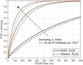
Figure 3: Approximation of Bias Distribution Without Blocking. This figure plots the NLOS bias distribution, derived via Corollary 2 (Solid), against the NLOS bias distribution approximation in Approx. 1 (Dashed). This comparison was made for a test link setup with $d=200m$, and for a Boolean model with reflector widths and orientations distributed as: $f_{W}=\text{unif}(w_{min}=20m,w_{max}=100m,n_{w}=5)$ and $f_{\Theta}=\text{unif}(\theta_{min}=10\degree,\theta_{max}=80\degree,n_{\theta}=8)$.

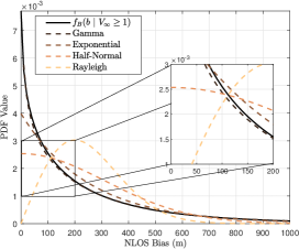
Figure 4: Approximations of Bias Distribution With Blocking. This figure plots the NLOS bias distribution with blocking, derived via Theorem 1, against that of four common exponential family distributions used to model NLOS bias in the localization literature.

III-A2 The Blocking Case

We now turn to the blocking case, which implies we need to condition on the event $\{V_{\infty}\geq 1\}$. Thus, NLOS Bias is given by $B\,|\,\{V_{\infty}\geq 1\}=S_{(1)}\,|\,\{V_{\infty}\geq 1\}-d$, and so it follows from Theorem 1 that $f_{B}(b\,|\,V_{\infty}\geq 1)=f_{S_{(1)}}(b+d\,|\,V_{\infty}\geq 1)$ and $\textbf{Supp}(B\,|\,V_{\infty}\geq 1)=[0,\infty)$. Since we cannot make an obvious connection here between $F_{B}(b\,|\,V_{\infty}\geq 1)$ and an exponential distribution, as was done without blocking, we take a different approach and compare $f_{B}(b\,|\,V_{\infty}\geq 1)$ to various, common distributions of NLOS bias used in the literature.

This comparison is done via the use of the Kullback-Leibler (KL) divergence [28]. Specifically, we examine the KL divergence from $B\,|\,\{V_{\infty}\geq 1\}$ to $X\,|\,\{V_{\infty}\geq 1\}$, i.e.,

$$D(X\,\lvert\rvert\,B)=\int_{0}^{\infty}\!\!\!f_{X}(x\,|\,V_{\infty}\geq 1)\,\ln\Bigg{(}\frac{f_{X}(x\,|\,V_{\infty}\geq 1)}{f_{B}(x\,|\,V_{\infty}\geq 1)}\Bigg{)}\,\text{d}x,$$ (6)

where we choose $X\,|\,\{V_{\infty}\geq 1\}$ to be distributed by one of the four common NLOS bias distributions: gamma, exponential, half-normal, and Rayleigh. First, the parameters of these four comparison distributions were found via ‘moment-matching,’ i.e., the moments of $B\,|\,\{V_{\infty}\geq 1\}$, computed numerically via $f_{B}(b\,|\,V_{\infty}\geq 1)$ using the vales for $d$, $f_{W}$, and $f_{\Theta}$ from Fig. 4, and for $\lambda=10,40,70$ buildings/$km^{2}$ (Table II), were matched to the necessary moments of $X\,|\,\{V_{\infty}\geq 1\}$ to obtain the distributions’ parameter values. Once the parameters of the comparison distributions were found, then the KL divergences from $B\,|\,\{V_{\infty}\geq 1\}$ to $X\,|\,\{V_{\infty}\geq 1\}$ were computed numerically, with the results given in Table II.

Table II reveals that, overall, the gamma distribution provides the best match with our distribution of bias, and, of the single-parameter families, the exponential distribution offers the best approximation. For the $\lambda=40$ case from Table II, we plot the distribution of $B\,|\,\{V_{\infty}\geq 1\}$ and of $X\,|\,\{V_{\infty}\geq 1\}$, for the various moment-matched, comparison distributions, in Fig. 4. From the figure, it is clear that the gamma and exponential distributions offer great approximations, with the gamma distribution approximation being virtually indistinguishable from our analytically derived bias distribution.

TABLE II: Kullback-Leibler Divergence from $B$ to $X$

# of Buildings	$D(X\,\lvert\rvert\,B)$ in nats, where $X$ is distributed by
per $km^{2}$, $\lambda$	$\Gamma(\alpha,\beta)$	$Exp(\beta^{\prime})$	$\frac{1}{2}\mathcal{N}(\sigma)$	$Rayleigh(\sigma^{\prime})$
10	0.0101	0.0238	0.1221	0.4178
40	0.0045	0.0181	0.1104	0.4041
70	0.0022	0.0117	0.0954	0.3793

Motivated by these results, we present a simple, yet accurate, gamma distribution approximation of the NLOS bias for the general blocking case, via moment matching.

Approximation 2 (Distribution of Bias, With Blocking).

Consider $S_{(1)}\,|\,\{V_{\infty}\geq 1\}$ from Theorem 1 for a given test link setup under a Boolean model with set parameters, where its first and second moments, $\mathbb{E}[S_{(1)}\,|\,V_{\infty}\geq 1]$, $\mathbb{E}[S_{(1)}^{2}\,|\,V_{\infty}\geq 1]$, are computed numerically for this particular setup using $f_{S_{(1)}}(s_{(1)}\,|\,V_{\infty}\geq 1)$. Next, the NLOS bias is $B\,|\,\{V_{\infty}\!\geq\!1\}=S_{(1)}\,|\,\{V_{\infty}\!\geq\!1\}-d$, and hence

$$\mathbb{E}[B\,|\,V_{\infty}\!\geq 1]=\mathbb{E}[S_{(1)}|\,V_{\infty}\!\geq 1]-d\,,~{}~{}~{}\mathbb{E}[B^{2}|\,V_{\infty}\!\geq 1]=\mathbb{E}[S_{(1)}^{2}|\,V_{\infty}\!\geq 1]-2d\mathbb{E}[S_{(1)}|\,V_{\infty}\!\geq 1]+d^{2}\!.$$

Then, the gamma distribution approximation of the NLOS bias distribution, $f_{B}$, is given by

$$B\,|\,\{V_{\infty}\geq 1\}\mathbin{\overset{\,\,}{\kern 0.0pt\leavevmode\resizebox{3.33325pt}{3.66875pt}{$\sim$}}}f_{B}(b\,|\,V_{\infty}\geq 1)\approx\tilde{f}_{B}(b\,|\,V_{\infty}\geq 1)=\Gamma(\alpha,\beta),$$

where $\textbf{Supp}(B\,|\,V_{\infty}\geq 1)=[0,\infty)$, which applies to $\tilde{f}_{B}$ as well, and

$$\alpha=\frac{\Big{(}\mathbb{E}[B\,|\,V_{\infty}\geq 1]\Big{)}^{2}}{\mathbb{E}[B^{2}\,|\,V_{\infty}\geq 1]-\Big{(}\mathbb{E}[B\,|\,V_{\infty}\geq 1]\Big{)}^{2}}~{}~{}~{}\text{and}~{}~{}~{}\beta=\frac{\mathbb{E}[B\,|\,V_{\infty}\geq 1]}{\mathbb{E}[B^{2}\,|\,V_{\infty}\geq 1]-\Big{(}\mathbb{E}[B\,|\,V_{\infty}\geq 1]\Big{)}^{2}},$$ (7)

are the shape and rate parameters, respectively.

Proof.

Since $B\,|\,\{V_{\infty}\geq 1\}=S_{(1)}\,|\,\{V_{\infty}\geq 1\}-d$ and from Theorem 1, $\textbf{Supp}(S_{(1)}\,|\,V_{\infty}\geq 1)=[d,\infty)$, then clearly $\textbf{Supp}(B\,|\,V_{\infty}\geq 1)=[0,\infty)$, which we apply to the gamma distribution approximation as well.

Next, we perform moment matching to obtain our gamma distribution approximation of the NLOS bias distribution. Towards this end, we note that in general, if $X\mathbin{\overset{\,\,}{\kern 0.0pt\leavevmode\resizebox{3.33325pt}{3.66875pt}{$\sim$}}}\Gamma(\alpha^{\prime},\beta^{\prime})$, then we may write the parameters, $\alpha^{\prime}$ and $\beta^{\prime}$, in terms of the moments of $X$ as follows:

$$\alpha^{\prime}=\frac{(\mathbb{E}[X])^{2}}{\mathbb{E}[X^{2}]-(\mathbb{E}[X])^{2}},~{}~{}\text{and}~{}~{}~{}\beta^{\prime}=\frac{\mathbb{E}[X]}{\mathbb{E}[X^{2}]-(\mathbb{E}[X])^{2}}.$$ (8)

Since we aim for a gamma distribution approximation, i.e., $\tilde{f}_{B}(b\,|\,V_{\infty}\geq 1)=\Gamma(\alpha,\beta)$, of the NLOS bias distribution, $f_{B}$, we can obtain its parameters by matching the moments of $f_{B}$ with the moments of $\tilde{f}_{B}$. Thus, we write the parameters, $\alpha$ and $\beta$, from $\tilde{f}_{B}(b\,|\,V_{\infty}\geq 1)=\Gamma(\alpha,\beta)$, in terms of the moments of $\tilde{f}_{B}$, as in (8) above. Then, matching moments, we substitute the moments of $f_{B}$ in for those of $\tilde{f}_{B}$ to obtain $\alpha$ and $\beta$ from (7). This completes the approximation. ∎

III-A3 Summary

This section demonstrated that the analytically-derived distribution of NLOS bias, both with and without blocking, are well-approximated by a gamma and exponential distribution, respectively. While a gamma distribution might offer an even better approximation of the bias (than the exponential) in the non-blocking case, as it has two parameters to modify, we note that the exponential approximation is not only sufficient, but it also maintains an elegant simplicity, as evidenced in Approximation 1.

Since the exponential and gamma NLOS bias models presented here are derived via the absolute delay of the first-arriving MPC (the most accurate method for determining NLOS bias to date), then it is fascinating to find that we have arrived at two NLOS bias models that have been assumed in the localization literature, via indirect or heuristic methods, for decades. Thus, this analysis suggests that these two bias models were indeed good assumptions and should perhaps be the standard bias models moving forward, especially for 5G mm-wave.

III-B Numerical Results

Here, we compare our analytically derived NLOS bias distribution against three separate NLOS bias distributions generated via simulation. For our analytically derived bias, $B\,|\,\{V_{\infty}\geq 1\}=S_{(1)}\,|\,\{V_{\infty}\geq 1\}-d$, its distribution is given by $F_{B}(b\,|\,V_{\infty}\geq 1)=F_{S_{(1)}}(b+d\,|\,V_{\infty}\geq 1)$, where the CDF of $S_{(1)}\,|\,\{V_{\infty}\geq 1\}$ is given in Theorem 1. This is labeled as ‘Bias via Theorem 1’ in Figs. 6 and 6. Next, the three comparison bias distributions were generated over $10^{5}$ Boolean model realizations where the path length of the first-arriving NLOS path was recorded in each realization. We now briefly detail how these three distributions were generated.

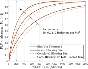
Figure 5: NLOS Bias Distributions: Varying Reflector Density. These results were generated for a test link setup with $d=350m$. The reflector widths were sampled from $f_{W}=\text{unif}(w_{min}=10m,w_{max}=40m,n_{w}=4)$, and orientations from $f_{\Theta}=\text{unif}(\theta_{min}=10\degree,\theta_{max}=80\degree,n_{\theta}=8)$. Note, for each $\lambda$, the first three CDFs listed in the legend overlap each other.

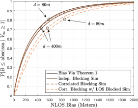
Figure 6: NLOS Bias Distributions: Varying Separation Distance. These results were generated for a reflector density of $\lambda=60$ reflectors per $km^{2}$. The reflector widths and orientations were sampled from the same distributions listed in Fig. 6. Note that for each separation distance, $d$, the first three CDFs listed in the legend overlap, save for the slight deviation in the‘Correlated Blocking Sim’ CDF for $d=80m$.

For the distribution labeled ‘Indep. Blocking Sim’ in Figs. 6 and 6, a Boolean model of reflectors is placed over the test link setup and all reflection paths, without regards to blocking, are noted. Then, each reflection path is checked for blockages by checking whether the incident and reflected paths are blocked using separate Boolean models (Definition 5). Thus, the steps taken to simulate this distribution exactly matches our analytical approach. This simply serves as an extra check on the analysis. From Figs. 6 and 6, we see that, indeed, this does match our analytical distribution (it is not visible, as it exactly overlaps with the analytical bias CDF).

For the distribution labeled ‘Correlated Blocking Sim’ in Figs. 6 and 6, a Boolean model of reflectors is placed as above. However, now each reflection path is checked for blockages using this same Boolean model. This represents true, correlated blocking on reflection paths. In almost all cases plotted, this virtually overlaps the previous two distributions, indicating that the independent blocking assumption accurately captures correlated blocking on reflection paths.

Finally, we conduct a simulation similar to ‘Correlated Blocking Sim’ above, but with the extra restriction that only Boolean model realizations where the LOS path is blocked by at least one reflector are considered. This departs from the Boolean model assumption, due to the forced conditioning, and also represents an extreme case of correlated blocking. The bias distribution generated in this case is labeled ‘Corr. Blocking w/ LOS Blocked Sim’ in Figs. 6 and 6.

For the first result in Fig. 6, these four distributions above were plotted for different reflector densities. As the reflector density increases, the bias distributions shift to the left – a trend that matches intuition. Additionally, the close match with the ‘Corr. Blocking w/ LOS Blocked Sim’ case indicates that the analytical bias model, which assumes independent blocking, can reasonably capture the effect of forced blockages. We explore this case further below, along with it’s match with the analytical bias and possible corner-cases.

In Fig. 6, the density of reflectors, as well as their size and orientation distributions, remained constant and the only parameter that changed was the base station-mobile separation distance, $\!d$. We can see that as the base station and mobile begin to close in on each other, the ‘Corr. Blocking w/ LOS Blocked Sim’ CDF begins to deviate slightly from the other three CDFs. This occurs due to the conditioning in the ‘Corr. Blocking w/ LOS Blocked Sim’ case, where at least one reflector is forced between the base station and mobile; blocking the LOS path. As $d$ decreases, the buildings appear larger in relation to this base station-mobile separation distance, and thus, forcing at least one large building in between the two introduces significant correlated blocking. For example, when $d=80m$, if the largest reflector, $w=40m$, is placed appropriately, it can take up to $\sim\!\!70\%$ of the separation distance, thus having the potential to block many reflection paths at once. For the reader accustomed to examining positioning error distributions, bias error, relatively speaking, is significantly larger, often on the order of hundreds of meters to a few kilometers, [29], [13]. Thus, despite the amount of correlated blocking introduced in the $d=80m$ case, the deviation of the ‘Corr. Blocking w/ LOS Blocked Sim’ CDF from the other three CDFs is surprisingly small. Consequently, the independent blocking assumption holds reasonably well in these cases of significant correlated blocking. That being said, placing the base station and mobile at the extreme ends of a large building, so that the building covers $\sim\!\!100\%$ of the separation distance, will almost certainly cause the independent blocking assumption to break down and the accuracy of the analytical bias distribution to degrade. As with any analytical model, it is always important to be aware of such model limitations and ‘corner cases’.

III-C Discussion

To the authors’ knowledge, no outdoor measurement campaigns characterizing NLOS bias currently exist. This observation was noted in 1996 [30], and was echoed again in 2007 [14]:

At the present time, very little is known about the statistics of the NLOS variables [bias] in realistic propagation environments, and there are no established models.

and we believe this lack of measurement data characterizing NLOS bias still exists to this day.

Appropriately characterizing the NLOS bias outdoors requires measuring the absolute delay of the first-arriving MPC under NLOS conditions. This is difficult for a number of reasons, the first of which is the need for highly-accurate, nanosecond-level (or less) synchronization between the Tx and Rx. Not many non-tethered channel sounders exist that offer enough bandwidth, along with the accurate synchronization necessary, to perform the absolute TOF measurements needed [31]. Additionally, the measurements themselves are tedious due to the need for Rubidium clocks at the Tx and Rx which require a “synchronization training period” of an hour or more and which can fall out of synchronization just as quickly [31]. Furthermore, the Tx and Rx would require accurate GPS positioning in order to extract the bias, which can be hard to obtain depending on the measurement environment, e.g., urban canyons. Finally, these measurements would need to occur, for a given Tx-Rx separation distance, over many realizations of the surrounding environment in order to generate statistics of the bias. Thus, deriving accurate analytical bias models, such as those presented here, is necessary due to these difficulties in empirically characterizing the NLOS bias.

Given this lack of data with which to compare our bias distributions against, it is reasonable to ask: “What can be gleaned about NLOS bias from other (semi-related) measurement-based models that already exist in the literature?” To answer this, we attempt to glean insight into the nature of NLOS bias by examining a mm-wave channel model of excess multipath delays derived from outdoor LOS measurements. From the model in [32], excess delays of MPCs from LOS PDPs are sampled from an exponential distribution, which was derived via a fit to measurement data. Supposing these multipath delays are independent, then the excess delay of the first-arriving multipath component is also exponentially distributed. Since the measurements are LOS, then to obtain the absolute delay, one can simply add on the LOS TOF, which is a simple shift of the exponential distribution. Finally, if we assume that there is a blockage that 1) removes the LOS component, and 2) is not significantly correlated with the first-arriving reflection path, then there is reason to believe that this shifted exponential distribution can reasonably represent the absolute delay of the first-arriving MPC in a NLOS scenario. (Similar reasoning is also given in [21].) This evidence suggests that the distribution for the path length (i.e., absolute delay) of the first-arriving MPC presented here is at least “in-line” with what one would expect in reality.

We conclude this section by noting that Theorem 1, i.e., the distribution of the first-arriving MPC, can also be used in channel simulators [33] to provide a distribution from which to sample an absolute timing reference for excess delay PDPs in NLOS scenarios.

IV The Angle-of-Arrival of the First-Arriving Reflection

This section derives the AOA distribution of the first-arriving reflected path, with blocking. We begin with some important AOAs which correspond to the boundary PRPs from Lemma 2.

Definition 8 (The $s$-Meter AOAs for $\mathcal{R}_{w,\theta,\mathbf{c}}$).

Recall from Lemma 2 that there are precisely four PRPs that reflector $\mathcal{R}_{w,\theta,\mathbf{c}}$ can intersect to produce a reflection of exactly $s$ meters, where $d<s<\infty$. These PRPs are labeled, $\mathbf{h}_{\text{I},\theta}(s)$, $\mathbf{h}_{\text{II},\theta}(s)$, $\mathbf{h}_{\text{III},\theta}(s)$, $\mathbf{h}_{\text{IV},\theta}(s)$. If $\partial\mathcal{R}_{w,\theta,\mathbf{c}}$ were to intersect $\mathbf{h}_{q,\theta}(s)$ ($q\in\mathcal{Q}$) to produce a reflection, then we label the AOA at $\mathbf{m}$ of the reflected path, $\mathcal{L}_{[\mathbf{h}_{q,\theta}(s),\mathbf{m}]}$, by $\psi_{q,\theta}(s)$, which is measured in radians c.c.w. w.r.t. the $+x$-axis. We call these four AOAs the $s$-meter AOAs for $\mathcal{R}_{w,\theta,\mathbf{c}}$. The $Q_{\text{I}}$ $s_{1}$-meter AOA for $\mathcal{R}_{w,\theta_{j},\mathbf{c}}$ is depicted in Fig. 2.

Observe, for example, the $Q_{\text{I}}$ $s_{1}$-meter AOA for $\mathcal{R}_{w,\theta_{j},\mathbf{c}}$, i.e., $\psi_{\text{I},\theta_{j}}(s_{1})$, in Fig. 2. Note that as $s_{1}$ increases, $\mathbf{h}_{\text{I},\theta_{j}}(s_{1})$ tracks along the reflection hyperbola, $\mathcal{H}_{\theta_{j}}$, as the $s_{1}$-ellipse boundary, $\partial\mathcal{P}_{s_{1}}$, expands out. Consequently, the corresponding AOA, $\psi_{\text{I},\theta_{j}}(s_{1})$, changes as well. Hence, the $s$-meter AOAs for $\mathcal{R}_{w,\theta,\mathbf{c}}$ are functions of $s$ (parameterized by $\theta$). Their behavior as functions of $s$ is of particular importance in subsequent derivations and so we present the following lemma.

Lemma 5 (The $s$-meter AOA Functions for $\mathcal{R}_{w,\theta,\mathbf{c}}$).

The $s$-meter AOA functions for $\mathcal{R}_{w,\theta,\mathbf{c}}$, i.e., $\alpha=\psi_{q,\theta}(s)$, for $q\in\mathcal{Q}$, are given in Table III, along with their derivatives and inverses.

TABLE III: The $s$-Meter AOA Functions for $\mathcal{R}_{w,\theta,\mathbf{c}}$, i.e., $\alpha=\psi_{q,\theta}(s)$, Their Derivatives, and Respective Inverses

$\psi_{\text{I},\theta}(s)=\cos^{-1}\!\!\Big{(}\!-\!\frac{d\sin\theta}{s}\Big{)}\!+\!\theta\!-\!\frac{\pi}{2}$,	$d\leq s<\infty$	$\psi_{\text{I},\theta}^{\prime}(s)=-\frac{d\sin\theta}{s\sqrt{s^{2}-d^{2}\sin^{2}\theta}}$,	$d\leq s<\infty$
$\psi_{\text{I},\theta}^{-1}(\alpha)=\frac{d\sin\theta}{\sin\big{(}\alpha-\theta\big{)}}$,	$\theta<\alpha\leq 2\theta$	$\big{(}\psi_{\text{I},\theta}^{-1}\big{)}^{\prime}(\alpha)=-\psi_{\text{I},\theta}^{-1}(\alpha)\cot\big{(}\alpha\!-\theta\big{)}$,	$\theta<\alpha\leq 2\theta$
$\psi_{\text{II},\theta}(s)=\cos^{-1}\!\!\Big{(}\!-\!\frac{d\cos\theta}{s}\Big{)}\!+\!\theta$,	$d\leq s<\infty$	$\psi_{\text{II},\theta}^{\prime}(s)=-\frac{d\cos\theta}{s\sqrt{s^{2}-d^{2}\cos^{2}\theta}}$,	$d\leq s<\infty$
$\psi_{\text{II},\theta}^{-1}(\alpha)=\frac{-d\cos\theta}{\cos\big{(}\alpha-\theta\big{)}}$,	$\frac{\pi}{2}+\theta<\alpha\leq\pi$	$\big{(}\psi_{\text{II},\theta}^{-1}\big{)}^{\prime}(\alpha)=\psi_{\text{II},\theta}^{-1}(\alpha)\tan\big{(}\alpha\!-\theta\big{)}$,	$\frac{\pi}{2}+\theta<\alpha\leq\pi$
$\psi_{\text{III},\theta}(s)=\cos^{-1}\!\!\Big{(}\frac{d\sin\theta}{s}\Big{)}\!+\!\theta\!+\!\frac{\pi}{2}$,	$d\leq s<\infty$	$\psi_{\text{III},\theta}^{\prime}(s)=\frac{d\sin\theta}{s\sqrt{s^{2}-d^{2}\sin^{2}\theta}}$,	$d\leq s<\infty$
$\psi_{\text{III},\theta}^{-1}(\alpha)=\frac{d\sin\theta}{\sin\big{(}\alpha-\theta\big{)}}$,	$\pi\leq\alpha<\pi+\theta$	$\big{(}\psi_{\text{III},\theta}^{-1}\big{)}^{\prime}(\alpha)=-\psi_{\text{III},\theta}^{-1}(\alpha)\cot\big{(}\alpha\!-\theta\big{)}$,	$\pi\leq\alpha<\pi+\theta$
$\psi_{\text{IV},\theta}(s)=\cos^{-1}\!\!\Big{(}\frac{d\cos\theta}{s}\Big{)}\!+\!\theta\!+\!\pi$,	$d\leq s<\infty$	$\psi_{\text{IV},\theta}^{\prime}(s)=\frac{d\cos\theta}{s\sqrt{s^{2}-d^{2}\cos^{2}\theta}}$,	$d\leq s<\infty$
$\psi_{\text{IV},\theta}^{-1}(\alpha)=\frac{-d\cos\theta}{\cos\big{(}\alpha-\theta\big{)}}$,	$\pi\!+\!2\theta\!\leq\alpha\!<\!\frac{3\pi}{2}\!+\!\theta$	$\big{(}\psi_{\text{IV},\theta}^{-1}\big{)}^{\prime}(\alpha)=\psi_{\text{IV},\theta}^{-1}(\alpha)\tan\big{(}\alpha\!-\theta\big{)}$,	$\pi\!+\!2\theta\!\leq\alpha\!<\!\frac{3\pi}{2}\!+\!\theta$

Proof.

We present only the derivation of the $Q_{\text{I}}$ $s$-meter AOA function for $\mathcal{R}_{w,\theta,\mathbf{c}}$, i.e. $\psi_{\text{I},\theta}(s)$, as the other quadrant $s$-meter AOA functions follow similarly. We begin by recalling from Definition 8 that $\psi_{\text{I},\theta}(s)$ is the angle of the slope of the reflection path $\mathcal{L}_{[\mathbf{h}_{\text{I},\theta}(s),\mathbf{m}]}$. Thus, letting $\alpha=\psi_{\text{I},\theta}(s)$, we have the relationship: $\tan(\alpha)=\frac{-[\mathbf{h}_{\text{I},\theta}(s)]_{2}}{\frac{d}{2}-[\mathbf{h}_{\text{I},\theta}(s)]_{1}}$, which leads to the following:

$$\alpha=\psi_{\text{I},\theta}(s)=\begin{cases}\tan^{-1}\!\left[\frac{d^{2}-s^{2}}{d\sqrt{s^{2}\csc^{2}\theta-d^{2}}-s^{2}\cot\theta}\right],&\!\frac{d^{2}-s^{2}}{d\sqrt{s^{2}\csc^{2}\theta-d^{2}}-s^{2}\cot\theta}\geq 0\\ \tan^{-1}\!\left[\frac{d^{2}-s^{2}}{d\sqrt{s^{2}\csc^{2}\theta-d^{2}}-s^{2}\cot\theta}\right]+\pi,&\!\frac{d^{2}-s^{2}}{d\sqrt{s^{2}\csc^{2}\theta-d^{2}}-s^{2}\cot\theta}<0\\[-0.86108pt] \end{cases},~{}~{}\text{for}~{}~{}d<s<\infty.\vspace{-16pt}$$ (9)

This follows from simplifying the r.h.s. of the above relationship using Lemma 2, taking $\tan^{-1}\!(\cdot)$ of both sides, and noting that for $-\infty\leq x<0$, $\textbf{Range}\big{(}\!\tan^{-1}(x)\big{)}=[\pi/2,0)$, and so $\pi$ must be added when the slope of the reflection path is negative. Finally, taking $\cos^{-1}\!\big{(}\!\cos(\cdot)\big{)}$ of the r.h.s. in (9) and simplifying yields the expression for $\psi_{\text{I},\theta}(s)$ in Table III for $d<s<\infty$. ∎

Definition 9 (AOA of the $1^{\text{st}}$-Arriving Reflection).

Let $A_{(1)}$ be the RV representing the AOA, in radians, of the first-arriving reflection, measured c.c.w. w.r.t. the $+x$-axis. Note, $0<A_{(1)}<2\pi$.

Remark.

Although the distribution of $S_{(1)}$ was derived assuming the LOS path was blocked, Assumption 3 asserts that $f_{S_{(1)}}(s_{(1)}\,|\,V_{\infty}\geq 1)$ does not change when blocking on the LOS path is ignored. Consequently, moving forward, we simply assume $f_{S_{(1)}}(s_{(1)}\,|\,V_{\infty}\geq 1)$ was derived irrespective of what happens on the LOS path. Since we also seek to derive the distribution of $A_{(1)}$ irrespective of what happens on the LOS path, then the distributions of $S_{(1)}$ and $A_{(1)}$ will both characterize the first-arriving reflection under the same conditions. This implies that $S_{(1)}$ and $A_{(1)}$ each describe different properties of the same first-arriving reflection path; hence, $A_{(1)}$ is subject to the same existence issues as $S_{(1)}$, and so must be conditioned on $\{V_{\infty}\geq 1\}$ as well.

Lemma 6 ($A_{(1)}$ Conditional Distribution Given $S_{(1)}$).

Consider the test link setup and Boolean model. Then, the conditional PDF of $A_{(1)}$ given a first-arriving reflection of distance $S_{(1)}$ is: $f_{A_{(1)}}(\alpha_{(1)}\,|\,S_{(1)},V_{\infty}\geq 1)=\frac{1}{\sum_{j^{\prime}=1}^{n_{\theta}}\sum_{q^{\prime}\in\mathcal{Q}}\omega_{q^{\prime},\theta_{j^{\prime}}}(s_{(1)})}\sum_{j=1}^{n_{\theta}}\sum_{q\in\mathcal{Q}}\omega_{q,\theta_{j}}(s_{(1)})\,\delta\Big{(}\alpha_{(1)}-\psi_{q,\theta_{j}}(s_{(1)})\Big{)}$, where $\omega_{\text{\emph{I}},\theta_{j}}(s_{(1)})$, $\omega_{\text{\emph{II}},\theta_{j}}(s_{(1)})$, $\omega_{\text{\emph{III}},\theta_{j}}(s_{(1)})$, and $\omega_{\text{\emph{IV}},\theta_{j}}(s_{(1)})$, are given, respectively, by:

$$\rho\big{(}\mathbf{h}_{\text{\emph{I}},\theta_{j}}(s_{(1)})\big{)}\textstyle\frac{s_{(1)}\big{(}\psi^{-1}_{\text{\emph{I}},\theta_{j}}\big{)}^{\prime}\big{(}\psi_{\text{\emph{I}},\theta_{j}}(s_{(1)})\big{)}}{2\sqrt{s_{(1)}^{2}-d^{2}\sin^{2}\!\theta_{j}}}\psi_{\text{\emph{I}},\theta_{j}}^{\prime}(s_{(1)}),~{}~{}~{}~{}~{}~{}~{}~{}\rho\big{(}\mathbf{h}_{\text{\emph{II}},\theta_{j}}(s_{(1)})\big{)}\textstyle\frac{s_{(1)}\big{(}\psi^{-1}_{\text{\emph{II}},\theta_{j}}\big{)}^{\prime}\big{(}\psi_{\text{\emph{II}},\theta_{j}}(s_{(1)})\big{)}}{2\sqrt{s_{(1)}^{2}-d^{2}\cos^{2}\!\theta_{j}}}\psi_{\text{\emph{II}},\theta_{j}}^{\prime}(s_{(1)})$$

$$\rho\big{(}\mathbf{h}_{\text{\emph{III}},\theta_{j}}(s_{(1)})\big{)}\textstyle\frac{s_{(1)}\big{(}\psi^{-1}_{\text{\emph{III}},\theta_{j}}\big{)}^{\prime}\big{(}\psi_{\text{\emph{III}},\theta_{j}}(s_{(1)})\big{)}}{2\sqrt{s_{(1)}^{2}-d^{2}\sin^{2}\!\theta_{j}}}\psi_{\text{\emph{III}},\theta_{j}}^{\prime}(s_{(1)}),~{}~{}~{}\rho\big{(}\mathbf{h}_{\text{\emph{IV}},\theta_{j}}(s_{(1)})\big{)}\textstyle\frac{s_{(1)}\big{(}\psi^{-1}_{\text{\emph{IV}},\theta_{j}}\big{)}^{\prime}\big{(}\psi_{\text{\emph{IV}},\theta_{j}}(s_{(1)})\big{)}}{2\sqrt{s_{(1)}^{2}-d^{2}\cos^{2}\!\theta_{j}}}\psi_{\text{\emph{IV}},\theta_{j}}^{\prime}(s_{(1)}),$$

$\mathbf{h}_{q,\theta_{j}}$, $\rho(\cdot)$, and $\psi_{q,\theta_{j}}$ from Lemmas 2, 3, and 5, respectively, and $\textbf{\emph{Supp}}(A_{(1)}\,|\,S_{(1)},V_{\infty}\!\geq\!1)\!=\!\big{\{}\psi_{q,\theta_{j}}(s_{(1)})\big{\}}$ for $q\!\in\!\mathcal{Q}$, $j\!\in\!\{1,\dots,n_{\theta}\}$.

Proof.

Let $S_{(1)}=s_{(1)}$ and consider all of the boundary PRPs, $\mathbf{h}_{q,\theta_{j}}(s_{(1)})$ ($q\in\mathcal{Q}$, $j\in\{1,\dots,n_{\theta}\}$) that reflectors of $\mathcal{B}$ can intersect to produce the first-arriving reflection path of distance $s_{(1)}$. (Letting $s_{1}=s_{(1)}$, Fig. 2 gives an example depiction of four of these PRPs, i.e., those associated with a reflector of orientation $\theta_{j}$. The PRPs for the reflectors of other orientations would be placed along $\partial\mathcal{P}_{s_{(1)}}$ as well, if depicted.) Recall from Definition 8, that associated with each of these PRPs is an AOA for the reflected path, $\psi_{q,\theta_{j}}(s_{(1)})$. Since there are ‘$4n_{\theta}$’ potential AOAs, we must determine the probability $A_{(1)}$ equals any one of them. Thus, we seek a conditional distribution of the form stated in the lemma, where each possible AOA, $\psi_{q,\theta}(s_{(1)})$, has associated with it a weighting factor, $\omega_{q,\theta_{j}}(s_{(1)})$, where $P[A_{(1)}=\psi_{q,\theta}(s_{(1)})\,|\,S_{(1)},V_{\infty}]=\frac{\omega_{q,\theta_{j}}(s_{(1)})}{\sum_{j^{\prime}=1}^{n_{\theta}}\sum_{q^{\prime}\in\mathcal{Q}}\omega_{q^{\prime},\theta_{j^{\prime}}}(s_{(1)})}$.

Correctly determining these weighting factors requires conditioning on $S_{(1)}$ being within an infinitesimal sliver: $f_{A_{(1)}}(\alpha_{(1)}\,|\,S_{(1)},V_{\infty}\geq 1)=\lim_{\Delta s_{(1)}\to 0}f_{A_{(1)}}(\alpha_{(1)}\,|\,s_{(1)}\leq S_{(1)}\leq s_{(1)}+\Delta s_{(1)},V_{\infty}\geq 1)$. In so doing, by ignoring zero probability events in this conditioning, we can choose $\Delta s_{(1)}$ s.t. one and only one reflector produces a reflection with distance in $[s_{(1)},s_{(1)}+\Delta s_{(1)}]$, which is that producing the first-arriving reflection. This implies we have conditioned on one and only one reflector having a VRP in ‘$\mathcal{P}_{s_{(1)}+\Delta s_{(1)}}/(\mathcal{P}_{s_{(1)}}/\partial\mathcal{P}_{s_{(1)}})$.’ Now, there are ‘$4n_{w}n_{\theta}$’ mutually exclusive ways, or “sub-events,” in which this reflector can produce a VRP in ‘$\mathcal{P}_{s_{(1)}+\Delta s_{(1)}}/(\mathcal{P}_{s_{(1)}}/\partial\mathcal{P}_{s_{(1)}})$,’ with the typical sub-event being the center point of edge $\mathcal{E}_{q}$ of $\mathcal{R}_{w_{i},\theta_{j},\mathbf{c}}$ (for $q\in\mathcal{Q},i\in\{1,\dots,n_{w}\},j\in\{1,\dots,n_{\theta}\}$) falling in $\Omega_{q}=\mathcal{E}_{q}\oplus\big{(}\mathcal{H}_{\theta_{j}}\cap Q_{q}\cap\mathcal{P}_{s_{(1)}+\Delta s_{(1)}}/(\mathcal{P}_{s_{(1)}}/\partial\mathcal{P}_{s_{(1)}})\big{)}$ (see proof of Lemma 4 for $\mathcal{E}_{q}$ definition). Letting $s_{1}=s_{(1)}$ and $s_{2}=s_{(1)}+\Delta s_{(1)}$, Fig. 2 depicts four of these sub-events for $\mathcal{R}_{w_{i},\theta_{j},\mathbf{c}}$. Examining Fig. 2, we note that as $\Delta s_{(1)}\to 0$, the $\mathcal{E}_{\text{I}}$ edge center point of $\mathcal{R}_{w_{i},\theta_{j},\mathbf{c}}$ falling in $\Omega_{\text{I}}$ implies that the RP for the first-arriving reflection is at $\mathbf{h}_{\text{I},\theta_{j}}(s_{(1)})\implies A_{(1)}=\psi_{\text{I},\theta_{j}}(s_{(1)})$. Thus, we now have a way for determining whether $A_{(1)}$ equals any of the ‘$4n_{\theta}$’ potential AOAs, since this occurs if the reflector producing the first-arriving reflection falls in one of the corresponding sub-events, i.e., $\Omega_{\text{I}},\Omega_{\text{II}},\Omega_{\text{III}},\Omega_{\text{IV}}$ for $\mathcal{R}_{w_{i},\theta_{j},\mathbf{c}}$. This yields $f_{A_{(1)}}(\alpha_{(1)}\,|\,s_{(1)}\leq S_{(1)}\leq s_{(1)}+\Delta s_{(1)},V_{\infty}\geq 1)=$

$$\frac{\frac{1}{n_{w}}\frac{1}{n_{\theta}}\!\!\sum\limits_{j=1}^{n_{\theta}}\sum\limits_{q\in\mathcal{Q}}\sum\limits_{i=1}^{n_{w}}\!w_{i}\Gamma_{q,\theta_{j}}(s_{(1)})\,\delta\Big{(}\alpha_{(1)}-\psi_{q,\theta_{j}}(s_{(1)})\!\Big{)}}{\frac{1}{n_{w}}\frac{1}{n_{\theta}}\!\sum_{j^{\prime}=1}^{n_{\theta}}\sum_{q^{\prime}\in\mathcal{Q}}\sum_{i^{\prime}=1}^{n_{w}}\!w_{i^{\prime}}\Gamma_{q^{\prime},\theta_{j^{\prime}}}(s_{(1)})}=\frac{\sum\limits_{j=1}^{n_{\theta}}\sum\limits_{q\in\mathcal{Q}}\!\!\Gamma_{q,\theta_{j}}(s_{(1)})\,\delta\Big{(}\alpha_{(1)}-\psi_{q,\theta_{j}}(s_{(1)})\!\Big{)}}{\sum_{j^{\prime}=1}^{n_{\theta}}\sum_{q^{\prime}\in\mathcal{Q}}\Gamma_{q^{\prime},\theta_{j^{\prime}}}(s_{(1)})},$$ (10)

where $\Gamma_{\text{I},\theta_{j}}(s_{(1)})$, $\Gamma_{\text{II},\theta_{j}}(s_{(1)})$, $\Gamma_{\text{III},\theta_{j}}(s_{(1)})$, and $\Gamma_{\text{IV},\theta_{j}}(s_{(1)})$ are given, respectively, by

$$\int\limits_{[\mathbf{R}_{\theta_{j}}\mathbf{h}_{\text{I},\theta_{j}}(s_{(1)})]_{1}}^{[\mathbf{R}_{\theta_{j}}\mathbf{h}_{\text{I},\theta_{j}}(s_{(1)}+\Delta s_{(1)})]_{1}}\!\!\!\!\!\!\!\!\!\!\!\!\!\!\!\!\!\!\!\!\!\!\rho\Big{(}\mathbf{R}^{-1}_{\theta_{j}}\mathbf{g}^{*}_{\text{I}}(x_{\theta_{j}}\!)\!\Big{)}\text{d}x_{\theta_{j}},~{}\!\!\!\!\!\!\!\!\!\!\!\!\!\!\!\!\!\!\!\!\int\limits_{[\mathbf{R}_{\theta_{j}}\mathbf{h}_{\text{II},\theta_{j}}(s_{(1)})]_{2}}^{[\mathbf{R}_{\theta_{j}}\mathbf{h}_{\text{II},\theta_{j}}(s_{(1)}+\Delta s_{(1)})]_{2}}\!\!\!\!\!\!\!\!\!\!\!\!\!\!\!\!\!\!\!\!\!\!\rho\Big{(}\mathbf{R}^{-1}_{\theta_{j}}\mathbf{g}^{*}_{\text{II}}(y_{\theta_{j}}\!)\!\Big{)}\text{d}y_{\theta_{j}},~{}\!\!\!\!\!\!\!\!\!\!\!\!\!\!\!\!\!\!\!\!\!\int\limits_{[\mathbf{R}_{\theta_{j}}\mathbf{h}_{\text{III},\theta_{j}}(s_{(1)}+\Delta s_{(1)})]_{1}}^{[\mathbf{R}_{\theta_{j}}\mathbf{h}_{\text{III},\theta_{j}}(s_{(1)})]_{1}}\!\!\!\!\!\!\!\!\!\!\!\!\!\!\!\!\!\!\!\!\!\!\!\rho\Big{(}\mathbf{R}^{-1}_{\theta_{j}}\mathbf{g}^{*}_{\text{III}}(x_{\theta_{j}}\!)\!\Big{)}\text{d}x_{\theta_{j}},~{}\!\!\!\!\!\!\!\!\!\!\!\!\!\!\!\!\!\!\!\!\!\!\int\limits_{[\mathbf{R}_{\theta_{j}}\mathbf{h}_{\text{IV},\theta_{j}}(s_{(1)}+\Delta s_{(1)})]_{2}}^{[\mathbf{R}_{\theta_{j}}\mathbf{h}_{\text{IV},\theta_{j}}(s_{(1)})]_{2}}\!\!\!\!\!\!\!\!\!\!\!\!\!\!\!\!\!\!\!\!\!\!\!\rho\Big{(}\mathbf{R}^{-1}_{\theta_{j}}\mathbf{g}^{*}_{\text{IV}}(y_{\theta_{j}}\!)\!\Big{)}\text{d}y_{\theta_{j}}.$$

Here, each sub-event from above is weighted by ‘$\frac{1}{n_{w}}\frac{1}{n_{\theta}}w_{i}\Gamma_{\!q,\theta_{j}}\!(\!s_{(1)}\!)$,’ where ‘$\frac{1}{n_{w}}\frac{1}{n_{\theta}}$’ is the probability $\mathcal{R}_{w_{i},\theta_{j},\mathbf{c}}$ is selected and ‘$w_{i}\Gamma_{\!q,\theta_{j}}\!(\!s_{(1)}\!)$’ is the probability its $\mathcal{E}_{q}$ edge center point falls in $\Omega_{q}$ to create a visible reflection, as opposed to the other $\Omega_{q}$ regions (see Fig. 2). Note that ‘$w_{i}\Gamma_{\!\text{I},\theta_{j}}\!(\!s_{(1)}\!)$’ was derived in the same manner as in (5), and simply computes the area of $\Omega_{\text{I}}$, where each $\mathbf{x}\in\Omega_{\text{I}}$ is weighted by the probability its corresponding edge produces a visible reflection. We refer the reader to the proof of Lemma 4 for further details. The other ‘$w_{i}\Gamma_{\!q,\theta_{j}}(\!s_{(1)}\!)$’ are derived similarly.

Next, it’s easiest to work with these integrals when they are evaluated w.r.t. a common AOA variable. Thus, consider the transformations: for $\Gamma_{\text{I},\theta_{j}}(s_{(1)})$, let $x_{\theta_{j}}=\big{[}\mathbf{R}_{\theta_{j}}\mathbf{h}_{\text{I},\theta_{j}}\big{(}\psi_{\text{I},\theta_{j}}^{-1}(\alpha)\big{)}\big{]}_{1}$, for $\Gamma_{\text{II},\theta_{j}}(s_{(1)})$, let $y_{\theta_{j}}=\big{[}\mathbf{R}_{\theta_{j}}\mathbf{h}_{\text{II},\theta_{j}}\big{(}\psi_{\text{II},\theta_{j}}^{-1}(\alpha)\big{)}\big{]}_{2}$, for $\Gamma_{\text{III},\theta_{j}}(s_{(1)})$, let $x_{\theta_{j}}=\big{[}\mathbf{R}_{\theta_{j}}\mathbf{h}_{\text{III},\theta_{j}}\big{(}\psi_{\text{III},\theta_{j}}^{-1}(\alpha)\big{)}\big{]}_{1}$, and for $\Gamma_{\text{IV},\theta_{j}}(s_{(1)})$, let $y_{\theta_{j}}=\big{[}\mathbf{R}_{\theta_{j}}\mathbf{h}_{\text{IV},\theta_{j}}\big{(}\psi_{\text{IV},\theta_{j}}^{-1}(\alpha)\big{)}\big{]}_{2}$. For $\Gamma_{\text{I},\theta_{j}}(s_{(1)})$, this transformation implies $\text{d}x_{\theta_{j}}=\big{[}\mathbf{R}_{\theta_{j}}\frac{\text{d}}{\text{d}\alpha}\mathbf{h}_{\text{I},\theta_{j}}\big{(}\psi_{\text{I},\theta_{j}}^{-1}(\alpha)\big{)}\big{]}_{1}\text{d}\alpha$, which yields

$$\Gamma_{\text{I},\theta_{j}}(s_{(1)})\stackrel{{\scriptstyle(a)}}{{=}}\int_{\psi_{\text{I},\theta_{j}}(s_{(1)})}^{\psi_{\text{I},\theta_{j}}(s_{(1)}+\Delta s_{(1)})}\!\!\!\!\!\!\!\!\!\!\!\!\!\!\!\rho\Big{(}\mathbf{h}_{\text{I},\theta_{j}}\big{(}\psi_{\text{I},\theta_{j}}^{-1}(\alpha)\big{)}\!\Big{)}\Big{[}\mathbf{R}_{\theta_{j}}\textstyle\frac{\text{d}}{\text{d}\alpha}\mathbf{h}_{\text{I},\theta_{j}}\big{(}\psi_{\text{I},\theta_{j}}^{-1}(\alpha)\big{)}\Big{]}_{\!1}\text{d}\alpha$$ (11)

$$\!\!\stackrel{{\scriptstyle(b)}}{{=}}\!\!\rho\Big{(}\mathbf{h}_{\text{I},\theta_{j}}\!\big{(}s_{(1)}\big{)}\!\Big{)}\!\Big{[}\mathbf{R}_{\theta_{j}}\textstyle\frac{\text{d}}{\text{d}\alpha}\!\big{[}\mathbf{h}_{\text{I},\theta_{j}}\!\big{(}\psi_{\text{I},\theta_{j}}^{-1}\!(\alpha)\big{)}\!\big{]}_{\alpha=\psi_{\text{I},\theta_{j}}(s_{(1)})}\!\Big{]}_{\!1}\!\Big{(}\psi_{\text{I},\theta_{j}}\!(s_{(1)}\!+\!\Delta s_{(1)})-\psi_{\text{I},\theta_{j}}\!(s_{(1)})\!\Big{)}\!\stackrel{{\scriptstyle(c)}}{{=}}\!\omega_{\text{I},\theta_{j}}\!(s_{(1)})\Delta s_{(1)},$$

where (a) applies the transformation, (b) is the evaluation of the integral as “base-times-height” when driving $\Delta s_{(1)}\to 0$, and (c) follows by simplifying $[\cdot]_{1}$ and by the definition of the derivative of $\psi_{\text{I},\theta_{j}}(s_{(1)})$ when driving $\Delta s_{(1)}\to 0$ ($\omega_{\text{I},\theta_{j}}(s_{(1)})$ is given in the lemma statement). Following the same procedure, we obtain: $\Gamma_{\text{II},\theta_{j}}(s_{(1)})\!=\!\omega_{\text{II},\theta_{j}}(s_{(1)})\Delta s_{(1)}$, $\Gamma_{\text{III},\theta_{j}}(s_{(1)})\!=\!\omega_{\text{III},\theta_{j}}(s_{(1)})\Delta s_{(1)}$, and $\Gamma_{\text{IV},\theta_{j}}(s_{(1)})=\omega_{\text{IV},\theta_{j}}(s_{(1)})\Delta s_{(1)}$. Finally, substituting these into (10), the $\Delta s_{(1)}$’s cancel, and taking $\lim_{\Delta s_{(1)}\to 0}$ ensures our approximations (b) and (c) in (11) are, in fact, equalities in the limit. ∎

Theorem 2 ($A_{(1)}$ Marginal Distribution).

Consider the test link setup and Boolean model. Then, the marginal PDF of $A_{(1)}$ is given by:

$$f_{\!A_{(1)}}(\alpha_{(1)}\,|\,V_{\infty}\!\geq\!1)=\!\sum\limits_{j=1}^{n_{\theta}}\sum\limits_{q\in\mathcal{Q}}\left[\!\frac{\Big{(}\psi_{q,\theta_{j}}^{-1}\Big{)}^{\prime}\!\!(\alpha_{(1)})\,\omega_{q,\theta_{j}}\Big{(}\psi_{q,\theta_{j}}^{-1}(\alpha_{(1)})\!\Big{)}f_{S_{(1)}}\Big{(}\psi_{q,\theta_{j}}^{-1}(\alpha_{(1)})\,\Big{|}\,V_{\infty}\!\geq\!1\Big{)}}{\sum_{j^{\prime}=1}^{n_{\theta}}\sum_{q^{\prime}\in\mathcal{Q}}\omega_{q^{\prime},\theta_{j^{\prime}}}\Big{(}\psi_{q,\theta_{j}}^{-1}(\alpha_{(1)})\Big{)}}\beta_{q,\theta_{j}}(\alpha_{(1)})\right],$$

where $\beta_{\text{\emph{I}},\theta_{j}}(\alpha_{(1)})=-\mathbbm{1}[\theta_{j}<\alpha_{(1)}\leq 2\theta_{j}]$, $\beta_{\text{\emph{II}},\theta_{j}}(\alpha_{(1)})=-\mathbbm{1}[\frac{\pi}{2}+\theta_{j}<\alpha_{(1)}\leq\pi]$, $\beta_{\text{\emph{III}},\theta_{j}}(\alpha_{(1)})=\mathbbm{1}[\pi\leq\alpha_{(1)}<\pi+\theta_{j}]$, $\beta_{\text{\emph{IV}},\theta_{j}}(\alpha_{(1)})=\mathbbm{1}[\pi+2\theta_{j}\leq\alpha_{(1)}<\frac{3\pi}{2}+\theta_{j}]$, $\psi_{q,\theta_{j}}^{-1}$ and $\Big{(}\psi_{q,\theta_{j}}^{-1}\Big{)}^{\prime}$are given in Lemma 5, $\omega_{q,\theta_{j}}$ from Lemma 6, the distribution of $S_{(1)}\,|\,\{V_{\infty}\geq 1\}$ from Theorem 1, and $\mathbf{Supp}(A_{(1)}\,|\,\{V_{\infty}\geq 1\})=\bigcup_{j=1}^{n_{\theta}}\Big{[}(\theta_{j},2\theta_{j}]\cup(\frac{\pi}{2}+\theta_{j},\pi+\theta_{j})\cup[\pi+2\theta_{j},\frac{3\pi}{2}+\theta_{j})\Big{]}$.

Proof.

Please refer to Appendix C. ∎

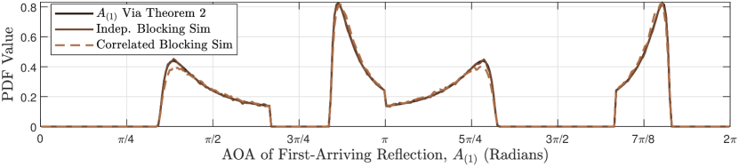
(a) Reflector orientations: $\textbf{Supp}(\Theta)=\{60^{\circ}\}$

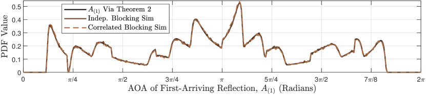
(b) Reflector orientations: $\textbf{Supp}(\Theta)=\{20^{\circ},40^{\circ},60^{\circ}\}$

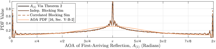
(c) Reflector orientations: $\textbf{Supp}(\Theta)=\{1^{\circ},5^{\circ},9^{\circ},\dots,81^{\circ},85^{\circ},89^{\circ}\}$

Figure 7: AOA Marginal PDFs of the 1${}^{\text{st}}$-Arriving Reflection. PDFs were generated for a test link setup of $d=350m$, a reflector density of $\lambda=30$ reflectors per $km^{2}$, reflector widths sampled from $f_{W}=\text{unif}(w_{min}=10m,w_{max}=40m,n_{w}=4)$, and reflector orientations given under each plot. Simulated PDFs were generated over 500,000 Boolean model realizations.

IV-A Numerical Results

This section compares our analytically derived AOA distribution of the first-arriving reflection (Theorem 2) against two AOA PDFs generated via simulation, labeled ‘Indep. Blocking Sim’ and ‘Correlated Blocking Sim’. The two simulated PDFs were generated in the exact same manner as in Sec. III-B, with the only difference being that the AOA of the first-arriving reflection was recorded rather than its path length. First, note the remarkable overlap between Theorem 2 and ‘Correlated Blocking Sim’ which reveals how well the independent blocking assumption holds. Next, the unique form of the distributions in Figs. 7(a) and 7(b) reveal that when reflectors take on one, or a few, orientations, such as buildings in a homogeneous city block for example, unique AOA profiles result, with certain AOAs being very prominent and others simply non-existent. This highlights how Theorem 2 can be used to optimize beam sweeping, for example, by greatly reducing the angular search space depending on the environment. Lastly, we compare Theorem 2 with an elliptical, omni-directional scattering model from the traditional channel modeling literature. The ‘AOA PDF’ from [18, Sec. V-B-2] in Fig. 7(c) was generated under the same base station-mobile separation distance, and assumes there is one omni-directional point scatterer uniformly distributed over an $s_{max}$-ellipse (see Def. 4), where $s_{max}$ was chosen s.t. $P[S_{(1)}\,|\,\{V_{\infty}\geq 1\}\leq s_{max}]\approx 0.75$, i.e., the analogous VRP associated with the first-arriving reflection in our model in Fig. 7(c) would fall within $\mathcal{E}_{s_{max}}$ $75\%$ of the time. It is fascinating to see that as we increase the number of reflector orientations, our AOA distribution in Theorem 2 begins to approach that of the omni-directional scattering model, with the notable exception being the pronounced peaks coming from both in front of and behind the mobile. To conclude, the distribution of $A_{(1)}$ presented here, derived under the Boolean model, is the first to capture the impact of environmental obstacles (i.e. buildings) at mm-wave frequencies, which is insight that can not be gleaned from the more elementary omni-directional scattering models where blocking, the Specular Reflection Law, and reflectors with non-zero area are not considered.

V Conclusion

Under a Boolean model of reflectors, which can facilitate or block reflections, and assuming NLOS propagation is due to first-order reflections, this paper presented the first analytical derivation of the TOA and AOA distributions of the first-arriving multipath component (MPC) experienced on a single link in outdoor, mm-wave (e.g., 5G) networks. In so doing, the TOA of the first-arriving MPC was used to derive the distribution of the bias experienced on NLOS range measurements for localization. It was shown that this analytically derived NLOS bias distribution: 1) matches closely with the decades-old exponential and gamma models assumed in the localization literature, thus offering the first support of these NLOS bias models based on the more accurate first-arriving MPC approach; and 2) gives intuition into how bias behaves when the environment of reflectors/blockages changes. Finally, numerical analysis of the AOA distribution revealed: 1) how reflector (e.g., building) orientations impact this distribution; and 2) how this distribution approaches the form of the AOA distribution of the first-arriving MPC from an elliptical, omni-directional scattering model as the number of reflector orientations increases.

Appendix A Proof Extension of Lemma 4: Convergence of Integrals in Intensity Measures

Here, we consider the worst case, i.e., $d=s_{1}$ and $s_{2}=\infty$, and show that the integrals in the following intensity measures converge:

$$\Lambda_{\text{I},v,w_{i},\theta_{j}}(\Omega_{\text{I}})=\!\frac{\lambda w_{i}}{n_{w}n_{\theta}}\!\int_{[\mathbf{R}_{\theta_{j}}\mathbf{m}]_{1}}^{\infty}\!\!\!\!\!\!\!\!\!\!\!\!\!\!\!\!\rho\Big{(}\mathbf{R}^{-1}_{\theta_{j}}\mathbf{g}^{*}_{\text{I}}(x_{\theta_{j}})\Big{)}\text{d}x_{\theta_{j}},~{}\,\Lambda_{\text{II},v,w_{i},\theta_{j}}(\Omega_{\text{II}})=\frac{\lambda w_{i}}{n_{w}n_{\theta}}\!\int_{[\mathbf{R}_{\theta_{j}}\mathbf{b}]_{2}}^{\infty}\!\!\!\!\!\!\!\!\!\!\!\!\!\!\!\rho\Big{(}\mathbf{R}^{-1}_{\theta_{j}}\mathbf{g}^{*}_{\text{II}}(y_{\theta_{j}})\Big{)}\,\text{d}y_{\theta_{j}}.$$ (12)

Consider first the integral in $\Lambda_{\text{I},v,w_{i},\theta_{j}}\!(\Omega_{\text{I}})$. We begin with two helpful derivations. The first is:

$$\mathbf{R}_{\theta_{j}}^{-1}\mathbf{g}^{*}_{\text{I}}(x_{\theta_{j}})=\big{(}4x_{\theta_{j}}\big{)}^{-1}\Big{[}(4x_{\theta_{j}}^{2}\!\!+\!d^{2}\!\sin^{2}\!\!\theta_{j})\cos\theta_{j},\,(4x_{\theta_{j}}^{2}\!\!-\!d^{2}\!\cos^{2}\!\!\theta_{j})\sin\theta_{j}\Big{]}^{T},$$ (13)

and the second is: $\rho(\mathbf{r})\stackrel{{\scriptstyle(a)}}{{=}}e^{-\frac{\lambda}{n_{w}n_{\theta}}\sum_{i=1}^{n_{w}}\sum_{j=1}^{n_{\theta}}\Big{[}\mu_{2}\big{(}\mathcal{L}_{[\mathbf{b},\mathbf{r}]}\oplus\mathcal{R}_{w_{i},\theta_{j}}\big{)}+\mu_{2}\big{(}\mathcal{L}_{[\mathbf{r},\mathbf{m}]}\oplus\mathcal{R}_{w_{i},\theta_{j}}\big{)}\Big{]}}$

$$\stackrel{{\scriptstyle(b)}}{{<}}e^{-\frac{\lambda}{n_{w}n_{\theta}}\sum_{i=1}^{n_{w}}\sum_{j=1}^{n_{\theta}}\big{[}w_{i}\lVert\mathbf{b}-\mathbf{r}\rVert+w_{i}\lVert\mathbf{r}-\mathbf{m}\rVert\big{]}}\stackrel{{\scriptstyle(c)}}{{<}}e^{-\frac{2\lambda\mathbb{E}[W]}{n_{\theta}}\sum_{j=1}^{n_{\theta}}\lVert\mathbf{r}-\mathbf{m}\rVert},$$ (14)

where (a) follows from Lemma 3 and Definition 2, (b) from Lemma 3 where we have that $\forall\mathbf{p},\mathbf{q}\in\mathbb{R}^{2},\mu_{2}\big{(}\mathcal{L}_{[\mathbf{p},\mathbf{q}]}\oplus\mathcal{R}_{w,\theta}\big{)}\geq w\lVert\mathbf{p}-\mathbf{q}\rVert+w^{2}>w\lVert\mathbf{p}-\mathbf{q}\rVert$, and (c) from $\mathbb{E}[W]=\Big{(}\sum_{i=1}^{n_{w}}w_{i}\Big{)}/n_{w}$ and from the fact that $\mathbf{r}\in Q_{\text{I}}\cup\{\mathbf{m}\}\implies\lVert\mathbf{r}-\mathbf{m}\rVert<\lVert\mathbf{b}-\mathbf{r}\rVert$.

Next, substituting (13) into (14) yields: $\rho\big{(}\mathbf{R}_{\theta_{j}}^{-1}\mathbf{g}^{*}_{\text{I}}(x_{\theta_{j}})\big{)}<$

$$\exp\left[-\frac{2\lambda\mathbb{E}[W]}{n_{\theta}}\sum_{j=1}^{n_{\theta}}\textstyle\sqrt{\!\left(\frac{\big{(}4x_{\theta_{j}}^{2}\!+d^{2}\sin^{2}\theta_{j}\big{)}\cos\theta_{j}}{4x_{\theta_{j}}}-\frac{d}{2}\right)^{2}\!\!\!+\frac{\big{(}4x_{\theta_{j}}^{2}\!-d^{2}\cos^{2}\theta_{j}\big{)}^{2}\!\!\sin^{2}\theta_{j}}{16x_{\theta_{j}}^{2}}}~{}\right].$$ (15)

The large square root term in the summand can be conveniently reduced to the following

$$\Bigg{(}x_{\theta_{j}}\!\!-\frac{d}{2}\cos\theta_{j}\Bigg{)}\sqrt{\!1\!+\frac{d^{2}\sin^{2}\!\theta_{j}}{4x_{\theta_{j}}^{2}}}\geq x_{\theta_{j}}\!\!-\frac{d}{2}\cos\theta_{j}$$ (16)

where the inequality follows from the fact that $\sqrt{1+(d^{2}\sin^{2}\!\theta_{j})/(4x_{\theta_{j}}^{2})}\geq 1$, since $x_{\theta_{j}}\geq(d/2)\cos\theta_{j}=[\mathbf{R}_{\theta_{j}}\mathbf{m}]_{1}$ (lower limit of integral in $\Lambda_{\text{I},v,w_{i},\theta_{j}}(\Omega_{\text{I}})$ in (12)).

Finally, substituting (16) in for the square root term in (15) and integrating both sides yields

$$\int_{[\mathbf{R}_{\theta_{j}}\mathbf{m}]_{1}}^{\infty}\!\!\!\!\!\!\!\!\!\!\!\!\!\!\!\!\rho\Big{(}\mathbf{R}^{-1}_{\theta_{j}}\mathbf{g}^{*}_{\text{I}}(x_{\theta_{j}})\Big{)}\text{d}x_{\theta_{j}}<\!\int_{[\mathbf{R}_{\theta_{j}}\mathbf{m}]_{1}}^{\infty}\!\!\!\!\!\!\!\!\!\!\!\!e^{-\frac{2\lambda\mathbb{E}[W]}{n_{\theta}}\sum_{j=1}^{n_{\theta}}\big{[}x_{\theta_{j}}-\frac{d}{2}\cos\theta_{j}\big{]}}\text{d}x_{\theta_{j}}=\frac{1}{2\lambda\mathbb{E}[W]},$$ (17)

and thus, the integral in $\Lambda_{\text{I},v,w_{i},\theta_{j}}(\Omega_{\text{I}})$ in (12) is bounded.

Following the same strategy, the integral in $\Lambda_{\text{II},v,w_{i},\theta_{j}}(\Omega_{\text{II}})$ in (12) can be shown to have the same bound as in (17). Thus, when $s_{2}=\infty$, $\Lambda_{\text{I},v,w_{i},\theta_{j}}(\Omega_{\text{I}})$ and $\Lambda_{\text{II},v,w_{i},\theta_{j}}(\Omega_{\text{II}})$ are bounded.

Appendix B Proof of Theorem 1

$$F_{S_{(1)}} (s_{(1)}\,|\,V_{\infty}\geq 1)=P[S_{(1)}\leq s_{(1)}\,|\,V_{\infty}\geq 1]=P[V_{s_{(1)}}\geq 1\,|\,V_{\infty}\geq 1]=\frac{P[V_{s_{(1)}}\geq 1,V_{\infty}\geq 1]}{P[V_{\infty}\geq 1]}$$

$$=\frac{P[V_{\infty}\geq 1\,|\,V_{s_{(1)}}\geq 1]\,P[V_{s_{(1)}}\geq 1]}{P[V_{\infty}\geq 1]}\stackrel{{\scriptstyle(a)}}{{=}}\frac{P[V_{s_{(1)}}\geq 1]}{P[V_{\infty}\geq 1]}\stackrel{{\scriptstyle(b)}}{{=}}\frac{1}{1-P[V_{\infty}=0]}\bigg{(}1-P[V_{s_{(1)}}=0]\bigg{)},$$

where (a) follows from $P[V_{\infty}\geq 1~{}|~{}V_{s_{(1)}}\geq 1]=1$, and (b) yields the CDF in the theorem since $V_{s_{(1)}}$ and $V_{\infty}$ are Poisson distributed according to Lemma 4.

The PDF is obtained by noting the following: $f_{S_{(1)}}(s_{(1)}|V_{\infty}\!\geq 1)=$

$$\frac{\partial}{\partial s_{(1)}}F_{S_{(1)}}(s_{(1)}\,|\,V_{\infty}\geq 1)\,=\,\frac{1}{1-e^{-\hat{\lambda}(\infty)}}e^{-\hat{\lambda}\big{(}s_{(1)}\big{)}}\frac{\partial}{\partial s_{(1)}}\Big{[}\hat{\lambda}\big{(}s_{(1)}\big{)}\Big{]}\stackrel{{\scriptstyle(a)}}{{=}}\frac{2\lambda\mathbb{E}[W]}{n_{\theta}\Big{(}1-e^{-\hat{\lambda}(\infty)}\Big{)}}e^{-\hat{\lambda}\big{(}s_{(1)}\big{)}}\times$$

$$\sum_{j=1}^{n_{\theta}}\!\Bigg{[}\!\rho\bigg{(}\!\mathbf{R}_{\theta_{j}}^{-1}\mathbf{g}_{\text{I}}^{*}\Big{(}\!\big{[}\mathbf{R}_{\theta_{j}}\mathbf{h}_{\text{I}}(s_{(1)}\!)\big{]}_{1}\Big{)}\!\bigg{)}\frac{\partial}{\partial s_{(1)}}\!\big{[}\mathbf{R}_{\theta_{j}}\mathbf{h}_{\text{I}}(s_{(1)}\!)\big{]}_{1}\!+\!\rho\bigg{(}\!\mathbf{R}_{\theta_{j}}^{-1}\mathbf{g}_{\text{II}}^{*}\Big{(}\!\big{[}\mathbf{R}_{\theta_{j}}\mathbf{h}_{\text{II}}(s_{(1)}\!)\big{]}_{2}\Big{)}\!\bigg{)}\frac{\partial}{\partial s_{(1)}}\!\big{[}\mathbf{R}_{\theta_{j}}\mathbf{h}_{\text{II}}(s_{(1)}\!)\big{]}_{2}\!\Bigg{]},$$

where (a) follows from Leibnitz’s Rule [34, Theorem 2.4.1]. Then, the PDF expression stated in the theorem is achieved from (a) via the following simplifications:

$$\rho\bigg{(}\mathbf{R}_{\theta_{j}}^{-1}\mathbf{g}_{\text{I}}^{*}\Big{(}\big{[}\mathbf{R}_{\theta_{j}}\mathbf{h}_{\text{I}}(s_{(1)})\big{]}_{1}\Big{)}\!\bigg{)}=\rho\big{(}\mathbf{h}_{\text{I},\theta_{j}}(s_{(1)})\big{)},~{}~{}~{}~{}~{}~{}~{}\rho\bigg{(}\mathbf{R}_{\theta_{j}}^{-1}\mathbf{g}_{\text{II}}^{*}\Big{(}\big{[}\mathbf{R}_{\theta_{j}}\mathbf{h}_{\text{II}}(s_{(1)})\big{]}_{2}\Big{)}\!\bigg{)}=\rho\big{(}\mathbf{h}_{\text{II},\theta_{j}}(s_{(1)})\big{)},$$

$$\frac{\partial}{\partial s_{(1)}}\big{[}\mathbf{R}_{\theta_{j}}\mathbf{h}_{\text{I}}(s_{(1)})\big{]}_{1}=\frac{s_{(1)}}{2\sqrt{s_{(1)}^{2}-d^{2}\sin^{2}\theta_{j}}},~{}~{}\text{and}~{}~{}~{}\frac{\partial}{\partial s_{(1)}}\big{[}\mathbf{R}_{\theta_{j}}\mathbf{h}_{\text{II}}(s_{(1)})\big{]}_{2}=\frac{s_{(1)}}{2\sqrt{s_{(1)}^{2}-d^{2}\cos^{2}\theta_{j}}},$$

where $\theta_{j}$ was added to $\mathbf{h}_{\text{I}}$, $\mathbf{h}_{\text{II}}$ to emphasize the dependence. The support follows from Def. 6.

Appendix C Proof of Theorem 2

$$f_{\!A_{(1)}}(\alpha_{(1)}\,|\,V_{\infty}\!\geq\!1)=\lim_{s_{max}\to\infty}\int_{d}^{s_{max}}\!\!\!\!\!\!\!\!f_{A_{(1)}}(\alpha_{(1)}\,|\,S_{(1)},V_{\infty}\geq 1)\,f_{S_{(1)}}(s_{(1)}\,|\,V_{\infty}\geq 1)\,\text{d}s_{(1)}$$

$$\stackrel{{\scriptstyle(a)}}{{=}}\sum\limits_{j=1}^{n_{\theta}}\sum\limits_{q\in\mathcal{Q}}\lim_{s_{max}\to\infty}\int_{d}^{s_{max}}\frac{\omega_{q,\theta_{j}}(s_{(1)})f_{S_{(1)}}(s_{(1)}\,|\,V_{\infty}\!\geq\!1)}{\sum_{j^{\prime}=1}^{n_{\theta}}\sum_{q^{\prime}\in\mathcal{Q}}\omega_{q^{\prime},\theta_{j^{\prime}}}(s_{(1)})}\delta\Big{(}\alpha_{(1)}-\psi_{q,\theta_{j}}(s_{(1)})\Big{)}\,\text{d}s_{(1)}$$

$$\stackrel{{\scriptstyle(b)}}{{=}}\sum\limits_{j=1}^{n_{\theta}}\sum\limits_{q\in\mathcal{Q}}\lim_{s_{max}\to\infty}\int_{\psi_{q,\theta_{j}}(d)}^{\psi_{q,\theta_{j}}(s_{max})}\frac{\Big{(}\psi_{q,\theta_{j}}^{-1}\Big{)}^{\prime}\!\!(\alpha)\,\omega_{q,\theta_{j}}\Big{(}\psi_{q,\theta_{j}}^{-1}(\alpha)\!\Big{)}f_{S_{(1)}}\Big{(}\psi_{q,\theta_{j}}^{-1}(\alpha)\,\Big{|}\,V_{\infty}\!\geq\!1\Big{)}}{\sum_{j^{\prime}=1}^{n_{\theta}}\sum_{q^{\prime}\in\mathcal{Q}}\omega_{q^{\prime},\theta_{j^{\prime}}}\Big{(}\psi_{q,\theta_{j}}^{-1}(\alpha_{(1)})\Big{)}}\delta\big{(}\alpha_{(1)}-\alpha\big{)}\,\text{d}\alpha,$$

where (a) follows from Lemma 6 and by finite additivity of limits and integrals, and (b) from the substitution: $\alpha=\psi_{q,\theta_{j}}(s_{(1)})\!\implies\!\psi_{q,\theta_{j}}^{-1}(\alpha)=s_{(1)}\!\implies\!\Big{(}\psi_{q,\theta_{j}}^{-1}\Big{)}^{\prime}\!(\alpha)\,\text{d}\alpha=\text{d}s_{(1)}$. The theorem follows by expanding the sum over $q\in\mathcal{Q}$, computing the integral limits via Table III, and computing the integrals by noting $\delta(\cdot)$ and the $\alpha_{(1)}$ values for which the integrals are non-zero.

References

- [1] C. E. O’Lone, H. S. Dhillon, and R. M. Buehrer, “A mathematical justification for exponentially distributed NLOS bias,” in Proc. of the IEEE Global Commun. Conf., Waikoloa, HI, USA, Dec. 2019, pp. 1-6.
- [2] S. N. Chiu, D. Stoyan, W. S. Kendall, and J. Mecke, Stochastic Geometry and its Applications, 3 ed., West Sussex, UK: Wiley, 2013.
- [3] T. Bai, R. Vaze, and R. W. Heath, “Analysis of blockage effects on urban cellular networks,” in IEEE Trans. on Wireless Commun., vol. 13, no. 9, pp. 5070-5083, Sept. 2014.
- [4] J. G. Andrews, T. Bai, M. N. Kulkarni, A. Alkhateeb, A. K. Gupta, and R. W. Heath, “Modeling and analyzing millimeter wave cellular systems,” in IEEE Trans. on Commun., vol. 65, no. 1, pp. 403-430, Jan. 2017.
- [5] N. A. Muhammad, P. Wang, Y. Li, and B. Vucetic, “Analytical model for outdoor millimeter wave channels using geometry-based stochastic approach,” in IEEE Trans. on Veh. Technol., vol. 66, no. 2, pp. 912-926, Feb. 2017.
- [6] R. T. Rakesh, G. Das, and D. Sen, “An analytical model for millimeter wave outdoor directional non-line-of-sight channels,” in Proc. of the IEEE Int. Conf. on Commun. (ICC), Paris, France, May 2017, pp. 1-6.
- [7] M. Dong and T. Kim, “Interference analysis for millimeter-wave networks with geometry-dependent first-order reflections,” in IEEE Trans. on Veh. Technol., vol. 67, no. 12, pp. 12404-12409, Dec. 2018.
- [8] C. E. O’Lone, H. S. Dhillon, and R. M. Buehrer, “Single-anchor localizability in 5G millimeter wave networks,” in IEEE Wireless Commun. Lett., vol. 9, no. 1, pp. 65-69, Jan. 2020.
- [9] A. Narayanan, S. T. Veetil, and R. K. Ganti, “Coverage analysis in millimeter wave cellular networks with reflections,” in Proc. of the IEEE Global Commun. Conf., Singapore, Dec. 2017, pp. 1-6.
- [10] Handbook of Position Location: Theory, Practice, and Advances, 2 ed., Wiley, Hoboken, NJ, 2019, pp. 224.
- [11] L. Cong and W. Zhuang, “Nonline-of-sight error mitigation in mobile location,” in IEEE Trans. on Wireless Commun., vol. 4, no. 2, pp. 560-573, Mar. 2005.
- [12] R. M. Vaghefi and R. M. Buehrer, “Cooperative sensor localization with NLOS mitigation using semidefinite programming,” in Proc. of the Workshop on Positioning, Navigation, and Commun., Dresden, Germany, Mar. 2012, pp. 13-18.
- [13] Y. Qi, H. Kobayashi, and H. Suda, “Analysis of wireless geolocation in a non-line-of-sight environment,” in IEEE Trans. on Wireless Commun., vol. 5, no. 3, pp. 672-681, Mar. 2006.
- [14] L. Mailaender, “On the geolocation bounds for round-trip time-of-arrival and all non-line-of-sight channels,” in EURASIP J. on Advances in Signal Process., vol. 2008, no. 1, pp. 1-10, Oct. 2007.
- [15] F. Yin, C. Fritsche, F. Gustafsson, and A. M. Zoubir, “TOA-based robust wireless geolocation and Cramér-Rao lower bound analysis in harsh LOS/NLOS environments,” in IEEE Trans. on Signal Process., vol. 61, no. 9, pp. 2243-55, May 2013.
- [16] S. Nawaz and N. Trigoni, “Robust localization in cluttered environments with NLOS propagation,” in Proc of the IEEE Int.l Conf. on Mobile Ad-hoc and Sensor Systems, San Fran., CA, USA, Nov. 2010, pp. 166-175.
- [17] Y. Qi and H. Kobayashi, “On geolocation accuracy with prior information in non-line-of-sight environment,” in Proc. of the IEEE 56th Veh. Technol. Conf., Vancouver, BC, Canada, Sept. 2002, pp. 285-288.
- [18] R. B. Ertel and J. H. Reed, “Angle and time of arrival statistics for circular and elliptical scattering models,” in IEEE J. Select. Areas in Commun., vol. 17, no. 11, pp. 1829-1840, Nov. 1999.
- [19] J.-F. Kiang and C.-W. Wu, “NLOS effects on position location techniques,” in IEEE Int. Conf. on Networking, Sensing and Control, Taipei, Taiwan, Mar. 2004, pp. 305-308
- [20] P. Chen, “A non-line-of-sight error mitigation algorithm in location estimation,” in Proc. of the IEEE Wireless Commun. and Networking Conf., New Orleans, LA, Sept. 1999, pp. 316-320.
- [21] S. Venkatesh, “The design and modeling of ultra-wideband position-location networks,” Ph.D Dissertation, Dept. of Elec. and Comp. Eng., Virginia Tech, Blacksburg, VA, 2007.
- [22] Y. Qi, H. Suda, and H. Kobayashi, “On time-of-arrival positioning in a multipath environment,” in Proc. of the IEEE 60th Veh. Technol. Conf.. Los Angeles, CA, USA, Sept. 2004, pp. 3540-3544.
- [23] Y. Li, J. G. Andrews, F. Baccelli, T. D. Novlan, and C. J. Zhang, “Design and analysis of initial access in millimeter wave cellular networks,” in IEEE Trans. on Wireless Commun., vol. 16, no. 10, pp. 6409-6425, Oct. 2017.
- [24] R. Janaswamy, “Angle and time of arrival statistics for the Gaussian scatter density model,” in IEEE Trans. on Wireless Commun., vol. 1, no. 3, pp. 488-497, July 2002.
- [25] S. Ju et al., “Scattering mechanisms and modeling for terahertz wireless communications,” in Proc. of the IEEE Int. Conf. on Commun. (ICC), Shanghai, China, May 2019, pp. 1-7.
- [26] A. A. AbdelNabi, V. Mancuso, and M. A. Marsan, “On the outage probability of millimeter wave links with quasi-deterministic propagation,” in Proc. of the 3 ACM Workshop on Millimeter-wave Networks and Sensing Systems, Los Cabos, Mexico, Oct. 2019, pp. 1-6.
- [27] S. Aditya, H. S. Dhillon, A. F. Molisch, and H. M. Behairy, “A tractable analysis of the blind spot probability in localization networks under correlated blocking,” in IEEE Trans. on Wireless Commun., vol. 17, no. 12, pp. 8150-64, Dec. 2018.
- [28] T. M. Cover and J. A. Thomas, Elements of Information Theory, ed. Hoboken, NJ, USA:Wiley, 2006.
- [29] M. P. Wylie and J. Holtzman, “The non-line of sight problem in mobile location estimation,” in Proc. of ICUPC - 5th Int. Conf. on Universal Personal Commun., Cambridge, MA, USA, Oct. 1996, pp. 827-831.
- [30] M. I. Silventoinen and T. Rantalainen, “Mobile station emergency locating in GSM,” in Proc. of the IEEE Int. Conf. on Personal Wireless Commun., New Delhi, India, Feb. 1996, pp. 232-238.
- [31] G. R. MacCartney and T. S. Rappaport, “A flexible millimeter-wave channel sounder with absolute timing,” in IEEE J. on Sel. Areas in Commun., vol. 35, no. 6, pp. 1402-1418, June 2017.
- [32] M. K. Samimi and T. S. Rappaport, “3-D millimeter-wave statistical channel model for 5G wireless system design,” in IEEE Trans. on Microwave Theory and Techn., vol. 64, no. 7, pp. 2207-2225, July 2016.
- [33] S. Ju, O. Kanhere, Y. Xing, and T. S. Rappaport, “A millimeter-wave channel simulator NYUSIM with spatial consistency and human blockage,” in Proc. of the IEEE Global Commun. Conf., Waikoloa, HI, USA, Dec. 2019, pp. 1-6.
- [34] G. Casella and R. L. Berger, Statistical Inference, ed. Belmont, CA, USA:Brooks/Cole, 2002.