Patterns and quasipatterns from the superposition of two hexagonal lattices

Abstract

When two-dimensional pattern-forming problems are posed on a periodic domain, classical techniques (Lyapunov–Schmidt, equivariant bifurcation theory) give considerable information about what periodic patterns are formed in the transition where the featureless state loses stability. When the problem is posed on the whole plane, these periodic patterns are still present. Recent work on the Swift–Hohenberg equation (an archetypal pattern-forming partial differential equation) has proved the existence of quasipatterns, which are not spatially periodic and yet still have long-range order. Quasipatterns may have 8-fold, 10-fold, 12-fold and higher rotational symmetry, which preclude periodicity. There are also quasipatterns with 6-fold rotational symmetry made up from the superposition of two equal-amplitude hexagonal patterns rotated by almost any angle $\alpha$ with respect to each other. Here, we revisit the Swift–Hohenberg equation (with quadratic as well as cubic nonlinearities) and prove existence of several new quasipatterns. The most surprising are hexa-rolls: periodic and quasiperiodic patterns made from the superposition of hexagons and rolls (stripes) oriented in almost any direction with respect to each other and with any relative translation; these bifurcate directly from the featureless solution. In addition, we find quasipatterns made from the superposition of hexagons with unequal amplitude (provided the coefficient of the quadratic nonlinearity is small). We consider the periodic case as well, and extend the class of known solutions, including the superposition of hexagons and rolls. While we have focused on the Swift–Hohenberg equation, our work contributes to the general question of what periodic or quasiperiodic patterns should be found generically in pattern-forming problems on the plane.

35B36, 37L10, 52C23

1 Introduction

Regular patterns are ubiquitous in nature, and carefully controlled laboratory experiments are capable of producing patterns, in the form of rolls (stripes), squares or hexagons, with an astonishingly high degree of symmetry. One particular example is the Faraday wave experiment, in which a layer of viscous fluid is subjected to sinusoidal vertical vibrations. Without the forcing, the surface of the fluid is flat and featureless, but as the strength of the forcing increases beyond a critical value, the flat surface loses stability to two-dimensional patterns of standing waves, which in simple cases take the form of roll, square or hexagonal patterns [2]. But, with more elaborate forcing, more complex patterns can be found. Figure 1 shows examples of (a,b) superlattice patterns and (c,d) quasipatterns [29, 2]. The images in (a,c) show the pattern of standing waves on the surface of the fluid, while (b,d) show the Fourier power spectra. In both cases, the patterns are dominated by twelve waves, indicated by twelve small circles in Figure 1(b) and by twelve blobs lying on a circle in Figure 1(d). The distance from the origin to the twelve peaks gives the wavenumber that dominates the pattern. In the superlattice example, the twelve peaks are unevenly spaced, but the basic structure is still hexagonal, and it is spatially periodic with a periodicity equal to $\sqrt{7}$ times the wavelength of the instability [29]. In the quasipattern example, spatial periodicity has been lost. Instead, the quasipattern has (on average) twelve-fold rotation symmetry, as seen in the repeating motif of twelve pentagons arranged in a circle and in the twelve evenly spaced peaks in the Fourier power spectrum in Fig. 1(d). The lack of spatial periodicity is apparent in Fig. 1(c), while the point nature of the power spectrum in Fig. 1(d) indicates that the pattern has long-range order. These two features, the lack of periodicity (implicit in this case from twelve-fold rotational symmetry) and the presence of long-range order, are characteristics of quasicrystals in metallic alloys [44] and soft matter [23], and in quasipatterns in fluid dynamics [18], reaction–diffusion systems [12] and optical systems [6].

The discovery of twelve-fold quasipatterns in the Faraday wave experiment [18] inspired a sequence of papers investigating this phenomenon [35, 55, 31, 38, 46, 41, 42, 47]. One of the main outcomes of this body of work is an understanding of the mechanism for stabilizing quasipatterns in Faraday waves. Twelve-fold quasicrystals have also been found in block copolymer and dendrimer systems [54, 23], in turn inspiring a considerable volume of work [4, 1, 8, 27, 48]. It turns out that the same stabilization mechanism operates in the Faraday wave and the polymer crystallization systems [30, 39]. In both cases, and indeed in other systems [12, 20], a common feature is that a second unstable or weakly damped length scale plays a key role in stabilizing the pattern. See [43] for a recent review.

(a) (b) (c) (d)

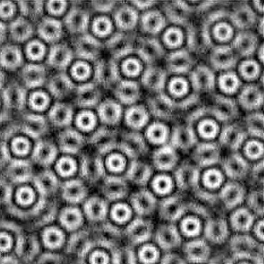
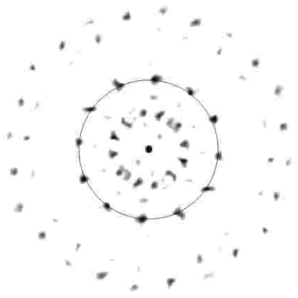
Figure 1: Examples of (a,b) superlattice patterns (reproduced with permission from [29]) and (c,d) quasipatterns (reproduced with permission from [2]). (a,c) show images representing the surface height of the fluid in Faraday wave experiments, with thin layers of viscous liquids subjected to large-amplitude multi-frequency forcing; (b,d) are Fourier power spectra of the images in (a,c), and indicate the twelve peaks that dominate the patterns in each case.

However, as well the question of how superlattice patterns and quasipatterns are stabilized, there is the question of their existence as solutions of pattern-forming partial differential equations (PDEs) posed on the plane, without lateral boundaries [26, 5, 10, 9]. Superlattice patterns, which have spatial periodicity (as in Fig. 1a) can be analysed in finite domains with periodic boundary conditions. In this case, and near the bifurcation point, spatially periodic patterns have Fourier expansions with wave vectors that live on a lattice, and the infinite-dimensional PDE can be reduced rigorously to a finite-dimensional set of equations for the amplitudes of the primary modes [11, 51]. In the finite dimensional setting, amplitude equations can be written down, bifurcating equilibrium points found and their stability analysed [15]. Equivariant bifurcation theory [21] is a powerful tool that uses symmetry techniques to prove existence of certain classes of symmetric periodic patterns without recourse to amplitude equations.

But quasipatterns pose a particular challenge for proving existence, in that the formal power series that describes small amplitude solutions may diverge [40, 26] owing to the appearance of small divisors. Nonetheless, existence of quasipatterns with $Q$-fold rotation symmetry ($Q=8$, $10$, $12$, …) as solutions of the steady Swift–Hohenberg equation (see below) has been proved using methods based on the Nash–Moser theorem [10]. The same approach has been applied to other pattern-forming PDEs, such as those for steady Bénard–Rayleigh convection [9]. Throughout, the existence proofs show that as the amplitude of the quasipattern solution goes to zero, the solution from the truncated formal expansion approaches a quasipattern solution of the PDE in a union of disjoint parameter intervals, going to full measure as the amplitude goes to zero.

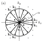
Figure 2: (a) Two sets of six equally spaced wave vectors (${\mathbf{k}}_{1}$, ${\mathbf{k}}_{2}$, ${\mathbf{k}}_{3}$ and their opposites, and ${\mathbf{k}}_{4}$, ${\mathbf{k}}_{5}$, ${\mathbf{k}}_{6}$ and their opposites) rotated an angle $\alpha$ with respect to each other so as to produce spatially periodic patterns: $\alpha\approx 21.79^{\circ}$, with $\cos\alpha=\frac{13}{14}$ and $\sqrt{3}\sin\alpha=\frac{9}{14}$. The gray dots indicate that the twelve vectors lie on an underlying hexagonal lattice, generated by the vectors ${\mathbf{s}}_{1}$ and ${\mathbf{s}}_{2}$. Compare with Fig. 1(b). (b) 12-fold quasipatterns are generated by twelve equally spaced vectors: $\alpha=\frac{\pi}{6}=30^{\circ}$, with $\cos\alpha=\frac{1}{2}\sqrt{3}$. Compare with Fig. 1(d). (c) 6-fold quasiperiodic case: $\alpha\approx 25.66^{\circ}$, with $\cos\alpha=\frac{1}{4}\sqrt{13}$ and $\sqrt{3}\sin\alpha=\frac{3}{4}$. Quasipatterns generated by equal combinations of the twelve waves have six-fold rotation symmetry but lack spatial periodicity.

Most previous work on quasipatterns has concentrated on Fourier spectra that exhibit “prohibited” symmetries: eight-, ten-, twelve-fold and higher rotation symmetries, as in Fig. 1(c), or icosahedral symmetry in three dimensions [48]. There is, however, a class of quasipatterns with six-fold rotation symmetry, related to the superlattice patterns already discussed. These patterns can be described in terms of the superposition of twelve waves with twelve wavevectors, grouped into two sets of six as in Fig. 2, with the six vectors within each set spaced evenly around the circle, and with the two sets rotated by an angle $\alpha$ with respect to each other, with $0<\alpha<\frac{\pi}{3}$. In the quasiperiodic case, we can choose $\alpha$ to be the smallest angle between the vectors, so $0<\alpha\leq\frac{\pi}{6}$.

The discovery, in the Faraday wave experiment and elsewhere, of these elaborate superlattice patterns and quasipatterns, with and without spatial periodicity, motivated investigations into the bifurcation structure of pattern formation problems posed both in periodic domains and on the whole plane, without lateral boundaries. We focus on an example of such a problem, the steady Swift–Hohenberg equation, which is:

(1) $$(1+\Delta)^{2}u-\mu u+\chi u^{2}+u^{3}=0,$$

where $u({\mathbf{x}})$ is a real function of ${\mathbf{x}}=(x,y)\in\mathbb{R}^{2}$, $\Delta$ is the Laplace operator, $\mu$ is a real bifurcation parameter and $\chi$ is a real parameter. The time-dependent version of this PDE was proposed originally as a model of small-amplitude fluctuations near the onset of convection [50], but is now considered an archetypal model of pattern formation [24].

The trivial state $u=0$ is always a solution of Eq. 1, and as $\mu$ increases through zero, many branches of small-amplitude solutions of Eq. 1 are created. These include periodic patterns such as rolls, squares, hexagons and superlattice patterns, quasipatterns with the prohibited rotation symmetries of eight-, ten-, twelve-fold and higher (proved in [10] with $\chi=0$), as well as (again with $\chi=0$) two families of six-fold quasipatterns with equal sums of the twelve Fourier modes illustrated in Fig. 2(c) [25, 19]. In this paper, we extend the analysis in [25] by allowing $\chi\neq 0$ and including quasipatterns with unequal combinations of the twelve Fourier modes, discovering several new classes of solutions.

We approach this problem by deriving nonlinear amplitude equations for the twelve Fourier modes on the unit circle. One important requirement on the twelve selected modes illustrated in Fig. 2 is therefore that nonlinear combinations of these modes should generate no further modes with wavevectors on the unit circle. If they did, additional amplitude equations would have to be included, a problem we leave for another day. We call the (full measure, as proved in [25] in Lemma 5) set of $\alpha$’s that satisfy this condition ${\mathcal{E}_{0}}$, defined more precisely in [25] and in Definition 2.4 below. Throughout, we use the names of the sets of values of $\alpha$ from [25].

There are three possible situations as $\alpha$ is varied: the (zero measure) periodic case, the (full measure) quasiperiodic case where the results of [25] can be used, and other quasiperiodic values of $\alpha$ (zero measure). See the definitions below and in Appendix A for more detail.

1. The lattice is periodic, and $\alpha\in{\mathcal{E}_{p}}$, as in Fig. 2(a) (see Definition 2.1). For these angles, restricted to $0<\alpha<\frac{\pi}{3}$, both $\cos\alpha$ and $\sqrt{3}\sin\alpha$ must be rational, and the wave vectors generate a lattice (see Definition 2.1 and Lemma 2.2 below). This is the case examined by [15], and $\alpha\approx 21.79^{\circ}$ ($\cos\alpha=\frac{13}{14}$ and $\sqrt{3}\sin\alpha=\frac{9}{14}$) is an example. For reasons explained below, for some values of $\alpha\in{\mathcal{E}_{p}}$, is it more convenient to consider $\frac{\pi}{3}-\alpha$ instead, relabelling the vectors. This set is dense but of measure zero. Not all values of $\alpha\in{\mathcal{E}_{p}}$ are also in ${\mathcal{E}_{0}}$.

2. The angle $\alpha$ is not in ${\mathcal{E}_{p}}$ but it satisfies all three of the requirements for the existence proofs in [25]. The first requirement is that $\alpha\in{\mathcal{E}_{0}}$ (see Definition 2.4 below): no integer combination of the twelve vectors already chosen should lie on the unit circle apart from the twelve. The second and third requirements are that the numbers $\cos\alpha$ and $\sqrt{3}\sin\alpha$ should satisfy two “good” Diophantine properties. We define ${\mathcal{E}_{1}}$ and ${\mathcal{E}_{2}}$ to be the set of such angles, restricted to $0<\alpha\leq\frac{\pi}{6}$ (see definitions in Appendix A). Then, the set ${\mathcal{E}_{2}}$, which itself requires ${\mathcal{E}_{0}}$ and ${\mathcal{E}_{1}}$, is the set of angles that satisfy all three requirements. All rational multiples of $\pi$ (restricted to $0<\alpha\leq\frac{\pi}{6}$) are in ${\mathcal{E}_{2}}$, for example, $\alpha=\frac{\pi}{6}=30^{\circ}$ as in Fig. 2(b). The angle $\alpha\approx 25.66^{\circ}$ is another example, ($\cos\alpha=\frac{1}{4}\sqrt{13}$ and $\sqrt{3}\sin\alpha=\frac{3}{4}$, see Fig. 2(c) and Appendix B). This set is of full measure.

3. The angle $\alpha$, still restricted to $0<\alpha\leq\frac{\pi}{6}$, is not in ${\mathcal{E}_{p}}$ or ${\mathcal{E}_{2}}$, and although patterns made from these modes may be quasiperiodic, the existence proofs based on the approach of [25] do not work, at least not without further extension. The angle $\alpha\approx 26.44^{\circ}$ ($\cos\alpha=\frac{1}{12}(5+\sqrt{33})$ and $\sqrt{3}\sin\alpha=\frac{1}{12}(15-\sqrt{33})$) is an example (see Appendix B) since it is not in ${\mathcal{E}_{0}}$. This set is dense but of measure zero.

For $\alpha\in{\mathcal{E}_{p}}\cap{\mathcal{E}_{0}}$, the resulting superlattice patterns are spatially periodic, and their bifurcation structure is determined at finite order when the small amplitude pattern is expressed as a formal power series [15]. The wavevectors for these spatially periodic superlattice patterns lie on a finer hexagonal lattice (as in Fig. 2a).

We define ${\mathcal{E}_{qp}}$ to be the complement of ${\mathcal{E}_{p}}$ restricted to $0<\alpha\leq\frac{\pi}{6}$. For $\alpha\in{\mathcal{E}_{qp}}$, linear combinations of waves are typically quasiperiodic, but only for $\alpha\in{\mathcal{E}_{2}}\subset{\mathcal{E}_{qp}}$ can the techniques of [25] be used to prove existence of quasipatterns with these modes as nonlinear solutions of the PDE Eq. 1. For the special case $\alpha=\frac{\pi}{6}\in{\mathcal{E}_{2}}$, as in Fig. 2(b), the quasipattern has twelve-fold rotation symmetry, but more generally, as in Fig. 2(c), there can be six-fold rotation symmetry, more usually associated with hexagons. The proof in [25] makes use of the properties of ${\mathcal{E}_{2}}$; at this time, no existence result is known about $\alpha\notin{\mathcal{E}_{2}}\cup{\mathcal{E}_{p}}$.

The periodic case has been analysed by [15, 45]. They write the small-amplitude pattern $u({\mathbf{x}})$ as the sum of six complex amplitudes $z_{1}$, …, $z_{6}$ times the six waves $e^{i{\mathbf{k}}_{1}\cdot{\mathbf{x}}}$, …, $e^{i{\mathbf{k}}_{6}\cdot{\mathbf{x}}}$:

(2) $$u({\mathbf{x}})=\sum_{j=1}^{6}z_{j}e^{i{\mathbf{k}}_{j}\cdot{\mathbf{x}}}+c.c.+\text{high-order terms},$$

where $c.c.$ refers to the complex conjugate, and the six wavevectors ${\mathbf{k}}_{1}$, …, ${\mathbf{k}}_{6}$ are as illustrated in Fig. 2(a). They then derive, using symmetry considerations, the amplitude equations:

(3) $$\begin{split}0&=z_{1}f_{1}(u_{1},\dots,u_{6},q_{1},q_{4},{\bar{q}}_{4})+{\bar{z}}_{2}{\bar{z}}_{3}f_{2}(u_{1},\dots,u_{6},{\bar{q}}_{1},q_{4},{\bar{q}}_{4})+{}\\ &\qquad{}+\text{high-order resonant terms},\end{split}$$

where $u_{1}=|z_{1}|^{2}$, …, $u_{6}=|z_{6}|^{2}$, $q_{1}=z_{1}z_{2}z_{3}$, and $q_{4}=z_{4}z_{5}z_{6}$. Here, $f_{1}$ and $f_{2}$ are smooth functions of their nine arguments. Five additional equations can be deduced from permutation symmetry. The high-order resonant terms, present only in the periodic case, are at least fifth order polynomial functions of the six amplitudes and their complex conjugates, and depend on the choice of $\alpha\in{\mathcal{E}_{p}}$. Even without the amplitude equations Eq. 3, equivariant bifurcation theory can be used [21, 15] to deduce the existence of various hexagonal and triangular superlattice patterns, and, within the amplitude equations, the stability of these patterns can be computed.

The approach we take does not use equivariant bifurcation theory. Instead, we derive amplitude equations of the form Eq. 3 in the quasiperiodic and periodic cases. In the quasiperiodic case, the equation is a formal power series, but in both cases, the cubic truncation of the first component of amplitude equations is of the form

(4) $$0=\mu z_{1}-\alpha_{0}{\bar{z}}_{2}{\bar{z}}_{3}-z_{1}(\alpha_{1}u_{1}+\alpha_{2}u_{2}+\alpha_{2}u_{3}+\alpha_{4}u_{4}+\alpha_{5}u_{5}+\alpha_{6}u_{6}),$$

where $\alpha_{0}$, …, $\alpha_{6}$ are coefficients that can be computed from the PDE Eq. 1. We find small amplitude solutions of the cubic truncation Eq. 4 then verify that these correspond to small amplitude solutions of the untruncated amplitude equations Eq. 3. One remarkable result is that the formal expansion in powers of the amplitude (and parameter $\chi$ in the cases when $\chi$ is close to 0) of the bifurcating patterns is given at leading order by the same formulae in both the quasiperiodic and the periodic cases. From solutions of the amplitude equations, the mathematical proof of existence of the periodic patterns is given by the classical Lyapunov–Schmidt method, while for quasipatterns the proof follows the same lines as in [25]. The truncated expansion of the formal power series provides the first approximation to the quasipattern solution, which is a starting point for the Newton iteration process, using the Nash–Moser method for dealing with the small divisor problem [25] (for more details see §4.2.1).

Name	Section Figure	Periodic or QP	Example amplitudes	$\chi$	Earlier results
QP-super- hexagons	§4.2.1 Fig. 4	QP	$z_{1}=\dots=z_{6}\in\mathbb{R}$	Any	[25]
Unequal QP-super- hexagons	§4.2.1 Fig. 4	QP	$z_{1}=z_{2}=z_{3}\neq{}$ $z_{4}=z_{5}=z_{6}\in\mathbb{R}$	$|\chi|\ll 1$	New
QP-anti-hexagons, QP-triangles etc.	§4.2.1 Fig. 5	QP	Various: see Eq. 21	$\chi=0$	New
Super- hexagons	§4.2.2 Fig. 6	Periodic	$z_{1}=\dots=z_{6}\in\mathbb{R}$	Any	[15]
Triangular superlattice	§4.2.2 Fig. 6	Periodic	Equal amplitudes $\mbox{Phases}\approx\frac{\pi}{3},\frac{2\pi}{3}$	Any	[45]
Hexa-rolls (rolls dominant)	§4.3.1 Fig. 7	QP and periodic	$z_{1}\approx z_{2}\approx z_{3}\ll z_{4}$, $z_{5}=z_{6}=0$	$\chi$ neither too small nor too large	New
Hexa-rolls (balanced)	§4.3.2 Fig. 7	QP and periodic	$z_{1}\approx z_{2}\approx z_{3}\sim z_{4}$, $z_{5}=z_{6}=0$	$|\chi|\ll 1$	New

Table 1: Summary of the different solutions we consider. “Periodic” and “QP” refer to periodic ($\alpha\in{\mathcal{E}_{p}}\cap{\mathcal{E}_{0}}$) and quasiperiodic ($\alpha\in{\mathcal{E}_{2}}$) respectively. We give examples of the six $z_{j}$ amplitudes as well as restrictions on the values of $\chi$. The term “super-hexagon” refers to the superposition of two hexagonal patterns, which can be equal or unequal amplitude. The last column gives references to relevant earlier results or indicates whether the solutions are new.

We find several new types of solution, in the quasiperiodic and in the periodic cases, and in the $\chi\neq 0$ and $|\chi|\ll 1$ cases. These are summarized in Table 1. The most significant new class of solutions is the superposition of hexagons and roll patterns (hexa-rolls), with the rolls arranged at almost any orientation with respect to the hexagons ($\alpha\in({\mathcal{E}_{p}}\cup{\mathcal{E}_{2}})\cap{\mathcal{E}_{0}}$) and translated with respect to each other by arbitrary amounts. These bifurcate directly from the featureless pattern even when $\chi$ is not small (provided $\chi$ is not too large, see §4.3.1), in both the periodic and the quasiperiodic cases. In the quasiperiodic case, the phason symmetry [17] characteristic of quasipatterns leads to the freedom to have arbitrary relative translations of the hexagons and rolls; finding this same freedom in the periodic case was a surprise.

We also show that the particular example of periodic triangular superlattice patterns reported experimentally in [29] (see Fig. 1a) and explored theoretically in [45] can also be found in a much wider class of periodic lattices. Moreover, for nearby angles $\alpha\in{\mathcal{E}_{2}}$, we find that the quasiperiodic super-hexagons can be thought of as long-range modulations between the periodic super-hexagons and two types of periodic superlattice triangles (see Fig. 6).

Our work extends the periodic results of [15] to the quasiperiodic case, including quasiperiodic versions of the anti-hexagon, super-triangle and anti-triangle patterns that occur with $\chi=0$. We also extend the previous quasiperiodic work of [19, 25], which took $\chi=0$: we find small-amplitude bifurcating solutions in Eq. 3 for any $\chi\neq 0$, including new quasiperiodic superposed hexagon patterns with unequal amplitudes for $0<|\chi|\ll 1$, and show that there are corresponding quasiperiodic (and periodic) solutions of the Swift–Hohenberg equation.

Amongst the solutions we find in the quasiperiodic case are combinations of two hexagonal patterns, as well as the hexa-roll patterns mentioned above. In both the periodic and the quasiperiodic cases, the superposed hexagon and roll patterns are new, and would not be found using the equivariant bifurcation lemma as they have no symmetries (beyond periodic in that case). Also in both cases, we consider the possibility that $\chi$ is small, and use the method of [25] on power series in two small parameters to find new superposed hexagon patterns with unequal amplitudes, again out of range of the equivariant bifurcation lemma.

We open the paper with a statement of the problem in Section 2 and develop the formal power series for the amplitude equations in Section 3. We solve these equations in Section 4, focusing on the new solutions, and conclude in Section 5. Some details of the definitions, examples and proofs are in the six appendices.

2 Statement of the problem

We begin by explaining how we describe functions on lattices and quasilattices, and how the symmetries of the problem act on these functions.

2.1 Lattices and quasilattices

In the Fourier plane, we have two sets of six basic wave vectors as illustrated in Fig. 2: $\{{\mathbf{k}}_{j},-{\mathbf{k}}_{j}:j=1,2,3\}$ and $\{{\mathbf{k}}_{j},-{\mathbf{k}}_{j}:j=4,5,6\}$, both equally spaced on the unit circle, with angle $\frac{2\pi}{3}$ between ${\mathbf{k}}_{1}$, ${\mathbf{k}}_{2}$ and ${\mathbf{k}}_{3}$ and between ${\mathbf{k}}_{4}$, ${\mathbf{k}}_{5}$ and ${\mathbf{k}}_{6}$, such that ${\mathbf{k}}_{1}+{\mathbf{k}}_{2}+{\mathbf{k}}_{3}=0$ and ${\mathbf{k}}_{4}+{\mathbf{k}}_{5}+{\mathbf{k}}_{6}=0$. The two sets of six vectors are rotated by an angle $\alpha$ ($0<\alpha<\frac{\pi}{3}$) with respect to each other, so that ${\mathbf{k}}_{1}$ makes an angle $-\alpha/2$ with the $x$ axis, while ${\mathbf{k}}_{4}$ makes an angle $\alpha/2$ with the $x$ axis. The case $\alpha=\frac{\pi}{6}$ corresponds to the situation 12-fold quasipattern treated in [10], though with $\chi=0$.

The lattice (in the periodic case) or quasilattice $\Gamma$ are made up of integer sums of the six basic wave vectors:

(5) $$\Gamma=\left\{{\mathbf{k}}\in\mathbb{R}^{2}:{\mathbf{k}}=\sum_{j=1}^{6}m_{j}{\mathbf{k}}_{j},\quad\text{with}\quad m_{j}\in\mathbb{Z}\right\}.$$

Notice that if ${\mathbf{k}}\in\Gamma$ then $-{\mathbf{k}}\in\Gamma$. In the periodic case, the lattice is not dense, as in Fig. 2(a), while in the quasiperiodic case, the points in $\Gamma$ are dense in the plane.

The periodic case occurs whenever the two sets of six wave vectors are not rationally independent, meaning that, for example, ${\mathbf{k}}_{4}$, ${\mathbf{k}}_{5}$ and ${\mathbf{k}}_{6}$ can all be written as rational sums of ${\mathbf{k}}_{1}$ and ${\mathbf{k}}_{2}$. This happens whenever $\cos\alpha$ and $\cos(\alpha+\frac{\pi}{3})$ are both rational, and in this case, patterns defined by Eq. 2 are periodic in space. We define the set ${\mathcal{E}_{p}}$ to be these angles.

Definition 2.1.

Periodic case: the set ${\mathcal{E}_{p}}$ of angles is defined as

$${\mathcal{E}_{p}}:=\left\{\alpha\in\left(0,\frac{\pi}{3}\right):\cos\alpha\in\mathbb{Q}\quad\text{\rm and}\quad\cos\left(\alpha+\frac{\pi}{3}\right)\in\mathbb{Q}\right\}.$$

In this case, $\Gamma$ is a lattice with hexagonal symmetry. We can replace $\cos(\alpha+\frac{\pi}{3})$ in this definition by $\sqrt{3}\sin\alpha$. The set ${\mathcal{E}_{p}}$ has the following properties:

Lemma 2.2.

(i) The set ${\mathcal{E}_{p}}$ is dense and has zero measure in $(0,\frac{\pi}{3})$.

(ii) If the wave vectors ${\mathbf{k}}_{1}$, ${\mathbf{k}}_{2}$, ${\mathbf{k}}_{4}$ and ${\mathbf{k}}_{5}$ are not independent on $\mathbb{Q}$, then $\alpha\in{\mathcal{E}_{p}}$.

(iii) If $\alpha\in{\mathcal{E}_{p}}$ then there exist co-prime integers $a,b$ such that

$$a>b>\frac{a}{2}>0,\quad a\geq 3,\quad\text{$a+b$ not a multiple of 3},$$

(6) $$\cos\alpha=\frac{a^{2}+2ab-2b^{2}}{2(a^{2}-ab+b^{2})},\quad\sqrt{3}\sin\alpha=\frac{3a(2b-a)}{2(a^{2}-ab+b^{2})}.$$

Then the wave vectors ${\mathbf{k}}_{j}$ are integer combinations of two smaller vectors ${\mathbf{s}}_{1}$ and ${\mathbf{s}}_{2}$, of equal length $\lambda=(a^{2}-ab+b^{2})^{-1/2}$, making an angle of $\frac{2\pi}{3}$, with

(7) $${\mathbf{k}}_{1} =a{\mathbf{s}}_{1}+b{\mathbf{s}}_{2},\quad {\mathbf{k}}_{2} =(b-a){\mathbf{s}}_{1}-a{\mathbf{s}}_{2},\quad {\mathbf{k}}_{3} =-b{\mathbf{s}}_{1}+(a-b){\mathbf{s}}_{2},$$

$${\mathbf{k}}_{4} =a{\mathbf{s}}_{1}+(a-b){\mathbf{s}}_{2},\quad {\mathbf{k}}_{5} =-b{\mathbf{s}}_{1}-a{\mathbf{s}}_{2},\quad {\mathbf{k}}_{6} =(b-a){\mathbf{s}}_{1}+b{\mathbf{s}}_{2}.$$

Part (ii) of the Lemma is proved in [25], and parts (i) and (iii) are proved in Appendix C. The vectors ${\mathbf{s}}_{1}$ and ${\mathbf{s}}_{2}$ are illustrated in Fig. 2 in the case $(a,b)=(3,2)$ with $\lambda=1/\sqrt{7}$. Requiring $a+b$ not to be a multiple of 3 means that we need to allow $0<\alpha<\frac{\pi}{3}$ in the periodic case. In the quasiperiodic case ($\alpha\in{\mathcal{E}_{qp}}$), we can always take $\alpha$ to be the smallest of the angles between the vectors, which is why we define the set ${\mathcal{E}_{qp}}$ to be the complement of ${\mathcal{E}_{p}}$ within the interval $(0,\frac{\pi}{6}]$.

In Eq. 5, vectors ${\mathbf{k}}\in\Gamma$ are indexed by six integers ${\mathbf{m}}=(m_{1},\dots,m_{6})\in\mathbb{Z}^{6}$. However, using the fact that ${\mathbf{k}}_{1}+{\mathbf{k}}_{2}+{\mathbf{k}}_{3}=0$ and ${\mathbf{k}}_{4}+{\mathbf{k}}_{5}+{\mathbf{k}}_{6}=0$, the set $\Gamma$ can be indexed by fewer than six integers, and any ${\mathbf{k}}\in\Gamma$ may be written, in both the periodic and the quasiperiodic cases, as

(8) $${\mathbf{k}}({\mathbf{m}})=m_{1}{\mathbf{k}}_{1}+m_{2}{\mathbf{k}}_{2}+m_{4}{\mathbf{k}}_{4}+m_{5}{\mathbf{k}}_{5},\quad(m_{1},m_{2},m_{4},m_{5})\in\mathbb{Z}^{4},$$

though in fact $\Gamma$ is indexed by two integers in the periodic case $\alpha\in{\mathcal{E}_{p}}$.

2.2 Functions on the (quasi)lattice

We are now in a position to specify more precisely the form of the sum in Eq. 2. The function $u({\mathbf{x}})$ is a real function that we write in the form of a Fourier expansion with Fourier coefficients $u^{({\mathbf{k}})}$:

(9) $$u({\mathbf{x}})=\sum_{{\mathbf{k}}\in\Gamma}u^{({\mathbf{k}})}e^{i{\mathbf{k}}\cdot{\mathbf{x}}},\quad u^{({\mathbf{k}})}={\bar{u}}^{(-{\mathbf{k}})}\in\mathbb{C}.$$

With ${\mathbf{k}}\in\Gamma$ written as in Eq. 8, in the quasiperiodic case ($\alpha\in{\mathcal{E}_{qp}}$) four indices are needed in the sum since the four vectors in Eq. 8 are rationally independent. In the periodic case, two indices are needed. A norm $N_{{\mathbf{k}}}$ for $\alpha\in{\mathcal{E}_{qp}}$ is defined by

$$N_{{\mathbf{k}}(\mathbf{m})}=|m_{1}|+|m_{2}|+|m_{4}|+|m_{5}|=|\mathbf{m}|,$$

where the coefficients $m_{j}$ are uniquely defined for a given vector ${\mathbf{k}}\in\Gamma$. To give a meaning to the above Fourier expansion we need to introduce Hilbert spaces $\mathcal{H}_{s}$, $s\geq 0:$

$$\mathcal{H}_{s}=\left\{u=\sum_{{\mathbf{k}}\in\Gamma}u^{({\mathbf{k}})}e^{i{\mathbf{k}}\cdot{\mathbf{x}}};\quad u^{({\mathbf{k}})}=\overline{u}^{(-{\mathbf{k}})}\in\mathbb{C},\quad\sum\limits_{{\mathbf{k}}\in\Gamma}|u^{({\mathbf{k}})}|^{2}(1+N_{{\mathbf{k}}}^{2})^{s}<\infty\right\},$$

It is known that $\mathcal{H}_{s}$ is a Hilbert space with the scalar product

$$\langle u,v\rangle_{s}=\sum_{{\mathbf{k}}\in\Gamma}(1+N_{{\mathbf{k}}}^{2})^{s}u^{({\mathbf{k}})}\overline{v}^{({\mathbf{k}})},$$

and that $\mathcal{H}_{s}$ is an algebra for $s>2$ (see [10]), and possesses properties of Sobolev spaces $H_{s}$ in dimension 4, for example $u$ is of class $C^{l}$ for $s>l+2$. For $\alpha\in{\mathcal{E}_{qp}}$, a function in $\mathcal{H}_{s}$, defined by a convergent Fourier series as in Eq. 9, represents in general a quasipattern, i.e., a function that is quasiperiodic in all directions. It is possible of course for such functions still to be periodic (e.g., rolls or hexagons) if subsets of the Fourier amplitudes are zero. With this definition of the scalar product, the twelve basic modes are orthogonal in $\mathcal{H}_{s}$ and orthonormal in $\mathcal{H}_{0}$:

$$\left\langle e^{i{\mathbf{k}}_{j}\cdot{\mathbf{x}}},e^{i{\mathbf{k}}_{l}\cdot{\mathbf{x}}}\right\rangle_{0}=\left\langle e^{-i{\mathbf{k}}_{j}\cdot{\mathbf{x}}},e^{-i{\mathbf{k}}_{l}\cdot{\mathbf{x}}}\right\rangle_{0}=\delta_{j,l}\quad\text{and}\quad\left\langle e^{\pm{i}{\mathbf{k}}_{j}\cdot{\mathbf{x}}},e^{\mp i{\mathbf{k}}_{l}\cdot{\mathbf{x}}}\right\rangle_{0}=0,$$

where $\delta_{j,l}$ is the Kronecker delta.

The following useful Lemma is proven in [25]:

Lemma 2.3.

For nearly all $\alpha\in(0,\frac{\pi}{6}]$, and in particular for $\alpha\in\mathbb{Q}\pi\cap(0,\frac{\pi}{6}]$, the only solutions of $|{\mathbf{k}}({\mathbf{m}})|=1$ are $\pm{\mathbf{k}}_{j}$, $j=1,\dots,6$. These vectors can be expressed with four integers as in Eq. 8:

$${\mathbf{m}}=(\pm 1,0,0,0),(0,\pm 1,0,0),(0,0,\pm 1,0),(0,0,0,\pm 1),\pm(1,1,0,0),\pm(0,0,1,1).$$

For these values of $\alpha$, the only vectors in $\Gamma$ that are on the unit circle are the original twelve vectors, defining the set ${\mathcal{E}_{0}}$:

Definition 2.4.

${\mathcal{E}_{0}}$ is the set of $\alpha$’s such that Lemma 2.3 applies: the set of $\alpha\in(0,\frac{\pi}{6}]$ such that the only solutions of $|{\mathbf{k}}({\mathbf{m}})|=1$ are $\pm{\mathbf{k}}_{j}$, $j=1,\dots,6$.

The set ${\mathcal{E}_{0}}$ is dense and of full measure in $(0,\frac{\pi}{6}]$ (see [25], proof of Lemma 5), and contains angles $\alpha\in{\mathcal{E}_{p}}$ and $\alpha\in{\mathcal{E}_{qp}}$. Not every $\alpha\in{\mathcal{E}_{p}}$ is also in ${\mathcal{E}_{0}}$; for example, if $(a,b)=(8,5)$, we have $3{\mathbf{k}}_{1}+{\mathbf{k}}_{2}-2{\mathbf{k}}_{4}+{\mathbf{k}}_{5}=(5b-4a){\mathbf{s}}_{2}=(0,1)$, which is a vector on the unit circle but not in the original twelve. For $\alpha\in{\mathcal{E}_{qp}}$, it is possible to show, for example, that $\alpha\approx 25.66^{\circ}$ ($\cos\alpha=\frac{1}{4}\sqrt{13}$) is in ${\mathcal{E}_{0}}$, while $\alpha\approx 26.44^{\circ}$ ($\cos\alpha=\frac{1}{12}(5+\sqrt{33})$) is not (neither of these examples is a rational multiple of $\pi$). See Appendix B for details of these two examples.

2.3 Symmetries and actions

Our problem possesses important symmetries. First, the system Eq. 1 is invariant under the Euclidean group $E(2)$ of rotations, reflections and translations of the plane. We denote by $\mathbf{R}_{\theta}u$ the pattern $u$ rotated by an angle $\theta$ centered at the origin, so $(\mathbf{R}_{\theta}u)({\mathbf{x}})=u(\mathbf{R}_{-\theta}{\mathbf{x}})$, where $\mathbf{R}_{-\theta}{\mathbf{x}}$ is ${\mathbf{x}}$ rotated by an angle $-\theta$. We define similarly the reflection $\tau$ in the $x$ axis, and the translation $\mathbf{T}_{{\mathbf{\delta}}}$ by an amount ${\mathbf{\delta}}$, so $(\tau u)(x,y)=u(x,-y)$ and $(\mathbf{T}_{{\mathbf{\delta}}}u)({\mathbf{x}})=u({\mathbf{x}}-{\mathbf{\delta}})$. Finally, in the case $\chi=0$, equation Eq. 1 is odd in $u$ and so commutes with the symmetry $\mathbf{S}$ defined by $\mathbf{S}u=-u$. If $\chi\neq 0$, then in addition to the change $u\rightarrow-u$, we need to change $\chi\rightarrow-\chi$.

The leading order part $v_{1}({\mathbf{x}})$ of our solution will be as in Eq. 2:

(10) $$v_{1}({\mathbf{x}})=\sum_{j=1}^{6}z_{j}e^{i{\mathbf{k}}_{j}\cdot{\mathbf{x}}}+{\bar{z}}_{j}e^{-i{\mathbf{k}}_{j}\cdot{\mathbf{x}}},\quad\text{with}\quad z_{j}\in\mathbb{C}.$$

With Fourier modes restricted to those with wavevectors in $\Gamma$, not all symmetries in $E(2)$ are possible, in particular, only rotations that preserve the (quasi)lattice $\Gamma$ are permitted. Those that are allowed act on the basic Fourier functions as follows:

$$\mathbf{T}_{{\mathbf{\delta}}}(e^{i{\mathbf{k}}_{j}\cdot{\mathbf{x}}}) =e^{i{\mathbf{k}}_{j}\cdot({\mathbf{x}}-{\mathbf{\delta}})},$$

$$\mathbf{R}_{\frac{\pi}{3}}(e^{i{\mathbf{k}}_{1}\cdot{\mathbf{x}}},\dots,e^{i{\mathbf{k}}_{6}\cdot{\mathbf{x}}}) =(e^{-i{\mathbf{k}}_{3}\cdot{\mathbf{x}}},e^{-i{\mathbf{k}}_{1}\cdot{\mathbf{x}}},e^{-i{\mathbf{k}}_{2}\cdot{\mathbf{x}}},e^{-i{\mathbf{k}}_{6}\cdot{\mathbf{x}}},e^{-i{\mathbf{k}}_{4}\cdot{\mathbf{x}}},e^{-i{\mathbf{k}}_{5}\cdot{\mathbf{x}}}),$$

$$\mathbf{\tau}(e^{i{\mathbf{k}}_{1}\cdot{\mathbf{x}}},\dots,e^{i{\mathbf{k}}_{6}\cdot{\mathbf{x}}}) =(e^{i{\mathbf{k}}_{4}\cdot{\mathbf{x}}},e^{i{\mathbf{k}}_{6}\cdot{\mathbf{x}}},e^{i{\mathbf{k}}_{5}\cdot{\mathbf{x}}},e^{i{\mathbf{k}}_{1}\cdot{\mathbf{x}}},e^{i{\mathbf{k}}_{3}\cdot{\mathbf{x}}},e^{i{\mathbf{k}}_{2}\cdot{\mathbf{x}}}).$$

This leads to a representation of the symmetries acting on the six complex amplitudes $z_{j}$ as

$$\mathbf{T}_{{\mathbf{\delta}}}:(z_{1},\dots,z_{6}) \mapsto\left(z_{1}e^{-i{\mathbf{k}}_{1}\cdot{\mathbf{\delta}}},z_{2}e^{-i{\mathbf{k}}_{2}\cdot{\mathbf{\delta}}},z_{3}e^{-i{\mathbf{k}}_{3}\cdot{\mathbf{\delta}}},z_{4}e^{-i{\mathbf{k}}_{4}\cdot{\mathbf{\delta}}},z_{5}e^{-i{\mathbf{k}}_{5}\cdot{\mathbf{\delta}}},z_{6}e^{-i{\mathbf{k}}_{6}\cdot{\mathbf{\delta}}}\right),$$

(11) $$\mathbf{R}_{\frac{\pi}{3}}:(z_{1},\dots,z_{6}) \mapsto\left({\bar{z}}_{2},{\bar{z}}_{3},{\bar{z}}_{1},{\bar{z}}_{5},{\bar{z}}_{6},{\bar{z}}_{4}\right),$$

$$\mathbf{\tau}:(z_{1},\dots,z_{6}) \mapsto(z_{4},z_{6},z_{5},z_{1},z_{3},z_{2}).$$

We will use these symmetries, as well as the “hidden symmetries” in $E(2)$ [13, 14, 15], to restrict the form of the formal power series for the amplitudes $z_{j}$.

3 Formal power series for solutions

In this section, we look for amplitude equations for solutions of Eq. 1, expressed in the form of a formal power series of the following type

(12) $$u({\mathbf{x}})=\sum_{n\geq 1}v_{n}({\mathbf{x}}),\quad\mu=\sum_{n\geq 1}\mu_{n},$$

where $v_{n}$ and $\mu_{n}$ are real. As in [25], the leading order part $v_{1}$ of a solution $u$ satisfies

$$\mathbf{L}_{0}v_{1}=0,$$

where the linear operator $\mathbf{L}_{0}$ is defined by

$$\mathbf{L}_{0}=(1+\Delta)^{2},$$

so that $v_{1}$ lies in the kernel of $\mathbf{L}_{0}$. Our twelve chosen wavevectors $\pm{\mathbf{k}}_{j}$ all have length 1, so $\mathbf{L}_{0}e^{\pm i{\mathbf{k}}_{j}\cdot{\mathbf{x}}}=0$, and we can write $v_{1}$ as a linear combination of these waves as in Eq. 10.

Higher order terms are written concisely using multi-index notation: let ${\mathbf{p}}=(p_{1},\dots,p_{6})$ and ${\mathbf{p^{\prime}}}=(p^{\prime}_{1},\dots,p^{\prime}_{6})$, where $p_{j}$ and $p^{\prime}_{j}$ are non-negative integers, and define

$${\mathbf{z}}^{\mathbf{p}}=z_{1}^{p_{1}}z_{2}^{p_{2}}z_{3}^{p_{3}}z_{4}^{p_{4}}z_{5}^{p_{5}}z_{6}^{p_{6}}\quad\text{and}\quad{\bar{\mathbf{z}}}^{\mathbf{p^{\prime}}}={\bar{z}}_{1}^{p^{\prime}_{1}}{\bar{z}}_{2}^{p^{\prime}_{2}}{\bar{z}}_{3}^{p^{\prime}_{3}}{\bar{z}}_{4}^{p^{\prime}_{4}}{\bar{z}}_{5}^{p^{\prime}_{5}}{\bar{z}}_{6}^{p^{\prime}_{6}}.$$

We also take $|{\mathbf{p}}|=p_{1}+\dots+p_{6}$ and $|{\mathbf{p^{\prime}}}|=p^{\prime}_{1}+\dots+p^{\prime}_{6}$. Each order $n$ means a corresponding degree in monomials $\mathbf{z}^{p}\mathbf{\bar{z}}^{p^{\prime}}$ with $n=|p|+|p^{\prime}|$, so we look for $v_{n}$ and $\mu_{n}$ of the form

(13) $$v_{n}({\mathbf{x}})=\sum_{|{\mathbf{p}}|+|{\mathbf{p^{\prime}}}|=n}{\mathbf{z}}^{\mathbf{p}}{\bar{\mathbf{z}}}^{\mathbf{p^{\prime}}}v_{{\mathbf{p}},{\mathbf{p^{\prime}}}}({\mathbf{x}})\quad\text{and}\quad\mu_{n}=\sum_{|{\mathbf{p}}|+|{\mathbf{p^{\prime}}}|=n}{\mathbf{z}}^{\mathbf{p}}{\bar{\mathbf{z}}}^{\mathbf{p^{\prime}}}\mu_{{\mathbf{p}},{\mathbf{p^{\prime}}}}.$$

Here, $\mu_{{\mathbf{p}},{\mathbf{p^{\prime}}}}$ are constants and $v_{{\mathbf{p}},{\mathbf{p^{\prime}}}}({\mathbf{x}})$ are functions made up of sums of modes of order $n=|{\mathbf{p}}|+|{\mathbf{p^{\prime}}}|$, such that

$$\left\langle v_{{\mathbf{p}},{\mathbf{p^{\prime}}}},e^{\pm{i}{\mathbf{k}}_{j}\cdot{\mathbf{x}}}\right\rangle_{0}=0,\quad\text{for $n>1$ and $j=1,\dots,6$.}$$

Writing Eq. 1 as

(14) $$\mathbf{L}_{0}u=\mu u-\chi u^{2}-u^{3}$$

and replacing $u$ and $\mu$ by their expansions Eq. 12 and Eq. 13, we project the PDE Eq. 1 onto the kernel and the range of $\mathbf{L}_{0}$. Solving Eq. 14 is equivalent to solving the projection of Eq. 14 onto the kernel together with the projection of Eq. 14 onto the orthogonal complement of the kernel. Notice that for the quasipattern case the range is not closed, so that the projection on the range is in fact a projection onto the orthogonal complement of the kernel. The operator $\mathbf{L}_{0}$ is self adjoint, so the left hand side of Eq. 14 is orthogonal to the kernel of $\mathbf{L}_{0}$: $\langle\mathbf{L}_{0}u,e^{\pm{i}{\mathbf{k}}_{j}\cdot{\mathbf{x}}}\rangle_{0}=\langle{u},\mathbf{L}_{0}e^{\pm{i}{\mathbf{k}}_{j}\cdot{\mathbf{x}}}\rangle_{0}=0$ for any $u$. In fact, for any given degree $n>1$, the right hand side of Eq. 14 is a finite Fourier series, and eliminating the part lying in the kernel gives a remaining series with Fourier modes $e^{i{\mathbf{k}}\cdot{\mathbf{x}}}$, with ${\mathbf{k}}\in\Gamma$ apart from $\{\pm{\mathbf{k}}_{j},j=1,\dots,6\}$. For these modes we have $|{\mathbf{k}}|\neq 1$ since $\alpha\in{\mathcal{E}_{0}}$. Then, the operator $\mathbf{L}_{0}$ has a formal pseudo-inverse on its range that is orthogonal to the kernel of $\mathbf{L}_{0}$. This pseudo-inverse is a bounded operator in any $\mathcal{H}_{s}$ when $\alpha\in{\mathcal{E}_{0}}\cap{\mathcal{E}_{p}}$, since in the periodic case, nonlinear modes are on a lattice $\Gamma$ and are bounded away from the unit circle. However, the pseudo-inverse is unbounded when $\alpha\in{\mathcal{E}_{qp}}$ as a result of the presence of small divisors (see [25]). But, for a formal computation of the power series Eq. 13, we only need at each order to pseudo-invert a finite Fourier series, which is always possible provided that $\alpha\in{\mathcal{E}_{0}}$. Solving the range equation allows us to get $\mathbf{Q}_{0}u$, which is the part of $u$ orthogonal to the kernel, as functions of $(v_{1},\mu)$, with $v_{1}$ given by Eq. 10. Taking the series obtained by solving the range equation (formally in the quasipattern case), and replacing them in the kernel equation (6 complex components), leads to

(15) $$0=\mu z_{j}-P_{j}(\chi,\mu,z_{1},\dots,z_{6},{\bar{z}}_{1},\dots,{\bar{z}}_{6}),$$

where $j=1$, …, $6$ and

$$P_{j}(\chi,\mu,z_{1},\dots,z_{6},{\bar{z}}_{1},\dots,{\bar{z}}_{6})=\left\langle\chi u^{2}+u^{3},e^{i{\mathbf{k}}_{j}\cdot{\mathbf{x}}}\right\rangle_{0},$$

where $u$ here is thought of as a function of ${\mathbf{z}}$ and $\bar{\mathbf{z}}$ through the formal power series Eq. 12 and the expansion Eq. 13. The dependency in $\mu$ of $P_{j}$ occurs at orders at least $\mu|z_{j}|^{3}$.

Expanding $P_{j}$ in powers of $(\mu,z_{1},\dots,z_{6},{\bar{z}}_{1},\dots,{\bar{z}}_{6})$ results in a convergent power series in the periodic case (the $P_{j}$ functions are analytic in some ball around the origin), but in general these power series are not convergent in the quasiperiodic case. Nonetheless, the formal power series are useful in the proof of existence of the corresponding quasipatterns.

We can now use the symmetries of the problem to investigate the structure of the bifurcation equation Eq. 15. The equivariance of Eq. 14 under the translations $\mathbf{T}_{{\mathbf{\delta}}}$ and its propagation onto the bifurcation equation, using Eq. 11, leads to

(16) $$e^{i{\mathbf{k}}_{1}\cdot{\mathbf{\delta}}}P_{1}(\chi,\mu,z_{1}e^{-i{\mathbf{k}}_{1}\cdot{\mathbf{\delta}}},\dots,{\bar{z}}_{6}e^{i{\mathbf{k}}_{6}\cdot{\mathbf{\delta}}})=P_{1}(\chi,\mu,z_{1},\dots,{\bar{z}}_{6}).$$

A typical monomial in $P_{1}$ has the form ${\mathbf{z}}^{\mathbf{p}}{\bar{\mathbf{z}}}^{\mathbf{p^{\prime}}}$, so let us define

$$n_{1} =p_{1}-p_{1}^{\prime}-1,\quad n_{2} =p_{2}-p_{2}^{\prime},\quad n_{3} =p_{3}-p_{3}^{\prime},$$

$$n_{4} =p_{4}-p_{4}^{\prime},\quad n_{5} =p_{5}-p_{5}^{\prime},\quad n_{6} =p_{6}-p_{6}^{\prime}.$$

Then, a monomial appearing in $P_{1}$ should satisfy Eq. 16, which leads to

$$n_{1}{\mathbf{k}}_{1}+n_{2}{\mathbf{k}}_{2}+n_{3}{\mathbf{k}}_{3}+n_{4}{\mathbf{k}}_{4}+n_{5}{\mathbf{k}}_{5}+n_{6}{\mathbf{k}}_{6}=0,$$

and, since ${\mathbf{k}}_{1}+{\mathbf{k}}_{2}+{\mathbf{k}}_{3}=0$ and ${\mathbf{k}}_{4}+{\mathbf{k}}_{5}+{\mathbf{k}}_{6}=0$, we obtain

(17) $$(n_{1}-n_{3}){\mathbf{k}}_{1}+(n_{2}-n_{3}){\mathbf{k}}_{2}+(n_{4}-n_{6}){\mathbf{k}}_{4}+(n_{5}-n_{6}){\mathbf{k}}_{5}=0,$$

which is valid in all cases (periodic or not).

In the quasilattice case, the wave vectors ${\mathbf{k}}_{1}$, ${\mathbf{k}}_{2}$, ${\mathbf{k}}_{4}$ and ${\mathbf{k}}_{5}$ are rationally independent, so Eq. 17 implies $n_{1}=n_{2}=n_{3}$ and $n_{4}=n_{5}=n_{6}$, which leads to monomials of the form

$$z_{1}u_{1}^{p_{1}^{\prime}}u_{2}^{p_{2}^{\prime}}u_{3}^{p_{3}^{\prime}}u_{4}^{p_{4}^{\prime}}u_{5}^{p_{5}^{\prime}}u_{6}^{p_{6}^{\prime}}{{q}}_{1}^{n_{1}}{{q}}_{4}^{n_{4}} \text{for $n_{1}\geq 0$ and $n_{4}\geq 0$},$$

$$z_{1}u_{1}^{p_{1}^{\prime}}u_{2}^{p_{2}^{\prime}}u_{3}^{p_{3}^{\prime}}u_{4}^{p_{4}}u_{5}^{p_{5}}u_{6}^{p_{6}}{{q}}_{1}^{n_{1}}{\bar{q}}_{4}^{|n_{4}|} \text{for $n_{1}\geq 0$ and $n_{4}<0$},$$

$${\bar{z}}_{2}{\bar{z}}_{3}u_{1}^{p_{1}}u_{2}^{p_{2}}u_{3}^{p_{3}}u_{4}^{p_{4}^{\prime}}u_{5}^{p_{5}^{\prime}}u_{6}^{p_{6}^{\prime}}{\bar{q}}_{1}^{|n_{1}|-1}{{q}}_{4}^{n_{4}} \text{for $n_{1}<0$ and $n_{4}\geq 0$},$$

$${\bar{z}}_{2}{\bar{z}}_{3}u_{1}^{p_{1}}u_{2}^{p_{2}}u_{3}^{p_{3}}u_{4}^{p_{4}}u_{5}^{p_{5}}u_{6}^{p_{6}}{\bar{q}}_{1}^{|n_{1}|-1}{\bar{q}}_{4}^{|n_{4}|} \text{for $n_{1}<0$ and $n_{4}<0$},$$

where we define

$$u_{j}=z_{j}{\bar{z}}_{j},\quad q_{1}=z_{1}z_{2}z_{3}\quad\text{and}\quad q_{4}=z_{4}z_{5}z_{6}.$$

Then, the quasilattice case gives the following structure for $P_{1}$:

(18) $$P_{1}(\chi,\mu,z_{1},\dots,{\bar{z}}_{6})=z_{1}f_{1}(\chi,\mu,u_{1},\dots,u_{6},q_{1},q_{4},{\bar{q}}_{4})+{\bar{z}}_{2}{\bar{z}}_{3}f_{2}(\chi,\mu,u_{1},\dots,u_{6},{\bar{q}}_{1},q_{4},{\bar{q}}_{4}),$$

where $f_{1}$ and $f_{2}$ are power series in their arguments. We deduce the five other components of the bifurcation equation by using the equivariance under symmetries $\mathbf{R}_{\frac{\pi}{3}}$, $\mathbf{\tau}$, and $\mathbf{S}$ (changing $\chi$ to $-\chi$), observing that

$$\mathbf{R}_{\frac{\pi}{3}}:(u_{1},u_{2},u_{3},u_{4},u_{5},u_{6},q_{1},q_{4}) \mapsto(u_{2},u_{3},u_{1},u_{5},u_{6},u_{4},{\bar{q}}_{1},{\bar{q}}_{4}),$$

$$\mathbf{\tau}:(u_{1},u_{2},u_{3},u_{4},u_{5},u_{6},q_{1},q_{4}) \mapsto(u_{4},u_{6},u_{5},u_{1},u_{3},u_{2},q_{4},q_{1}),$$

$$\mathbf{S}:(\chi,u_{1},u_{2},u_{3},u_{4},u_{5},u_{6},q_{1},q_{4}) \mapsto(-\chi,u_{1},u_{2},u_{3},u_{4},u_{5},u_{6},-q_{1},-q_{4}).$$

Equivariance under symmetry $\mathbf{R}_{\pi}$, which changes $z_{j}$ into $\bar{z_{j}}$, gives the following property of functions $f_{j}$ in Eq. 18

$$f_{1}(\chi,\mu,u_{1},\dots,u_{6},\bar{q_{1}},\bar{q_{4}},q_{4}) = \bar{f_{1}}(\chi,\mu,u_{1},\dots,u_{6},q_{1},q_{4},{\bar{q}}_{4}),$$

$$f_{2}(\chi,\mu,u_{1},\dots,u_{6},q_{1},\bar{q_{4}},q_{4}) = \bar{f_{2}}(\chi,\mu,u_{1},\dots,u_{6},\bar{q_{1}},q_{4},{\bar{q}}_{4}).$$

It follows that the coefficients in $f_{1}$ and in $f_{2}$ are real. Equivariance under symmetry $\mathbf{S}$ leads to the property that in Eq. 18 $f_{1}$ and $f_{2}$ are respectively even and odd in $(\chi,q_{1},q_{4})$.

In the periodic case, when $\alpha\in{\mathcal{E}_{p}}$, we deduce from Appendix D that $P_{1}(\chi,z_{1},\dots,{\bar{z}}_{6})$ may be written as

$$z_{1}f_{3}(\chi,\mu,u_{1},\dots,u_{6},q_{1},q_{4},{\bar{q}}_{4},q_{l,k},{\bar{q}}_{l,k})+{}$$

(19) $$\quad{}+{\bar{z}}_{2}{\bar{z}}_{3}f_{4}(\chi,\mu,u_{1},\dots,u_{6},{\bar{q}}_{1},q_{4},{\bar{q}}_{4},q_{l,k},{\bar{q}}_{l,k})+{}$$

$$\quad{}+\sum_{s,t}q_{s,t}^{\prime}f_{s,t}(\chi,\mu,u_{1},\dots,u_{6},q_{1},{\bar{q}}_{1},q_{4},{\bar{q}}_{4},q_{l,k},{\bar{q}}_{l,k}),$$

where the monomials $q_{l,k}$, $l=I,II,III,IV,V,VI,VII,VIII,IX$, and $k=1,2,3$, are defined in Appendix D, the functions $f_{j}$ depend on all arguments $q_{l,k}$ and ${\bar{q}}_{l,k}$, and the monomials $q_{s,t}^{\prime}$, $s=IV,V,VI,VII,VIII,IX$, $t=1,2,3$, are defined by

$$q_{s,t}^{\prime}=\frac{{\bar{q}}_{s,t}}{{\bar{z}}_{1}}.$$

We observe that the “exotic” terms with lowest degree in Eq. 19 have degree $2a-1$, which is at least of 5th order, since $a\geq 3$. Moreover, the symmetries act as indicated in Appendix D.

4 Solutions of the bifurcation equations

The strategy for proving existence of solutions of the PDE Eq. 1 is first to find solutions of the amplitude equations $P_{j}(\chi,z_{1},\dots,{\bar{z}}_{6})=\mu z_{j}$ truncated at some order, and then to use an appropriate implicit function theorem to show that there is a corresponding solution to the PDE, using the results of [25] in the quasiperiodic case. We refer the reader to Table 1 for a summary of the solutions we find. The main ones are periodic and quasiperiodic versions of equal amplitude superpositions of hexagons (super-hexagons, for any $\chi$), unequal amplitude superpositions of hexagons (unequal super-hexagons, $|\chi|\ll 1$ only), and superpositions of hexagons and rolls (hexa-rolls, $\chi$ not too large).

4.1 Truncation to cubic order

Let us first consider the terms up to cubic order for $P_{1}$. In the periodic case, where we notice that $a\geq 3$, and in the quasiperiodic case, we find the same equation:

$$P_{1}^{(3)}=\alpha_{0}{\bar{z}}_{2}{\bar{z}}_{3}+z_{1}\sum_{j=1}^{6}\alpha_{j}u_{j}.$$

We compute coefficients $\alpha_{j}$, $j=0,\dots,6$ from (see Appendix E)

$$\mu z_{1}=P_{1}^{(3)}=\chi\langle v_{1}^{2},e^{i{\mathbf{k}}_{1}\cdot{\mathbf{x}}}\rangle+\langle v_{1}^{3},e^{i{\mathbf{k}}_{1}\cdot{\mathbf{x}}}\rangle-2\chi^{2}\langle v_{1}\widetilde{\mathbf{L}_{0}}^{-1}\mathbf{Q}_{0}v_{1}^{2},e^{i{\mathbf{k}}_{1}\cdot{\mathbf{x}}}\rangle$$

where $u=v_{1}$ Eq. 10 at leading order, the scalar product is the one of $\mathcal{H}_{0}$, $\mathbf{Q}_{0}$ is the orthogonal projection on the range of $\mathbf{L}_{0}$, $\widetilde{\mathbf{L}_{0}}$ being the restriction of $\mathbf{L}_{0}$ on its range, the inverse of which is the pseudo-inverse of $\mathbf{L}_{0}$, as explained above in Section 3, as $\mathbf{Q}_{0}v_{1}^{2}$ has a finite Fourier series. The higher orders (at increasing orders) are uniquely determined from the infinite dimensional part of the problem, provided that $\alpha\in{\mathcal{E}_{0}}$, they start from order at least $|v_{1}|^{4}$.

It is straightforward to check that

$$\alpha_{0} =2\chi,$$

$$\alpha_{1} =3-\chi^{2}c_{1},$$

$$\alpha_{2} =\alpha_{3}=6-\chi^{2}c_{2},$$

$$\alpha_{4} =6-\chi^{2}c_{\alpha},$$

$$\alpha_{5} =6-\chi^{2}c_{\alpha+},$$

$$\alpha_{6} =6-\chi^{2}c_{\alpha-},$$

where $c_{1}$, $c_{2}$ are constants and $c_{\alpha}$, $c_{\alpha+}$ and $c_{\alpha-}$ are real functions of $\alpha$ (real because of the equivariance under $\mathbf{R}_{\pi}$, see the detailed computation in Appendix E). Hence we have the bifurcation system, written up to cubic order in $z_{j}$

$$2\chi\overline{z_{2}}\overline{z_{3}} =z_{1}[\mu-\alpha_{1}u_{1}-\alpha_{2}(u_{2}+u_{3})-\alpha_{4}u_{4}-\alpha_{5}u_{5}-\alpha_{6}u_{6}]$$

$$2\chi\overline{z_{1}}\overline{z_{3}} =z_{2}[\mu-\alpha_{1}u_{2}-\alpha_{2}(u_{1}+u_{3})-\alpha_{4}u_{5}-\alpha_{5}u_{6}-\alpha_{6}u_{4}]$$

(20) $$2\chi\overline{z_{1}}\overline{z_{2}} =z_{3}[\mu-\alpha_{1}u_{3}-\alpha_{2}(u_{1}+u_{2})-\alpha_{4}u_{6}-\alpha_{5}u_{4}-\alpha_{6}u_{5}]$$

$$2\chi\overline{z_{5}}\overline{z_{6}} =z_{4}[\mu-\alpha_{1}u_{4}-\alpha_{2}(u_{5}+u_{6})-\alpha_{4}u_{1}-\alpha_{5}u_{3}-\alpha_{6}u_{2}]$$

$$2\chi\overline{z_{4}}\overline{z_{6}} =z_{5}[\mu-\alpha_{1}u_{5}-\alpha_{2}(u_{4}+u_{6})-\alpha_{4}u_{2}-\alpha_{5}u_{1}-\alpha_{6}u_{3}]$$

$$2\chi\overline{z_{4}}\overline{z_{5}} =z_{6}[\mu-\alpha_{1}u_{6}-\alpha_{2}(u_{4}+u_{5})-\alpha_{4}u_{3}-\alpha_{5}u_{2}-\alpha_{6}u_{1}].$$

It remains to find all small solutions of these six equations and check whether they are affected by including further higher order terms.

Before proceeding, we note that in the periodic case ($\alpha\in{\mathcal{E}_{p}}\cap{\mathcal{E}_{0}}$), the equivariant branching lemma can be used to find some bifurcating branches of patterns [15]. In the case $\chi\neq 0$, where there is no $\mathbf{S}$ symmetry, these branches are called:

Super-hexagons: $$z_{1}=z_{2}=z_{3}=z_{4}=z_{5}=z_{6}\in\mathbb{R},$$

Simple hexagons: $$z_{1}=z_{2}=z_{3}\in\mathbb{R},\quad z_{4}=z_{5}=z_{6}=0,$$

Rolls (stripes): $$z_{1}\in\mathbb{R},\quad z_{2}=z_{3}=z_{4}=z_{5}=z_{6}=0,$$

Rhombs_1,4: $$z_{1}=z_{4}\in\mathbb{R},\quad z_{2}=z_{3}=z_{5}=z_{6}=0,$$

Rhombs_1,5: $$z_{1}=z_{5}\in\mathbb{R},\quad z_{2}=z_{3}=z_{4}=z_{6}=0,$$

Rhombs_1,6: $$z_{1}=z_{6}\in\mathbb{R},\quad z_{2}=z_{3}=z_{4}=z_{5}=0,$$

where the conditions on the $z_{j}$’s give examples of each type of solution. When $\chi=0$ and there is $\mathbf{S}$ symmetry, there are additional branches:

Anti-hexagons: $$z_{1}=z_{2}=z_{3}=-z_{4}=-z_{5}=-z_{6}\in\mathbb{R},$$

Super-triangles: $$z_{1}=z_{2}=z_{3}=z_{4}=z_{5}=z_{6}\in\mathbb{R}i,$$

(21) Anti-triangles: $$z_{1}=z_{2}=z_{3}=-z_{4}=-z_{5}=-z_{6}\in\mathbb{R}i,$$

Simple triangles: $$z_{1}=z_{2}=z_{3}\in\mathbb{R}i,\quad z_{4}=z_{5}=z_{6}=0,$$

Rhombs_1,2: $$z_{1}=z_{2}\in\mathbb{R},\quad z_{3}=z_{4}=z_{5}=z_{6}=0.$$

For $(a,b)=(3,2)$, it is known that there are additional branches of the form $|z_{1}|=\dots=|z_{6}|$, with $\arg(z_{1})=\dots=\arg(z_{6})\approx\pm\frac{\pi}{3}$ and $\arg(z_{1})=\dots=\arg(z_{6})\approx\pm\frac{2\pi}{3}$, where the amplitude and phases of the modes are determined at fifth order [45]. We recover all these solutions below for all $\alpha\in{\mathcal{E}_{p}}\cap{\mathcal{E}_{0}}$, with the addition of a new branch, consisting of a superposition of hexagons and rolls, for example with $z_{1},z_{2},z_{3},z_{4}\neq 0$ and $z_{5}=z_{6}=0$. This new kind of solution exists in both the periodic and quasiperiodic cases, but only exists if $\alpha_{1}$, $\alpha_{2}$, $\alpha_{4}$, $\alpha_{5}$, and $\alpha_{6}$ satisfy certain inequalities (true if $\chi$ is not too large). This new solution cannot be found using the equivariant branching lemma since it does not live in a one-dimensional space fixed by a symmetry subgroup (though see also [33]).

We will focus below primarily on the new types of solutions: superposition of two hexagon patterns and superposition of hexagons and rolls, but even in the quasiperiodic case, there are branches of periodic patterns. These include rolls, simple hexagons, rhombs etc., and can be found even with $\alpha\in\mathcal{E}_{qp}$. But, since they involve only a reduced set of wavevectors that can be accommodated in periodic domains, there is no need for the quasiperiodic techniques of [25] in these cases.

4.2 Super-hexagons: superposition of two hexagonal patterns

In the case $q_{1}q_{4}\neq 0$ (all six amplitudes are non-zero), we multiply each equation in Eq. 20 by the appropriate ${\bar{z}}_{j}$ to obtain at cubic order

$$2\chi\overline{q_{1}} =u_{1}[\mu-\alpha_{1}u_{1}-\alpha_{2}(u_{2}+u_{3})-\alpha_{4}u_{4}-\alpha_{5}u_{5}-\alpha_{6}u_{6}]$$

$$2\chi\overline{q_{1}} =u_{2}[\mu-\alpha_{1}u_{2}-\alpha_{2}(u_{1}+u_{3})-\alpha_{4}u_{5}-\alpha_{5}u_{6}-\alpha_{6}u_{4}]$$

(22) $$2\chi\overline{q_{1}} =u_{3}[\mu-\alpha_{1}u_{3}-\alpha_{2}(u_{1}+u_{2})-\alpha_{4}u_{6}-\alpha_{5}u_{4}-\alpha_{6}u_{5}]$$

$$2\chi\overline{q_{4}} =u_{4}[\mu-\alpha_{1}u_{4}-\alpha_{2}(u_{5}+u_{6})-\alpha_{4}u_{1}-\alpha_{5}u_{3}-\alpha_{6}u_{2}]$$

$$2\chi\overline{q_{4}} =u_{5}[\mu-\alpha_{1}u_{5}-\alpha_{2}(u_{4}+u_{6})-\alpha_{4}u_{2}-\alpha_{5}u_{1}-\alpha_{6}u_{3}]$$

$$2\chi\overline{q_{4}} =u_{6}[\mu-\alpha_{1}u_{6}-\alpha_{2}(u_{4}+u_{5})-\alpha_{4}u_{3}-\alpha_{5}u_{2}-\alpha_{6}u_{1}].$$

This implies that $q_{1}$ and $q_{4}$ are real since the $u_{j}$’s and the coefficients are real, and shows that

$$u_{1}=u_{2}=u_{3}\quad\text{and}\quad u_{4}=u_{5}=u_{6}$$

is always a possible solution.

There are other possible solutions, particularly when $\chi$ is close to zero. Such solutions are difficult to find in general as they involve solving six coupled cubic equations. Furthermore, other solutions at cubic order might not give solutions when we consider higher order terms in the bifurcation system Eq. 15. Considering these further is beyond the scope of this paper.

To solve Eq. 22 with $u_{1}=u_{2}=u_{3}$ and $u_{4}=u_{5}=u_{6}$, and with $q_{1}$ and $q_{4}$ real, let us set

$$z_{j} =\varepsilon e^{i\theta_{j}}\text{ for }j=1,2,3,\quad\varepsilon>0,\quad\Theta_{1}=\theta_{1}+\theta_{2}+\theta_{3}=k\pi,$$

(23) $$z_{j} =\delta e^{i\theta_{j}}\text{ for }j=4,5,6,\quad\delta>0,\quad\Theta_{4}=\theta_{4}+\theta_{5}+\theta_{6}=k^{\prime}\pi,$$

where $k$ and $k^{\prime}$ are integers, so $u_{1}=u_{2}=u_{3}=\varepsilon^{2}$, $u_{4}=u_{5}=u_{6}=\delta^{2}$, $\overline{q_{1}}=\varepsilon^{3}e^{-i\Theta_{1}}=\varepsilon^{3}(-1)^{k}$ and $\overline{q_{4}}=\delta^{3}e^{-i\Theta_{4}}=\delta^{3}(-1)^{k^{\prime}}$. Then, for $\varepsilon\delta>0$ we have only 2 equations

$$2\chi\varepsilon(-1)^{k} = \mu-(\alpha_{1}+2\alpha_{2})\varepsilon^{2}-(\alpha_{4}+\alpha_{5}+\alpha_{6})\delta^{2},$$

$$2\chi\delta(-1)^{k^{\prime}} = \mu-(\alpha_{1}+2\alpha_{2})\delta^{2}-(\alpha_{4}+\alpha_{5}+\alpha_{6})\varepsilon^{2}.$$

It follows that

(24) $$2\chi\left(\varepsilon(-1)^{k}-\delta(-1)^{k^{\prime}}\right)=[(\alpha_{4}+\alpha_{5}+\alpha_{6})-(\alpha_{1}+2\alpha_{2})](\varepsilon^{2}-\delta^{2}).$$

Hence $\left(\varepsilon(-1)^{k}-\delta(-1)^{k^{\prime}}\right)$ is a factor in Eq. 24, and there are two types of solutions, depending on whether this factor is zero or not.

Equal amplitude super-hexagons

We first consider the case where the factor is zero; it follows that

$$\delta=\varepsilon>0\quad\text{and}\quad k=k^{\prime}=0\text{ or }1\text{,}$$

and

(25) $$\mu=2\chi\varepsilon(-1)^{k}+(\alpha_{1}+2\alpha_{2}+\alpha_{4}+\alpha_{5}+\alpha_{6})\varepsilon^{2},$$

or equivalently,

$$\mu=2\chi\varepsilon(-1)^{k}+(33-\chi^{2}(c_{0}+2c_{1}+c_{\alpha}+c_{\alpha+}+c_{\alpha-}))\varepsilon^{2}.$$

We call these solutions super-hexagons in the periodic case, as in [15], and QP-super-hexagons in the quasiperiodic case. Notice that when $|\chi|$ is not too large, the coefficient of $\varepsilon^{2}$ is positive, and $k$ is set by the relative signs of $\mu$ and $\chi$. For $|\chi|\ll\varepsilon$, the bifurcation is supercritical ($\mu>0$).

Unequal amplitude super-hexagons

If the factor is non-zero, this implies

$$\varepsilon(-1)^{k}\neq\delta(-1)^{k^{\prime}},\text{ i.e., }\delta\neq\varepsilon,\text{ or }(-1)^{k}\neq(-1)^{k^{\prime}}.$$

Dividing Eq. 24 by the non-zero factor leads to

$$2\chi=C\left(\varepsilon(-1)^{k}+\delta(-1)^{k^{\prime}}\right),$$

with

$$C\overset{def}{=}(\alpha_{4}+\alpha_{5}+\alpha_{6})-(\alpha_{1}+2\alpha_{2}).$$

This leads to the non-degeneracy condition $C\neq 0$, and to the fact that this unequal amplitude solution is valid only for $|\chi|$ close to 0. The assumption on $C$ is satisfied for most values of $\chi$ since

$$C=3-\chi^{2}(c_{\alpha}+c_{\alpha+}+c_{\alpha-}-c_{1}-2c_{2}).$$

Hence, for $|\chi|$ close enough to 0, we find new solutions parameterized by $\varepsilon>0$ and $k$:

(26) $$\delta=\left[\frac{2\chi}{3}-\varepsilon(-1)^{k}\right](-1)^{k^{\prime}}+\mathcal{O}(\chi^{3}).$$

Here $k$ may be 0 or 1 and $k^{\prime}$ is chosen so that $\delta>0$. At leading order in $(\varepsilon,\chi)$, we have

(27) $$\mu=33\varepsilon^{2}-22\chi\varepsilon(-1)^{k}+8\chi^{2}.$$

The solutions are unequal ($\delta\neq\varepsilon$, with $\chi\neq 0$) superpositions of hexagons, so we call them unequal super-hexagons and unequal QP-super-hexagons in the periodic and quasiperiodic cases.

The next step is to show that these solutions to the cubic amplitude equations persist as solutions of the bifurcation equations Eq. 15 once higher order terms are considered. This is simpler in the quasiperiodic case as there are no resonant higher order terms to consider.

4.2.1 Quasipattern cases: Higher orders

In this case wave vectors ${\mathbf{k}}_{1}$, ${\mathbf{k}}_{2}$, ${\mathbf{k}}_{4}$ and ${\mathbf{k}}_{5}$ are rationally independent. Using the symmetries, the general form of the six-dimensional bifurcation equation is deduced from Eq. 18 and Eq. 23, which gives two real bifurcation equations, where functions $f_{j}$ are formal power series in their arguments:

$$\mu =f_{1}(\chi,\mu,\varepsilon^{2},\varepsilon^{2},\varepsilon^{2},\delta^{2},\delta^{2},\delta^{2},\varepsilon^{3}(-1)^{k},\delta^{3}(-1)^{k^{\prime}})+{}$$

(28) $$\quad{}+\varepsilon(-1)^{k}f_{2}(\chi,\mu,\varepsilon^{2},\varepsilon^{2},\varepsilon^{2},\delta^{2},\delta^{2},\delta^{2},\varepsilon^{3}(-1)^{k},\delta^{3}(-1)^{k^{\prime}}),$$

$$\mu =f_{1}(\chi,\mu,\delta^{2},\delta^{2},\delta^{2},\varepsilon^{2},\varepsilon^{2},\varepsilon^{2},\delta^{3}(-1)^{k^{\prime}},\varepsilon^{3}(-1)^{k})+{}$$

$$\quad{}+\delta(-1)^{k^{\prime}}f_{2}(\chi,\mu,\delta^{2},\delta^{2},\delta^{2},\varepsilon^{2},\varepsilon^{2},\varepsilon^{2},\delta^{3}(-1)^{k^{\prime}},\varepsilon^{3}(-1)^{k}).$$

Equal amplitude QP-super-hexagons

It is clear that we still have solutions with

$$\varepsilon(-1)^{k}=\delta(-1)^{k^{\prime}},\text{ i.e., }\varepsilon=\delta>0,k=k^{\prime},$$

which leads to a single equation

$$\mu =f_{1}(\chi,\mu,\varepsilon^{2},\varepsilon^{2},\varepsilon^{2},\varepsilon^{2},\varepsilon^{2},\varepsilon^{2},\varepsilon^{3}(-1)^{k},\varepsilon^{3}(-1)^{k})+{}$$

(29) $$\quad{}+\varepsilon(-1)^{k}f_{2}(\chi,\mu,\varepsilon^{2},\varepsilon^{2},\varepsilon^{2},\varepsilon^{2},\varepsilon^{2},\varepsilon^{2},\varepsilon^{3}(-1)^{k},\varepsilon^{3}(-1)^{k}),$$

which may be solved with respect to $\mu$ by the implicit function theorem adapted for use with formal power series: we use the implicit function theorem for analytic functions, suppressing the proof of convergence for the series. This gives a formal power series in $\varepsilon$, the leading order terms being Eq. 25.

Following the process used in section 3 of [25] for solving the range equation (the projection of Eq. 1 on the orthogonal complement of $\ker\mathbf{L}_{0}$, with $z_{j}=\varepsilon e^{i\theta_{j}}$, $\Theta_{1}=\Theta_{4}=0$), we need typically to take $(\varepsilon,\mu,\chi)$ in a “good set” of parameters, where the Diophantine conditions of Appendix A are useful. Then the bifurcation equation Eq. 29 may be solved by the usual implicit function theorem. Checking that at the end the parameters lie in the “good set” needs a “transversality condition,” which is the same as in [25]. The solution finally is proved to exist in a union of disjoint intervals for $\varepsilon$, going to full measure as $\varepsilon$ goes to 0.

Remark 4.1.

In the case of a quasiperiodic lattice, for all formal solutions found below in the form of a power series of some amplitudes, the proof of existence of a true solution follows the same lines as above. So we shall not repeat the argument.

Unequal amplitude QP-super-hexagons

Now, assuming that $\varepsilon(-1)^{k}\neq\delta(-1)^{k^{\prime}}$, and taking the difference between the two equations in Eq. 28, we find (simplifying the notation):

$$0 = f_{1}(\chi,\mu,\varepsilon^{2},\delta^{2},\varepsilon^{3}(-1)^{k},\delta^{3}(-1)^{k^{\prime}})-f_{1}(\chi,\mu,\delta^{2},\varepsilon^{2},\delta^{3}(-1)^{k^{\prime}},\varepsilon^{3}(-1)^{k})+{}$$

$$\quad{}+\varepsilon(-1)^{k}f_{2}(\chi,\mu,\varepsilon^{2},\delta^{2},\varepsilon^{3}(-1)^{k},\delta^{3}(-1)^{k^{\prime}})-\delta(-1)^{k^{\prime}}f_{2}(\chi,\mu,\delta^{2},\varepsilon^{2},\delta^{3}(-1)^{k^{\prime}},\varepsilon^{3}(-1)^{k})$$

where we can simplify by the factor $\varepsilon(-1)^{k}-\delta(-1)^{k^{\prime}}$. The leading terms are

$$0=2\chi-C(\varepsilon(-1)^{k}+\delta(-1)^{k^{\prime}}),$$

as in the cubic truncation, showing again that these solutions are only valid for $\chi$ close to 0. It is then clear that provided that $C\neq 0$, which holds for $\chi$ close to zero, the system formed by this last equation, with the first one of Eq. 28, may be solved with respect to $\delta$ and $\mu$ using the formal implicit function theorem (as above, since the solution given by the principal part is not degenerate) to obtain a formal power series in $(\varepsilon,\chi)$, their leading order terms being given in Eq. 26, Eq. 27. We notice that there are four degrees of freedom, with the values of $\theta_{1}$, $\theta_{2}$, $\theta_{4}$ and $\theta_{5}$ being arbitrary. We also notice that we have two possible amplitudes depending on the parity of $k$. All these bifurcating solutions correspond to the superposition of hexagonal patterns of unequal amplitude, where the change in $\theta_{j}$, $j=1,2,4,5$ correspond to a shift of each pattern in the plane.

For both types of solution, we have thus proved that there are formal power series solutions of Eq. 14, unique up to the allowed indeterminacy on the $\theta_{j}$, of the form Eq. 23. This does not prove that all solutions take the form Eq. 23. We can state

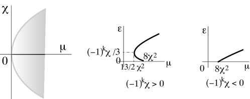
Figure 3: Domain of existence (shaded) of bifurcating unequal amplitude QP-super-hexagons, for small $|\chi|$. These solutions only bifurcate from $\mu=0$ when $\chi=0$.

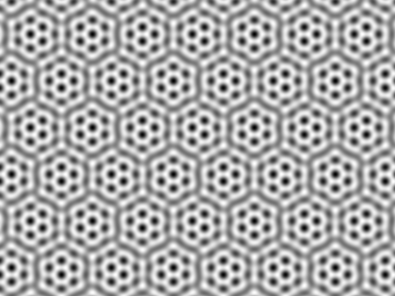
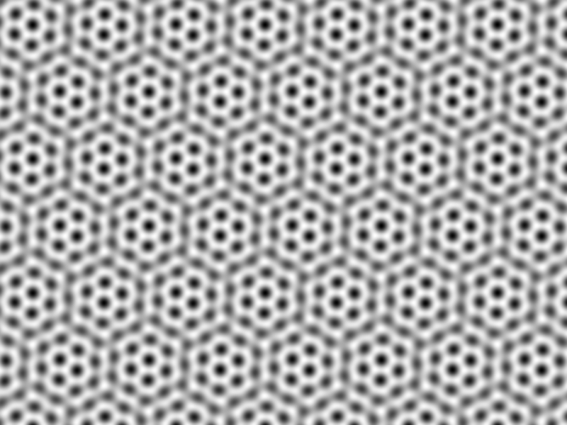
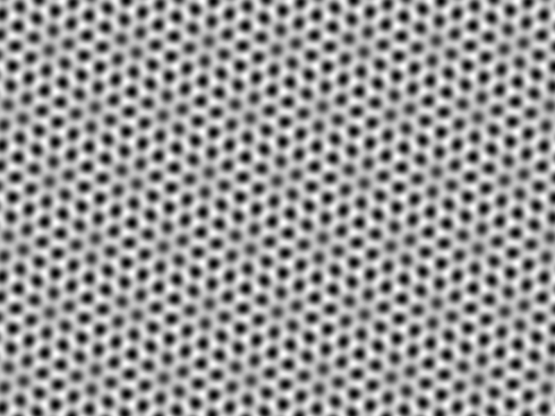
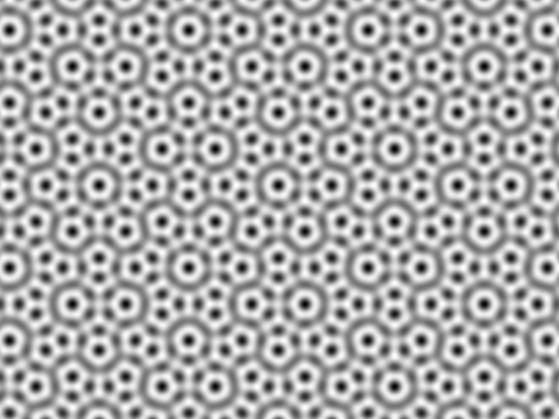
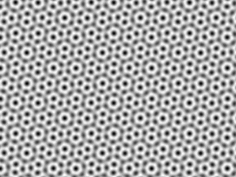
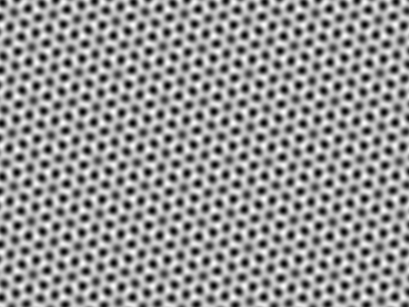
Figure 4: Examples of quasipatterns: superposition of hexagons. Top row: $\alpha=\frac{\pi}{12}=15^{\circ}$; bottom row: $\alpha=25.66^{\circ}$ ($\cos\alpha=\frac{1}{4}\sqrt{13}$). Left: equal amplitude QP-super-hexagons; center and right: unequal amplitude QP-super-hexagons, with $k=k^{\prime}$ (center) and $k=k^{\prime}+1$ (right).

Theorem 4.2 (Quasiperiodic superposed hexagons).

Assume $\alpha\in{\mathcal{E}_{0}}\cap{\mathcal{E}_{qp}}$, then for $\varepsilon,\chi$ fixed, we can build a four-parameter formal power series solution of Eq. 14 of the form

(30) $$u(\varepsilon,\chi,k,\Theta) =\varepsilon u_{1}+\sum_{n\geq 2}\varepsilon^{n}u_{n}(\chi,k,\Theta),\quad\varepsilon>0,\quad u_{n}\bot e^{i{\mathbf{k}}_{j}\cdot{\mathbf{x}}},\quad j=1,\dots,6,$$

$$\mu(\varepsilon,\chi,k) =(-1)^{k}2\chi\varepsilon+\mu_{2}(\chi)\varepsilon^{2}+\sum_{n\geq 3}\varepsilon^{n}\mu_{n}(\chi,k),\text{ }k=0,1,$$

$$\text{with}\quad u_{1} =\sum_{j=1,\dots,6}e^{i({\mathbf{k}}_{j}\cdot{\mathbf{x}}+\theta_{j})}+c.c.,\quad\Theta=(\theta_{1},\dots,\theta_{6}),$$

$$\mu_{2}(\chi) =33-\chi^{2}(c_{1}+2c_{2}+c_{\alpha}+c_{\alpha+}+c_{\alpha-})$$

$$\theta_{1}+\theta_{2}+\theta_{3} =k\pi,\quad\theta_{4}+\theta_{5}+\theta_{6}=k^{\prime}\pi,\quad k=k^{\prime}=0,1$$

$$u_{n}(-\chi,k,\Theta) =(-1)^{n+1}u_{n}(\chi,k,\Theta),\quad\mu_{n}(-\chi,k)=(-1)^{n}\mu_{n}(\chi,k).$$

These are the equal amplitude QP-super-hexagons. Moreover, for a range of $(\mu,\chi)$ close to 0 (see Fig. 3), there are in addition two unequal amplitude QP-super-hexagon solutions (for $k=0,1$), given by

$$u(\varepsilon,\chi,k,\Theta) =\varepsilon u_{10}+\delta u_{11}+\sum_{m+p\geq 2}\varepsilon^{m}\chi^{p}u_{mp}(k,\Theta),\quad\varepsilon>0,\delta>0,$$

$$\quad u_{mp}\bot e^{i{\mathbf{k}}_{j}\cdot{\mathbf{x}}},\quad j=1,\dots,6,\quad u\text{ odd in }(\varepsilon,\chi),$$

(31) $$u_{10} =\sum_{j=1,2,3}e^{i({\mathbf{k}}_{j}\cdot{\mathbf{x}}+\theta_{j})}+c.c.,\quad u_{11}=\sum_{j=4,5,6}e^{i({\mathbf{k}}_{j}\cdot{\mathbf{x}}+\theta_{j})}+c.c.,$$

$$\theta_{1}+\theta_{2}+\theta_{3} =k\pi,\quad k=0,1,\quad\theta_{4}+\theta_{5}+\theta_{6}=k^{\prime}\pi,\quad k^{\prime}=0,1\text{\ determined below},$$

$$\delta(\varepsilon,\chi,k) =(-1)^{k^{\prime}}\left\{\frac{2\chi}{3}-(-1)^{k}\varepsilon+\sum_{m+p\geq 2}\varepsilon^{m}\chi^{p}\delta_{mp}(k)\right\},\quad(-1)^{k^{\prime}}\delta\text{ odd in }((-1)^{k}\varepsilon,\chi),$$

$$\mu(\varepsilon,\chi,k) =33\varepsilon^{2}-22(-1)^{k}\varepsilon\chi+8\chi^{2}+\sum_{m+p\geq 3}\varepsilon^{m}\chi^{p}\mu_{mp}(k),\quad\mu\text{ even in }((-1)^{k}\varepsilon,\chi).$$

In the expression for $\delta$, $k^{\prime}$ is chosen so that $\delta>0$. For either type of solution, changing $\theta_{1},\theta_{2},\theta_{4},\theta_{5}$ corresponds to translating each hexagonal pattern arbitrarily. Figure 4 shows examples of $u_{1}$ for the two types of superposed hexagon quasipatterns, for two values of $\alpha$.

Then, for $\alpha\in{\mathcal{E}_{2}}$, which is included in ${\mathcal{E}_{0}}\cap{\mathcal{E}_{qp}}$, and using the same proof as in [25], both types of bifurcating quasipattern solutions of Eq. 1 are proved to exist. The equal amplitude QP-super-hexagons have asymptotic expansion Eq. 30, provided that $\varepsilon$ is small enough, and the unequal amplitude QP-super-hexagons have asymptotic expansion Eq. 31, provided that $\varepsilon,\chi$ are small enough.

Remark 4.3.

Symmetries of quasipatterns are hard to write down precisely [7] since the arbitrary relative position of the two hexagonal patterns may mean that there is no point of rotation symmetry or line of reflection symmetry. Nonetheless, with $\varepsilon=\delta$, the first type of solution is symmetric ‘on average’ under rotations by $\frac{\pi}{3}$ and reflections conjugate to $\mathbf{\tau}$. In fact the 4 parameter family of solutions is globally invariant under symmetries $\mathbf{R}_{\pi/3}$ and $\mathbf{\tau}$. Notice that, for the unequal amplitude QP-super-hexagon solutions, the reflection symmetry $\mathbf{\tau}$ exchanges $(k,\varepsilon)$ with $(k^{\prime},\delta)$.

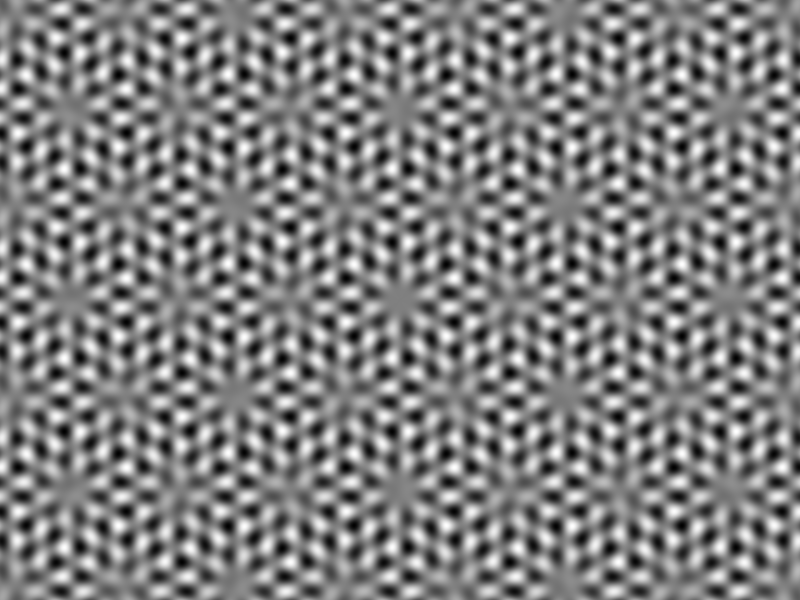
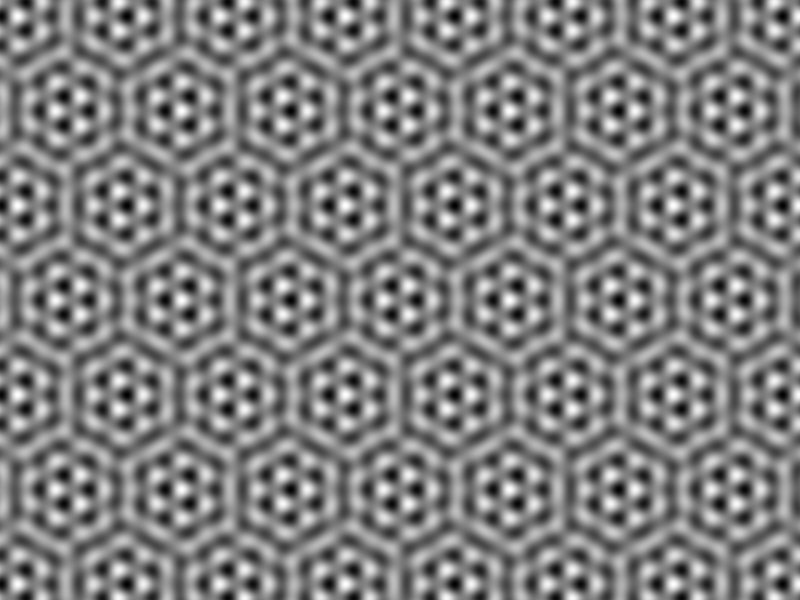
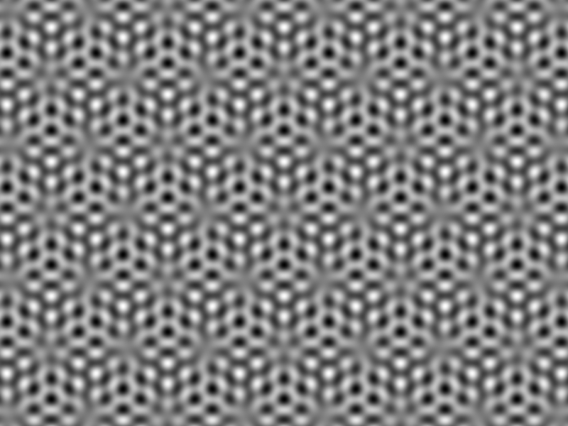
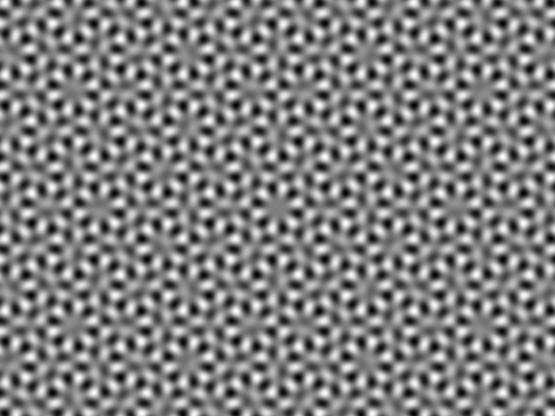
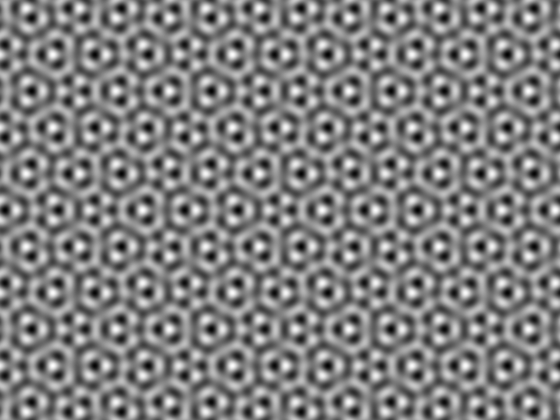
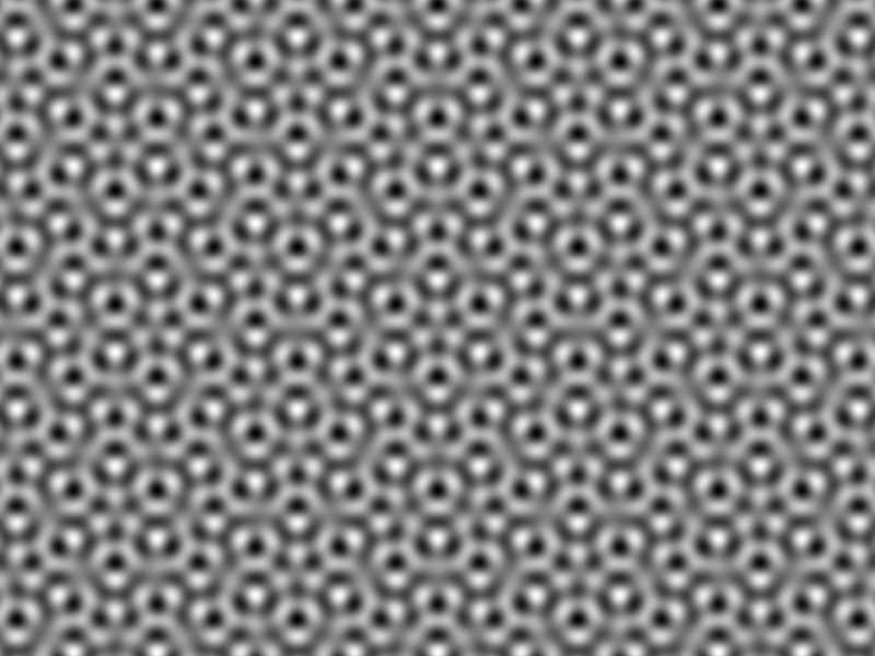
Figure 5: Examples of quasipatterns: superposition of hexagons with $\chi=0$. Top row: $\alpha=\frac{\pi}{12}=15^{\circ}$; bottom row: $\alpha=25.66^{\circ}$ ($\cos\alpha=\frac{1}{4}\sqrt{13}$). Left: QP-anti-hexagons; center: QP-super-triangles; right: QP-anti-triangles.

Remark 4.4.

Let us observe that equal amplitude QP-super-hexagons for $\theta_{j}=0$, $j=1,\dots,6$ were already obtained for $\chi=0$ in [25].

In the case $\chi=0$, the unequal amplitude solutions do not exist. The original system Eq. 1 is equivariant under the symmetry $\mathbf{S}$, which implies that in Eq. 18, $f_{1}$ and $f_{2}$ are respectively even and odd in $(q_{1},q_{4})$. For $\varepsilon=\delta$ the bifurcation system reduces to two equations of the form

$$\mu = f_{1}(\mu,\varepsilon^{2},q_{1},q_{4})+\varepsilon e^{-i\Theta_{1}}f_{2}(\mu,\varepsilon^{2},q_{1},q_{4})$$

$$\mu = f_{1}(\mu,\varepsilon^{2},q_{4},q_{1})+\varepsilon e^{-i\Theta_{4}}f_{2}(\mu,\varepsilon^{2},q_{4},q_{1}),$$

and we may observe new quasipattern solutions, illustrated in Fig. 5. The names here are analagous to the related periodic patterns [15].

QP-anti-hexagons are obtained for (also obtained in [25])

$$\theta_{j} = 0,\qquad j=1,2,3,$$

$$\theta_{j} = \pi,\qquad j=4,5,6,$$

which leads to

$$e^{-i\Theta_{1}} = 1,\text{ }e^{-i\Theta_{4}}=-1,$$

$$q_{1} = \varepsilon^{3}=-q_{4},$$

and the parity properties of $f_{j}$ give only one bifurcation equation

$$\mu=f_{1}(\mu,\varepsilon^{2},\varepsilon^{3},-\varepsilon^{3})+\varepsilon f_{2}(\mu,\varepsilon^{2},\varepsilon^{3},-\varepsilon^{3}).$$

QP-super-triangles are obtained for

$$\theta_{j}=\pi/2,\qquad j=1,\dots,6,$$

which leads to

$$e^{-i\Theta_{1}} = e^{-i\Theta_{4}}=i,$$

$$q_{1} = -i\varepsilon^{3}=q_{4},$$

and it is clear that we have only one real bifurcation equation, with evenness (resp. oddness) with respect to the two last arguments of $f_{1}$ (resp. $f_{2}$) leading to

$$\mu=f_{1}(\mu,\varepsilon^{2},-i\varepsilon^{3},-i\varepsilon^{3})+i\varepsilon f_{2}(\mu,\varepsilon^{2},-i\varepsilon^{3},-i\varepsilon^{3}).$$

QP-anti-triangles are obtained for

$$\theta_{j} = \pi/2\qquad j=1,2,3,$$

$$\theta_{j} = -\pi/2,\qquad j=4,5,6,$$

which leads to

$$e^{-i\Theta_{1}} = i,\text{ }e^{-i\Theta_{4}}=-i,$$

$$q_{1} = -i\varepsilon^{3}=-q_{4},$$

and the parity properties of $f_{j}$ give only one real bifurcation equation

$$\mu=f_{1}(\mu,\varepsilon^{2},-i\varepsilon^{3},i\varepsilon^{3})+i\varepsilon f_{2}(\mu,\varepsilon^{2},-i\varepsilon^{3},i\varepsilon^{3}).$$

All these cases lead to series for $u$ and $\mu$, respectively odd and even in $\varepsilon$, and hence quasiperiodic anti-hexagons, super-triangles and anti-triangles in Eq. 1 for $\alpha\in{\mathcal{E}_{2}}$ and for $\chi=0$. Using the same arguments as above, we can say that these QP-anti-hexagons etc. are solutions of the PDE with $\chi=0$.

4.2.2 Periodic case: Higher orders

In this case we have more resonant terms in the bifurcation equation, as seen in Eq. 19. These resonant terms introduce relations between the phases of the complex amplitudes, so the periodic superposed hexagon solutions come in two-parameter, rather than four-parameter, families. We consider here only the equal amplitude solutions, with $\varepsilon=\delta$, but even in this case there are two sub-types of solutions: super-hexagon solutions, and triangular superlattice solutions, where the phase relationships depend on amplitude. The triangular superlattice solutions we find are generalizations of those found by [45]; the name comes from the triagular appearance of the $(a,b)=(3,2)$ version of this periodic pattern (see Fig. 1a and [29]).

Super-hexagons

We notice that, in setting

$$z_{j}=\varepsilon e^{i\theta_{j}},\quad\varepsilon>0,\quad j=1,\dots,6$$

and taking

(32) $$\theta_{1}=\theta_{2}=\theta_{3}=-\theta_{4}=-\theta_{5}=-\theta_{6}=k\frac{\pi}{3}$$

we have  $q_{1}=q_{4}=(-1)^{k}\varepsilon^{3}$ and we can check that the nine sets $G_{j}$ of invariant monomials satisfy (see Appendix D)

$$G_{1} =\varepsilon^{2a}, G_{2} =G^{\prime}_{2}=\varepsilon^{3a-b}e^{i(a+b)k\pi}, G_{3} =G^{\prime}_{3}=\varepsilon^{2a+b}e^{ibk\pi},$$

$$G_{4} =\varepsilon^{4a-2b}, G_{5} =G^{\prime}_{5}=\varepsilon^{3a}e^{iak\pi}, G_{6} =\varepsilon^{2a+2b},$$

all these monomials being real. In Appendix D we show that each group on the same line above is invariant under the actions of $\mathbf{R}_{\pi/3}$ and $\mathbf{\tau}$. It then follows that the system of bifurcation equations reduces to only one equation with real coefficients, as in the quasiperiodic case for the first solutions. We have now a solution of the form

$$z_{1} = z_{2}=z_{3}=\varepsilon e^{i\theta},$$

$$z_{4} = z_{5}=z_{6}=\varepsilon e^{-i\theta},\text{ }\theta=k\frac{\pi}{3},\text{ \ }k=0,\dots,5.$$

The conclusion is that the power series starting as in Eq. 25 for $\mu$ in terms of $\varepsilon$ is still valid for the periodic case (the modifications occuring at high order), provided we restrict the choice of arguments $\theta_{j}$ as Eq. 32. We show in Appendix F that solutions with $k=0,2,4$ or with $k=1,3,5$ may be obtained from one of them, in acting a suitable translation $\mathbf{T}_{\mathbf{\delta}}$. It follows that we only find two different bifurcating patterns, corresponding to opposite signs of $\mu$. Moreover, we notice that the solution obtained for $k=0$ is changed into the solution obtained for $k=3$ by acting the symmetry $\mathbf{S}$ on it, and changing $\chi$ into $-\chi$. Finally, notice that since the Lyapunov–Schmidt method applies in this case, the series converges, for $\varepsilon$ small enough. The above solutions have arguments $\theta_{j}=0$ or $\pi$ that do not depend on parameters $(\mu,\chi)$; these solutions correspond to super-hexagons.

Triangular superlattice solutions

Now, in [45] other solutions were found for $(a,b)=(3,2)$, just taking into account of terms of order five in the bifurcation system. Let us show that these solutions exist indeed for any $(a,b)$ and taking into account of all resonant terms.

Let us consider the particular cases with

$$z_{j}=\varepsilon e^{i\theta},$$

then the nine sets $G_{j}$ of monomials defined in Appendix D satisfy

$$G_{1} = \varepsilon^{2a}e^{i(4b-2a)\theta},\text{ }\mathbf{R}_{\pi/3}G_{1}=\overline{G_{1}},\text{ }\tau G_{1}=G_{1},$$

$$G_{2} = G_{2}^{\prime}=\varepsilon^{3a-b}e^{i(a+b)\theta},\text{ }\mathbf{R}_{\pi/3}G_{2}=\overline{G_{2}},\text{ }\tau G_{2}=G_{2},$$

$$G_{3} = \overline{G_{3}^{\prime}}=\varepsilon^{2a+b}e^{i(2a-b)\theta},\text{ }\mathbf{R}_{\pi/3}G_{3}=\overline{G_{3}},\text{ }\tau G_{3}=G_{3},$$

$$G_{4} = \varepsilon^{4a-2b}e^{i(4a-2b)\theta},\text{ }\mathbf{R}_{\pi/3}G_{4}=\overline{G_{4}},\text{ }\tau G_{4}=G_{4},$$

$$G_{5} = \overline{G_{5}^{\prime}}=\varepsilon^{3a}e^{i(2b-a)\theta},\text{ \ }\mathbf{R}_{\pi/3}G_{5}=\overline{G_{5}},\text{ }\tau G_{5}=G_{5},$$

$$G_{6} = \varepsilon^{2a+2b}e^{i(2a+2b)\theta},\text{ \ }\mathbf{R}_{\pi/3}G_{6}=\overline{G_{6}},\text{ }\tau G_{6}=G_{6}.$$

Then the first bifurcation equation becomes

(33) $$\mu=f_{3}+\varepsilon e^{-3i\theta}f_{4}+\frac{G_{1}}{\varepsilon^{2}}f_{G_{1}}+\frac{G_{2}}{\varepsilon^{2}}f_{G_{2}}+\frac{\overline{G_{4}}}{\varepsilon^{2}}f_{G_{4}}+\frac{\overline{G_{5}}}{\varepsilon^{2}}f_{G_{5}}+\frac{\overline{G_{6}}}{\varepsilon^{2}}f_{G_{6}},$$

with all $f_{j}$ functions of $(\chi,\mu,\varepsilon^{2},\varepsilon^{3}e^{3i\theta},\varepsilon^{3}e^{-3i\theta},G_{1},\overline{G_{1}},G_{2},\overline{G_{2}},G_{3},\overline{G_{3}},G_{4},\overline{G_{4}},G_{5},\overline{G_{5}},G_{6},\overline{G_{6}})$. They have real coefficients, and are invariant under symmetry $\mathbf{\tau}$, while the arguments are changed into their complex conjugate by symmetry $\mathbf{R}_{\pi/3}$. It follows that the bifurcation system reduces to only one complex (because of the occurrence of $\theta$) equation, where we can express the unknowns $(\mu,\theta)$ as functions of $\varepsilon$. Then truncated at cubic order in $(\mu,\varepsilon)$ this equation reads

$$\mu=f_{3}^{(0)}(\chi,\varepsilon^{2},\varepsilon^{3}e^{3i\theta},\varepsilon^{3}e^{-3i\theta})+\varepsilon e^{-3i\theta}f_{4}^{(0)}(\chi,\varepsilon^{2}),$$

which is a nice perturbation at order $\varepsilon^{3}$ of the known equation

$$\mu=(\alpha_{1}+2\alpha_{2}+\alpha_{4}+\alpha_{5}+\alpha_{6})\varepsilon^{2}+2\chi\varepsilon e^{-3i\theta}.$$

This leads to the two types of solutions:

$$e^{3i\theta} = \pm 1,$$

$$\mu = f_{3}^{(0)}(\chi,\varepsilon^{2},\pm\varepsilon^{3},\pm\varepsilon^{3})\pm\varepsilon f_{4}^{(0)}(\chi,\varepsilon^{2}).$$

These solutions are not degenerate, so that, if we consider the complex equation Eq. 33, the implicit function theorem applies for solving with respect to $(\mu,\theta)$ in convergent powers series of $\varepsilon$. This gives solutions of the form

$$\theta_{l}(\varepsilon) = l\frac{\pi}{3}+\mathcal{O}(\varepsilon),\text{ }l=0,1,2,3,4,5$$

$$\mu = f_{3}^{(0)}(\chi,\varepsilon^{2},(-1)^{l}\varepsilon^{3},(-1)^{l}\varepsilon^{3})+(-1)^{l}\varepsilon f_{4}^{(0)}(\chi,\varepsilon^{2})+\mathcal{O}(\varepsilon^{4}).$$

Now, we observe that the cases $l=0,3$ lead to a real bifurcation equation, which fixes the argument $\theta=0$ or $\pi$. This recovers the super-hexagon solutions, already found. The remaining cases are the solutions suggested by [45] (for $(a,b)=(3,2)$, not including all resonant terms). Let us sum up the results in the following

Theorem 4.5 (Periodic equal amplitude superposed hexagons).

Assume $\alpha\in{\mathcal{E}_{0}}\cap{\mathcal{E}_{p}}$, then for $\varepsilon$ small enough, and $\chi$ fixed, we can build convergent power series solutions of Eq. 14, of the form

$$u(\varepsilon,\chi,k) =\varepsilon u_{1}+\sum_{n\geq 2}\varepsilon^{n}u_{n}(\chi,k),\text{ \ }u_{n}\bot e^{i{\mathbf{k}}_{j}\cdot{\mathbf{x}}},\text{ \ }j=1,\dots,6,\text{ \ }n\geq 2$$

(34) $$\mu(\varepsilon,\chi,k) =(-1)^{k}2\chi\varepsilon+\mu_{2}(\chi)\varepsilon^{2}+\sum_{n\geq 3}\varepsilon^{n}\mu_{n}(\chi,k),$$

$$u_{n}(-\chi,k) =(-1)^{n}u_{n}(\chi,k),\text{ \ }\mu_{n}(-\chi,k)=(-1)^{n}\mu_{n}(\chi,k);$$

where $\mu$ is even in $((-1)^{k}\varepsilon,\chi)$ and $\mu_{2}(\chi)$ is defined at Theorem 4.2 and such that, for super-hexagon solutions

$$u_{1}=\sum_{j=1,\dots,6}e^{i({\mathbf{k}}_{j}\cdot{\mathbf{x}}+\theta_{j})}+c.c.,\text{ }\theta_{1}=\theta_{2}=\theta_{3}=-\theta_{4}=-\theta_{5}=-\theta_{6}=k\pi,\text{ }k=0,\text{ or }1.$$

For triangular superlattice solutions, we have

$$u_{1}=\sum_{j=1,\dots,6}e^{i({\mathbf{k}}_{j}\cdot{\mathbf{x}}+\theta)}+c.c.,\text{ }\theta(\varepsilon,\chi,k)=k\frac{\pi}{3}+\sum_{n\geq 1}\varepsilon^{n}\theta_{n}(\chi,k),,k=1,2,4,5.$$

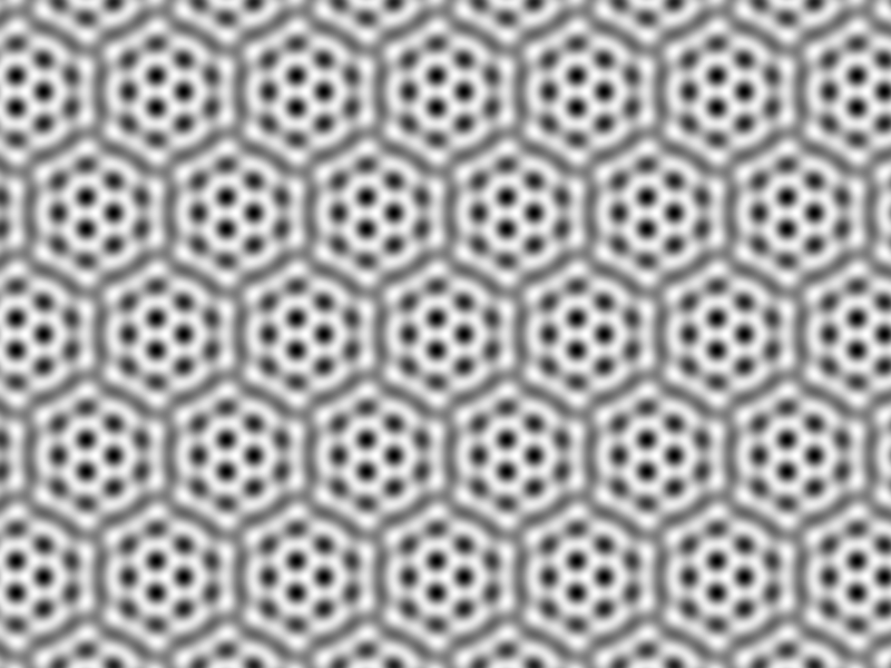
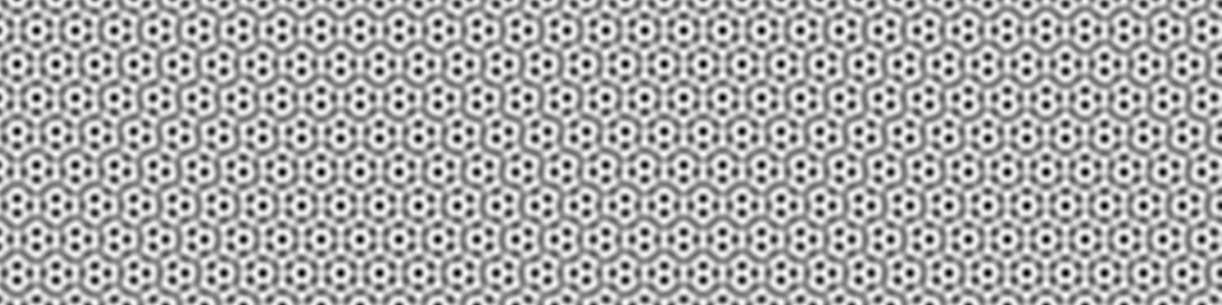
Figure 6: Examples of periodic patterns: superposition of hexagons. Top row: $\alpha=13.17^{\circ}$ ($\cos\alpha=\frac{37}{38}$, $(a,b)=(5,3)$); middle row: $\alpha=21.79^{\circ}$ ($\cos\alpha=\frac{13}{14}$, $(a,b)=(3,2)$ – see also Fig. 1a). For these, the left column (super-hexagons) has $\theta_{j}=0$ for $j=1,\dots,6$. The middle and right (superlattice triangles) have $\theta_{j}=\frac{2\pi}{3}$ and $\theta_{j}=\frac{4\pi}{3}$ respectively. The bottom row shows a related quasiperiodic example with $\alpha=21.00^{\circ}$, close to $21.79^{\circ}$, showing long-range modulation between the three periodic patterns in the middle row.

Remark 4.6.

For triangular superlattice solutions, the phases of the amplitudes are not independent of the parameters, in contrast to the super-hexagon solutions. These patterns are illustrated in Fig. 6. The figure includes (middle row) periodic patterns with $\alpha=21.79^{\circ}$ and (bottom row) a quasiperiodic pattern with $\alpha=21^{\circ}$, showing how, with a slightly different value of $\alpha$, the quasiperiodic pattern modulates between the three periodic solutions with $l=0,2,4$.

Remark 4.7.

In the $\chi=0$ case, we can recover all the solutions found by [15] using these ideas.

4.3 Hexa-rolls: superposition of hexagons and rolls

As in §4.2, we start with the cubic truncation of the quasiperiodic and periodic cases together, then consider the effect of higher order terms. Here we consider the case where $q_{1}\neq 0$ and $q_{4}=0$ in Eq. 20, so that we assume now

$$q_{1}\neq 0,\text{ \ }z_{4}\neq 0,\text{ \ }z_{5}=z_{6}=0.$$

Then the system Eq. 20 reduces to 4 equations

$$2\chi\overline{q_{1}} =u_{1}[\mu-\alpha_{1}u_{1}-\alpha_{2}(u_{2}+u_{3})-\alpha_{4}u_{4}],$$

$$2\chi\overline{q_{1}} =u_{2}[\mu-\alpha_{1}u_{2}-\alpha_{2}(u_{1}+u_{3})-\alpha_{6}u_{4}],$$

(35) $$2\chi\overline{q_{1}} =u_{3}[\mu-\alpha_{1}u_{3}-\alpha_{2}(u_{1}+u_{2})-\alpha_{5}u_{4}],$$

$$0 =\mu-\alpha_{1}u_{4}-\alpha_{4}u_{1}-\alpha_{5}u_{3}-\alpha_{6}u_{2},$$

where again this implies that $q_{1}$ is real. Below, we study solutions of the bifurcation problem, built on a lattice spanned by the four wave vectors ${\mathbf{k}}_{1}$, ${\mathbf{k}}_{2}$, ${\mathbf{k}}_{3}$, and ${\mathbf{k}}_{4}$, and so we find solutions composed of a superposition of hexagons and rolls. Unlike in the super-hexagon cases above, the three amplitudes ($|z_{1}|$, $|z_{2}|$ and $|z_{3}|$) of the hexagonal part of the pattern are of similar size but will not be exactly equal. We find two different types of solution distinguished by the relative magnitudes of the hexaonal and roll parts of the pattern. The first type occurs when $|\chi|$ is neither too small nor too large and is such that rolls dominate the hexagons. The second type occurs only for small $|\chi|$ and is such that rolls and hexagons are more balanced.

4.3.1 Hexa-rolls: rolls dominate hexagons

A consistent balance of terms in Eq. 35 is to have $u_{1}$, $u_{2}$ and $u_{3}$ be $\mathcal{O}(\mu^{2})$, so that $q_{1}$ is $\mathcal{O}(\mu^{3})$, while $u_{4}$ is $\mathcal{O}(\mu)$. With this balance, at leading order we have the reduced system

$$2\chi\overline{q_{1}} =u_{1}[\mu-\alpha_{4}u_{4}],$$

(36) $$2\chi\overline{q_{1}} =u_{2}[\mu-\alpha_{6}u_{4}],$$

$$2\chi\overline{q_{1}} =u_{3}[\mu-\alpha_{5}u_{4}],$$

$$0 =\mu-\alpha_{1}u_{4},$$

which leads to

$$z_{j} = \sqrt{u_{j}}e^{i\theta_{j}},\quad j=1,2,3,$$

$$u_{j} = \mu^{2}u_{j}^{(0)},\quad u_{4}=\frac{\mu}{\alpha_{1}},$$

$$\Theta_{1} = \theta_{1}+\theta_{2}+\theta_{3}=k\pi,$$

with

$$u_{1}^{(0)} =\frac{(\alpha_{5}-\alpha_{1})(\alpha_{6}-\alpha_{1})}{4\chi^{2}\alpha_{1}^{2}},$$

(37) $$u_{2}^{(0)} =\frac{(\alpha_{5}-\alpha_{1})(\alpha_{4}-\alpha_{1})}{4\chi^{2}\alpha_{1}^{2}},$$

$$u_{3}^{(0)} =\frac{(\alpha_{4}-\alpha_{1})(\alpha_{6}-\alpha_{1})}{4\chi^{2}\alpha_{1}^{2}},$$

$$(-1)^{k} =\text{sign}[\chi(\alpha_{1}-\alpha_{4})].$$

The condition for the existence of this solution is that $(\alpha_{4}-\alpha_{1})$, $(\alpha_{5}-\alpha_{1})$, $(\alpha_{6}-\alpha_{1})$ should be nonzero and have the same sign. This condition is realized in Eq. 1 provided that

$$3+\chi^{2}(c_{1}-c_{\alpha}),\qquad 3+\chi^{2}(c_{1}-c_{\alpha+}),\qquad 3+\chi^{2}(c_{1}-c_{\alpha-}),$$

have the same sign, which holds at least for $|\chi|$ not too large. For applying later the implicit function theorem, we typically need $|\mu|\ll\min(1,|\chi|)$, so $|\chi|$ should also be not too small. Here, for $|\chi|$ not too large, $\alpha_{1}>0$, so the bifurcation is supercritical in this case.

Now let us consider the full bifurcation system. Setting

(38) $$u_{j}=\mu^{2}u_{j}^{(0)}(1+x_{j}),\quad j=1,2,3,\quad u_{4}=\frac{\mu}{a_{1}}(1+x_{4}),$$

we replace these expressions in Eq. 35 plus higher order terms appearing in Eq. 18 or Eq. 19, and noticing that we obtain a real system of four equations in all periodic and quasiperiodic cases except in the periodic case when $a-b=1$, as defined in Lemma 2.2.

Remark 4.8.

In the case $\alpha=\frac{\pi}{6}$, this combination of hexagons and rolls was reported by [32, 28, 49].

Remark 4.9.

In the periodic case when $a-b=1$, a careful examination of high order resonant terms (as defined in Appendix D) shows that there remains six equations, instead of four. We might compute some new solution looking like the superposed hexagons and rolls (but with small $|z_{5}|$ and $|z_{6}|$), however there are not strictly of the required form since $q_{1}q_{4}\neq 0$. We do not pursue these solutions further here.

Then, dividing the first three equations in Eq. 36 (with Eq. 38) by $\mu^{3}$, dividing the fourth one by $\mu$, and computing the linear part in $x_{j}$, we obtain

$$a(x_{1}+x_{2}+x_{3})-u_{1}^{(0)}((1-\frac{\alpha_{4}}{\alpha_{1}})x_{1}-\frac{\alpha_{4}}{\alpha_{1}}x_{4}) =h_{1},$$

(39) $$a(x_{1}+x_{2}+x_{3})-u_{2}^{(0)}((1-\frac{\alpha_{6}}{\alpha_{1}})x_{2}-\frac{\alpha_{6}}{\alpha_{1}}x_{4}) =h_{2},$$

$$a(x_{1}+x_{2}+x_{3})-u_{3}^{(0)}((1-\frac{\alpha_{5}}{\alpha_{1}})x_{3}-\frac{\alpha_{5}}{\alpha_{1}}x_{4}) =h_{3},$$

$$x_{4} =h_{4},$$

with

$$a=(-1)^{k}\chi\sqrt{u_{1}^{(0)}u_{2}^{(0)}u_{3}^{(0)}},$$

and all $h_{j}$ have $\mu$ in factor. The left hand side of the system Eq. 39 represents the differential at the origin with respect to $(x_{1},x_{2},x_{3},x_{4})$, defining a matrix $M^{\prime}$ that needs to be inverted in order to use the implicit function theorem. The determinant of matrix $M^{\prime}$ can be computed and it is

$$\frac{[3(-1)^{k}\text{sign}(\chi)-2]}{128\chi^{6}\alpha_{1}^{9}}[(\alpha_{1}-\alpha_{4})(\alpha_{1}-\alpha_{5})(\alpha_{1}-\alpha_{6})]^{3},$$

which is not zero. Therefore the implicit function theorem applies, so we can find series in powers of $\mu$ for $(x_{1},x_{2},x_{3},x_{4})$ solving the full bifurcation system in both the quasiperiodic case Eq. 18 and the periodic case Eq. 19. We can state the following

Theorem 4.10 (Hexa-rolls: superposed hexagons and rolls with rolls dominant).

Assume that $\alpha\in{\mathcal{E}_{0}}$, and in case of a periodic lattice assume $a-b>1$. Then for fixed values of $\chi$ such that

$$(\alpha_{4}-\alpha_{1}),(\alpha_{5}-\alpha_{1}),(\alpha_{6}-\alpha_{1})$$

are nonzero and have the same sign, and for $\mu$ close enough to $0$, we can build a three-parameter formal power series in $\varepsilon$ solution of Eq. 1 of the form

$$u(\varepsilon,\Theta,\chi,j) = u_{1}(\varepsilon,\Theta,\chi,j)+\sum\limits_{n\geq 3}\varepsilon^{n}u_{n}(\chi,\Theta,j),\quad u_{2p+1}\bot e^{i{\mathbf{k}}_{j}\cdot{\mathbf{x}}},\quad j=4,\text{ or }5\text{ or }6,$$

$$u_{1}(\varepsilon,\Theta,\chi,j) = \varepsilon e^{i({\mathbf{k}}_{j}\cdot\mathbf{x}+\theta_{j})}+\alpha_{1}\varepsilon^{2}\sum_{m=1,2,3}\sqrt{u_{m}^{(0)}}e^{i({\mathbf{k}}_{m}\cdot\mathbf{x}+\theta_{m})}+c.c.$$

$$\Theta = (\theta_{1},\theta_{2},\theta_{3},\theta_{j}),\text{ \ }\theta_{1}+\theta_{2}+\theta_{3}=k\pi,\text{ }k=0\text{ or }1,$$

$$\mu(\varepsilon,\chi,j) = \alpha_{1}\varepsilon^{2}+\sum_{n\geq 2}\mu_{2n}(\chi,j)\varepsilon^{2n},\text{ even in }\varepsilon,$$

where $u_{m}^{(0)}$ and $k$ are determined in Eq. 37. For $\alpha_{1}>0$ the bifurcation is supercritical with $\mu>0$. In the case $\alpha_{1}<0$, subcritical patterns can be found with $\mu<0$. In the quasiperiodic case ($\alpha\in{\mathcal{E}_{2}}$), these solutions give quasipatterns using the techniques of [25]. In the periodic case ($\alpha\in{\mathcal{E}_{p}}\cap{\mathcal{E}_{0}}$), the classical Lyapunov–Schmidt method give periodic pattern solutions of the PDE Eq. 1. In both cases, the freedom left for $\Theta$ corresponds to an arbitrary choice for translations $\mathbf{T}_{\delta}$ of the hexagons, and the arbitrary choice of $\theta_{j}$ ($j=4,5,6$) allows an arbitrary relative translation of the rolls. Figure 7 shows quasiperiodic examples of $u_{1}$ (QP-hexa-rolls).

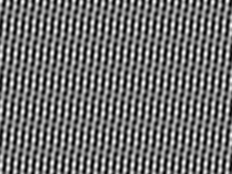
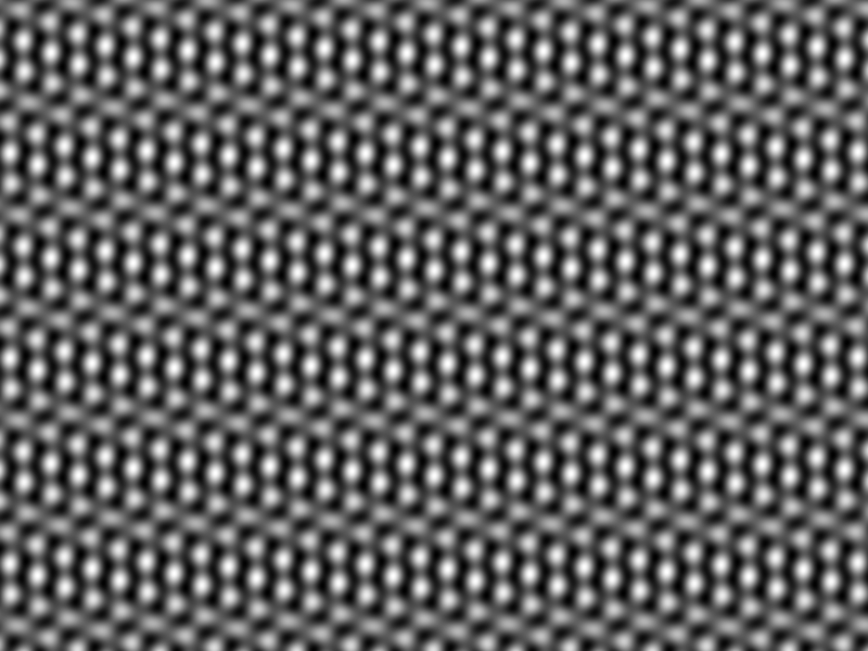
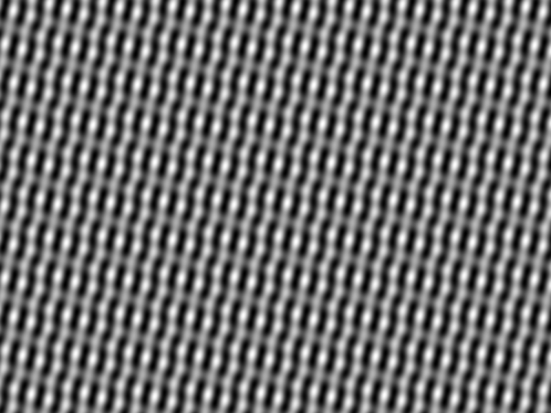
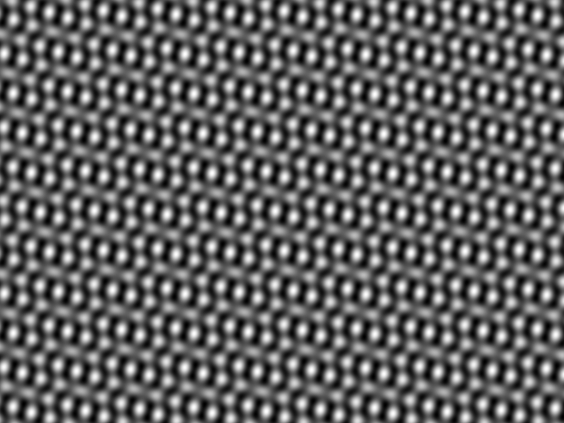
Figure 7: Examples of quasipatterns: superposition of hexagons and rolls. Top row: $\alpha=\frac{\pi}{12}=15^{\circ}$; bottom row: $\alpha=25.66^{\circ}$ ($\cos\alpha=\frac{1}{4}\sqrt{13}$). Left: QP-hexa-rolls with rolls dominating hexagons; right: QP-hexa-rolls with rolls and hexagons in balance.

Remark 4.11.

These hexa-roll solutions are new, even in the case of a periodic lattice. They have the surprising feature in the periodic case of allowing arbitrary relative translations between the hexagons and rolls. Unlike the super-hexagon solutions, these solutions require a condition on the cubic coefficients to be satisfied in order to exist. They were not found by [15] since there the equivariant branching lemma was used, which finds only solutions that are characterized by a single amplitude (these solutions have two) and that exist for all non-degenerate values of the cubic coefficients (here the cubic coefficients must satisfy an inequality).

4.3.2 Hexa-rolls: rolls and hexagons balance

With small $|\chi|$, solutions can be found where the rolls and hexagons are of similar size. Let us consider the system Eq. 35, without the terms with $\chi^{2}$ in coefficients, and set

$$z_{1} =\varepsilon e^{i\theta_{1}},\qquad z_{2}=\varepsilon e^{i\theta_{2}}, z_{3} =\varepsilon\zeta_{3}e^{i\theta_{3}}, \theta_{1} +\theta_{2}+\theta_{3}=k\pi, \varepsilon >0,$$

$$u_{4} =|z_{4}|^{2}=\varepsilon^{2}u_{4}^{(0)}, z_{5} =z_{6}=0, \mu =\varepsilon^{2}\mu^{(0)}, \chi =\varepsilon\kappa,$$

then, after division by $\varepsilon^{4}$ the first equations, and by $\varepsilon^{2}$ the fourth one, this gives

$$2\kappa(-1)^{k}\zeta_{3} = \mu^{(0)}-9-6\zeta_{3}^{2}-6u_{4}^{(0)},$$

$$2\kappa(-1)^{k}\zeta_{3} = \zeta_{3}^{2}[\mu^{(0)}-3\zeta_{3}^{2}-12-6u_{4}^{(0)})],$$

$$0 = \mu^{(0)}-3u_{4}^{(0)}-12-6\zeta_{3}^{2}.$$

Eliminating $\mu^{(0)}$ and $u_{4}^{(0)}$ leads to

$$u_{4}^{(0)}=1-\frac{2\kappa}{3}\zeta_{3}(-1)^{k},$$

and

$$(3\zeta_{3}+2\kappa(-1)^{k})(\zeta_{3}^{2}-1)=0.$$

Balanced hexa-rolls type 1

For the solution $\zeta_{3}=1$, we obtain

(40) $$z_{3}=\varepsilon e^{i\theta_{3}},\text{ }u_{4}^{(0)}=1+\frac{2\kappa}{3}(-1)^{k+1},\text{ }\mu^{(0)}=21+2\kappa(-1)^{k+1},$$

for which we need to satisfy $u_{4}^{(0)}>0$, i.e.,

(41) $$\kappa(-1)^{k}<\frac{3}{2},$$

and we observe that $\mu^{(0)}>0$ (supercritical bifurcation). These solutions have the three hexagon amplitudes equal at leading order.

Now, we observe that the solution $\zeta_{3}=-1$ may be obtained from Eq. 40 in adding $\pi$ to $\theta_{3}$ and change $k$ into $k+1$. It follows that this does not give a new solution.

Balanced hexa-rolls type 2

For the solution $\zeta_{3}=\frac{2}{3}\kappa(-1)^{k+1}$, we obtain

(42) $$z_{3}=\frac{2}{3}\kappa(-1)^{k+1}\varepsilon,\text{ }u_{4}^{(0)}=1+\frac{4}{9}\kappa^{2},\text{ }\mu^{(0)}=15+4\kappa^{2},$$

where there is no restriction on $\kappa$, and we observe that $\mu^{(0)}>0$ (supercritical bifurcation). These solutions have one of the three hexagon amplitudes different from the other two at leading order.

For proving that these balanced hexa-roll solutions at leading order provide solutions for the full system at all orders, let us define

(43) $$z_{1} =\varepsilon e^{i\theta_{1}}(1+x_{1}), z_{2} =\varepsilon e^{i\theta_{2}}(1+x_{2}), z_{3} =\varepsilon\zeta_{3}e^{i\theta_{3}}(1+x_{3}),$$

$$u_{4} =\varepsilon^{2}(u_{4}^{(0)}+v_{4}), \mu =\varepsilon^{2}(\mu^{(0)}+\nu), z_{5} =z_{6}=0,\qquad\theta_{1}+\theta_{2}+\theta_{3}=k\pi,$$

where $u_{4}^{(0)}$ $\mu^{(0)}$, and $\zeta_{3}$ are those computed above in Eq. 40, Eq. 42. Replacing these expressions in Eq. 35, it is clear that the previously neglected terms play the role of a perturbation of higher order. Higher orders of the bifurcation equation are given by Eq. 18 or Eq. 19. We notice that the system is real because in setting Eq. 43, the monomials $q_{4}$, $q_{j,k}$, $q_{st}^{\prime}$ cancel for all $j,k,s,t$. Hence there are only four remaining equations in the bifurcation system, with the same form in the quasiperiodic and in the periodic cases.

Dividing by the suitable power of $\varepsilon$, the linear terms in $(x_{1},x_{2},x_{3},v_{4},\nu)$ are, at leading order (replacing $\mu^{(0)}$ and $u_{4}^{(0)}$ by their values)

$$\nu-6v_{4}+2(3+2\kappa\zeta_{3}(-1)^{k})x_{1}-12(\zeta_{3}^{2}-1)x_{3}-[2\kappa(-1)^{k}\zeta_{3}+12](x_{1}+x_{2}+x_{3})$$

$$\nu-6v_{4}+2(3+2\kappa\zeta_{3}(-1)^{k})x_{2}-12(\zeta_{3}^{2}-1)x_{3}-[2\kappa(-1)^{k}\zeta_{3}+12](x_{1}+x_{2}+x_{3})$$

$$\nu-6v_{4}+2(3+2\kappa\zeta_{3}(-1)^{k})x_{3}-[2\kappa(-1)^{k}(\zeta_{3})^{-1}+12](x_{1}+x_{2}+x_{3})$$

$$\nu-3v_{4}-12(\zeta_{3}^{2}-1)x_{3}-12(x_{1}+x_{2}+x_{3}).$$

The fact that we have a freedom for the choice of the scale $\varepsilon$ allows us to take $x_{1}=0$. So, if we are able to invert the matrix $M$ defined above, acting on $(x_{2},x_{3},v_{4},\nu)$, i.e., solving

$$M(x_{2},x_{3},v_{4},\nu)^{t}=(h_{1},h_{2},h_{3},h_{4})^{t},$$

with an inverse with a norm of order 1, then this would mean that we can invert the differential at the origin for $\varepsilon=0$, for the full system in $(x_{2},x_{3},v_{4},\nu)$, hence we can use the implicit function theorem to solve the full system, including all orders.

Now, we obtain

$$h_{2}-h_{1} = 2x_{2}(3+2\kappa\zeta_{3}(-1)^{k}),$$

$$h_{3}-h_{1} = 2x_{3}(3+2\kappa\zeta_{3}(-1)^{k})+12(\zeta_{3}^{2}-1)x_{3}+2\kappa(-1)^{k}[\zeta_{3}-(\zeta_{3})^{-1}](x_{2}+x_{3}),$$

which gives $x_{2}$ and $x_{3}$ provided that

(44) $$(3+2\kappa\zeta_{3}(-1)^{k})\neq 0,$$

and

(45) $$-6+6\kappa\zeta_{3}(-1)^{k}+12\zeta_{3}^{2}-2\kappa(\zeta_{3})^{-1}(-1)^{k}\neq 0.$$

It appears that condition Eq. 45 is the same as Eq. 44 in the cases when $\zeta_{3}=\pm 1$. In the third case, when $\zeta_{3}=\frac{2}{3}\kappa(-1)^{k+1}$, both conditions Eq. 44 and Eq. 45 give

(46) $$\kappa^{2}\neq\frac{9}{4}.$$

Once these conditions are realized, it is clear that we can invert the matrix $M$ (solving with respect to $(\nu,v_{4})$ is straighforward, once $x_{2},x_{3}$ is computed). The solution is obtained under the form of a power series in $\varepsilon$, with coefficients depending on $\kappa$. The series is formal in the quasiperiodic case, while it is convergent for $\varepsilon$ small enough in the periodic case. In all cases, the bifurcation is supercritical $(\mu>0)$. Finally, the solutions Eq. 40 and Eq. 42 are the principal parts of superposed rolls and hexagons. Notice that we can shift the hexagons in the plane using $\theta_{1}$ and $\theta_{2}$, and independently shift the rolls using the phase $\theta_{4}$. Notice that a similar result holds by replacing $z_{4}$ by $z_{5}$ or $z_{6}$.

For understanding in the plane $(\mu,\chi)$ where the solutions bifurcate, we first look at $\mu>0$ and solve at leading order the second degree equation for $\varepsilon$. For the solution Eq. 40 this gives

$$21\varepsilon^{2}+2\chi\varepsilon(-1)^{k+1}-\mu=0$$

i.e., (since $\varepsilon>0$)

$$\varepsilon=\frac{(-1)^{k}\chi+\sqrt{\chi^{2}+21\mu}}{21}.$$

Hence the conditions Eq. 41 and Eq. 44 lead to

$$13(-1)^{k}\chi < \sqrt{\chi^{2}+21\mu},$$

$$15\chi(-1)^{k+1} \neq \sqrt{\chi^{2}+21\mu}.$$

This gives the conditions (see Fig. 8 left side)

$$\mu > 8\chi^{2},\text{ for }(-1)^{k}\chi>0,\text{ Parabola }(P_{1})$$

$$\mu \neq \frac{32}{3}\chi^{2}\text{ for }(-1)^{k}\chi<0,\text{ Parabola }(P_{2})$$

For the solution Eq. 42 we have, from the expression of $\mu$ and from Eq. 46, the conditions (see Fig. 8 right side)

$$\mu>4\chi^{2},\text{ \ }\mu\neq\frac{32}{3}\chi^{2},\text{ \ Parabolas }(P_{3})\text{ and }(P_{2}).$$

Finally, we state the following

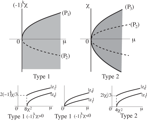
Figure 8: Domain of existence of bifurcating superposition of hexagons and rolls (balanced hexa-rolls types 1 and 2) for small $|\chi|$. Solutions of type 1 (three hexagon amplitudes equal at leading order) are on the left side, solutions of type 2 (two of the three hexagon amplitudes equal at leading order) are on the right side. The parabola $(P_{2})$ (dashed line) is a forbidden place.

Theorem 4.12 (Hexa-rolls: superposed hexagons and rolls in balance).

Assume that $\alpha\in{\mathcal{E}_{0}}$. Then, for $\chi=\varepsilon\kappa$, $\varepsilon>0$ close enough to 0, we can build a series in powers of $\varepsilon$, solution of Eq. 14, of the form

$$u(\varepsilon,\kappa,\Theta,k,j) = \varepsilon u_{1}(\Theta)+\sum_{n\geq 1}\varepsilon^{2n+1}u_{2n+1}(\kappa,\Theta,k,j),\text{ }u_{2n+1}\bot e^{i{\mathbf{k}}_{1}\cdot{\mathbf{x}}},\text{ }n\geq 1,$$

$$u_{1}(\Theta,\kappa,k,j) = \sum_{m=1,2}e^{i({\mathbf{k}}_{m}\cdot{\mathbf{x}}+\theta_{m})}+\zeta_{3}e^{i({\mathbf{k}}_{3}\cdot{\mathbf{x}}+\theta_{3})}+\sqrt{u_{4}^{(0)}}e^{i({\mathbf{k}}_{j}\cdot{\mathbf{x}}+\theta_{j})}+c.c.,$$

$$\Theta = (\theta_{1},\theta_{2},\theta_{3},\theta_{j}),\text{ }j=4\text{ or }5\text{ or }6,\text{ }\theta_{1}+\theta_{2}+\theta_{3}=k\pi,\text{ }k=0\text{ or }1$$

$$\mu(\varepsilon,\kappa,k,j) = \varepsilon^{2}\mu^{(0)}(\kappa,k)+\sum_{n\geq 2}\varepsilon^{2n}\mu_{2n}(\kappa,k,j),$$

Balanced hexa-rolls type 1 (three hexagon amplitudes equal at leading order):

$$\zeta_{3}=1,\text{ }\mu^{(0)}(\kappa,k)=(-1)^{k+1}2\kappa+21,\text{ }u_{4}^{(0)}=(-1)^{k+1}\frac{2}{3}\kappa+1,\text{ }(-1)^{k}\kappa<3/2,\text{ }(-1)^{k}\kappa\neq-3/2.$$

Balanced hexa-rolls type 2 (two of the three hexagon amplitudes equal at leading order):

$$\zeta_{3}=\frac{2}{3}\kappa(-1)^{k+1},\text{ }\mu^{(0)}(\kappa)=15+4\kappa^{2},\text{ }u_{4}^{(0)}=1+\frac{4}{9}\kappa^{2},\text{ }\kappa\neq\pm 3/2.$$

The freedom left for $\Theta$ corresponds to an arbitrary choice for translations $\mathbf{T}_{{\mathbf{\delta}}}$, as well for hexagons as for rolls (for $\theta_{j}$). In the quasiperiodic case ($\alpha\in{\mathcal{E}_{2}}$), these solutions give quasipatterns using the methods of [25]. See Fig. 8 for understanding the domain of bifurcating solutions in the plane $(\mu,\chi)$. Figure 7 shows quasiperiodic examples of $u_{1}$.

Remark 4.13.

As for hexa-rolls with rolls dominating, these solutions are new, even in the periodic case. Moreover, notice that in this case also we have the surprising freedom on shifts for the roll part, even in the periodic case. This follows from the reality of the 4-dimensional system.

5 Conclusion

We have shown the existence of new quasipattern solutions of the Swift–Hohenberg equation with quadratic as well as cubic nonlinearity: superposed hexagons with unequal amplitudes (valid only for small $\mu,\chi$). The existence of superposed hexagons with equal amplitudes ($\varepsilon=\pm\delta$) had already been established in [19, 25]. We have also found (provided the cubic coefficients satisfy an inequality) a new class of solutions, superposed hexagons and rolls: the roll amplitude dominates if the quadratic coefficient $\chi$ is not small, but for small $\chi=\mathcal{O}(\sqrt{|\mu|})$, the rolls and hexagons can have similar amplitudes. For small $\chi$, we have also found superposed symmetry-broken hexagons and rolls. Our approach relies on the small-divisor techniques from [25] for solutions of the amplitude equations to be translated into quasipattern solutions of the PDE Eq. 1. The end result is that for a full measure set of angles ($\alpha\in{\mathcal{E}_{2}}$), two hexagonal patterns with essentially arbitrary relative orientation and position can be superposed to produce quasipattern solutions of the Swift–Hohenberg equation. Similarly, superposed hexagons and rolls, again with essentially arbitrary relative orientation and position, also give quasipattern solutions.

In the periodic case we recover the superposed hexagon solutions already known from [15]. We have shown that the additional triangular superlattice solutions identified by [45] in the case $(a,b)=(3,2)$ also arise for general $(a,b)$. We find a new class of periodic superposed hexagon and roll solutions, provided the cubic coefficients satisfy an inequality and $a>b+1$. Surprisingly, even in the periodic case, the hexagons and rolls can be translated arbitrarily with respect to each other.

The approach we have taken differs from that familiar from equivariant bifurcation theory (which applies only in the periodic case). When the amplitude equations reduce to a single equation, the results are of course the same. The new solutions arise in cases where there is more than one equation to solve, and in some cases, these solutions have no symmetry. Our approach indicates how a wider class of pattern solutions can be investigated in pattern formation problems posed on the whole plane. It is likely that there are many other solutions still to be found: hexagons with superposed rhombuses dominating (see [49]), three sets of rolls at different angles to each other, superpositions of hexagons and squares, or squares and rolls at different angles, …. In all of these cases, careful consideration will have to be given to the Diophantine condition and to the behavior of high-order nonlinear modes.

We have not discussed stability of these quasipatterns: that is an important and difficult problem. However, the reason for including a quadratic term in the Swift–Hohenberg equation Eq. 1 is that three-wave interactions generated by quadratic terms, particularly in problems in which patterns on two length scales are simultaneously unstable, are known to play a key role in stabilizing quasipatterns in a variety of contexts [18, 31, 41, 34, 37, 56, 42, 47, 48, 39, 12, 4, 5]. Despite this, we do not expect any of the new solutions to be stable in the Swift–Hohenberg equation, but they (or related solutions) may be stable in other situations.

The recently discovered “bronze-mean hexagonal quasicrystals” described in [16, 36, 3] fall into the class of superposed hexagons. These quasicrystals are not solutions of a PDE, but rather are constructed from assemblies of three tiles: small equilateral triangles, large equilateral triangles, and rectangles. The Fourier transform of a six-fold aperiodic tiling made from these tiles has prominent peaks arranged as in Fig. 2(c), with $\alpha=25.66^{\circ}$, and the ideas presented here may be relevant to existence of this type of quasipattern in a pattern-forming PDE.

Finally, we mention a potential application of this body of work to bi-layer graphene, where two layers of hexagonally connected carbon atoms are superposed with a small orientation difference [53]: for $\alpha$ about $1^{\circ}$, these bi-layer structures can be superconducting [52]. Our work may be relevant for finding quasiperiodic structures in models of this system.

Appendix A Definitions of all the sets of angles

Here we first recall definitions given in main text, and supplement these with descriptions of ${\mathcal{E}_{1}}$ and ${\mathcal{E}_{2}}$.

The set ${\mathcal{E}_{p}}$ (periodic case) is given in Definition 2.1, and has $\cos\alpha$ and $\sqrt{3}\sin\alpha$ both rational, with $\alpha\in(0,\frac{\pi}{3})$. The complement of ${\mathcal{E}_{p}}$, restricted to $(0,\frac{\pi}{6}]$, is ${\mathcal{E}_{qp}}$ (quasiperiodic case). The set ${\mathcal{E}_{0}}$, given in Definition 2.4, is the set of angles $\alpha$ such that the only solutions of $|{\mathbf{k}}({\mathbf{m}})|=1$ are $\pm{\mathbf{k}}_{j}$, $j=1,\dots,6$.

The two sets ${\mathcal{E}_{1}}$ and ${\mathcal{E}_{2}}$ are defined in detail in [25] and described below: these are angles $\alpha\in{\mathcal{E}_{qp}}$ where additional Diophantine conditions are satisfied. The final set is ${\mathcal{E}_{2}}$.

Lemma 7 of [25] states that for nearly all $\alpha\in{\mathcal{E}_{qp}}\cap(0,\frac{\pi}{6}]$, and for any $\varepsilon>0$, there exists $c>0$ such that for all ${\mathbf{m}}\neq 0$ with $|{\mathbf{k}}({\mathbf{m}})|\neq 1$,

$$(|{\mathbf{k}}({\mathbf{m}})|^{2}-1)^{2}\geq\frac{c}{|N_{{\mathbf{k}}}|^{12+\varepsilon}}$$

holds. The set ${\mathcal{E}_{1}}$ is the set of all $\alpha$’s such that this inequality holds, and ${\mathcal{E}_{1}}$ is of full measure.

Let us now choose an integer $1\leq d\leq 4$ and consider an expression of the form

(47) $$P=a_{0}+\sum_{1\leq n\leq d}a_{n0}\cos^{n}\alpha+\sqrt{3}a_{n-1,1}\sin\alpha\cos^{n-1}\alpha,$$

where the coefficients $\mathbf{a}=(a_{0},a_{n0},a_{n-1,1},n=1,\dots,d)$ are integers: $\mathbf{a}\in\mathbb{Z}^{(2d+1)}$. The following proposition is proved in [25] (see Proposition 21):

Proposition A.1.

For nearly all $\alpha\in{\mathcal{E}_{0}}\cap{\mathcal{E}_{1}}\cap(0,\frac{\pi}{6}],$ there exists $c>0$ such that for all $\mathbf{a}\in\mathbb{Z}^{(2d+1)}\backslash\{0\}$ and for $l=2d(2d+1)$,

$$|P|\geq\frac{c}{|\mathbf{a}|^{l}},$$

where $\mathbf{a}=(a_{0},a_{n0},a_{n-1,1},n=1,\dots,d)$, $1\leq d\leq 4$, and

$$|\mathbf{a}|=|a_{0}|+\sum_{1\leq n\leq d}|a_{n0}|+|a_{n-1,1}|.$$

The set ${\mathcal{E}_{2}}$ is the set of all $\alpha\in(0,\frac{\pi}{6}]$ such that this inequality holds for any $d\leq 4$, provided that $|\mathbf{a}|\neq 0$. The set ${\mathcal{E}_{2}}$ is a subset of ${\mathcal{E}_{0}}\cap{\mathcal{E}_{1}}$, and ${\mathcal{E}_{2}}$ is of full measure [25].

Appendix B Proof of the properties of two example angles

While the set ${\mathcal{E}_{2}}$ is of full measure [25], in practice it can be difficult to determine whether any particular angle is or is not in the set. Here we take two examples and prove that $\alpha\approx 25.66^{\circ}$ ($\cos\alpha=\frac{1}{4}\sqrt{13}$) is in ${\mathcal{E}_{2}}$, while $\alpha\approx 26.44^{\circ}$ ($\cos\alpha=\frac{1}{12}(5+\sqrt{33})$) is not.

B.1 First example

Let us consider $\alpha\in{\mathcal{E}_{qp}}$ such that

$$\cos\alpha=\frac{\sqrt{13}}{4},\text{ \ }\sqrt{3}\sin\alpha=\frac{3}{4},$$

with $\alpha\approx 25.66^{\circ}$. In order to show that $\alpha\in{\mathcal{E}_{2}}$, we must first prove that $\alpha\in{\mathcal{E}_{0}}$, which means that the points of the lattice $\Gamma$ on the unit circle are only the twelve basic points $\pm{{\mathbf{k}}_{j}}$, $j=1,\dots,6$. For

$${\mathbf{k}}=n_{1}{\mathbf{k}}_{1}+n_{2}{\mathbf{k}}_{2}+n_{4}{\mathbf{k}}_{4}+n_{5}{\mathbf{k}}_{5},\text{ \ }n_{j}\in\mathbb{Z},$$

the condition $|{\mathbf{k}}|^{2}=1$ becomes

$$1 = n_{1}^{2}+n_{2}^{2}+n_{4}^{2}+n_{5}^{2}-n_{1}n_{2}-n_{4}n_{5}+{}$$

$${}+\cos\alpha(2n_{1}n_{4}+2n_{2}n_{5}-n_{1}n_{5}-n_{2}n_{4})+{}$$

$${}+\sqrt{3}\sin\alpha(n_{2}n_{4}-n_{1}n_{5}),$$

which, separating the rational and irrational parts, and with the given value of $\alpha$, leads to

(48) $$2n_{1}n_{4}+2n_{2}n_{5}-n_{1}n_{5}-n_{2}n_{4} =0,$$

$$3(n_{2}n_{4}-n_{1}n_{5})+4(n_{1}^{2}+n_{2}^{2}+n_{4}^{2}+n_{5}^{2}-n_{1}n_{2}-n_{4}n_{5}) =4.$$

Solving with respect to $n_{5}$ leads to

$$n_{5}=n_{4}\frac{n_{2}-2n_{1}}{2n_{2}-n_{1}},$$

provided that $n_{1}\neq 2n_{2}$,

$$0 = 4n_{4}^{2}\left(1+(\frac{n_{2}-2n_{1}}{2n_{2}-n_{1}})^{2}-\frac{n_{2}-2n_{1}}{2n_{2}-n_{1}}\right)+$$

$${}+3n_{4}\left(n_{2}-n_{1}\frac{n_{2}-2n_{1}}{2n_{2}-n_{1}}\right)+4(n_{1}^{2}+n_{2}^{2}-n_{1}n_{2}-1),$$

i.e.,

$$6n_{4}^{2}(n_{1}^{2}+n_{2}^{2}-n_{1}n_{2})+3n_{4}(n_{1}^{2}+n_{2}^{2}-n_{1}n_{2})(2n_{2}-n_{1})+2(n_{1}^{2}+n_{2}^{2}-n_{1}n_{2}-1)(2n_{2}-n_{1})^{2}=0.$$

The discriminant of this quadratic equation for $n_{4}$ reads

$$\Delta = 9(n_{1}^{2}+n_{2}^{2}-n_{1}n_{2})^{2}(2n_{2}-n_{1})^{2}-48(n_{1}^{2}+n_{2}^{2}-n_{1}n_{2}-1)(2n_{2}-n_{1})^{2}(n_{1}^{2}+n_{2}^{2}-n_{1}n_{2})$$

$$= 3(n_{1}^{2}+n_{2}^{2}-n_{1}n_{2})(2n_{2}-n_{1})^{2}\left[16-13(n_{1}^{2}+n_{2}^{2}-n_{1}n_{2})\right].$$

We observe that $\Delta$ should be $\geq 0$, and since $(n_{1}^{2}+n_{2}^{2}-n_{1}n_{2})(2n_{2}-n_{1})^{2}\geq 0$, this implies

$$16\geq 13(n_{1}^{2}+n_{2}^{2}-n_{1}n_{2}).$$

This in turn implies that

$$n_{1}^{2}+n_{2}^{2}-n_{1}n_{2}=1\text{ or }0.$$

The only solutions are

$$(n_{1},n_{2})=(0,0),(0,\pm 1),(\pm 1,0),(\pm 1,\pm 1),$$

leading to

$$\Delta = 9\text{ for }(n_{1},n_{2})=(\pm 1,0),(\pm 1,\pm 1),$$

$$\Delta = 36\text{ for }(n_{1},n_{2})=(0,\pm 1).$$

The case $(n_{1},n_{2})=(0,0)$ in Eq. 48, leads to $n_{4}^{2}+n_{5}^{2}-n_{4}n_{5}=1$, which correspond to $\pm{\mathbf{k}}_{4}$, $\pm{\mathbf{k}}_{5}$ and $\pm{\mathbf{k}}_{6}$. The case $(n_{1},n_{2})=(\pm 1,0),(\pm 1,\pm 1)$ leads to $n_{4}=0$ or $\mp\frac{1}{2}$ (which is not acceptable). Finally the case is $(n_{1},n_{2})=(0,\pm 1)$ gives

$$n_{4}=0\text{ or }\mp 1,$$

and $n_{5}=0$ or $\pm\frac{1}{2}$, and the only good possibility is $n_{4}=n_{5}=0$ and this corresponds to $\pm{\mathbf{k}}_{1},\pm{\mathbf{k}}_{2},\pm{\mathbf{k}}_{3}$. It remains to study the case $n_{1}=2n_{2}$, $n_{4}=0$. Replacing this in Eq. 48, we obtain

$$6n_{2}^{2}-3n_{2}n_{5}+2n_{5}^{2}-2=0$$

and it is easy to conclude that there are no other solutions of Eq. 48. The conclusion is that $\alpha\in{\mathcal{E}_{0}}$.

Let us now prove that $\alpha$ satisfies the two Diophantine conditions required in [25] and described in Appendix A. We observe that

$$4(|{\mathbf{k}}|^{2}-1) = q_{0}\sqrt{13}+q_{1},$$

$$q_{0} = 2n_{1}n_{4}+2n_{2}n_{5}-n_{1}n_{5}-n_{2}n_{4},$$

$$q_{1} = 3(n_{2}n_{4}-n_{1}n_{5})+4(n_{1}^{2}+n_{2}^{2}+n_{4}^{2}+n_{5}^{2}-n_{1}n_{2}-n_{4}n_{5})-4.$$

Since $\sqrt{13}$ is a quadratic irrational (the solution of a quadratic equation with integer coefficients), it is known [22] that there exists $C>0$ such that

$$|q_{0}\sqrt{13}+q_{1}|\geq\frac{C}{|q_{0}|+|q_{1}|},\text{ }(q_{0},q_{1})\in\mathbb{Z}^{2}\backslash\{0\}.$$

Since we have

$$|q_{0}| \leq \frac{3}{2}(n_{1}^{2}+n_{2}^{2}+n_{4}^{2}+n_{5}^{2}),$$

$$|q_{1}| \leq \frac{15}{2}(n_{1}^{2}+n_{2}^{2}+n_{4}^{2}+n_{5}^{2})+4$$

$$|q_{0}|+|q_{1}| \leq 11(n_{1}^{2}+n_{2}^{2}+n_{4}^{2}+n_{5}^{2}),$$

hence

$$(|{\mathbf{k}}|^{2}-1)^{2}\geq\frac{C^{\prime}}{(n_{1}^{2}+n_{2}^{2}+n_{4}^{2}+n_{5}^{2})^{2}},$$

which means that $\alpha\in{\mathcal{E}_{1}}$ as defined in [25] and described in Appendix A.

Now for ${\mathcal{E}_{2}}$, let us follow the lines of Appendix A. For this choice of $\alpha$, and for any integer $d\leq 4$, the expression Eq. 47 takes the form

$$P=\frac{b_{0}+b_{1}\sqrt{13}}{b_{2}},\text{ }b_{0},b_{1},b_{2}\in\mathbb{Z},$$

where the integer denominator depends on $\alpha$ and $d$ but not on the integers $\mathbf{a}$ in Eq. 47. Then, as soon as $|b_{0}|+|b_{1}|\neq 0$ we again have a Diophantine estimate

$$P>\frac{C^{\prime}}{|b_{0}|+|b_{1}|},$$

where $b_{2}$ is absorbed into $C^{\prime}$. This is the required property for $\alpha\in{\mathcal{E}_{2}}$ in [25] (see also Appendix A), and so the proof that $\alpha\in{\mathcal{E}_{2}}$ is complete. More generally if $\cos\alpha$ is rational and $\sqrt{3}\sin\alpha$ is a quadratic irrational, or vice versa, ${\mathcal{E}_{1}}$ should be satisfied, as should the Diophantine requirement of ${\mathcal{E}_{2}}$.

B.2 Second example

Let us consider $\alpha\in\mathcal{E}_{qp}$ such that

$$\cos\alpha=\frac{5+\sqrt{33}}{12},\text{ \ }\sqrt{3}\sin\alpha=\frac{15-\sqrt{33}}{12},$$

with $\alpha\approx 26.44^{\circ}$. We wish to prove that $\alpha\notin{\mathcal{E}_{2}}$. We have

$${\mathbf{k}}=n_{1}{\mathbf{k}}_{1}+n_{2}{\mathbf{k}}_{2}+n_{4}{\mathbf{k}}_{4}+n_{5}{\mathbf{k}}_{5},\text{ \ }n_{j}\in\mathbb{Z},$$

and, again separating rational and irrational parts, the condition $|{\mathbf{k}}|^{2}=1$ leads to

(49) $$0=3(n_{1}^{2}+n_{2}^{2}+n_{4}^{2}+n_{5}^{2}-n_{1}n_{2}-n_{4}n_{5}-1)+5(n_{2}n_{4}-n_{1}n_{5})$$

and

(50) $$n_{1}n_{4}+n_{2}n_{5}-n_{2}n_{4}=0.$$

Then we observe that

$$(n_{1},n_{2},n_{4},n_{5})=(2,1,-1,1)$$

is solution of Eq. 49, Eq. 50. This means that the following wave vectors lie on the unit circle

$$\pm({\mathbf{k}}_{1}-{\mathbf{k}}_{3}-{\mathbf{k}}_{4}+{\mathbf{k}}_{5})$$

$$\pm({\mathbf{k}}_{2}-{\mathbf{k}}_{1}-{\mathbf{k}}_{5}+{\mathbf{k}}_{6})$$

$$\pm({\mathbf{k}}_{3}-{\mathbf{k}}_{2}-{\mathbf{k}}_{6}+{\mathbf{k}}_{4})$$

and it is clear that $\pm{\mathbf{k}}_{j}$, $j=1,\dots,6$ are not the only elements of $\Gamma$ on the unit circle, so $\alpha\notin{\mathcal{E}_{0}}$ and $\alpha\notin{\mathcal{E}_{2}}$.

Appendix C Proof of Lemma 2.2

Let us show the following

Lemma C.1.

Let $\alpha\in{\mathcal{E}_{p}}\cap(0,\frac{\pi}{6})$, with $\cos\alpha$ and $\sqrt{3}\sin\alpha$ both rational, and define positive integers $p,q,p^{\prime}$ such that

(51) $$\cos\alpha=\frac{p}{q},\qquad\sqrt{3}\sin\alpha=\frac{p^{\prime}}{q},\qquad 3p^{2}+p^{\prime 2}=3q^{2},$$

where $(p,q,p^{\prime})$ have no common divisor. We define $d$ to be the greatest common divisor of $2(p+q)$ and $(p+q+p^{\prime})$. Then, $(a,b)$ defined by

(52) $$a=\frac{2(p+q)}{d},\qquad b=\frac{p+q+p^{\prime}}{d}$$

are relatively prime integers that satisfy Eq. 6 and $a>b>\tfrac{1}{2}a>0$.

Proof C.2.

Let us assume that Eq. 51 holds, and we seek integers $(a,b)$ such that Eq. 6 holds. If $(a,b)$ are integers given by Eq. 52, then (using $3p^{2}+p^{\prime 2}=3q^{2}$) this leads to

$$a^{2}+2ab-2b^{2} = p\times\frac{12(p+q)}{d^{2}},$$

$$3a(2b-a) = p^{\prime}\times\frac{12(p+q)}{d^{2}},$$

$$2(a^{2}-ab+b^{2}) = q\times\frac{12(p+q)}{d^{2}}.$$

Dividing the first and second lines by the third leads to Eq. 6. Now since $\alpha\in(0,\frac{\pi}{3})$ we have

$$p^{\prime}<\tfrac{{3}}{2}q<3p<3q,$$

which leads to

$$a>b>\tfrac{1}{2}a>0.$$

It remains to check that we can assume $a+b$ not multiple of $3$. Suppose that this is not the case, then we define

$$a^{\prime}=\tfrac{1}{3}(a+b),\qquad b^{\prime}=\tfrac{1}{3}(2a-b),$$

then it is easy to check that

$$\cos\left(\frac{\pi}{3}-\alpha\right)=\frac{a^{\prime 2}+2a^{\prime}b^{\prime}-2b^{\prime 2}}{2(a^{\prime 2}-a^{\prime}b^{\prime}+b^{\prime 2})},\qquad\sqrt{3}\sin\left(\frac{\pi}{3}-\alpha\right)=\frac{3a^{\prime}(2b^{\prime}-a^{\prime})}{2(a^{\prime 2}-a^{\prime}b^{\prime}+b^{\prime 2})},$$

hence we have for $\frac{\pi}{3}-\alpha$ the same formulas as for $\alpha$ in replacing $(a,b)$ by $(a^{\prime},b^{\prime})$. This means that in such a case we should choose to consider the angle $\alpha^{\prime}=\frac{\pi}{3}-\alpha$ instead of $\alpha$, which does not change the fact that $\alpha^{\prime}\in(0,\frac{\pi}{3})$. If it appears that $a^{\prime}+b^{\prime}$ is also multiple of 3, then we need to iterate the operation. In fact this operation means that we can choose basis vectors $(s_{1}-s_{2},s_{1}+2s_{2})$ instead of $(s_{1},s_{2})$, for the periodic lattice: these are $\sqrt{3}$ larger. The property (iii) of Lemma 2.2 is proved.

Now, we prove the density of $\mathcal{E}_{p}$. The continuous monotonous function of $x$

$$\frac{x^{2}+2x-2}{2(x^{2}-x+1)}$$

makes a homeomorphism between$(1,2)$ and $(\frac{1}{2},1)$, it is clear that the set of values taken by $\cos\alpha$ for $x=a/b$ rational is dense on $(\frac{1}{2},1)$. It follows that the set of angles $\alpha\in[0,\frac{\pi}{3})$ satisfying Eq. 6 for $a/b$ rational is dense. Hence the property (i) of Lemma 2.2 (the density of $\mathcal{E}_{p}$) is proved.

Remark C.3.

We notice that $d$ divides $2(p+q)$, and $2p^{\prime}$ and that $d^{2}$ divides $12(p+q)$ because $p,q$ and $p^{\prime}$ have no common divisor and $12(p+q)(q-p)=4p^{\prime 2}$

Appendix D Proof of Eq. 19

In this case the wave vectors ${\mathbf{k}}_{j}$ are defined in Eq. 7, and Eq. 17 leads to

$$(n_{1}-n_{3})a+(n_{2}-n_{3})(b-a)+(n_{4}-n_{6})a-(n_{5}-n_{6})b = 0,$$

$$(n_{1}-n_{3})b-(n_{2}-n_{3})a+(n_{4}-n_{6})(a-b)-(n_{5}-n_{6})a = 0.$$

Since $a$ and $b$ have no common factor, it follows that there exist $(j,l)\in\mathbb{Z}^{2}$ such that

$$n_{1}-n_{2}+n_{4}-n_{6} = jb,$$

$$n_{2}-n_{3}-n_{5}+n_{6} = -ja,$$

$$n_{2}-n_{3}-n_{4}+n_{5} = lb,$$

$$n_{1}-n_{3}-n_{4}+n_{6} = la.$$

This system leads to

$$n_{1}-n_{3} = jb+\frac{l-j}{3}(a+b),$$

$$n_{1}-n_{2} = la-\frac{l-j}{3}(a+b),$$

$$n_{4}-n_{5} = -ja-\frac{l-j}{3}(a+b),$$

$$n_{4}-n_{6} = jb-la+\frac{l-j}{3}(a+b).$$

Since $a+b$ is not a multiple of $3$, this implies that there is a $k\in\mathbb{Z}$ such that

$$l-j=3k,$$

and

$$n_{1}-n_{3} = (j+k)b+ka,$$

$$n_{1}-n_{2} = (j+2k)a-kb,$$

$$n_{4}-n_{5} = -(j+k)a-kb,$$

$$n_{4}-n_{6} = (j+k)b-(j+2k)a.$$

We notice that the monomials invariant under $\mathbf{T}_{{\mathbf{\delta}}}$, of minimal degree found in [15] correspond to the following choices: $(j,k)=(1,0),(-2,1),(1,-1)$, their complex conjugate being given by the opposite values of $(j,k)$. The basic invariant monomials where $a$ and $b$ occur are found by looking for the 27 monomials independent of two of the $z_{j}$:

$$q_{I,1}=z_{2}^{b}{\bar{z}}_{3}^{a-b}{\bar{z}}_{5}^{a-b}z_{6}^{b},\text{ \ }q_{I,2}={\bar{z}}_{2}^{a}{\bar{z}}_{3}^{b}z_{5}^{a}z_{6}^{a-b},\text{ \ }q_{I,3}=z_{2}^{a-b}z_{3}^{a}{\bar{z}}_{5}^{b}{\bar{z}}_{6}^{a},$$

$$q_{II,1}=z_{2}^{b}{\bar{z}}_{3}^{a-b}z_{4}^{a-b}z_{6}^{a},\text{ \ }q_{II,2}=z_{2}^{a-b}z_{3}^{a}z_{4}^{b}{\bar{z}}_{6}^{a-b},\text{ \ }q_{II,3}=z_{2}^{a}z_{3}^{b}z_{4}^{a}z_{6}^{b},$$

$$q_{III,1}=z_{2}^{a}z_{3}^{b}z_{4}^{a-b}{\bar{z}}_{5}^{b},\text{ \ }q_{III,2}=z_{2}^{b}{\bar{z}}_{3}^{a-b}{\bar{z}}_{4}^{b}{\bar{z}}_{5}^{a},\text{ \ }q_{III,3}=z_{2}^{a-b}z_{3}^{a}z_{4}^{a}z_{5}^{a-b},$$

$$q_{IV,1}=z_{1}^{b}z_{3}^{a}z_{5}^{a-b}{\bar{z}}_{6}^{b},\text{ \ }q_{IV,2}=z_{1}^{a-b}{\bar{z}}_{3}^{b}z_{5}^{b}z_{6}^{a},\text{ \ }q_{IV,3}=z_{1}^{a}z_{3}^{a-b}z_{5}^{a}z_{6}^{a-b},$$

$$q_{V,1}=z_{1}^{a-b}{\bar{z}}_{3}^{b}{\bar{z}}_{4}^{b}z_{6}^{a-b},\text{ \ }q_{V,2}=z_{1}^{a}z_{3}^{a-b}{\bar{z}}_{4}^{a}{\bar{z}}_{6}^{b},\text{ \ }q_{V,3}=z_{1}^{b}z_{3}^{a}{\bar{z}}_{4}^{a-b}{\bar{z}_{6}}^{a},$$

$$q_{VI,1}=z_{1}^{a}z_{3}^{a-b}{\bar{z}}_{4}^{a-b}z_{5}^{b},\text{ \ }q_{VI,2}=z_{1}^{a-b}{\bar{z}}_{3}^{b}{\bar{z}}_{4}^{a}{\bar{z}}_{5}^{a-b},\text{ \ }q_{VI,3}=z_{1}^{b}z_{3}^{a}z_{4}^{b}z_{5}^{a},$$

$$q_{VII,1}=z_{1}^{b}{\bar{z}}_{2}^{a-b}z_{5}^{a}z_{6}^{a-b},\text{ \ }q_{VII,2}=z_{1}^{a-b}z_{2}^{a}{\bar{z}}_{5}^{a-b}z_{6}^{b},\text{ \ }q_{VII,3}=z_{1}^{a}z_{2}^{b}z_{5}^{b}z_{6}^{a},$$

$$q_{VIII,1}=z_{1}^{b}{\bar{z}}_{2}^{a-b}{\bar{z}}_{4}^{a}{\bar{z}_{6}}^{b},\text{ \ }q_{VIII,2}=z_{1}^{a}z_{2}^{b}{\bar{z}}_{4}^{b}z_{6}^{a-b},\text{ \ }q_{VIII,3}=z_{1}^{a-b}z_{2}^{a}z_{4}^{a-b}z_{6}^{a},$$

$$q_{IX,1}=z_{1}^{b}{\bar{z}}_{2}^{a-b}{\bar{z}}_{4}^{a-b}z_{5}^{b},\text{ \ }q_{IX,2}=z_{1}^{a}z_{2}^{b}{\bar{z}}_{4}^{a}{\bar{z}}_{5}^{a-b},\text{ \ }q_{IX,3}=z_{1}^{a-b}z_{2}^{a}{\bar{z}}_{4}^{b}{\bar{z}_{5}}^{a}.$$

Notice that $q_{I,1}$, $q_{V,1}$, $q_{IX,1}$ are mentioned in [15]. We may also notice that these invariants are not independent since there are relationships between them and the $u_{j}$. We may group these invariant monomials into nine sets of monomials

$$G_{1} = \{q_{I,1},\overline{q_{V,1}},q_{IX,1}\}\text{ with degree }2a,$$

$$G_{2} = \{q_{II,1},\overline{q_{VI,2}},q_{VII,1}\}\text{ with degree }3a-b,$$

$$G_{2}^{\prime} = \{q_{II,2},q_{VI,1},q_{VII,2}\}\text{with degree }3a-b,$$

$$G_{3} = \{q_{III,1},q_{IV,1},q_{VIII,2}\}\text{ \ with degree }2a+b,$$

$$G_{3}^{\prime} = \{q_{III,2},\overline{q_{IV,2}},q_{VIII,1}\}\text{ with degree }2a+b,$$

$$G_{4} = \{q_{III,3},q_{IV,3},\text{ }q_{VIII,3}\}\text{ with degree }4a-2b,$$

$$G_{5} = \{\overline{q_{I,2}},q_{V,3},q_{IX,2}\}\text{ \ with degree }3a,$$

$$G_{5}^{\prime} = \{q_{I,3},q_{V,2},q_{IX,3}\}\text{, with degree }3a,$$

$$G_{6} = \{q_{II,3},q_{VI,3},q_{VII,3}\}\text{ with degree }2a+2b,$$

and their complex conjugates.

Let us control the action of various symmetries (other than $\mathbf{T}_{\delta}$, which leaves them invariant), useful for obtaining the system of 6 complex bifurcation equations. We have

$$\mathbf{R}_{\pi/3}\{q_{I,1},\overline{q_{V,1}},q_{IX,1}\} = \{q_{V,1},\overline{q_{IX,1}},\overline{q_{I,1}}\},$$

$$\mathbf{\tau}\{q_{I,1},\overline{q_{V,1}},q_{IX,1}\} = \{q_{I,1},q_{IX,1},\overline{q_{V,1}}\},$$

$$\mathbf{S}\{q_{I,1},\overline{q_{V,1}},q_{IX,1}\} = \{q_{I,1},\overline{q_{V,1}},q_{IX,1}\},$$

$$\mathbf{R}_{\pi/3}\{q_{II,1},\overline{q_{VI,2}},q_{VII,1}\} = \{q_{VI,2},\overline{q_{VII,1}},\overline{q_{II,1}}\},$$

$$\mathbf{\tau}\{q_{II,1},\overline{q_{VI,2}},q_{VII,1}\} = \{q_{VII,2},q_{VI,1},q_{II,2}\},$$

$$\mathbf{S}\{q_{II,1},\overline{q_{VI,2}},q_{VII,1}\} = (-1)^{a+b}\{q_{II,1},\overline{q_{VI,2}},q_{VII,1}\},$$

$$\mathbf{R}_{\pi/3}\{q_{II,2},q_{VI,1},q_{VII,2}\} = \{\overline{q_{VI,1}},\overline{q_{VII,2}},\overline{q_{II,2}}\},$$

$$\mathbf{\tau}\{q_{II,2},q_{VI,1},q_{VII,2}\} = \{q_{VII,1},\overline{q_{VI,2}},q_{II,1}\},$$

$$\mathbf{S}\{q_{II,2},q_{VI,1},q_{VII,2}\} = (-1)^{a+b}\{q_{II,2},q_{VI,1},q_{VII,2}\},$$

$$\mathbf{R}_{\pi/3}\{q_{III,1},q_{IV,1},q_{VIII,2}\} = \{\overline{q_{IV,1}},\overline{q_{VIII,2}},\overline{q_{III,1}}\},$$

$$\mathbf{\tau}\{q_{III,1},q_{IV,1},q_{VIII,2}\} = \{q_{IV,2},\overline{q_{III,2}},\overline{q_{VIII,1}}\},$$

$$\mathbf{S}\{q_{III,1},q_{IV,1},q_{VIII,2}\} = (-1)^{b}\{q_{III,1},q_{IV,1},q_{VIII,2}\},$$

$$\mathbf{R}_{\pi/3}\{q_{III,2},\overline{q_{IV,2}},q_{VIII,1}\} = \{q_{IV,2},\overline{q_{VIII,1}},\overline{q_{III,2}}\},$$

$$\mathbf{\tau}\{q_{III,2},\overline{q_{IV,2}},q_{VIII,1}\} = \{\overline{q_{IV,1}},\overline{q_{III,1}},\overline{q_{VIII,2}}\},$$

$$\mathbf{S}\{q_{III,2},\overline{q_{IV,2}},q_{VIII,1}\} = (-1)^{b}\{q_{III,2},\overline{q_{IV,2}},q_{VIII,1}\},$$

$$\mathbf{R}_{\pi/3}\{q_{III,3},q_{IV,3},q_{VIII,3}\} = \{\overline{q_{IV,3}},\overline{q_{VIII,3}},\overline{q_{III,3}}\},$$

$$\mathbf{\tau}\{q_{III,3},q_{IV,3},q_{VIII,3}\} = \{q_{IV,3},q_{III,3},q_{VIII,3}\},$$

$$\mathbf{S}\{q_{III,3},q_{IV,3},q_{VIII,3}\} = \{q_{III,3},q_{IV,3},q_{VIII,3}\},$$

$$\mathbf{R}_{\pi/3}\{\overline{q_{I,2}},q_{V,3},q_{IX,2}\} = \{\overline{q_{V,3}},\overline{q_{IX,2}},q_{I,2}\},$$

$$\mathbf{\tau}\{\overline{q_{I,2}},q_{V,3},q_{IX,2}\} = \{\overline{q_{I,3}},\overline{q_{IX,3}},\overline{q_{V,2}}\},$$

$$\mathbf{S}\{\overline{q_{I,2}},q_{V,3},q_{IX,2}\} = (-1)^{a}\{\overline{q_{I,2}},q_{V,3},q_{IX,2}\},$$

$$\mathbf{R}_{\pi/3}\{q_{I,3},q_{V,2},q_{IX,3}\} = \{\overline{q_{V,2}},\overline{q_{IX,3}},\overline{q_{I,3}}\},$$

$$\mathbf{\tau}\{q_{I,3},q_{V,2},q_{IX,3}\} = \{q_{I,2},\overline{q_{IX,2}},\overline{q_{V,3}}\},$$

$$\mathbf{S}\{q_{I,3},q_{V,2},q_{IX,3}\} = (-1)^{a}\{q_{I,3},q_{V,2},q_{IX,3}\},$$

$$\mathbf{R}_{\pi/3}\{q_{II,3},q_{VI,3},q_{VII,3}\} = \{\overline{q_{VI,3}},\overline{q_{VII,3}},\overline{q_{II,3}}\},$$

$$\mathbf{\tau}\{q_{II,3},q_{VI,3},q_{VII,3}\} = \{q_{VII,3},q_{VI,3},q_{II,3}\},$$

$$\mathbf{S}\{q_{II,3},q_{VI,3},q_{VII,3}\} = \{q_{II,3},q_{VI,3},q_{VII,3}\}.$$

All this leads in a straightforward way to Eq. 19.

Appendix E Form of the cubic part of the bifurcation system

Equation Eq. 14, projected orthogonally on the complement of $\ker\mathbf{L}_{0}$, leads to

(53) $$\widetilde{\mathbf{L}_{0}}w=\mu w-\chi\mathbf{Q}_{0}(v_{1}+w)^{2}-\mathbf{Q}_{0}(v_{1}+w)^{3},$$

where we set

$$u=v_{1}+w,\text{ }v_{1}\in\ker\mathbf{L}_{0},\text{ }w\in\{\ker\mathbf{L}_{0}\}^{\bot},$$

and $\mathbf{Q}_{0}$ is the orthogonal projection on the complement of $\ker\mathbf{L}_{0}$, $\widetilde{\mathbf{L}_{0}}$ being the restriction of $\mathbf{L}_{0}$ on its range, the inverse of which is the pseudo-inverse of $\mathbf{L}_{0}$ (bounded in the periodic case, unbounded in the quasiperiodic case because of small divisors). Equation Eq. 53 may be solved formally with respect to $w$ as a power series in $v_{1}$ and $\mu$. We have at quadratic order

$$w_{2}=-\chi\widetilde{\mathbf{L}_{0}}^{-1}\mathbf{Q}_{0}v_{1}^{2},$$

and at cubic order in $v_{1},\mu$

$$w_{3}=-\mu\chi\widetilde{\mathbf{L}_{0}}^{-2}\mathbf{Q}_{0}v_{1}^{2}+2\chi^{2}\widetilde{\mathbf{L}_{0}}^{-1}\mathbf{Q}_{0}[v_{1}\widetilde{\mathbf{L}_{0}}^{-1}\mathbf{Q}_{0}v_{1}^{2}]-\widetilde{\mathbf{L}_{0}}^{-1}\mathbf{Q}_{0}v_{1}^{3}.$$

Now the bifurcation equation is

$$0=\mu v_{1}-\chi\mathbf{P}_{0}(v_{1}+w)^{2}-\mathbf{P}_{0}(v_{1}+w)^{3},$$

where $\mathbf{P}_{0}$ is the orthogonal projection on $\ker\mathbf{L}_{0}$ and where we replace $w$ by its formal expansion in powers of $(\mu,v_{1})$. This leads to

$$\mu v_{1}=\chi\mathbf{P}_{0}v_{1}^{2}+\mathbf{P}_{0}v_{1}^{3}-2\chi^{2}\mathbf{P}_{0}v_{1}\widetilde{\mathbf{L}_{0}}^{-1}\mathbf{Q}_{0}v_{1}^{2}+\mathcal{O}(v_{1}^{4}).$$

It follows that, up to cubic order in $(\mu,v_{1})$, the bifurcation system reads

$$\mu v_{1}=\chi\mathbf{P}_{0}v_{1}^{2}+\mathbf{P}_{0}v_{1}^{3}-2\chi^{2}\mathbf{P}_{0}v_{1}\widetilde{\mathbf{L}_{0}}^{-1}\mathbf{Q}_{0}v_{1}^{2}.$$

The scalar product with $e^{i{\mathbf{k}}_{1}\cdot{\mathbf{x}}}$ gives

(54) $$\mu z_{1}=\chi\langle v_{1}^{2},e^{i{\mathbf{k}}_{1}\cdot{\mathbf{x}}}\rangle+\langle v_{1}^{3},e^{i{\mathbf{k}}_{1}\cdot{\mathbf{x}}}\rangle-2\chi^{2}\langle v_{1}\widetilde{\mathbf{L}_{0}}^{-1}\mathbf{Q}_{0}v_{1}^{2},e^{i{\mathbf{k}}_{1}\cdot{\mathbf{x}}}\rangle.$$

It is straightforward to check that

$$\langle v_{1}^{2},e^{i{\mathbf{k}}_{1}\cdot{\mathbf{x}}}\rangle=2\overline{z_{2}}\overline{z_{3}},$$

$$\langle v_{1}^{3},e^{i{\mathbf{k}}_{1}\cdot{\mathbf{x}}}\rangle = \langle 3z_{1}^{2}\overline{z_{1}}e^{i{\mathbf{k}}_{1}\cdot{\mathbf{x}}}+6\sum_{j=2,\dots,6}z_{1}z_{j}\overline{z_{j}}e^{i{\mathbf{k}}_{1}\cdot{\mathbf{x}}},e^{i{\mathbf{k}}_{1}\cdot{\mathbf{x}}}\rangle$$

$$= 3z_{1}u_{1}+6z_{1}(u_{2}+u_{3}+u_{4}+u_{5}+u_{6}).$$

The next term is more complicated:

$$\langle v_{1}\widetilde{\mathbf{L}_{0}}^{-1}\mathbf{Q}_{0}v_{1}^{2},e^{i{\mathbf{k}}_{1}\cdot{\mathbf{x}}}\rangle=\sum_{j=1,\dots,6}z_{j}\langle\widetilde{\mathbf{L}_{0}}^{-1}\mathbf{Q}_{0}v_{1}^{2},e^{i({\mathbf{k}}_{1}-{\mathbf{k}}_{j})\cdot{\mathbf{x}}}\rangle+\sum_{j=1,\dots,6}\overline{z_{j}}\langle\widetilde{\mathbf{L}_{0}}^{-1}\mathbf{Q}_{0}v_{1}^{2},e^{i({\mathbf{k}}_{1}+{\mathbf{k}}_{j})\cdot{\mathbf{x}}}\rangle,$$

and the relevant terms in $v_{1}^{2}$ are those with an exponent

$$({\mathbf{k}}_{1}\mp{\mathbf{k}}_{j})\cdot{\mathbf{x}},\text{ such that }{\mathbf{k}}_{1}\mp{\mathbf{k}}_{j}\neq\pm{\mathbf{k}}_{l},\text{ }l=1,\dots,6.$$

the operator $\widetilde{\mathbf{L}_{0}}^{-1}$ provides a multiplication by

$$(1-|{\mathbf{k}}_{1}\mp{\mathbf{k}}_{j}|^{2})^{-2}.$$

We notice that

$$|{\mathbf{k}}_{1}-{\mathbf{k}}_{2}| = |{\mathbf{k}}_{1}-{\mathbf{k}}_{3}|,\text{ while }|{\mathbf{k}}_{1}+{\mathbf{k}}_{2}|,|{\mathbf{k}}_{1}+{\mathbf{k}}_{3}|\text{ do not appear,}$$

$$|{\mathbf{k}}_{1}\pm{\mathbf{k}}_{4}|,|{\mathbf{k}}_{1}\pm{\mathbf{k}}_{5}|,|{\mathbf{k}}_{1}\pm{\mathbf{k}}_{6}|\text{ all different and functions of }\alpha.$$

Hence

$$2\chi^{2}\langle v_{1}\widetilde{\mathbf{L}_{0}}^{-1}\mathbf{Q}_{0}v_{1}^{2},e^{i{\mathbf{k}}_{1}\cdot{\mathbf{x}}}\rangle=\chi^{2}z_{1}[c_{1}u_{1}+c_{2}(u_{2}+u_{3})+c_{\alpha}u_{4}+c_{\alpha+}u_{5}+c_{\alpha-}u_{6}],$$

with

$$c_{1} = 2(1+1/9),\text{ since }|2{\mathbf{k}}_{1}|=2,$$

$$c_{2} = 2(1+1/2),\text{ since }|{\mathbf{k}}_{1}-{\mathbf{k}}_{2}|=\sqrt{3},$$

$$c_{\alpha} = 2[1+2(1-|{\mathbf{k}}_{1}-{\mathbf{k}}_{4}|^{2})^{-2}+2(1-|{\mathbf{k}}_{1}+{\mathbf{k}}_{4}|^{2})^{-2}],$$

$$c_{\alpha+} = 2[1+2(1-|{\mathbf{k}}_{1}-{\mathbf{k}}_{5}|^{2})^{-2}+2(1-|{\mathbf{k}}_{1}+{\mathbf{k}}_{5}|^{2})^{-2}],$$

$$c_{\alpha-} = 2[1+2(1-|{\mathbf{k}}_{1}-{\mathbf{k}}_{6}|^{2})^{-2}+2(1-|{\mathbf{k}}_{1}+{\mathbf{k}}_{6}|^{2})^{-2}].$$

Appendix F Looking for translations

Let us consider the cases with $\alpha\in{\mathcal{E}_{p}}$, then we can choose the translation operator $\mathbf{T}_{\mathbf{\delta}}$ such that

(55) $$\mathbf{\delta}\cdot{\mathbf{k}}_{j} =\phantom{-}\frac{2\pi}{3}\mod 2\pi,\text{ for }j=1,2,3,$$

$$=-\frac{2\pi}{3}\mod 2\pi,\text{ for }j=4,5,6.$$

Indeed, we set

$$\mathbf{\delta}=\frac{2\pi}{3}\lambda^{2}m\mathbf{s}_{1},$$

where $\mathbf{s}_{1}$ and $\lambda$ are defined at Lemma 2.2 and $m$ is an integer. Then Eq. 55 leads to

$$m(2a-b) = 2(1+3n_{1}),$$

$$m(2b-a) = 2(1+3n_{2}),$$

$$m(a+b) = 2(-1+3n_{4}),$$

$$m(a-2b) = 2(-1+3n_{5}),$$

where $n_{1},n_{2},n_{4},n_{5}$ are integers. It follows that

$$n_{2}+n_{5} = 0,$$

$$am = 2(n_{1}+n_{4}),$$

$$a(2n_{4}-n_{1}-1) = b(n_{1}+n_{4}),$$

$$a(n_{1}+n_{4}+3n_{2}+1) = 2b(n_{1}+n_{4}).$$

The last two lines give

$$n_{2}=n_{4}-n_{1}-1,$$

and so

$$n_{1}+n_{4} = la,$$

$$2n_{4}-n_{1}-1 = lb,$$

where $l$ is an integer, leading to

$$3n_{4}=1+l(a+b).$$

Since $a+b$ is not multiple of 3, we have to look at two cases: $a+b=3j+1$  or $a+b=3j+2$.

For $a+b=3j+1$ we choose $l=2$, hence

$$n_{4}=2j+1,\text{ }n_{1}=2a-2j-1,\text{ }n_{2}=4j-2a+1,\text{ }n_{5}=-n_{2},\text{ }m=4.$$

For $a+b=3j+2$ we choose $l=1$, hence

$$n_{4}=j+1,\text{ }n_{1}=a-j-1,\text{ }n_{2}=2j-a+1,\text{ }n_{5}=-n_{2},\text{ }m=2.$$

It follows that the solutions in Theorem 4.5 obtained for $\theta_{1}=\theta_{2}=\theta_{3}=-\theta_{4}=-\theta_{5}=-\theta_{6}=k\frac{\pi}{3}$, provide only two different patterns, one corresponding to $k=0,2,4$, the other for $k=1,3,5$.

References

- [1] C. V. Achim, M. Schmiedeberg, and H. Löwen, Growth modes of quasicrystals, Phys. Rev. Lett., 112 (2014), p. 255501, https://doi.org/10.1103/PhysRevLett.112.255501.
- [2] H. Arbell and J. Fineberg, Pattern formation in two-frequency forced parametric waves, Phys. Rev. E, 65 (2002), p. 036224, https://doi.org/10.1103/PhysRevE.65.036224.
- [3] A. J. Archer, T. Dotera, and A. M. Rucklidge, Rectangle–triangle soft-matter quasicrystals with hexagonal symmetry, in preparation, (2021).
- [4] A. J. Archer, A. M. Rucklidge, and E. Knobloch, Quasicrystalline order and a crystal-liquid state in a soft-core fluid, Phys. Rev. Lett., 111 (2013), p. 165501, https://doi.org/10.1103/PhysRevLett.111.165501.
- [5] M. Argentina and G. Iooss, Quasipatterns in a parametrically forced horizontal fluid film, Physica D, 241 (2012), pp. 1306–1321, https://doi.org/10.1016/j.physd.2012.04.011.
- [6] A. Aumann, T. Ackemann, E. G. Westhoff, and W. Lange, Eightfold quasipatterns in an optical pattern-forming system, Phys. Rev. E, 66 (2002), p. 046220, https://doi.org/10.1103/PhysRevE.66.046220.
- [7] M. Baake and U. Grimm, Mathematical diffraction of aperiodic structures, Chem. Soc. Rev., 41 (2012), pp. 6821–6843, https://doi.org/https://doi.org/10.1039/C2CS35120J.
- [8] K. Barkan, M. Engel, and R. Lifshitz, Controlled self-assembly of periodic and aperiodic cluster crystals, Phys. Rev. Lett., 113 (2014), p. 098304, https://doi.org/10.1103/PhysRevLett.113.098304.
- [9] B. Braaksma and G. Iooss, Existence of bifurcating quasipatterns in steady Bénard–Rayleigh convection, Arch. Ration. Mech. Anal., 231 (2019), pp. 1917–1981, https://doi.org/10.1007/s00205-018-1313-6.
- [10] B. Braaksma, G. Iooss, and L. Stolovitch, Proof of quasipatterns for the Swift–Hohenberg equation, Commun. Math. Phys., 353 (2017), pp. 37–67, https://doi.org/10.1007/s00220-017-2878-x.
- [11] J. Carr, Applications of Centre Manifold Theory, Springer, New York, 1981.
- [12] J. K. Castelino, D. J. Ratliff, A. M. Rucklidge, P. Subramanian, and C. M. Topaz, Spatiotemporal chaos and quasipatterns in coupled reaction–diffusion systems, Physica D, 407 (2020), p. 132475, https://doi.org/10.1016/j.physd.2020.132475.
- [13] J. D. Crawford, mode interactions and hidden rotational symmetry, Nonlinearity, 7 (1994), pp. 697–739, https://doi.org/10.1088/0951-7715/7/3/002.
- [14] J. H. P. Dawes, P. C. Matthews, and A. M. Rucklidge, Reducible actions of : superlattice patterns and hidden symmetries, Nonlinearity, 16 (2003), pp. 615–645, https://doi.org/10.1088/0951-7715/16/2/315.
- [15] B. Dionne, M. Silber, and A. C. Skeldon, Stability results for steady, spatially periodic planforms, Nonlinearity, 10 (1997), pp. 321–353, https://doi.org/10.1088/0951-7715/10/2/002.
- [16] T. Dotera, S. Bekku, and P. Ziherl, Bronze-mean hexagonal quasicrystal, Nature Mat., 16 (2017), pp. 987–992, https://doi.org/10.1038/nmat4963.
- [17] B. Echebarria and H. Riecke, Sideband instabilities and defects of quasipatterns, Physica D, 158 (2001), pp. 45–68, https://doi.org/10.1016/S0167-2789(01)00319-0.
- [18] W. S. Edwards and S. Fauve, Patterns and quasi-patterns in the Faraday experiment, J. Fluid Mech., 278 (1994), pp. 123–148, https://doi.org/10.1017/S0022112094003642.
- [19] S. Fauve and G. Iooss, Quasipatterns versus superlattices resulting from the superposition of two hexagonal patterns, Comptes Rendus Mecanique, 347 (2019), pp. 294–304, https://doi.org/10.1016/j.crme.2019.03.006.
- [20] A. Gökçe, S. Coombes, and D. Avitabile, Quasicrystal patterns in a neural field model, Phys. Rev. Research, 2 (2020), p. 013234, https://doi.org/10.1103/PhysRevResearch.2.013234.
- [21] M. Golubitsky, I. Stewart, and D. G. Schaeffer, Singularities and Groups in Bifurcation Theory. Volume II, Springer, New York, 1988.
- [22] G. H. Hardy and E. M. Wright, An Introduction to the Theory of Numbers, Clarendon Press, Oxford, 4th ed., 1960.
- [23] K. Hayashida, T. Dotera, A. Takano, and Y. Matsushita, Polymeric quasicrystal: Mesoscopic quasicrystalline tiling in star polymers, Phys. Rev. Lett., 98 (2007), p. 195502, https://doi.org/10.1103/PhysRevLett.98.195502.
- [24] R. B. Hoyle, Pattern Formation: an Introduction to Methods, Cambridge University Press, Cambridge, 2006.
- [25] G. Iooss, Existence of quasipatterns in the superposition of two hexagonal patterns, Nonlinearity, 32 (2019), pp. 3163–3187, https://doi.org/10.1088/1361-6544/ab230a.
- [26] G. Iooss and A. M. Rucklidge, On the existence of quasipattern solutions of the Swift–Hohenberg equation, J. Nonlin. Sci., 20 (2010), pp. 361–394, https://doi.org/10.1007/s00332-010-9063-0.
- [27] K. Jiang, J. Tong, P. Zhang, and A.-C. Shi, Stability of two-dimensional soft quasicrystals in systems with two length scales, Phys. Rev. E, 92 (2015), p. 042159, https://doi.org/10.1103/PhysRevE.92.042159.
- [28] Z. Jiang, S. Quan, N. Xu, L. He, and Y. Ni, Growth modes of quasicrystals involving intermediate phases and a multistep behavior studied by phase field crystal model, Phys. Rev. Materials, 4 (2020), p. 023403, https://doi.org/10.1103/PhysRevMaterials.4.023403.
- [29] A. Kudrolli, B. Pier, and J. P. Gollub, Superlattice patterns in surface waves, Physica D, 123 (1998), pp. 99–111, https://doi.org/10.1103/10.1016/S0167-2789(98)00115-8.
- [30] R. Lifshitz and H. Diamant, Soft quasicrystals – Why are they stable?, Philos. Mag., 87 (2007), pp. 3021–3030, https://doi.org/10.1080/14786430701358673.
- [31] R. Lifshitz and D. M. Petrich, Theoretical model for Faraday waves with multiple-frequency forcing, Phys. Rev. Lett., 79 (1997), pp. 1261–1264, https://doi.org/10.1103/PhysRevLett.79.1261.
- [32] B. A. Malomed, A. A. Nepomnyashchiĭ, and M. I. Tribelskiĭ, Two-dimensional quasiperiodic structures in nonequilibrium systems, Sov. Phys. JETP, 69 (1989), pp. 388–396.
- [33] P. C. Matthews, Transcritical bifurcation with symmetry, Nonlinearity, 16 (2003), pp. 1449–1471, https://doi.org/10.1088/0951-7715/16/4/315.
- [34] N. D. Mermin and S. M. Troian, Mean-field theory of quasicrystalline order, Phys. Rev. Lett., 54 (1985), pp. 1524–1527, https://doi.org/10.1103/PhysRevLett.54.1524.
- [35] H. W. Müller, Model equations for two-dimensional quasipatterns, Phys. Rev. E, 49 (1994), pp. 1273–1277, https://doi.org/10.1103/PhysRevE.49.1273.
- [36] J. Nakakura, P. Ziherl, J. Matsuzawa, and T. Dotera, Metallic-mean quasicrystals as aperiodic approximants of periodic crystals, Nature Comm., 10 (2019), pp. 1–8, https://doi.org/10.1038/s41467-019-12147-z.
- [37] A. C. Newell and Y. Pomeau, Turbulent crystals in macroscopic systems, J. Phys. A, 26 (1993), pp. L429–L434, https://doi.org/10.1088/0305-4470/26/8/006.
- [38] J. Porter, C. M. Topaz, and M. Silber, Pattern control via multifrequency parametric forcing, Phys. Rev. Lett., 93 (2004), p. 034502, https://doi.org/10.1103/PhysRevLett.93.034502.
- [39] D. J. Ratliff, A. J. Archer, P. Subramanian, and A. M. Rucklidge, Which wave numbers determine the thermodynamic stability of soft matter quasicrystals?, Phys. Rev. Lett., 123 (2019), p. 148004, https://doi.org/10.1103/PhysRevLett.123.148004.
- [40] A. M. Rucklidge and W. J. Rucklidge, Convergence properties of the 8, 10 and 12 mode representations of quasipatterns, Physica D, 178 (2003), pp. 62–82, https://doi.org/10.1016/S0167-2789(02)00792-3.
- [41] A. M. Rucklidge and M. Silber, Design of parametrically forced patterns and quasipatterns, SIAM J. Appl. Dynam. Syst., 8 (2009), pp. 298–347, https://doi.org/10.1137/080719066.
- [42] A. M. Rucklidge, M. Silber, and A. C. Skeldon, Three-wave interactions and spatiotemporal chaos, Phys. Rev. Lett., 108 (2012), p. 074504, https://doi.org/10.1103/PhysRevLett.108.074504.
- [43] S. Savitz, M. Babadi, and R. Lifshitz, Multiple-scale structures: from Faraday waves to soft-matter quasicrystals, IUCrJ, 5 (2018), pp. 247–268, https://doi.org/10.1107/S2052252518001161.
- [44] D. Shechtman, I. Blech, D. Gratias, and J. W. Cahn, Metallic phase with long-range orientational order and no translational symmetry, Phys. Rev. Lett., 53 (1984), pp. 1951–1953, https://doi.org/10.1103/PhysRevLett.53.1951.
- [45] M. Silber and M. R. E. Proctor, Nonlinear competition between small and large hexagonal patterns, Phys. Rev. Lett., 81 (1998), pp. 2450–2453, https://doi.org/10.1103/PhysRevLett.81.2450.
- [46] A. C. Skeldon and G. Guidoboni, Pattern selection for Faraday waves in an incompressible viscous fluid, SIAM J. Appl. Math., 67 (2007), pp. 1064–1100, https://doi.org/10.1137/050639223.
- [47] A. C. Skeldon and A. M. Rucklidge, Can weakly nonlinear theory explain Faraday wave patterns near onset?, J. Fluid Mech., 777 (2015), pp. 604–632, https://doi.org/10.1017/jfm.2015.388.
- [48] P. Subramanian, A. J. Archer, E. Knobloch, and A. M. Rucklidge, Three-dimensional icosahedral phase field quasicrystal, Phys. Rev. Lett., 117 (2016), p. 075501, https://doi.org/10.1103/PhysRevLett.117.075501.
- [49] P. Subramanian, I. G. Kevrekidis, and P. G. Kevrekidis, Exploring critical points of energy landscapes: From low-dimensional examples to phase field crystal pdes, Commun. Nonlinear Sci. Numer. Simulat., 96 (2021), p. 105679, https://doi.org/10.1016/j.cnsns.2020.105679.
- [50] J. Swift and P. C. Hohenberg, Hydrodynamic fluctuations at the convective instability, Phys. Rev. A, 15 (1977), pp. 319–328, https://doi.org/10.1103/PhysRevA.15.319.
- [51] A. Vanderbauwhede and G. Iooss, Center manifold theory in infinite dimensions, in Dynamics Reported: Expositions in Dynamical Systems (New Series), C. Jones, K. U., and H. O. Walther, eds., vol. 1, Springer, Berlin, 1992, pp. 125–163.
- [52] M. Yankowitz, S. Chen, H. Polshyn, Y. Zhang, K. Watanabe, T. Taniguchi, D. Graf, A. F. Young, and C. R. Dean, Tuning superconductivity in twisted bilayer graphene, Science, 363 (2019), pp. 1059–1064, https://doi.org/10.1126/science.aav1910.
- [53] P. Zeller and S. Günther, What are the possible moiré patterns of graphene on hexagonally packed surfaces? Universal solution for hexagonal coincidence lattices, derived by a geometric construction, New J. Phys., 16 (2014), p. 083028, https://doi.org/10.1088/1367-2630/16/8/083028.
- [54] X. B. Zeng, G. Ungar, Y. S. Liu, V. Percec, S. E. Dulcey, and J. K. Hobbs, Supramolecular dendritic liquid quasicrystals, Nature, 428 (2004), pp. 157–160, https://doi.org/10.1038/nature02368.
- [55] W. B. Zhang and J. Viñals, Square patterns and quasipatterns in weakly damped Faraday waves, Phys. Rev. E, 53 (1996), pp. R4283–R4286, https://doi.org/10.1103/PhysRevE.53.R4283.
- [56] W. B. Zhang and J. Viñals, Pattern formation in weakly damped parametric surface waves driven by two frequency components, J. Fluid Mech., 341 (1997), pp. 225–244, https://doi.org/10.1017/S0022112097005387.