Statistical guarantees for generative models without domination

Abstract

In this paper, we introduce a convenient framework for studying (adversarial) generative models from a statistical perspective. It consists in modeling the generative device as a smooth transformation of the unit hypercube of a dimension that is much smaller than that of the ambient space and measuring the quality of the generative model by means of an integral probability metric. In the particular case of integral probability metric defined through a smoothness class, we establish a risk bound quantifying the role of various parameters. In particular, it clearly shows the impact of dimension reduction on the error of the generative model.

1 Introduction

The problem of learning generative models has attracted a lot of attention during the last 5 years in machine learning and artificial intelligence. The most prominent example is generating artificial images that look similar to actual photographs, by means of generative adversarial networks. The more general formulation of the problem can be given as a game between the user and the learner. The user samples a set of elements (images of natural scenes, poems, pieces of music, etc.) from a hidden distribution $P^{*}=P_{\textup{user}}$ defined on a hidden (and not so well known) space. The learner receives a noisy and possibly contaminated version of these elements and aims at generating a new set of elements, that are different from those transmitted by the user, but that could have been sampled from the hidden distribution $P^{*}$. Note that the revealed elements are usually of very high dimension. However, they may exhibit rich structures such as the harmonic and rhythmic schemes followed by a melody or a poem, or the presence of simple shapes in an image. It is therefore reasonable to assume that these elements can be represented by means of a much lower dimensional latent variable, which is unobserved.

In other words, generative models are used for accomplishing the following task. The user draws $n$ independent samples $\boldsymbol{Y}_{1},\ldots,\boldsymbol{Y}_{n}$ from a distribution $P_{\textup{user}}$ defined on $\mathbb{R}^{D}$. The learner is given a noisy and contaminated version $\boldsymbol{X}_{1},\ldots,\boldsymbol{X}_{n}$ of this sample. The goal of the learner is to design an algorithm that generates random samples from a distribution $P_{\textup{learner}}$ which is as close as possible to $P_{\textup{user}}$. This can be viewed as a distribution estimation problem with two requirements:

• It should be easy to sample from $P_{\textup{\rm learner}}$.

• The way we measure the closeness between $P_{\textup{\rm learner}}$ and $P_{\textup{\rm user}}$ for evaluating the error has to admit an interpretation as a sampling error.

Of course, this formulation is incomplete since it allows to take the uniform distribution over the observed samples as $P_{\textup{learner}}$, i.e., $P_{\textup{learner}}=\widehat{P}_{n}=\frac{1}{n}\sum_{i=1}^{n}\delta_{\boldsymbol{X}_{i}}$ (the empirical distribution based on the sample $\boldsymbol{X}_{1},\ldots,\boldsymbol{X}_{n}$). From a generative modeling perspective, $\widehat{P}_{n}$ is pointless since it does not yield new samples that are different from the previous ones. Hence, generative modeling requires a third distinctive feature:

• Samples drawn from $P_{\textup{learner}}$ should be different from those revealed by the user.

Requirement R3R3 is perhaps the hardest to translate into a statistical language. Most prior work focused on the case where both $P_{\textup{user}}$ and $P_{\textup{learner}}$, defined on $\mathbb{R}^{D}$ equipped with the Borel $\sigma$-field, are absolutely continuous with respect to the Lebesgue measure (or another $\sigma$-finite measure). This readily implies that the total variation distance between $P_{\textup{learner}}$ and $\widehat{P}_{n}$ is equal to 1, which can be considered as a guarantee for $P_{\textup{learner}}$ to satisfy R3R3.

Positing that $P_{\textup{user}}$ has a density with respect to the Lebesgue measure, or any other dominating $\sigma$-finite measure $\mu$ on $\mathbb{R}^{D}$, is, in general, incompatible with the fact that $P_{\textup{user}}$ is inherited from a low-dimensional latent variable and supported by a low-dimensional manifold. For instance, in the simple example of $P_{\textup{user}}=\mathcal{U}(a\mathbb{S}^{D-1})$, the uniform measure on $a\mathbb{S}^{D-1}$ (the sphere of radius $a$ centered at the origin), there exists no $\sigma$-finite measure dominating all the measures $\mathcal{U}(a\mathbb{S}^{D-1})$, for $a>0$. Very importantly, as a consequence of the restriction to dominated distributions, the available statistical results fail to assess the positive impact of the reduced dimension of the latent space (as compared to the ambient dimension $D$) on the quality of the generative model.

We propose to circumvent this drawback by restricting the set of candidate generators to those defined as a smooth transformation of the uniform distribution on a low-dimensional hyper-cube. Obviously, the support of these candidate distributions is a path-connected set. Therefore, the empirical distribution $\widehat{P}_{n}$, as well as any finitely or countably supported distribution is not among these candidates.

The following notation will be used throughout this work. For every positive integer $p$, we denote by $\mathcal{U}_{p}$ the uniform distribution on the hyper-cube $[0,1]^{p}$. For any convex set $\mathcal{X}\subset\mathbb{R}^{p}$, $\textup{Lip}_{L}(\mathcal{X})$ stands for the set of all Lipschitz-continuous functions defined on $\mathcal{X}$ with a Lipschitz constant less than or equal to $L$. For a distribution $P$ defined on a measurable space $(E,\mathscr{E})$ and a measurable map $g:E\mapsto F$, where $F$ is another space endowed with a $\sigma$-algebra $\mathscr{F}$, we denote by $g\sharp P$ the “push-forward” measure defined by $(g\sharp P)(A)=P\big{(}g^{-1}(A)\big{)}$ for all $A\in\mathscr{F}$. For a function $g:\mathcal{X}\to\mathbb{R}$, $\|g\|_{\infty}=\max_{x\in\mathcal{X}}|g(x)|$ is the supremum norm of $g$.

The rest of the paper is organised as follows. A brief review of the prior work on generative models is presented in Section 2, while Section 3 provides the formal statement of the problem. In order to convey the main ideas in a simple setting, we analyse the case of noise-free and uncontaminated observations in Section 4. The main results are stated and discussed in Section 5. A summary of the contributions and some avenues for future research are included in Section 6, while Section 7 gathers the proofs of the results stated in previous sections.

2 Related work (and contributions)

The procedures for generative modeling can be split into two groups: prescribed and implicit probabilistic models (Mohamed and Lakshminarayanan, 2016). The former requires an explicit (parametric) specification of the distribution of the observed random variables (e.g., mixture of Gaussian) through a likelihood function, whereas the latter defines a stochastic procedure that directly generates data. The growing complexity of the data makes it harder to design a relevant likelihood function and thus favoured the advent of the latter models. For instance, Generative Adversarial Networks (GANs), perhaps the most well-known generative models based on implicit modeling, enabled groundbreaking advances in the generation of realistic images (Goodfellow et al., 2014; Radford et al., 2015; Goodfellow, 2016; Isola et al., 2017; Zhu et al., 2017; Brock et al., 2018; Karras et al., 2019). In the original GAN framework (Goodfellow et al., 2014) a generator $G$ competes against a discriminator $D$, both implemented as deep neural networks, in the following zero-sum game: the generator $G$ (resp. the discriminator $D$) maximizes (resp. minimizes) the objective

$$\Phi(G,D)=\frac{1}{n}\sum_{i=1}^{n}\log D(\boldsymbol{X}_{i})+\mathbf{E}_{\tilde{\boldsymbol{X}}\sim G\,\sharp\,P_{\boldsymbol{U}}}\log\big{(}1-D(\tilde{\boldsymbol{X}})\big{)},$$ (1)

where $P_{\boldsymbol{U}}$ is an easy-to-sample-from noise distribution (e.g., Gaussian or uniform). The goal of the generator is to transform the (low-dimensional) latent variable into artificial data as indistinguishable as possible from the examples drawn from the target distribution. As for the discriminator, the aim is to discriminate between true examples and generated data. See Figure 1 for an illustration of the original GAN model. Informally, the generative model can be thought of as a counterfeiter, trying to produce fake paintings and selling it without detection, while the discriminative model is analogous to art experts, trying to detect the counterfeit paintings. Let us note that here $P_{\textup{learner}}$ would be the distribution of the generated data, i.e., $G\,\sharp\,P_{\boldsymbol{U}}$.

Despite their impressive empirical performance, GANs are notoriously hard to train; Even if some fixes have been proposed (Salimans et al., 2016), several problems are yet to be fully understood and solved (e.g., mode collapse, vanishing gradients, failure to converge). Goodfellow et al. (2014) showed that, when the discriminator is optimal, minimizing (1) with respect to the generator $G$ amounts to minimizing the Jensen-Shannon (JS) divergence between the generated data distribution and the real sample distribution. Arguing that the topology induced by the JS divergence is rather coarse, Arjovsky et al. (2017) proposed to replace this divergence by the Wasserstein-1 distance to stabilize training, leading to the so-called Wasserstein GAN. More precisely, the goal of the generator $G$ in this variant is to generate data from a distribution that is as close as possible, w.r.t. the Wasserstein-1 distance, to the empirical distribution of the original data. This leads to the objective

$${\mathsf{W}}_{1}\big{(}G\sharp P_{\boldsymbol{U}},\widehat{P}_{n}\big{)}=\sup_{f\in\textup{Lip}_{1}(\mathcal{X})}\bigg{|}\frac{1}{n}\sum_{i=1}^{n}f(\boldsymbol{X}_{i})-\mathbf{E}_{\tilde{\boldsymbol{X}}\sim G\,\sharp\,P_{\boldsymbol{U}}}f(\tilde{\boldsymbol{X}})\bigg{|}.$$ (2)

In view of this relation, which follows from the Kantorovitch-Rubinstein duality theorem (Villani, 2008, Theorem 5.9, Remark 6.5), the Wasserstein distance admits a nice interpretation as a sampling error. Replacing the class of Lipschitz functions by an arbitrary functional class $\mathcal{F}$, we obtain general Integral Probability Metrics (IPM): a class of pseudo-metrics on the space of probability measures (Müller, 1997). We refer the reader to Liang (2019); Sriperumbudur et al. (2012) for statistical results related to IPM. An IPM can naturally be interpreted as an adversarial loss: to compare two probability distributions, it seeks for the function $f^{*}$ in $\mathcal{F}$ for which the expectations of $f(\boldsymbol{X})$ under the two distributions have the largest discrepancy. This formalization enables to study a family of pseudo-metrics which encompasses the Wasserstein-1 distance and generalises the Wasserstein GAN problem. In particular, in this work, we will consider IPM indexed by Sobolev-type classes of functions.

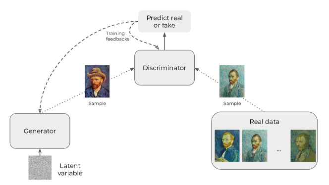
Figure 1: Illustration of the original GAN model. During the training phase, real data and generated data are fed to the discriminator (dotted arrows) which in turn must predict which data is real and which is fake. Feedback (in the form of gradients of the loss) are then sent to the generator and the discriminator (broken arrows) based on predictions from the latter to update their parameters (through back-propagation in the case of neural networks). Note that the generator does not directly have access to real data.

Since GANs initially emerged from the deep learning community, the first line of work primarily relied on empirical insights and general mathematical intuitions. Later on, a parallel line of work tackled the GAN problem from the statistical perspectives (Biau et al., 2020b, a; Chen et al., 2020; Liang, 2018; Singh et al., 2018; Luise et al., 2020; Uppal et al., 2019) as well as optimization and algorithmic viewpoints (Liang and Stokes, 2019; Kodali et al., 2017; Pfau and Vinyals, 2016; Nie and Patel, 2020; Nagarajan and Kolter, 2017; Genevay et al., 2018, 2019).

From a statistical perspective, the usual goal is to obtain a bound on the discrepancy between the learned distribution $P_{\textup{learner}}$ and the true distribution of the data $P^{*}=P_{\textup{user}}$ with respect to a given evaluation metric ${\sf d}$. A particularly relevant task is the quantification of the rate of convergence to zero of this discrepancy as the sample size $n$ grows to infinity. Given a family of candidate distributions $\mathcal{P}$, typical bounds are of the form

$$\mathbf{E}_{(X_{1},\dots,X_{n})\sim P_{\textup{obs}}}\big{[}{\sf d}(P_{\textup{learner}},P_{\textup{user}})\big{]}-\inf_{P\in\mathcal{P}}{\sf d}(P,P_{\textup{user}})\lesssim n^{-r(\alpha,\beta,d,D)}.$$ (3)

for some exponent $r(\alpha,\beta,d,D)>0$, where the parameter $\alpha$ characterises the complexity of the discriminator (e.g., the smoothness of the class $\mathcal{F}$ used in the IPM), $\beta$ represents the smoothness of the generator, $d$ is the intrinsic dimension of the data, (i.e., the dimension of the latent variable $\boldsymbol{U}$) and $D$ is the ambient dimension (e.g., the number of pixels in an image). Since $D$ is typically much larger than $d$, it is suitable to avoid any dependence on $D$ in the exponent $r(\alpha,\beta,d,D)$.

Chen et al. (2020); Liang (2018); Singh et al. (2018); Uppal et al. (2019) obtained rates depending on the smoothness of the density of the target distribution and (eventually) on the smoothness of the class $\mathcal{F}$ of admissible discriminators. Their rates do depend on the ambient dimension $D$, leading to the curse of dimensionality phenomenon; they do not account for possible low-dimensionnality of the data. Moreover, the learner distributions proposed in those papers are not necessarily easy-to-sample-from.

Without any smoothness assumptions, Biau et al. (2020a) provide large sample properties of the estimated distribution assuming that all the densities induced by the class of generators are dominated by a fixed known measure on a Borel subset of $\mathbb{R}^{D}$. When the admissible discriminators are neural networks with a given architecture, Biau et al. (2020b) obtained the parametric rate $n^{-1/2}$.

To our knowledge, Luise et al. (2020) is the only work which establishes statistical guarantees under the assumption that the data generating process is a smooth transformation of a low-dimensional latent distribution. Two key differences with our work is that Luise et al. (2020) measure quality of sampling through the Sinkhorn divergence (while we consider IPMs) and consider smoothness larger than $d/2$. The latter leads to parametric rates of convergence $n^{-1/2}$. Note also that the Sinkhorn divergence, introduced as a compelling computational alternative to the Wasserstein distance (Cuturi, 2013), does not admit a straightforward interpretation as a sampling error.

In this work, we assess the impact of the smoothness of the data generating process and the low-dimensionality of the latent space on the rates of convergence. The rates in the literature either depend on the ambient dimension, which can not explain the effectiveness of GANs, or assume strong smoothness assumption leading to parametric rate. This prevents a fine-grained analysis of the interplay between dimensions and smoothness. In this work we obtain rates which, in terms of dimension, depend only on the intrinsic dimension $d$ of the data and on the smoothness of the data generating process and the admissible discriminators.

3 Problem statement

We are given $n$ points $\boldsymbol{X}_{1},\dots,\boldsymbol{X}_{n}$ in $\mathbb{R}^{D}$, that we assume drawn independently from an unknown joint probability distribution $P_{\textup{obs}}^{(n)}$. We will make the hypothesis that the data points lie—up to a small noise—on a $d$-dimensional smooth manifold $\mathcal{M}$ with an intrinsic dimension $d$ much smaller than the ambient dimension $D$. More precisely, we assume that the $\boldsymbol{X}_{i}$’s are perturbed versions of $n$ independent copies of a point randomly sampled from a distribution $P^{*}$ supported on the smooth manifold $\mathcal{M}$. The goal of generative modeling is to design a smooth function

$$g:\mathbb{[}0,1]^{d}\to[0,1]^{D}$$ (4)

such that the image of the uniform distribution $\mathcal{U}_{d}:=\mathcal{U}([0,1]^{d})$ by $g$ is close to the target distribution $P^{*}$. Of course, this framework requires to make precise what is meant by “smoothness” of the function $g$ and how the closeness of two distributions is measured. Since the goal of the present work is to gain a better theoretical understanding of the problem of generative modeling, we assume that the ”intrinsic dimension” $d$ is known.

The following condition will be assumed to be true throughout this work, where $\sigma\geq 0$ and $\varepsilon\in[0,1]$ are fixed yet possibly unknown constants.

AssAAssumption A: There exists a mapping $g^{*}:[0,1]^{d}\rightarrow[0,1]^{D}$ (with $d\ll D$), as well as random vectors $\boldsymbol{U}_{1},\ldots,\boldsymbol{U}_{n}\in\mathbb{R}^{d}$ and $\boldsymbol{\xi}_{1},\ldots,\boldsymbol{\xi}_{n}\in\mathbb{R}^{D}$ such that

• $\boldsymbol{U}_{i}$ are iid uniformly distributed in the hypercube $[0,1]^{d}$ (denoted by $\boldsymbol{U}_{i}\stackrel{{\scriptstyle\textup{\rm iid}}}{{\sim}}\mathcal{U}_{d}$),

• $\max_{i=1,\ldots,n}\mathbf{E}[\|\boldsymbol{\xi}_{i}\|_{2}]\leq\sigma$ for some $\sigma<\infty$,

• For some $\mathcal{I}\subset\{1,\ldots,n\}$ of cardinality at least $(1-\varepsilon)n$, we have $\boldsymbol{X}_{i}=g^{*}(\boldsymbol{U}_{i})+\boldsymbol{\xi}_{i}$ for every $i\in\mathcal{I}$.

The parameters $\sigma$ and $\varepsilon$, referred to as the noise magnitude and the rate of contamination, are unknown but assumed to be small. The subset $\mathcal{I}$ in the last item of the assumption is the set of inliers. AssAAssumption A means that up to some noise, the inliers are drawn from the uniform distribution on the hyper-cube and pushed-forward by $g^{*}$. The setting considered here is adversarial: the set of inliers and the values of the outliers $\{\boldsymbol{X}_{i}:i\not\in\mathcal{I}\}$ may depend on all the random variables $\boldsymbol{U}_{i},\boldsymbol{X}_{i},\boldsymbol{\xi}_{i}$. Furthermore, $\boldsymbol{U}_{i}$ and $\boldsymbol{\xi}_{i}$ are not necessarily independent.

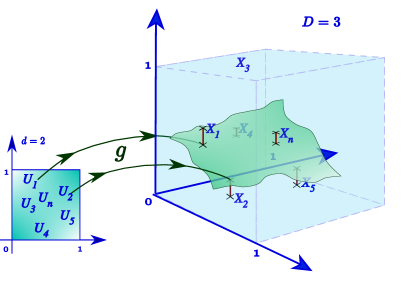
Figure 2: An illustration of Assumption A. Most $\boldsymbol{X}_{i}$’s are close to the manifold defined as the image of $[0,1]^{d}$ by the smooth map $g$. A small fraction of the $\boldsymbol{X}_{i}$’s (such as $\boldsymbol{X}_{3}$ in this figure) might be at a large distance from $g([0,1]^{d})$.

In what follows, we set $P^{*}=g^{*}\sharp\,\mathcal{U}_{d}$ and call it the oracle generator. Let ${\sf d}$ be a pseudo-metric on the space of all probability measures on $\mathbb{R}^{D}$. Most relevant examples in the present context are IPMs, but one could also consider the Wasserstein $q$-distances with $q\geq 1$, the Hellinger distance, the maximum mean discrepancy and so on. For every candidate generator $g$—a measurable mapping from $[0,1]^{d}$ to $\mathbb{R}^{D}$—we define the risk

$$R_{{\sf d},P^{*}}(g)\coloneqq{\sf d}\big{(}g\sharp\,\mathcal{U}_{d},P^{*}\big{)}.$$ (5)

Our goal is to find a mapping

$$\widehat{G}:(\mathbb{R}^{D})^{n} \to\mathcal{G}$$ (6)

$$(\boldsymbol{X}_{1},\dots,\boldsymbol{X}_{n}) \mapsto\widehat{g}_{n},$$ (7)

such that $R_{{\sf d},P^{*}}(\widehat{g}_{n})$ is as small as possible. Note here that $R_{{\sf d},P^{*}}(\widehat{g}_{n})$ is a random variable, since $\widehat{g}_{n}$ is random. Let $\mathcal{G}$ be a set of smooth (at least Lipschitz continuous) functions from $[0,1]^{d}$ to $\mathbb{R}^{D}$. We define the generator minimizing the empirical risk, hereafter referred to as the ERM, by

$$\widehat{g}_{n,\mathcal{G}}^{\textup{ERM}}\in\text{arg}\min_{g\in\mathcal{G}}{\sf d}\big{(}g{\sharp}\,\mathcal{U}_{d},\widehat{P}_{n}\big{)}.$$ (ERM)

We assume that the minimum is attained. Our results extend easily to the case in which it is not attained but adds some unnecessary technicalities. Our main result, presented in the next section, provides an upper bound on the risk (5) of the ERM.

To enforce requirement R2R2, we consider distances on the space of probability distributions that can be expressed as integral probability metrics for a class $\mathcal{F}$ of real-valued functions defined on $[0,1]^{D}$. More precisely, we define an integral probability metrics (IPM) for $\mathcal{F}$ as follows:

$${\sf d}_{\mathcal{F}}(P,Q)=\sup_{f\in\mathcal{F}}\lvert\mathbf{E}_{P}[f(\boldsymbol{X})]-\mathbf{E}_{Q}[f(\boldsymbol{X})]\rvert.$$ (8)

Classical examples are the total variation and the Wasserstein-1 distances, corresponding respectively to $\mathcal{F}=\{f:\sup_{x}|f(x)|\leq 1\}$ and $\mathcal{F}=\{f:|f(x)-f(y)|\leq\|x-y\|\text{ for all }x,y\}$.

4 Warming up: guarantees in the noiseless setting for ${\mathsf{W}}_{1}$W1

Let us first consider the noiseless and uncontaminated setting $\sigma=\varepsilon=0$, corresponding to $P_{\textup{obs}}=(P^{*})^{\otimes n}$. To convey the main ideas of this work without diving into technicalities, we first consider the case of the Wasserstein ${\mathsf{W}}_{1}$-distance. Using arguments that are now standard in learning theory, we get

$$R_{{\sf d},P^{*}}(\widehat{g}_{n,\mathcal{G}}^{\textup{ERM}})\leq\inf_{g\in\mathcal{G}}{\sf d}\big{(}g{\sharp}\,\mathcal{U}_{d},P^{*}\big{)}+2\,{\sf d}\big{(}\widehat{P}_{n},P^{*}\big{)}.$$ (9)

This inequality holds for any pseudo-metric $d$. It follows from the following chain of inequalities:

$$R_{{\sf d},P^{*}}(\widehat{g}_{n,\mathcal{G}}^{\textup{ ERM}}) ={\sf d}\big{(}\widehat{g}_{n,\mathcal{G}}^{\textup{ERM}}\sharp\,\mathcal{U}_{d},P^{*}\big{)}$$ (10)

$$\leq{\sf d}\big{(}\widehat{g}_{n,\mathcal{G}}^{\textup{ERM}}\sharp\,\mathcal{U}_{d},\widehat{P}_{n}\big{)}+{\sf d}\big{(}\widehat{P}_{n},P^{*}\big{)}$$ (11)

$$\leq\inf_{g\in\mathcal{G}}{\sf d}\big{(}g\sharp\,\mathcal{U}_{d},\widehat{P}_{n}\big{)}+{\sf d}\big{(}\widehat{P}_{n},P^{*}\big{)}$$ (12)

$$\leq\inf_{g\in\mathcal{G}}{\sf d}\big{(}g\sharp\,\mathcal{U}_{d},P^{*}\big{)}+2\,{\sf d}\big{(}\widehat{P}_{n},P^{*}\big{)}.$$ (13)

Note that if we replace in (ERM) the empirical distribution $\widehat{P}_{n}$ by another estimator $\tilde{P}_{n}$ of $P^{*}$, then (9) continues to be true with $\tilde{P}_{n}$ instead of $\widehat{P}_{n}$ in the right hand side.

The inequality (9) provides an upper bound on the risk that is composed of the approximation error $\inf_{g\in\mathcal{G}}{\sf d}\big{(}g\sharp\,\mathcal{U}_{d},P^{*}\big{)}$ and the stochastic error $2\,{\sf d}\big{(}\widehat{P}_{n},P^{*}\big{)}$. While the former is unavoidable, it is not clear how tight the latter is. In particular, the fact that the term $2\,{\sf d}\big{(}\widehat{P}_{n},P^{*}\big{)}$ measures the distance between the unknown distribution $P^{*}$ and an approximation of it that does not take into account the specific structure of $P^{*}$ suggests that it might be possible to get a better upper bound.

This being said, we stick here to inequality (9) and devote the rest of this paper to establishing upper bounds on the stochastic error. To this end, we take advantage of the interplay between the assumptions on $P_{X}$ and $P^{*}$ on the one hand, and the set $\mathcal{F}$ defining the IPM ${\sf d}={\sf d}_{\mathcal{F}}$ on the other hand. In the case when both the mapping $g^{*}$ underlying $P^{*}$ and the elements of $\mathcal{F}$ are Lipschitz, we get the following result.

Theorem 4.1.

Let AssAAssumption A be fulfilled with $\sigma=\varepsilon=0$ and $g^{*}\in\textup{Lip}_{L}([0,1]^{d})$ for some $L>0$. Let ${\sf d}=\mathsf{W}_{1}$ and set $\widehat{g}_{n}=\widehat{g}_{n,\mathcal{G}}^{\textup{ ERM}}$. Then, for some universal constant $c>0$,

$$\mathbf{E}[R_{{\mathsf{W}}_{1},P^{*}}(\widehat{g}_{n})]\leq\inf_{g\in\mathcal{G}}R_{{\mathsf{W}}_{1},P^{*}}(g)+\frac{cL\sqrt{d}}{n^{1/d}\wedge n^{1/2}}\big{(}1+\mathds{1}_{d=2}\log n\big{)}.$$ (14)

The full proof of this result being postponed to Section 7.1, we provide here a sketch of it. In view of (9), it suffices to upper bound ${\sf d}(\widehat{P}_{n},P)={\mathsf{W}}_{1}(\widehat{P}_{n},P^{*})$. Since $P^{*}$ and $\widehat{P}_{n}$ are the pushforward measures of $\mathcal{U}_{d}$ and its empirical counterpart by the same Lipschitz mapping, and the composition of two Lipschitz mappings is still Lipschitz, we can upper bound ${\mathsf{W}}_{1}(\widehat{P}_{n},P^{*})$ by $L{\mathsf{W}}_{1}(\widehat{P}_{U,n},\mathcal{U}_{d})$. Here, $\widehat{P}_{U,n}$ is the empirical distribution of $\boldsymbol{U}_{1},\ldots,\boldsymbol{U}_{n}$ independently sampled from $\mathcal{U}_{d}$. It is known that, for the Wasserstein-1 distance, there is a universal constant $c>0$ such that $\mathbf{E}[{\mathsf{W}}_{1}(\widehat{P}_{U,n},\mathcal{U}_{d})]$ is upper bounded by the second summand of the right hand side of (14); this fact has been established in the seminal paper Dudley (1969) and later refined and extended by many authors; see Weed and Bach (2019); Singh and Póczos (2018); Lei (2020) and references therein. The version we use here (with an explicit dependence of the constant on the dimension) can be found in Niles-Weed and Rigollet (2019, Prop. 1). This completes the proof.

Some remarks are in order. First, the rate of convergence to zero of the stochastic term, when the sample size goes to infinity, is characterized by the intrinsic dimension only. This rate, $n^{-1/d}$, is much smaller than the naive rate $n^{-1/D}$ provided that the intrinsic dimension is small as compared to $D$. To the best of our knowledge, despite the embarrassing simplicity of this result, this is the first time that this phenomenon is highlighted in the context of generative modeling.

The second remark concerns the fact that the choice of the set $\mathcal{G}$ in (ERM) impacts only the first term, the approximation error, in the risk bound given by (14). This indicates that inequality (14) might not be tight when $\mathcal{G}$ is a very narrow set. On the positive side, this bound implies that the set $\mathcal{G}$ can be chosen very large, as long as feature R1R1 holds and optimisation problem (ERM) is computationally tractable. Finally, one can wonder whether the assumption that $g^{*}$ is Lipschitz is realistic in some applications. We believe that it is. Indeed, the generator learned by GAN is a Lipschitz function of the input (Seddik et al., 2020) and leads to qualitatively good results. Therefore, it makes perfect sense to assume that $g^{*}$ is Lipschitz.

5 Main result in the noisy setting for smoothness classes

The rate of convergence obtained in the previous section might be overly pessimistic. Indeed, the Wasserstein distance ${\mathsf{W}}_{1}$ might be very weak for many applications: it may be sufficient to take as $\mathcal{F}$ a set which is much smaller than that of the Lipschitz functions. In particular, one can consider the case where $\mathcal{F}$ is a smoothness class with a degree of smoothness strictly larger than one. The main result stated below considers this setting and answers the following three questions:

• Can we take advantage of the further smoothness of $g^{*}$ and that of the functions in $\mathcal{F}$ for improving the risk bound (14)?

• How does the noise magnitude $\sigma$ impact the risk?

• Can we get meaningful risk bounds if some data points $\boldsymbol{X}_{i}$ are corrupted?

To answer these questions, we consider the case of smoothness classes containing all the functions with bounded partial derivatives up to a given order. Let $\mathcal{X}\subset\mathbb{R}^{D}$ be some compact set, which will be chosen to be $[0,1]^{D}$ later on in this section. In what follows, for every positive integer $\alpha$, $C^{\alpha}(\mathcal{X},\mathbb{R})$ denotes the set of all $\alpha$-times continuously differentiable functions. In addition, for a multi-index $\boldsymbol{k}\in\mathbb{N}^{D}$, we write $\texttt{D}^{\boldsymbol{k}}f$ for the $\boldsymbol{k}$-th order differential of $f$. Define the $\alpha$-smoothness class $\mathcal{W}^{\alpha}(\mathcal{X};r)$ over $\mathcal{X}$ with radius $L>0$ by

$$\mathcal{W}^{\alpha}(\mathcal{X};L)\coloneqq\bigg{\{}f\in C^{\alpha}(\mathcal{X},\mathbb{R}):\max_{\lvert\boldsymbol{k}\rvert\leq\alpha}\ \lVert\texttt{D}^{\boldsymbol{k}}f\rVert_{\infty}\leq L\bigg{\}}.$$ (15)

Clearly, $\mathcal{W}^{1}(\mathcal{X};L)$ is included in the set $\text{Lip}_{L}(\mathcal{X})$ of Lipschitz-continuous functions. Furthermore, one can check that $\mathcal{W}^{1}(\mathcal{X};L)$ is dense in $\text{Lip}_{L}(\mathcal{X})$.

Theorem 5.1.

Let AssAAssumption A hold and let the coordinates $g_{j}^{*}$ of $g^{*}$ belong to $\mathcal{W}^{\alpha}([0,1]^{d},L)$ for some $L\geq 1$. Then, if $\mathcal{F}=\mathcal{W}^{\alpha}([0,1]^{D},1)$ in the definition of the IPM, we have

$$\mathbf{E}[R_{{\sf d}_{\mathcal{F}},P^{*}}(\widehat{g}_{n,\mathcal{G}}^{\textup{ERM}})]\leq\inf_{g\in\mathcal{G}}R_{{\sf d}_{\mathcal{F}},P^{*}}(g)+L(\sigma+2\varepsilon)+\frac{cL^{\alpha}}{n^{\alpha/d}\wedge n^{1/2}}\big{(}1+\mathds{1}_{d=2\alpha}\log n\big{)}.$$ (16)

where $c$ is a constant which depends only on $\alpha,d,D$.

Let us note that this theorem answers the three questions Q1Q1-Q3Q3. In particular, it shows that if the oracle generator map $g^{*}$ is $\alpha$-smooth with $\alpha\leq d/2$, and the test function defining the distance ${\sf d}_{\mathcal{F}}$ are $\alpha$-smooth as well, then the last term of the risk bound of the generator minimizing the empirical risk is of order $n^{-\alpha/d}$. This rate improves with increasing $\alpha$ and reaches the optimal rate $n^{-1/2}$, up to a log factor, when $\alpha=d/2$. It also follows from (16) that the risk of the generator $\widehat{g}_{n,\mathcal{G}}^{\textup{ERM}}$ decreases linearly fast in the noise magnitude $\sigma$ and the contamination rate $\varepsilon$, when these parameters go to zero.

As mentioned earlier, (16) is a consequence of (9) and we do not know whether the latter is tight. However, we can show that the right hand side of (16) is a tight upper bound on the right hand side of (16). More precisely, as stated in the next result, the dependence on $\sigma$ and $\varepsilon$ is tight, while the dependence on $n$ is tight when $\alpha=1$ or $\alpha>d/2$.

Theorem 5.2.

Let $\mathcal{P}_{n,D}(d,\sigma,\varepsilon,g^{*})$ be the set of all distributions of $n$ points $(\boldsymbol{X}_{1},\ldots,\boldsymbol{X}_{n})$ in $\mathbb{R}^{D}$ satisfying AssAAssumption A. Let $\mathcal{G}^{*}$ be a set of functions $g:[0,1]^{d}\to[0,1]^{D}$ containing the linear functions. If $\sigma\leq 1/2$ and $\mathcal{F}$ contains the projection onto the first axis $\boldsymbol{x}\in[0,1]^{D}\mapsto x_{1}\in\mathbb{R}$, then there is a universal constant $c_{1}>0$ such that

$$\sup_{g^{*}\in\mathcal{G}^{*}}\sup_{P^{(n)}\in\mathcal{P}_{n,D}(d,\sigma,\varepsilon,g^{*})}\mathbf{E}_{P^{(n)}}[\mathsf{d}_{\mathcal{F}}(\widehat{P}_{n},P^{*})]\geq c_{1}\Big{(}\sigma+\varepsilon+\frac{1}{n^{1/2}}\Big{)}.$$ (17)

If, in addition, $\mathcal{F}$ contains the set of all $1$-Lipschitz functions, then

$$\sup_{g^{*}\in\mathcal{G}^{*}}\sup_{P^{(n)}\in\mathcal{P}_{n,D}(d,\sigma,\varepsilon)}\mathbf{E}_{\mathcal{P}^{(n)}}[\mathsf{d}_{\mathcal{F}}(\widehat{P}_{n},P^{*})]\geq c_{1}(\sigma+\varepsilon)+\frac{c_{d}\big{(}1+\mathds{1}_{d=2}\log n\big{)}}{n^{1/d}\wedge n^{1/2}},$$ (18)

where $c_{1}$ is a universal constant and $c_{d}$ is a constant depending on $d$.

The proof of the theorem is postponed to Section 7.4. Note that it does not establish the tightness of the dependence of the bound in $n$ in the case of smoothness $\alpha\in(1,d/2)$. However, it is very likely that the rate is also optimal in this case as well.

To complete this section, we show that the dependence in $\varepsilon$ and $\sigma$ of the upper bound (16) is tight.

Theorem 5.3.

Let $\mathcal{P}_{n,D}(d,\sigma,\varepsilon,g^{*})$ be the set of all distributions of $n$ points $(\boldsymbol{X}_{1},\ldots,\boldsymbol{X}_{n})$ in $\mathbb{R}^{D}$ satisfying AssAAssumption A. Let $\mathcal{G}^{*}$ be a set of functions $g:[0,1]^{d}\to[0,1]^{D}$ containing the affine functions. Assume that $\mathcal{F}$ is a set of functions $f:[0,1]^{D}\to\mathbb{R}$ bounded by $L$ and containing the projection onto the first axis $\boldsymbol{x}\in[0,1]^{D}\mapsto x_{1}\in\mathbb{R}$. Then, if $\sigma\leq 1/2$ and $n\geq(6/\varepsilon)\log(20L/\varepsilon)$, we have

$$\inf_{\widehat{g}_{n}}\ \sup_{g^{*}\in\mathcal{G}^{*}}\sup_{P^{(n)}\in\mathcal{P}_{n,D}(d,\sigma,\varepsilon,g^{*})}\mathbf{E}[R_{{\sf d}_{\mathcal{F}},P^{*}}(\widehat{g}_{n})]\geq 0.1(\sigma+\varepsilon),$$ (19)

where the inf is taken over all possible generators $\widehat{g}_{n}$.

The proof of this result is postponed to Section 7.5. If we compare this lower bound with the upper bound of Theorem 5.1, we see that the linear dependence of the expected risk on the parameters $\sigma$ and $\varepsilon$ is optimal and cannot be improved. This is true for any generator, meaning that the empirical risk minimizer is minimax rate-optimal in terms of $\sigma$ and $\varepsilon$. We are currently working on establishing similar lower bounds showing the optimality in terms of $n$ as well.

6 Conclusion and outlook

In this work, we introduced a general and nonparametric framework for learning generative models. Given data in a possibly high-dimensional space, we learn their distribution in order to sample new data points that resemble the training ones, while not being identical to those. A key point in our work is to leverage the fact that the distribution of the training samples, up to some noise and adversarial contamination, is supported by a low-dimensional smooth manifold. This allows us to alleviate the curse of dimensionality. Such an assumption is very reasonable as it reflects the structural properties of the training samples. For instance, the MNIST dataset (LeCun, 1998) is composed of $28\times 28$ pixels pictures of handwritten digits while the intrinsic dimension of the data is estimated to be around $14$ (Costa and Hero, 2004; Levina and Bickel, 2005).

We established risk bounds for the minimizer of the distance between the empirical distribution and admissible generators, where an admissible generator is a smooth function pushing forward a low-dimensional uniform distribution into the high-dimensional sample space. We use Integral Probability Metrics for measuring the discrepancy between the target distribution and our estimate: These metrics, which include the total variation and the Wasserstein-1 distances, mimic the role of a discriminator which would try to discriminate between true samples and the simulated ones.

By proving new bounds on the distance between such distributions and their empirical counterparts, we were able to derive nonasymptotic bounds for the regret of our empirical risk minimizer, with rates of convergence that only depend on the ambient dimension through fixed multiplicative constants. Our new bounds, which are of independent interest, leverage both the smoothness of the distribution of the samples and that of the functions in the IPM class.

We were also able to take into account possible adversarial corruption of the training samples both by noise (e.g., blurry images) and by a small proportion of outliers (i.e., wrong samples in the training set), inducing some error terms that are shown to be unavoidable. To the best of our knowledge, this is the first result assessing the influence of the noise and of the contamination on the error of generative modeling. This constitutes an appealing complement to the recently obtained statistical guarantees (Biau et al., 2020b; Luise et al., 2020).

As a route for future work, we believe that our regret bounds are not minimax optimal in all possible regimes (depending on the smoothness of the generators). Namely, it is not clear that fitting our generator to the empirical distribution $\widehat{P}_{n}$ yields an optimal method, especially when the smoothness $\alpha$ is less than the half of the dimension $d$. It might be more judicious to fit the generator to a smoothed version of the empirical distribution $\widehat{P}_{n}$.

7 Proofs

This section contains the proofs of the main results stated in previous sections. We start by providing the proof of Theorem 4.1. Then, the proof of Theorem 5.1 is presented up to the proof of a technical lemma on the composition of smooth functions, postponed to Section 7.3.

7.1 Proof of Theorem 4.1Theorem 1

To ease notation, we write $\widehat{g}_{n}$ instead of $\widehat{g}_{n,\mathcal{G}}^{\textup{ERM}}$. In view of (9), we have

$$R_{{\mathsf{W}}_{1},P^{*}}(\widehat{g}_{n})\leq\inf_{g\in\mathcal{G}}{\mathsf{W}}_{1}(g\sharp\,\mathcal{U}_{d},P^{*})+2{\mathsf{W}}_{1}(\widehat{P}_{n},P^{*}).$$ (20)

Using the variational formulation of the Wasserstein-1 distance we write

$${\mathsf{W}}_{1}(\widehat{P}_{n},P^{*}) =\sup_{f\in\textup{Lip}_{1}([0,1]^{D})}\Big{|}\frac{1}{n}\sum_{i=1}^{n}f(\boldsymbol{X}_{i})-\mathbf{E}_{\boldsymbol{X}\sim P^{*}}f(\boldsymbol{X})\Big{|}$$ (21)

$$=\sup_{f\in\textup{Lip}_{1}([0,1]^{D})}\Big{|}\frac{1}{n}\sum_{i=1}^{n}f\circ g^{*}(\boldsymbol{U}_{i})-\mathbf{E}_{{\boldsymbol{U}}\sim\mathcal{U}_{d}}f\circ g^{*}(\boldsymbol{U})\Big{|}$$ (22)

$$=\sup_{h\in\mathcal{H}_{L}}\Big{(}\frac{1}{n}\sum_{i=1}^{n}h(\boldsymbol{U}_{i})-\mathbf{E}_{{\boldsymbol{U}}\sim\mathcal{U}_{d}}h(\boldsymbol{U})\Big{)}$$ (23)

where we define the class $\mathcal{H}_{L}=\{h:[0,1]^{d}\to\mathbb{R}:h=f\circ g^{*},f\in\textup{Lip}_{1}([0,1]^{D})\}$. Finally, taking the expectation and noting that $\mathcal{H}_{L}$ is a subset of the the $L$-Lipschitz functions on $[0,1]^{d}$ with values in $\mathbb{R}$, we get

$$\mathbf{E}[{\mathsf{W}}_{1}(\widehat{P}_{n},P^{*})] \leq\mathbf{E}\bigg{[}\sup_{h\in\textup{Lip}_{L}([0,1]^{d})}\Big{(}\frac{1}{n}\sum_{i=1}^{n}h(\boldsymbol{U}_{i})-\mathbf{E}_{{\boldsymbol{U}}\sim\mathcal{U}_{d}}h(\boldsymbol{U})\Big{)}\bigg{]}$$ (24)

$$\leq L\,\mathbf{E}[{\mathsf{W}}_{1}(\widehat{P}_{U,n},\mathcal{U}_{d})]$$ (25)

$$\leq\frac{cL\sqrt{d}}{n^{1/d}\wedge n^{1/2}}\big{(}1+\mathds{1}_{d=2}\log n\big{)},$$ (26)

with $c$ a universal constant. The last inequality follows from Niles-Weed and Rigollet (2019, Proposition 1).

7.2 Proof of Theorem 5.1Theorem 2

In view of (9), we need to establish an upper bound on the expected stochastic error

$$\textup{NoisyStochErr}_{n}=\mathbf{E}[{\sf d}_{\mathcal{F}}(P_{n},P^{*})]=\mathbf{E}\bigg{[}\sup_{f\in\mathcal{F}}\bigg{|}\frac{1}{n}\sum_{i=1}^{n}f(\boldsymbol{X}_{i})-\mathbf{E}[f(g^{*}(\boldsymbol{U}))]\bigg{|}\bigg{]},$$ (27)

where $\boldsymbol{U}\sim\mathcal{U}_{d}$ and $\mathcal{F}=\mathcal{W}^{\alpha}([0,1]^{D},1)$. The first step in the proof is a lemma showing the influence of the noise and the corruption on the error $\textup{StochErr}_{n}$.

Lemma 1.

If $P_{X}$ satisfies AssAAssumption A with $\varepsilon\in[0,1]$ and all the functions in $\mathcal{F}$ are bounded by a constant $L_{\mathcal{F}}$ and Lipschitz with constant $L_{\mathcal{F}}$, then

$$\textup{NoisyStochErr}_{n}\leq L_{\mathcal{F}}\sigma+2M_{\mathcal{F}}\varepsilon+\textup{NoiseFreeStochErr}_{n},$$ (28)

where

$$\textup{NoiseFreeStochErr}_{n}=\mathbf{E}\bigg{[}\sup_{f\in\mathcal{F}}\bigg{|}\frac{1}{n}\sum_{i=1}^{n}(f\circ g^{*})(\boldsymbol{U}_{i})-\mathbf{E}[(f\circ g^{*})(\boldsymbol{U})]\bigg{|}\bigg{]},$$ (29)

with $\boldsymbol{U},\boldsymbol{U}_{1},\ldots,\boldsymbol{U}_{n}$ iid random vectors drawn from $\mathcal{U}_{d}$.

Proof 7.1.

The triangle inequality yields

$$\textup{StochErr}_{n}\leq\mathbf{E}\bigg{[}\sup_{f\in\mathcal{F}}\bigg{|}\frac{1}{n}\sum_{i=1}^{n}\big{\{}f(\boldsymbol{X}_{i})-(f\circ g^{*})(\boldsymbol{U}_{i})\big{\}}\bigg{|}\bigg{]}+\textup{NoiseFreeStochErr}_{n}.$$ (30)

Let us define $\boldsymbol{Y}_{i}=g^{*}(\boldsymbol{U}_{i})+\boldsymbol{\xi}_{i}$ for $i=1,\ldots,n$. The third item of AssAAssumption A implies that $\boldsymbol{Y}_{i}=\boldsymbol{X}_{i}$ for $i\in\mathcal{I}$. For $i\not\in\mathcal{I}$, we have $|f(\boldsymbol{X}_{i})-f(\boldsymbol{Y}_{i})|\leq 2M_{\mathcal{F}}$. Therefore, the first term in the right hand side of the last display can be further bounded as follows:

$$\bigg{|}\frac{1}{n}\sum_{i=1}^{n}\big{\{}f(\boldsymbol{X}_{i})-(f\circ g^{*})(\boldsymbol{U}_{i})\big{\}}\bigg{|} \leq\bigg{|}\frac{1}{n}\sum_{i=1}^{n}\big{\{}f(\boldsymbol{Y}_{i})-(f\circ g^{*})(\boldsymbol{U}_{i})\big{\}}\bigg{|}+\frac{2M_{\mathcal{F}}(n-n_{\mathcal{I}})}{n}$$ (31)

$$\leq\frac{L_{\mathcal{F}}}{n}\sum_{i=1}^{n}\big{\|}\boldsymbol{Y}_{i}-g^{*}(\boldsymbol{U}_{i})\big{\|}+2M_{\mathcal{F}}\,\varepsilon$$ (32)

$$=\frac{L_{\mathcal{F}}}{n}\sum_{i=1}^{n}\big{\|}\boldsymbol{\xi}_{i}\big{\|}+2M_{\mathcal{F}}\,\varepsilon.$$ (33)

To get the claimed result, it suffices to take the expectation of both sides of the last display.

The next step consists in upper bounding the stochastic error in the noise free case. If we use the notation $\mathcal{F}\circ g^{*}=\{f\circ g^{*}:f\in\mathcal{F}\}$, the noise free stochastic error can be written as

$$\textup{NoiseFreeStochErr}_{n}=\mathbf{E}[{\sf d}_{\mathcal{F}\circ g^{*}}(\widehat{P}_{U,n},\mathcal{U}_{d})].$$ (34)

We see that the problem is reduced to that of evaluating the distance between the uniform distribution and the empirical distribution of $n$ independent random points uniformly distributed on the unit hypercube. In order to upper bound this distance, we first show that the class $\mathcal{F}\circ g^{*}$, under the assumptions of Theorem 5.1, is included in a smoothness class of order $\alpha$. The precise statement is the following.

Lemma 2.

Let $g:[0,1]^{d}\to[0,1]^{D}$ and $h:[0,1]^{D}\to[-1,1]$ two mappings such that $g\in\mathcal{W}^{\alpha}([0,1]^{d},L)$ and $h\in\mathcal{W}^{\alpha}([0,1]^{D},1)$ for some $\alpha\in\mathbb{N}^{*}$ and some $L\geq 1$. Then, there exists a constant $C=C(D,d,\alpha)$ such that

$$\lvert\textup{\tt D}^{\boldsymbol{k}}(h\circ g)(\boldsymbol{x})\rvert\leq CL^{\alpha},\quad\forall\boldsymbol{x}\in[0,1]^{d},$$ (35)

for every multi-index $\boldsymbol{k}=(k_{1},\dots,k_{d})\in\mathbb{N}^{d}$ such that $\lvert\boldsymbol{k}\rvert\leq\alpha$.

This lemma, in conjunction with (34) and the assumption $g^{*}\in\mathcal{W}^{\alpha}([0,1]^{d},L)$, implies that

$$\textup{NoiseFreeStochErr}_{n} \leq\mathbf{E}[{\sf d}_{\mathcal{W}^{\alpha}([0,1]^{d},CL^{\alpha})}(\widehat{P}_{U,n},\mathcal{U}_{d})]$$ (36)

$$=CL^{\alpha}\mathbf{E}[{\sf d}_{\mathcal{W}^{\alpha}([0,1]^{d},1)}(\widehat{P}_{U,n},\mathcal{U}_{d})].$$ (37)

The last step is to use Schreuder (2020, Theorem 4), which provides the inequality

$$\mathbf{E}[{\sf d}_{\mathcal{W}^{\alpha}([0,1]^{d},CL^{\alpha})}(\widehat{P}_{U,n},\mathcal{U}_{d})] \leq\tilde{C}L^{\alpha}n^{-(\alpha\wedge d/2)/d}(1+\mathds{1}_{\alpha=d/2}\log n).$$ (38)

This completes the proof of the theorem.

7.3 Image of a smoothness class by a smooth function

Proof of Lemma 2  The proof relies on Fraenkel (1978, Formula B) providing an explicit formula for derivatives of composite functions: for any multi-index $\boldsymbol{k}$ such that $1\leq\lvert\boldsymbol{k}\rvert\leq\alpha$ and for any $\boldsymbol{x}\in[0,1]^{d}$,

$$\textup{\tt D}^{\boldsymbol{k}}(h\circ g)(\boldsymbol{x})=\boldsymbol{k}!\sum_{\boldsymbol{a}:1\leq\lvert\boldsymbol{a}\rvert\leq\lvert\boldsymbol{k}\rvert}\frac{(\textup{\tt D}^{\boldsymbol{a}}h)(g(\boldsymbol{x}))}{\boldsymbol{a}!}Q_{\boldsymbol{k},\boldsymbol{a}}(g;\boldsymbol{x}),$$ (39)

where $Q_{\boldsymbol{k},\boldsymbol{a}}(g;\cdot)$ is a homogeneous polynomial of degree $\lvert\boldsymbol{a}\rvert$ in derivatives of $g_{1},\dots,g_{D}$. Since the partial derivatives of $h$ of any order up to $\alpha$ are bounded by one, we infer from the last display that

$$\big{|}\textup{\tt D}^{\boldsymbol{k}}(h\circ g)(\boldsymbol{x})\big{|}=\boldsymbol{k}!\sum_{\boldsymbol{a}:1\leq\lvert\boldsymbol{a}\rvert\leq\lvert\boldsymbol{k}\rvert}\frac{1}{\boldsymbol{a}!}\big{|}Q_{\boldsymbol{k},\boldsymbol{a}}(g;\boldsymbol{x})|.$$ (40)

We can give an explicit expression of $Q_{\boldsymbol{k},\boldsymbol{a}}$ using the following notation. Let $r$ be the cardinality of the set $\{\boldsymbol{\beta}\in\mathbb{N}^{d}\,|\,0<\boldsymbol{\beta}\leq\boldsymbol{\gamma}\}$ and $\boldsymbol{\beta}(1),\ldots,\boldsymbol{\beta}(r)$ be its elements somehow enumerated. Define, for $\boldsymbol{\gamma}\in\mathbb{N}^{d}$ and for $a\in\mathbb{N}$, the set of multi-indices

$$R(\boldsymbol{\gamma},a)=\bigg{\{}\boldsymbol{\rho}\in\mathbb{N}^{r}\,\big{|}\,\sum_{j=1}^{r}\rho_{j}\boldsymbol{\beta}(j)=\boldsymbol{\gamma},\lvert\boldsymbol{\rho}\rvert=a\bigg{\}},$$ (41)

and, for any $v:\mathbb{R}^{d}\to\mathbb{R}$, the polynomials

$$P_{\boldsymbol{\gamma}}(a,v;\boldsymbol{x})=\sum_{\boldsymbol{\rho}\in R(\gamma,a)}\frac{a!}{\boldsymbol{\rho}!}\prod_{j=1}^{r}\frac{(\textup{\tt D}^{\boldsymbol{\beta}(j)}v(\boldsymbol{x}))^{\rho_{j}}}{\boldsymbol{\beta}(j)!}.$$ (42)

The functions $Q_{\boldsymbol{k},\boldsymbol{a}}$ in (40) are given by

$$Q_{\boldsymbol{k},\boldsymbol{a}}(g;\boldsymbol{x})=\sum_{\boldsymbol{\gamma}(1)+\ldots+\boldsymbol{\gamma}(D)=\boldsymbol{k}}\prod_{m=1}^{D}P_{\boldsymbol{\gamma}(m)}({a}_{m},g_{m};\boldsymbol{x}).$$ (43)

Since, according to the conditions of the lemma, all the partial derivatives of $g$ appearing in (42) for $v=g_{m}$ are bounded by $L\geq 1$, we have

$$\big{\lvert}P_{\boldsymbol{\gamma}(m)}({a}_{m},g_{m};\boldsymbol{x})\big{\rvert}\leq\sum_{\boldsymbol{\rho}\in R(\boldsymbol{\gamma}(m),{a}_{m})}L^{|\boldsymbol{\rho}|}\frac{{a}_{m}!}{\boldsymbol{\rho}!}\prod_{j=1}^{r}\frac{1}{\boldsymbol{\beta}(j)!}.$$ (44)

Since $|\boldsymbol{\rho}|\leq{a}_{m}$ and $|\boldsymbol{a}|\leq|\boldsymbol{k}|\leq\alpha$, this leads to

$$\big{|}Q_{\boldsymbol{k},\boldsymbol{a}}(g;\boldsymbol{x})\big{|} \leq L^{\alpha}\boldsymbol{a}!\sum_{\boldsymbol{\gamma}(1)+\ldots+\boldsymbol{\gamma}(D)=\boldsymbol{k}}\prod_{m=1}^{D}\left(\sum_{\boldsymbol{\rho}\in R(\boldsymbol{\gamma}(m),{a}_{m})}\frac{1}{\boldsymbol{\rho}!}\prod_{j=1}^{r}\frac{1}{\boldsymbol{\beta}(j)!}\right).$$ (45)

Combining this inequality with (40), we arrive at

$$\lvert\textup{\tt D}^{\boldsymbol{k}}(h\circ g)(\boldsymbol{x})\rvert \leq L^{\alpha}\boldsymbol{k}!\sum_{1\leq\lvert\boldsymbol{a}\rvert\leq\lvert\boldsymbol{k}\rvert}\sum_{\boldsymbol{\gamma}(1)+\dots+\boldsymbol{\gamma}(D)=\boldsymbol{a}}\prod_{m=1}^{D}\left(\sum_{\boldsymbol{\rho}\in R(\boldsymbol{\gamma}(m),{a}_{m})}\frac{1}{\boldsymbol{\rho}!}\prod_{j=1}^{r}\frac{1}{\boldsymbol{\beta}(r)!}\right).$$ (46)

Denoting by $C(D,d,\alpha)$ the maximum of the right hand side over all multi-indices $\boldsymbol{k}$ such that $|\boldsymbol{k}|\leq\alpha$, we get the claim of the lemma. ∎

7.4 Proof of the lower bounds in Theorem 5.2Theorem 3

Since the bound we wish to prove does not depend on the dimension, we assume without loss of generality that $D=d$. First, we start by considering the case $\sigma+\varepsilon\geq 2/n^{1/2}$.

Let us define $g^{*}(\boldsymbol{x})=(2\boldsymbol{x}+1)/4$. This function is clearly $1$-Lipschitz. Let $\xi_{1}$ be a random variable drawn from the uniform in $[0,1]$ distribution. We define $P_{0}^{(n)}$ to be the distribution of i.i.d. vectors $\boldsymbol{X}_{1},\ldots,\boldsymbol{X}_{n}$ such that $\boldsymbol{X}_{i}\stackrel{{\scriptstyle\rm dist}}{{\sim}}g^{*}(\boldsymbol{U})+\sigma\xi_{1}$ for $i=1,\ldots,n\varepsilon$ and $\boldsymbol{X}_{i}=(1,\ldots,1)^{\top}$ for $i>n\varepsilon$. Then, it is clear that $P_{0}^{(n)}\in\mathcal{P}_{n,D}\big{(}d,\sigma,(1-\varepsilon)n\big{)}$ and

$$\mathbf{E}_{P_{0}^{(n)}}[\mathsf{d}_{\mathcal{F}}(\widehat{P}_{n},P^{*})] =\mathbf{E}_{P_{0}^{(n)}}\bigg{[}\sup_{f\in\mathcal{F}}\bigg{|}\frac{1}{n}\sum_{i=1}^{n}f(\boldsymbol{X}_{i})-\mathbf{E}[(f\circ g^{*})(\boldsymbol{U})]\bigg{|}\bigg{]}$$ (47)

$$\geq\mathbf{E}_{P_{0}^{(n)}}\bigg{[}\bigg{|}\frac{1}{n}\sum_{i=1}^{n}X_{i,1}-\mathbf{E}[g^{*}(\boldsymbol{U})_{1}]\bigg{|}\bigg{]}$$ (48)

$$=\mathbf{E}_{P_{0}^{(n)}}\bigg{[}\bigg{|}\frac{1}{n}\sum_{i=1}^{n}\big{(}X_{i,1}-\mathbf{E}[X_{i,1}]\big{)}+\varepsilon+0.5\sigma-\varepsilon\mathbf{E}[g^{*}(\boldsymbol{U})_{1}]\bigg{|}\bigg{]}$$ (49)

$$=\mathbf{E}_{P_{0}^{(n)}}\bigg{[}\bigg{|}\frac{1}{n}\sum_{i=1}^{n}\big{(}X_{i,1}-\mathbf{E}[X_{i,1}]\big{)}+0.5(\sigma+\varepsilon)\bigg{|}\bigg{]}.$$ (50)

The first inequality above follows by replacing the sup over $\cal F$ by the corresponding expression evaluated at the representer $f_{0}(\boldsymbol{x})=x_{1}$. The third line above follows from $\mathbf{E}[X_{i,1}]=\mathbf{E}[g^{*}(\boldsymbol{U})_{1}]+0.5\sigma$ if $i\leq n\varepsilon$ whereas $\mathbf{E}[X_{i,1}]=1$ if $i>n\varepsilon$. The last line is a consequence of $\mathbf{E}[g(\boldsymbol{U})_{1}]=0.5$. Combining the above lower bound with the triangle inequality, we arrive at

$$\mathbf{E}_{P_{0}^{(n)}}[\mathsf{d}_{\mathcal{F}}(\widehat{P}_{n},P^{*})] \geq 0.5(\sigma+\varepsilon)-\mathbf{E}_{P_{0}^{(n)}}\bigg{[}\bigg{|}\frac{1}{n}\sum_{i=1}^{n}\big{(}X_{i,1}-\mathbf{E}[X_{i,1}]\big{)}\bigg{|}\bigg{]}$$ (51)

$$\geq 0.5(\sigma+\varepsilon)-\bigg{(}\mathbf{E}_{P_{0}^{(n)}}\bigg{[}\bigg{|}\frac{1}{n}\sum_{i=1}^{n}\big{(}X_{i,1}-\mathbf{E}[X_{i,1}]\big{)}\bigg{|}^{2}\bigg{]}\bigg{)}^{1/2}$$ (52)

$$\geq 0.5(\sigma+\varepsilon)-0.5/\sqrt{n}$$ (53)

$$\geq\big{(}\sigma+\varepsilon+1/\sqrt{n}\big{)}/6.$$ (54)

To get the second line above, we used that the first-order moment is bounded by the second-order moment. In the third line, we used that the variance of the sum of independent random variables is the sum of variances and that the variance of a random variables taking its values in $[0,1]$ is always $\leq 1/4$. Finally, the last line is derived from the assumption $\sigma+\varepsilon\geq 2/\sqrt{n}$.

We now turn to the case $\sigma+\varepsilon\leq 2/\sqrt{n}$. In this case, we use the same distribution $P_{0}^{(n)}$ as in the previous case but we choose $\sigma=\varepsilon=0$. From (50) we derive that

$$\mathbf{E}_{P_{0}^{(n)}}\big{[}\mathsf{d}_{\mathcal{F}}(\widehat{P}_{n},P^{*})\big{]} \geq\mathbf{E}_{P_{0}^{(n)}}\bigg{[}\bigg{|}\frac{1}{n}\sum_{i=1}^{n}\big{(}X_{i,1}-\mathbf{E}[X_{i,1}]\big{)}\bigg{|}\bigg{]}$$ (55)

$$\geq 0.5\,\mathbf{E}_{U_{i}\stackrel{{\scriptstyle\rm iid}}{{\sim}}\mathcal{U}_{1}}\bigg{[}\bigg{|}\frac{1}{n}\sum_{i=1}^{n}(U_{i}-0.5)\bigg{|}\bigg{]}\geq 0.105/\sqrt{n}$$ (56)

In view of the assumption $\sigma+\varepsilon\leq 2/\sqrt{n}$, this leads to

$$\mathbf{E}_{P_{0}^{(n)}}\big{[}\mathsf{d}_{\mathcal{F}}(\widehat{P}_{n},P^{*})\big{]} \geq\mathbf{E}_{P_{0}^{(n)}}\bigg{[}\bigg{|}\frac{1}{n}\sum_{i=1}^{n}\big{(}X_{i,1}-\mathbf{E}[X_{i,1}]\big{)}\bigg{|}\bigg{]}$$ (57)

$$\geq 0.5\,\mathbf{E}_{U_{i}\stackrel{{\scriptstyle\rm iid}}{{\sim}}\mathcal{U}_{1}}\bigg{[}\bigg{|}\frac{1}{n}\sum_{i=1}^{n}(U_{i}-0.5)\bigg{|}\bigg{]}\geq 0.035(\sigma+\varepsilon+1/\sqrt{n}),$$ (58)

which completes the proof of the first inequality of the theorem. For the second inequality, it suffices to combine the first inequality with the lower bound established in the seminal paper Dudley (1969).

7.5 Proof of the lower bound in Theorem 5.3

We split the proof of Theorem 5.3 into two propositions: The first one shows the tightness of the dependence on the contamination rate whereas the second one establishes the tightness of the dependence on the noise-level.

Proposition 3 (Tightness wrt to the contamination rate).

Under the assumptions of Theorem 5.3,

$$\inf_{\widehat{g}_{n}}\sup_{g^{*}}\sup_{P^{(n)}\in\mathcal{P}_{n,D}(d,\sigma,\varepsilon,g^{*})}\mathbf{E}[R_{{\sf d}_{\mathcal{F}},P^{*}}(\widehat{g}_{n})]\geq\varepsilon/3.$$ (59)

Proof 7.2.

It can be easily checked that the supremum of the expected risk over $\mathcal{P}_{n,D}(d,\sigma,\varepsilon,g^{*})$ is always not smaller than the supremum of the same quantity over $\mathcal{P}_{n,1}(d,0,\varepsilon,g^{*})$. To ease notation, we write $\mathcal{P}_{n}(d,\varepsilon,g^{*})=\mathcal{P}_{n,1}(d,0,\varepsilon,g^{*})$ and also set $\mu=\mathcal{U}_{d}$.

Step 1: Reduction to Huber contamination model.

Note that the set of admissible data distributions $\mathcal{P}_{n,D}(d,\varepsilon,g^{*})$ comprises the data distributions from Huber’s deterministic contamination model (Bateni and Dalalyan, 2020, Section 2.2), namely data distributions such that a (deterministic) proportion $(1-\varepsilon)$ of the data is distributed according to a reference distribution $P^{*}$ while the remaining proportion $\varepsilon$ is independently drawn from another distribution $Q$. Therefore, denoting by $\mathcal{P}^{\rm HDC}_{n}(d,\varepsilon,g^{*})$ such distributions, it holds, for any estimator $\widehat{g}_{n}$ and generator $g^{*}$,

$$\sup_{P^{(n)}\in\mathcal{P}_{n}(d,\varepsilon,g^{*})}\mathbf{E}[R_{{\sf d}_{\mathcal{F}},P^{*}}(\widehat{g}_{n})] =\sup_{P^{(n)}\in\mathcal{P}_{n}(d,\varepsilon,g^{*})}\mathbf{E}[\mathsf{d}_{\mathcal{F}}(g^{*}\sharp\mu,\widehat{g}_{n}\sharp\mu)]$$ (60)

$$\geq\sup_{P^{(n)}\in\mathcal{P}^{\rm HDC}_{n}(d,\varepsilon,g^{*})}\mathbf{E}[\mathsf{d}_{\mathcal{F}}(g^{*}\sharp\mu,\widehat{g}_{n}\sharp\mu)].$$ (61)

Furthermore, let us denote by $\mathcal{P}^{\rm HC}_{D}(d,\varepsilon,g^{*})$ the set of data distributions such that there is a distribution $Q$ defined on the same space as a reference distribution $P^{*}=g^{*}\sharp\mu$ such that the observations $\boldsymbol{X}_{1},\dots,\boldsymbol{X}_{n}$ are independent and drawn from the mixture distribution $(1-\varepsilon)P^{*}+\varepsilon Q$. In view of $\sup_{g,g^{\prime}}d_{\mathcal{F}}(g\sharp\mu,g^{\prime}\sharp\mu)\leq L$ and (Bateni and Dalalyan, 2020, Proposition 1), for any estimator $\widehat{g}_{n}$ and generator $g^{*}$, we have

$$\sup_{P^{(n)}\in\mathcal{P}^{\rm HDC}_{n}(d,\varepsilon,g^{*})}\mathbf{E}[\mathsf{d}_{\mathcal{F}}(g^{*}\sharp\mu,\widehat{g}_{n}\sharp\mu)]\geq\sup_{P^{(n)}\in\mathcal{P}^{\rm HC}_{n}(d,\varepsilon/2,g^{*})}\mathbf{E}[\mathsf{d}_{\mathcal{F}}(g^{*}\sharp\mu,\widehat{g}_{n}\sharp\mu)]-e^{-n\varepsilon/6}L.$$ (62)

The second step consists in lower bounding the risk in the Huber contamination model using an argument based on two simple hypotheses.

Step 2: Construction of hypotheses.

Let us define the generators $g_{1}^{*},g_{2}^{*}:[0,1]^{d}\to[0,1]$ as

$$g_{1}^{*}(\boldsymbol{u})=(1-\varepsilon)u_{1}\quad\text{ and }\quad g_{2}^{*}(\boldsymbol{u})=(1-\varepsilon)u_{1}+\varepsilon,\quad\text{ for }\boldsymbol{u}=(u_{1},\dots,u_{d})\in[0,1]^{d}.$$ (63)

For contamination distributions $Q_{1}\coloneqq\mathcal{U}([1-\varepsilon,1])$ and $Q_{2}\coloneqq\mathcal{U}([0,\varepsilon])$, define the data generating distributions

$$P_{1}^{(n)}=[(1-\varepsilon)g^{*}_{1}\sharp\mu+\varepsilon Q_{1}]^{\otimes n}\text{ and }P_{2}^{(n)}=[(1-\varepsilon)g^{*}_{2}\sharp\mu+\varepsilon Q_{2}]^{\otimes n}.$$ (64)

One can easily check that $P_{1}^{(n)}=P_{2}^{(n)}=\mathcal{U}([0,1])^{\otimes n}$ and $P_{j}^{(n)}\in\mathcal{P}^{\rm HC}_{n}(d,\varepsilon,g_{j}^{*})$ for $j=1,2$. Using the fact that the maximum is larger than the arithmetic mean, in conjunction with the triangular inequality, we obtain

$$\sup_{g^{*}}\sup_{P^{(n)}\in\mathcal{P}^{\rm HC}_{n}(d,\varepsilon,g^{*})}\mathbf{E}[\mathsf{d}_{\mathcal{F}}(g^{*}\sharp\mu,\widehat{g}_{n}\sharp\mu)] \geq\frac{1}{2}\left[\mathbf{E}_{P_{1}^{(n)}}\mathsf{d}_{\mathcal{F}}(g_{1}^{*}\sharp\mu,\widehat{g}_{n}\sharp\mu)+\mathbf{E}_{P_{2}^{(n)}}\mathsf{d}_{\mathcal{F}}(g_{2}^{*}\sharp\mu,\widehat{g}_{n}\sharp\mu)\right]$$ (65)

$$=\frac{1}{2}\mathbf{E}_{P_{0}^{(n)}}\left[\mathsf{d}_{\mathcal{F}}(g_{1}^{*}\sharp\mu,\widehat{g}_{n}\sharp\mu)+\mathsf{d}_{\mathcal{F}}(g_{2}^{*}\sharp\mu,\widehat{g}_{n}\sharp\mu)\right]$$ (66)

$$\geq\frac{1}{2}\mathsf{d}_{\mathcal{F}}(g_{1}^{*}\sharp\mu,g_{2}^{*}\sharp\mu)\geq\varepsilon/2.$$ (67)

The last inequality comes from choosing the representer $f(\boldsymbol{u})=u_{1}$ from $\mathcal{F}$.

Conclusion.

Combining the previous two steps, we get

$$\sup_{P^{(n)}\in\mathcal{P}^{\rm HDC}_{n}(d,\varepsilon,g^{*})}\mathbf{E}[\mathsf{d}_{\mathcal{F}}(g^{*}\sharp\mu,\widehat{g}_{n}\sharp\mu)]\geq(\nicefrac{{1}}{{4}})\varepsilon-e^{-n\varepsilon/6}L.$$ (68)

Choosing $n\geq(6/\varepsilon)\log(20L/\varepsilon)$, we get the claim of the proposition.

Proposition 4 (Tightness wrt to the noise level).

Under the assumptions of Theorem 5.3, we have

$$\inf_{\widehat{g}_{n}\in\mathcal{G}}\sup_{g^{*}\in\mathcal{G}^{*}}\sup_{P^{(n)}\in\mathcal{P}_{n,D}(d,\sigma,\varepsilon,g^{*})}\mathbf{E}[\mathsf{d}_{\mathcal{F}}(g^{*}\sharp\mu,\widehat{g}_{n}\sharp\mu)]\geq\sigma/2.$$ (69)

Proof 7.3.

Once again, without loss of generality we assume that $D=1$, $\varepsilon=0$ and drop the dependence of different quantities on these two parameters. Recall that $\mu=\mathcal{U}_{d}$. Let us define the generators $g_{j}^{*}:[0,1]^{d}\to[0,1]^{D}$, $j=1,2$, by

$$g_{1}^{*}(\boldsymbol{u})\equiv 0\qquad\text{ and }\qquad g_{2}^{*}(\boldsymbol{u})\equiv\sigma,\qquad\text{ for }\boldsymbol{u}=(u_{1},\dots,u_{d})\in[0,1]^{d}.$$ (70)

These functions allow us to define the data generating distributions

$$P_{1}^{(n)}=[g^{*}_{1}\sharp\mu*\delta_{\sigma}]^{\otimes n}\qquad\text{ and }\qquad P_{2}^{(n)}=[g^{*}_{2}\sharp\mu*\delta_{0}]^{\otimes n}.$$ (71)

One can easily check that $P_{1}^{(n)}=P_{2}^{(n)}=\delta_{\sigma}^{\otimes n}$, which belongs to $\mathcal{P}_{n}(d,\sigma,g_{1}^{*})\cap\mathcal{P}_{n}(d,\sigma,g_{2}^{*})$. Furthermore, $g_{j}^{*}\in\mathcal{G}^{*}$ for $j=1,2$ since the latter contains all the affine functions. Using the same arguments as in the proof of the previous proposition, we arrive at

$$\sup_{g^{*}\in\mathcal{G}^{*}}\sup_{P^{(n)}\in\mathcal{P}_{n}(d,\sigma,g^{*})}\mathbf{E}[\mathsf{d}_{\mathcal{F}}(g^{*}\sharp\mu,\widehat{g}_{n}\sharp\mu)] \geq\frac{1}{2}\mathbf{E}_{P_{1}^{(n)}}\left[\mathsf{d}_{\mathcal{F}}(g_{1}^{*}\sharp\mu,\widehat{g}_{n}\sharp\mu)+\mathsf{d}_{\mathcal{F}}(g_{2}^{*}\sharp\mu,\widehat{g}_{n}\sharp\mu)\right]$$ (72)

$$\geq\frac{1}{2}\mathsf{d}_{\mathcal{F}}(g_{1}^{*}\sharp\mu,g_{2}^{*}\sharp\mu)\geq\sigma/2.$$ (73)

This completes the proof of the proposition.

To get the claim of Theorem 5.3, it suffices to combine the claims of the last two propositions with the fact that $(0.2\varepsilon\vee 0.5\sigma)\geq 0.1(\varepsilon+\sigma)$.

This work was partially supported by the grant Investissements d’Avenir (ANR11-IDEX-0003/Labex Ecodec/ANR-11-LABX-0047).

References

- Arjovsky et al. (2017) Martin Arjovsky, Soumith Chintala, and Léon Bottou. Wasserstein generative adversarial networks. In Doina Precup and Yee Whye Teh, editors, Proceedings of Machine Learning Research, volume 70, pages 214–223. PMLR, 2017.
- Bateni and Dalalyan (2020) Amir-Hossein Bateni and Arnak S. Dalalyan. Confidence regions and minimax rates in outlier-robust estimation on the probability simplex. Electron. J. Statist., 14(2):2653–2677, 2020. 10.1214/20-EJS1731. URL https://doi.org/10.1214/20-EJS1731.
- Biau et al. (2020a) Gérard Biau, Benoît Cadre, Maxime Sangnier, and Ugo Tanielian. Some theoretical properties of GANs. Annals of Statistics, 48(3):1539–1566, 2020a.
- Biau et al. (2020b) Gérard Biau, Maxime Sangnier, and Ugo Tanielian. Some theoretical insights into Wasserstein GANs. arXiv preprint arXiv:2006.02682, 2020b.
- Brock et al. (2018) Andrew Brock, Jeff Donahue, and Karen Simonyan. Large scale GAN Training for High Fidelity Natural Image Synthesis. In International Conference on Learning Representations, 2018.
- Chen et al. (2020) Minshuo Chen, Wenjing Liao, Hongyuan Zha, and Tuo Zhao. Statistical guarantees of generative adversarial networks for distribution estimation. arXiv preprint arXiv:2002.03938, 2020.
- Costa and Hero (2004) Jose A Costa and Alfred O Hero. Learning intrinsic dimension and intrinsic entropy of high-dimensional datasets. In 2004 12th European Signal Processing Conference, pages 369–372. IEEE, 2004.
- Cuturi (2013) Marco Cuturi. Sinkhorn distances: Lightspeed computation of optimal transport. In Advances in neural information processing systems, pages 2292–2300, 2013.
- Dudley (1969) Richard Mansfield Dudley. The speed of mean Glivenko-Cantelli convergence. The Annals of Mathematical Statistics, 40(1):40–50, 1969.
- Fraenkel (1978) L.E. Fraenkel. Formulae for high derivatives of composite functions. In Mathematical Proceedings of the Cambridge Philosophical Society, volume 83(2), pages 159–165. Cambridge University Press, 1978.
- Genevay et al. (2018) Aude Genevay, Gabriel Peyre, and Marco Cuturi. Learning Generative Models with Sinkhorn Divergences. In International Conference on Artificial Intelligence and Statistics, pages 1608–1617, 2018.
- Genevay et al. (2019) Aude Genevay, Lénaic Chizat, Francis Bach, Marco Cuturi, and Gabriel Peyré. Sample complexity of Sinkhorn divergences. In The 22nd International Conference on Artificial Intelligence and Statistics, pages 1574–1583. PMLR, 2019.
- Goodfellow (2016) Ian Goodfellow. Nips 2016 tutorial: Generative adversarial networks. arXiv preprint arXiv:1701.00160, 2016.
- Goodfellow et al. (2014) Ian Goodfellow, Jean Pouget-Abadie, Mehdi Mirza, Bing Xu, David Warde-Farley, Sherjil Ozair, Aaron Courville, and Yoshua Bengio. Generative adversarial nets. In Advances in neural information processing systems, pages 2672–2680, 2014.
- Isola et al. (2017) Phillip Isola, Jun-Yan Zhu, Tinghui Zhou, and Alexei A Efros. Image-to-image translation with conditional adversarial networks. In Proceedings of the IEEE conference on computer vision and pattern recognition, pages 1125–1134, 2017.
- Karras et al. (2019) Tero Karras, Samuli Laine, and Timo Aila. A style-based generator architecture for generative adversarial networks. In Proceedings of the IEEE conference on computer vision and pattern recognition, pages 4401–4410, 2019.
- Kodali et al. (2017) Naveen Kodali, Jacob Abernethy, James Hays, and Zsolt Kira. On convergence and stability of GANs. arXiv preprint arXiv:1705.07215, 2017.
- LeCun (1998) Yann LeCun. The MNIST database of handwritten digits. http://yann. lecun. com/exdb/mnist/, 1998.
- Lei (2020) Jing Lei. Convergence and concentration of empirical measures under Wasserstein distance in unbounded functional spaces. Bernoulli, 26(1):767–798, 2020.
- Levina and Bickel (2005) Elizaveta Levina and Peter J Bickel. Maximum likelihood estimation of intrinsic dimension. In Advances in neural information processing systems, pages 777–784, 2005.
- Liang (2018) Tengyuan Liang. On how well generative adversarial networks learn densities: Nonparametric and parametric results. arXiv preprint arXiv:1811.03179, 2018.
- Liang (2019) Tengyuan Liang. Estimating certain integral probability metric (IPM) is as hard as estimating under the IPM. arXiv preprint arXiv:1911.00730, 2019.
- Liang and Stokes (2019) Tengyuan Liang and James Stokes. Interaction matters: A note on non-asymptotic local convergence of generative adversarial networks. In The 22nd International Conference on Artificial Intelligence and Statistics, pages 907–915, 2019.
- Luise et al. (2020) Giulia Luise, Massimiliano Pontil, and Carlo Ciliberto. Generalization properties of optimal transport GANs with latent distribution learning. arXiv preprint arXiv:2007.14641, 2020.
- Mohamed and Lakshminarayanan (2016) Shakir Mohamed and Balaji Lakshminarayanan. Learning in implicit generative models. arXiv preprint arXiv:1610.03483, 2016.
- Müller (1997) Alfred Müller. Integral probability metrics and their generating classes of functions. Advances in Applied Probability, 29(2):429–443, 1997.
- Nagarajan and Kolter (2017) Vaishnavh Nagarajan and J Zico Kolter. Gradient descent GAN optimization is locally stable. In Advances in neural information processing systems, pages 5585–5595, 2017.
- Nie and Patel (2020) Weili Nie and Ankit B Patel. Towards a better understanding and regularization of GAN training dynamics. In Uncertainty in Artificial Intelligence, pages 281–291. PMLR, 2020.
- Niles-Weed and Rigollet (2019) Jonathan Niles-Weed and Philippe Rigollet. Estimation of Wasserstein distances in the spiked transport model. arXiv preprint arXiv:1909.07513, 2019.
- Pfau and Vinyals (2016) David Pfau and Oriol Vinyals. Connecting generative adversarial networks and actor-critic methods. arXiv preprint arXiv:1610.01945, 2016.
- Radford et al. (2015) Alec Radford, Luke Metz, and Soumith Chintala. Unsupervised representation learning with deep convolutional generative adversarial networks. arXiv preprint arXiv:1511.06434, 2015.
- Salimans et al. (2016) Tim Salimans, Ian Goodfellow, Wojciech Zaremba, Vicki Cheung, Alec Radford, and Xi Chen. Improved techniques for training GANs. In Advances in neural information processing systems, pages 2234–2242, 2016.
- Schreuder (2020) Nicolas Schreuder. Bounding the expectation of the supremum of empirical processes indexed by Hölder classes. arXiv preprint arXiv:2003.13530, 2020.
- Seddik et al. (2020) Mohamed El Amine Seddik, Cosme Louart, Mohamed Tamaazousti, and Romain Couillet. Random matrix theory proves that deep learning representations of GAN-data behave as gaussian mixtures. arXiv preprint arXiv:2001.08370, 2020.
- Singh and Póczos (2018) Shashank Singh and Barnabás Póczos. Minimax distribution estimation in Wasserstein distance. arXiv preprint arXiv:1802.08855, 2018.
- Singh et al. (2018) Shashank Singh, Ananya Uppal, Boyue Li, Chun-Liang Li, Manzil Zaheer, and Barnabás Póczos. Nonparametric density estimation with adversarial losses. In Proceedings of the 32nd International Conference on Neural Information Processing Systems, pages 10246–10257. Curran Associates Inc., 2018.
- Sriperumbudur et al. (2012) Bharath K Sriperumbudur, Kenji Fukumizu, Arthur Gretton, Bernhard Schölkopf, and Gert Lanckriet. On the empirical estimation of integral probability metrics. Electronic Journal of Statistics, 6:1550–1599, 2012.
- Uppal et al. (2019) A. Uppal, S. Singh, and B. Poczos. Nonparametric density estimation: Convergence rates for GANs under Besov IPM losses. In Advances in Neural Information Processing Systems 32, pages 9089–9100. Curran Associates, Inc., 2019.
- Villani (2008) Cédric Villani. Optimal transport: old and new, volume 338. Springer Science & Business Media, 2008.
- Weed and Bach (2019) Jonathan Weed and Francis Bach. Sharp asymptotic and finite-sample rates of convergence of empirical measures in Wasserstein distance. Bernoulli, 25(4A):2620–2648, 2019.
- Zhu et al. (2017) Jun-Yan Zhu, Taesung Park, Phillip Isola, and Alexei A Efros. Unpaired image-to-image translation using cycle-consistent adversarial networks. In Proceedings of the IEEE international conference on computer vision, pages 2223–2232, 2017.