Auto-Encoding Variational Bayes for Inferring Topics and Visualization

Abstract

Visualization and topic modeling are widely used approaches for text analysis. Traditional visualization methods find low-dimensional representations of documents in the visualization space (typically 2D or 3D) that can be displayed using a scatterplot. In contrast, topic modeling aims to discover topics from text, but for visualization, one needs to perform a post-hoc embedding using dimensionality reduction methods. Recent approaches propose using a generative model to jointly find topics and visualization, allowing the semantics to be infused in the visualization space for a meaningful interpretation. A major challenge that prevents these methods from being used practically is the scalability of their inference algorithms. We present, to the best of our knowledge, the first fast Auto-Encoding Variational Bayes based inference method for jointly inferring topics and visualization. Since our method is black box, it can handle model changes efficiently with little mathematical rederivation effort. We demonstrate the efficiency and effectiveness of our method on real-world large datasets and compare it with existing baselines.

1 Introduction

Visualization and topic modeling are important tools in the analysis of text corpora. Visualization methods, such as t-SNE [Maaten and Hinton, 2008], find low-dimensional representations of documents in the visualization space (typically 2D or 3D) that can be displayed using a scatterplot. Such visualization is useful for exploratory tasks. However, there is a lack of semantic interpretation as those visualization methods do not extract topics. In contrast, topic modeling aims to discover semantic topics from text, but for visualization, one needs to perform a post-hoc embedding using dimensionality reduction methods. Since this pipeline approach may not be ideal, there has been recent interest in jointly inferring topics and visualization using a single generative model [Iwata et al., 2008]. This joint approach allows the semantics to be infused in the visualization space where users can view documents and their topics. The problem of jointly inferring topics and visualization can be formally stated as follows.

Problem. Let $\mathcal{D}=\{\mathbf{w}_{n}\}_{n=1}^{\mathcal{N}}$ denote a finite set of $\mathcal{N}$ documents and let $\mathcal{V}$ be a finite vocabulary from these documents. Given a number of topics $Z$, and visualization dimension $d$, we want to find:

• For topic modeling: $Z$ latent topics, and their word distributions collectively denoted as $\boldsymbol{\beta}=\{\beta_{z}\}_{z=1}^{Z}$, topic distributions of documents collectively denoted as $\boldsymbol{\Theta}={\{\theta_{n}\}_{n=1}^{\mathcal{N}}}$, and

• For visualization: $d$-dimensional visualization coordinates for $\mathcal{N}$ documents $\boldsymbol{X}=\{x_{n}\}_{n=1}^{\mathcal{N}}$, and $Z$ topics $\boldsymbol{\Phi}=\{\phi_{z}\}_{z=1}^{Z}$ such that the distances between documents, topics in the visualization space reflect the topic-document distributions $\boldsymbol{\Theta}$.

To solve this problem, PLSV (Probabilistic Latent Semantic Visualization) is the first model that attempts to tie together all latent variables of topics and visualization (i.e., $\boldsymbol{\Upsilon}=\{\boldsymbol{X},\boldsymbol{\Phi},\boldsymbol{\beta}\}$) in a generative model. Its tight integration between visualization and the underlying topic model can support applications such as user-driven topic modeling where users can interactively provide feedback to the model [Choo et al., 2013]. PLSV can also be used as a basic building block when developing new models for other analysis tasks, such as visual comparison of document collections [Le and Akoglu, 2019].

Relatively less attention has been paid to methods for fast inference of topics and visualization. Existing models often use Maximum a Posteriori (MAP) estimation with the EM algorithm, which is difficult to scale to large datasets. As shown in Figure 12, to run a PLSV model of 50 topics via MAP estimation on a dataset of modest size (e.g., 20 Newsgroups), it takes more than 18 hours using a single core. This long running time limits the usability of these visualization methods in practice.

In this paper, we aim to propose a fast Auto-Encoding Variational Bayes (AEVB) based inference method for inferring topics and visualization. AEVB [Kingma and Welling, 2014a] is a black-box variational method which is efficient for inference and learning in latent Gaussian Models with large datasets. However, to apply the AEVB approach to topic models like LDA, one needs to deal with problems caused by the Dirichlet prior and by posterior collapse [He et al., 2019]. One of the successful AEVB based methods proposed to tackle those challenges for topic models is AVITM [Srivastava and Sutton, 2017].

It is not straightforward to apply AEVB or AVITM to our problem because of two main challenges. First, as reviewed in Section 2, PLSV models a document’s topic distribution using a softmax function over its Euclidean distances to topics. It is not clear how to express this nonlinear functional relationship between three categories of latent variables (i.e., topic distribution $\theta_{n}$, document coordinate $x_{n}$, and topic coordinate $\phi_{z}$) when applying AVITM to visualization. Second, AEVB has an assumption that latent encodings are identically and independently distributed (i.i.d.) across samples [Casale et al., 2018] [Lin et al., 2019]. In our case, this assumption works well with latent document coordinates $\boldsymbol{X}$ where each document $n$ is associated with its latent encoding $x_{n}$ in the visualization space. However, for topic coordinates $\boldsymbol{\Phi}$ and word probabilities $\boldsymbol{\beta}$, that assumption is too strong. The reason is that latent encodings of any topic $k$ w.r.t any documents are not independent, but in fact, in our extreme case these latent encodings are similar, i.e., $\phi_{z}^{(i)}=\phi_{z}^{(j)}$, for any documents $i,j$ and any topic $z$. In other words, $\phi_{z}$ is shared across documents. The same argument also applies to word probabilities $\boldsymbol{\beta}$.

To address the first challenge, we propose to model the nonlinear functional relationship between $\theta_{n}$, $x_{n}$, $\boldsymbol{\Phi}$ using a normalized Radial Basis Function (RBF) Neural Network [Bishop, 1995]. In this model, $\phi_{z}\in\boldsymbol{\Phi}$ is the center vector for neuron $z$, i.e., $\boldsymbol{\Phi}$ are treated as parameters of the RBF network and will be estimated. Similarly, we model $\boldsymbol{\beta}$ as parameters of a linear neural network that is connected to the RBF network to form the decoder in the AEVB approach. By treating $\boldsymbol{\Phi}$ and $\boldsymbol{\beta}$ as parameters of the decoder, we can solve the second challenge, though it can be seen that our algorithm does not learn their posterior distributions but rather their point estimates. In Section 3, we present in detail our proposed method. We focus on PLSV model in this work, though the proposed AEVB inference method could be easily adapted to other visualization models.

We summarize our contributions as follows:

• We propose, to the best of our knowledge, the first AEVB inference method for the problem of jointly inferring topics and visualization.

• In our approach, we design a decoder that includes an RBF network connected to a linear neural network. These networks are parameterized by topic coordinates and word probabilities, ensuring that they are shared across all documents.

• We conduct extensive experiments on real-world large datasets, showing the efficiency and effectiveness of our method. While running much faster than PLSV, it gains better visualization quality and comparable topic coherence.

• Since our method is black box, it can handle model changes efficiently with little mathematical rederivation effort. We implement different PLSV models that use different RBFs by just changing a few lines of code. We experimentally show that PLSV with Gaussian or Inverse quadratic RBFs consistently produces good performance across datasets.

2 Background and Related Work

2.1 Topic Modeling and Visualization

Topic models [Blei et al., 2003, Hofmann, 1999] are widely used for unsupervised representation learning of text and have found applications in different text mining tasks [Ramage et al., 2009, Blei et al., 2007, Tkachenko and Lauw, 2019, Kim et al., 2019]. Popular topic models such as LDA [Blei et al., 2003], find a low-dimensional representation of each document in topic space. Each dimension of the topic space has a meaning attached to it and is modeled as a probability distribution over words. In contrast, t-SNE [Maaten and Hinton, 2008], LargeVis [Tang et al., 2016] are visualization methods aiming to find for each document a low-dimensional representation (typically 2D or 3D). However, we often do not have such semantic interpretation for that low-dimensional space as in topic models. Therefore, there have been works attempting to infuse semantics to the visualization space by jointly modeling topics and visualization [Iwata et al., 2008, Le and Lauw, 2014a]. These methods often suffer from the scalability issue with large datasets. In this work, we aim to scale up these methods by proposing a fast AEVB based inference method. We focus on PLSV  [Iwata et al., 2008] for applying our proposed method. PLSV has been used as a basic block for building new models for visual text mining tasks [Le and Lauw, 2014b, Le and Akoglu, 2019]. Our proposed method could be easily adapted to these models.

PLSV assumes the following process to generate documents and visualization:

1. For each topic $z=1,\cdots,Z$:

   1. Draw a word distribution: $\beta_{z}\sim\operatorname{Dirichlet}(\lambda)$

   2. Draw a topic coordinate: $\phi_{z}\sim\operatorname{Normal}\left(\mathbf{0},\varphi\boldsymbol{I}\right)$

2. For each document $n=1,\cdots,\mathcal{N}$:

   1. Draw a document coordinate: $x_{n}\sim\operatorname{Normal}\left(\mathbf{0},\gamma\boldsymbol{I}\right)$

   2. For each word $w_{nm}$ in document $n$:

      1. Draw a topic: $z\sim\operatorname{Multi}\left(\left\{p\left(z|x_{n},\mathbf{\Phi}\right)\right\}_{z=1}^{Z}\right)$

      2. Draw a word: $w_{nm}\sim\operatorname{Multi}\left(\beta_{z}\right)$

Here $\beta_{z}$ has a Dirichlet prior. Topic and document coordinates have Gaussian priors of the forms: $p(\phi_{z}|\varphi)=\left(\frac{1}{2\pi\varphi}\right)^{d/2}\exp(-\frac{\left\|\phi_{z}\right\|^{2}}{2\varphi})$ and $p(x_{n}|\gamma)=\left(\frac{1}{2\pi\gamma}\right)^{d/2}\exp(-\frac{\left\|x_{n}\right\|^{2}}{2\gamma})$ respectively. The topic distribution of a document is defined using a softmax function over its distances to topics:

$$\theta_{nz}=p\left(z|x_{n},\mathbf{\Phi}\right)=\frac{\exp\left(-\frac{1}{2}\left\|x_{n}-\phi_{z}\right\|^{2}\right)}{\sum_{z^{\prime}=1}^{Z}\exp\left(-\frac{1}{2}\left\|x_{n}-\phi_{z^{\prime}}\right\|^{2}\right)}\vspace{-0.1in}$$ (1)

As we can see from Eq. 1, the $z$th topic proportion of document $n$ is high when document coordinate $x_{n}$ is close to topic coordinate $\phi_{z}$. This relationship ensures that the distances between documents, topics in the visualization space reflect the topic-document distributions $\boldsymbol{\Theta}$. In the PLSV paper, the parameters $\boldsymbol{\Upsilon}=\{\boldsymbol{X},\boldsymbol{\Phi},\boldsymbol{\beta}\}$ are estimated using MAP estimation with the EM algorithm. As shown in our experiments, the algorithm does not scale to large datasets.

2.2 Auto-Encoding Variational Bayes for Topic Models

AEVB [Kingma and Welling, 2014b] and its variant WiSE-ALE [Lin et al., 2019], AVITM [Srivastava and Sutton, 2017] are black-box variational inference methods whose purpose is to allow practitioners to quickly explore and adjust the model’s assumptions with little rederivation effort [Ranganath et al., 2014]. AVITM is an auto-encoding variational inference method for topic models. It approximates the true posterior $p(\theta,\boldsymbol{z}|\mathbf{w},\alpha,\beta)$ using a variational distribution $q(\theta,\boldsymbol{z}|\mathbf{w},\eta,\rho)$ where $\alpha$ is hyperparameter of Dirichlet prior and $\eta,\rho$ are the free variational parameters over $\theta,\boldsymbol{z}$ respectively. Different from Mean-Field Variational Inference, AVITM computes the variational parameters using an inference neural network and they are chosen by optimizing the following ELBO (i.e., the lower bound to the marginal log likelihood):

$$\mathcal{L}\left(\eta,\rho|\alpha,\beta\right)=-\mathbb{D}_{\mathrm{KL}}\left[q(\theta,\boldsymbol{z}|\mathbf{w},\eta,\rho)\|p(\theta,\boldsymbol{z}|\alpha)\right]+\mathbb{E}_{q(\theta,\boldsymbol{z}|\mathbf{w},\eta,\rho)}\left[\log p(\mathbf{w}|\theta,\boldsymbol{z},\alpha,\beta)\right]$$ (2)

By collapsing $\boldsymbol{z}$ and approximating the Dirichlet prior $p(\theta|\alpha)$ with a logistic normal distribution, the second term (i.e., the expectations with respect to $q$) in the ELBO can be approximated using the reparameterization trick as in AEVB. The second term is also referred to as an expected negative reconstruction error in variational auto-encoders (VAE). While AVITM is successfully applied to LDA, it is not straightforward to apply it to our problem as discussed in the introduction.

3 Proposed Auto-Encoding Variational Bayes for Inferring Topics and Visualization

We represent a document $n$ as a row vector of word counts: $\mathbf{w}_{n}\in\mathbb{Z}_{\geq}^{|\mathcal{V}|}$ and $\mathbf{w}_{n}^{v}$ is the number of occurrences of word $v\in\mathcal{V}$ in the document. The marginal likelihood of a document is given by:

$$p\left(\mathbf{w}_{n}|\gamma,\boldsymbol{\Phi},\boldsymbol{\beta}\right)=\int_{x}\left(\prod_{v=1}^{|\mathcal{V}|}\left(\sum_{z=1}^{Z}p(v|z,\boldsymbol{\beta})p\left(z|x,\mathbf{\Phi}\right)\right)^{\mathbf{w}_{n}^{v}}\right)p(x|\gamma)dx=\int_{x}\left(\prod_{v=1}^{|\mathcal{V}|}p\left(v|x,\mathbf{\Phi},\boldsymbol{\beta}\right)^{\mathbf{w}_{n}^{v}}\right)p(x|\gamma)dx$$ (3)

The marginal likelihood of the corpus is $p(\mathcal{D})=\prod_{n=1}^{\mathcal{N}}p\left(\mathbf{w}_{n}|\gamma,\boldsymbol{\Phi},\boldsymbol{\beta}\right)$. Note that here we treat $\boldsymbol{\Phi}$, and $\boldsymbol{\beta}$ as fixed quantities that are to be estimated. Therefore we are working with a non-smoothed PLSV where $\boldsymbol{\Phi}$, and $\boldsymbol{\beta}$ are not endowed with a posterior distribution. By treating $\boldsymbol{\Phi}$, and $\boldsymbol{\beta}$ as model parameters, we ensure that they are shared across all documents in the AEVB approach. We will consider a fuller Bayesian approach to PLSV in our future work.

As in AVITM, we collapse the discrete latent variable $\boldsymbol{z}$ to avoid the difficulty of determining a reparameterization function for it. The rightmost integral in Eq. 3 is the marginal likelihood after $\boldsymbol{z}$ is collapsed. We now only consider the true posterior distribution over latent variable $x$: $p\left(x|\mathbf{w}_{n},\gamma,\boldsymbol{\Phi},\boldsymbol{\beta}\right)$. Due to the intractability of Eq. 3, it is intractable to compute the posterior. We approximate it by a variational distribution $q\left(x|\mathbf{w}_{n},\eta\right)$ parameterized by $\eta$. The variational parameter $\eta$ is estimated using an inference network as in AEVB. We have the following lower bound to the marginal log likelihood (ELBO) of a document:

$$\mathcal{L}\left(\eta|\gamma,\boldsymbol{\Phi},\boldsymbol{\beta}\right)=-\mathbb{D}_{\mathrm{KL}}\left[q(x|\mathbf{w}_{n},\eta)\|p(x|\gamma)\right]+\mathbb{E}_{q(x|\mathbf{w}_{n},\eta)}\left[\log p\left(\mathbf{w}_{n}|x,\boldsymbol{\Phi},\boldsymbol{\beta}\right)\right]$$ (4)

Since the prior $p(x|\gamma)=\operatorname{Normal}\left(\mathbf{0},\gamma\boldsymbol{I}\right)$ is a Gaussian, we can let the variational posterior $q(x|\mathbf{w}_{n},\eta)$ be a Gaussian with a diagonal covariance matrix: $q(x|\mathbf{w}_{n},\eta)=\operatorname{Normal}\left(\boldsymbol{\mu}_{n},\boldsymbol{\Sigma}_{n}\right)$. The KL divergence between two Gaussians in Eq. 4 can be computed in a closed form as follows [Kalai et al., 2010]:

$$\mathbb{D}_{\mathrm{KL}}\left[q(x|\mathbf{w}_{n},\eta)\|p(x|\gamma)\right]=\frac{1}{2}\left(\operatorname{tr}\left((\gamma\boldsymbol{I})^{-1}\boldsymbol{\Sigma}_{n}\right)+\left(-\boldsymbol{\mu}_{n}\right)^{\top}(\gamma\boldsymbol{I})^{-1}\left(-\boldsymbol{\mu}_{n}\right)-d+\log\frac{|\gamma\boldsymbol{I}|}{|\boldsymbol{\Sigma}_{n}|}\right)$$ (5)

where $\boldsymbol{\mu}_{n}$, diagonal $\boldsymbol{\Sigma}_{n}\in\mathbb{R}^{d}$ are outputs of the encoding feed forward neural network with variational parameters $\eta$. The expectation w.r.t $q(x|\mathbf{w}_{n},\eta)$ in Eq. 4 can be estimated using reparameterization trick [Kingma and Welling, 2014a]. More specifically, we sample $x^{(l)}$ from the posterior $q(x|\mathbf{w}_{n},\eta)$ by using reparameterization over random variable $x$, i.e., $x^{(l)}=\boldsymbol{\mu}_{n}+\boldsymbol{\Sigma}_{n}^{1/2}\boldsymbol{\epsilon}^{(l)}$ where $\boldsymbol{\epsilon}^{(l)}\sim\operatorname{Normal}\left(\mathbf{0},\boldsymbol{I}\right)$. The expectation can then be approximated as:

$$\mathbb{E}_{q(x|\mathbf{w}_{n},\eta)}\left[\log p\left(\mathbf{w}_{n}|x,\boldsymbol{\Phi},\boldsymbol{\beta}\right)\right]\approx\frac{1}{L}\sum_{l=1}^{L}\log p\left(\mathbf{w}_{n}|x^{(l)},\boldsymbol{\Phi},\boldsymbol{\beta}\right)\vspace{-0.15in}$$ (6)

In Eq. 6, the decoding term $\log p\left(\mathbf{w}_{n}|x^{(l)},\boldsymbol{\Phi},\boldsymbol{\beta}\right)$ is computed as:

$$\log p\left(\mathbf{w}_{n}|x^{(l)},\boldsymbol{\Phi},\boldsymbol{\beta}\right)=\log\left(\theta_{n}^{(l)}\boldsymbol{\beta}\right)\mathbf{w}_{n}^{T}$$ (7)

where $\boldsymbol{\beta}\in\mathbb{R}^{Z\times V}$ is the topic-word probability matrix, $\mathbf{w}_{n}\in\mathcal{R}^{|\mathcal{V}|}$ is a row vector of word counts, $\theta_{n}^{(l)}\in\mathbb{R}^{Z}$ is a row vector of topic proportions and $\theta_{nz}^{(l)}=p\left(z|x^{(l)},\mathbf{\Phi}\right)$ is computed as in Eq. 1. Based on Eq. 7 and Eq. 1, we propose using a decoder with two connected neural networks:

Normalized Radial Basis Function Network for computing $\theta_{nz}$. We generalize $\theta_{nz}$ in Eq. 1 using a Normalized Radial Basis Function (RBF) Network [Bishop, 1995] as follows:

$$\theta_{nz}^{(l)}=p\left(z|x^{(l)},\mathbf{\Phi}\right)=\frac{\sum_{z^{\prime}=1}^{Z}w_{z,z^{\prime}}\rho(\left\|x-\phi_{z^{\prime}}\right\|)}{\sum_{z^{\prime}=1}^{Z}\rho(\left\|x-\phi_{z^{\prime}}\right\|)}$$ (8)

In this network, we have $Z$ neurons in the hidden layer and $\phi_{z^{\prime}}$ is the center vector for neuron $z^{\prime}$. The RBF function $\rho$ is a non-linear function that depends on the distance $\left\|x-\phi_{z^{\prime}}\right\|$ and $w_{z,z^{\prime}}$ is the influence weight of neuron $z^{\prime}$ on $\theta_{nz}$ where $\sum_{z^{\prime}=1}^{Z}w_{z,z^{\prime}}=1$. While $w_{z,z^{\prime}}$ can be estimated by optimizing the ELBO, we choose to fix it as $w_{z,z^{\prime}}=1$ when $z=z^{\prime}$ and 0 otherwise. The parameters of this network are then the center vectors of $Z$ neurons that are the coordinates of topics in the visualization space. The RBF function $\rho$ can have different forms, e.g., Gaussian: $\exp(-\frac{1}{2}r^{2})$, Inverse quadratic: $\frac{1}{1+r^{2}}$, or Inverse multiquadric: $\frac{1}{\sqrt{1+r^{2}}}$ where $r=\left\|x-\phi_{z^{\prime}}\right\|$. When $\rho$ is Gaussian, Eq. 8 reduces to Eq. 1. Note that this generalization of $\theta_{nz}$ is also discussed in [Le and Lauw, 2016] but not in the context of VAE inference. Since topic coordinates $\phi_{z^{\prime}}$ are now the parameters of the RBF network, they can be shared and used by all documents for computing the topic distributions $\theta_{n}^{(l)}$. In the experiments, we will show the performance of PLSV with these RBFs using VAE inference.

Linear Neural Network for computing $\left(\theta_{n}^{(l)}\boldsymbol{\beta}\right)$. The output of the above normalized RBF network will be the input of a linear neural network to compute $\left(\theta_{n}^{(l)}\boldsymbol{\beta}\right)$ in the decoding term. We treat $\boldsymbol{\beta}$ as the parameters, i.e., the linear weights $W$, of the network and it is computed using a softmax over the network weights to ensure the simplex constraint on $\boldsymbol{\beta}$: $\boldsymbol{\beta}=\sigma(W)$. The architecture of the whole Variational Auto-Encoder is given in Figure 1. We use batch normalization [Ioffe and Szegedy, 2015] to mitigate the posterior collapse issue found in the AEVB approach [He et al., 2019, Razavi et al., 2019].

Final Variational Objective Function. From Eqs. 4, 5, 6, 7, we have the following objective function:

$$\begin{split}\mathcal{L}\left(\Omega\right)=\sum_{n=1}^{\mathcal{N}}\Bigg{[}-\frac{1}{2}\left(\operatorname{tr}\left((\gamma\boldsymbol{I})^{-1}\boldsymbol{\Sigma}_{n}\right)+\left(-\boldsymbol{\mu}_{n}\right)^{T}(\gamma\boldsymbol{I})^{-1}\left(-\boldsymbol{\mu}_{n}\right)-d+\log\frac{|\gamma\boldsymbol{I}|}{|\boldsymbol{\Sigma}_{n}|}\right)+\frac{1}{L}\sum_{l=1}^{L}\log\left(\theta_{n}^{(l)}\boldsymbol{\beta}\right)\mathbf{w}_{n}^{T}\Bigg{]}\end{split}$$ (9)

where $\Omega=\{\boldsymbol{X},\boldsymbol{\Phi},\boldsymbol{\beta},\eta\}$ represents all model and variational parameters, $\theta_{nz}^{(l)}=p\left(z|x^{(l)}\right)$ (Eq. 8), $\boldsymbol{\beta}=\sigma(W)$, $x^{(l)}=\boldsymbol{\mu}_{n}+\boldsymbol{\Sigma}_{n}^{1/2}\boldsymbol{\epsilon}^{(l)}$ and $\boldsymbol{\epsilon}^{(l)}\sim\operatorname{Normal}\left(\mathbf{0},\boldsymbol{I}\right)$.

Figure 1: The architecture of Variational Auto-Encoder for Visualization and Topic Modeling.

4 Experiments

We evaluate the effectiveness and efficiency of our proposed AEVB based inference method for visualization and topic modeling both quantitatively and qualitatively. We use four real-world public datasets from different domains including newswire articles, newsgroups posts and academic papers.

Dataset Description

• Reuters: contains 7674 newswire articles from 8 categories [Cardoso-Cachopo, 2007].

• 20 Newsgroups: contains 18251 newsgroups posts from 20 categories.

• Web of Science: we use Web of Science WOS-46985 dataset [Kowsari et al., 2017]. It contains the abstracts and keywords of 46,985 published papers from 7 research domains: CS, Psychology, Medical, ECE, Civil, MAE, and Biochemistry.

• Arxiv: contains the titles and abstracts of 598,748 research papers from arXiv. The papers are from 7 categories: Math, CS, Nucl, Stat, Astro, Quant, and Physics.

We perform preprocessing by removing stopwords and stemming. The vocabulary sizes are 3000, 3248, 4000, and 5000 for Reuters, 20 Newsgroups, Web of Science, and Arxiv respectively. Note that our problem is unsupervised and the ground-truth class labels are mainly used for evaluation. Before detailing the experiment results, we describe the comparative methods.

Comparative Methods. We compare the following methods for inferring topics and visualization:

Joint approach:

• PLSV-MAP: the original PLSV using MAP estimation with EM algorithm [Iwata et al., 2008].

• PLSV-VAE (Gaussian) [this paper]: we apply our proposed variational auto-encoder (VAE) inference to PLSV where Gaussian RBF is used. We write PLSV-VAE to refer to PLSV-VAE (Gaussian).

• PLSV-VAE (Inverse quadratic) and PLSV-VAE (Inverse multiquadric) [this paper]: these are PLSV-VAE models with Inverse quadratic and Inverse multiquadric RBFs. Since our method is black box, we can quickly implement these two models by just changing a few lines of code of PLSV-VAE (Gaussian) implementation.

Pipeline approach: this is the approach of topic modeling followed by embedding of documents’ topic proportions for visualization. We compare the above joint models with two pipeline models:

• LDA-VAE + t-SNE: topic modeling by LDA with VAE inference [Srivastava and Sutton, 2017], then use t-SNE [Maaten and Hinton, 2008] to visualize the documents’ topic proportions.

• ProdLDA-VAE + t-SNE: similar to the above but we use ProdLDA-VAE8 instead of LDA-VAE.

In the next sections, we report the experiment results averaged across 10 independent runs. For PLSV models, we choose $\lambda=0.01,\gamma=1,\varphi=\frac{\mathcal{N}}{Z}$ that work well for large datasets in our experiments. We run PLSV-MAP with the number of EM iterations set to 200 and the maximum number of iterations for the quasi-Newton algorithm set to 10. Following AVITM, we set $H1=H2=100$, the batch size to 256, the number of samples $L$ per document to 1, the learning rate to 0.002, and use dropout with probability $p=0.6$. We use Adam as our optimizing algorithm. VAE based models are trained with 1000 epochs. All the experiments are conducted on a system with 64GB memory, an Intel(R) Xeon(R) CPU E5-2623 v3, 16 cores at 3.00GHz. The GPU in use on this system is NVIDIA Quadro P2000 GPU with 1024 CUDA cores and 5 GB GDDR5.

4.1 Classification in the Visualization Space

We quantitatively evaluate the visualization quality by measuring the $k$-NN accuracy in the visualization space. This evaluation approach is also adopted in t-SNE, LargeVis, and the original PLSV. A $k$-NN classifier is used to classify documents using their visualization coordinates. A good visualization should group documents with the same label together and hence yield a high classification accuracy in the visualization space. Figures 4 and 4 show $k$-NN accuracy of all methods on each dataset, for varying number of nearest neighbors $k$ and number of topics $Z$. For some settings, we do not show PLSV-MAP’s performance as it does not return any results even after 24 hours of running. We can see that PLSV-VAE consistently achieves the best result, except for 25 topics on Reuters (Figure 4a) where it produces a comparable result with PLSV-MAP. These results show that the joint approach outperforms the pipeline approach and VAE inference may help improve the visualization quality of PLSV. To verify this qualitatively, in Section 4.3, we show some visualization examples of all methods across datasets. Note that in this section, we show the accuracy of PLSV-VAE with Gaussian RBF. In Section 4.4, we present the performance of PLSV-VAE with different RBFs.

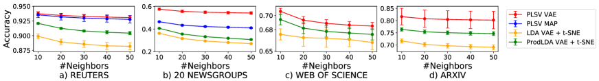
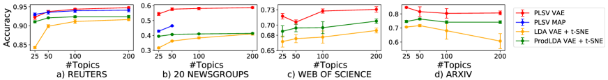
Figure 2: $k$-NN accuracy in the visualization space with different number of nearest neighbors $k$ ($Z=50$ topics). For some settings, PLSV-MAP does not return any results even after 24 hours of running.

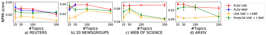
Figure 3: $k$-NN accuracy in the visualization space with different number of topics $Z$ ($k=10$). For some settings, PLSV-MAP does not return any results even after 24 hours of running.

Figure 4: Topic coherence based on NPMI with different number of topics $Z$. For some settings, PLSV-MAP does not return any results even after 24 hours of running.

4.2 Topic Coherence

We quantitatively measure the quality of topic models produced by all methods in terms of topic coherence. The objective is to show that while having better visualization quality, PLSV-VAE also gains comparable, if not better, topic coherence. For topic coherence evaluation, we use Normalized Pointwise Mutual Information (NPMI) which has been shown to be correlated with human judgments [Lau et al., 2014]. NPMI is computed as follows:

$$NPMI(w_{i},w_{j})=\frac{\log\frac{p(w_{i},w_{j})}{p(w_{i})p(w_{j})}}{-\log p(w_{i},w_{j})}$$ (10)

We estimate $p(w_{i},w_{j})$, $p(w_{i})$, and $p(w_{j})$ using Wikipedia 7-gram dataset created from the Wikipedia dump data as of June 2008 version. NPMI of a topic is computed as an average of the pairwise NPMI of its top 10 words. For each method, we average NPMI of its topics. Figure 4 shows topic coherence NPMI of all methods. As we can see, PLSV-VAE finds topics as good as those found by other methods, and in some settings, PLSV-VAE can find significantly better topics. For a qualitative evaluation of topic quality, we show some example topics found by PLSV-VAE in Figure 11.

4.3 Visualization Examples

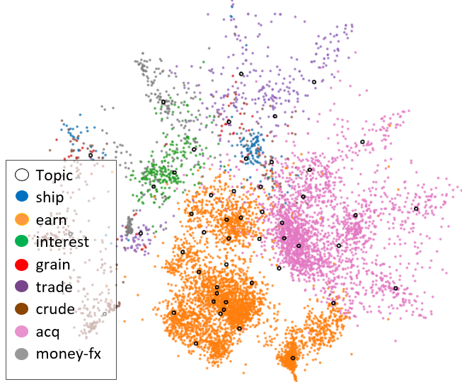
(a) Reuters (PLSV-MAP)

(b) Reuters (PLSV-VAE)

Figure 5: Visualization of Reuters by a) PLSV-MAP b) PLSV-VAE.

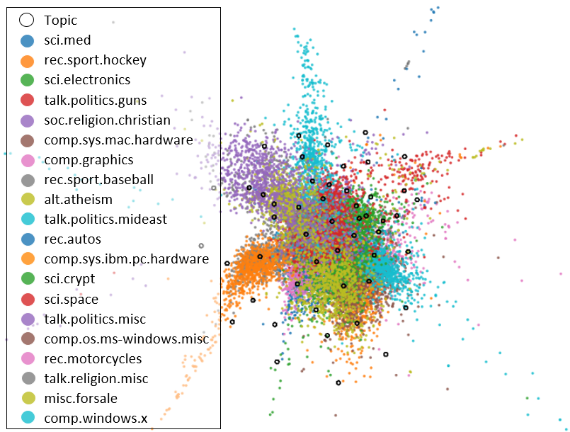
(c) 20 Newsgroups (PLSV-MAP)

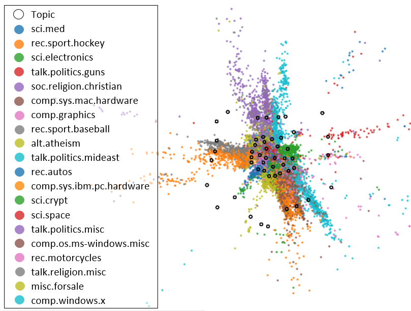
(d) 20 Newsgroups (PLSV-VAE)

Figure 6: Visualization of 20 Newsgroups by a) PLSV-MAP b) PLSV-VAE.

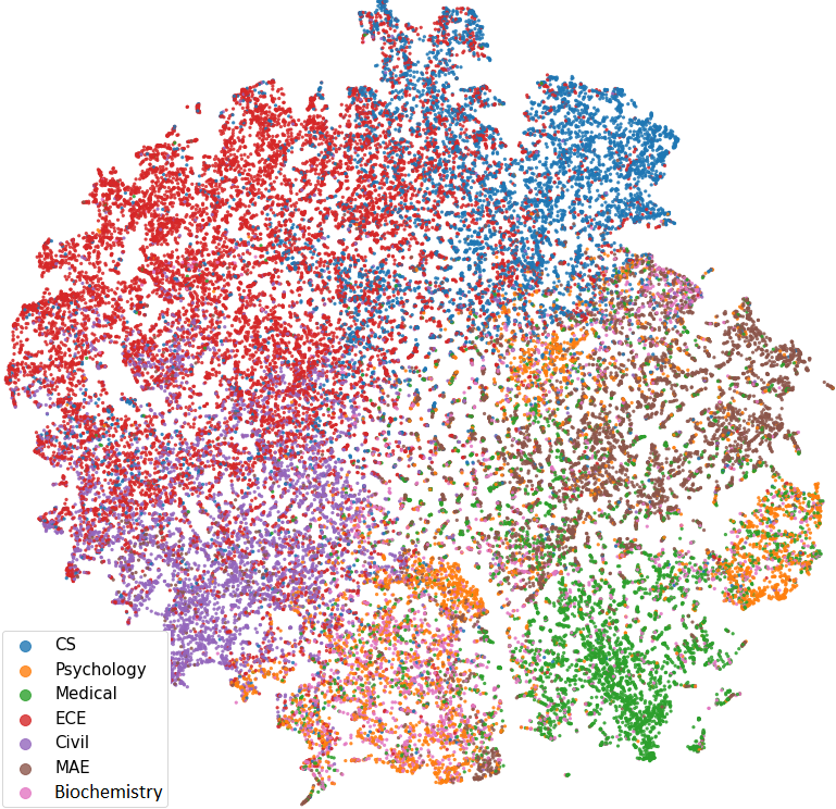
(a) Web of Science (ProdLDA-VAE + t-SNE)

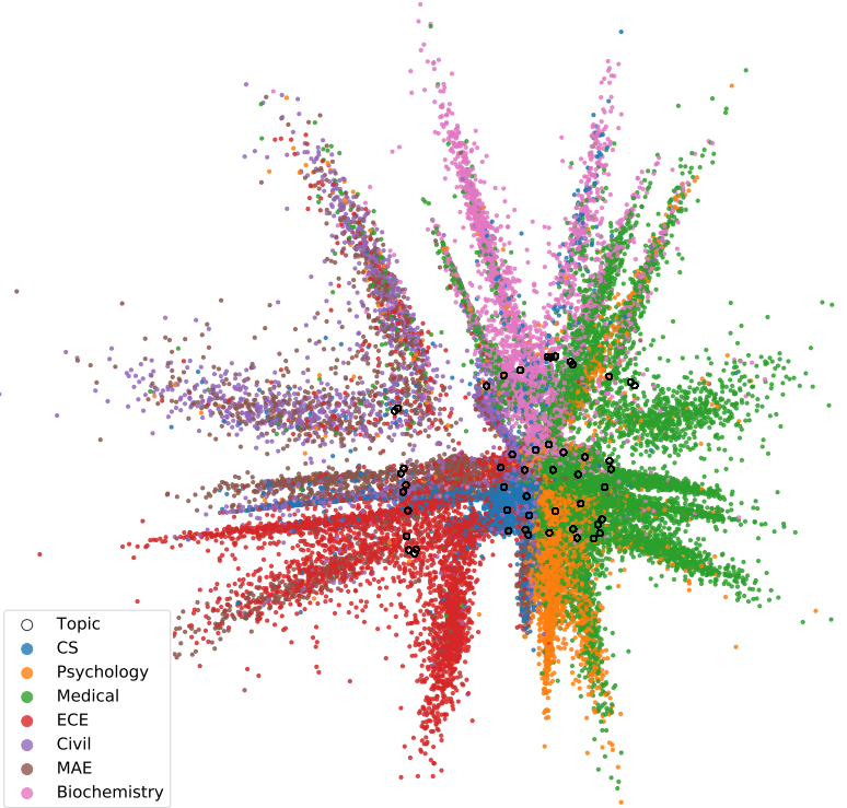
(b) Web of Science (PLSV-VAE)

Figure 7: Visualization of Web of Science by a) ProdLDA-VAE + t-SNE b) PLSV-VAE.

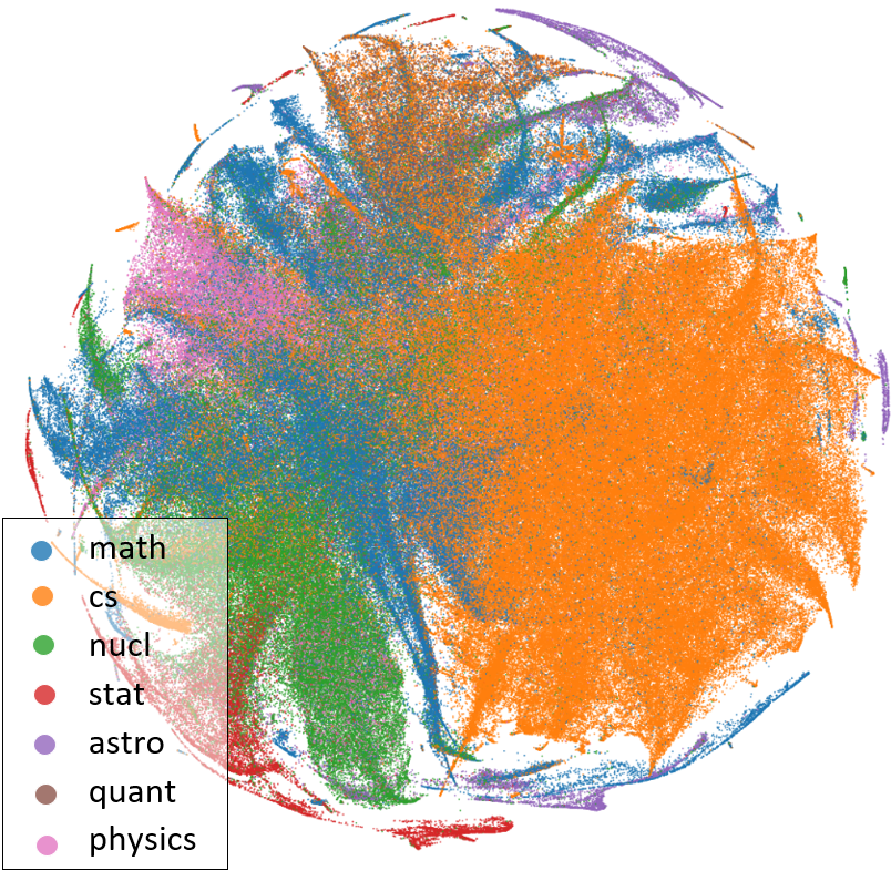
(a) Arxiv (ProdLDA-VAE + t-SNE)

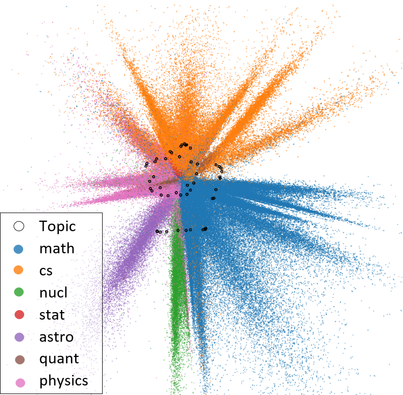
(b) Arxiv (PLSV-VAE)

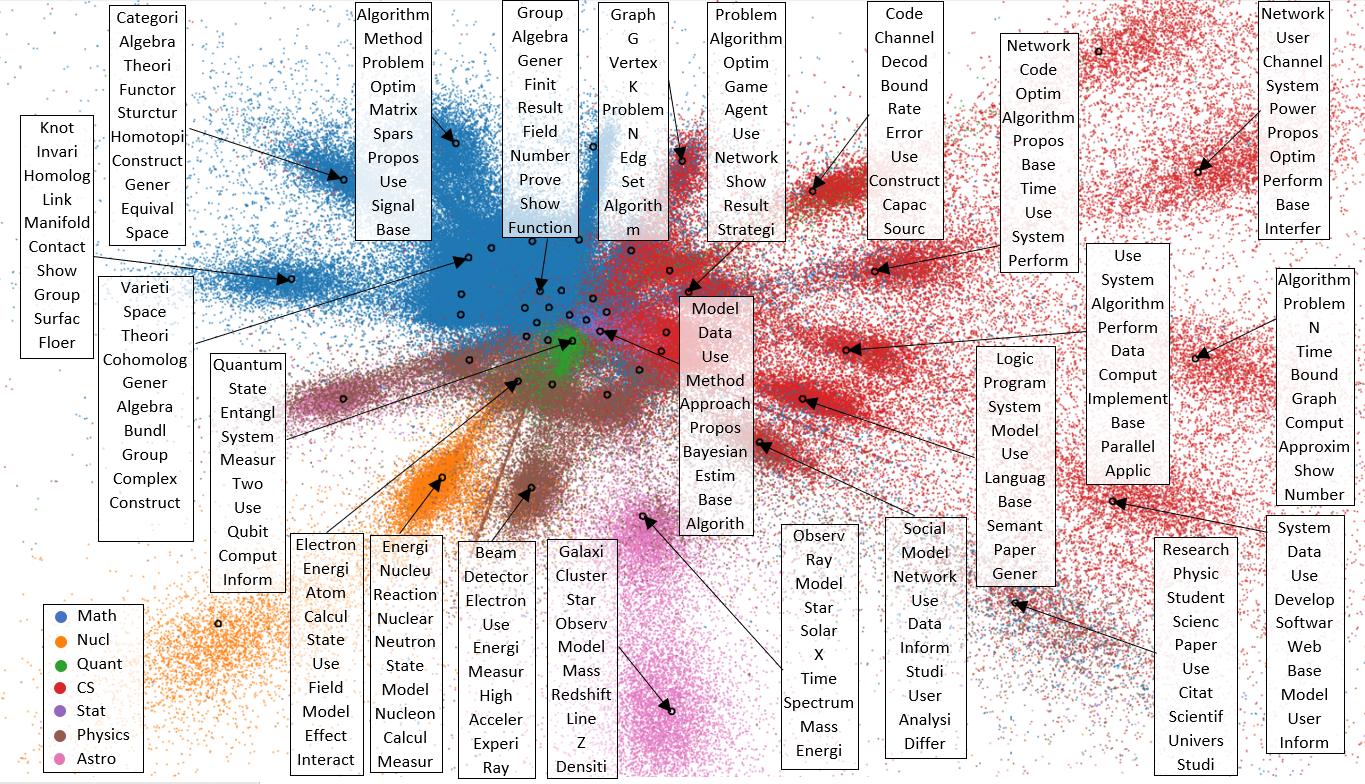
Figure 8: Visualization of Arxiv by a) ProdLDA-VAE + t-SNE b) PLSV-VAE.

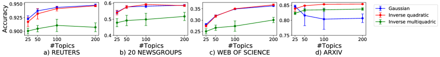
Figure 9: Visualization and topics found by PLSV-VAE (Inverse quadratic) on Arxiv ($Z=50$ topics).

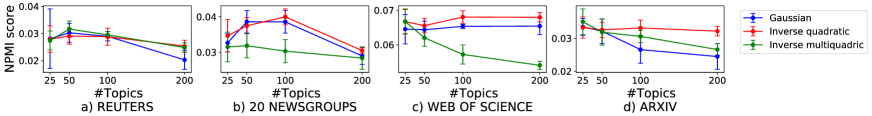
Figure 10: $k$-NN accuracy in the visualization space by PLSV-VAE with different RBFs ($k=10$).

Figure 11: Topic coherence NPMI by PLSV-VAE with different RBFs (vary number of topics $Z$).

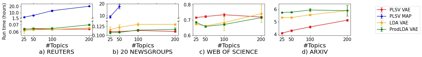
Figure 12: Running time comparison.

We compare visualizations produced by all methods qualitatively by showing some visualization examples. In these visualizations, each document is represented by a point and the color of each point indicates the class of that document. Figures 7 and 7 present visualizations by PLSV-MAP, PLSV-VAE on Reuters and 20 Newsgroups. We see that PLSV-VAE can find meaningful clusters of documents. For example, PLSV-VAE in Figure 7(b) separates well the eight classes into different clusters such as the pink cluster for acq, the orange cluster for earn, and the brown cluster for crude. The visualization by PLSV-MAP in Figure 7(a) also shows clear clusters but it runs much slower than PLSV-VAE as shown in Section 4.5. Figure 7 presents visualization outputs for 20 Newsgroups. For this more challenging dataset, PLSV-VAE produces better-separated clusters, as compared to PLSV-MAP. For example, baseball and hockey are mixed in Figure 7(a) by PLSV-MAP but these classes are separated better in Figure 7(b) by PLSV-VAE. We do not show visualizations of Web of Science and Arxiv by PLSV-MAP because it fails to return any results even after 24 hours of running. We instead show visualizations of these two large datasets by PLSV-VAE and ProdLDA-VAE + t-SNE in Figures 7 and 11. As we can see, visualizations by PLSV-VAE are more intuitive than the ones by ProdLDA-VAE + t-SNE, which supports the outperformance of the joint approach over the pipeline approach.

4.4 Comparing Different Radial Basis Functions

Since our method is black box, we can quickly explore PLSV-VAE model with different assumptions. In this section, we show how different RBFs affect the performance of PLSV-VAE. Besides PLSV-VAE with Gaussian RBF, we implement another two variants of PLSV-VAE that uses two other RBFs: Inverse quadratic and Inverse multiquadric RBFs. We choose these two because, similar to Gaussian, they support the assumption that the $z$th topic proportion of document $n$ is high when document coordinate $x_{n}$ is close to topic coordinate $\phi_{z}$. For these model changes, we do not need to perform a mathematical rederivation, but we only need to change a few lines of code of PLSV-VAE (Gaussian). Figures 11 and 11 show the $k$-NN accuracy and topic coherence of PLSV-VAE with different RBFs. In general, PLSV-VAE with Gaussian or Inverse quadratic RBFs consistently produces good performance across datasets. In some cases, Inverse quadratic produces better results.

4.5 Topic Examples and Running Time Comparison

To qualitatively evaluate the topics, in Figure 11, we show visualization and topic examples generated by PLSV-VAE (Inverse quadratic) on Arxiv. In the visualization, each black empty circle represents a topic that is associated with a list of top 10 words. We see that the topics are meaningful and reflect different research subdomains discussed in the Arxiv papers. For example, many topics are studied in the CS domain such as “graph, g, vertex, k”, “model, data, use, method”, and “logic, program, system”. For the Astro domain, we have topics like “galaxi, cluster, star”, and ”observ, ray, model, star”. Topics such as “energi, nucleu, reaction” and “electron, energi, atom” are discussed in the Nucl domain. By allowing the semantics to be infused in the visualization space, users can now not only see the documents but also their topics. The joint nature of the model may lead to potential applications in different visual text mining tasks.

Finally, we show the running time of all the methods in Figure 12. As expected, PLSV-MAP running on a single core is very slow and it fails to return any results on large datasets even after 24 hours of running. PLSV-VAE runs much faster. It only needs about 5 hours for 200 topics on the largest dataset Arxiv. For completeness, we also include the running time of LDA-VAE, and ProdLDA-VAE. PLSV-VAE is as fast as these methods. In summary, PLSV-VAE can find good topics and visualization while it can scale well to large datasets, which will increase its usability in practice.

5 Conclusion

We propose, to the best of our knowledge, the first fast AEVB based inference method for jointly learning topics and visualization. In our approach, we design a decoder that includes a normalized RBF network connected to a linear neural network. These networks are parameterized by topic coordinates and word probabilities, ensuring that they are shared across all documents. Due to our method’s black box nature, we can quickly experiment with different RBFs with minimal reimplementation effort. Our extensive experiments on four real-world large datasets show that PLSV-VAE runs much faster than PLSV-MAP while gaining better visualization quality and comparable topic coherence.

References

- [Bishop, 1995] Christopher M Bishop. 1995. Neural networks for pattern recognition. Oxford University Press.
- [Blei et al., 2003] David M Blei, Andrew Y Ng, and Michael I Jordan. 2003. Latent dirichlet allocation. Journal of machine Learning research, 3(Jan):993–1022.
- [Blei et al., 2007] David M Blei, John D Lafferty, et al. 2007. A correlated topic model of science. The Annals of Applied Statistics, 1(1):17–35.
- [Cardoso-Cachopo, 2007] Ana Cardoso-Cachopo. 2007. Improving Methods for Single-label Text Categorization. PdD Thesis, Instituto Superior Tecnico, Universidade Tecnica de Lisboa.
- [Casale et al., 2018] Francesco Paolo Casale, Adrian Dalca, Luca Saglietti, Jennifer Listgarten, and Nicolo Fusi. 2018. Gaussian process prior variational autoencoders. In Advances in Neural Information Processing Systems, pages 10369–10380.
- [Choo et al., 2013] Jaegul Choo, Changhyun Lee, Chandan K Reddy, and Haesun Park. 2013. Utopian: User-driven topic modeling based on interactive nonnegative matrix factorization. IEEE transactions on visualization and computer graphics, 19(12):1992–2001.
- [He et al., 2019] Junxian He, Daniel Spokoyny, Graham Neubig, and Taylor Berg-Kirkpatrick. 2019. Lagging inference networks and posterior collapse in variational autoencoders. In International Conference on Learning Representations (ICLR), New Orleans, LA, USA, May.
- [Hofmann, 1999] Thomas Hofmann. 1999. Probabilistic latent semantic analysis. In UAI.
- [Ioffe and Szegedy, 2015] Sergey Ioffe and Christian Szegedy. 2015. Batch normalization: Accelerating deep network training by reducing internal covariate shift. In Francis Bach and David Blei, editors, Proceedings of the 32nd International Conference on Machine Learning, volume 37 of Proceedings of Machine Learning Research, pages 448–456, Lille, France, 07–09 Jul. PMLR.
- [Iwata et al., 2008] Tomoharu Iwata, Takeshi Yamada, and Naonori Ueda. 2008. Probabilistic latent semantic visualization: topic model for visualizing documents. In Proceedings of the 14th ACM SIGKDD international conference on Knowledge discovery and data mining, pages 363–371.
- [Kalai et al., 2010] Adam Tauman Kalai, Ankur Moitra, and Gregory Valiant. 2010. Efficiently learning mixtures of two gaussians. In Proceedings of the forty-second ACM symposium on Theory of computing, pages 553–562.
- [Kim et al., 2019] Hannah Kim, Dongjin Choi, Barry Drake, Alex Endert, and Haesun Park. 2019. Topicsifter: Interactive search space reduction through targeted topic modeling. In 2019 IEEE Conference on Visual Analytics Science and Technology (VAST), pages 35–45. IEEE.
- [Kingma and Welling, 2014a] Diederik P. Kingma and Max Welling. 2014a. Auto-encoding variational bayes. In 2nd International Conference on Learning Representations, ICLR 2014, Banff, AB, Canada, April 14-16, 2014, Conference Track Proceedings.
- [Kingma and Welling, 2014b] Diederik P. Kingma and Max Welling. 2014b. Auto-encoding variational bayes. CoRR, abs/1312.6114.
- [Kowsari et al., 2017] Kamran Kowsari, Donald E Brown, Mojtaba Heidarysafa, Kiana Jafari Meimandi, , Matthew S Gerber, and Laura E Barnes. 2017. Hdltex: Hierarchical deep learning for text classification. In Machine Learning and Applications (ICMLA), 2017 16th IEEE International Conference on. IEEE.
- [Lau et al., 2014] Jey Han Lau, David Newman, and Timothy Baldwin. 2014. Machine reading tea leaves: Automatically evaluating topic coherence and topic model quality. In Proceedings of the 14th Conference of the European Chapter of the Association for Computational Linguistics, pages 530–539.
- [Le and Akoglu, 2019] Tuan Le and Leman Akoglu. 2019. Contravis: contrastive and visual topic modeling for comparing document collections. In The World Wide Web Conference, pages 928–938.
- [Le and Lauw, 2014a] Tuan MV Le and Hady W Lauw. 2014a. Manifold learning for jointly modeling topic and visualization. In Twenty-Eighth AAAI Conference on Artificial Intelligence.
- [Le and Lauw, 2014b] Tuan MV Le and Hady W Lauw. 2014b. Semantic visualization for spherical representation. In Proceedings of the 20th ACM SIGKDD international conference on Knowledge discovery and data mining, pages 1007–1016.
- [Le and Lauw, 2016] Tuan MV Le and Hady W Lauw. 2016. Semantic visualization with neighborhood graph regularization. Journal of Artificial Intelligence Research, 55:1091–1133.
- [Lin et al., 2019] Shuyu Lin, Ronald Clark, Robert Birke, Niki Trigoni, and Stephen J. Roberts. 2019. Wise-ale: Wide sample estimator for aggregate latent embedding. In Deep Generative Models for Highly Structured Data, ICLR 2019 Workshop, New Orleans, Louisiana, United States, May 6, 2019. OpenReview.net.
- [Maaten and Hinton, 2008] Laurens van der Maaten and Geoffrey Hinton. 2008. Visualizing data using t-sne. Journal of machine learning research, 9(Nov):2579–2605.
- [Ramage et al., 2009] Daniel Ramage, Evan Rosen, Jason Chuang, Christopher D Manning, and Daniel A McFarland. 2009. Topic modeling for the social sciences. In NIPS 2009 workshop on applications for topic models: text and beyond, volume 5, page 27.
- [Ranganath et al., 2014] Rajesh Ranganath, Sean Gerrish, and David M. Blei. 2014. Black box variational inference. ArXiv, abs/1401.0118.
- [Razavi et al., 2019] Ali Razavi, Aäron van den Oord, Ben Poole, and Oriol Vinyals. 2019. Preventing posterior collapse with delta-vaes. In 7th International Conference on Learning Representations, ICLR 2019, New Orleans, LA, USA, May 6-9, 2019. OpenReview.net.
- [Srivastava and Sutton, 2017] Akash Srivastava and Charles A. Sutton. 2017. Autoencoding variational inference for topic models. In ICLR.
- [Tang et al., 2016] Jian Tang, Jingzhou Liu, Ming Zhang, and Qiaozhu Mei. 2016. Visualizing large-scale and high-dimensional data. In Proceedings of the 25th international conference on world wide web, pages 287–297.
- [Tkachenko and Lauw, 2019] Maksim Tkachenko and Hady W Lauw. 2019. Comparelda: A topic model for document comparison. In Proceedings of the AAAI Conference on Artificial Intelligence, volume 33, pages 7112–7119.