Rotations of the polarization of a gravitational wave propagating in Universe

Abstract

In this paper, we study the polarization of a gravitational wave (GW) emitted by an astrophysical source at a cosmic distance propagating through the Friedmann-Lemaître-Robertson-Walk (FLRW) universe. By considering the null geodesic deviations, we first provide a definition of the polarization of the GW in terms of the Weyl scalars with respect to a parallel-transported frame along the null geodesics, and then show explicitly that, due to different effects of the expansion of the universe on the two polarization modes, the so-called “+” and “$\times$” modes, the polarization angle of the GW changes generically, when it is propagating through the curved background. More precisely, due to the presence of the matter field of the FLRW background, both of the “$\times$” and “+” modes can get amplified or diluted, depending on their waveforms, so in principle the effects to the “$\times$” modes are different from those to the “+” modes. As a result, the polarization angle will change along the wave path, regardless of which source it is. As a concrete example, we directly compute the polarization angle in a binary system, and show that different epochs, radiation-, matter- and $\Lambda$-dominated, have different effects on the polarization. In particular, for a GW emitted by a binary system, we find explicitly the relation between the change of the polarization angle $|\Delta\varphi|$ and the redshift $z_{s}$ of the source in different epochs. In the $\Lambda$CDM model, we find that the order of $|\Delta\varphi|{\eta_{0}F}$ is typically $O(10^{-3})$ to $O(10^{3})$, depending on the values of $z_{s}$, where $\eta_{0}$ is the (comoving) time of the current universe, and $F\equiv\Big{(}\frac{5}{256}\frac{1}{\tau_{obs}}\Big{)}^{3/8}\left(G_{N}M_{c}\right)^{-5/8}$ with $\tau_{obs}$ and $M_{c}$ being, respectively, the time to coalescence in the observer’s frame and the chirp mass of the binary system. The typical value of $|\Delta\varphi|$ for LIGO-Virgo sources is $10^{-21}$. Hence, it may not be easily detected with current detectors.

I Introduction

With the detection of gravitational waves (GWs) by the LIGO collaboration GW150914 ; GW151226 , a new era, the gravitational wave astronomy, began, after exactly 100 years since Einstein first predicted the existence of GWs Einstein1916 by using his brand new theory of general relativity, established only one year earlier. The masses of the two binary black holes (BBHs) in the event GW151226 were, respectively, $14M_{\odot}$ and $7M_{\odot}$ GW151226 , well in the range of stellar-mass black holes known so far BHs . On the other hand, in the event GW150914 GW150914 , the masses of the two black holes were, respectively, $36M_{\odot}$ and $29M_{\odot}$, which are much more massive than the known ones BHs . This has already stimulated lots of interest and various scenarios have been proposed, including their formation from very massive stars ($50-100M_{\odot}$) MassiveStars , PopIII stars PopIIIStars , and primordial black holes PBHs (see alsoT.Z. Wang ). Despite of the difference among the masses of BBHs in these two events, the distances of them to Earth are almost the same, about $400$Mpc, which corresponds to a redshift of $z\simeq 0.09$ GW150914 ; GW151226 . After that, LIGO/Virgo scientific collaborations detected dozen more GWs GW190814 ; 2019 ; GWs19a ; GWs19b ; Abbott:2017vtc ; Abbott:2017gyy ; Abbott:2017oio ; TheLIGOScientific:2017qsa , including possibly the coalescence of neutron-star (NS)/BH binary, although some details of these detections have not been released yet LIGO . Over the next few years, the advanced LIGO and Virgo will continuously increase their sensitivities, and once at their designed goals, together with other detectors of the second generation, such as KAGRA KAGRA , they could be able to detect heavy BBHs up to redshifts of unity. The third generation detectors, both ground and space based, such as the Einstein Telescope ET , Cosmic Explorer CE , LISA LISA , Taiji Taiji , Tianqin Tianqin , and DECIGO DEIGO , will substantially increase their sensitivities and allow us to detect GWs from sources up to redshifts of $z\simeq 20$, well within the epoch of reionization VE . Therefore, the studies of such GWs and their sources, among other things, will open a new window to explore the early universe.

Such studies are normally divided into two different zones, the generation and propagation zones YYP . The propagation zone is further divided into three different phases, the inspiral, plunge/merger and ringdown phases. In the inspiral phase, the post-Newtonian (PN) approximations are usually used, while in merger phase, the gravitational field is very strong and the field equations (of Einstein as well as of other theories), become highly nonlinear, and heavy numerical calculations are often inevitably used. In the ringdown phase, quasi-normal modes (QNM) analysis is found sufficient.

When GWs are far from their sources (in the far propagation zone), they become very weak, and can be considered as linear perturbations. Previous studies were mainly focused on perturbations in the Minkowski background GWs , but recently studies of perturbations in the Friedmann-Lemaître-Robertson-Walk (FLRW) background have started to attract attention ABK15 ; Chu15 ; BGY15 ; KR16 ; TW16 (See also DBBE ).

In particular, for a GW generated by an astrophysical source with a distribution of matter in a finite region, such as an inspiraling compact binary system, it can be considered as perturbations on the FLRW background $\hat{g}_{\mu\nu}\equiv a^{2}\eta_{\mu\nu}$,

$$g_{\mu\nu}=a^{2}(\eta)\left(\eta_{\mu\nu}+\epsilon h_{\mu\nu}\right),$$ (1.1)

where $\eta_{\mu\nu}={\mbox{diag.}}\left(1,-1,-1,-1\right)$, $\eta$ denotes the conformal time of the FLRW universe, and $\left|\epsilon h_{\mu\nu}\right|\ll 1$. In this paper, we shall use the notations and conventions of dInverno , and in particular, we shall set the speed of light to unity, $c=1$. In the transverse-traceless (TT) gauge,

$$h_{\mu\nu}dx^{\mu}dx^{\nu}=D_{ij}dx^{i}dx^{j},$$ (1.2)

with $\delta^{ij}D_{ij}=0=\partial^{i}D_{ij}$, the linear perturbations $D_{ij}$’s equations are given by Chu15 ,

$${\Box}D_{ij}=16\pi G_{N}\Pi_{ij},$$ (1.3)

where ${\Box}\equiv\hat{g}^{\mu\nu}\hat{\nabla}_{\mu}\hat{\nabla}_{\nu}$, $\hat{\nabla}_{\mu}$ denotes the covariant derivative with respect to $\hat{g}_{\mu\nu}$, and $\Pi_{ij}$ denotes the part of matter perturbations $\delta T^{i}_{j}$, subjected to the TT constraints, $\delta^{ij}\Pi_{ij}=0=\partial^{i}\Pi_{ij}$. When far from the source, $\left|\vec{x}\right|\gg D$, where $D$ denotes the spatial extent of the source, and $\left|\vec{x}\right|\;\left[\equiv\sqrt{x^{2}+y^{2}+z^{2}}\right]$ is the comoving distance between the center of the source and the observer.

In the FLRW background (1.1), when GWs propagate through this curved space-time, an additional term appeared due to the scattering off the curved backgorund, the “backscattering waves” or “tails” $D_{ij}$ consists of two parts: one travels along the light-cone, denoted by $D_{ij}^{(\gamma)}$, which will be referred to as the propagation (or direct) part, and the other travels inside the light-cone, denoted by $D^{(tail)}_{ij}$, the so-called tails as shown in Fig. 1. They are given, respectively, by,

$$D_{ij}^{(\gamma)}=\frac{4G_{N}F_{ij}^{(\gamma)}(v)}{\left|\vec{x}\right|a(\eta)},\;\;\;D_{ij}^{(tail)}=\frac{4G_{N}F_{ij}^{(tail)}(\eta,\vec{x})}{a(\eta)},$$ (1.4)

where $v\equiv\frac{1}{\sqrt{2}}(\eta-\left|\vec{x}\right|)$, and

$$F_{ij}^{(\gamma)}(v) \equiv \int_{\mathbb{R}^{3}}{\mathrm{d}^{3}\vec{x}^{\prime}a^{3}(v)\Pi_{ij}\left(v,\vec{x}^{\prime}\right)},$$

$$F_{ij}^{(tail)}(\eta,\vec{x}) \equiv \int{a^{3}(\eta^{\prime})\mathrm{d}\eta^{\prime}}\int_{\mathbb{R}^{3}}{\mathrm{d}^{3}\vec{x}^{\prime}\Theta(\hat{\sigma})\Pi_{ij}\left(\eta^{\prime},\vec{x}^{\prime}\right)}\times\frac{\partial J(\eta,\eta^{\prime};\hat{\sigma})}{\partial\hat{\sigma}},$$ (1.5)

where $\mathbb{R}^{3}$ is the region of source, and $\Theta(x)$ denotes the Heaviside function,

$$\Theta(x)=\begin{cases}1,&x\geq 0,\cr 0,&x<0.\cr\end{cases}$$ (1.6)

And $\hat{\sigma}\equiv\left[(\eta-\eta^{\prime})^{2}-(z-z^{\prime})^{2}-(\vec{x}_{\bot}-\vec{x}_{\bot}^{\prime})^{2}\right]/2,\;\vec{x}\equiv(z,\vec{x}_{\bot}),\;\vec{x}_{\bot}\equiv(x,y)$. The function $J(\eta,\eta^{\prime};\hat{\sigma})$ satisfies the equation,

$${\cal{W}}_{2}{(\eta,{z})}J(\eta,\eta^{\prime};\hat{\sigma})={\cal{W}}_{2}{(\eta^{\prime},{z}^{\prime})}J(\eta,\eta^{\prime};\hat{\sigma})=0,$$ (1.7)

with

$${\cal{W}}_{2}{(\eta,z)}\equiv\partial^{2}_{\eta}-\partial^{2}_{z}-\frac{a^{\prime\prime}(\eta)}{a(\eta)},$$ (1.8)

where $a^{\prime\prime}(\eta)\equiv d^{2}a(\eta)/d\eta^{2}$, etc. When $a(\eta)$ is a constant, for which the background becomes the Minkowski spacetime, the last term of Eq.(1.8) vanishes, so Eq.(1.7) reduces to $(\partial^{2}_{\eta}-\partial^{2}_{z})J(\eta,\eta^{\prime};\hat{\sigma})=0$, which represents waves propagating along the light-cone $\eta=\pm z$, that is, the tail part reduces to the direct part, and the corresponding GWs all move exactly along the light-cones.

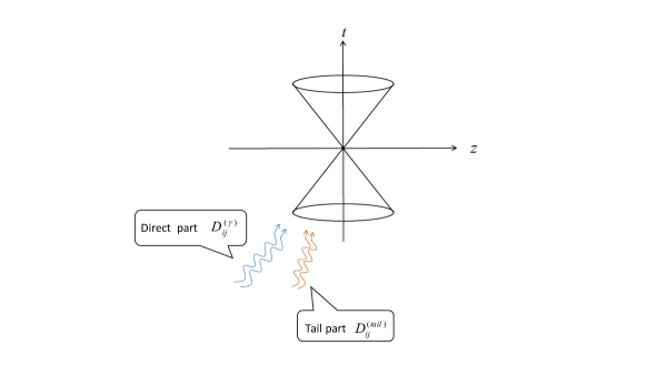
Figure 1: $D_{ij}$ consists of two parts: one is the propagation (or direct) part $D_{ij}^{(\gamma)}$ which travels along the light-cone, and the other is the tail part $D^{(tail)}_{ij}$ which travels inside the light-cone.

In this paper, we shall study the polarizations of GWs produced by an astrophysical source, which propagate through our universe over a cosmic distance. As a first step, we shall assume that our universe is homogeneous and isotropic. The efforts of the inhomogeneity will be considered somewhere else JF20 .

The rest of this paper is organized as follows. In Section II, assuming that the GWs are far from their sources, we show how to define the polarization angle of the GW propagating through the flat FLRW background at a cosmic distance. In Section III, different epochs, in which the universe is dominated by different components of matter field, are considered. In particular, we calculate explicitly the changes of the polarization angle in each of these epochs. Our main conclusions are summarized in section IV.

There are also four appendices, A, B, C and D, in which some mathematical calculations involved in this paper are given in detail. In particular, in Appendix C we consider the timelike geodesics deviations, from which we define the polarization of a GW propagating through the flat FLRW universe, and show that it is the same as that obtained by considering null geodesic deviations studied in Section II.

II Polarizations of Gravitational Waves

In the rest of this paper, we shall assume that the GWs are far from their sources, so they are well-described by Eqs.(1.4)-(1.8). In addition, we shall choose the coordinates so that the $z$-axis is passing through the observer and the center of the source. Then, the transverse-traceless conditions lead to,

$$D_{22} = -D_{33}\equiv h_{+},\quad D_{23}=D_{32}\equiv-h_{\times},$$

$$D_{i1} = 0,\;(i=1,2,3),$$ (2.1)

with

$$h_{\sigma}(\eta,\vec{x})\equiv\frac{{\cal{P}}_{\sigma}(v)}{{\cal{R}}}+\frac{{\cal{T}}_{\sigma}(u,v)}{a^{n}}+{\cal{O}}\left(\frac{1}{|\vec{x}|^{2}}\right),$$ (2.2)

where $\sigma=+,\times,\;u\equiv{\frac{1}{\sqrt{2}}}(\eta+\left|\vec{x}\right|)$, and ${\cal{R}}\equiv a(\eta)|\vec{x}|$ is the physical distance from the center of the source to the observer, $n$ is a constant, and

$${\cal{T}}_{\sigma}(u,v)\propto\int_{\mathbb{R}^{3}}{\mathrm{d}^{3}\vec{x}^{\prime}\Theta(\hat{\sigma})\Pi_{ij}\left(\eta^{\prime},\vec{x}^{\prime}\right)}\frac{\partial J(\eta,\eta^{\prime};\hat{\sigma})}{\partial\hat{\sigma}}.~{}~{}~{}$$ (2.3)

In the radiation-dominated epoch we have ${\cal{T}}_{\sigma}(u,v)=0$, while in the de Sitter spacetime, or the matter-dominated epoch, we have ${\cal{T}}_{\sigma}(u,v)\not=0$, but with $n=0,3/2$, respectively Chu15 .

In writing the above expressions, we expanded the direct part $D_{ij}^{(\gamma)}(t,\vec{x})$ only to the first-order of $1/|\vec{x}|$. ${\cal{P}}_{\sigma}(v)$ is related to the integration of the direct part of the source via the relation,

$${\cal{P}}_{\sigma}(v)\simeq G_{N}\int_{\mathbb{R}^{3}}{\mathrm{d}^{3}\vec{x}^{\prime}a^{3}(v)\Pi_{ij}\left(v,\vec{x}^{\prime}\right)},$$ (2.4)

which propagates along the light-cone, $v=$ Constant, toward the observer in the increasing direction of $z$. On the other hand, ${\cal{T}}_{\sigma}(u,v)$ denotes the tails propagating inside the light-cone, due to the backscattering of the GWs over the FLRW background. Note that we keep this part to the linear order of ${\cal{T}}_{\sigma}$ without expanding it further in terms of $1/|\vec{x}|$.

Considering Eqs.(1.1), (1.2) and (II), we find that the metric of such space-times takes the form,

$$\mathrm{d}s^{2} = e^{-M}\left(\mathrm{d}\eta^{2}-\mathrm{d}z^{2}\right)-e^{-U}\left\{e^{V}\cosh{W}\mathrm{d}x^{2}-2\sinh{W}\mathrm{d}x\mathrm{d}y+e^{-V}\cosh{W}\mathrm{d}y^{2}\right\},$$ (2.5)

where

$$M = U=-2\ln a,\quad V=\epsilon h_{+},\quad W=\epsilon h_{\times}.$$ (2.6)

Then, the analysis of propagation and polarizations of GWs in the Universe can follow the one given in Szekeres72 ; Griffiths76a ; Griffiths:1991zp ; WThesis ; Wang91 ; HFZ19 , which is crucially based on the following decompositions of the Riemann tensor,

$$R_{\mu\nu\lambda\beta} = C_{\mu\nu\lambda\beta}+\frac{R}{6}\left(g_{\mu\beta}g_{\nu\lambda}-g_{\mu\lambda}g_{\nu\beta}\right)+\frac{1}{2}\Big{(}g_{\mu\lambda}R_{\nu\beta}+g_{\nu\beta}R_{\mu\lambda}-g_{\nu\lambda}R_{\mu\beta}-g_{\mu\beta}R_{\nu\lambda}\Big{)},$$ (2.7)

where $R_{\mu\nu}$ and $R$ denote, respectively, the Ricci tensor and scalar, and $C_{\mu\nu\lambda\beta}$ is the Weyl tensor. The latter is considered as representing pure gravitational fields, while $R_{\mu\nu}$ is connected to the energy-momentum tensor $T_{\mu\nu}$ through the Einstein field equations $R_{\mu\nu}=8\pi G_{N}\left(T_{\mu\nu}-g_{\mu\nu}T/2\right)$, which is usually considered as the spacetime curvature produced by matter.

In terms of $C_{\mu\nu\lambda\beta}$ and $R_{\mu\nu}$, the Bianchi identities take the form,

$$\nabla^{\alpha}C_{\mu\nu\lambda\alpha}=J_{\mu\nu\lambda},$$ (2.8)

which represents the interaction between matter and pure gravitational fields (represented by the Weyl tensor $C_{\mu\nu\lambda\beta}$), where

$$J_{\mu\nu\lambda}\equiv\nabla_{[\nu}R_{\mu]\lambda}-\frac{1}{6}g_{\lambda[\mu}\nabla_{\nu]}R,$$ (2.9)

is directly related to the energy-momentum tensor $T_{\mu\nu}$ through the Einstein field equations, with $[A,B]\equiv(AB-BA)/2$. Clearly, in vacuum we have $J_{\mu\nu\lambda}=0$.

To study the phenomena, it is found very convenient to use the Newman-Penrose formula NP62 , a tetrad formula but with a particular choice of the tetrad,

$$l^{\mu} \equiv B\left(\delta^{\mu}_{\eta}-\delta^{\mu}_{z}\right),\quad n^{\mu}\equiv A\left(\delta^{\mu}_{\eta}+\delta^{\mu}_{z}\right),$$

$$m^{\mu} \equiv \zeta^{2}\delta^{\mu}_{2}+\zeta^{3}\delta^{\mu}_{3},\quad\bar{m}^{\mu}\equiv\overline{m^{\mu}},$$ (2.10)

where an overline/bar denotes the complex conjugate, and

$$\zeta^{2} \equiv \frac{1{-}{\cal{G}}}{\sqrt{2}a},\;\;\zeta^{3}\equiv\frac{i(1{+}{\cal{G}})}{\sqrt{2}a},$$

$$AB \equiv \frac{1}{2a^{2}},\quad{\cal{G}}\equiv\frac{\epsilon}{2}\left(h_{+}-ih_{\times}\right).$$ (2.11)

It can be shown that, to the leading order of $\epsilon$, each of $l^{\mu}$ and $n^{\mu}$ defines a null geodesic congruence,

$$l^{\nu}\nabla_{\nu}l^{\mu} = -\frac{BA_{,\eta}}{A}l^{\mu}+{\cal{O}}\left(\epsilon^{2}\right),$$

$$n^{\nu}\nabla_{\nu}n^{\mu} = -\frac{AB_{,\eta}}{B}n^{\mu}+{\cal{O}}\left(\epsilon^{2}\right),$$ (2.12)

where $\nabla_{\nu}$ denotes the covariant derivative with respect to $g_{\mu\nu}$, and $A_{,\eta}\equiv\partial A/\partial\eta$, etc. Projecting the Weyl and Ricci tensors onto the above null tetrad, we find that the ten independent components of the Weyl tensor are given by the five Weyl (complex) scalars, $\Psi_{A}$, while the ten independent components of the Ricci tenor are given by the seven Ricci scalar, $\Phi_{AB}$, given explicitly in Appendix A for the metric Eq.(2.5). In particular, we have

$${\mbox{Re}}\left(\Psi_{0}\right) = {-}\frac{1}{8A^{2}a^{4}}\Bigg{\{}\frac{1}{{\cal{R}}}\Big{[}2{{\cal{P}}_{+,vv}}-2\sqrt{2}{{\cal{H}}}{{\cal{P}}_{+,v}}+({{\cal{H}}}^{2}-{{\cal{H}^{\prime}}}){{\cal{P}}_{+}}\Big{]}$$ (2.13)

$$~{}~{}~{}+\frac{1}{a^{n}}\Bigg{[}2{{\cal{T}}_{+,vv}}\left(1-\frac{x^{2}+y^{2}}{2z^{2}}\right)+\sqrt{2}n{{\cal{H}}}\Bigg{(}({{\cal{T}}_{+,u}}-{{\cal{T}}_{+,v}})\left(1-\frac{x^{2}+y^{2}}{2z^{2}}\right)$$

$$~{}~{}~{}-({{\cal{T}}_{+,u}}+{{\cal{T}}_{+,v}})\Bigg{)}+n(n{{\cal{H}}}^{2}-{{\cal{H}^{\prime}}}){{\cal{T}}_{+}}\Bigg{]}\Bigg{\}}\epsilon+{\cal{O}}\left(\epsilon^{2}\right),$$

$${\mbox{Im}}\left(\Psi_{0}\right) = \frac{1}{8A^{2}a^{4}}\Bigg{\{}\frac{1}{{\cal{R}}}\Bigg{[}2{{\cal{P}}_{\times,vv}}-2\sqrt{2}{{\cal{H}}}{{\cal{P}}_{\times,v}}+({{\cal{H}}}^{2}-{{\cal{H}^{\prime}}}){{\cal{P}}_{\times}}\Bigg{]}$$ (2.14)

$$~{}+\frac{1}{a^{n}}\Bigg{[}2{{\cal{T}}_{\times,vv}}\left(1-\frac{x^{2}+y^{2}}{2z^{2}}\right)+\sqrt{2}n{{\cal{H}}}\Bigg{(}({{\cal{T}}_{\times,u}}-{{\cal{T}}_{\times,v}})\left(1-\frac{x^{2}+y^{2}}{2z^{2}}\right)$$

$$~{}-({{\cal{T}}_{\times,u}}+{{\cal{T}}_{\times,v}})\Bigg{)}+n(n{{\cal{H}}}^{2}-{{\cal{H}^{\prime}}}){{\cal{T}}_{\times}}\Bigg{]}\Bigg{\}}\epsilon+{\cal{O}}\left(\epsilon^{2}\right),$$

where

$${\cal{P}}_{\sigma,v}=\frac{\mathrm{d}{\cal{P}}_{\sigma}(v)}{\mathrm{d}v},\;\;\;\;{\cal{H}}=\frac{a^{\prime}(\eta)}{a(\eta)},\;\;\;\;{\cal{H}}^{\prime}=\frac{\mathrm{d}{\cal{H}}}{\mathrm{d}\eta}.$$ (2.15)

The importance of the above decompositions is that each component of these scalars has its own physical interpretation. For example, $\Psi_{0}$ and $\Psi_{4}$ represent the gravitational waves propagating along the null geodesics, defined by $l^{\mu}$ and $n^{\mu}$, respectively, while $\Psi_{1}$ and $\Psi_{3}$ represent the longitudinal components, and $\Psi_{2}$ the Coulomb component Szekeres65 .

II.1 Polarizations of GWs

To study the polarization of GWs propagating in the FRLW background, let us consider null geodesic deviations. The main motivation of studying null geodesic deviations, instead of those timelike which are related to observations directly, is that GWs are traveling along their null geodesics before catching by the detectors. As shown in Wang91 ; WThesis , the considerations of null geodesic congruences will lead to the same definition for the polarization of a given GW. However, in Wang91 ; WThesis only plane gravitational wave (Petrov Type N)spacetimes were considered, and in what follows we will show that this is also true for the spacetimes considered here, by considering null geodesic deviations. In fact, in Appendix C we show that the definition of the polarization of a GW should be valid in any given spacetime, independent of its symmetry and the nature of the geodesic deviations, null or timelike.

To our purpose, in the following let us consider the null geodesic congruences formed by $l^{\mu}$. We construct the following four unity vectors,

$$e^{\mu}_{0} \equiv t^{\mu}\equiv\frac{1}{\sqrt{2}}(n^{\mu}+l^{\mu}),\quad e_{1}^{\mu}\equiv s^{\mu}\equiv\frac{1}{\sqrt{2}}(n^{\mu}-l^{\mu}),$$

$$e^{\mu}_{2} \equiv \frac{1}{\sqrt{2}}\left(m^{\mu}+\bar{m}^{\mu}\right),\quad e^{\mu}_{3}\equiv-\frac{i}{\sqrt{2}}\left(m^{\mu}-\bar{m}^{\mu}\right),$$

so that they form an orthogonal base

$$g_{\mu\nu}e^{\mu}_{a}e^{\nu}_{b}=\eta_{ab},$$ (2.17)

where $e^{\mu}_{a}\equiv\left(t^{\mu},s^{\mu},e^{\mu}_{2},e^{\mu}_{3}\right),(a=0,1,2,3)$, and $\eta_{ab}=\text{diag.}\left(1,-1,-1,-1\right)$.

Let $\eta^{\mu}$ be the geodesic deviation between two neighbor geodesics and $\eta^{\mu}l_{\mu}=0$. Then, after some tedious but straightforward calculations, we find that the null geodesic deviation is given by,

$$\frac{\mathrm{d}^{2}\eta^{\mu}}{\mathrm{d}\lambda^{2}} = -R^{\mu}_{\nu\lambda\beta}l^{\nu}\eta^{\lambda}l^{\beta}$$

$$= \Big{\{}\Big{[}\left(\Psi_{2}+\bar{\Psi}_{2}\right)-2\Phi_{11}+2\Lambda\Big{]}{(e^{\mu}_{0}-e^{\nu}_{1})(e^{\nu}_{0}-e^{\mu}_{1})}$$

$${-}\Phi_{00}e^{\mu\nu}_{o}+{\mbox{Re}}\Psi_{0}\;e^{\mu\nu}_{+}+{\mbox{Im}}\Psi_{0}\;e^{\mu\nu}_{\times}$$

$${+}\sqrt{2}\Big{[}{\mbox{Re}}\left(\Phi_{01}{-}\Psi_{1}\right)e^{\mu\nu}_{l,2}+{\mbox{Im}}\left(\Phi_{01}{-}\Psi_{1}\right)e^{\mu\nu}_{l,3}\Big{]}\Big{\}}\eta_{\nu},$$

where

$$e^{\mu\nu}_{+} \equiv e^{\mu}_{2}e^{\nu}_{2}-e^{\mu}_{3}e^{\nu}_{3},\quad e^{\mu\nu}_{\times}\equiv e^{\mu}_{2}e^{\nu}_{3}+e^{\mu}_{3}e^{\nu}_{2},$$

$$e^{\mu\nu}_{l,2} \equiv e^{\mu}_{2}l^{\nu}+e^{\nu}_{2}l^{\mu},\quad e^{\mu\nu}_{l,3}\equiv e^{\mu}_{3}l^{\nu}+e^{\nu}_{3}l^{\mu},\quad e^{\mu\nu}_{o}\equiv e^{\mu}_{2}e^{\nu}_{2}+e^{\mu}_{3}e^{\nu}_{3}.$$ (2.19)

The first term of Eq.(II.1) appears due to the background that is curved, in which $h_{\sigma}$ is the function of $u$ and $v$. If the background is flat, then $h_{\sigma}$ is a function of $u$ or $v$ only, and, as a result, this term will vanish. For matter that satisfies the energy conditions HE73 , we always have $\Phi_{00}>0$. Thus, the second term always makes the geodesic congruence uniformly contracting in the plane orthogonal to the propagation of the GWs, spanned by $e_{2}^{\mu}$ and $e_{3}^{\mu}$.

In contrast to matter, the GW has different effects. In particular, the ${\mbox{Re}}\left(\Psi_{0}\right)$ part stretches the $e_{2}$-direction and meantime squeezes the $e_{3}$-direction or vice versa, depending on the sign of ${\mbox{Re}}\left(\Psi_{0}\right)$. The ${\mbox{Im}}\left(\Psi_{0}\right)$ part does the same, but now along the axes $e_{2}^{\prime}$ and $e_{3}^{\prime}$, which are obtained by a $45^{0}$ rotation in the ($e_{2},e_{3}$)-plane. On the other hand, making the following rotation,

$$e_{2}^{\mu} = \cos\varphi_{0}\hat{e}_{2}^{\mu}+\sin\varphi_{0}\hat{e}_{3}^{\mu},$$

$$e_{3}^{\mu} = -\sin\varphi_{0}\hat{e}_{2}^{\mu}+\cos\varphi_{0}\hat{e}_{3}^{\mu},$$ (2.20)

where

$$\tan 2\varphi_{0}\equiv-\frac{{\mbox{Im}}\left(\Psi_{0}\right)}{{\mbox{Re}}\left(\Psi_{0}\right)}.$$ (2.21)

Eq.(II.1) becomes,

$$\frac{\mathrm{d}^{2}\eta^{\mu}}{\mathrm{d}\lambda^{2}}=\Big{\{}\Big{[}(\Psi_{2}+\bar{\Psi}_{2})-2\Phi_{11}+2\Lambda\Big{]}{(e^{\mu}_{0}-e^{\nu}_{1})(e^{\nu}_{0}-e^{\mu}_{1})}$$

$$~{}~{}~{}~{}~{}~{}~{}~{}~{}~{}~{}{-}\Phi_{00}\hat{e}^{\mu\nu}_{o}+\Big{(}\Psi_{0}\bar{\Psi}_{0}\Big{)}^{1/2}\hat{e}^{\mu\nu}_{+}$$

$$~{}~{}~{}~{}~{}~{}~{}~{}~{}~{}~{}{+}\sqrt{2}\Big{[}{\mbox{Re}}\left(\Phi_{01}{-}\Psi_{1}\right)(\sin\varphi_{0}\hat{e}^{\mu\nu}_{l,3}+\cos\varphi_{0}\hat{e}^{\mu\nu}_{l,2})$$

$$~{}~{}~{}~{}~{}~{}~{}~{}~{}~{}~{}+{\mbox{Im}}\left(\Phi_{01}{-}\Psi_{1}\right)(\cos\varphi_{0}\hat{e}^{\mu\nu}_{l,3}-\sin\varphi_{0}\hat{e}^{\mu\nu}_{l,2})\Big{]}\Big{\}}\eta_{\nu},$$ (2.22)

where

$$e^{\mu\nu}_{+} = \cos 2\varphi_{0}\hat{e}^{\mu\nu}_{+}+\sin 2\varphi_{0}\hat{e}^{\mu\nu}_{\times},\quad e^{\mu\nu}_{\times}=\cos 2\varphi_{0}\hat{e}^{\mu\nu}_{\times}-\sin 2\varphi_{0}\hat{e}^{\mu\nu}_{+},$$

$$e^{\mu\nu}_{l,2} = \sin\varphi_{0}\hat{e}^{\mu\nu}_{l,3}+\cos\varphi_{0}\hat{e}^{\mu\nu}_{l,2},\quad e^{\mu\nu}_{l,3}=\cos\varphi_{0}\hat{e}^{\mu\nu}_{l,3}-\sin\varphi_{0}\hat{e}^{\mu\nu}_{l,2},\quad e^{\mu\nu}_{o}=\hat{e}^{\mu\nu}_{o}.$$ (2.23)

In Wang91 , the angle $\varphi_{0}$ defined in Eq.(2.21) was referred to as the polarization angle of the GW with respect to the ($e_{2},e_{3}$)-frame. Note that the definition of the polarization angle is gauge invariant as shown explicitly in Appendix A. In addition, to the first-order of $h_{\sigma}$, this frame is of parallel transport along the null geodesics defined by $l^{\mu}$ (See Appendix B for details),

$$l^{\nu}\nabla_{\nu}e^{\mu}_{2}\simeq 0,\quad l^{\nu}\nabla_{\nu}e^{\mu}_{3}\simeq 0.$$ (2.24)

Similarly, if we consider the null geodesic congruence defined by $n^{\mu}$, we will find Wang91 ,

$$\frac{\mathrm{d}^{2}\zeta^{\mu}}{\mathrm{d}\lambda^{2}} = -R^{\mu}_{\nu\lambda\beta}n^{\nu}\eta^{\lambda}n^{\beta}$$

$$= \Big{\{}\Big{[}(\Psi_{2}+\bar{\Psi}_{2})-2\Phi_{11}+2\Lambda\Big{]}{(e^{\mu}_{0}+e^{\nu}_{1})(e^{\nu}_{0}+e^{\mu}_{1})}$$

$$~{}{-}\Phi_{22}e^{\mu\nu}_{o}+{\mbox{Re}}\Psi_{4}\;e^{\mu\nu}_{+}{-}{\mbox{Im}}\Psi_{4}\;e^{\mu\nu}_{\times}$$

$$~{}{+}\sqrt{2}\Big{[}{\mbox{Re}}\left(\Phi_{12}+\Psi_{3}\right)e^{\mu\nu}_{n,2}+{\mbox{Im}}\left(\Phi_{12}{-}\Psi_{3}\right)e^{\mu\nu}_{n,3}\Big{]}\Big{\}}\eta_{\nu},$$

where

$$e^{\mu\nu}_{n,2} \equiv e^{\mu}_{2}n^{\nu}+e^{\nu}_{2}n^{\mu},\quad e^{\mu\nu}_{n,3}\equiv e^{\mu}_{3}n^{\nu}+e^{\nu}_{3}n^{\mu},$$ (2.26)

with $\zeta^{\mu}n_{\mu}=0$. If we make rotation of the kind given by Eq.(II.1) but now with an angle $\varphi_{4}$,

$$\tan 2\varphi_{4}\equiv{+}\frac{{\mbox{Im}}\left(\Psi_{4}\right)}{{\mbox{Re}}\left(\Psi_{4}\right)},$$ (2.27)

we shall obtain an expression similar to Eq.(2.21), and in particular we have

$${\mbox{Re}}\Psi_{4}\;e^{\mu\nu}_{+}{-}{\mbox{Im}}\Psi_{4}\;e^{\mu\nu}_{\times}=\left(\Psi_{4}\bar{\Psi}_{4}\right)^{1/2}\hat{e}^{\mu\nu}_{+}.$$ (2.28)

Thus, $\varphi_{4}$ defines the polarization angle of the $\Psi_{4}$ GW, moving in the opposite direction of $\Psi_{0}$. It can be shown that the ($e_{2},e_{3}$)-frame is also of parallel transport along the null geodesics defined by $n^{\mu}$, so a such defined polarization angle has an invariant interpretation. The definition of the rotation angle in the FLRW background is consistent with the one in the Minkowski background Wang91 , and it is independent of the nature of the geodesic deviations, null or timelike, as shown in Appendix C.

Note that when $h_{\times}=0$, we have ${\cal{P}}_{\times}(v)=0$, and

$${\mbox{Im}}\left(\Psi_{0}\right)=0={\mbox{Im}}\left(\Psi_{4}\right),(h_{\times}=0),$$ (2.29)

that is, the polarization angles of $\Psi_{0}$ and $\Psi_{4}$ become zero, and all along the $e_{2}$-direction.

In addition, in the Minkowski background, we have ${\cal{H}}=0$, ${\cal{H}^{\prime}}=0$ and $a=1$, Then from Eqs.(2.13) and (2.14), we find that

$${\mbox{Re}}\left(\Psi_{0}\right) = {-}\frac{{\cal{P}}_{+,vv}}{{\cal{R}}}\epsilon+O(\epsilon^{2}),$$

$${\mbox{Im}}\left(\Psi_{0}\right) = {+}\frac{{\cal{P}}_{\times,vv}}{{\cal{R}}}\epsilon+O(\epsilon^{2}).$$ (2.30)

Hence the polarization angle is given by

$$\varphi_{0}^{(M_{4})} = \frac{1}{2}\tan^{-1}\left(\frac{{\cal{P}}_{\times,vv}}{{\cal{P}}_{+,vv}}\right).$$ (2.31)

Thus, along the path of the GW wave, we have

$$\frac{\partial\left(\varphi_{0}^{(M_{4})}(v)\right)}{\partial u}=0,$$ (2.32)

that is, the polarization of the wave does not change along its path in the Minkowski background, as it is usually expected.

II.2 Rotation of Polarization Angles in Curved Universe

However, the polarization angles $\varphi_{0}$ and $\varphi_{4}$ will change with time along their wave paths once the background is curved, as can be seen from Eqs.(2.21) and (2.27). To study the rotations in more details, let us first introduce the “scale-invariant” quantities via the relations WThesis ; Szekeres72 ; Griffiths76a ,

$$\Psi_{0}^{(0)} \equiv B^{-2}\Psi_{0},\quad\Phi_{02}^{(0)}\equiv(AB)^{-1}\Phi_{02},$$

$$\Phi_{00}^{(0)} \equiv B^{-2}\Phi_{00},\quad\Phi_{11}^{(0)}\equiv(AB)^{-1}\Phi_{11},$$ (2.33)

we find that

$${\left[\text{Re}\left(\Psi_{0}^{(0)}\right)\right]}_{,u} = \frac{1}{2}\Bigg{\{}U_{,u}\left[\text{Re}\left(\Psi_{0}^{(0)}\right)\right]-U_{,v}\text{Re}\left(\Phi_{02}^{(0)}\right)-2{\left[\text{Re}\left(\Phi_{02}^{(0)}\right)\right]}_{,v}$$ (2.34)

$$~{}~{}~{}-\epsilon\left(2h_{+,v}\Phi_{11}^{(0)}+h_{+,u}\Phi_{00}^{(0)}\right)\Bigg{\}}+{\cal{O}}\left(\epsilon^{2}\right),$$

$${\left[\text{Im}\left(\Psi_{0}^{(0)}\right)\right]}_{,u} = \frac{1}{2}\Bigg{\{}U_{,u}\left[\text{Im}\left(\Psi_{0}^{(0)}\right)\right]-U_{,v}\text{Im}\left(\Phi_{02}^{(0)}\right)-2{\left[\text{Im}\left(\Phi_{02}^{(0)}\right)\right]}_{,v}$$ (2.35)

$$~{}~{}~{}+\epsilon\left(2h_{\times,v}\Phi_{11}^{(0)}+h_{\times,u}\Phi_{00}^{(0)}\right)\Bigg{\}}+{\cal{O}}\left(\epsilon^{2}\right),$$

where $\Psi_{0}$ is given by Eq.(A), and

$$\text{Re}\left(\Phi_{02}^{(0)}\right) = \frac{1}{2}\Big{(}h_{+,\eta\eta}-h_{+,zz}+2{\cal{H}}h_{+,\eta}\Big{)}\epsilon+{\cal{O}}\left(\epsilon^{2}\right),$$

$$\text{Im}\left(\Phi_{02}^{(0)}\right) = -\frac{1}{2}\Big{(}h_{\times,\eta\eta}-h_{\times,zz}+2{\cal{H}}h_{\times,\eta}\Big{)}\epsilon+{\cal{O}}\left(\epsilon^{2}\right),$$

$$\Phi_{11}^{(0)} = \frac{1}{2}\left(2{\cal{H}}^{2}-\frac{a^{\prime\prime}}{a}\right)+{\cal{O}}\left(\epsilon\right),$$

$$\Phi_{00}^{(0)} = 2{\cal{H}}^{2}-\frac{a^{\prime\prime}}{a}+{\cal{O}}\left(\epsilon^{2}\right),$$ (2.36)

as can be seen from Eqs.(A) in Appendix A. From these expressions we find that

$${\left[\text{Re}\left(\Psi_{0}^{(0)}\right)\right]}_{,u} \propto f\left(h_{+,a},h_{+,ab}\right)\epsilon+{\cal{O}}\left(\epsilon^{2}\right),$$

$${\left[\text{Im}\left(\Psi_{0}^{(0)}\right)\right]}_{,u} \propto g\left(h_{\times,a},h_{\times,ab}\right)\epsilon+{\cal{O}}\left(\epsilon^{2}\right),$$ (2.37)

which implies that the “$\times$” modes cannot be created from the “$+$” modes, or vice versa, where $a,b=u,v$ and $f,g$ are certain functions whose explicit forms are not important. To be more specific, let us assume that $h_{+}\not=0,h_{\times}=0$ at a given moment, say, $t=t_{0}$. Then, since the function $g$ does not depend on $h_{+}$, it vanishes at $t=t_{0}$, too. As a result, the imaginary part of $\Psi_{0}^{(0)}$ shall remain constant along the wave path, as one can see from Eq.(II.2). On the other hand, if the function $g$ depends on $h_{+}$, in general it will not vanish at $t_{0}$ even when $h_{\times}=0$, as now $h_{+}\not=0$. So, the imaginary part of $\Psi_{0}^{(0)}$ now can no longer remain constant along the wave path, and the polarization angle defined above will change, too. As shown explicitly in Appendix B, this is possible only when the second-order effects are taken into account, and to the linear order of $\epsilon$ such effects do not exist. For more general cases, see Eqs.(4.10) and (4.11) given in Wang91 .

However, due to the presence of the matter field of the FLRW background, represented by $\Phi_{00}^{(0)}$ and $\Phi_{11}^{(0)}$, as well as its linear perturbations, represented by $\Phi_{02}^{(0)}$, both of the “$\times$” and “$+$” modes can get amplified or diluted, depending on their amplitudes and signs, so in principle the effects to the “$\times$” modes are different from those to the “$+$” modes. As a result, the polarization angle $\varphi_{0}$ defined above will change along the wave path. The above analysis was for the GW represented by $\Psi_{0}$.

A similar analysis can be carried out for the $\Psi_{4}$ wave, too, and the same conclusion will be obtained, that is, the “$\times$” modes cannot be created from the “$+$” modes, or vice versa, but the polarization angle of the $\Psi_{4}$ wave can still get changed, due to the different effects of the matter presented in our universe to the two different kinds of polarization modes.

Therefore, to the linear order of $\epsilon$, there is no transfer between the two different kinds of modes. However, due to the fact that the effects of the curved background on each of the two independent modes depend on their waveforms, the polarization angle can be still changed along the wave path. These can be seen more clearly from the following studies of the polarization angles in various epochs of the universe.

Before proceeding to the next section, it should be emphasized that the conclusion that there is no transfer between the two different modes holds only in the linear level (of $\epsilon$), as shown explicitly in Wang91 ; WThesis that the nonlinear interaction of the GW wave with the background will lead to the phenomena of the Faraday rotation.

III Propagation of Gravitational Waves in Different Epochs of the Universe

To study the propagation and polarization of the GWs further, let us turn to consider different epochs in which the universe is dominated by different components of matter fields. To show explicitly the dependence of the polarization on the background, in this section we first assume that there is only one epoch throughout the whole cosmic history: radiation-dominated, matter-dominated or de sitter epoch, respectively. Then, we shall combine these epochs together within the framework of the $\Lambda$CDM model. It should be noticed that the expression of $\varphi_{0}$ in Eq.(2.21) (or $\varphi_{4}$ in Eq.(2.27) ) holds for any GW sources. However, in order to have more Intuitive understanding, let us consider a binary system as a concrete example.

III.1 Radiation-Dominated Epoch

The scale factor in general is given by a power law $a=({\eta}/{\eta_{0}})^{p}$ in terms of the conformal time. In particular, in the radiation-dominated epoch we have $p=1$. Then, the tail vanishes ${\cal{T}}=0$ Chu15 , and from Eqs.(2.13) and (2.14) together with $z\gg x,y$, we find that

$${\mbox{Re}}\left(\Psi_{0}\right) = {-}\frac{1}{4A^{2}a^{4}{\cal{R}}}\Bigg{(}{\cal{P}}_{+,vv}-\frac{\sqrt{2}}{\eta}{\cal{P}}_{+,v}+\frac{1}{\eta^{2}}{\cal{P}}_{+}\Bigg{)}\epsilon+{\cal{O}}\left(\epsilon^{2}\right),$$

$${\mbox{Im}}\left(\Psi_{0}\right) = \frac{1}{4A^{2}a^{4}{\cal{R}}}\Bigg{(}{\cal{P}}_{\times,vv}-\frac{\sqrt{2}}{\eta}{\cal{P}}_{\times,v}+\frac{1}{\eta^{2}}{\cal{P}}_{\times}\Bigg{)}\epsilon+{\cal{O}}\left(\epsilon^{2}\right).$$ (3.1)

Substituting the above equations into Eq.(2.21) and then performing the series expansion in terms of $\eta$, we find that

$$\varphi_{0}(u,v) = \frac{1}{2}\arctan\left(\frac{{\cal{P}}_{\times,vv}}{{\cal{P}}_{+,vv}}\right)+\frac{g(v)}{\sqrt{2}\;\eta},$$

$$\varphi_{0}(u,v)_{,u} = -\frac{g(v)}{2\eta^{2}},$$ (3.2)

where

$$g(v) \equiv \frac{{\cal{P}}_{+,v}{\cal{P}}_{\times,vv}-{\cal{P}}_{\times,v}{\cal{P}}_{+,vv}}{{\cal{P}}_{+,vv}^{2}+{\cal{P}}_{\times,vv}^{2}}\simeq\frac{1+z_{s}}{2\sqrt{2}\pi f_{gw}[\hat{\tau}(v)]}.$$ (3.3)

In the second step of Eq.(3.3), we have substituted the result of ${\cal{P}}_{\sigma}$ for the binary system, which can be found explicitly in Appendix D. And it is obvious that $g(v)$ only depends on GWs frequency $f_{gw}[\hat{\tau}(v)]$ at the emission time.

Suppose that the radiation-dominated epoch is through the whole cosmic history, so that $\eta_{0}$ is the age of the universe, then the change of the polarization angle from a moment $\eta_{e}$ to the Earth along the wave path ($v=$ Constant) can be obtained from Eq.(III.1), which is given by ,

$$\mid\Delta\varphi_{0}\mid = \left|\frac{1}{\sqrt{2}}\Big{(}\frac{1}{\eta_{0}}-\frac{1}{\eta_{e}}\Big{)}\;g(v_{e})\right|$$ (3.4)

$$= \left|\frac{1}{\sqrt{2}\eta_{0}}\Big{(}1-\frac{1}{a(\eta_{e})}\Big{)}\;g(v_{e})\right|,$$

where $v_{e}$ is the corresponding retarded time, which is a constant along the GW path, and $a(\eta_{0})=1$, $a(\eta_{e})=1/(1+z_{s})$. Then, we find that

$$\left|\Delta\varphi_{0}\right| = \left|-\frac{1}{\sqrt{2}}\frac{z_{s}}{\eta_{0}}\;g(v_{e})\right|\simeq\frac{1}{4}\cdot\frac{z_{s}}{\eta_{0}}\frac{(1+z_{s})}{\pi f_{gw}(\hat{\tau})}.$$ (3.5)

Thus, in the source frame, we have

$$\left|\Delta\varphi_{0}\right|\simeq\frac{1}{4}\frac{z_{s}}{\eta_{0}}\frac{(1+z_{s})}{\pi f^{(s)}_{gw}(\hat{\tau}_{s})},$$ (3.6)

with

$$f^{(s)}_{gw}(\hat{\tau}_{s})=\frac{1}{\pi}\Big{(}\frac{5}{256}\frac{1+z_{s}}{\hat{\tau}_{s}}\Big{)}^{3/8}\left(G_{N}M_{c}\right)^{-5/8},$$ (3.7)

where $\tau_{s}$ denotes the time to the coalescence measured by the source’s clock, and $f^{(s)}_{gw}{(\tau_{s})}$ is the frequency in the source frame. However, it is more convenient to express the polarization angle in the observer’s frame, which is given by

$$\left|\Delta\varphi_{0}\right| \simeq \frac{1}{4}\frac{z_{s}}{\eta_{0}}\frac{(1+z_{s})}{\pi f^{(obs)}_{gw}(\hat{\tau}_{obs})(1+z_{s})},$$ (3.8)

$$\simeq \frac{1}{4}\frac{z_{s}}{\eta_{0}}\frac{(1+z_{s})^{5/8}}{F(\tau_{obs})},$$

with

$$f^{(obs)}_{gw}(\hat{\tau}_{obs}) = \frac{1}{1+z_{s}}f^{(s)}_{gw}(\hat{\tau}_{s}),\quad\hat{\tau}_{obs}=(1+z_{s})\hat{\tau}_{s},$$

$$F(\tau_{obs}) \equiv \Big{(}\frac{5}{256}\frac{1}{\tau_{obs}}\Big{)}^{3/8}\left(G_{N}M_{c}\right)^{-5/8},$$ (3.9)

where $f^{(obs)}_{gw}(\tau_{obs})$ and $\tau_{obs}$ are the frequency and time to the coalescence in the observer’s frame. In Fig. 2, we plot $\left|\Delta\varphi_{0}\right|$ as a function of $z_{s}$.

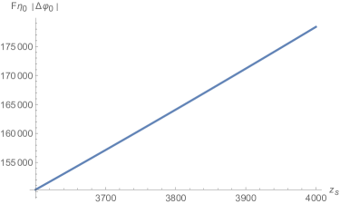
Figure 2: The polarization angle $\left|\Delta\varphi_{0}\right|$ is a function of the redshift $z_{s}$ in the radiation-dominated epoch, and we set $3600\leq z_{s}\leq 4000$.

III.2 Matter-Dominated Epoch

In the matter-dominated epoch, we have $a=({\eta}/{\eta_{0}})^{2}$ and,

$$D_{ij}^{(tail)} = \frac{4G_{N}}{\eta_{0}^{2}a^{3/2}(\eta)}\hat{D}_{ij}^{(tail)}(v),$$

$$\hat{D}_{ij}^{(tail)}(v) = \int_{0}^{v-0^{+}}{\mathrm{d}\eta^{\prime}a^{5/2}}(\eta^{\prime}){\int_{\mathbb{R}^{3}}{\mathrm{d}^{3}\vec{x}^{\prime}\Pi_{ij}\left(\eta^{\prime},\vec{x}^{\prime}\right)}}.$$

Then, from Eq.(2.2) we find that

$${\cal{T}}_{\sigma}(u,v)=\frac{{\cal{C}}_{\sigma}(v)}{a^{1/2}(\eta)},$$ (3.11)

where ${\cal{C}}_{\sigma}(v)$ is related to the source as ${\cal{C}}_{\sigma}(v)\simeq(G_{N}/\eta_{0}^{2})\hat{D}_{ij}^{(tail)}(v)$. Hence, substituting $n=\frac{3}{2}$ and in the limit $x,y<<z$ we obtain

$${\mbox{Re}}\left(\Psi_{0}\right) = -\frac{1}{4A^{2}a^{4}}\Bigg{[}\frac{1}{{\cal{R}}}\Bigg{(}{\cal{P}}_{+,vv}-\frac{2\sqrt{2}}{\eta}{\cal{P}}_{+,v}+\frac{3}{\eta^{2}}{\cal{P}}_{+}\Bigg{)}$$

$$~{}~{}+\frac{1}{a^{2}}\Bigg{(}{\cal{C}}_{+}(v)_{,vv}\frac{4\sqrt{2}}{\eta}{\cal{C}}_{+}(v)_{,v}+\frac{19}{2\eta^{2}}{\cal{C}}_{+}(v)\Bigg{)}\Bigg{]}\epsilon+{\cal{O}}\left(\epsilon^{2}\right),$$

$${\mbox{Im}}\left(\Psi_{0}\right) = \frac{1}{4A^{2}a^{4}}\Bigg{[}\frac{1}{{\cal{R}}}\Bigg{(}{\cal{P}}_{\times,vv}-\frac{2\sqrt{2}}{\eta}{\cal{P}}_{\times,v}+\frac{3}{\eta^{2}}{\cal{P}}_{\times}\Bigg{)}$$ (3.12)

$$~{}~{}+\frac{1}{a^{2}}\Bigg{(}{\cal{C}}_{\times}(v)_{,vv}\frac{4\sqrt{2}}{\eta}{\cal{C}}_{\times}(v)_{,v}+\frac{19}{2\eta^{2}}{\cal{C}}_{\times}(v)\Bigg{)}\Bigg{]}\epsilon+{\cal{O}}\left(\epsilon^{2}\right).$$

It is obvious that ${\cal{C}}(v)$ is highly suppressed by ${P_{\sigma}(v)}/{{\cal{R}}}$ while taking $\eta_{0}$ as the age of the universe, we find

$$\left|\frac{{\cal{C}}_{\sigma}(v_{0})}{P_{\sigma}(v_{0})/{\cal{R}}}\right|\simeq\frac{\Delta t}{\eta_{0}}\frac{\left|\vec{x}\right|}{\eta_{0}}a^{-3/2}(\eta_{\ast}),$$ (3.13)

where $a(\eta_{0})=1$, $\Delta t\simeq\int_{peakwidth}{d\eta a(\eta)}$, and $\eta_{\ast}$ is the peak time of the source’s strength. Then, we find

$$\varphi_{0}(u,v) = \frac{1}{2}\arctan\left(\frac{{\cal{P}}_{\times,vv}}{{\cal{P}}_{+,vv}}\right)+\frac{\sqrt{2}}{\eta}\cdot g(v)+{\cal{O}}\left(\frac{1}{\eta^{2}}\right),$$

$$\varphi_{0}(u,v)_{,u} = -\frac{1}{\eta^{2}}\cdot g(v)+{\cal{O}}\left(\frac{1}{\eta^{3}}\right).$$ (3.14)

Assume that the matter-dominated epoch is through the whole cosmic history, then the accumulation of the polarization angle from the source to the earth is given by,

$$\left|\Delta\varphi_{0}\right| \simeq \left|\sqrt{2}\left(\frac{1}{\eta_{0}}-\frac{1}{\eta_{e}}\right)\cdot g(v_{e})\right|$$

$$\simeq \left|\frac{\sqrt{2}}{\eta_{0}}\left(1-\frac{1}{\sqrt{a(\eta_{e})}}\right)\cdot g(v_{e})\right|$$

$$\simeq \left|\frac{\sqrt{2}}{\eta_{0}}\left(1-\sqrt{1+z_{s}}\right)\cdot g(v_{e})\right|.$$

Thus, the rotation angle in observer’s frame is

$$\left|\Delta\varphi_{0}\right| \simeq \left|\frac{1}{2\eta_{0}}\left(1-\sqrt{1+z_{s}}\right)\cdot\frac{(1+z_{s})^{5/8}}{F(\tau_{obs})}\right|.$$

We can also plot $\left|\Delta\varphi_{0}\right|$ as a function of $z_{s}$, which is given in Fig. 3.

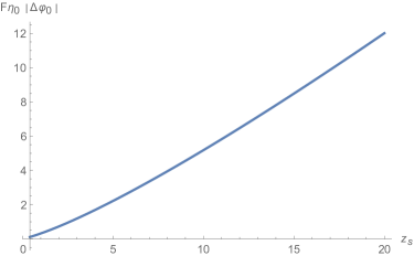
Figure 3: The polarization rotation $\left|\Delta\varphi_{0}\right|$ is a function of the redshift $z_{s}$ in the matter-dominated epoch, and we set $0.4\leq z_{s}\leq 20$ .

III.3 de Sitter Background

In this case, the tail $D_{ij}^{(tail)}(\eta,\vec{x})$ takes the form Chu15 ,

$$D_{ij}^{(tail)}(\eta,\vec{x}) = \frac{4G_{N}}{\eta_{0}^{2}}\hat{D}_{ij}^{(tail)}(v),$$

$$\hat{D}_{ij}^{(tail)}(v) \equiv \int_{-\infty}^{v-0^{+}}{\mathrm{d}\eta^{\prime}a^{4}(\eta^{\prime})}\int_{\mathbb{R}^{3}}{\mathrm{d}^{3}\vec{x}^{\prime}\Pi_{ij}\left(\eta^{\prime},\vec{x}^{\prime}\right)}.$$

In the present case, we have

$${\cal{T}}_{\sigma}=a(\eta){\cal{D}}_{\sigma}(v),$$ (3.18)

where ${\cal{D}}_{\sigma}(v)\simeq{(G_{N}/\eta_{0}^{2})}\hat{D}_{ij}^{(tail)}(v)$ is related to the integration of the source, as that given by Eq.(III.3). With $n=0$ and $a(\eta)=({\eta_{0}}/{\eta})$, from Eqs.(2.13) and (2.14), we find that

$${\mbox{Re}}\left(\Psi_{0}\right) = -\frac{1}{4A^{2}a^{4}}\Bigg{[}\frac{1}{{\cal{R}}}\Bigg{(}{\cal{P}}_{+,vv}+\frac{\sqrt{2}}{\eta}{\cal{P}}_{+,v}\Bigg{)}$$

$$~{}~{}+a\Bigg{(}{\cal{D}}_{+}(v)_{,vv}-\frac{\sqrt{2}}{\eta}{\cal{D}}_{+}(v)_{,v}+\frac{1}{2\eta^{2}}{\cal{D}}_{+}(v)\Bigg{)}\Bigg{]}\epsilon+{\cal{O}}\left(\epsilon^{2}\right),$$

$${\mbox{Im}}\left(\Psi_{0}\right) = \frac{1}{4A^{2}a^{4}}\Bigg{[}\frac{1}{{\cal{R}}}\Bigg{(}{\cal{P}}_{\times,vv}+\frac{\sqrt{2}}{\eta}{\cal{P}}_{\times,v}\Bigg{)}$$ (3.19)

$$~{}~{}+a\Bigg{(}{\cal{D}}_{\times}(v)_{,vv}-\frac{\sqrt{2}}{\eta}{\cal{D}}_{\times}(v)_{,v}+\frac{1}{2\eta^{2}}{\cal{D}}_{\times}(v)\Bigg{)}\Bigg{]}\epsilon+{\cal{O}}\left(\epsilon^{2}\right).$$

Similar to the matter-dominated case, now ${\cal{D}}_{\sigma}(v)$ is bounded by

$$\left|{\cal{D}}_{\sigma}(v)\right|\lesssim{(G_{N}/\eta_{0}^{2})}\Delta t\left|\int_{\mathbb{R}^{3}}{\mathrm{d}^{3}\vec{x}^{\prime}a^{3}(\eta_{\ast})\Pi_{ij}\left(\eta_{\ast},\vec{x}^{\prime}\right)}\right|,$$

where $\Delta t\simeq\int_{peakwidth}{d\eta a(\eta)}$, and $\eta_{\ast}$ is the peak time of the source’s strength. Then, we find that,

$$\left|\frac{{\cal{D}}_{\sigma}(v)}{P_{\sigma}(v)/{\cal{R}}}\right|\sim{(H\cdot\Delta t)\cdot(H\cdot a(\eta)\left|\vec{x}\right|)},\\$$ (3.21)

where $\eta_{0}=-\frac{1}{H}$. Substituting Eq.(III.3) into Eq.(2.21) and then carrying out the series expansion, we finally find

$$\varphi_{0}(u,v) = \frac{1}{2}\arctan\left(\frac{{\cal{P}}_{\times,vv}}{{\cal{P}}_{+,vv}}\right)-\frac{1}{\sqrt{2}\eta}\cdot g(v)+O(\frac{1}{\eta^{2}})$$

$$\varphi_{0}(u,v)_{,u} = \frac{1}{2\eta^{2}}\cdot g(v)+{\cal{O}}\left(\frac{1}{\eta^{3}}\right).$$ (3.22)

Similarly, supposing that the de sitter epoch is through the whole cosmic history, we have

$$\left|\Delta\varphi_{0}\right| \simeq \left|\frac{1}{\sqrt{2}}\Big{(}\frac{1}{\eta_{0}}-\frac{1}{\eta_{e}}\Big{)}\cdot g(v_{e})\right|$$

$$\simeq \left|\frac{1}{\sqrt{2}\eta_{0}}\Big{(}1-a(\eta_{e})\Big{)}\cdot g(v_{e})\right|$$

$$\simeq \left|\frac{1}{\sqrt{2}\eta_{0}}\Big{(}1-\frac{1}{1+z_{s}}\Big{)}\cdot g(v_{e})\right|.$$

Thus, the polarization angle in observer’s frame can be expressed as,

$$\left|\Delta\varphi_{0}\right| \simeq \frac{H}{4}\left(\frac{z_{s}}{1+z_{s}}\right)\cdot\frac{(1+z_{s})^{5/8}}{F(\tau_{obs})}.$$ (3.24)

To see this effect more explicitly, we plot $\left|\Delta\varphi_{0}\right|$ as a function of $z_{s}$ in Fig. 4.

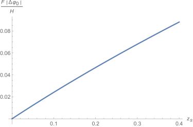
Figure 4: The polarization rotation angle $\left|\Delta\varphi_{0}\right|$ is a function of the redshift $z_{s}$ in de sitter epoch, and we set $0\leq z_{s}\leq 0.4$.

III.4 More realistic considerations

In the last subsections, we have assumed that there is only one epoch throughout the whole cosmic history. The real universe is obviously not the case. In this subsection, we will consider a more realistic case by combining all these epochs together within the framework of the $\Lambda$CDM model. We consider a binary system emitted GW signals at some time $\eta_{e}$. Then, we should integrate the polarization rotations from $\eta_{e}$ to $\eta_{\Lambda}$, the receiving time of detectors. The whole picture is sketched in Fig. 5.

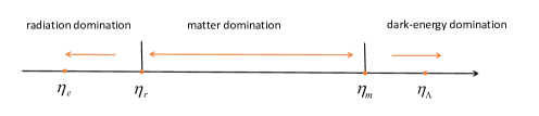
Figure 5: Sketch of propagations of GWs in the evoluated universe. $\eta_{e}$ is the emission time of the GWs, $\eta_{r}$ denotes the time when radiation-domination is ended, $\eta_{m}$ denotes the time when matter-domination epoch is ended, and $\eta_{\Lambda}$ is the receiving time of the detector.

Obviously, we have

$$\eta_{e} = \int^{z_{s}}_{\infty}\frac{-\mathrm{d}z}{H_{0}\sqrt{\Omega_{\Lambda}+\Omega_{M}(1+z)^{3}+\Omega_{R}(1+z)^{4}}},$$

$$\eta_{r} = \int^{z_{r}}_{\infty}\frac{-\mathrm{d}z}{H_{0}\sqrt{\Omega_{\Lambda}+\Omega_{M}(1+z)^{3}+\Omega_{R}(1+z)^{4}}},$$

$$\eta_{m} = \int^{z_{m}}_{\infty}\frac{-\mathrm{d}z}{H_{0}\sqrt{\Omega_{\Lambda}+\Omega_{M}(1+z)^{3}+\Omega_{R}(1+z)^{4}}},$$

$$\eta_{\Lambda} = \int^{0}_{\infty}\frac{-\mathrm{d}z}{H_{0}\sqrt{\Omega_{\Lambda}+\Omega_{M}(1+z)^{3}+\Omega_{R}(1+z)^{4}}}.$$

The fucntion $g(v_{e})$ in observer’s frame is given by

$$g(v_{e}) \simeq \frac{1}{2\sqrt{2}}\frac{(1+z_{s})^{5/8}}{F(\tau_{obs})},$$

$$F(\tau_{obs}) \equiv \Big{(}\frac{5}{256}\frac{1}{\tau_{obs}}\Big{)}^{3/8}\left(G_{N}M_{c}\right)^{-5/8},$$

where $z_{s}$ is the redshift of the source at $\eta_{e}$, and $z_{r}\simeq 3600$ at $\eta_{r}$ Ryden:2003yy , $z_{m}\simeq 0.4$ at $\eta_{m}$ Ryden:2003yy . $\Omega_{\Lambda}$, $\Omega_{M}$ and $\Omega_{R}$ are the density parameters for dark energy, matter and radiation, respectively. $H_{0}$ is the Hubble constant.

Depending on the values of $z_{s}$, the total rotation angle of the whole propagation process can be divided into the following three cases.

• $0<z_{s}<0.4$, that is, $\eta_{m}<\eta_{e}<\eta_{\Lambda}$. The accumulated polarization angle from $\eta_{e}$ to $\eta_{\Lambda}$ is

  $$\left|\Delta\varphi_{0}\right| \equiv \left|\Delta\varphi_{0}\right|_{\Lambda}.$$ (3.27)

  with

  $$\left|\Delta\varphi_{0}\right|_{\Lambda} \simeq \left|\int^{\eta_{\Lambda}}_{\eta_{e}}\frac{1}{\sqrt{2}\eta^{2}}\mathrm{d}\eta\;g(v_{e})\right|,$$ (3.28)

  where $\left|\Delta\varphi_{0}\right|_{\Lambda}$ is the polarization angle from $\eta_{e}$ to $\eta_{\Lambda}$.

• $0.4<z_{s}<3600$, that is, $\eta_{r}<\eta_{e}<\eta_{m}$. The accumulated polarization angle from $\eta_{e}$ to $\eta_{\Lambda}$ is

  $$\left|\Delta\varphi_{0}\right| \equiv \left|\Delta\varphi_{0}\right|_{m}+\left|\Delta\varphi_{0}\right|_{\Lambda}.$$ (3.29)

  with

  $$\left|\Delta\varphi_{0}\right|_{m} \simeq \left|-\int^{\eta_{m}}_{\eta_{e}}\frac{\sqrt{2}}{\eta^{2}}\mathrm{d}\eta\;g(v_{e})\right|,$$

  $$\left|\Delta\varphi_{0}\right|_{\Lambda} \simeq \left|\int^{\eta_{\Lambda}}_{\eta_{m}}\frac{1}{\sqrt{2}\eta^{2}}\mathrm{d}\eta\;g(v_{e})\right|,$$ (3.30)

  where $\left|\Delta\varphi_{0}\right|_{m}$ is the polarization angle from $\eta_{e}$ to $\eta_{m}$, and $\left|\Delta\varphi_{0}\right|_{\Lambda}$ is the rotation angle from $\eta_{m}$ to $\eta_{\Lambda}$.

• $z_{s}>3600$, that is, $\eta_{e}<\eta_{r}$. The accumulated polarization angle from $\eta_{e}$ to $\eta_{\Lambda}$ is

  $$\left|\Delta\varphi_{0}\right| \equiv \left|\Delta\varphi_{0}\right|_{r}+\left|\Delta\varphi_{0}\right|_{m}+\left|\Delta\varphi_{0}\right|_{\Lambda}.$$

  with

  $$\left|\Delta\varphi_{0}\right|_{r} \simeq \left|-\frac{1}{\sqrt{2}}\int^{\eta_{r}}_{\eta_{e}}\frac{1}{\eta^{2}}\mathrm{d}\eta\;g(v_{e})\right|,$$

  $$\left|\Delta\varphi_{0}\right|_{m} \simeq \left|-\int^{\eta_{m}}_{\eta_{r}}\frac{\sqrt{2}}{\eta^{2}}\mathrm{d}\eta\;g(v_{e})\right|,$$

  $$\left|\Delta\varphi_{0}\right|_{\Lambda} \simeq \left|\int^{\eta_{\Lambda}}_{\eta_{m}}\frac{1}{\sqrt{2}\eta^{2}}\mathrm{d}\eta\;g(v_{e})\right|,$$ (3.32)

  where $\left|\Delta\varphi_{0}\right|_{r}$ is the polarization angle from $\eta_{e}$ to $\eta_{r}$, $\left|\Delta\varphi_{0}\right|_{m}$ is the polarization angle from $\eta_{r}$ to $\eta_{m}$, and $\left|\Delta\varphi_{0}\right|_{\Lambda}$ is the polarization angle from $\eta_{m}$ to $\eta_{\Lambda}$.

At the end, we use the Plank 2015 data Aghanim:2018eyx : $\Omega_{\Lambda}=0.6935$, $\Omega_{m}=0.3065$, $\Omega_{R}=0$. Thus, the accumulated polarization angle in the whole propagation process are shown in Fig. 6 and Fig. 7.

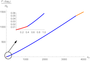
Figure 6: The polarization rotation angle $\frac{F\left|\Delta\varphi_{0}\right|}{H_{0}}$ as a function of the redshift $z_{s}$ in the whole propagation process. The red line is the first section when $0<z_{s}<0.4$, the blue line is the second section when $0.4<z_{s}<3600$, and the orange line is the third section when $3600<z_{s}<4000$.

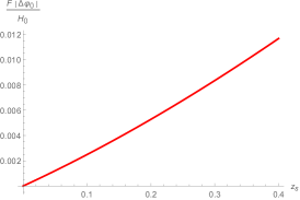
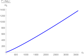
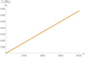
Figure 7: The rotation angle when $0<z_{s}<0.4$ (left), $0.4<z_{s}<3600$ (middle), $3600<z_{s}<4000$ (right).

To show the rotation angle more intuitively, let us consider the following two examples:

• The binary system at redshift $z_{s}=60$. The range of frequency is from $10$ Hz to $1000$ Hz.

  $$\eta_{e} = \int^{60}_{\infty}\frac{-\mathrm{d}z}{H_{0}\sqrt{\Omega_{\Lambda}+\Omega_{M}(1+z)^{3}+\Omega_{R}(1+z)^{4}}},$$ (3.33)

  $$\left|\Delta\varphi_{0}\right| \simeq \left|-\int^{\eta_{m}}_{\eta_{e}}\frac{\sqrt{2}}{\eta^{2}}\mathrm{d}\eta\;g(v_{e})\right|+\left|\int^{\eta_{\Lambda}}_{\eta_{m}}\frac{1}{\sqrt{2}\eta^{2}}\mathrm{d}\eta\;g(v_{e})\right|$$ (3.34)

  $$\simeq 0.2925H_{0}/f^{(obs)}_{gw}.$$

  We plot $\Delta\varphi_{0}$ as a function of frequency $f^{(obs)}_{gw}$ in Fig. 8 where the source redshift is $z_{s}=60$.

• The binary system at redshift $z_{s}=10$. The range of frequency is from $10^{-4}$ Hz to $10^{-2}$ Hz.

  $$\eta_{e} = \int^{10}_{\infty}\frac{-\mathrm{d}z}{H_{0}\sqrt{\Omega_{\Lambda}+\Omega_{M}(1+z)^{3}+\Omega_{R}(1+z)^{4}}},$$ (3.35)

  $$\left|\Delta\varphi_{0}\right| \simeq \left|-\int^{\eta_{m}}_{\eta_{e}}\frac{\sqrt{2}}{\eta^{2}}\mathrm{d}\eta\;g(v_{e})\right|+\left|\int^{\eta_{\Lambda}}_{\eta_{m}}\frac{1}{\sqrt{2}\eta^{2}}\mathrm{d}\eta\;g(v_{e})\right|$$ (3.36)

  $$\simeq 0.0945461H_{0}/f^{(obs)}_{gw}.$$

  We plot $\Delta\varphi_{0}$ as a function of frequency $f^{(obs)}_{gw}$ in Fig. 8 where the source redshift is $z_{s}=10$.

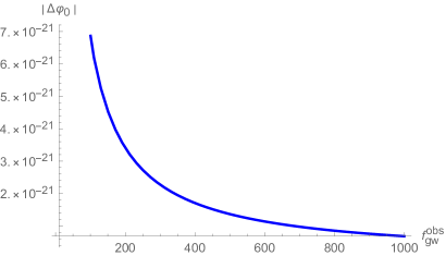
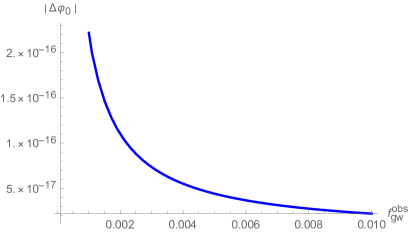
Figure 8: The rotation angle $\Delta\varphi_{0}$ is the function of frequency $f^{(obs)}_{gw}$ when we have a given source redshift. The left panel shows the rotation angle $\Delta\varphi_{0}$ in the case that redshift $z_{s}=60$ and frequency $10$ Hz - $1000$ Hz (left). The right panel shows the rotation angle $\Delta\varphi_{0}$ in the case that redshift $z_{s}=10$ and frequency $10^{-4}$ Hz - $10^{-2}$ Hz (right). Here, we set $H_{0}=70~{}km/s/\mathrm{M}pc$.

From these quantitative estimates, one can conclude that the value of $|\Delta\varphi|$ is very small, far from the sensitivity of the existing ground-based laser interferometers like LIGO and Virgo. Moreover, the lower the frequency, the more obvious the rotation of the polarization. Hence, it is possible to observe this effect for future GW detectors in extremely low frequency.

IV Conclusion and Discussion

In this paper, we have carried out the detailed analysis on the polarizations of a GW emitted by an astrophysical source at a cosmic scale distance and propagating through the flat FLRW background to the Earth. In such a curved background, GWs usually consist of two different parts, the direct and tail. To define the polarization of such a GW, we have first studied the null geodesic deviations and written them in terms of the Weyl and Ricci scalars, $\Psi_{A}$ and $\Phi_{AB}$, the projections of the Weyl tensor and Ricci tensor onto a null tetrad, as the latter have direct physical meaning, which enable us to define the polarization of a GW, given, respectively, by Eqs.(2.21) and (2.27), in terms of the real and imaginary parts of the Weyl scalars, $\Psi_{0}$ and $\Psi_{4}$. Since the two spatial unit vectors $e_{2}$ and $e_{3}$, which span the polarization plane of the GW, are parallel-transported along the null geodesics, the change of the polarization angle is gauge-invariant, that is, if the polarization angle changes in one coordinate system, it will change in any of them. After detailed analyses, we have shown that effects of the expanding universe on the “+” and “$\times$” modes are different, and usually depend on their waveforms. As a result, the polarization angle gets changed when the wave propagates through our Universe. In particular, we have found that in different epochs of the universe, the effects are also different. For a GW emitted by a binary system, we have found explicitly the relation between the change of the polarization angle $|\Delta\varphi|$ and the redshift $z_{s}$ of the source in different epochs. In particular, in the standard $\Lambda$CDM model, we have shown that the order of $|\Delta\varphi|{\eta_{0}F}$ is typically $O(10^{-3})$ to $O(10^{3})$, depending on the values of $z_{s}$, where $\eta_{0}$ is the (comoving) time of the current universe, and $F\equiv\Big{(}\frac{5}{256}\frac{1}{\tau_{obs}}\Big{)}^{3/8}\left(G_{N}M_{c}\right)^{-5/8}$ with $\tau_{obs}$ and $M_{c}$ being, respectively, the time to coalescence in the observer’s frame and the chirp mass of the binary system. Particularly, for typical sources of LIGO/Virgo, we find the typical value for $|\Delta\varphi|$ is $10^{-21}$ as shown in Fig. (8), which is very small and is far from being detected by the current detectors. However, for lower frequency, the observation effect increases linearly. Hence, it is possible for future GW detectors sensitive in extremely low frequency.

It should be noted that there are two timescales: One is related to the propagation of GWs, the other refers to the period of detections of GWs. The former can be comparable with the age of the universe for astrophysical GW sources with high redshift, while the latter is of the order of seconds for the current ground-based detectors. Therefore, the changes of polarizations of GWs cannot be directly related to the current detections of GWs. However, the effects of the background on the propagations and polarizations of such GWs cannot be ignored as shown in section III, especially for sources with low frequency and high redshift.

It would be very interesting to find the observational signature of the rotations of the polarization. However, since the changes are due to the curvature of the background, they become significant only over cosmic scales. Therefore, to detect such effects, combinations of cosmic distant objects with the ground- and/or space-based detectors might be needed. Interestingly, analysis about the amplitude and phase of GWs traveling a long cosmological distance has been discussed a lot in Hou:2019jhu .

In addition, in this paper we assumed that the GWs are propagating on the homogeneous and isotropic background. This implies that the wavelengths of such GWs are much shorter than the scale, over which the changes of the universe including its perturbations are negligible. This automatically ignores the gravitational lensing of such GWs by massive objects, such as galaxies and supermassive black holes. It would be very interesting and important to study such effects, specially their observational evidences.

Appendix A The Weyl, Ricci Scalars and Gauge Invariance

In this appendix, we present some detailed computations of the Weyl and Ricci scalars in terms of the null tetrad. In particular, we find,

$$\Psi_{0} \equiv -C_{\mu\nu\lambda\delta}l^{\mu}m^{\nu}l^{\lambda}m^{\delta}$$

$$= {-}\frac{1}{8A^{2}a^{4}}\big{[}-2h_{+,\eta z}+h_{+,zz}+h_{+,\eta\eta}-i(-2h_{{\times},\eta z}+h_{{\times},zz}+h_{{\times},\eta\eta})\big{]}\epsilon+O(\epsilon^{2}),$$

$$\Psi_{1} \equiv -C_{\mu\nu\lambda\delta}l^{\mu}n^{\nu}l^{\lambda}m^{\delta}$$

$$= {-}\frac{\sqrt{2}}{16a^{3}A}\big{[}h_{+,\eta x}-h_{+,xz}+i(h_{+,yz}-h_{+,\eta y})-i(h_{{\times},\eta x}-h_{{\times},xz}+i(h_{{\times},yz}-h_{{\times},\eta y}))\big{]}\epsilon+O(\epsilon^{2}),$$

$$\Psi_{2} \equiv -\frac{1}{2}C_{\mu\nu\lambda\delta}\big{(}l^{\mu}n^{\nu}l^{\lambda}n^{\delta}-l^{\mu}n^{\nu}m^{\lambda}\bar{m}^{\delta}\big{)}$$

$$= {-}\frac{1}{12a^{2}}\big{(}h_{+,xx}-h_{+,yy}-2h_{{\times},xy}\big{)}\epsilon+O(\epsilon^{2}),$$

$$\Psi_{3} \equiv {-}C_{\mu\nu\lambda\delta}l^{\mu}n^{\nu}n^{\lambda}\bar{m}^{\delta}$$

$$= {-}\frac{\sqrt{2}A}{8a}\big{[}h_{+,\eta x}+h_{+,xz}+i(h_{+,yz}+h_{+,\eta y})+i(h_{{\times},\eta x}+h_{{\times},xz}+i(h_{{\times},yz}+h_{{\times},\eta y}))\big{]}\epsilon+O(\epsilon^{2}),$$

$$\Psi_{4} \equiv -C_{\mu\nu\lambda\delta}n^{\mu}\bar{m}^{\nu}n^{\lambda}\bar{m}^{\delta}$$

$$= {-}\frac{A^{2}}{2}\big{[}2h_{+,\eta z}+h_{+,zz}+h_{+,\eta\eta}+i(2h_{{\times},\eta z}+h_{{\times},zz}+h_{{\times},\eta\eta})\big{]}\epsilon+O(\epsilon^{2}),$$

and

$$\Phi_{00} \equiv {-}\frac{1}{2}S_{\mu\nu}l^{\mu}l^{\nu}$$

$$= \frac{1}{4A^{2}a^{6}}\big{(}2{a^{\prime}}^{2}-aa^{\prime\prime}\big{)}+O\left(\epsilon^{2}\right),$$

$$\Phi_{11} \equiv {-}\frac{1}{4}S_{\mu\nu}(l^{\mu}n^{\nu}+m^{\mu}\bar{m}^{\nu})$$

$$= \frac{1}{4a^{4}}\big{(}2{a^{\prime}}^{2}-aa^{\prime\prime}\big{)}{-}\frac{1}{8a^{2}}\big{(}h_{+,yy}-h_{+,xx}+2h_{{\times},yx}\big{)}\epsilon+O(\epsilon^{2}),$$

$$\Phi_{22} \equiv {-}\frac{1}{2}S_{\mu\nu}n^{\mu}n^{\nu}$$

$$= \frac{A^{2}}{a^{2}}\big{(}2{a^{\prime}}^{2}-aa^{\prime\prime}\big{)}+O(\epsilon^{2}),$$

$$\Phi_{01} \equiv {-}\frac{1}{2}S_{\mu\nu}l^{\mu}m^{\nu}$$

$$= {-}\frac{\sqrt{2}}{16a^{3}A}\big{[}h_{+,xz}-h_{+,\eta x}+i(h_{+,\eta y}-h_{+,yz})-i\left(h_{{\times},xz}-h_{{\times},\eta x}+i(h_{{\times},\eta y}-h_{{\times},yz})\right)\big{]}\epsilon+O(\epsilon^{2}),$$

$$\Phi_{02} \equiv {-}\frac{1}{2}S_{\mu\nu}m^{\mu}m^{\nu}$$

$$= {-}\frac{1}{4a^{3}}\big{[}a(h_{+,zz}-h_{+,\eta\eta})-2a^{\prime}h_{+,\eta}-i\left(a(h_{{\times},zz}-h_{{\times},\eta\eta})-2a^{\prime}h_{{\times},\eta}\right)\big{]}\epsilon+O(\epsilon^{2}),$$

$$\Phi_{12} \equiv {-}\frac{1}{2}S_{\mu\nu}n^{\mu}n^{\nu}$$

$$= {-}\frac{\sqrt{2}A}{8a}\big{[}-h_{+,xz}-h_{+,\eta x}+i(h_{+,\eta y}+h_{+,yz})-i\left(-h_{{\times},xz}-h_{{\times},\eta x}+i(h_{{\times},\eta y}+h_{{\times},yz})\right)\big{]}\epsilon+O(\epsilon^{2}),$$

$$\Phi_{\Lambda} \equiv {+}\frac{R}{24}$$ (A.38)

$$= \frac{a^{\prime\prime}}{4a^{3}}{-}\frac{1}{24a^{2}}\big{(}h_{+,yy}-h_{+,xx}+2h_{{\times},xy}\big{)}\epsilon+O(\epsilon^{2}).$$

When $\mid z\mid\gg x$ and $\mid z\mid\gg y$, we find,

$$\mid\vec{x}\mid = z+\frac{x^{2}+y^{2}}{2z}+O\left(\frac{1}{z^{3}}\right),\quad v={\frac{1}{\sqrt{2}}}(\eta-\mid\vec{x}\mid)={\frac{1}{\sqrt{2}}}\Bigg{(}\eta-z-\frac{x^{2}+y^{2}}{2z}+O\left(\frac{1}{z^{3}}\right)\Bigg{)},$$

$$\cal{R} = a(\eta)\mid\vec{x}\mid=a\left(z+\frac{x^{2}+y^{2}}{2z}\right)+O\left(\frac{1}{z^{3}}\right).$$ (A.39)

Then from (2.2) we obtain

$$h_{\sigma,\eta\eta} = \frac{1}{\cal{R}}\Bigg{[}\frac{1}{2}{{\cal{P}}_{{\sigma},vv}}-\sqrt{2}{{\cal{H}}}{{\cal{P}}_{\sigma,v}}+\Big{(}{{\cal{H}}}^{2}-{{\cal{H}^{\prime}}}\Big{)}{{\cal{P}}_{\sigma}}\Bigg{]}+\frac{1}{a^{n}}\Bigg{[}{\frac{1}{2}{\cal{T}}_{\sigma,uu}}+\frac{1}{2}{{\cal{T}}_{\sigma,vv}}-\sqrt{2}n{{\cal{H}}}({{\cal{T}}_{\sigma,u}}+{{\cal{T}}_{\sigma,v}})$$

$$~{}~{}~{}~{}~{}~{}~{}~{}+n(n{{\cal{H}}}^{2}-{{\cal{H}^{\prime}}}){{\cal{T}}_{\sigma}}\Bigg{]},$$

$$h_{\sigma,\eta x} = \frac{1}{{\cal{R}}z}\Bigg{(}-\frac{1}{2}{\cal{P}}_{{\sigma},vv}+\frac{1}{\sqrt{2}}{\cal{H}}{\cal{P}}_{\sigma,v}\Bigg{)}x+\frac{1}{a^{n}}\Bigg{[}{\frac{1}{2}{\cal{T}}_{\sigma,uu}}-\frac{1}{2}{{\cal{T}}_{\sigma,vv}}-\frac{1}{\sqrt{2}}n{{\cal{H}}}({{\cal{T}}_{\sigma,u}}-{{\cal{T}}_{\sigma,v}})\Bigg{]}\frac{x}{z}+O\left(\frac{1}{z^{3}}\right),$$

$$h_{\sigma,\eta y} = \frac{1}{{\cal{R}}z}\Bigg{(}-\frac{1}{2}{\cal{P}}_{{\sigma},vv}+\frac{1}{\sqrt{2}}{\cal{H}}{\cal{P}}_{\sigma,v}\Bigg{)}y+\frac{1}{a^{n}}\Bigg{[}{\frac{1}{2}{\cal{T}}_{\sigma,uu}}-\frac{1}{2}{{\cal{T}}_{\sigma,vv}}-\frac{1}{\sqrt{2}}n{{\cal{H}}}({{\cal{T}}_{\sigma,u}}-{{\cal{T}}_{\sigma,v}})\Bigg{]}\frac{y}{z}+O\left(\frac{1}{z^{3}}\right),$$

$$h_{\sigma,\eta z} = -\frac{1}{2}\frac{{\cal{P}}_{{\sigma},vv}}{{\cal{R}}}+\frac{1}{\sqrt{2}}\left({\cal{H}}-\frac{a}{{\cal{R}}}\right)\frac{{\cal{P}}_{\sigma,v}}{{\cal{R}}}+a{\cal{H}}\frac{{\cal{P}}_{\sigma}}{{\cal{R}}^{2}}+\frac{1}{a^{n}}\Bigg{[}\frac{1}{2}{{\cal{T}}_{\sigma,uu}}-\frac{1}{2}{{\cal{T}}_{\sigma,vv}}-\frac{1}{\sqrt{2}}n{{\cal{H}}}({{\cal{T}}_{\sigma,u}}-{{\cal{T}}_{\sigma,v}})\Bigg{]}$$

$$\times\left(1-\frac{x^{2}+y^{2}}{2z^{2}}\right)+O\left(\frac{1}{z^{3}}\right),$$

$$h_{\sigma,xx} = -\frac{1}{\sqrt{2}}\frac{{\cal{P}}_{\sigma,v}}{{\cal{R}}z}+\frac{1}{a^{n}}\Bigg{[}\frac{1}{2}({{\cal{T}}_{\sigma,uu}}+{{\cal{T}}_{\sigma,vv}})\frac{x^{2}}{z^{2}}+\frac{1}{\sqrt{2}}({{\cal{T}}_{\sigma,u}}-{{\cal{T}}_{\sigma,v}})\frac{1}{z}\Bigg{]}+O\left(\frac{1}{z^{3}}\right),$$

$$h_{\sigma,yy} = -\frac{1}{\sqrt{2}}\frac{{\cal{P}}_{\sigma,v}}{{\cal{R}}z}+\frac{1}{a^{n}}\Bigg{[}\frac{1}{2}({{\cal{T}}_{\sigma,uu}}+{{\cal{T}}_{\sigma,vv}})\frac{y^{2}}{z^{2}}+\frac{1}{\sqrt{2}}({{\cal{T}}_{\sigma,u}}-{{\cal{T}}_{\sigma,v}})\frac{1}{z}\Bigg{]}+O\left(\frac{1}{z^{3}}\right),$$

$$h_{\sigma,zz} = \frac{1}{2}\frac{{\cal{P}}_{{\sigma},vv}}{{\cal{R}}}+\frac{\sqrt{2}a{\cal{P}}_{\sigma,v}}{{\cal{R}}^{2}}+\frac{1}{a^{n}}\left(\frac{1}{2}{{\cal{T}}_{\sigma,uu}}+\frac{1}{2}{{\cal{T}}_{\sigma,vv}}\right)\left(1-\frac{x^{2}+y^{2}}{z^{2}}\right)+O\left(\frac{1}{z^{3}}\right),$$

$$h_{\sigma,xz} = \frac{1}{2}\frac{{\cal{P}}_{{\sigma},vv}}{{\cal{R}}z}x+\frac{1}{a^{n}}\Bigg{[}\frac{1}{2}({{\cal{T}}_{\sigma,uu}}+{{\cal{T}}_{\sigma,vv}})\frac{x}{z}+\frac{1}{\sqrt{2}}({{\cal{T}}_{\sigma,v}}-{{\cal{T}}_{\sigma,u}})\frac{x}{z^{2}}\Bigg{]}+O\left(\frac{1}{z^{3}}\right),$$

$$h_{\sigma,yz} = \frac{1}{2}\frac{{\cal{P}}_{{\sigma},vv}}{{\cal{R}}z}y+\frac{1}{a^{n}}\Bigg{[}\frac{1}{2}({{\cal{T}}_{\sigma,uu}}+{{\cal{T}}_{\sigma,vv}})\frac{y}{z}+\frac{1}{\sqrt{2}}({{\cal{T}}_{\sigma,v}}-{{\cal{T}}_{\sigma,u}})\frac{y}{z^{2}}\Bigg{]}+O\left(\frac{1}{z^{3}}\right).$$ (A.40)

Inserting them into Eqs.(A) and (A), we get Eqs.(2.13), (2.14) and

$${\mbox{Re}}\left(\Phi_{02}\right) = {-}\frac{1}{4a^{2}}\Bigg{\{}\frac{1}{{\cal{R}}}\Big{[}({{\cal{H}}}^{2}+{{\cal{H}^{\prime}}}){{\cal{P}}_{+}}\Big{]}+\frac{1}{a^{n}}\Bigg{[}\frac{1}{2}\left({{\cal{T}}_{+,uu}}+{{\cal{T}}_{+,vv}}\right)\left(-\frac{x^{2}+y^{2}}{z^{2}}\right)+\sqrt{2}n{{\cal{H}}}({{\cal{T}}_{+,u}}+{{\cal{T}}_{+,v}})~{}~{}~{}~{}$$ (A.41)

$$~{}~{}~{}~{}~{}~{}~{}~{}~{}~{}~{}~{}~{}~{}-n(n{{\cal{H}}}^{2}-{{\cal{H}^{\prime}}}){{\cal{T}}_{+}}-\sqrt{2}{{\cal{H}}}({{\cal{T}}_{+,u}}+{{\cal{T}}_{+,v}})+2n{{\cal{H}}}^{2}{{\cal{T}}_{+}}\Bigg{]}\Bigg{\}}\epsilon+{\cal{O}}\left(\epsilon^{2}\right),$$

$${\mbox{Im}}\left(\Phi_{02}\right) = \frac{1}{4a^{2}}\Bigg{\{}\frac{1}{{\cal{R}}}\Big{[}({{\cal{H}}}^{2}+{{\cal{H}^{\prime}}}){{\cal{P}}_{\times}}\Big{]}+\frac{1}{a^{n}}\Bigg{[}\frac{1}{2}\left({{\cal{T}}_{\times,uu}}+{{\cal{T}}_{\times,vv}}\right)\left(-\frac{x^{2}+y^{2}}{z^{2}}\right)+\sqrt{2}n{{\cal{H}}}({{\cal{T}}_{\times,u}}+{{\cal{T}}_{\times,v}})~{}~{}~{}~{}$$ (A.42)

$$~{}~{}~{}~{}~{}~{}~{}~{}~{}~{}~{}~{}-n(n{{\cal{H}}}^{2}-{{\cal{H}^{\prime}}}){{\cal{T}}_{\times}}-\sqrt{2}{{\cal{H}}}({{\cal{T}}_{\times,u}}+{{\cal{T}}_{\times,v}})+2n{{\cal{H}}}^{2}{{\cal{T}}_{\times}}\Bigg{]}\Bigg{\}}\epsilon+{\cal{O}}\left(\epsilon^{2}\right).$$

When it comes to gauge invariance, there are two kinds of gauge transformations:

• Gauge transformations of the first kind. From Eqs.(A-A), it is clear that the physical quantities such as $\Psi_{0}$ and $\Psi_{4}$ are invariant under the change of coordinate system because the equation of NP formalism just involve scalar functions. These are the so-called gauge transformations of the first kind as defined in Sachs:1964zza .

• Gauge transformations of the second kind. The gauge transformations of the second kind have been discussed in Stewart:1974uz ; Miranda:2014vaa , which are changes of the identification map, $x^{\mu}_{\mbox{\scriptsize{new}}}=x^{\mu}_{\mbox{\scriptsize{old}}}+\epsilon\xi^{\mu}$, where $\xi^{\mu}$ is an arbitrary vector field. Then, for the liner-order perturbation of a NP quantity $L$, we have $L^{(1)\mbox{\scriptsize{new}}}=L^{(1)\mbox{\scriptsize{old}}}-\epsilon L^{(1)\mbox{\scriptsize{old}}}_{,\mu}\xi^{\mu}$. As shown in Stewart:1974uz ; Miranda:2014vaa , there are three classes of infinitesimal changes in the tetrad:

  $$\begin{aligned} &\text{(i)}~{}~{}~{}l^{\mu}\rightarrow l^{\mu},m^{\mu}\rightarrow m^{\mu}+\epsilon al^{\mu},n^{\mu}\rightarrow n^{\mu}+\epsilon\bar{a}m^{\mu}+\epsilon a\bar{m}^{\mu}+\epsilon^{2}a\bar{a}l^{\mu};\\ &\text{(ii)}~{}~{}~{}n^{\mu}\rightarrow n^{\mu},m^{\mu}\rightarrow m^{\mu}+\epsilon bn^{\mu},l^{\mu}\rightarrow l^{\mu}+\epsilon\bar{b}m^{\mu}+\epsilon b\bar{m}^{\mu}+\epsilon^{2}b\bar{b}n^{\mu};\\ &\text{(iii)}~{}~{}~{}l^{\mu}\rightarrow Al^{\mu},n^{\mu}\rightarrow A^{-1}n^{\mu},m^{\mu}\rightarrow e^{i\theta}m^{\mu},\end{aligned}$$ (A.43)

  where $a$ and $b$ are complex functions and $A$ and $\theta$ are real functions. The components of the Weyl tensor, $\Psi_{1},\Psi_{2},\Psi_{3}$ and $\Psi_{4}$, can be expressed in terms of twelve spin coefficients Griffiths76a ; Griffiths:1991zp ; NP62 . Let us take the class (i) as an example, then we find that the spin coefficients Griffiths76a ; Griffiths:1991zp ; NP62 transform as

  $$\kappa\rightarrow\kappa,\;\sigma\rightarrow\sigma+\epsilon a\kappa,\;\rho\rightarrow\rho+\epsilon\bar{a}\kappa,\;\varepsilon\rightarrow\varepsilon+\epsilon\bar{a}\kappa,$$

  $$\tau\rightarrow\tau+\epsilon a\rho+\epsilon\bar{a}\sigma+\epsilon^{2}a\bar{a}\kappa,\;\pi\rightarrow\pi+\epsilon D\bar{a}+2\epsilon\bar{a}\varepsilon+\epsilon^{2}(\bar{a})^{2}\kappa,$$

  $$\alpha\rightarrow\alpha+\epsilon\bar{a}(\rho+\varepsilon)+\epsilon^{2}(\bar{a})^{2}\kappa,\;\beta\rightarrow\beta+\epsilon a\varepsilon+\epsilon\bar{a}\sigma+\epsilon^{2}a\bar{a}\kappa,$$

  $$\gamma\rightarrow\gamma+\epsilon a\alpha+\epsilon\bar{a}(\beta+\tau)+\epsilon^{2}a\bar{a}(\rho+\varepsilon)+\epsilon^{3}(\bar{a})^{2}\sigma+\epsilon^{3}a(\bar{a})^{2}\kappa,$$

  $$\lambda\rightarrow\lambda+\epsilon\bar{a}(2\alpha+\pi)+\epsilon^{2}(\bar{a})^{2}(\rho+2\varepsilon)+\epsilon^{3}(\bar{a})^{3}\kappa+\epsilon\bar{\delta}\bar{a}+\epsilon^{2}\bar{a}D\bar{a},$$

  $$\mu\rightarrow\mu+\epsilon a\pi+2\epsilon\bar{a}\beta+2\epsilon^{2}a\bar{a}\varepsilon+\epsilon^{2}(\bar{a})^{2}\sigma+\epsilon^{3}a(\bar{a})^{2}\kappa+\epsilon\delta\bar{a}+\epsilon^{2}aD\bar{a},$$

  $$\nu\rightarrow\nu+\epsilon a\lambda+\epsilon\bar{a}(\mu+2\gamma)+\epsilon^{2}(\bar{a})^{2}(\tau+2\beta)+\epsilon^{3}(\bar{a})^{3}\sigma+\epsilon^{2}a\bar{a}(\pi+2\alpha)$$

  $$\;\;\>\quad+\epsilon^{3}a(\bar{a})^{2}(\rho+2\varepsilon)+\epsilon^{4}a(\bar{a})^{3}\kappa+\epsilon\big{(}\Delta+\epsilon\bar{a}\delta+\epsilon a\bar{\delta}+\epsilon^{2}a\bar{a}D\big{)}\bar{a}.$$ (A.44)

  Thus, $\Psi_{0},\Psi_{1},\Psi_{2},\Psi_{3}$ and $\Psi_{4}$ under the transformation transfer as

  $$\begin{aligned} &\Psi_{0}\rightarrow\Psi_{0},\;\Psi_{1}\rightarrow\Psi_{1}+\epsilon\bar{a}\Psi_{0},\;\Psi_{2}\rightarrow\Psi_{2}+2\epsilon\bar{a}\Psi_{1}+\epsilon^{2}(\bar{a})^{2}\Psi_{0},\\ &\Psi_{3}\rightarrow\Psi_{3}+3\epsilon\bar{a}\Psi_{2}+3\epsilon^{2}(\bar{a})^{2}\Psi_{1}+\epsilon^{3}(\bar{a})^{3}\Psi_{0},\\ &\Psi_{4}\rightarrow\Psi_{4}+4\epsilon\bar{a}\Psi_{3}+6\epsilon^{2}(\bar{a})^{2}\Psi_{2}+4\epsilon^{3}(\bar{a})^{3}\Psi_{1}+\epsilon^{4}(\bar{a})^{4}\Psi_{0}.\\ \end{aligned}$$ (A.45)

  Meanwhile, we find that $\Psi_{1},\Psi_{2},\Psi_{3}$ in Eqs.(A) vanish for the metric of Eq.(2.5) in the propagation region far from the source, $\left|\vec{x}\right|\gg D$, so the effect to the linear order of $\epsilon$ of $\Psi_{0}$ and $\Psi_{4}$ is

  $$\Psi_{0}^{\scriptscriptstyle{(1)}}\rightarrow\Psi_{0}^{\scriptscriptstyle{(1)}},\quad\Psi_{4}^{\scriptscriptstyle{(1)}}\rightarrow\Psi_{4}^{\scriptscriptstyle{(1)}}.$$ (A.46)

  Other classes can be studied by following similar considerations, and we find that the results are the same, so we do not show the detail here.

In summary, $\Psi_{0}$ and $\Psi_{4}$ are invariant under any kind of the gauge transformations.

Appendix B Parallel-transported Polarization Angle

It was shown in Wang91 that the above definition of the polarization angle is in general not parallel-transported along the wave paths. This makes it impossible to compare the polarization of a gravitational wave at two different points along its propagation path. One way to overcome this difficulty is to find a parallel-transported basis carried by the wave. Once we have this basis, polarization angle defined based on this basis should be parallel-transported. As suggested in Wang91 , a parallel-transported basis can be found by rotating the coordinate with a proper angle in the $(e_{2}^{\mu},e_{3}^{\mu})$ plane. Similar considerations can be generalized to the current case. In particular, for GWs along the null geodesics defined by $n^{\mu}$, we let $\varphi_{0}^{(0)}$ be the angle of rotating, and $\lambda_{(2)}^{\mu}$ and $\lambda_{(3)}^{\mu}$ be the new basis. Then, we find

$$\lambda_{(2)}^{\mu}{}_{;\nu}l^{\nu} = \left(\frac{1}{2}\sinh{W}V_{,\nu}-\varphi_{0,\nu}^{(0)}\right)l^{\nu}\lambda_{(3)}^{\mu},$$ (B.1)

$$\lambda_{(3)}^{\mu}{}_{;\nu}l^{\nu} = -\left(\frac{1}{2}\sinh{W}V_{,\nu}-\varphi_{0,\nu}^{(0)}\right)l^{\nu}\lambda_{(2)}^{\mu},$$ (B.2)

which implies

$$\varphi_{0,\nu}^{(0)}=\frac{1}{2}\sinh{W}V_{,\nu}=\epsilon^{2}h_{\times}h_{+,\nu}+\mathcal{O}(\epsilon^{3}).$$ (B.3)

Then, the angle

$$\psi_{0}\equiv\hat{\varphi}_{0}-\varphi_{0}^{(0)},$$ (B.4)

determines the polarization direction of the $\Psi_{0}$ wave relative to the $(\lambda_{(2)}^{\mu},\lambda_{(3)}^{\mu})$ basis. Similarly, for the $\Psi_{4}$ wave, the related angle is given by

$$\varphi_{4,\nu}^{(0)}=\epsilon^{2}h_{\times}h_{+,\nu}+\mathcal{O}(\epsilon^{3}),$$ (B.5)

and $\psi_{4}\equiv\hat{\varphi}_{4}-\varphi_{4}^{(0)}$ defines the angle between the polarization direction of the wave and the $\lambda_{(2)}^{\mu}$ axis. It should be noted that both $\varphi_{0}^{(0)}$ and $\varphi_{4}^{(0)}$ are $\epsilon^{2}$-term, which implies that there is no linear-order corrections.

Appendix C Timelike Geodesics Deviations and Polarization of a Gravitational Wave

In this appendix, let us consider timelike geodesic deviations, as they are directly related to observations. To our purpose, in the following we consider timelike geodesic congruences formed by $t^{\mu}$, from Eqs.(II.1) we find

$$t^{\mu}{}_{;\nu}t^{\nu}=-\frac{1}{\sqrt{2}}\left(\frac{AB_{,\eta}}{B}-\frac{BA_{,\eta}}{A}\right)s^{\mu}.$$ (C.1)

Therefore, choosing $A$ and $B$ so that

$$\frac{AB_{,\eta}}{B}-\frac{BA_{,\eta}}{A}=0,$$ (C.2)

we find $t^{\mu}{}_{;\nu}t^{\nu}=0$, that is, $t^{\mu}$ defines a timelike and affinely parametrized geodesic congruence. Recall that $2AB=a^{-2}$. Thus, the general solution of the above equation is

$$A=\frac{-A_{0}\pm\sqrt{A_{0}^{2}+2a^{2}}}{-2a^{2}},\quad B=\frac{1}{2Aa^{2}},$$ (C.3)

where $A_{0}$ is an integration constant. Without loss of the generality, we can always choose $A_{0}=0$, so that

$$A=B=\pm\frac{1}{\sqrt{2}\;a}.$$ (C.4)

In what follows, we shall adopt the “+” sign.

On the other hand, the four spatial unity vectors we constructed in section II, form an orthogonal base. Thus, the component $\Psi_{0}$ ($\Psi_{4}$) represents the GW moving along the positive (negative) $s^{\mu}$-direction, as shown in Fig. 1.

Let $\eta^{\mu}$ be the geodesic deviation between two neighbor geodesics and $\eta^{\mu}t_{\mu}=0$. Then, the timelike geodesic deviation is given by,

$$\frac{d^{2}\eta^{\mu}}{d\lambda^{2}} = -R^{\mu}_{\nu\lambda\beta}t^{\nu}\eta^{\lambda}t^{\beta}$$ (C.5)

$$= \frac{1}{2}\Big{\{}-\left(\Phi_{00}+2\Phi_{11}+\Phi_{22}-6\Phi_{\Lambda}\right)e^{\mu\nu}_{o}$$

$$+\Big{[}\left(\Psi_{2}+\bar{\Psi}_{2}\right)+2\left(\Phi_{\Lambda}-\Phi_{11}\right)\Big{]}\left(2s^{\mu}s^{\nu}-e^{\mu\nu}_{0}\right)$$

$${+}{2}{\mbox{Re}}\Big{[}\left(\Psi_{1}+\Psi_{3}\right)-\left(\Phi_{01}-\Phi_{12}\right)\Big{]}e^{\mu\nu}_{\times 2s}$$

$${+}2{\mbox{Im}}\Big{[}\left(\Psi_{1}-\Psi_{3}\right)-\left(\Phi_{01}-\Phi_{12}\right)\Big{]}e^{\mu\nu}_{\times 3s}$$

$${+}{\mbox{Re}}\left(\Psi_{0}+\Psi_{4}+2\Phi_{02}\right)\;e^{\mu\nu}_{+}$$

$$+{\mbox{Im}}\left(\Psi_{0}-\Psi_{4}+2\Phi_{02}\right)\;e^{\mu\nu}_{\times}\Big{\}}\eta_{\nu},$$

where

$$e^{\mu\nu}_{\times 2s} \equiv e^{\mu}_{2}s^{\nu}+e^{\nu}_{2}s^{\mu},\quad e^{\mu\nu}_{\times 3s}\equiv e^{\mu}_{3}s^{\nu}+e^{\nu}_{3}s^{\mu},$$

The right hand side of Eq.(C.5) includes six terms, each of them represents a sort of polarization mode, and has the following physical interpretations Szekeres65 ; WThesis . The first terms is transverse, laying on the ($e_{2},e_{3}$)-plane only, and makes the test particles contract or expand uniformly, depending on sign of the coefficient. It is remarkable to note that the Weyl scalars have no contributions to this term. The second term has the effect of distorting a sphere of particles about the observer into an ellipsoid, which has $s^{\mu}$ as principal axis, while in the perpendicular ($e_{2},e_{3}$)-plane it is uniformly contracting or expanding, depending the signs of the coefficient, $\left(\Psi_{2}+\bar{\Psi}_{2}\right)+2\left(\Phi_{\Lambda}-\Phi_{11}\right)$. This is a behavior quite similar to particles falling in towards a central attracting body with the inverse square law, so it is often to call this term as the Coulomb part of the field, and the strength of the Coulomb field of the pure gravitational field is given by the real part of $\Psi_{2}$, while the strength of the matter field is represented by $\left(\Phi_{\Lambda}-\Phi_{11}\right)$. The third term represents a force that acts only on the ($e^{\mu}_{2},s^{\mu}$)-plane. Recall $s^{\mu}$ represents the direction of the propagation of the two GW components, represented by $\Psi_{0}$ and $\Psi_{4}$, respectively, so this term is often called the longitudinal component. Rotating this plane by $45^{0}$,

$$s^{\mu} = \cos 45^{0}{s^{\prime}}^{\mu}+\sin 45^{0}{e^{\prime}}^{\mu}_{2},$$

$$e^{\mu}_{2} = -\sin 45^{0}{s^{\prime}}^{\mu}+\cos 45^{0}{e^{\prime}}^{\mu}_{2},$$ (C.7)

we find that

$$e^{\mu\nu}_{\times 2s}=-\left({s^{\prime}}^{\mu}{s^{\prime}}^{\nu}-{e^{\prime}}^{\mu}_{2}{e^{\prime}}^{\nu}_{2}\right).$$ (C.8)

Therefore, if it is initially a circle in the ($e^{\mu}_{2},s^{\mu}$)-plane, this term will make the circle into an ellipse with its major axis along the $45^{0}$ with respect to the $s^{\mu}$-direction. The strength of this force depends on the real part of the combination, $\left(\Psi_{1}+\Psi_{3}\right)-\left(\Phi_{01}-\Phi_{12}\right)$.

In contrast to the third term, the fourth term represents a force that acts only on the ($e^{\mu}_{3},s^{\mu}$)-plane, and the strength of this term depends on the imaginary part of the combination, $\left(\Psi_{1}-\Psi_{3}\right)-\left(\Phi_{01}-\Phi_{12}\right)$. Note the difference between this term and the last one in the pure gravitational part, represented by $\Psi_{1}$ and $\Psi_{3}$, respectively. In the third term, it is the real part of $\left(\Psi_{1}+\Psi_{3}\right)$, while in the fourth term, it is the imaginary part of $\left(\Psi_{1}-\Psi_{3}\right)$. This is different from the matter field, which is always proportional to the combination of $\left(\Phi_{01}-\Phi_{12}\right)$ in both terms.

The fifth term is also purely transverse and deforms a circle laying in the ($e_{2},e_{3}$)-plane into ellipse with its major axis along the $e_{2}$-direction. To see the effects of the last term, we can make a similar rotation as that given by Eq.(C) but now in the ($e_{2},e_{3}$)-plane, so we find that

$$e^{\mu\nu}_{\times}=-{e^{\prime}}^{\mu\nu}_{+}.$$ (C.9)

Therefore, the last term is also purely transverse and deforms a circle laying in the ($e_{2},e_{3}$)-plane into ellipse with its major axis along a line that has a $45^{0}$ angle with respect to the $e_{2}$-direction.

To consider the polarization of the right-moving (along the positive direction of $s^{\mu}$) GW represented by $\Psi_{0}$, let us first make the rotation as Eq.(II.1),

$$e_{2}^{\mu} = \cos\varphi_{0}\hat{e}_{2}^{\mu}+\sin\varphi_{0}\hat{e}_{3}^{\mu},$$

$$e_{3}^{\mu} = -\sin\varphi_{0}\hat{e}_{2}^{\mu}+\cos\varphi_{0}\hat{e}_{3}^{\mu},$$ (C.10)

where

$$\tan 2\varphi_{0}\equiv-\frac{{\mbox{Im}}\left(\Psi_{0}\right)}{{\mbox{Re}}\left(\Psi_{0}\right)},$$ (C.11)

then we find that the $\Psi_{0}$ parts in the right-hand side of Eq.(C.5) become,

$${\mbox{Re}\left(\Psi_{0}\right)}\;e^{\mu\nu}_{+}+{\mbox{Im}}\left(\Psi_{0}\right)\;e^{\mu\nu}_{\times}=\left(\Psi_{0}\bar{\Psi}_{0}\right)^{1/2}\hat{e}^{\mu\nu}_{+}.~{}~{}~{}~{}~{}~{}$$ (C.12)

That is, the $\Psi_{0}$ GW makes a circle in ($e_{2},e_{3}$)-plane into ellipse with its major axis along the $\hat{e}_{2}$-direction. Such a defined angle is referred as to the polarization angle of the $\Psi_{0}$ GW Wang91 ; WThesis .

Note that, to the first-order of $h_{\sigma}$, the two spatial unit vectors $e_{2}$ and $e_{3}$ are of parallel transport along the time geodesics defined by $t^{\mu}$,

$$t^{\nu}\nabla_{\nu}e^{\mu}_{2}\simeq 0+{\cal{O}}\left(\epsilon^{2}\right),\quad t^{\nu}\nabla_{\nu}e^{\mu}_{3}\simeq 0+{\cal{O}}\left(\epsilon^{2}\right),$$ (C.13)

so that the angle $\varphi_{0}$ defined above has an absolute meaning.

It must be noted that the matter component $\Phi_{02}$ has similar effects on the circle laying in the ($e_{2},e_{3}$)-plane, as we can see from the last two terms in Eq.(C.5). Therefore, this terms also makes the circle into an ellipse, with the same effects precisely as the $\Psi_{0}$ GW component, and in principle the detectors, such as LIGO and Virgo, cannot distinguish these effects, and will measure them together. However, from Eqs.(2.13)-(2.15) and (A.41)-(A.42), we find that, relative to $\Psi_{0}$, the matter component $\Phi_{02}$ is either suppressed by a factor ${\cal{H}}$ or $(x^{2}+y^{2})/z^{2}$. So, comparing with $\Psi_{0}$, the effects of $\Phi_{02}$ are negligible, and can be safely ignored for the current and forthcoming detectors, including the third generation of detectors.

With the above in mind, for the $\Psi_{4}$ wave, if we make a similar rotation as that given by Eq.(C) but now with the angle given by,

$$\tan 2\varphi_{4}\equiv{+}\frac{{\mbox{Im}}\left(\Psi_{4}\right)}{{\mbox{Re}}\left(\Psi_{4}\right)},$$ (C.14)

we find that Wang91 ; WThesis ,

$${\mbox{Re}}\left(\Psi_{4}\right)\;e^{\mu\nu}_{+}-{\mbox{Im}}\left(\Psi_{4}\right)\;e^{\mu\nu}_{\times}=\left(\Psi_{4}\bar{\Psi}_{4}\right)^{1/2}\hat{e}^{\mu\nu}_{+},~{}~{}~{}~{}~{}~{}$$ (C.15)

and such defined angle $\varphi_{4}$ is referred to as the polarization angle of the $\Psi_{4}$ wave. Again, in the current case it has an absolute meaning, as the frame defined by $e_{2}$ and $e_{3}$ are of parallel transport along the time geodesics.

In summary, the definition of the polarization of a GW is valid in any given spacetime, independent of its symmetry and the nature of the geodesic deviations, null or timelike.

Appendix D The expression of ${\cal{P}}_{\sigma}$

To calculate ${\cal{P}}_{\sigma}$, we first note that

$$\Pi_{ij}=\Lambda_{ij,kl}\delta T^{kl},$$ (D.1)

where $\Lambda_{ij,kl}(\vec{n})=P_{ik}P_{jl}-\frac{1}{2}P_{ij}P_{kl}$ and $P_{ij}(\vec{n})=\delta_{ij}-n_{i}n_{j}$. Then we get

$$F_{ij}^{(\gamma)} = \Lambda_{ij,kl}\int_{\mathbb{R}^{3}}{\mathrm{d}^{3}\vec{x}^{\prime}a^{3}(v)\delta T^{kl}\left(v,\vec{x}^{\prime}\right)},$$ (D.2)

$$= \Lambda_{ij,kl}S^{kl},$$ (D.3)

where $S^{ij}=\int_{\mathbb{R}^{3}}{d^{3}\vec{x}^{\prime}a^{3}(v)\delta T^{ij}\left(v,\vec{x}^{\prime}\right)}$. We also define

$$M^{ij}\equiv\int_{\mathbb{R}^{3}}{\mathrm{d}^{3}\vec{x}^{\prime}a^{3}(v)\delta T^{00}\left(v,\vec{x}^{\prime}\right)x^{i}x^{j}}.$$ (D.4)

It is not difficult to prove that the following relation holds

$$S^{ij}=\frac{1}{2}\ddot{M}^{ij},$$ (D.5)

where a dot denotes the derivative with respect to (w.r.t.) the cosmic time $t$, with $dt\equiv a(\eta)d\eta$. Following Maggiore:1900zz , with

$$\vec{n}=(\sin{\theta}\sin{\phi},\sin{\theta}\cos{\phi},\cos{\theta}),$$ (D.6)

we find

$$D^{(\gamma)}_{+}(\eta;\theta,\phi) = \frac{G_{N}}{\left|\vec{x}\right|a(\eta)}\left[\ddot{M}_{11}(\cos^{2}{\phi}-\sin^{2}{\phi}\cos^{2}{\theta})\right.$$

$$\left.+\ddot{M}_{22}(\sin^{2}{\phi}-\sin^{2}{\phi}\cos^{2}{\theta})\right.$$

$$\left.-\ddot{M}_{33}\sin^{2}{\theta}-\ddot{M}_{12}\sin{2\phi}(1+\cos^{2}{\theta})\right.$$

$$\left.+\ddot{M}_{13}\sin{\phi}\sin{2\theta}+\ddot{M}_{23}\cos\phi\sin{2\theta}\right],$$

and

$$D^{(\gamma)}_{\times}(\eta;\theta,\phi) = \frac{G_{N}}{\left|\vec{x}\right|a(\eta)}\left[(\ddot{M}_{11}-\ddot{M}_{22})\sin 2\phi\cos\theta\right.$$ (D.8)

$$\left.+2\ddot{M}_{12}\cos 2\phi\cos\theta-2\ddot{M}_{13}\cos{\phi}\sin{\theta}\right.$$

$$\left.+2\ddot{M}_{23}\sin\phi\sin{\theta}\right].$$

Particularly, let us consider a binary system with masses $m_{1}$ and $m_{2}$, and also assume that the motion is circular. For simplification, we also assume that the orbit lies in the $(x,y)$ plane, such that the relative coordinates $x_{0}^{i}$ are

$$x_{0} = R\cos(\omega_{s}t+\frac{\pi}{2}),$$ (D.9)

$$y_{0} = R\sin(\omega_{s}t+\frac{\pi}{2}),$$ (D.10)

$$z_{0} = 0,$$ (D.11)

where $R$, $\omega_{s}$ are the orbital radius and frequency, respectively. Then, we find that $M^{ij}$ is given by $M^{ij}=\mu x_{0}^{i}x_{0}^{j}$ with $\mu=m_{1}m_{2}/(m_{1}+m_{2})$. By using Kepler’s law, we finally get that

$$D^{(\gamma)}_{+} = \frac{p_{c}}{{\cal{R}}}\cdot\left(\frac{1+\cos^{2}\iota}{2}\right)\cdot\cos\left(2\pi f_{gw}t_{ret}+2\phi\right),$$

$$D^{(\gamma)}_{\times} = \frac{p_{c}}{{\cal{R}}}\cdot\cos\iota\cdot\sin(2\pi f_{gw}t_{ret}+2\phi),$$ (D.12)

with

$$p_{c} \equiv 4\left(G_{N}M_{c}\right)^{5/3}\left(\pi f_{gw}\right)^{2/3},$$

$$M_{c} = \mu^{3/5}(m_{1}+m_{2})^{2/5},$$

$$f_{gw} = \frac{\omega_{gw}}{2\pi}=\frac{\omega_{s}}{\pi},$$ (D.13)

where $t_{ret}$, $f_{gw}$ and $M_{c}$ are the retarded time, frequency of GWs and the chirp mass respectively, $\iota$ is the angle between the normal to the orbit and the line-of-light which equals to $\theta$. On a quasi-circular orbit with $R=R(t),\;\omega_{s}=\omega_{s}(t)$, we define Maggiore:1900zz ; Maggiore:2006uy

$$\Phi(t) \equiv 2\int^{t_{ret}}\mathrm{d}t^{\prime}\omega_{s}(t^{\prime})=\int^{t_{ret}}\mathrm{d}t^{\prime}\omega_{gw}(t^{\prime}),$$ (D.14)

$$= -2\left(5G_{N}M_{c}\right)^{-5/8}\tau^{5/8}+\Phi_{0},$$

where $\tau$ is the time interval to binary’s coalescence with $\tau\equiv(t_{c})_{ret}-t_{ret}=t_{c}-t$ , and $\Phi_{0}$ denotes an integration constant. Defining a corresponding time interval $\hat{\tau}\equiv(\eta_{c})_{ret}-\eta_{ret}=\sqrt{2}(v_{c}-v)$, we find that

$$D^{(\gamma)}_{+}(\hat{\tau}) = \frac{\hat{p}_{c}(\hat{\tau})}{{\cal{R}}}\cdot\Big{(}\frac{1+\cos^{2}\iota}{2}\Big{)}\cdot\cos\left[\Phi(\hat{\tau})\right],$$

$$D^{(\gamma)}_{\times}(\hat{\tau}) = \frac{\hat{p}_{c}(\hat{\tau})}{{\cal{R}}}\cdot\cos\iota\cdot\sin\left[\Phi(\hat{\tau})\right],$$ (D.15)

with

$$\Phi(\hat{\tau}) \equiv -2\left(5G_{N}M_{c}\right)^{-5/8}\left(\frac{\hat{\tau}}{1+z_{s}}\right)^{5/8}+\Phi_{0},$$

$$\hat{p}_{c}(\hat{\tau}) \equiv 4\left(G_{N}M_{c}\right)^{5/3}\left(\pi f_{gw}(\hat{\tau})\right)^{2/3},$$

$$f_{gw}(\hat{\tau}) = \frac{1}{\pi}\left(\frac{5}{256}\frac{1+z_{s}}{\hat{\tau}}\right)^{3/8}\left(G_{N}M_{c}\right)^{-5/8},$$ (D.16)

where $\hat{\tau}\equiv\tau(1+z_{s}),\;d\eta=dt/a(t)=(1+z_{s})dt$, with $z_{s}$ being the redshift of the source. From Eq.(2.2), it can be shown that

$${\cal{P}}_{+} = \hat{p}_{c}(\hat{\tau})\cdot\left(\frac{1+\cos^{2}\iota}{2}\right)\cdot\cos\left[\Phi(\hat{\tau})\right],$$

$${\cal{P}}_{\times} = \hat{p}_{c}(\hat{\tau})\cdot\cos\iota\cdot\sin\left[\Phi(\hat{\tau})\right].$$ (D.17)

By a direct calculation, Eq.(3.3) can be obtained. During these epochs, we assume that $z\gg x,y$ and $\iota=0$, so that $\left|\vec{x}\right|\simeq|z|$, where $x$ and $y$ are of the order of the size of the source as shown in Fig. 9.

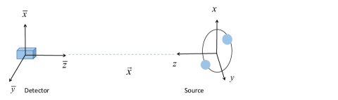
Figure 9: Sketch of THE propagation of GWs from a source to the detector. $(x,y,z)$ is the coordinate system of the source frame and $(\bar{x},\bar{y},\bar{z})$ is the coordinate system of observer’s frame.

References

- (1) B. P. Abbott et al. (LIGO Scientific Collaboration Virgo Collaboration), “GW150914: The Advanced LIGO Detectors in the Era of First Discoveries,” Phys. Rev. Lett. 116, no.13, 131103 (2016) [arXiv:1602.03838 [gr-qc]].
- (2) B. P. Abbott et al. (LIGO Scientific Collaboration Virgo Collaboration), “GW151226: Observation of Gravitational Waves from a 22-Solar-Mass Binary Black Hole Coalescence,” Phys. Rev. Lett. 116, no.24, 241103 (2016) [arXiv:1606.04855 [gr-qc]].
- (3) A. Einstein, Sitzungsberichte der Königlich Preussischen Akademie der Wissenschaften, Berlin, 1916; Sitzungsberichte der Königlich Preussischen Akademie der Wissenschaften, Berlin, 1918.
- (4) F. Ozel, D. Psaltis, R. Narayan and J. E. McClintock, “The Black Hole Mass Distribution in the Galaxy,” Astrophys. J. 725, 1918-1927 (2010) [arXiv:1006.2834 [astro-ph.GA]].
- (5) I. Mandel and S. E. de Mink, Mon. Not. Roy. Astron. Soc. 458, no.3, 2634-2647 (2016), [arXiv:1601.00007 [astro-ph.HE]]; P. Marchant, N. Langer, P. Podsiadlowski, T. M. Tauris and T. J. Moriya, Astron. Astrophys. 588, A50 (2016), [arXiv:1601.03718 [astro-ph.SR]]; S. de Mink and I. Mandel, Mon. Not. Roy. Astron. Soc. 460, no.4, 3545-3553 (2016), [arXiv:1603.02291 [astro-ph.HE]]; D. Kushnir, M. Zaldarriaga, J. A. Kollmeier and R. Waldman, Mon. Not. Roy. Astron. Soc. 462, no.1, 844-849 (2016), [arXiv:1605.03839 [astro-ph.HE]]; S. F. Portegies Zwart and S. McMillan, Astrophys. J. Lett. 528, L17 (2000), [arXiv:astro-ph/9910061 [astro-ph]]; C. L. Rodriguez, C. J. Haster, S. Chatterjee, V. Kalogera and F. A. Rasio, Astrophys. J. Lett. 824, no.1, L8 (2016), [arXiv:1604.04254 [astro-ph.HE]];
- (6) I. Dvorkin, E. Vangioni, J. Silk, J. P. Uzan and K. A. Olive, Mon. Not. Roy. Astron. Soc. 461, no.4, 3877-3885 (2016), [arXiv:1604.04288 [astro-ph.HE]]; C. L. Fryer, K. Belczynski, G. Wiktorowicz, M. Dominik, V. Kalogera and D. E. Holz, Astrophys. J. 749, 91 (2012), [arXiv:1110.1726 [astro-ph.SR]]; T. Kinugawa, K. Inayoshi, K. Hotokezaka, D. Nakauchi and T. Nakamura, Mon. Not. Roy. Astron. Soc. 442, no.4, 2963-2992 (2014), [arXiv:1402.6672 [astro-ph.HE]]; T. Kinugawa, A. Miyamoto, N. Kanda and T. Nakamura, Mon. Not. Roy. Astron. Soc. 456, no.1, 1093-1114 (2016), [arXiv:1505.06962 [astro-ph.SR]].
- (7) S. Bird, I. Cholis, J. B. Muoz, Y. Ali-Haïmoud, M. Kamionkowski, E. D. Kovetz, A. Raccanelli and A. G. Riess, Phys. Rev. Lett. 116, no.20, 201301 (2016), [arXiv:1603.00464 [astro-ph.CO]]; M. Sasaki, T. Suyama, T. Tanaka and S. Yokoyama, Phys. Rev. Lett. 117, no.6, 061101 (2016), [arXiv:1603.08338 [astro-ph.CO]]; K. Hayasaki, K. Takahashi, Y. Sendouda and S. Nagataki, Publ. Astron. Soc. Jap. 68, no.4, 66 (2016), [arXiv:0909.1738 [astro-ph.CO]].
- (8) T. Wang, L. Li, C. Zhu, Z. Wang, A. Wang, Q. Wu, H. S. Liu and G. Lü, Astrophys. J. 863, no.1, 17 (2018) [arXiv:1806.10266 [astro-ph.HE]].
- (9) B. P. Abbott et al. (LIGO Scientific Collaboration and Virgo Collaboration), “GW190814: Gravitational Waves from the Coalescence of a 23 Black Hole with a 2.6 Compact Object,” Astrophys. J. 896, no.2, L44 (2020), [arXiv:2006.12611[astro-ph.HE]]; and references therein.
- (10) B. P. Abbott et al. (LIGO Scientific Collaboration Virgo Collaboration), “GWTC-1: A Gravitational-Wave Transient Catalog of Compact Binary Mergers Observed by LIGO and Virgo during the First and Second Observing Runs,” Phys. Rev. X 9, no.3, 031040 (2019), [arXiv:1811.12907 [astro-ph.HE]].
- (11) R. Abbott et al. (LIGO Scientific Collaboration Virgo Collaboration), “Open data from the first and second observing runs of Advanced LIGO and Advanced Virgo,” [arXiv:1912.11716 [gr-qc]].
- (12) B. P. Abbott et al. (LIGO Scientific Collaboration Virgo Collaboration), “GW190425: Observation of a Compact Binary Coalescence with Total Mass ,” Astrophys. J. Lett. 892, L3 (2020), [arXiv:2001.01761 [astro-ph.HE]].
- (13) B. P. Abbott et al. (LIGO Scientific Collaboration Virgo Collaboration), “GW170104: Observation of a 50-Solar-Mass Binary Black Hole Coalescence at Redshift 0.2,” Phys. Rev. Lett. 118, no.22, 221101 (2017), [arXiv:1706.01812 [gr-qc]].
- (14) B. P. Abbott et al. (LIGO Scientific Collaboration Virgo Collaboration), “GW170608: Observation of a 19-solar-mass Binary Black Hole Coalescence,” Astrophys. J. 851, no.2, L35 (2017), [arXiv:1711.05578 [astro-ph.HE]].
- (15) B. P. Abbott et al. (LIGO Scientific Collaboration Virgo Collaboration), “GW170814: A Three-Detector Observation of Gravitational Waves from a Binary Black Hole Coalescence,” Phys. Rev. Lett. 119, no.14, 141101 (2017), [arXiv:1709.09660 [gr-qc]].
- (16) B. P. Abbott et al. (LIGO Scientific Collaboration Virgo Collaboration), “GW170817: Observation of Gravitational Waves from a Binary Neutron Star Inspiral,” Phys. Rev. Lett. 119, no.16, 161101 (2017), [arXiv:1710.05832 [gr-qc]].
- (17) https://www.ligo.caltech.edu/.
- (18) K. Somiya (KAGRA), “Detector configuration of KAGRA: The Japanese cryogenic gravitational-wave detector,” Class. Quant. Grav. 29, 124007 (2012), [arXiv:1111.7185 [gr-qc]].
- (19) M. Punturo et al.“The Einstein Telescope: A third-generation gravitational wave observatory,” Class. Quant. Grav. 27, 194002 (2010); S. Hild et al.“Sensitivity Studies for Third-Generation Gravitational Wave Observatories,” Class. Quant. Grav. 28, 094013 (2011), [arXiv:1012.0908 [gr-qc]].
- (20) B. P. Abbott et al. (LIGO Scientific Collaboration Virgo Collaboration), Class. Quant. Grav. 34, no.4, 044001 (2017), [arXiv:1607.08697 [astro-ph.IM]]; S. Dwyer, D. Sigg, S. W. Ballmer, L. Barsotti, N. Mavalvala and M. Evans, Phys. Rev. D 91, no.8, 082001 (2015), [arXiv:1410.0612 [astro-ph.IM]].
- (21) P. Amaro-Seoane et al. (LISA), “Laser Interferometer Space Antenna,” [arXiv:1702.00786 [astro-ph.IM]].
- (22) W. H. Ruan, C. Liu, Z. K. Guo, Y. L. Wu and R. G. Cai, “The LISA-Taiji network,” Nature Astron. 4, 108-109 (2020) [arXiv:2002.03603 [gr-qc]].
- (23) X. C. Hu, X. H. Li, Y. Wang, W. F. Feng, M. Y. Zhou, Y. M. Hu, S. C. Hu, J. W. Mei and C. G. Shao, “Fundamentals of the orbit and response for TianQin,” Class. Quant. Grav. 35, no.9, 095008 (2018) [arXiv:1803.03368 [gr-qc]].
- (24) S. Kawamura et al. “Current status of space gravitational wave antenna DECIGO and B-DECIGO,” [arXiv:2006.13545 [gr-qc]].
- (25) S. Vitale and M. Evans, “Parameter estimation for binary black holes with networks of third generation gravitational-wave detectors,” Phys. Rev. D 95, no.6, 064052 (2017), [arXiv:1610.06917 [gr-qc]].
- (26) N. Yunes, K. Yagi and F. Pretorius, “Theoretical Physics Implications of the Binary Black-Hole Mergers GW150914 and GW151226,” Phys. Rev. D 94, no.8, 084002 (2016), [arXiv:1603.08955 [gr-qc]].
- (27) C. M. Will, Living Rev. Rel. 17, 4 (2014), [arXiv:1403.7377 [gr-qc]]; N. Yunes and X. Siemens, Living Rev. Rel. 16, 9 (2013), [arXiv:1304.3473 [gr-qc]].
- (28) A. Ashtekar, B. Bonga and A. Kesavan, “Asymptotics with a positive cosmological constant: III. The quadrupole formula,” Phys. Rev. D 92, no.10, 104032 (2015), [arXiv:1510.05593 [gr-qc]].
- (29) Y. Z. Chu, “Transverse traceless gravitational waves in a spatially flat FLRW universe: Causal structure from dimensional reduction,” Phys. Rev. D 92, no.12, 124038 (2015), [arXiv:1504.06337 [gr-qc]].
- (30) L. Bieri, D. Garfinkle and S. T. Yau, “Gravitational wave memory in de Sitter spacetime,” Phys. Rev. D 94, no.6, 064040 (2016), [arXiv:1509.01296 [gr-qc]].
- (31) A. Kehagias and A. Riotto, “BMS in Cosmology,” JCAP 05, 059 (2016), [arXiv:1602.02653 [hep-th]].
- (32) A. Tolish and R. M. Wald, “Cosmological memory effect,” Phys. Rev. D 94, no.4, 044009 (2016), [arXiv:1606.04894 [gr-qc]].
- (33) A. Ashtekar and S. Bahrami, Phys. Rev. D 100, no.2, 024042 (2019) [arXiv:1904.02822 [gr-qc]]; P. K. Dunsby, B. A. Bassett and G. F. Ellis, Class. Quant. Grav. 14, 1215-1222 (1997), [arXiv:gr-qc/9811092 [gr-qc]]; M. Marklund, P. K. Dunsby and G. Brodin, Phys. Rev. D 62, 101501 (2000), [arXiv:gr-qc/0007035 [gr-qc]]; P. Hogan and E. O’Shea, Phys. Rev. D 65, 124017 (2002), [arXiv:gr-qc/0204050 [gr-qc]]; E. O’Shea, Phys. Rev. D 69, 064038 (2004), [arXiv:gr-qc/0401106 [gr-qc]].
- (34) R. d’Inverno, “Introducing Einstein’s relativity,” Revised Edition(Clarendon Press, Oxford, 1992).
- (35) Y. Z. Chu and G. D. Starkman, “Retarded Green’s Functions In Perturbed Spacetimes For Cosmology and Gravitational Physics,” Phys. Rev. D 84, 124020 (2011), [arXiv:1108.1825 [astro-ph.CO]].
- (36) J. Fier, X. Fang, B. Li, S. Mukohyama, A. Wang and T. Zhu, “Gravitational wave cosmology: High frequency approximation,” Phys. Rev. D 103, no.12, 123021 (2021), [arXiv:2102.08968 [astro-ph.CO]].
- (37) A. Wang, “Gravitational Faraday rotation induced from interacting gravitational plane waves,” Phys. Rev. D 44, 1120 (1991).
- (38) A. Wang, “Interacting Gravitational, Electromagnetic, Neutrino and Other Waves,” (World Scientific, 2020).
- (39) P. Szekeres, “Colliding plane gravitational waves,” J. Math. Phys. 13, 286-294 (1972).
- (40) J. Griffiths, “The Collision of Plane Waves in General Relativity,” Annals Phys. 102, 388-404 (1976).
- (41) J. B. Griffiths, “Colliding plane waves in general relativity,” (Dpver Publications, Inc. Mineola, New York, 2016).
- (42) S. Hou, X. L. Fan and Z. H. Zhu, “Gravitational Lensing of Gravitational Waves: Rotation of Polarization Plane,” Phys. Rev. D 100, no.6, 064028 (2019), [arXiv:1907.07486 [gr-qc]].
- (43) E. Newman and R. Penrose, “An Approach to gravitational radiation by a method of spin coefficients,” J. Math. Phys. 3, 566-578 (1962).
- (44) P. Szekeres, “The Gravitational compass,” J. Math. Phys. 6, 1387-1391 (1965).
- (45) S. Hawking and G. Ellis, “The Large Scale Structure of Space-Time” (Cambridge University Press, Cambridge, 1973).
- (46) B. Ryden, “Introduction to cosmology” (Addison Wesley, New York, 2003).
- (47) N. Aghanim et al. [Planck Collaboration], “Planck 2018 results. VI. Cosmological parameters,” [arXiv:1807.06209 [astro-ph.CO]].
- (48) R. K. Sachs, “Gravitational radiation,” in Relativité, Groupes et Topologie, Les Houches Summer Shcool of Theoretical Physics, C. DeWitt and B.S. DeWitt (Eds.) (Gordon and Breach Science Publishers, New York, 1964).
- (49) J. M. Stewart and M. Walker, “Perturbations of spacetimes in general relativity,” Proc. Roy. Soc. Lond. A 341, 49-74 (1974).
- (50) A. S. Miranda, J. Morgan, V. T. Zanchin and A. Kandus, “Separable wave equations for gravitoelectromagnetic perturbations of rotating charged black strings,” Class. Quant. Grav. 32, no.23, 235002 (2015), [arXiv:1412.6312 [gr-qc]].
- (51) M. Maggiore, “Gravitational Waves. Vol. 1: Theory and Experiments,” (Oxford University Press, Oxford, 2016).
- (52) M. Maggiore, “Gravitational waves and fundamental physics,” [arXiv:gr-qc/0602057 [gr-qc]].
- (53) S. Hou, X. L. Fan and Z. H. Zhu, “Corrections to the gravitational wave phasing,” Phys. Rev. D 101, 084052 (2020), [arXiv:1911.04182 [gr-qc]].