Joint Analysis of Sound Events and Acoustic Scenes
Using Multitask Learning

Abstract

Sound event detection (SED) and acoustic scene classification (ASC) are important research topics in environmental sound analysis. Many research groups have addressed SED and ASC using neural-network-based methods, such as the convolutional neural network (CNN), recurrent neural network (RNN), and convolutional recurrent neural network (CRNN). The conventional methods address SED and ASC separately even though sound events and acoustic scenes are closely related to each other. For example, in the acoustic scene “office,” the sound events “mouse clicking” and “keyboard typing” are likely to occur. Therefore, it is expected that information on sound events and acoustic scenes will be of mutual aid for SED and ASC. In this paper, we propose multitask learning for joint analysis of sound events and acoustic scenes, in which the parts of the networks holding information on sound events and acoustic scenes in common are shared. Experimental results obtained using the TUT Sound Events 2016/2017 and TUT Acoustic Scenes 2016 datasets indicate that the proposed method improves the performance of SED and ASC by 1.31 and 1.80 percentage points in terms of the F-score, respectively, compared with the conventional CRNN-based method.

Index Terms—  Sound event detection, acoustic scene classification, multitask learning, convolutional recurrent neural network

1 Introduction

There has been renewed interest in the automatic analysis of various environmental sounds in our everyday lives [1]. The ability to automatically analyze environmental sounds will give rise to various applications, such as anomalous sound detection systems [2], automatic life-logging systems [3, 4], monitoring systems [5, 6], and hearing-impaired support systems [7, 8]. In environmental sound analysis, two tasks have primarily been studied: sound event detection (SED) and acoustic scene classification (ASC). SED is the identification of sound event labels and detection of their boundaries in audio signals, where a sound event represents a type of sound such as “car horn,” “people walking,” or “keyboard typing.” On the other hand, ASC is the identification of acoustic scene labels from a recorded sound, where an acoustic scene represents a recording location, situation, or human activity such as “city center,” “on the bus,” or “cooking.” For SED and ASC, various methods using the Gaussian mixture model (GMM) [9, 10], hidden Markov model (HMM) [11, 12], and support vector machine (SVM) [13], have been proposed. In SED, since multiple sound events often occur simultaneously, polyphonic SED methods, which can detect multiple overlapping sound events, have been proposed. Some works have applied non-negative matrix factorization (NMF) [14, 15] for polyphonic SED, wherein the spectrogram of input sound is decomposed into a product of a basis and activation matrix. Each basis and activation vector represent a single sound event and the active duration of the corresponding event, respectively. More recently, in sound event and acoustic scene analysis there has been a growing trend towards the use of deep neural networks (DNNs) [16, 17], which outperform the conventional methods based on the GMM, HMM, and SVM.

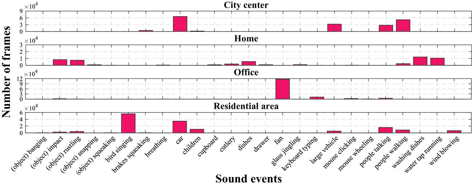
Fig. 1: Number of frames of sound events for each acoustic scene in dataset used for our evaluation experiments.

None of the studies on SED and ASC have tackled sound event and acoustic scene analysis jointly; however, in many cases, sound events and acoustic scenes are associated with each other. For instance, in the acoustic scene “office,” the sound events “mouse clicking” and “keyboard typing” are likely to occur, whereas the sound events “car” and “bird singing” rarely occur. That is, when analyzing the sound events “mouse clicking” and “keyboard typing,” it is expected that information on the acoustic scene “office” will help recognize these sound events. Similarly, information on the sound events “mouse clicking,” and “keyboard typing” can help to predict the acoustic scene “office.” On the basis of this concept, SED taking information on acoustic scenes into account [18, 19, 20] and ASC utilizing information on sound events [21] have been proposed. However, these conventional methods do not analyze both sound events and scenes simultaneously. Moreover, these methods cannot be applied to state-of-the-art neural-network-based methods.

To address this problem, we have proposed a method for joint analysis of sound events and acoustic scenes using multitask learning [22]. Multitask learning is a method for learning related multiple tasks simultaneously by sharing the parameters of machine learning models [23]. In speech processing, it has been reported that multitask learning improves the performance of speech recognition [24, 25]. In the analysis of environmental sounds, ASC using environment-based scene grouping and multitask learning of multiple classification networks of grouped scenes (e.g., indoor/outdoor scene) [26], and SED with the multitask learning of event detection and timestamp identification [27, 28], have been proposed. In this paper, we discuss the method for joint analysis of sound events and acoustic scenes using multitask learning in detail, and we investigate the performance of the proposed multitask-learning-based method in detail. The contribution of the proposed method is as follows.

• We discuss in detail a new method for joint analysis of sound events and acoustic scenes utilizing multitask learning combining SED and ASC methods.

• We demonstrate that the multitask-learning-based method improves SED and ASC performances.

The rest of this paper is organized as follows. In Section 2, we discuss conventional methods for SED and ASC and the proposed method for the joint analysis of sound events and scenes utilizing multitask learning. In Section 3, we report the results of experiments conducted to evaluate the performance of event detection and scene classification. We then conclude this paper in Section 4.

2 Conventional Methods for SED and ASC

In this section, we overview conventional SED and ASC methods using neural networks.

SED involves the estimation of sound event categories and their time boundaries. In recent years, a number of neural-network-based approaches, such as those using the convolutional neural network (CNN) [29], recurrent neural network (RNN) [30], and convolutional recurrent neural network [31, 32], have been proposed. Specifically, it has been reported that methods in which the CNN and bidirectional gated recurrent unit (BiGRU) are combined detect sound events with reasonable performance [31, 32]. In the CNN–BiGRU-based method, the acoustic feature ${\bf X}\in\mathbb{R}^{D\times T}$, which is a time–frequency representation of the acoustic signal, is input to the network. Here, $D$ and $T$ are the numbers of frequency bins and time frames of the input feature map, respectively. The convolutional layer convolutes the input feature map with two-dimensional filters, and max pooling is then performed to reduce the dimension $D$ of the feature map. The output of the convolutional layer ${\bf c}_{t}^{(d^{\prime},c)}$ in time frame $t$ $\in\mathbb{R}^{D^{\prime}\times C}$ is then concatenated as ${\bf c^{\prime}}=({\bf c}_{t}^{(1,1)},{\bf c}_{t}^{(1,2)},\ldots,{\bf c}_{t}^{(1,C)},{\bf c}_{t}^{(2,1)},\ldots,{\bf c}_{t}^{(D^{\prime},C)}$), and then ${\bf c^{\prime}}$ is fed to layers of the BiGRU, where $C$ is the number of convolution filters. After that, the output vector ${\bf h}_{t}$ is calculated using the following set of equations:

$${\bf g}^{f}_{t} =\sigma({\bf W}^{f}_{g}{\bf c}^{\prime}_{t}+{\bf U}^{f}_{g}{\bf h}_{t-1}+{\bf b}^{f}_{g}),$$ (1)

$${\bf r}^{f}_{t} =\sigma({\bf W}^{f}_{r}{\bf c}^{\prime}_{t}+{\bf U}^{f}_{r}{\bf h}_{t-1}+{\bf b}^{f}_{r}),$$ (2)

$${\bf h}^{f}_{t} =(1-{\bf g}^{f}_{t})\odot{\bf h}_{t-1}$$

$$\hskip 10.0pt+{\bf g}^{f}_{t}\odot\tanh({\bf W}^{f}_{h}{\bf c}^{\prime}_{t}+{\bf U}^{f}_{h}({\bf r}^{f}_{h}{\bf h}_{t-1})+{\bf b}^{f}_{h}),$$ (3)

$${\bf g}^{b}_{t} =\sigma({\bf W}^{b}_{g}{\bf c}^{\prime}_{t}+{\bf U}^{b}_{g}{\bf h}_{t+1}+{\bf b}^{b}_{g}),$$ (4)

$${\bf r}^{b}_{t} =\sigma({\bf W}^{b}_{r}{\bf c}^{\prime}_{t}+{\bf U}^{b}_{r}{\bf h}_{t+1}+{\bf b}^{b}_{r}),$$ (5)

$${\bf h}^{b}_{t} =(1-{\bf g}^{b}_{t})\odot{\bf h}_{t+1}$$

$$\hskip 10.0pt+{\bf g}^{b}_{t}\odot\tanh({\bf W}^{b}_{h}{\bf c}^{\prime}_{t}+{\bf U}^{b}_{h}({\bf r}^{b}_{h}{\bf h}_{t+1})+{\bf b}^{b}_{h}),$$ (6)

$${\bf h}_{t} =\begin{bmatrix}{\bf h}^{f}_{t}\\[3.0pt] {\bf h}^{b}_{t}\end{bmatrix},$$ (7)

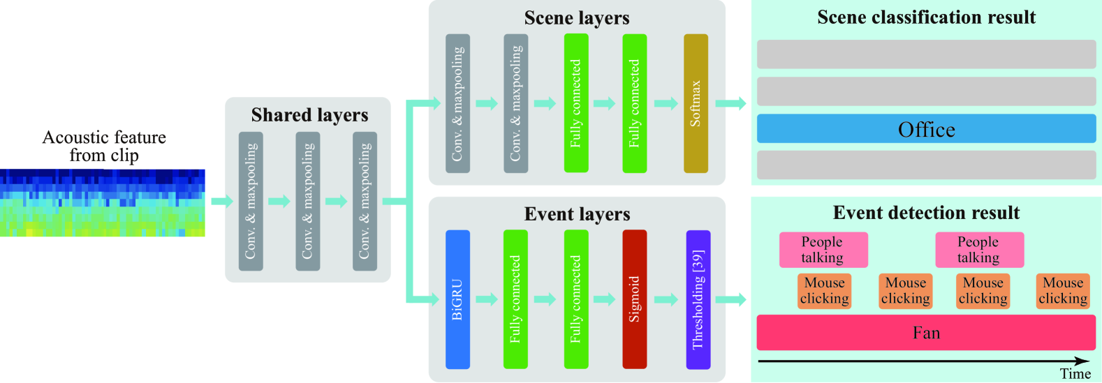
Fig. 2: Example of network structure for proposed multitask learning of sound events and acoustic scenes. In shared layers, information on sound events and scenes in common is extracted. In event and scene layers, event- and scene-specific features are extracted, respectively.

where ${\bf W}$ and ${\bf U}$ are parameter matrices and ${\bf b}$ is a bias vector. Subscripts $g$ and $r$ indicate the update gate and reset gate, respectively. Superscripts $f$ and $b$ are the forward and backward networks, respectively. ${\bf g}$, ${\bf r}$, $\odot$, and $\sigma$ indicate the update gate vector, reset gate vector, Hadamard product, and sigmoid function, respectively. The BiGRU layer is followed by a fully connected (FC) layer, and the output layer of the network is finally calculated as

$${\bf y}_{t}=\sigma({\bf h}_{t}).$$ (8)

The network parameters of the CNN–BiGRU method are optimized with the following sigmoid cross-entropy objective function ${\mathcal{L}}_{\rm event}({\bm{\Theta}}_{1})$ using backpropagation through time (BPTT):

$$\ {\mathcal{L}}_{\rm event}({\bm{\Theta}}_{1}) =-\!\sum^{T}_{t=1}{\big{\{}}{\bf z}_{t}\log({\bf y}_{t})+(1-{\bf z}_{t})\log(1-{\bf y}_{t}){\big{\}}}$$

$$=-\!\sum^{M}_{m=1}\sum^{T}_{t=1}\!{\Big{\{}}z_{m,t}\log y_{m,t}\!+\!(1\!-\!z_{m,t})\log{\big{(}}1\!-\!y_{m,t}{\big{)}}{\Big{\}}},$$ (9)

where ${\bm{\Theta}}_{1}$, $M$, and $m$ are the network parameters of the CNN–BiGRU method, the number of sound event categories, and the index of the event category, respectively. $z_{m,t}$ is the target label in time frame $t$, which is 1 if sound event $m$ is active in time frame $t$, and 0 otherwise.

ASC involves the classification of an audio recording into one of the predefined classes of the acoustic scene. Several lines of evidence indicate that CNN-based approaches achieve state-of-the-art performance in ASC [33, 34]. In CNN-based ASC, the time–frequency representation of acoustic signal ${\bf X}$ is fed to a two-dimensional convolutional layer, where the input feature map is also compressed, as with the CNN layer in SED. The output of the CNN layer is then concatenated and input to a fully connected layer, and the output layer of the network is finally calculated as

$${\bf y}_{t} =S({\bf h}_{t}),$$ (10)

where $S$ denotes the softmax function. The network is optimized under the following softmax cross-entropy objective function ${\mathcal{L}}_{\rm scene}({\bm{\Theta}}_{2})$:

$${\mathcal{L}}_{\rm scene}({\bm{\Theta}}_{2})=-\sum^{N}_{n=1}{\Big{\{}}z_{n}\log S(y_{n}){\Big{\}}},$$ (11)

where ${\bm{\Theta}}_{2}$ is the parameter of the network for ASC. $N$, $n$, and $z_{n}$ are the number of the acoustic scene categories, the index of the scene categories, and the target scene label, respectively.

3 Joint Analysis of Sound Events and Scenes Based on Multitask Learning

In conventional works addressing SED and ASC, they have been studied separately. However, many sound events and acoustic scenes are related to each other. Fig. 1 shows the number of time frames of the sound events for each acoustic scene in a development dataset used for experiments. This figure indicates that the occurrence of sound events is biased for acoustic scenes; thus, sound events and acoustic scenes are key information in their mutual identification. On the basis of this idea, we have proposed the multitask learning of sound events and acoustic scenes, in which the parts of the networks holding information on sound events and scenes in common are shared. Multitask learning to jointly analyze multiple tasks has been proposed by Caruana [23], and it has been reported that when multiple tasks are related to each other, it achieves better performance than a single-task method.

The concept of the proposed method is illustrated in Fig. 2. We refer to the shared part of the network as the “shared layers,” and the following scene-specific layers and event-specific layers as the “scene layers” and “event layers,” respectively. The “shared layers” are expected to capture the information common to sound events and scenes from audio clips. The features are fed into each specific layer to tune each model of SED/ASC. The “event” and “scene layers” extract event- and scene-specific features, respectively. After that, each output of specific layers is utilized for scene classification or event detection. In this work, we apply the CRNN as the event detection network and the CNN as the scene classification network, and the layers of the CNN are shared between the event detection and scene classification networks.

To optimize this network, the following objective function is applied:

$${\mathcal{L}}({\bm{\Theta}})=\alpha{\mathcal{L}}_{\rm event}({\bm{\Theta}}_{1})+\beta{\mathcal{L}}_{\rm scene}({\bm{\Theta}}_{2}),$$ (12)

where ${\bm{\Theta}}$ denotes the parameters of the proposed network. $\alpha$ and $\beta$ are the weights of the objective functions for SED and ASC, respectively. In this work, we set $\alpha$ as 1.0 because $\alpha$ can be set as 1.0 without loss of generality in many of optimization algorithms such as stochastic gradient descent (SGD) and Adam. Note that the proposed method can also be applied to any network that can be optimized by Eq. (12).

4 Experiments

4.1 Experimental Conditions

To evaluate the performances of SED and ASC using the proposed multitask method, we conducted evaluation experiments using the TUT Sound Events 2016 [35], TUT Sound Events 2017 [33], TUT Acoustic Scenes 2016 [35], and TUT Acoustic Scenes 2017 [33] datasets. From these datasets, we selected sound clips including four acoustic scenes, “home,” “residential area” (TUT Sound Events 2016), “city center” (TUT Sound Events 2017, TUT Acoustic Scenes 2017), and “office” (TUT Acoustic Scenes 2016), which contain 266 min (development set: 192 min, evaluation set: 74 min) of audio. Here, the acoustic scene “office” in TUT Acoustic Scenes 2016 and “city center” in TUT Acoustic Scenes 2017 did not have sound event labels; thus, we manually annotated the sound clips with sound event labels by the procedure described in [35, 33]. These sound clips include the 25 types of sound event labels listed in Fig. 1. The sound event labels annotated for this experiment are available in [36].

As acoustic features, we used 64-dimensional log-mel energies calculated for each 40 ms time frame with 50% overlap. This setting is based on the baseline system of DCASE2018 Challenge task4 [37] and a work that won the first place in DCASE2019 Challenge task4 [38]. The acoustic features were then input to the network shown in Fig. 2. The model parameter was tuned using only the development dataset. We then evaluated the performance of our proposed model using evaluation dataset. Active sound events were predicted using adaptive thresholds [39] tuned for each sound event using the development dataset. Each model was trained and evaluated ten times with various initial values of model parameters. Other experimental conditions are listed in Table 1.

As comparative methods, we also evaluated the detection performance for sound events by CNN method (referred to as CNN (event)) and the CNN–BiGRU method (referred to as CRNN (event)), and the classification performance for acoustic scenes by the CNN method (referred to as CNN (scene)). CRNN (event) and CNN (event) have the same structures as the shared + event and shared layers in Fig. 2, respectively. CNN (scene) has the same structure as the shared and scene layers in the proposed method. Moreover, to verify the utility of the proposed method, we compared the proposed method with a SED method based on multitask learning of SED and sound activity detection [27] (referred to as SED + SAD), and the proposed method + the conventional method using SAD [27] (referred to as proposed + SAD).

Table 1: Experimental conditions

Acoustic feature	Log-mel energy (64 dim.)
Frame length / shift	40 ms / 20 ms
Length of sound clip	10 s
Shared layer
Network of shared layers	3 CNN
# channels of CNN layers	128, 128, 128
Filter size	3$\times$3
Pooling size	8$\times$1, 2$\times$1, 2$\times$1 (max pooling)
Scene layer
Network of scene layers	2 CNN & 1 FC layers
# channels of CNN layers	256, 256
Filter size	3$\times$3
Pooling size	1$\times$25, 1$\times$20 (max pooling)
# units in FC layer	32
Event layer
Network of event layers	1 BiGRU & 1 FC layers
# units in GRU layer	32
# units in FC layer	32

4.2 Metrics

In SED, since sound events may overlap, the event detection performance was evaluated on the basis of a segment-based F-score and error rate (ER) [40]. To calculate the segment-based F-score, the precision and recall were first calculated as

$${\rm Precision} =\frac{{\rm TP}}{{\rm TP}+{\rm FP}},$$ (13)

$${\rm Recall} =\frac{{\rm TP}}{{\rm TP}+{\rm FN}},$$ (14)

where TP, FP, and FN are the total counts of true positive, false positive, and false negative for all time frames and sound events, respectively. The segment-based F-score was then calculated as

$${\rm F\textrm{-}score}=\frac{2\cdot{\rm Precision}\cdot{\rm Recall}}{{\rm Precision}+{\rm Recall}}.$$ (15)

To calculate the segment-based ER, we first calculated substitutions (S), deletions (D), and insertions (I) as

$${\rm S}(k) =\min({\rm FN}(k),{\rm FP}(k)),$$ (16)

$${\rm D}(k) =\max(0,{\rm FN}(k)-{\rm FP}(k)),$$ (17)

$${\rm I}(k) =\max(0,{\rm FP}(k)-{\rm FN}(k)),$$ (18)

where $k$ indicates the index of the time frame. We then calculated the ER as

$${\rm ER}=\frac{\sum_{k=1}^{K}{\rm S}(k)+\sum_{k=1}^{K}{\rm D}(k)+\sum_{k=1}^{K}{\rm I}(k)}{\sum_{k=1}^{K}{\rm N}(k)},$$ (19)

where $K$ and $N(k)$ are the total number of time frames and the number of sound events in time frame $k$, respectively.

On the other hand, ASC is a simple classification task and acoustic scenes do not overlap in time. We thus calculated the F-score using Eqs. (13) – (15), where TP, FP, and FN are the total numbers of sound clips of true positive, false positive, and false negative, respectively.

Table 2: Performances of sound event detection and scene classification

Method	Event		Scene
	F-score	ER	F-score
CNN (event)	34.67%	1.310	-
CRNN (event)	44.88%	1.301	-
CNN (scene)	-	-	67.35%
SED + SAD [27]	47.59%	1.081	-
Proposed ($\beta$=10.0)	21.85%	4.531	69.15%
Proposed ($\beta$=0.01)	45.76%	1.119	65.17%
Proposed ($\beta$=0.0001)	46.19%	1.102	61.89%
Proposed + SAD ($\beta=0.01$)	48.99%	0.908	60.02%

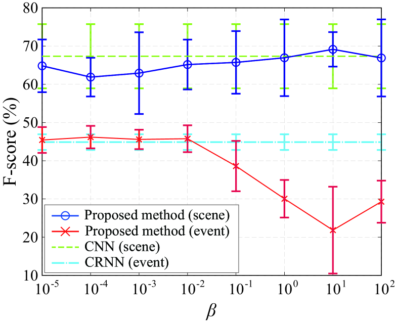
Fig. 3: Sound event detection and scene classification performance as functions of weight $\beta$

Table 3: Sound event detection performance for each event

Event		(object)	(object)	(object)	(object)	(object)	bird	brakes	breathing	car	children	cupboard	cutlery
		banging	impact	rustling	snapping	squeaking	singing	squeaking
CRNN	F-score	0.00%	9.56%	13.89%	0.00%	0.00%	47.01%	7.73%	0.00%	51.75%	6.10%	0.00%	0.39%
(event)
	ER	1.007	1.346	3.542	1.002	1.000	1.538	1.022	1.008	1.740	1.491	1.000	1.018
Proposed	F-score	0.00%	8.82%	13.30%	0.00%	0.00%	48.88%	6.61%	0.00%	50.97%	3.54%	0.00%	0.11%
($\beta$=0.0001)
	ER	1.122	1.252	3.393	1.004	1.000	1.448	0.975	1.012	1.686	1.334	1.000	1.004

Event		​dishes​	​drawer​	​fan​	​glass​	​keyboard​	​large​	​mouse​	​mouse​	​people​	​people​	​washing​	​water tap​	​wind​
					​jingling​	​typing​	​vehicle​	​clicking​	​wheeling​	​talking​	​walking​	​dishes​	​running​	​blowing​
CRNN	F-score	11.29%	0.00%	71.97%	0.00%	4.29%	17.55%	0.02%	0.00%	2.48%	15.34%	38.44%	66.32%	15.96%
(event)
	ER	1.076	1.000	0.733	1.011	1.805	4.642	1.025	1.003	3.391	1.559	2.029	0.659	1.036
Proposed	F-score	6.94%	0.00%	72.31%	0.00%	5.00%	20.12%	0.30%	0.00%	2.75%	15.04%	35.54%	60.80%	8.81%
($\beta$=0.0001)
	ER	1.041	1.000	0.633	1.005	1.389	2.634	1.007	1.001	2.725	1.396	1.845	0.707	0.997

4.3 Experimental Results

4.3.1 Overall Performances of SED and ASC

Table 2 shows the experimental results of using the conventional methods and the proposed multitask-based method. The results show that the proposed multitask-based method enables the joint analysis of sound events and acoustic scenes with a reasonable performance compared with CRNN (event) and CNN (scene). Moreover, when $\beta$ = 0.0001 (Proposed), the F-score of event detection by the proposed method was improved by 1.31 points compared with that of the conventional CRNN (event). When $\beta$ = 10.0 (Proposed), the F-score of scene classification of the proposed method was improved by 1.80 percentage points compared with that of the conventional CNN (scene). These results indicate that information on sound events and acoustic scenes are mutually helpful in SED method and ASC.

To further demonstrate the utility of the proposed method, we applied our method to the conventional method for SED [27], which is based on the multitask learning of SED and SAD. The experimental results show that the event detection performance of SED + SAD [27] is better than that of CRNN (event). Moreover, the F-score of event detection in proposed + SAD ($\beta$= 0.01) was improved by 1.4 percentage points compared with that of SED + SAD [27]. The results indicate that the proposed method improves the SED performance when using not only CNN–BiGRU but also other models.

Further experiments were conducted to examine how the proposed method performs with various $\beta$. Fig. 3 shows the performances of event detection and scene classification for various $\beta$. The results show that when $\beta$ is less than or equal to 0.01, the SED performance of the proposed method is better than that of CRNN (event). When $\beta$ is larger than 1, the proposed method achieves a better ASC performance than CNN (scene), whereas the detection performance of sound events by the proposed method was worse than that by the conventional CRNN (event). When $\beta$ takes a large or small value, the ASC and SED performances of the proposed method agree well with those of the conventional CNN (scene) and CRNN (event), respectively. This is because when $\beta$ is small, the proposed method approximately works as CRNN (event), whereas when $\beta$ is large, the proposed method tends to ignore the sound event loss ${\bm{\Theta}}_{1}$.

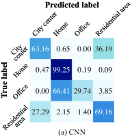
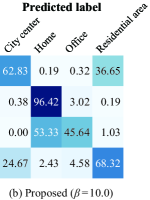
Fig. 4: Performance of acoustic scene classification for each scene in terms of recall (%)

Table 4: Performance of SED for each event and scene in terms of false-positive rate (FPR)

Event		(object)	(object)	(object)	(object)	(object)	bird	brakes	breathing	car	children	cupboard	cutlery
		banging	impact	rustling	snapping	squeaking	singing	squeaking
City	CRNN	0.0000	0.0070	0.0001	0.0000	0.0000	0.1150	0.0004	0.0000	0.5835	0.0043	0.0000	0.0000
center
	Proposed	0.0002	0.0014	0.0000	0.0000	0.0000	0.1073	0.0001	0.0000	0.5457	0.0038	0.0000	0.0000
Home	CRNN	0.0000	0.0409	0.1175	0.0000	0.0000	0.0146	0.0002	0.0000	0.0263	0.0041	0.0000	0.0004
	Proposed	0.0000	0.0352	0.1110	0.0000	0.0000	0.0115	0.0000	0.0001	0.0367	0.0010	0.0000	0.0001
Office	CRNN	0.0000	0.0011	0.0041	0.0000	0.0000	0.0062	0.0000	0.0000	0.0000	0.0002	0.0000	0.0000
	Proposed	0.0000	0.0036	0.0073	0.0000	0.0000	0.0028	0.0000	0.0000	0.0000	0.0003	0.0000	0.0000
Residential	CRNN	0.0000	0.0026	0.0094	0.0000	0.0000	0.3011	0.0038	0.0000	0.1837	0.0049	0.0000	0.0000
area
	Proposed	0.0000	0.0008	0.0056	0.0000	0.0000	0.2696	0.0005	0.0000	0.1684	0.0036	0.0000	0.0000

Event		​dishes​	​drawer​	​fan​	​glass​	​keyboard​	​large​	​mouse​	​mouse​	​people​	​people​	​washing​	​water tap​	​wind
					​jingling​	​typing​	​vehicle​	​clicking​	​wheeling​	​talking​	​walking​	​dishes​	​running​	​blowing
City	CRNN	0.0007	0.0000	0.0024	0.0000	0.0007	0.3268	0.0000	0.0000	0.0521	0.0656	0.0000	0.0009	0.0000
center
	Proposed	0.0007	0.0000	0.0041	0.0000	0.0000	0.1552	0.0000	0.0000	0.0342	0.0434	0.0000	0.0004	0.0002
Home	CRNN	0.0085	0.0000	0.4151	0.0001	0.0304	0.0002	0.0004	0.0000	0.0242	0.0008	0.2034	0.0815	0.0010
	Proposed	0.0042	0.0000	0.2816	0.0000	0.0147	0.0000	0.0001	0.0000	0.0075	0.0003	0.1663	0.0680	0.0005
Office	CRNN	0.0000	0.0000	0.0011	0.0000	0.0052	0.0000	0.0000	0.0000	0.0061	0.0001	0.0023	0.0000	0.0000
	Proposed	0.0000	0.0000	0.0008	0.0000	0.0039	0.0000	0.0000	0.0000	0.0020	0.0001	0.0009	0.0000	0.0000
Residential	CRNN	0.0000	0.0000	0.0531	0.0000	0.0003	0.0099	0.0000	0.0000	0.1124	0.0697	0.0000	0.0009	0.0041
area
	Proposed	0.0000	0.0000	0.0480	0.0000	0.0002	0.0029	0.0000	0.0000	0.0983	0.0589	0.0000	0.0001	0.0010

4.3.2 Detailed Investigation of ASC Performance

Fig. 4 shows confusion matrices of the scene classification performances in terms of recall. The left and right confusion matrices depict the performances of the conventional CNN (scene) and the proposed multitask-based method ($\beta$=10.0), respectively. The results indicate that the proposed method achieves better classification performance than the conventional CNN (scene). In particular, the recall for the acoustic scene “office” increases by 15.90 percentage points compared with that of the conventional CNN (scene). This is because the acoustic scene “office” has the dominant sound event “fan,” which occurs only in the acoustic scene “office,” and thus, information on the sound event “fan” significantly contributes to the classification of the acoustic scene “office.” On the other hand, little improvement of the scene classification performance for the acoustic scenes “city center” and “residential area” was observed. In the acoustic scenes “city center” and “residential area,” common sound events “car,” “children,” and “large vehicle” occur; thus, information of sound events may make a smaller contribution to the classification of these acoustic scenes.

4.3.3 Sound Event Detection Performance for Each Sound Event and Scene

We list the detection results of sound events for each event in Table 3. In this experiment, we evaluated the detection performance using $\beta=0.0001$. The proposed method achieves a better ER than the conventional CRNN (event) in most of the sound events. These results show that the proposed method reduces the misdetection of sound events. Moreover, the sound events “fan,” “keyboard typing,” and “mouse clicking” can be detected more accurately by the proposed method. As shown in Fig. 1, this is because these events are closely related to the particular acoustic scene “office,” and such information on the acoustic scene is helpful in detecting the sound events.

To investigate how the misdetection of sound events is reduced in the proposed method, we show the misdetection rate of the sound events for each event and scene in Table 4. In this experiment, we evaluated the detection performance using $\beta=0.0001$. To evaluate the rate of misdetection of sound events for each event and scene, we define the false-positive rate (FPR) because Eq. (19) cannot be calculated when $\sum_{k=1}^{K}{\rm N}(k)$ equals 0. Then the FPR is calculated as

$${\rm FPR}=\frac{\sum_{k=1}^{K}{\rm FP}(k)}{{\it K}}.$$ (20)

The results show that the proposed multitask-based method achieves a much better FPR in most of the sound events than the conventional CRNN-based method. In particular, the misdetection rate of the sound events “bird singing” and “fan,” which are closely related to the scenes “residential area” and “city,” respectively, can be significantly decreased by using the multitask-based method.

4.3.4 Calculation cost of models

To verify the calculation cost of our method, we compared the numbers of parameters of CRNN (event), CNN (scene), and the multitask-based model. Table 5 shows the number of parameters of each model. The results indicate that the multitask-based model has more parameters compared with CRNN (event). On the other hand, CNN (scene) has a comparable number of parameters to the multitask-based model. This is because scene-specific layers are mainly composed of CNN structures with many channels.

Table 5: Numbers of model parameters

Method	# of parameters
CRNN (event)		355,801
CNN (scene)		1,200,036
Proposed		1,258,621

5 Conclusion

In this paper, we discussed in detail a proposed method for joint analysis of sound events and acoustic scenes using multitask learning. In the proposed method, we applied a CRNN for SED and a CNN for ASC, and the CNN layers in both networks were shared in order to hold information on sound events and scenes in common. We integrated the objective functions of the event detection network and scene classification network using a weight parameter and optimized the network. Experimental results indicated that the proposed method enables joint analysis of sound events and scenes with reasonable performance compared with the conventional CRNN- and CNN-based methods. Moreover, the F-scores of the proposed method for SED and ASC are improved by 1.31 and 1.80 percentage point, respectively, compared with those of the conventional methods.

6 Acknowledgement

This work was supported by JSPS KAKENHI Grant Number JP19K20304 and the NVIDIA GPU Grant Program.

References

- [1] K. Imoto, “Introduction to acoustic event and scene analysis,” Acoust. Sci. Tech., vol.39, no.3, pp.182–188, 2018.
- [2] C. Chan and E. W. M. Yu, “An abnormal sound detection and classification system for surveillance applications,” Proc. European Signal Processing Conference (EUSIPCO), pp.1851–1855, 2010.
- [3] J. A. Stork, L. Spinello, J. Silva, and K. O. Arras, “Audio-based human activity recognition using non-Markovian ensemble voting,” Proc. IEEE International Symposium on Robot and Human Interactive Communication (RO-MAN), pp.509–514, 2012.
- [4] K. Imoto, S. Shimauchi, H. Uematsu, and H. Ohmuro, “User activity estimation method based on probabilistic generative model of acoustic event sequence with user activity and its subordinate categories,” Proc. INTERSPEECH, pp.2609–2613, 2013.
- [5] A. Harma, M. F. McKinney, and J. Skowronek, “Automatic surveillance of the acoustic activity in our living environment,” Proc. IEEE International Conference on Multimedia and Expo (ICME), pp.634–637, 2005.
- [6] S. Ntalampiras, I. Potamitis, and N. Fakotakis, “On acoustic surveillance of hazardous situations,” Proc. IEEE International Conference on Acoustics, Speech and Signal Processing (ICASSP), pp.165–168, 2009.
- [7] Y. T. Peng, C. Y. Lin, M. T. Sun, and K. C. Tsai, “Healthcare audio event classification using hidden Markov models and hierarchical hidden Markov models,” Proc. IEEE International Conference on Multimedia and Expo (ICME), pp.1218–1221, 2009.
- [8] P. Guyot, J. Pinquier, and R. André-Obrecht, “Water sound recognition based on physical models,” Proc. IEEE International Conference on Acoustics, Speech and Signal Processing (ICASSP), pp.793–797, 2013.
- [9] Z. Xiaodan, J. Huang, G. Potamianos, and M. Hasegawa-Johnson, “Acoustic fall detection using Gaussian mixture models and GMM supervectors,” Proc. IEEE International Conference on Acoustics, Speech and Signal Processing (ICASSP), pp.69–72, 2009.
- [10] S. Yun, S. Kim, S. Moon, J. Cho, and T. Kim, “Discriminative training of GMM parameters for audio scene classification,” Tech. Rep. DCASE 2016 Challenge, 2016.
- [11] A. Mesaros, T. Heittola, A. Eronen, and T. Virtanen, “Acoustic event detection in real life recordings,” Proc. European Signal Processing Conference (EUSIPCO), pp.1267–1271, 2010.
- [12] A. J. Eronen, V. T. Peltonen, J. T. Tuomi, A. P. Klapuri, S. Fagerlund, T. Sorsa, G. Lorho, and J. Huopaniemi, “Audio-based context recognition,” IEEE Trans. Audio Speech Lang. Process., vol.14, no.1, pp.321–329, 2006.
- [13] A. Rakotomamonjy and G. Gasso, “Histogram of gradients of time-frequency representations for audio scene classification,” IEEE/ACM Trans. Audio Speech Lang. Process., vol.23, no.1, pp.142–153, 2015.
- [14] J. F. Gemmeke, L. Vuegen, P. Karsmakers, B. Vanrumste, and H. Van hamme, “An exemplar-based NMF approach to audio event detection,” Proc. IEEE Workshop on Applications of Signal Processing to Audio and Acoustics (WASPAA), pp.1–4, 2013.
- [15] T. Komatsu, T. Toizumi, R. Kondo, and Y. Senda, “Acoustic event detection method using semi-supervised non-negative matrix factorization with mixtures of local dictionaries,” Proc. Workshop on Detection and Classification of Acoustic Scenes and Events (DCASE), pp.45–49, 2016.
- [16] A. Mesaros, A. Diment, B. Elizalde, T. Heittola, E. Vincent, B. Raj, and T. Virtanen, “Sound event detection in the DCASE 2017 challenge,” IEEE/ACM Trans. Audio Speech Lang. Process., vol.27, no.6, pp.992–1006, 2019.
- [17] A. Mesaros, T. Heittola, and T. Virtanen, “Acoustic scene classification: An overview of DCASE 2017 challenge entries,” Proc. 16th International Workshop on Acoustic Signal Enhancement (IWAENC), pp.411–415, 2018.
- [18] A. Mesaros, T. Heittola, and A. Klapuri, “Latent semantic analysis in sound event detection,” Proc. European Signal Processing Conference (EUSIPCO), pp.1307–1311, 2011.
- [19] T. Heittola, A. Mesaros, A. Eronen, and T. Virtanen, “Context-dependent sound event detection,” EURASIP Journal on Audio, Speech, and Music Processing, vol.2013, no.1, pp.1–13, 2013.
- [20] K. Imoto and S. Shimauchi, “Acoustic scene analysis based on hierarchical generative model of acoustic event sequence,” IEICE Trans. Inf. Syst., vol.E99-D, no.10, pp.2539–2549, 2016.
- [21] K. Imoto and N. Ono, “Acoustic topic model for scene analysis with intermittently missing observations,” IEEE/ACM Trans. Audio Speech Lang. Process., vol.27, no.2, pp.367–382, 2019.
- [22] N. Tonami, K. Imoto, M. Niitsuma, R. Yamanishi, and Y. Yamashita, “Joint analysis of acoustic events and scenes based on multitask learning,” Proc. IEEE Workshop on Applications of Signal Processing to Audio and Acoustics (WASPAA), pp.333–337, 2019.
- [23] R. Caruana, “Multitask learning,” Mach. Learn., vol.28, no.1, pp.41–75, 1997.
- [24] R. Giri, M. L. Seltzer, J. Droppo, and D. Yu, “Improving speech recognition in reverberation using a room-aware deep neural network and multi-task learning,” Proc. IEEE International Conference on Acoustics, Speech and Signal Processing (ICASSP), pp.5014–5018, 2015.
- [25] S. Kim, T. Hori, and S. Watanabe, “Joint CTC-attention based end-to-end speech recognition using multi-task learning,” Proc. IEEE International Conference on Acoustics, Speech and Signal Processing (ICASSP), pp.4835–4839, 2017.
- [26] T. L. Nwe, T. H. Dat, and B. Ma, “Convolutional neural network with multi-task learning scheme for acoustic scene classification,” Proc. Asia-Pacific Signal and Information Processing Association Annual Summit and Conference (APSIPA ASC), pp.1347–1350, 2017.
- [27] A. Pankajakshan, H.L. Bear, and E. Benetos, “Polyphonic sound event and sound activity detection: A multi-task approach,” Proc. IEEE Workshop on Applications of Signal Processing to Audio and Acoustics (WASPAA), pp.323–327, 2019.
- [28] S. Adavanne, A. Politis, J. Nikunen, and T. Virtanen, “Sound event localization and detection of overlapping sources using convolutional recurrent neural networks,” IEEE Journal of Selected Topics in Signal Processing, vol.13, no.1, pp.34–48, 2019.
- [29] S. Hershey, S. Chaudhuri, D. P. W. Ellis, J. F. Gemmeke, A. Jansen, C. Moore, M. Plakal, D. Platt, R. A. Saurous, B. Seybold, M. Slaney, R. Weiss, and K. Wilson, “CNN architectures for large-scale audio classification,” Proc. IEEE International Conference on Acoustics, Speech and Signal Processing (ICASSP), pp.131–135, 2017.
- [30] T. Hayashi, S. Watanabe, T. Toda, T. Hori, J. Le Roux, and K. Takeda, “Duration-controlled LSTM for polyphonic sound event detection,” IEEE/ACM Trans. Audio Speech Lang. Process., vol.25, no.11, pp.2059–2070, 2017.
- [31] E. Çakır, G. Parascandolo, T. Heittola, H. Huttunen, and T. Virtanen, “Convolutional recurrent neural networks for polyphonic sound event detection,” IEEE/ACM Trans. Audio Speech Lang. Process., vol.25, no.6, pp.1291–1303, 2017.
- [32] K. Imoto and S. Kyochi, “Sound event detection using graph Laplacian regularization based on event co-occurrence,” Proc. IEEE International Conference on Acoustics, Speech and Signal Processing (ICASSP), pp.1–5, 2019.
- [33] A. Mesaros, T. Heittola, A. Diment, B. Elizalde, A. Shah, E. Vincent, B. Raj, and T. Virtanen, “DCASE 2017 Challenge setup: Tasks, datasets and baseline system,” Proc. Workshop on Detection and Classification of Acoustic Scenes and Events (DCASE), pp.85–92, 2017.
- [34] Y. Sakashita and M. Aono, “Acoustic scene classification by ensemble of spectrograms based on adaptive temporal divisions,” Tech. Rep. DCASE 2018 Challenge, pp.1–5, 2018.
- [35] A. Mesaros, T. Heittola, and T. Virtanen, “TUT database for acoustic scene classification and sound event detection,” Proc. European Signal Processing Conference (EUSIPCO), pp.1128–1132, 2016.
- [36] https://www.ksuke.net/dataset.
- [37] R. Serizel, N. Turpault, H. Eghbal-Zadeh, and A.P. Shah, “Large-scale weakly labeled semi-supervised sound event detection in domestic environments,” Proc. Workshop on Detection and Classification of Acoustic Scenes and Events (DCASE), pp.19–23, 2018.
- [38] L. Liwei and W. Xiangdong, “Guided learning convolution system for DCASE 2019 task 4,” Tech. Rep. DCASE 2019 Challenge, pp.1–5, 2019.
- [39] Y. Xu, Q. Kong, W. Wang, and M. D. Plumbley, “Surrey-CVSSP system for DCASE2017 challenge task4,” Tech. Rep. DCASE 2018 Challenge, pp.1–3, 2018.
- [40] A. Mesaros, T. Heittola, and T. Virtanen, “Metrics for polyphonic sound event detection,” Appl. Sci., vol.6, no.6, pp.1–17, 2016.