A Novel Method for Inference of Chemical Compounds with Prescribed Topological Substructures Based on Integer Programming

Tatsuya Akutsu¹, Hiroshi Nagamochi²

1. Bioinformatics Center, Institute for Chemical Research, Kyoto University, Uji 611-0011, Japan
2. Department of Applied Mathematics and Physics, Kyoto University, Kyoto 606-8501, Japan

Abstract
Analysis of chemical graphs is becoming a major research topic in computational molecular biology due to its potential applications to drug design. One of the major approaches in such a study is inverse quantitative structure activity/property relationships (inverse QSAR/QSPR) analysis, which is to infer chemical structures from given chemical activities/properties. Recently, a novel framework has been proposed for inverse QSAR/QSPR using both artificial neural networks (ANN) and mixed integer linear programming (MILP). This method consists of a prediction phase and an inverse prediction phase. In the first phase, a feature vector $f(G)$ of a chemical graph $G$ is introduced and a prediction function $\psi_{\mathcal{N}}$ on a chemical property $\pi$ is constructed with an ANN $\mathcal{N}$. In the second phase, given a target value $y^{*}$ of the chemical property $\pi$, a feature vector $x^{*}$ is inferred by solving an MILP formulated from the trained ANN $\mathcal{N}$ so that $\psi_{\mathcal{N}}(x^{*})$ is equal to $y^{*}$ and then a set of chemical structures $G^{*}$ such that $f(G^{*})=x^{*}$ is enumerated by a graph enumeration algorithm. The framework has been applied to chemical compounds with a rather abstract topological structure such as acyclic or monocyclic graphs and graphs with a specified polymer topology with cycle index up to 2.

In this paper, we propose a new flexible modeling method to the framework so that we can specify a topological substructure of graphs and a partial assignment of chemical elements and bond-multiplicity to a target graph.

Keywords: QSAR/QSPR, Molecular Design, Artificial Neural Network, Mixed Integer Linear Programming, Enumeration of Graphs

Mathematics Subject Classification: Primary 05C92, 92E10, Secondary 05C30, 68T07, 90C11, 92-04

1 Introduction

Graphs are a fundamental data structure in information science. Recently, design of novel graph structures has become a hot topic in artificial neural network (ANN) studies. In particular, extensive studies have been done on designing chemical graphs having desired chemical properties because of its potential application to drug design. For example, variational autoencoders [9], recurrent neural networks [21, 28], grammar variational autoencoders [13], generative adversarial networks [7], and invertible flow models [15, 22] have been applied.

On the other hand, computer-aided design of chemical graphs has a long history in the field of chemo-informatics, under the name of inverse quantitative structure activity/property relationships (inverse QSAR/QSPR). In this framework, chemical compounds are usually represented as vectors of real or integer numbers, which are often called descriptors and correspond to feature vectors in machine learning. Using these chemical descriptors, various heuristic and statistical methods have been developed for finding optimal or near optimal chemical graphs [10, 16, 20]. In many of such methods, inference or enumeration of graph structures from a given set of descriptors is a crucial subtask, and thus various methods have been developed [8, 12, 14, 19]. However, enumeration in itself is a challenging task, since the number of molecules (i.e., chemical graphs) with up to 30 atoms (vertices) C, N, O, and S, may exceed $10^{60}$ [5]. Furthermore, even inference is a challenging task since it is NP-hard except for some simple cases [1, 17]. Indeed, most existing methods including ANN-based ones do not guarantee optimal or exact solutions.

In order to guarantee the optimality mathematically, a novel approach has been proposed [2] for ANNs, using mixed integer linear programming (MILP). However, this method outputs feature vectors only, not chemical structures. To overcome this issue, a new framework has been proposed [3, 6, 29] by combining two previous approaches; efficient enumeration of tree-like graphs [8], and MILP-based formulation of the inverse problem on ANNs [2]. This combined framework for inverse QSAR/QSPR mainly consists of two phases. The first phase solves (I) Prediction Problem, where a feature vector $f(G)$ of a chemical graph $G$ is introduced and a prediction function $\psi_{\mathcal{N}}$ on a chemical property $\pi$ is constructed with an ANN $\mathcal{N}$ using a data set of chemical compounds $G$ and their values $a(G)$ of $\pi$. The second phase solves (II) Inverse Problem, where (II-a) given a target value $y^{*}$ of the chemical property $\pi$, a feature vector $x^{*}$ is inferred from the trained ANN $\mathcal{N}$ so that $\psi_{\mathcal{N}}(x^{*})$ is close to $y^{*}$ and (II-b) then a set of chemical structures $G^{*}$ such that $f(G^{*})=x^{*}$ is enumerated by a graph search algorithm. In (II-a) of the above-mentioned previous methods [3, 6, 29], an MILP is formulated for acyclic chemical compounds. Afterwards, Ito et al. [11] and Zhu et al. [30] designed a method of inferring chemical graphs with rank (or cycle index) 1 and 2, respectively by formulating a new MILP and using an efficient algorithm for enumerating chemical graphs with rank 1 [24] and rank 2 [26, 27]. The computational results conducted on instances with $n$ non-hydrogen atoms show that a feature vector $x^{*}$ can be inferred for up to around $n=40$ whereas graphs $G^{*}$ can be enumerated for up to around $n=15$. Recently Azam et al. [4] introduced a new characterization of acyclic graph structure, called “branch-height” to define a class of acyclic graphs with a restricted structure that still covers the most of the acyclic chemical compounds in the database. They also employed the dynamic programming method to design a new algorithm for generating chemical acyclic graphs which now works for instances with size $n(G^{*})=50$.

The framework has been applied so far to a case of chemical compounds with a rather abstract topological structure such as acyclic or monocyclic graphs and graphs with a specified polymer topology with rank up to 2. When there is a more specific requirement on some part of the graph structure and the assignment of chemical elements in a chemical graph to be inferred, none of the above-mentioned methods can be used directly. The main reason is that generating chemical graphs from a given feature vector is a considerably hard problem: an efficient algorithm needed to be newly designed for each of different classes of graphs. In this paper, we discover a new mechanism of generating chemical graphs that can avoid the necessity that we design a new algorithm whenever a graph class changes (see Section 6 for the details). Based on this, we propose a new method based on the framework so that a target chemical graph to be inferred can be specified in a more flexible way. With our specification, we can include a prescribed substructure of graphs such as a benzene ring into a target chemical graph while imposing constraints on a global topological structure of a target graph at the same time.

The paper is organized as follows. Section 2 introduces some notions on graphs, a modeling of chemical compounds and a choice of descriptors. Section 3 reviews the framework for inferring chemical compounds based on ANNs and MILPs. Section 4 introduces a method of specifying topological substructures of target chemical graphs to be inferred. Section 5 presents a formulation of an MILP that can infer a chemical graph under a given specification to target chemical graphs. Section 6 describes a new dynamic programming type of algorithm that generates chemical graphs that are isomorphic to a given chemical graph $G^{\dagger}$ in the sense that all generated chemical graphs $G^{*}$ have the same feature vector $f(G^{*})=f(G^{\dagger})$. Section 7 makes some concluding remarks. Appendix A describes the details of all variables and constraints in our MILP formulation.

2 Preliminary

This section introduces some notions and terminology on graphs, a modeling of chemical compounds and our choice of descriptors.

Let $\mathbb{R}$, $\mathbb{Z}$ and $\mathbb{Z}_{+}$ denote the sets of reals, integers and non-negative integers, respectively. For two integers $a$ and $b$, let $[a,b]$ denote the set of integers $i$ with $a\leq i\leq b$.

2.1 Graphs

Multi-digraphs A multi-digraph $G$ is defined to be a pair of a set $V$ of vertices and a set $E$ of directed edges such that each edge $e\in E$ corresponds to an ordered pair $(u,v)$ of vertices, where $u$ and $v$ are called the tail and a head of $e$ and denoted by $\mathrm{head}(e)$ and $\mathrm{tail}(e)$, respectively. A multi-digraph $G$ may contain an edge $e\in E$ with $\mathrm{head}(e)=\mathrm{tail}(e)$, which is called a self-loop; or two edges $e,e^{\prime}\in E$ with the same pair of tail and head, which are called multiple edges.

Let $G=(V,E)$ be a multi-digraph. For each vertex $v\in V$, we define the sets as follows:

$$E_{G}^{-}(v)\triangleq\{e\in E\mid\mathrm{head}(e)=v\},E^{+}_{G}(v)\triangleq\{e\in E\mid\mathrm{tail}(e)=v\},$$

$$N_{G}^{-}(v)\triangleq\{\mathrm{tail}(e)\in V\mid e\in E_{G}^{-}(v)\},N^{+}_{G}(v)\triangleq\{\mathrm{head}(e)\in V\mid e\in E_{G}^{+}(v)\}.$$

The in-degree $\deg_{G}^{-}(v)$ and out-degree $\deg_{G}^{+}(v)$ of a vertex $v\in V$ are defined to be $\deg_{G}^{-}(v)\triangleq|E_{G}^{-}(v)|$ and $\deg_{G}^{+}(v)\triangleq|E^{+}_{G}(v)|$, respectively. Given a multi-digraph $G$, let $V(G)$ and $E(G)$ denote the sets of vertices and edges, respectively.

Muligraphs The graph obtained from a multi-digraph by ignoring the order between the head and the tail of each edge is called a multigraph, where the head and the tail of an edge are called the end-vertices of the edge. Let $V_{G}(e)$ denote the set of end-vertices of an edge $e$. A multigraph $G$ may contain an edge $e\in E$ with only one end-vertex, which is called a self-loop; or two edges $e,e^{\prime}\in E$ with the same pair of end-vertices, which are called multiple edges. A multigraph with no self-loops and no multiple edges is called simple.

Let $G=(V,E)$ be a multigraph. For each vertex $v\in V$, we define the sets as follows:

$$E_{G}(v)\triangleq\{e\in E\mid v\in V_{G}(e)\},N_{G}(v)\triangleq\{u\in V_{G}(e)\setminus\{v\}\mid e\in E_{G}(v)\}.$$

The degree $\deg_{G}(v)$ of a vertex $v\in V$ is defined to be $\deg_{G}(v)\triangleq|E_{G}(v)|$, where $\deg_{G}(v)=p+2q$ for the number $p$ of non-loop edges incident to $v$ and the number $q$ of self-loops incident to $v$.

The length of a path is defined to be the number of edges in the path. Denote by $\ell(P)$ the length of a path $P$. A simple connected graph is called a tree if it contains no cycle and is called cyclic otherwise. For two multigraphs $G_{1}$ and $G_{2}$, we denote by $G_{1}\simeq G_{2}$ when they are isomorphic. Given a multigraph $G$, let $V(G)$ and $E(G)$ denote the sets of vertices and edges, respectively.

Rank of Multigraphs The rank $\mathrm{r}(G)$ of a multigraph $M$ is defined to be the minimum number of edges to be removed to make the multigraph a tree (a simple and connected graph). We call a multigraph $G$ with $\mathrm{r}(G)=k$ a rank-$k$ graph.

Rooted Trees A rooted tree is defined to be a tree where a vertex (or a pair of adjacent vertices) is designated as the root. Let $T$ be a rooted tree, where for two adjacent vertices $u$ and $v$, vertex $u$ is called the parent of $v$ if $u$ is closer to the root than $v$ is. The height $\mathrm{height}(v)$ of a vertex $v$ in $T$ is defined to be the maximum length of a path from $v$ to a leaf $u$ in the descendants of $v$, where $\mathrm{height}(v)=0$ for each leaf $v$ in $T$. The height $\mathrm{ht}(T)$ of a rooted tree $T$ is defined to be the $\mathrm{height}(r)$ of the root $r$.

Bi-rooted Trees As an extension of rooted trees, we define a bi-rooted tree to be a tree $T$ with two designated vertices $r_{1}(T)$ and $r_{2}(T)$, called terminals. Let $T$ be a bi-rooted tree. Define the backbone path $P_{T}$ to be the path of $T$ between terminals $r_{1}(T)$ and $r_{2}(T)$, and denote by $\mathcal{F}(T)$ (or by $\mathcal{F}(P_{T})$) the set of subtrees of $T$ in the graph $T-E(P_{T})$ obtained from $T$ by removing the edges in $P_{T}$, where we regard each tree $T^{\prime}\in\mathcal{F}(T)$ as a tree rooted at the unique vertex in $V(T^{\prime})\cap V(P_{T})$. The height $\mathrm{ht}(T)$ of $T$ is defined to be the maximum of the heights of rooted trees in $\mathcal{F}(T)$.

We may regard a rooted tree $T$ as a bi-rooted tree $T$ with $r_{1}(T)=r_{2}(T)$.

Degree-bounded Trees For positive integers $a,b$ and $c$ with $b\geq 2$, let $T(a,b,c)$ denote the rooted tree such that the number of children of the root is $a$, the number of children of each non-root internal vertex is $b$ and the distance from the root to each leaf is $c$. Figure 1(a)-(d) illustrate rooted trees $T(a,b,c)$ with $(a,b,c)\in\{(1,2,2),(2,2,2),(2,3,2),(3,3,2)\}$.

We see that the number of vertices in $T(a,b,c)$ is $a(b^{c}-1)/(b-1)+1$, and the number of non-leaf vertices in $T(a,b,c)$ is $a(b^{c-1}-1)/(b-1)+1$. In the rooted tree $T(a,b,c)$, we denote the vertices by $v_{0},v_{1},\ldots,v_{n-1}$ with a breadth-first-search order, and denote the edge between a vertex $v_{i}$ with $i\in[1,n-1]$ and its parent by $e_{i}$, where $n=a(b^{c}-1)/(b-1)+1$ and each vertex $v_{i}$ with $i\in[1,a(b^{c-1}-1)/(b-1)+1]$ is a non-leaf vertex. For each vertex $v_{i}$ in $T(a,b,c)$, let $\mathrm{Cld}(i)$ denote the set of indices $j$ such that $v_{j}$ is a child of $v_{i}$, and $\mathrm{prt}(i)$ denote the index $j$ such that $v_{j}$ is the parent of $v_{i}$ when $i\in[1,n-1]$. To reduce the number of graph-isomorphic rooted trees presented as a solution in an MILP, we use a precedence constraint introduced by Zhang et al. [29]. We say that two rooted trees are isomorphic if they admits a graph isomorphism such that the two roots correspond to each other. Let $\mathcal{T}(a,b,c)$ denote the set of subtrees of $T(a,b,c)$ that have the same root of $T(a,b,c)$. Let $P_{\mathrm{prc}}(a,b,c)$ be a set of ordered index pairs $(i,j)$ of vertices $v_{i}$ and $v_{j}$ in $T(a,b,c)$ and $\mathcal{T}_{\mathrm{prc}}(a,b,c)$ denote the set of subtree $T\in\mathcal{T}(a,b,c)$ such that, for each pair $(i,j)\in P_{\mathrm{prc}}(a,b,c)$, $T$ contains vertex $v_{i}$ if it contains vertex $v_{j}$. We call $P_{\mathrm{prc}}(a,b,c)$ proper if the next conditions hold:

1. Each subtree $T_{1}\in\mathcal{T}(a,b,c)$ is isomorphic to a subtree $T_{2}\in\mathcal{T}_{\mathrm{prc}}(a,b,c)$ such that
       for each pair $(i,j)\in P_{\mathrm{prc}}(a,b,c)$, if $v_{j}\in V(T_{2})$ then $v_{i}\in V(T_{2})$; and

2. For each pair of vertices $v_{i}$ and $v_{j}$ in $T(a,b,c)$ such that $v_{i}$ is the parent of $v_{j}$, there is a sequence $(i_{1},i_{2}),(i_{2},i_{3}),\ldots,(i_{k-1},i_{\rho})$ of index pairs in $P_{\mathrm{prc}}(a,b,c)$ such that $i_{1}=i$ and $i_{\rho}=j$.

Condition (b) can be used to reduce the size of a proper set $P_{\mathrm{prc}}(a,b,c)$ by omitting some pair $(i,j)$ of indices of a vertex $v_{j}$ and the parent $v_{i}$ of $v_{j}$. Note that a proper set $P_{\mathrm{prc}}(a,b,c)$ is not necessarily unique.

For the rooted trees in Figure 1, we obtain proper sets of ordered index pairs as follows.
    $P_{\mathrm{prc}}(1,2,2)=\{(0,1),(1,2),(2,3)\}$,
    $P_{\mathrm{prc}}(2,2,2)=\{(0,1),(1,2),(1,3),(2,5),(3,4),(3,5),(4,6),(5,6)\}$,
    $P_{\mathrm{prc}}(2,3,2)=\{(0,1),(1,2),(1,3),(2,6),(3,4),(3,6),(4,5),(4,7),(5,8),(6,7),(7,8)\}$ and
    $P_{\mathrm{prc}}(3,3,2)=\{(0,1),(1,2),(1,4),(2,3),(2,7),(3,10),(4,5),$ $(4,7),(5,6),(5,8),(6,9),(7,8),$
     $(7,10),(8,9),(8,11),$ $(9,12),(10,11),(11,12)\}$.
With these proper sets, we see that every rooted tree $T\in\mathcal{T}_{\mathrm{prc}}(a,b,c)$ satisfies a special property that the leftmost path (or the path that visits children with the smallest index) from the root is alway of the length of the height $\mathrm{ht}(T)$.

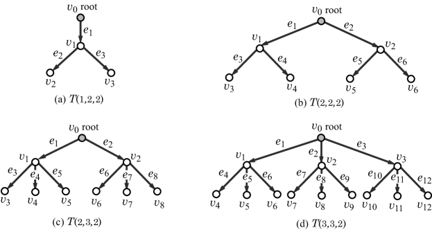
Figure 1: An illustration of rooted trees $T(a,b,c)$: (a) $T(1,2,2)$; (b)$T(2,2,2)$; (c) $T(2,3,2)$; (d) $T(3,3,2)$.

Branch-height in Trees Azam et al. [4] introduced “branch-height” of a tree as a new measure to the “agglomeration degree” of trees. We specify a non-negative integer ${\rho}$, called a branch-parameter to define branch-height. First we regard $T$ as a rooted tree by choosing the center of $T$ as the root.

We introduce the following terminology on a rooted tree $T$.

• A leaf ${\rho}$-branch: a non-root vertex $v$ in $T$ such that $\mathrm{height}(v)={\rho}$.

• A non-leaf ${\rho}$-branch: a vertex $v$ in $T$ such that $v$ has at least two children $u$ with $\mathrm{height}(u)\geq{\rho}$. We call a leaf or non-leaf ${\rho}$-branch a ${\rho}$-branch.

• A ${\rho}$-branch-path: a path $P$ in $T$ that joins two vertices $u$ and $u^{\prime}$ such that each of $u$ and $u^{\prime}$ is the root or a ${\rho}$-branch and $P$ does not contain the root or a ${\rho}$-branch as an internal vertex.

• The ${\rho}$-branch-subtree of $T$: the subtree of $T$ that consists of the edges in all ${\rho}$-branch-paths of $T$. We call a vertex (resp., an edge) in $T$ a ${\rho}$-internal vertex (resp., a ${\rho}$-internal edge) if it is contained in the ${\rho}$-branch-subtree of $T$ and a ${\rho}$-external vertex (resp., a ${\rho}$-external edge) otherwise. Let $V^{\mathrm{in}}$ and $V^{\mathrm{ex}}$ (resp., $E^{\mathrm{in}}$ and $E^{\mathrm{ex}}$) denote the sets of ${\rho}$-internal and ${\rho}$-external vertices (resp., edges) in $T$.

• The ${\rho}$-branch-tree of $T$: the rooted tree obtained from the ${\rho}$-branch-subtree of $T$ by replacing each ${\rho}$-branch-path with a single edge.

• A ${\rho}$-fringe-tree: One of the connected components that consists of the edges not in any ${\rho}$-branch-subtree. Each ${\rho}$-fringe-tree $T^{\prime}$ contains exactly one vertex $v$ in a ${\rho}$-branch-subtree, where $T^{\prime}$ is regarded as a tree rooted at $v$. Note that the height of any ${\rho}$-fringe-tree is at most ${\rho}$.

• The ${\rho}$-branch-number $\mathrm{bn}_{\rho}(T)$: the number of ${\rho}$-branches in $T$.

• The ${\rho}$-branch-height $\mathrm{bh}_{\rho}(T)$ of $T$: the maximum number of non-root ${\rho}$-branches along a path from the root to a leaf of $T$; i.e., $\mathrm{bh}_{\rho}(T)$ is the height of the ${\rho}$-branch-tree $T^{*}$ (the maximum length of a path from the root to a leaf in $T^{*}$).

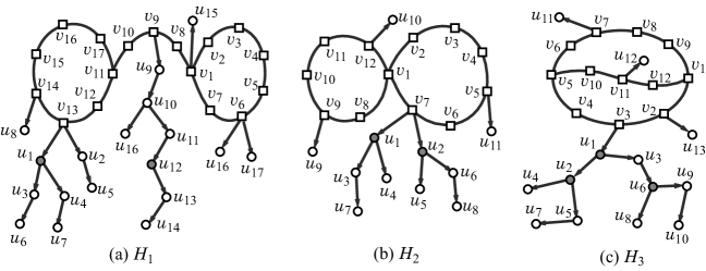
Figure 2: An illustration of rank-2 graphs $H_{i}$, $i=1,2,3$, where the core-vertices are depicted wtih squares, the $2$-branch vertices are depicted with gray circles and non-core edges are depicted as directed edges with arrows: (a) $H_{1}$ is 2-lean, $\mathrm{cs}(H_{1})=17$, $\mathrm{ch}(H_{1})=6$, $\mathrm{bh}_{2}(H_{1})=1$ and $\mathrm{bc}(H_{1})_{2}=\mathrm{bl}_{2}(H_{1})=2$; (b) $H_{2}$ is not 2-lean, $\mathrm{cs}(H_{2})=12$, $\mathrm{ch}(H_{2})=3$, $\mathrm{bh}_{2}(H_{2})=1$, $\mathrm{bc}_{2}(H_{2})=1$ and $\mathrm{bl}_{2}(H_{2})=2$; (c) $H_{3}$ is not 2-lean, $\mathrm{cs}(H_{3})=12$, $\mathrm{ch}(H_{3})=5$, $\mathrm{bh}_{2}(H_{3})=2$, $\mathrm{bc}_{2}(H_{3})=1$ and $\mathrm{bl}_{2}(H_{3})=2$.

Core in Cyclic Graphs Let $H$ be a connected simple graph with rank $\mathrm{r}(H)\geq 1$.

The core $\mathrm{Cr}(H)$ of $H$ is defined to be an induced subgraph $\mathrm{Cr}(H)=(V^{\prime}=V^{\prime}_{1}\cup V^{\prime}_{2},E^{\prime})$ such that $V^{\prime}_{1}$ is the set of vertices in a cycle of $H$ and $V^{\prime}_{2}$ is the set of verices each of which is in a path between two vertices $u,v\in V^{\prime}_{1}$. A vertex (resp., an edge) in $H$ is called a core-vertex (resp., core-edge) if it is contained in the core $\mathrm{Cr}(H)$ and is called a non-core-vertex (resp., non-core-edge) otherwise. We denote by $V^{\mathrm{co}}$ (resp., $V^{\mathrm{nc}}$) and $E^{\mathrm{co}}$ (resp., $E^{\mathrm{nc}}$) the set of core-vertices (resp., non-core-vertices) and the set of core-edges (resp., non-core-edges) in $H$. The core size $\mathrm{cs}(H)$ is defined to be the number $|V^{\mathrm{co}}|$ of core-vertices in the core of $H$.

Figure 2 illustrates three examples of rank-2 graphs $H_{i}$, $i=1,2,3$ and Figure 3 illustrates their cores $\mathrm{Cr}(H_{i})$, where $\mathrm{cs}(H_{1})=17$, $\mathrm{ch}(H_{1})=6$, $\mathrm{cs}(H_{2})=12$, $\mathrm{ch}(H_{2})=3$, $\mathrm{cs}(H_{3})=12$ and $\mathrm{ch}(H_{3})=5$.

A connected component in the subgraph induced by the non-core-vertices of $H$ is called a non-core component of $H$. Each non-core component $T$ contains exactly one non-core-vertex $v_{T}\in V^{\mathrm{nc}}$ that is adjacent to a core-vertex $u_{T}\in V^{\mathrm{co}}$, where the tree $T^{\prime}$ that consists of $T$ and edge $v_{T}u_{T}\in E^{\mathrm{nc}}$ is called a pendant-tree of $H$ regarded as a tree rooted at the core-vertex $u_{T}$. The core height $\mathrm{ch}(H)$ is defined to be the maximum height $\mathrm{ht}(T)$ of a pendant-tree $T$ of $H$.

A core-path $P$ of a graph $H$ is defined to be a subgraph of the core $\mathrm{Cr}(H)=(V^{\mathrm{co}},E^{\mathrm{co}})$ such that the degree of each internal vertex $v$ of $P$ is 2 in the core; i.e., $\deg_{P}(v)=\deg_{\mathrm{Cr}(H)}(v)=2$. A path-partition $\mathcal{P}$ of the core $\mathrm{Cr}(H)$ is defined to be a collection of core-paths $P_{i}$ with $\ell(P_{i})\geq 1$, $i=[1,p]$ such that each core-edge belongs to exactly one core-path in $\mathcal{P}$; i.e.,

$$\bigcup_{i\in[1,p]}E(P_{i})=E^{\mathrm{co}},~{}~{}E(P_{i})\cap E(P_{j})=\emptyset,1\leq i<j\leq p.$$

For example, the core $\mathrm{Cr}(H_{1})$ in Figure 2(a) admits a path-partition $\mathcal{P}=\{P_{1},P_{2},\ldots,P_{5}\}$ such that $P_{1}=(v_{1},v_{2},v_{3},v_{4},v_{5})$, $P_{2}=(v_{1},v_{7},v_{6},v_{5})$, $P_{3}=(v_{1},v_{8},v_{9},v_{10},v_{11})$, $P_{4}=(v_{11},v_{12},v_{13},v_{14},v_{15})$ and $P_{5}=(v_{15},v_{16},v_{17},v_{11})$.

Branch-height in Cyclic Graphs Let $H$ be a connected simple graph with rank $\mathrm{r}(H)\geq 1$.

For a branch parameter ${\rho}\geq 0$, we define ${\rho}$-fringe-tree, leaf ${\rho}$-branch, ${\rho}$-branch, ${\rho}$-branch-path, ${\rho}$-branch-subtree, ${\rho}$-internal/${\rho}$-external vertex/edges, ${\rho}$-branch-tree and ${\rho}$-branch-height in each pendant-tree of $H$ analogously, where we do not regard any core-vertex as a ${\rho}$-branch. A non-core-vertex (resp., non-core-edge) in $H$ is called a ${\rho}$-internal vertex (resp., edge) or a ${\rho}$-external vertex (resp., edge) if it is in some ${\rho}$-fringe-tree of $H$. Let $V^{\mathrm{in}}$ and $V^{\mathrm{ex}}$ (resp., $E^{\mathrm{in}}$ and $E^{\mathrm{ex}}$) denote the sets of ${\rho}$-internal and ${\rho}$-external vertices (resp., edges) in $H$, where $V^{\mathrm{nc}}=V^{\mathrm{in}}\cup V^{\mathrm{ex}}$ and $E^{\mathrm{nc}}=E^{\mathrm{in}}\cup E^{\mathrm{ex}}$.

Define the ${\rho}$-branch-leaf-number $\mathrm{bl}_{\rho}(H)$ of $H$ to the number of leaf ${\rho}$-branches in $H$ and the ${\rho}$-branch-height $\mathrm{bh}_{\rho}(H)$ to be the maximum ${\rho}$-branch-height $\mathrm{bh}_{\rho}(T)$ over all pendant-trees $T$ of $H$. We call a pendant-tree of $H$ a ${\rho}$-pendant-tree if it contains at least one ${\rho}$-branch. We call a core-vertex adjacent to a ${\rho}$-pendant-tree a ${\rho}$-branch-core-vertex, denote by $V_{\rho}^{\mathrm{bc}}$ the set of ${\rho}$-branch-core-vertices and define the ${\rho}$-branch-core-size $\mathrm{bc}_{\rho}(H)$ to be $|V_{\rho}^{\mathrm{bc}}|$. Note that $\mathrm{cs}(H)\geq\mathrm{bc}_{\rho}(H)$, $\mathrm{bl}_{\rho}(H)\geq\mathrm{bc}_{\rho}(H)$ and either ${\rho}>\mathrm{ch}(H)$ or ${\rho}\leq\mathrm{ch}(H)=\mathrm{bh}_{\rho}(H)+{\rho}$.

We call a graph $H$ ${\rho}$-lean if $\mathrm{bl}_{\rho}(H)=\mathrm{bc}_{\rho}(H)$; i.e., all ${\rho}$-branches in $H$ are leaf ${\rho}$-branches and no two ${\rho}$-pendant-trees share the same ${\rho}$-branch-core-vertex. Note that the ${\rho}$-branch height of any ${\rho}$-lean graph is at most 1. Figure 2 illustrates three examples of rank-2 graphs. In the first example, $u_{1}$ and $u_{12}$ are the leaf 2-branches, $v_{13}$ and $v_{9}$ are the $2$-branch-core-vertices, $\mathrm{bc}_{2}(H_{1})=\mathrm{bl}_{2}(H_{1})=2$ holds and $H_{1}$ is $2$-lean. In the second example, $u_{1}$ and $u_{2}$ are the leaf 2-branches, $v_{7}$ is the $2$-branch-core-vertex, $\mathrm{bc}_{2}(H_{2})=1<\mathrm{bl}_{2}(H_{2})=2$ holds and $H_{2}$ is not 2-lean. In the third example, $u_{2}$ and $u_{6}$ are the leaf 2-branches, $u_{1}$ is the non-leaf 2-branch, $v_{3}$ is the $2$-branch-core-vertex, $\mathrm{bc}_{2}(H_{3})=1<\mathrm{bl}_{2}(H_{3})=2$ holds and $H_{3}$ is not $2$-lean.

We here show some statical feature of the chemical graphs in PubChem in terms of rank of graphs and ${\rho}$-branch height (see [4] for more details).

1. Nearly 87% (resp., 99%) of rank-4 chemical compounds with up to 100 non-hydrogen atoms in PubChem have the maximum degree 3 (resp., 4) of non-core-vertices.

2. Nearly 84% of the chemical compounds in the chemical database PubChem have rank at most 4.

3. Over 87% (resp., 96%) of rank-1 or rank-2 (resp., rank-3 or rank-4) chemical compounds with up to 50 non-hydrogen atoms in PubChem have the $2$-branch height $\mathrm{bh}_{2}(G)$ at most 1.

4. Over 92% of 2-fringe-trees of chemical compounds with up to 100 non-hydrogen atoms in PubChem obey the following size constraint:

   $$n\leq 2d+2 T n d$$ for each 2-fringe-tree with vertices and children of the root. (1)

5. For ${\rho}=2$, nearly 97% of cyclic chemical compounds with up to 100 non-hydrogen atoms in PubChem are 2-lean.

Polymer Topology A multigraph is called a polymer topology if it is connected and the degree of every vertex is at least 3. Tezuka and Oike [25] pointed out that a classification of polymer topologies will lay a foundation for elucidation of structural relationships between different macro-chemical molecules and their synthetic pathways. For integers $r\geq 0$ and $d\geq 3$, let $\mathcal{PT}(r,d)$ denote the set of all rank-$r$ polymer topologies with maximum degree at most $d$. For example, there are three polymer topologies in $\mathcal{PT}(2,4)$, as illustrated in Figure 3(d)-(f).

The polymer topology $\mathrm{Pt}(H)$ of a multigraph $H$ with $\mathrm{r}(H)\geq 2$ is defined to be a multigraph $H^{\prime}$ of degree at least 3 that is obtained from the core $\mathrm{Cr}(H)$ by contracting all vertices of degree 2. Note that $\mathrm{r}(\mathrm{Pt}(H))=\mathrm{r}(H)$.

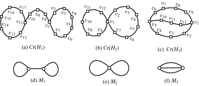
Figure 3: An illustration of rank-2 graphs and rank-2 multigraphs: (a), (b), (c) the cores $\mathrm{Cr}(H_{i})$, $i=1,2,3$ of the rank-2 graphs $H_{i}$, $i=1,2,3$ in Figure 2; (d), (e), (f) the three polymer topologies $M_{i}\in\mathcal{PT}(2,4)$, $i=1,2,3$, where $M_{i}\simeq\mathrm{Pt}(H_{i})$.

2.2 Modeling of Chemical Compounds

We represent the graph structure of a chemical compound as a graph $H$ with labels on vertices and multiplicity on edges in a hydrogen-suppressed model. We treat a cyclic graph $H$ as a mixed graph (a graph possibly with undirected and directed edges) by regarding each non-core-edge $uv\in E^{\mathrm{nc}}$ as a directed edge $(u,v)$ such that $u$ is the parent of $v$ in some pendant-tree of $H$. Each of the examples of rank-2 graphs in Figure 2 is represented as a mixed graph where non-core-edges are regarded as directed edges.

Let $\Lambda$ be a set of labels each of which represents a chemical element such as C (carbon), O (oxygen), N (nitrogen) and so on, where we assume that $\Lambda$ does not contain H (hydrogen). Let $\mathrm{mass}({\tt a})$ and $\mathrm{val}({\tt a})$ denote the mass and valence of a chemical element ${\tt a}\in\Lambda$, respectively. In our model, we use integers $\mathrm{mass}^{*}({\tt a})=\lfloor 10\cdot\mathrm{mass}({\tt a})\rfloor$, ${\tt a}\in\Lambda$ and assume that each chemical element ${\tt a}\in\Lambda$ has a unique valence $\mathrm{val}({\tt a})\in[1,4]$.

We introduce a total order $<$ over the elements in $\Lambda$ according to their mass values; i.e., we write ${\tt a<b}$ for chemical elements ${\tt a,b}\in\Lambda$ with $\mathrm{mass}({\tt a})<\mathrm{mass}({\tt b})$. To represent how two atoms ${\tt a}$ and ${\tt b}$ are joined in a chemical graph, we define some notions. A tuple $({\tt a},{\tt b},m)$ with chemical elements ${\tt a},{\tt b}$ and a bond-multiplicity $m$, called an adjacency-configuration was used to represent a pair of atoms ${\tt a}$ and ${\tt b}$ joined by a bond-multiplicity $m$ [6]. In this paper, we introduce “edge-configuration,” a refined notion of adjacency-configuration.

We represent an atom ${\tt a}\in\Lambda$ with $i$ neighbors in a chemical compound by a pair $({\tt a},i)$ of the chemical element ${\tt a}$ and the degree $i$, which we call a chemical symbol. For a notational convenience, we write a chemical symbol $({\tt a},i)$ (resp., $({\tt a},i+j)$) as ${\tt a}i$ (resp., ${\tt a}\{i+j\}$). Define the set of the chemical symbols to be

$$\Lambda_{\mathrm{dg}}(\Lambda,\mathrm{val})\triangleq\{{\tt a}i\mid{\tt a}\in\Lambda,i\in[1,\mathrm{val}({\tt a})]\}.$$

We extend the total order $<$ over $\Lambda$ to one over the elements in $\Lambda_{\mathrm{dg}}(\Lambda,\mathrm{val})$ so that ${\tt a}i<{\tt b}j$ if and only if “${\tt a}<{\tt b}$” or “${\tt a}={\tt b}$ and $i<j$.”

To represent how two atoms ${\tt a}$ and ${\tt b}$ are joined in a chemical compound, we use a tuple $({\tt a}i,{\tt b}j,m)$, ${\tt a}i,{\tt b}j\in\Lambda_{\mathrm{dg}}(\Lambda,\mathrm{val})$, $m\in[1,3]$ such that $i$ (resp., $j$) are the number of neighbors of the atom ${\tt a}$ (resp., ${\tt b}$) and $m$ is the bond-multiplicity between these atoms. We call the tuple $({\tt a}i,{\tt b}j,m)$ the edge-configuration of the pair of adjacent atoms. Let $\Lambda_{\mathrm{dg}}^{\prime}$ be a subset of $\Lambda_{\mathrm{dg}}(\Lambda,\mathrm{val})$. We denote by $\Gamma(\Lambda_{\mathrm{dg}}^{\prime})$ ‘ the set of all tuples $\gamma=({\tt a}i,{\tt b}j,m)\in\Lambda_{\mathrm{dg}}^{\prime}\times\Lambda_{\mathrm{dg}}^{\prime}\times[1,3]$ such that

$$m\leq\min\{\mathrm{val}({\tt a})-i,\mathrm{val}({\tt b})-j\}.$$

For a tuple $\gamma=({\tt a}i,{\tt b}j,m)\in\Gamma(\Lambda_{\mathrm{dg}}^{\prime})$, let $\overline{\gamma}$ denote the tuple $({\tt b}j,{\tt a}i,m)$. Define sets

$$\Gamma_{<}(\Lambda_{\mathrm{dg}}^{\prime})\triangleq\{\gamma=({\tt a}i,{\tt b}j,m)\in\Gamma(\Lambda_{\mathrm{dg}}^{\prime})\mid{\tt a}i<{\tt b}j\},$$

$$\Gamma_{=}(\Lambda_{\mathrm{dg}}^{\prime})\triangleq\{\gamma=({\tt a}i,{\tt b}j,m)\in\Gamma(\Lambda_{\mathrm{dg}}^{\prime})\mid{\tt a}i={\tt b}j\},$$

$$\Gamma_{>}(\Lambda_{\mathrm{dg}}^{\prime})\triangleq\{\gamma=({\tt a}i,{\tt b}j,m)\in\Gamma(\Lambda_{\mathrm{dg}}^{\prime})\mid{\tt a}i>{\tt b}j\}.$$

As components of a chemical graph to be inferred, we choose sets

$$\Lambda_{\mathrm{dg}}^{\mathrm{co}}\subseteq\Lambda_{\mathrm{dg}}(\Lambda,\mathrm{val}),~{}~{}~{}\Lambda_{\mathrm{dg}}^{\mathrm{nc}}\subseteq\Lambda_{\mathrm{dg}}(\Lambda,\mathrm{val}),$$

$$\Gamma^{\mathrm{co}}\subseteq\Gamma_{<}(\Lambda_{\mathrm{dg}}^{\mathrm{co}})\cup\Gamma_{=}(\Lambda_{\mathrm{dg}}^{\mathrm{co}}),~{}~{}\Gamma^{\mathrm{nc}}\subseteq\Gamma(\Lambda_{\mathrm{dg}}^{\mathrm{nc}})$$

such that $i\geq 2$ for any symbol ${\tt a}i\not\in\Lambda_{\mathrm{dg}}^{\mathrm{co}}$, where the degree of any vertex in the core of a cyclic graph is at least 2.

Let $e=uv$ be an edge in a chemical graph $G$ such that ${\tt a},{\tt b}\in\Lambda$ are assigned to the vertices $u$ and $v$ with $\deg_{G}(u)=i$ and $\deg_{G}(v)=j$, respectively and the bond-multiplicity between them is $m$. When $uv$ is a core-edge which is regarded as an undirected edge, the edge-configuration $\tau(e)$ of edge $e$ is defined to be $({\tt a}i,{\tt b}j,m)$ if $({\tt a}i,{\tt b}j,m)\in\Gamma^{\mathrm{co}}$ (or $({\tt b}j,{\tt a}i,m)$ otherwise). When $uv$ is a non-core-edge which is regarded as a directed edge $(u,v)$ where $u$ is the parent of $v$ in some pendant-tree, the edge-configuration $\tau(e)$ of edge $e$ is defined to be $({\tt a}i,{\tt b}j,m)\in\Gamma^{\mathrm{nc}}$.

When a branch-parameter ${\rho}$ is specified, we choose sets

$$\Gamma^{\mathrm{in}}\subseteq\Gamma^{\mathrm{nc}},~{}~{}~{}\Gamma^{\mathrm{ex}}\subseteq\Gamma^{\mathrm{nc}}$$

such that $i,j\geq 2$ for any tuple $({\tt a}i,{\tt b}j,m)\not\in\Gamma^{\mathrm{in}}$, where the degree of any ${\rho}$-internal vertex is at least 2.

We use a hydrogen-suppressed model because hydrogen atoms can be added at the final stage. A chemical cyclic graph over $\Lambda$ and $\Gamma=\Gamma^{\mathrm{co}}\cup\Gamma^{\mathrm{nc}}$ is defined to be a tuple $G=(H,\alpha,\beta)$ of a cyclic graph $H=(V,E)$, a function $\alpha:V\to\Lambda$ and a function $\beta:E\to[1,3]$ such that

1. $H$ is connected;

2. $\sum_{uv\in E}\beta(uv)\leq\mathrm{val}(\alpha(u))$ for each vertex $u\in V$; and

3. $\tau(e)\in\Gamma^{\mathrm{co}}$ for each core-edge $e\in E$; and $\tau(e)\in\Gamma^{\mathrm{nc}}$ for each directed non-core-edge $e\in E$.

For a notational convenience, we denote the sum of bond-multiplicities of edges incident to a vertex $u$ as follows:

$$\beta(u)\triangleq\sum_{uv\in E}\beta(uv)\mbox{ for each vertex $u\in V$.}$$

When a branch-parameter ${\rho}$ is given, the condition (iii) is given as follows.
   $\tau(e)\in\Gamma^{\mathrm{co}}$ for each core-edge $e\in E$;
   $\tau(e)\in\Gamma^{\mathrm{in}}$ for each directed ${\rho}$-internal non-core-edge $e\in E$; and
   $\tau(e)\in\Gamma^{\mathrm{ex}}$ for each directed ${\rho}$-external non-core-edge $e\in E$.

We represent the graph structure of a chemical compound as a graph with labels on vertices and multiplicity on edges in a hydrogen-suppressed model.

2.3 Descriptors

In our method, we use only graph-theoretical descriptors for defining a feature vector, which facilitates our designing an algorithm for constructing graphs. We choose a branch-parameter ${\rho}\geq 1$, sets $\Lambda_{\mathrm{dg}}^{\mathrm{co}}$ and $\Lambda_{\mathrm{dg}}^{\mathrm{nc}}$ of chemical symbols and sets $\Gamma^{\mathrm{co}},\Gamma^{\mathrm{in}}$ and $\Gamma^{\mathrm{ex}}$ of edge-configurations. Let $G=(H=(V,E),\alpha,\beta)$ be a chemical cyclic graph with the chemical symbols and the edge-configurations.

We define a feature vector $f(G)$ that consists of the following 16 kinds of descriptors.

• $n(G)$: the number $|V|$ of vertices.

• $\mathrm{cs}(G)$: the core size of $G$.

• $\mathrm{ch}(G)$: the core height of $G$.

• $\mathrm{bl}_{{\rho}}(G)$: the ${\rho}$-branch-leaf-number of $G$.

• $\overline{\mathrm{ms}}(G)$: the average mass^∗ of atoms in $G$; i.e., $\overline{\mathrm{ms}}(G)\triangleq\sum_{v\in V}\mathrm{mass}^{*}(\alpha(v))/n(G)$.

• $\mathrm{dg}_{i}^{\mathrm{co}}(G)$, $i\in[1,4]$: the number of core-vertices of degree $i$ in $G$;
      i.e., $\mathrm{dg}_{i}^{\mathrm{co}}(G)\triangleq|\{v\in V^{\mathrm{co}}\mid\deg_{H}(v)=i\}|$.

• $\mathrm{dg}_{i}^{\mathrm{nc}}(G)$, $i\in[1,4]$: the number of non-core-vertices of degree $i$ in $G$;
      i.e., $\mathrm{dg}_{i}^{\mathrm{nc}}(G)\triangleq|\{v\in V^{\mathrm{nc}}\mid\deg_{H}(v)=i\}|$.

• $\mathrm{bd}_{m}^{\mathrm{co}}(G)$, $m\in[2,3]$: the number of core-edges with bond multiplicity $m$;
      i.e., $\mathrm{bd}_{m}^{\mathrm{co}}(G)\triangleq\{e\in E^{\mathrm{co}}\mid\beta(e)=m\}$.

• $\mathrm{bd}_{m}^{\mathrm{in}}(G)$, $m\in[2,3]$: the number of ${\rho}$-internal edges with bond multiplicity $m$;
      i.e., $\mathrm{bd}_{m}^{\mathrm{in}}(G)\triangleq\{e\in E^{\mathrm{in}}\mid\beta(e)=m\}$.

• $\mathrm{bd}_{m}^{\mathrm{ex}}(G)$, $m\in[2,3]$: the number of ${\rho}$-external edges with bond multiplicity $m$;
      i.e., $\mathrm{bd}_{m}^{\mathrm{ex}}(G)\triangleq\{e\in E^{\mathrm{ex}}\mid\beta(e)=m\}$.

• $\mathrm{ns}_{\mu}^{\mathrm{co}}(G)$, $\mu\in\Lambda_{\mathrm{dg}}^{\mathrm{co}}$: the number of core-vertices $v$ with $\alpha(v)={\tt a}$ and $\deg_{G}(v)=i$ for $\mu={\tt a}i$.

• $\mathrm{ns}_{\mu}^{\mathrm{nc}}(G)$, $\mu\in\Lambda_{\mathrm{dg}}^{\mathrm{nc}}$: the number of non-core-vertices $v$ with $\alpha(v)={\tt a}$ and $\deg_{G}(v)=i$ for $\mu={\tt a}i$.

• $\mathrm{ec}_{\gamma}^{\mathrm{co}}(G)$, $\gamma\in\Gamma^{\mathrm{nc}}$: the number of undirected core-edges $e\in E^{\mathrm{co}}$ such that $\tau(e)=\gamma$.

• $\mathrm{ec}_{\gamma}^{\mathrm{in}}(G)$, $\gamma\in\Gamma^{\mathrm{in}}$: the number of directed ${\rho}$-internal edges $e\in E^{\mathrm{in}}$ such that $\tau(e)=\gamma$.

• $\mathrm{ec}_{\gamma}^{\mathrm{ex}}(G)$, $\gamma\in\Gamma^{\mathrm{ex}}$: the number of directed ${\rho}$-external edges $e\in E^{\mathrm{ex}}$ with $\tau(e)=\gamma$.

• $\mathrm{ns}_{\tt H}(G)$: the number of hydrogen atoms; i.e., $\displaystyle{\mathrm{ns}_{\tt H}(G)\triangleq\sum_{v\in V}\mathrm{val}(\alpha(v))-2\sum_{e\in E}\beta(e).}$

The number $K$ of descriptors in our feature vector $x=f(G)$ is $K=|\Lambda_{\mathrm{dg}}^{\mathrm{co}}|+|\Lambda_{\mathrm{dg}}^{\mathrm{nc}}|+|\Gamma^{\mathrm{co}}|+|\Gamma^{\mathrm{in}}|+|\Gamma^{\mathrm{co}}|+20$. Note that the set of the above $K$ descriptors is not independent in the sense that some descriptor depends on the combination of other descriptors in the set. For example, descriptor $\mathrm{bd}_{m}^{\mathrm{ex}}(G)$ can be determined by $\sum_{\gamma=(\mu,\mu^{\prime},i)\in\Gamma:i=m}\mathrm{ec}_{\gamma}^{\mathrm{ex}}(G)$.

3 A Method for Inferring Chemical Graphs

3.1 Framework for the Inverse QSAR/QSPR

We review the framework that solves the inverse QSAR/QSPR by using MILPs  [6, 11, 30], which is illustrated in Figure 4. For a specified chemical property $\pi$ such as boiling point, we denote by $a(G)$ the observed value of the property $\pi$ for a chemical compound $G$. As the first phase, we solve (I) Prediction Problem with the following three steps.

Phase 1.
Stage 1:  Let $\mathrm{DB}$ be a set of chemical graphs. For a specified chemical property $\pi$, choose a class $\mathcal{G}$ of graphs such as acyclic graphs or graphs with a given rank $r$. Prepare a data set $D_{\pi}=\{G_{i}\mid i=1,2,\ldots,m\}\subseteq\mathcal{G}\cap\mathrm{DB}$ such that the value $a(G_{i})$ of each chemical graph $G_{i}$, $i=1,2,\ldots,m$ is available. Set reals $\underline{a},\overline{a}\in\mathbb{R}$ so that $\underline{a}\leq a(G_{i})\leq\overline{a}$, $i=1,2,\ldots,m$.

Stage 2:  Introduce a feature function $f:\mathcal{G}\to\mathbb{R}^{K}$ for a positive integer $K$. We call $f(G)$ the feature vector of $G\in\mathcal{G}$, and call each entry of a vector $f(G)$ a descriptor of $G$.

Stage 3:  Construct a prediction function $\psi_{\mathcal{N}}$ with an ANN $\mathcal{N}$ that, given a vector in $\mathbb{R}^{K}$, returns a real in the range $[\underline{a},\overline{a}]$ so that $\psi_{\mathcal{N}}(f(G))$ takes a value nearly equal to $a(G)$ for many chemical graphs in $D$.

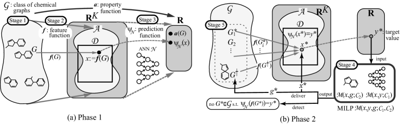
Figure 4: (a) An illustration of Phase 1: Stage 1 for preparing a data set $D_{\pi}$ for a graph class $\mathcal{G}$ and a specified chemical property $\pi$; Stage 2 for introducing a feature function $f$ with descriptors; Stage 3 for constructing a prediction function $\psi_{\mathcal{N}}$ with an ANN $\mathcal{N}$; (b) An illustration of Phase 2: Stage 4 for formulating an MILP $\mathcal{M}(x,y,g;\mathcal{C}_{1},\mathcal{C}_{2})$ and finding a feasible solution $(x^{*},g^{*})$ of the MILP for a target value $y^{*}$ so that $\psi_{\mathcal{N}}(x^{*})=y^{*}$ (possibly detecting that no target graph $G^{*}$ exists); Stage 5 for enumerating graphs $G^{*}\in\mathcal{G}$ such that $f(G^{*})=x^{*}$.

See Figure 4(a) for an illustration of Stages 1, 2 and 3 in Phase 1.

For the set of descriptors $\kappa_{j}$, $j\in[1,K]$ in a feature vector $x\in\mathbb{R}^{K}$, we can choose lower and upper bounds $\kappa_{j}^{\mathrm{LB}}$ and $\kappa_{j}^{\mathrm{UB}}$ on each descriptor $\kappa_{j}$, and denote by $\mathcal{D}$ the set of vectors $x\in\mathbb{R}^{K}$ such that $\kappa_{j}^{\mathrm{LB}}\leq x_{j}\leq\kappa_{j}^{\mathrm{UB}}$, $j\in[1,K]$. For example, we can use the range-based method to define an applicability domain (AD) [18] to inverse QSAR/QSPR by using such a restricted set $\mathcal{D}$. Compute the minimum value $\underline{x_{j}}$ and the maximum value $\overline{x_{j}}$ of the $j$-th descriptor $x_{j}$ in $f(G_{i})$ over all graphs $G_{i}$, $i=1,2,\ldots,m$ in a data set $D_{\pi}$. Choose lower and upper bounds $\kappa_{j}^{\mathrm{LB}}$ and $\kappa_{j}^{\mathrm{UB}}$ so that $\underline{x_{j}}\leq\kappa_{j}^{\mathrm{LB}}$ and $\kappa_{j}^{\mathrm{UB}}\leq\overline{x_{j}}$, $j\in[1,K]$.

In the second phase, we try to find a vector $x^{*}\in\mathbb{R}^{K}$ from a target value $y^{*}$ of the chemical propery $\pi$ such that $\psi_{\mathcal{N}}(x^{*})=y^{*}$. Based on the method due to Akutsu and Nagamochi [2], Chiewvanichakorn et al. [6] showed that this problem can be formulated as an MILP. By including a set of linear constraints such that $x\in\mathcal{D}$ into their MILP, we obtain the next result.

Theorem 1.

([11, 30]) Let $\mathcal{N}$ be an ANN with a piecewise-linear activation function for an input vector $x\in\mathbb{R}^{K}$, $n_{A}$ denote the number of nodes in the architecture and $n_{B}$ denote the total number of break-points over all activation functions. Then there is an MILP $\mathcal{M}(x,y;\mathcal{C}_{1})$ that consists of variable vectors $x\in\mathcal{D}~{}(\subseteq\mathbb{R}^{K})$, $y\in\mathbb{R}$, and an auxiliary variable vector $z\in\mathbb{R}^{p}$ for some integer $p=O(n_{A}+n_{B})$ and a set $\mathcal{C}_{1}$ of $O(n_{A}+n_{B})$ constraints on these variables such that: $\psi_{\mathcal{N}}(x^{*})=y^{*}$ if and only if there is a vector $(x^{*},y^{*})$ feasible to $\mathcal{M}(x,y;\mathcal{C}_{1})$.

In the second phase, we solve (II) Inverse Problem, wherein given a target chemical value $y^{*}$, we are asked to generate chemical graphs $G^{*}\in\mathcal{G}$ such that $f(G^{*})=x^{*}$. For this, we first find a vector $x^{*}\in\mathbb{R}^{K}$ such that $\psi_{\mathcal{N}}(x^{*})=y^{*}$ and then generate chemical graphs $G^{*}\in\mathcal{G}$ such that $f(G^{*})=x^{*}$. However, the resulting vector $x^{*}$ may not admit such a chemical graph $G^{*}\in\mathcal{G}$. Azam et al. [3] called a vector $x\in\mathbb{R}^{K}$ admissible if there is a graph $G\in\mathcal{G}$ such that $f(G)=x$. Let $\mathcal{A}$ denote the set of admissible vectors $x\in\mathbb{R}^{K}$. To ensure that a vector $x^{*}$ inferred from a given target value $y^{*}$ becomes admissible, we introduce a new vector variable $g\in\mathbb{R}^{q}$ for an integer $q$ so that a feasible solution $(x^{*},g^{*})$ of the MILP for a target value $y^{*}$ delivers a vector $x^{*}$ with $\psi_{\mathcal{N}}(x^{*})=y^{*}$ and a vector $g^{*}$ that represents a chemical graph $G^{\dagger}\in\mathcal{G}$ with $f(G^{\dagger})=x^{*}$. In the second phase, we treat the next two problems.

(II-a) Inference of Vectors
Input: A real $y^{*}$ with $\underline{a}\leq y^{*}\leq\overline{a}$.
Output: Vectors $x^{*}\in\mathcal{A}\cap\mathcal{D}$ and $g^{*}\in\mathbb{R}^{q}$ such that $\psi_{\mathcal{N}}(x^{*})=y^{*}$ and $g^{*}$ forms a chemical graph $G^{\dagger}\in\mathcal{G}$ with $f(G^{\dagger})=x^{*}$.

(II-b) Inference of Graphs
Input: A vector $x^{*}\in\mathcal{A}\cap\mathcal{D}$.
Output: All graphs $G^{*}\in\mathcal{G}$ such that $f(G^{*})=x^{*}$.

The second phase consists of the next two steps.

Phase 2.
Stage 4:  Formulate Problem (II-a) as the above MILP $\mathcal{M}(x,y,g;\mathcal{C}_{1},\mathcal{C}_{2})$ based on $\mathcal{G}$ and $\mathcal{N}$. Find a feasible solution $(x^{*},g^{*})$ of the MILP such that

$$x^{*}\in\mathcal{A}\cap\mathcal{D} \psi_{\mathcal{N}}(x^{*})=y^{*}$$ and

(where the second requirement may be replaced with inequalities $(1-\varepsilon)y^{*}\leq\psi_{\mathcal{N}}(x^{*})\leq(1+\varepsilon)y^{*}$ for a tolerance $\varepsilon>0$).

Stage 5:  To solve Problem (II-b), enumerate all (or a specified number) of graphs $G^{*}\in\mathcal{G}$ such that $f(G^{*})=x^{*}$ for the inferred vector $x^{*}$.

See Figure 4(b) for an illustration of Stages 4 and 5 in Phase 2.

3.2 A New Mechanism for Stage 5

Execution of Stage 5; i.e. generating chemical graphs $G^{*}$ that satisfy $f(G^{*})=x^{*}$ for a given feature vector $x^{*}\in\mathbb{Z}_{+}^{K}$ is a challenging issue for a relatively large instance with size $n(G^{*})\geq 20$. There have been proposed algorithms for Stage 5 for classes of graphs with rank 0 to 2  [8, 24, 26, 27]. All of these are designed based on the branch-and-bound method where an enormous number of chemical graphs are constructed by repeatedly appending and removing a vertex one by one until a target chemical graph is constructed. These algorithms can generate a target chemical graph with size $n(G^{*})\leq 20$. To break this barrier, Azam et al. [4] recently employed the dynamic programming method for designing a new algorithm in Stage 5 and showed that chemical acyclic graphs $G^{*}$ with a bounded branch-height can be generated for size $n(G^{*})=50$. However, for a class of graphs with a different rank, we may need to design again a new algorithm by the dynamic programming method. Moreover, algorithms for higher ranks can be more complicated and do not run as fast as the algorithm for acyclic graphs due to Azam et al. [4].

In this paper, as a new mechanism of Stage 5, we adopt an idea of utilizing the chemical graph $G^{\dagger}\in\mathcal{G}$ obtained as part of a feasible solution of an MILP in Stage 4. In other words, we modify the chemical graph $G^{\dagger}$ to generate other chemical graphs $G^{*}$ that are “chemically isomorphic” to $G^{\dagger}$ in the sense that $f(G^{*})=f(G^{\dagger})$ holds. Informally speaking, we reduce the problem of finding such a graph $G^{*}$ into a problem of generating chemical acyclic graphs, to which we have obtained an efficient dynamic programming algorithm [4]. We first decompose $G^{\dagger}$ into a collection of chemical trees $T^{\dagger}_{1},T^{\dagger}_{2},\ldots,T^{\dagger}_{m}$ such that for a subset $V_{B}$ of the core-vertices of $G^{\dagger}$, any tree $T^{\dagger}_{i}$ contains at most two vertices in $V_{B}$, as illustrated in Figure 5(a). Let $x^{*}_{i}$ denote the feature vector $f(T^{\dagger}_{i})$. For each index $i$, we generate chemical acyclic graphs $T^{*}_{i}$ such that $f(T^{*}_{i})=x^{*}_{i}$. Finally we combine the generated chemical trees $T^{*}_{1},T^{*}_{2},\ldots,T^{*}_{m}$ to construct a chemical cyclic graph $G^{*}$ such that $f(G^{*})=\sum_{i\in[1,m]}x^{*}_{i}=f(G^{\dagger})$. See Section 6 for the details. Although a family of chemical graphs $G^{*}$ chemically isomorphic to $G^{\dagger}$ depends on a choice of decomposition into trees $T^{\dagger}_{i}$ and covers only part of the entire set of target graphs $G^{*}$ with $f(G^{*})=x^{*}$, the new method can be applied to any class of graphs or even to a graph with a specific substructure.

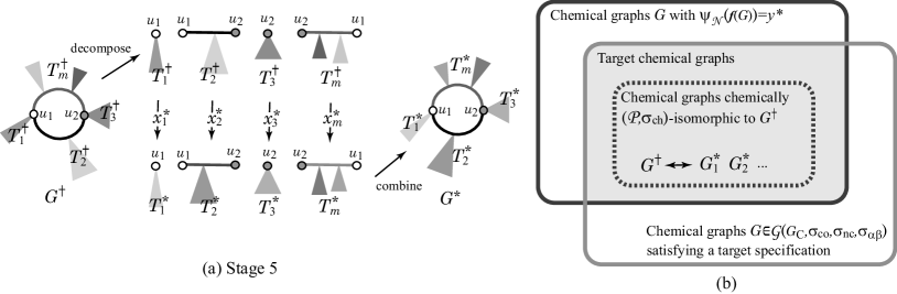
Figure 5: An illustration of a process of Stage 5 and a set of target isomorphic graphs: (a) A new mechanism to Stage 5, where a given target chemical graph $G^{\dagger}$ is decomposed into chemical trees $T^{\dagger}_{i}$, $i=1,2,\ldots,m$ into chemical trees $T^{\dagger}_{i}$, $i=1,2,\ldots,m$ based on a set $V_{B}=\{u_{1},u_{2}\}$ of core-vertices and for each feature vector $x^{*}_{i}=f(T^{\dagger}_{i})$, a chemical tree $T^{*}_{i}$ such that $f(T^{*}_{i})=x^{*}_{i}$ is constructed before a new target graph $G^{*}_{1}$ is obtained as a combination of the resulting chemical trees $T^{*}_{1},\ldots,T^{*}_{m}$; (b) Given a target value $y^{*}$, an MILP $\mathcal{M}(x,y,g;\mathcal{C}_{1},\mathcal{C}_{2})$ delivers a target chemical graph $G^{\dagger}$, if the intersection of the set of chemical graphs $G$ with $\psi_{\mathcal{N}}(f(G))=y^{*}$ and the set of chemical graphs $G$ that satisfy a target specification $(G_{\mathrm{C}},\sigma_{\mathrm{co}},\sigma_{\mathrm{nc}},\sigma_{\mathrm{\alpha\beta}})$ is not empty, where all chemically $(\mathcal{P},\sigma_{\mathrm{ch}})$-isomorphic graphs to $G^{\dagger}$ belong to the intersection.

3.3 A Flexible Specification to Target Chemical Graphs

In the previous application of the framework, a target chemical graph $G$ to be inferred is specified with a small number of parameters such as the number $n(G)$ of vertices, the core size $\mathrm{cs}(G)$ and the core height $\mathrm{ch}(G)$.

In this paper, we also introduce a more flexible way of specifying a target graph so that our new algorithm for generating chemically isomorphic graphs $G^{*}$ can be used. Suppose that we are given a requirement $R$ on a target graph specified other than the feature vector $f$. Now a target graph is defined to be a chemical graph $G$ that satisfies $\psi_{\mathcal{N}}(f(G))=y^{*}$ for a given target value $y^{*}$ and the requirement at the same time. In general, a chemical graph $G^{*}$ such that $f(G^{*})=f(G^{\dagger})$ may not satisfy such an additional requirement $R$. Recall that $G^{*}$ in Stage 5 is obtained as a combination of chemical trees $T^{*}_{i}$ each of which is chemically isomorphic to the corresponding tree $T^{\dagger}_{i}$ of the given graph $G^{\dagger}$. Hence if the requirement $R$ on a target chemical graph is independent among such chemical trees $T^{*}_{i}$ to be inferred from a vector $x^{*}_{i}$, then any combination $G^{*}$ of inferred chemical trees $T^{*}_{i}$ still satisfies the requirement $R$, whenever the original graph $G^{\dagger}$ satisfies $R$. See Figure 5(b) for an illustration of the set of chemical graphs $G^{*}$ that are chemically isomorphic to a target chemical graph $G^{\dagger}$. Section 4 describes a way of specifying a requirement, called a “target specification” such that a prescribed substructure of graphs such as a benzene ring to be included in a target chemical graph or a partly predetermined assignment of chemical elements and bond-multiplicity to a target graph.

4 Specifying Target Chemical Graphs

This section presents a flexible way of specifying a topological structure of the core and assignments of chemical elements and bond-multiplicity of a target chemical graph. We define a target specification $(G_{\mathrm{C}},\sigma_{\mathrm{co}},\sigma_{\mathrm{nc}},\sigma_{\mathrm{\alpha\beta}})$ with a multigraph $G_{\mathrm{C}}$ and sets $\sigma_{\mathrm{co}},\sigma_{\mathrm{nc}}$ and $\sigma_{\mathrm{\alpha\beta}}$ of lower and upper bounds on several descriptors that we describe in the following.

4.1 Seed Graphs

A seed graph $G_{\mathrm{C}}=(V_{\mathrm{C}},E_{\mathrm{C}})$ is defined to be a multigraph with no self-loops such that the edge set $E_{\mathrm{C}}$ consists of four sets $E_{(\geq 2)}$, $E_{(\geq 1)}$, $E_{(0/1)}$ and $E_{(=1)}$, where each of them can be empty. Figure 6 illustrates an example of a seed graph. From a seed graph $G_{\mathrm{C}}$, the core of a cyclic graph will be constructed in the following way:

1. Each edge $e=uv\in E_{(\geq 2)}$ will be replaced with a $u,v$-path $P_{e}$ of length at least 2.

2. Each edge $e=uv\in E_{(\geq 1)}$ will be replaced with a $u,v$-path $P_{e}$ of length at least 1 (equivalently $e$ is directly used or replaced with a $u,v$-path $P_{e}$ of length at least 2).

3. Each edge $e\in E_{(0/1)}$ is either used or discarded.

4. Each edge $e\in E_{(=1)}$ is always used directly.

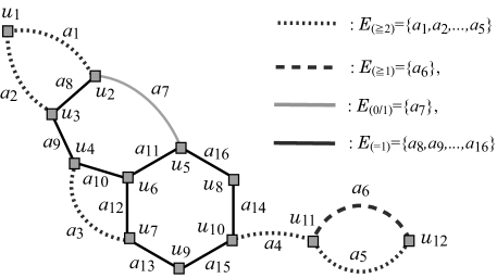
Figure 6: An illustration of a seed graph $G_{\mathrm{C}}$ with $E_{(\geq 2)}=\{a_{1},a_{2},\ldots,a_{5}\}$, $E_{(\geq 1)}=\{a_{6}\}$, $E_{(0/1)}=\{a_{7}\}$ and $E_{(=1)}=\{a_{8},a_{9},\ldots,a_{16}\}$, where the vertices in $V_{\mathrm{C}}$ are depicted with gray squares, the edges in $E_{(\geq 2)}$ are depicted with dotted lines, the edges in $E_{(\geq 1)}$ are depicted with dashed lines, the edges in $E_{(0/1)}$ are depicted with gray lines and the edges in $E_{(=1)}$ are depicted with black solid lines.

4.2 Core Specification

The core of a target chemical graph is constructed from a seed graph $G_{\mathrm{C}}$ by a core specification $\sigma_{\mathrm{co}}$ that consists of the following:

1. Lower and upper bound functions $\ell_{\mathrm{LB}},\ell_{\mathrm{UB}}:E_{(\geq 2)}\cup E_{(\geq 1)}\to\mathbb{Z}_{+}$. For a notational convenience, set $\ell_{\mathrm{LB}}(e):=0$, $\ell_{\mathrm{UB}}(e):=1$, $e\in E_{(0/1)}$ and $\ell_{\mathrm{LB}}(e):=1$, $\ell_{\mathrm{UB}}(e):=1$, $e\in E_{(=1)}$.

2. Lower and upper bounds $\mathrm{cs}_{\mathrm{LB}},\mathrm{cs}_{\mathrm{UB}}\in\mathbb{Z}_{+}$ on the core size, where we assume $\mathrm{cs}_{\mathrm{LB}}\geq|V_{\mathrm{C}}|+\sum_{e\in E_{(\geq 2)}\cup E_{(\geq 1)}}(\ell_{\mathrm{LB}}(e)-1)$.

3. Side constraints: As an option, we can specify additional linear constraints on the length $\ell(P_{i})$ of path $P_{i}$, $a_{i}\in E_{\mathrm{C}}$ such as $\ell(P_{2})+\ell(P_{3})=c$ for a constant $c$ or $\ell(P_{1})\leq\ell(P_{4})+\ell(P_{5})$.

An example of a core specification $\sigma_{\mathrm{co}}$ to the seed graph $G_{\mathrm{C}}$ in Figure 6 is given in Table 1.

Table 1: Example 1 of a core specification $\sigma_{\mathrm{co}}$.

	$a_{1}$	$a_{2}$	$a_{3}$	$a_{4}$	$a_{5}$	$a_{6}$
$\ell_{\mathrm{LB}}(a_{i})$	2	2	2	3	2	1
$\ell_{\mathrm{UB}}(a_{i})$	3	4	3	5	4	4

$\mathrm{cs}_{\mathrm{LB}}=20$

$\mathrm{cs}_{\mathrm{UB}}=28$

A $\sigma_{\mathrm{co}}$-extension of a seed graph $G_{\mathrm{C}}$ is defined to be a graph $C$ such that $|V(C)|\in[\mathrm{cs}_{\mathrm{LB}},\mathrm{cs}_{\mathrm{UB}}]$ and $C$ is obtained from replacing each edge $e=uv\in E_{(\geq 2)}\cup E_{(\geq 1)}$ with a $u,v$-path $P_{e}$ of length $\ell(P_{e})\in[\ell_{\mathrm{LB}}(e),\ell_{\mathrm{UB}}(e)]$ under specified side constraints, if any. Figure 7 illustrates one of the $\sigma_{\mathrm{co}}$-extensions of the seed graph $G_{\mathrm{C}}$ in Figure 6 with the core specification $\sigma_{\mathrm{co}}$ in Table 1. The edges $a_{i}\in E_{(\geq 2)}$, $i\in[1,5]$ are replaced with paths $P_{1}=(u_{1},u_{13},u_{3})$, $P_{2}=(u_{1},u_{14},u_{3})$, $P_{3}=(u_{4},u_{15},u_{16},u_{7})$, $P_{4}=(u_{10},u_{17},u_{18},u_{19},u_{11})$ and $P_{5}=(u_{11},u_{20},u_{21},u_{22},u_{12})$, respectively. The edge $a_{6}\in E_{(\geq 1)}$ is used in the graph $C$ and the edge $a_{7}\in E_{(0/1)}$ is discarded, where $E_{(=1)}\subseteq E(C)$.

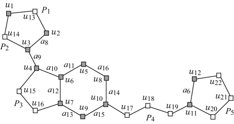
Figure 7: An illustration of a $\sigma_{\mathrm{co}}$-extension $C$ with $\mathrm{cs}(C)=22$, where the vertices in $V(C)\setminus V_{\mathrm{C}}$ are depicted with white squares.

Let $\mathcal{C}(G_{\mathrm{C}},\sigma_{\mathrm{co}})$ denote the set of all $\sigma_{\mathrm{co}}$-extensions of a seed graph $G_{\mathrm{C}}$. We employ a graph $C\in\mathcal{C}(G_{\mathrm{C}},\sigma_{\mathrm{co}})$ as the core $\mathrm{Cr}(G)$ of a chemical graph $G$ to be inferred.

Remember that the core of any connected cyclic graph is a simple connected graph with minimum degree at least 2. Possibly some $\sigma_{\mathrm{co}}$-extension of a seed graph $G_{\mathrm{C}}$ is not such a graph. We show some sufficient condition for any $\sigma_{\mathrm{co}}$-extension to be a simple connected graph with minimum degree at least 2. Let $C_{\min}\in\mathcal{C}(G_{\mathrm{C}},\sigma_{\mathrm{co}})$ denote the minimum $\sigma_{\mathrm{co}}$-extension; i.e., $C_{\min}$ is obtained from the graph $(V_{\mathrm{C}},E_{(\geq 2)}\cup E_{(\geq 1)}\cup E_{(=1)})$ by replacing each edge $e\in E_{(\geq 2)}$ with a path of the least length $\ell_{\mathrm{LB}}(e)$. We see that if $C_{\min}$ is a connected graph with minimum degree at least 2 then any extension $C\in\mathcal{C}(G_{\mathrm{C}},\sigma_{\mathrm{co}})$ becomes a simple connected graph with minimum degree at least 2.

4.3 Non-core Specification

Next we show how to specify the structure of the non-core part of a target chemical graph. For a seed graph $G_{\mathrm{C}}$, let a non-core specification $\sigma_{\mathrm{nc}}$ consist of the following:

1. Lower and upper bounds $n_{\mathrm{LB}},n^{*}\in\mathbb{Z}_{+}$ on the number of vertices, where $\mathrm{cs}_{\mathrm{LB}}\leq n_{\mathrm{LB}}\leq n^{*}$.

2. An upper bound $\mathrm{dg}^{\mathrm{nc}}_{4,\mathrm{UB}}\in\mathbb{Z}_{+}$ on the number of non-core-vertices of degree 4.

3. Lower and upper functions $\mathrm{ch}_{\mathrm{LB}},\mathrm{ch}_{\mathrm{UB}}:V_{\mathrm{C}}\to\mathbb{Z}_{+}$ and $\mathrm{ch}_{\mathrm{LB}},\mathrm{ch}_{\mathrm{UB}}:E_{(\geq 2)}\cup E_{(\geq 1)}\to\mathbb{Z}_{+}$ on the maximum height of trees rooted at a vertex $v\in V_{\mathrm{C}}$ or at an internal vertex of a path $P_{e}$ with $e\in E_{(\geq 2)}\cup E_{(\geq 1)}$.

4. A branch-parameter ${\rho}\in\mathbb{Z}_{+}$.

5. Lower and upper functions $\mathrm{bl}_{\mathrm{LB}},\mathrm{bl}_{\mathrm{UB}}:V_{\mathrm{C}}\to\{0,1\}$ on the number of leaf ${\rho}$-branches in the tree rooted at a vertex $v\in V_{\mathrm{C}}$, where $\mathrm{bl}_{\mathrm{UB}}(u)\leq 1$ for any vertex $u\in V_{\mathrm{C}}$ for inferring a ${\rho}$-lean cyclic graph and $\mathrm{bl}_{\mathrm{UB}}(u)=0$ if $\mathrm{ch}_{\mathrm{UB}}(u)\leq{\rho}$;
   Lower and upper functions $\mathrm{bl}_{\mathrm{LB}},\mathrm{bl}_{\mathrm{UB}}:E_{(\geq 2)}\cup E_{(\geq 1)}\to\mathbb{Z}_{+}$ on the number of leaf ${\rho}$-branches in the trees rooted at internal vertices in a path $P_{e}$ constructed for an edge $e\in E_{(\geq 2)}\cup E_{(\geq 1)}$, where $\mathrm{bl}_{\mathrm{UB}}(e)\leq\ell_{\mathrm{UB}}(e)-1$; and $\mathrm{ch}_{\mathrm{LB}}(u)>{\rho}$ ($\mathrm{ch}_{\mathrm{UB}}(u)\leq{\rho}$) implies $\mathrm{bl}_{\mathrm{LB}}(e)\geq 1$ (resp., $\mathrm{bl}_{\mathrm{UB}}=0$).

6. Side constraints: As an option, we can specify additional linear constraints on $\ell(P_{i})$ and the number $\mathrm{bl}(P_{i})$ of leaf ${\rho}$-branches in the trees rooted at $P_{i}$, $a_{i}\in E_{\mathrm{C}}$ such as $\mathrm{bl}(P_{2})+\mathrm{bl}(P_{3})\leq c$ for a constant.

An example of a non-core specification $\sigma_{\mathrm{nc}}$ to the seed graph $G_{\mathrm{C}}$ in Figure 6 is given in Table 2.

Table 2: Example 2 of a core specification $\sigma_{\mathrm{nc}}$.

$n_{\mathrm{LB}}=30$, $n^{*}=50$.

branch-parameter: ${\rho}=2$

	$u_{1}$	$u_{2}$	$u_{3}$	$u_{4}$	$u_{5}$	$u_{6}$	$u_{7}$	$u_{8}$	$u_{9}$	$u_{10}$	$u_{11}$	$u_{12}$
$\mathrm{ch}_{\mathrm{LB}}(u_{i})$	0	0	0	0	1	0	0	0	0	0	0	0
$\mathrm{ch}_{\mathrm{UB}}(u_{i})$	1	0	0	0	3	0	1	1	0	1	2	4

	$a_{1}$	$a_{2}$	$a_{3}$	$a_{4}$	$a_{5}$	$a_{6}$
$\mathrm{ch}_{\mathrm{LB}}(a_{i})$	0	1	0	4	3	0
$\mathrm{ch}_{\mathrm{UB}}(a_{i})$	3	3	1	6	5	2

	$u_{1}$	$u_{2}$	$u_{3}$	$u_{4}$	$u_{5}$	$u_{6}$	$u_{7}$	$u_{8}$	$u_{9}$	$u_{10}$	$u_{11}$	$u_{12}$
$\mathrm{bl}_{\mathrm{LB}}(u_{i})$	0	0	0	0	0	0	0	0	0	0	0	0
$\mathrm{bl}_{\mathrm{UB}}(u_{i})$	1	1	1	1	1	0	0	0	0	0	0	0

	$a_{1}$	$a_{2}$	$a_{3}$	$a_{4}$	$a_{5}$	$a_{6}$
$\mathrm{bl}_{\mathrm{LB}}(a_{i})$	0	0	0	1	1	0
$\mathrm{bl}_{\mathrm{UB}}(a_{i})$	1	1	0	2	1	0

Let $C\in\mathcal{C}(G_{\mathrm{C}},\sigma_{\mathrm{co}})$ be a $\sigma_{\mathrm{co}}$-extension of $G_{\mathrm{C}}$, where each edge $e=uv\in E_{(\geq 2)}\cup E_{(\geq 1)}$ is replaced with a $u,v$-path $P_{e}$ (where possibly $P_{e}$ is equal to $e$). We consider a ${\rho}$-lean cyclic graph $H$ obtained from $C$ by appending a tree $T_{v}$ with at most one leaf ${\rho}$-branch at each vertex $v\in V(C)$, where possibly $E(T_{v})=\emptyset$. We call the vertices in $C$ core-vertices of $H$ and the newly added vertices non-core-vertices of $H$. For each edge $e=uv\in E_{(\geq 2)}\cup E_{(\geq 1)}$ let $\mathcal{F}(P_{e})$ denote the set of trees $T_{w}$ rooted at internal vertices $w$ of the $u,v$-path $P_{e}$ (where $w\neq u,v$).

We call the above ${\rho}$-lean cyclic graph $H$ obtained from a graph $C\in\mathcal{C}(G_{\mathrm{C}},\sigma_{\mathrm{co}})$ a $(\sigma_{\mathrm{co}},\sigma_{\mathrm{nc}})$-extension of $G_{\mathrm{C}}$ if the following hold:

1. $n(H)\in[n_{\mathrm{LB}},n^{*}]$.

2. $\mathrm{dg}_{4}^{\mathrm{nc}}(H)\leq\mathrm{dg}^{\mathrm{nc}}_{4,\mathrm{UB}}$.

3. For each vertex $v\in V_{\mathrm{C}}$, the tree $T_{v}$ attached to $v$ satisfies $\mathrm{ht}(T_{v})\in[\mathrm{ch}_{\mathrm{LB}},\mathrm{ch}_{\mathrm{UB}}]$; For each edge $e\in E_{(\geq 2)}\cup E_{(\geq 1)}$, $\max\{\mathrm{ht}(T)\mid T\in\mathcal{F}(P_{e})\}\in[\mathrm{ch}_{\mathrm{LB}}(e),\mathrm{ch}_{\mathrm{UB}}(e)]$.

4. Each tree $T_{v}$, $v\in V(C)$ contains at most one leaf ${\rho}$-branch; i.e., $H$ is a ${\rho}$-lean graph with $\mathrm{Cr}(H)=C$.

5. For each edge $e\in E_{(\geq 2)}\cup E_{(\geq 1)}$, $\sum\{\mathrm{bl}_{{\rho}}(T)\mid T\in\mathcal{F}(P_{e})\}\in[\mathrm{bl}_{\mathrm{LB}}(e),\mathrm{bl}_{\mathrm{UB}}(e)]$.

6. The additional linear constraints are satisfied.

Figure 8 illustrates one of the $(\sigma_{\mathrm{co}},\sigma_{\mathrm{nc}})$-extensions of the seed graph $G_{\mathrm{C}}$ in Figure 6 with the specifications $\sigma_{\mathrm{co}}$ in Table 1 and $\sigma_{\mathrm{nc}}$ in Table 2.

Let $\mathcal{H}(G_{\mathrm{C}},\sigma_{\mathrm{co}},\sigma_{\mathrm{nc}})$ denote the set of all $(\sigma_{\mathrm{co}},\sigma_{\mathrm{nc}})$-extensions of a seed graph $G_{\mathrm{C}}$. We employ a graph $H\in\mathcal{H}(G_{\mathrm{C}},\sigma_{\mathrm{co}},\sigma_{\mathrm{nc}})$ as the underlying graph based on which we assign elements in $\Lambda$ and bond-multiplicities to infer a chemical graph $G=(H,\alpha,\beta)$.

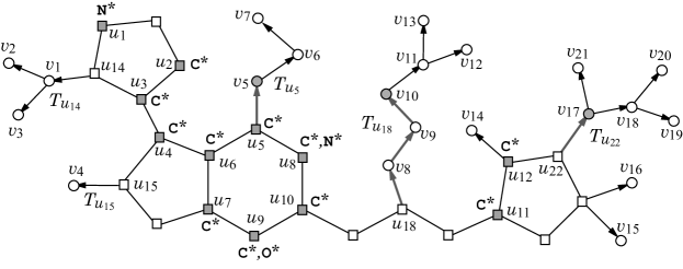
Figure 8: An illustration of a $(\sigma_{\mathrm{co}},\sigma_{\mathrm{nc}})$-extension $H$ with $\mathrm{Cr}(H)=C$ with $n(H)=43$, $\mathrm{ch}(H)=5$ and $\mathrm{bl}_{2}(H)=3$, where the non-core-vertices are depicted with circles, the leaf 2-branches are depicted with gray circles, the 2-internal edges are depicted with thick gray arrows and the elements in $\Lambda^{*}(v)$, $v\in V_{\mathrm{C}}$ are indicated with asterisk.

4.4 Chemical Specification

A chemical specification $\sigma_{\mathrm{\alpha\beta}}$ consists of the following:

1. We choose a set $\Lambda$ of chemical elements

   $$\Lambda^{\mathrm{co}},\Lambda^{\mathrm{nc}}\subseteq\Lambda.$$

   For a chemical graph $G$, let $\mathrm{na}_{\tt a}(G)$ (resp., $\mathrm{na}_{\tt a}^{\mathrm{co}}(G)$ and $\mathrm{na}_{\tt a}^{\mathrm{nc}}(G)$) denote the number of vertices (resp., core-vertices and non-core-vertices) in $G$ assigned chemical element ${\tt a}\in\Lambda$ (resp., ${\tt a}\in\Lambda^{\mathrm{co}}$ and ${\tt a}\in\Lambda^{\mathrm{nc}}$).

2. We choose sets of symbols

   $$\Lambda_{\mathrm{dg}}^{\mathrm{co}}\subseteq\Lambda_{\mathrm{dg}}(\Lambda^{\mathrm{co}},\mathrm{val}),~{}~{}~{}\Lambda_{\mathrm{dg}}^{\mathrm{nc}}\subseteq\Lambda_{\mathrm{dg}}(\Lambda^{\mathrm{nc}},\mathrm{val})$$

   such that $i\geq 2$ for any symbol ${\tt a}i\not\in\Lambda_{\mathrm{dg}}^{\mathrm{co}}$. the number of core-vertices $v$ with $\alpha(v)={\tt a}$ and $\deg_{G}(v)=i$ for $\mu={\tt a}i$. We choose sets of edge-configurations

   $$\Gamma^{\mathrm{co}}\subseteq\Gamma_{<}(\Lambda_{\mathrm{dg}}^{\mathrm{co}})\cup\Gamma_{=}(\Lambda_{\mathrm{dg}}^{\mathrm{co}}),~{}~{}\Gamma^{\mathrm{nc}}\subseteq\Gamma(\Lambda_{\mathrm{dg}}^{\mathrm{nc}}),$$

   $$\Gamma^{\mathrm{in}}\subseteq\Gamma^{\mathrm{nc}},~{}~{}~{}\Gamma^{\mathrm{ex}}\subseteq\Gamma^{\mathrm{nc}}$$

   such that $i,j\geq 2$ for any tuple $({\tt a}i,{\tt b}j,m)\not\in\Gamma^{\mathrm{in}}$.
   Define $\Gamma^{\mathrm{co}}_{>}\triangleq\{\overline{\gamma}=(\xi,\mu,m)\mid\gamma=(\mu,\xi,m)\in\Gamma^{\mathrm{co}},\mu<\xi\}$.

3. The induced adjacency-configuration $\mathrm{ac}(\gamma)$ of an edge-configuration $({\tt a}d,{\tt b}d^{\prime},m)$ is defined to be the adjacency-configuration $\mathrm{ac}(\gamma)=({\tt a},{\tt b},m)$. Set the following sets of adjacency-configurations:

   $$\Gamma_{\mathrm{ac}}^{\mathrm{co}}:=\{\mathrm{ac}(\gamma)\mid\gamma\in\Gamma^{\mathrm{co}}\},\Gamma_{\mathrm{ac,>}}^{\mathrm{co}}:=\{\mathrm{ac}(\gamma)\mid\gamma\in\Gamma^{\mathrm{co}}_{>}\},$$

   $$\Gamma_{\mathrm{ac}}^{\mathrm{in}}:=\{\mathrm{ac}(\gamma)\mid\gamma\in\Gamma^{\mathrm{in}}\},\Gamma_{\mathrm{ac}}^{\mathrm{ex}}:=\{\mathrm{ac}(\gamma)\mid\gamma\in\Gamma^{\mathrm{ex}}\}.$$

   In a chemical specification, we define the adjacency-configuration of a core-edge $uv$ to be $({\tt a},{\tt b},\beta(uv))$ with $\{{\tt a},{\tt b}\}=\{\alpha(u),\alpha(v)\}$ and the adjacency-configuration of a directed non-core edge $(u,v)$ to be $(\alpha(u),\alpha(v),\beta(uv))$.
   Let $\mathrm{ac}_{\nu}^{\mathrm{co}}(G)$ (resp., $\mathrm{ac}_{\nu}^{\mathrm{in}}(G)$ and $\mathrm{ac}_{\nu}^{\mathrm{ex}}(G)$) denote the number of core-edges (resp., directed ${\rho}$-internal edges and directed ${\rho}$-external edges) in $G$ assigned adjacency-configuration $\nu\in\Gamma_{\mathrm{ac}}^{\mathrm{co}}$ (resp., $\nu\in\Gamma_{\mathrm{ac}}^{\mathrm{in}}$ and $\nu\in\Gamma_{\mathrm{ac}}^{\mathrm{ex}}$).

4. Subsets $\Lambda^{*}(v)$, $v\in V_{\mathrm{C}}$ of elements that are allowed to be assigned to vertex $v\in V_{\mathrm{C}}$;

5. Lower and upper bound functions $\mathrm{na}_{\mathrm{LB}},\mathrm{na}_{\mathrm{UB}}:\Lambda\to[1,n^{*}]$ and $\mathrm{na}_{\mathrm{LB}}^{\mathrm{t}},\mathrm{na}_{\mathrm{UB}}^{\mathrm{t}}:\Lambda^{\mathrm{t}}\to[1,n^{*}]$, $\mathrm{t}\in\{\mathrm{co},\mathrm{nc}\}$ on the number of core-vertices and non-core-vertices, respectively, assigned chemical element ${\tt a}$.

6. Lower and upper bound functions $\mathrm{ns}_{\mathrm{LB}},\mathrm{ns}_{\mathrm{UB}}:\Lambda_{\mathrm{dg}}\to[1,n^{*}]$ and $\mathrm{ns}_{\mathrm{LB}}^{\mathrm{t}},\mathrm{ns}_{\mathrm{UB}}^{\mathrm{t}}:\Lambda_{\mathrm{dg}}^{\mathrm{t}}\to[1,n^{*}]$, $\mathrm{t}\in\{\mathrm{co},\mathrm{nc}\}$ on the number of core-vertices and non-core-vertices, respectively, assigned symbol $\mu$.

7. Lower and upper bound functions $\mathrm{ac}_{\mathrm{LB}}^{\mathrm{t}},\mathrm{ac}_{\mathrm{UB}}^{\mathrm{t}}:\Gamma_{\mathrm{ac}}^{\mathrm{t}}\to\mathbb{Z}_{+}$, $\mathrm{t}\in\{\mathrm{co},\mathrm{in},\mathrm{ex}\}$ on the number of core-edges, directed ${\rho}$-internal edges and directed ${\rho}$-external edges, respectively, assigned adjacency-configuration $\nu$.

8. Lower and upper bound functions $\mathrm{ec}_{\mathrm{LB}}^{\mathrm{t}},\mathrm{ec}_{\mathrm{UB}}^{\mathrm{t}}:\Gamma^{\mathrm{t}}\to\mathbb{Z}_{+}$, $\mathrm{t}\in\{\mathrm{co},\mathrm{in},\mathrm{ex}\}$ on the number of core-edges, directed ${\rho}$-internal edges and directed ${\rho}$-external edges, respectively, assigned edge-configurations $\gamma$.

9. Lower and upper functions $\mathrm{bd}_{m,\mathrm{LB}},\mathrm{bd}_{m,\mathrm{UB}}:E_{\mathrm{C}}\to\mathbb{Z}_{+}$, $m\in[2,3]$, where $\mathrm{bd}_{2,\mathrm{LB}}(e)+\mathrm{bd}_{3,\mathrm{LB}}(e)\leq\ell_{\mathrm{UB}}(e)$, $e\in E_{\mathrm{C}}$;

10. Side constraints: Lower and upper bounds on the number of some adjacency-configurations and edge-configurations; We can specify additional linear constraints on $\ell(P_{i})$, $\mathrm{bl}(P_{i})$ and the number $\mathrm{na}_{\tt a}(P_{i})$ of chemical element ${\tt a}$ in the path $P_{i}$, $a_{i}\in E_{\mathrm{C}}$ such as $\mathrm{na}_{\tt N}(P_{2})+\mathrm{na}_{\tt N}(P_{3})\leq c$ for a constant $c$ and nitrogen ${\tt N}\in\Lambda$.

An example of a chemical specification $\sigma_{\mathrm{\alpha\beta}}$ to the seed graph $G_{\mathrm{C}}$ in Figure 6 is given in Table 3.

For a graph $H\in\mathcal{H}(G_{\mathrm{C}},\sigma_{\mathrm{co}},\sigma_{\mathrm{nc}})$, let $\alpha:V(H)\to\Lambda$ and $\beta:E(H)\to[1,3]$ be functions. Then $G=(H,\alpha,\beta)$ is called a $(\sigma_{\mathrm{co}},\sigma_{\mathrm{nc}},\sigma_{\mathrm{\alpha\beta}})$-extension of $G_{\mathrm{C}}$ if the following hold:

1. $\sum_{uv\in E}\beta(uv)\leq\mathrm{val}(\alpha(u))$ for each vertex $u\in V(H)$; $\tau(e)\in\Gamma^{\mathrm{co}}$ for each core-edge $e$; $\tau(e)\in\Gamma^{\mathrm{in}}$ for each directed ${\rho}$-internal edge; and $\tau(e)\in\Gamma^{\mathrm{ex}}$ for each directed ${\rho}$-external edge.

2. $\alpha(v)\in\Lambda^{*}(v)$ for each vertex $v\in V_{\mathrm{C}}$.

3. It holds that $\mathrm{na}_{\tt a}(G)\in[\mathrm{na}_{\mathrm{LB}}({\tt a}),\mathrm{na}_{\mathrm{UB}}({\tt a})]$, ${\tt a}\in\Lambda$, $\mathrm{na}_{\tt a}^{\mathrm{co}}(G)\in[\mathrm{na}_{\mathrm{LB}}^{\mathrm{co}}({\tt a}),\mathrm{na}_{\mathrm{UB}}^{\mathrm{co}}({\tt a})]$, ${\tt a}\in\Lambda^{\mathrm{co}}$, and $\mathrm{na}_{\tt a}^{\mathrm{nc}}(G)\in[\mathrm{na}_{\mathrm{LB}}^{\mathrm{nc}}({\tt a}),\mathrm{na}_{\mathrm{UB}}^{\mathrm{nc}}({\tt a})]$, ${\tt a}\in\Lambda^{\mathrm{nc}}$;

4. It holds that $\mathrm{ns}_{\mu}(G)\in[\mathrm{na}_{\mathrm{LB}}(\mu),\mathrm{na}_{\mathrm{UB}}(\mu)]$, $\mu\in\Lambda_{\mathrm{dg}}$, $\mathrm{ns}_{\mu}^{\mathrm{co}}(G)\in[\mathrm{ns}_{\mathrm{LB}}^{\mathrm{co}}(\mu),\mathrm{ns}_{\mathrm{UB}}^{\mathrm{co}}(\mu)]$, $\mu\in\Lambda_{\mathrm{dg}}^{\mathrm{co}}$, and $\mathrm{ns}_{\mu}^{\mathrm{nc}}(G)\in[\mathrm{ns}_{\mathrm{LB}}^{\mathrm{nc}}(\mu),\mathrm{ns}_{\mathrm{UB}}^{\mathrm{nc}}(\mu)]$, $\mu\in\Lambda_{\mathrm{dg}}^{\mathrm{nc}}$;

5. It holds that $\mathrm{ac}_{\nu}^{\mathrm{co}}(G)\in[\mathrm{ac}_{\mathrm{LB}}^{\mathrm{co}}(\nu),\mathrm{ac}_{\mathrm{UB}}^{\mathrm{co}}(\nu)]$, $\nu\in\Gamma_{\mathrm{ac}}^{\mathrm{co}}$, $\mathrm{ac}_{\nu}^{\mathrm{in}}(G)\in[\mathrm{ac}_{\mathrm{LB}}^{\mathrm{in}}(\nu),\mathrm{ac}_{\mathrm{UB}}^{\mathrm{in}}(\nu)]$, $\nu\in\Gamma_{\mathrm{ac}}^{\mathrm{in}}$, and $\mathrm{ac}_{\nu}^{\mathrm{ex}}(G)\in[\mathrm{ac}_{\mathrm{LB}}^{\mathrm{ex}}(\nu),\mathrm{ac}_{\mathrm{UB}}^{\mathrm{ex}}(\nu)]$, $\nu\in\Gamma_{\mathrm{ac}}^{\mathrm{ex}}$;

6. It holds that $\mathrm{ec}_{\gamma}^{\mathrm{co}}(G)\in[\mathrm{ec}_{\mathrm{LB}}^{\mathrm{co}}(\gamma),\mathrm{ec}_{\mathrm{UB}}^{\mathrm{co}}(\gamma)]$, $\gamma\in\Gamma^{\mathrm{co}}$, $\mathrm{ec}_{\gamma}^{\mathrm{in}}(G)\in[\mathrm{ec}_{\mathrm{LB}}^{\mathrm{in}}(\gamma),\mathrm{ec}_{\mathrm{UB}}^{\mathrm{in}}(\gamma)]$, $\gamma\in\Gamma^{\mathrm{in}}$, and $\mathrm{ec}_{\gamma}^{\mathrm{ex}}(G)\in[\mathrm{ec}_{\mathrm{LB}}^{\mathrm{ex}}(\gamma),\mathrm{ec}_{\mathrm{UB}}^{\mathrm{ex}}(\gamma)]$, $\gamma\in\Gamma^{\mathrm{ex}}$;

7. For each edge $e\in E_{(\geq 2)}\cup E_{(\geq 1)}$, $|\{e\in E(P_{e})\mid\beta(e)=m\}|\in[\mathrm{bd}_{m,\mathrm{LB}}(e),\mathrm{bd}_{m,\mathrm{UB}}(e)]$;

8. The additional linear constraints are satisfied.

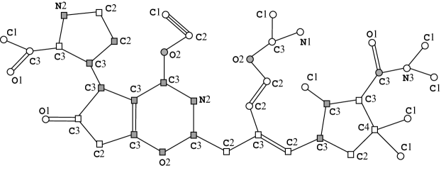
Figure 9: An illustration of a $(\sigma_{\mathrm{co}},\sigma_{\mathrm{nc}},\sigma_{\mathrm{\alpha\beta}})$-extension $G=(H,\alpha,\beta)$ of the seed graph $G_{\mathrm{C}}$ in Figure 6 with the specifications $\sigma_{\mathrm{co}},\sigma_{\mathrm{nc}}$ and $\sigma_{\mathrm{\alpha\beta}}$in Tables 1, 2 and 3, respectively, where a symbol $\mu\in\Lambda_{\mathrm{dg}}$ is depicted with a pair of an element ${\tt a}$ and a degree $i$ such as ${\tt C}1$.

Figure 9 illustrates one of the $(\sigma_{\mathrm{co}},\sigma_{\mathrm{nc}},\sigma_{\mathrm{\alpha\beta}})$-extensions of the seed graph $G_{\mathrm{C}}$ in Figure 6 with the specifications $\sigma_{\mathrm{co}},\sigma_{\mathrm{nc}}$ and $\sigma_{\mathrm{\alpha\beta}}$ in Tables 1, 2 and 3, respectively,

Let $\mathcal{G}(G_{\mathrm{C}},\sigma_{\mathrm{co}},\sigma_{\mathrm{nc}},\sigma_{\mathrm{\alpha\beta}})$ denote the set of all $(\sigma_{\mathrm{co}},\sigma_{\mathrm{nc}},\sigma_{\mathrm{\alpha\beta}})$-extensions of $G_{\mathrm{C}}$.

When a required condition on a target chemical graph to be inferred is described with a target specification $(\sigma_{\mathrm{co}},\sigma_{\mathrm{nc}},\sigma_{\mathrm{\alpha\beta}})$ with a seed graph $G_{\mathrm{C}}$, the inverse QSAR/QSPR can be formulated as an MILP, as discussed in the next section.

Table 3: Example 3 of a chemical specification $\sigma_{\mathrm{\alpha\beta}}$.

$\Lambda=\{{\tt C,N,O}\}$

$\Lambda_{\mathrm{dg}}^{\mathrm{co}}=\{{\tt C}2,{\tt C}3,{\tt C}4,{\tt N}2,{\tt O}2\}$

$\Lambda_{\mathrm{dg}}^{\mathrm{nc}}=\{{\tt C}1,{\tt C}2,{\tt C}3,{\tt C}4,{\tt N}1,{\tt N}3,{\tt O}1,{\tt O}2\}$

$\Gamma_{\mathrm{ac}}^{\mathrm{co}}$	$\nu_{1}^{\mathrm{co}}=({\tt C},{\tt C},1),\nu_{2}^{\mathrm{co}}=({\tt C},{\tt C},2),\nu_{3}^{\mathrm{co}}=({\tt C},{\tt N},1),\nu_{4}^{\mathrm{co}}=({\tt C},{\tt O},1)$
$\Gamma_{\mathrm{ac,>}}^{\mathrm{co}}$	$\overline{\nu_{3}}^{\mathrm{co}}=({\tt N},{\tt C},1),\overline{\nu_{4}}^{\mathrm{co}}=({\tt O},{\tt C},1)$
$\Gamma_{\mathrm{ac}}^{\mathrm{in}}$	$\nu_{1}^{\mathrm{in}}=({\tt C},{\tt C},1),\nu_{2}^{\mathrm{in}}=({\tt C},{\tt C},2),\nu_{3}^{\mathrm{in}}=({\tt C},{\tt O},1)$
$\Gamma_{\mathrm{ac}}^{\mathrm{ex}}$	$\nu_{1}^{\mathrm{ex}}=({\tt C},{\tt C},1),\nu_{2}^{\mathrm{ex}}=({\tt C},{\tt C},3),\nu_{3}^{\mathrm{ex}}=({\tt C},{\tt N},1),\nu_{4}^{\mathrm{ex}}=({\tt N},{\tt C},1),\nu_{5}^{\mathrm{ex}}=({\tt C},{\tt O},1),\nu_{6}^{\mathrm{ex}}=({\tt C},{\tt O},2),$
	$\nu_{7}^{\mathrm{ex}}=({\tt O},{\tt C},1)$

$\Gamma^{\mathrm{co}}$	$\gamma_{1}^{\mathrm{co}}=({\tt C}2,{\tt C}2,1),\gamma_{2}^{\mathrm{co}}=({\tt C}2,{\tt C}3,1),\gamma_{3}^{\mathrm{co}}=({\tt C}2,{\tt C}3,2),\gamma_{4}^{\mathrm{co}}=({\tt C}2,{\tt C}4,1),\gamma_{5}^{\mathrm{co}}=({\tt C}3,{\tt C}3,1),$
	$\gamma_{6}^{\mathrm{co}}=({\tt C}3,{\tt C}3,2),\gamma_{7}^{\mathrm{co}}=({\tt C}3,{\tt C}4,1),\gamma_{8}^{\mathrm{co}}=({\tt C}2,{\tt N}2,1),\gamma_{9}^{\mathrm{co}}=({\tt C}3,{\tt N}2,1),\gamma_{10}^{\mathrm{co}}=({\tt C}3,{\tt O}2,1)$
$\Gamma^{\mathrm{co}}_{>}$	$\overline{\gamma_{2}}^{\mathrm{co}}=({\tt C}3,{\tt C}2,1),\overline{\gamma_{3}}^{\mathrm{co}}=({\tt C}3,{\tt C}2,2),\overline{\gamma_{4}}^{\mathrm{co}}=({\tt C}4,{\tt C}2,1),\overline{\gamma_{7}}^{\mathrm{co}}=({\tt C}4,{\tt C}3,1),\overline{\gamma_{8}}^{\mathrm{co}}=({\tt N}2,{\tt C}2,1),$
	$\overline{\gamma_{9}}^{\mathrm{co}}=({\tt N}2,{\tt C}3,1),\overline{\gamma_{10}}^{\mathrm{co}}=({\tt O}2,{\tt C}3,1)$
$\Gamma^{\mathrm{in}}$	$\gamma_{1}^{\mathrm{in}}=({\tt C}2,{\tt C}2,2),\gamma_{2}^{\mathrm{in}}=({\tt C}3,{\tt C}2,1),\gamma_{3}^{\mathrm{in}}=({\tt C}3,{\tt C}3,1),\gamma_{4}^{\mathrm{in}}=({\tt C}2,{\tt O}2,1),\gamma_{5}^{\mathrm{in}}=({\tt C}3,{\tt O}2,1)$
$\Gamma^{\mathrm{ex}}$	$\gamma_{1}^{\mathrm{ex}}=({\tt C}3,{\tt C}1,1),\gamma_{2}^{\mathrm{ex}}=({\tt C}2,{\tt C}1,3),\gamma_{3}^{\mathrm{ex}}=({\tt C}3,{\tt C}3,1),\gamma_{4}^{\mathrm{ex}}=({\tt C}4,{\tt C}1,1),\gamma_{5}^{\mathrm{ex}}=({\tt C}3,{\tt N}1,1),$
	$\gamma_{6}^{\mathrm{ex}}=({\tt C}3,{\tt N}3,1),\gamma_{7}^{\mathrm{ex}}=({\tt C}3,{\tt O}1,2),\gamma_{8}^{\mathrm{ex}}=({\tt O}2,{\tt C}2,1),\gamma_{9}^{\mathrm{ex}}=({\tt O}2,{\tt C}3,1),\gamma_{10}^{\mathrm{ex}}=({\tt N}3,{\tt C}1,1)$

$\Lambda^{*}(u_{1})=\{{\tt N}\}$, $\Lambda^{*}(u_{8})=\{{\tt C,N}\}$, $\Lambda^{*}(u_{9})=\{{\tt C,O}\}$, $\Lambda^{*}(u)=\{{\tt C}\}$, $u\in V_{\mathrm{C}}\setminus\{u_{1},u_{8},u_{9}\}$

	${\tt C}$	${\tt N}$	${\tt O}$
$\mathrm{na}_{\mathrm{LB}}(\lambda)$	27	1	1
$\mathrm{na}_{\mathrm{UB}}(\lambda)$	37	4	8

	${\tt C}$	${\tt N}$	${\tt O}$
$\mathrm{na}_{\mathrm{LB}}^{\mathrm{co}}(\lambda)$	9	1	0
$\mathrm{na}_{\mathrm{UB}}^{\mathrm{co}}(\lambda)$	23	4	5

	${\tt C}$	${\tt N}$	${\tt O}$
$\mathrm{na}_{\mathrm{LB}}^{\mathrm{nc}}(\lambda)$	9	1	2
$\mathrm{na}_{\mathrm{UB}}^{\mathrm{nc}}(\lambda)$	18	3	8

	${\tt C}1$	${\tt C}2$	${\tt C}3$	${\tt C}4$	${\tt N}1$	${\tt N}2$	${\tt N}3$	${\tt O}1$	${\tt O}2$
$\mathrm{ns}_{\mathrm{LB}}(\mu)$	6	7	12	0	0	0	0	0	0
$\mathrm{ns}_{\mathrm{UB}}(\mu)$	10	11	18	2	2	2	2	5	5

	${\tt C}2$	${\tt C}3$	${\tt C}4$	${\tt N}2$	${\tt N}3$	${\tt O}2$
$\mathrm{ns}_{\mathrm{LB}}^{\mathrm{co}}(\mu)$	3	5	0	0	0	0
$\mathrm{ns}_{\mathrm{UB}}^{\mathrm{co}}(\mu)$	8	15	2	2	3	5

	${\tt C}1$	${\tt C}2$	${\tt C}3$	${\tt C}4$	${\tt N}1$	${\tt N}2$	${\tt N}3$	${\tt O}1$	${\tt O}2$
$\mathrm{ns}_{\mathrm{LB}}^{\mathrm{nc}}(\mu)$	6	1	1	0	0	0	0	0	0
$\mathrm{ns}_{\mathrm{UB}}^{\mathrm{nc}}(\mu)$	10	5	5	2	2	2	2	5	5

	$\nu_{1}^{\mathrm{co}}$	$\nu_{2}^{\mathrm{co}}$	$\nu_{3}^{\mathrm{co}}$	$\nu_{4}^{\mathrm{co}}$
$\mathrm{ac}_{\mathrm{LB}}^{\mathrm{co}}(\nu)$	0	0	0	0
$\mathrm{ac}_{\mathrm{UB}}^{\mathrm{co}}(\nu)$	30	10	10	10

	$\nu_{1}^{\mathrm{in}}$	$\nu_{2}^{\mathrm{in}}$	$\nu_{3}^{\mathrm{in}}$
$\mathrm{ac}_{\mathrm{LB}}^{\mathrm{in}}(\nu)$	0	0	0
$\mathrm{ac}_{\mathrm{UB}}^{\mathrm{in}}(\nu)$	5	5	5

	$\nu_{1}^{\mathrm{ex}}$	$\nu_{2}^{\mathrm{ex}}$	$\nu_{3}^{\mathrm{ex}}$	$\nu_{4}^{\mathrm{ex}}$	$\nu_{5}^{\mathrm{ex}}$	$\nu_{6}^{\mathrm{ex}}$	$\nu_{7}^{\mathrm{ex}}$
$\mathrm{ac}_{\mathrm{LB}}^{\mathrm{ex}}(\nu)$	0	0	0	0	0	0	0
$\mathrm{ac}_{\mathrm{UB}}^{\mathrm{ex}}(\nu)$	10	10	10	10	10	10	10

	$\gamma_{1}^{\mathrm{co}}$	$\gamma_{2}^{\mathrm{co}}$	$\gamma_{3}^{\mathrm{co}}$	$\gamma_{4}^{\mathrm{co}}$	$\gamma_{5}^{\mathrm{co}}$	$\gamma_{6}^{\mathrm{co}}$	$\gamma_{7}^{\mathrm{co}}$	$\gamma_{8}^{\mathrm{co}}$	$\gamma_{9}^{\mathrm{co}}$	$\gamma_{10}^{\mathrm{co}}$
$\mathrm{ec}_{\mathrm{LB}}^{\mathrm{co}}(\gamma)$	0	0	0	0	0	0	0	0	0	0
$\mathrm{ec}_{\mathrm{UB}}^{\mathrm{co}}(\gamma)$	4	15	4	4	10	5	4	4	6	4

	$\gamma_{1}^{\mathrm{in}}$	$\gamma_{2}^{\mathrm{in}}$	$\gamma_{3}^{\mathrm{in}}$	$\gamma_{4}^{\mathrm{in}}$	$\gamma_{5}^{\mathrm{in}}$
$\mathrm{ec}_{\mathrm{LB}}^{\mathrm{in}}(\gamma)$	0	0	0	0	0
$\mathrm{ec}_{\mathrm{UB}}^{\mathrm{in}}(\gamma)$	3	3	3	3	3

	$\gamma_{1}^{\mathrm{ex}}$	$\gamma_{2}^{\mathrm{ex}}$	$\gamma_{3}^{\mathrm{ex}}$	$\gamma_{4}^{\mathrm{ex}}$	$\gamma_{5}^{\mathrm{ex}}$	$\gamma_{6}^{\mathrm{ex}}$	$\gamma_{7}^{\mathrm{ex}}$	$\gamma_{8}^{\mathrm{ex}}$	$\gamma_{9}^{\mathrm{ex}}$	$\gamma_{10}^{\mathrm{ex}}$
$\mathrm{ec}_{\mathrm{LB}}^{\mathrm{ex}}(\gamma)$	0	0	0	0	0	0	0	0	0	0
$\mathrm{ec}_{\mathrm{UB}}^{\mathrm{ex}}(\gamma)$	8	4	4	4	4	4	6	4	4	4

	$a_{1}$	$a_{2}$	$a_{3}$	$a_{4}$	$a_{5}$	$a_{6}$	$a_{7}$	$a_{8}$	$a_{9}$	$a_{10}$	$a_{11}$	$a_{12}$	$a_{13}$	$a_{14}$	$a_{15}$	$a_{16}$
$\mathrm{bd}_{2,\mathrm{LB}}(a_{i})$	0	0	0	1	0	0	0	0	0	0	0	1	0	0	0	0
$\mathrm{bd}_{2,\mathrm{UB}}(a_{i})$	1	1	0	2	2	0	0	0	0	0	0	1	0	0	0	0

	$a_{1}$	$a_{2}$	$a_{3}$	$a_{4}$	$a_{5}$	$a_{6}$	$a_{7}$	$a_{8}$	$a_{9}$	$a_{10}$	$a_{11}$	$a_{12}$	$a_{13}$	$a_{14}$	$a_{15}$	$a_{16}$
$\mathrm{bd}_{3,\mathrm{LB}}(a_{i})$	0	0	0	0	0	0	0	0	0	0	0	0	0	0	0	0
$\mathrm{bd}_{3,\mathrm{UB}}(a_{i})$	0	0	0	0	1	0	0	0	0	0	0	0	0	0	0	0

4.5 Abstract Specification for Cores

The framework for the inverse QSAR/QSPR  [6, 11, 30] has been applied to a case of chemical graphs with an abstract topological structure such as acyclic or monocyclic graphs by Ito et al. [3] and rank-2 cyclic graphs with a specified polymer topology with a cycle index up to 2 by Zhu et al. [30].

We show that such classes of cyclic graphs can be specified with part of our target specification $(\sigma_{\mathrm{co}},\sigma_{\mathrm{nc}},\sigma_{\mathrm{\alpha\beta}})$ to a seed graph.

In their applications [11, 30], a set $\Lambda$ of chemical elements is given and the graph size $n(G)$, the core size $\mathrm{cs}(G)$ and the core height $\mathrm{ch}(G)$ of a target graph $G$ are required to be prescribed values $\mathrm{cs}^{\dagger}$, $\mathrm{ch}^{\dagger}$ and $n^{\dagger}$. Then we specify the bounds on these values in $\sigma_{\mathrm{nc}}$ so that $n_{\mathrm{LB}}:=n^{*}:=n^{\dagger}$; $\mathrm{cs}_{\mathrm{LB}}:=\mathrm{cs}_{\mathrm{UB}}:=\mathrm{cs}^{\dagger}$; $\mathrm{ch}_{\mathrm{LB}}(\mathrm{t}):=\mathrm{ch}_{\mathrm{UB}}(\mathrm{t}):=\mathrm{ch}^{\dagger}$ for some graph element $\mathrm{t}\in V_{\mathrm{C}}\cup E_{(\geq 2)}\cup E_{(\geq 1)}$; and $\mathrm{ch}_{\mathrm{LB}}(\mathrm{t}):=0$, $\mathrm{ch}_{\mathrm{UB}}(\mathrm{t}):=\mathrm{ch}^{\dagger}$ for the other elements $\mathrm{t}\in V_{\mathrm{C}}\cup E_{(\geq 2)}\cup E_{(\geq 1)}$. We set $\Lambda_{\mathrm{dg}}^{\mathrm{co}}$ and $\Lambda_{\mathrm{dg}}^{\mathrm{nc}}$ to be the sets of all possible symbols in $\Lambda\times[1,4]$ and set $\Gamma^{\mathrm{co}}$, $\Gamma^{\mathrm{in}}$ and $\Gamma^{\mathrm{ex}}$ to be the sets of all possible edge-configurations in $\sigma_{\mathrm{\alpha\beta}}$.

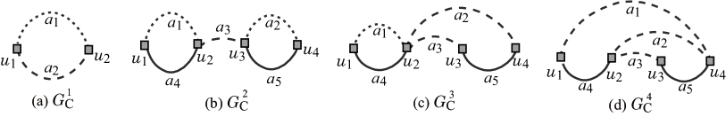
Figure 10: An illustration of seed graphs for inferring cyclic graphs with rank at most 2: (a) A seed graph $G_{\mathrm{C}}^{1}$ for monocyclic graphs; (b) A seed graph $G_{\mathrm{C}}^{2}$ for rank-2 cyclic graphs with the polymer topology $M_{1}\in\mathcal{PT}(2,4)$ in Figure 3(d); (c) A seed graph $G_{\mathrm{C}}^{3}$ for rank-2 cyclic graphs with the polymer topology $M_{2}\in\mathcal{PT}(2,4)$ in Figure 3(e); (d) A seed graph $G_{\mathrm{C}}^{4}$ for rank-2 cyclic graphs with the polymer topology $M_{3}\in\mathcal{PT}(2,4)$ in Figure 3(f).

A seed graph for inferring a chemical monocyclic graphs can be selected as a multigraph $G_{\mathrm{C}}^{1}$ with a vertex set $V_{\mathrm{C}}=\{u_{1},u_{2}\}$ and edge sets $E_{(\geq 2)}=\{a_{1}\}$ and $E_{(\geq 1)}=\{a_{2}\}$, as illustrated in Figure 10(a). We can include a linear constraint $\ell(a_{1})\leq\ell(a_{2})$ as part of the side constraint in $\sigma_{\mathrm{co}}$. This constraints reduces the search space on an MILP.

A seed graph for inferring a chemical rank-2 cyclic graphs with the polymer topology $M_{1}\in\mathcal{PT}(2,4)$ in Figure 3(d) can be selected as a multigraph $G_{\mathrm{C}}^{2}$ with a vertex set $V_{\mathrm{C}}=\{u_{1},u_{2},u_{3},u_{4}\}$ and edge sets $E_{(\geq 2)}=\{a_{1},a_{2}\}$, $E_{(\geq 1)}=\{a_{3}\}$ and $E_{(=1)}=\{a_{4},a_{5}\}$, as illustrated in Figure 10(b). We can include a linear constraint $\ell(a_{1})\leq\ell(a_{2})$ as part of the side constraint in $\sigma_{\mathrm{co}}$.

A seed graph for inferring a chemical rank-2 cyclic graphs with the polymer topology $M_{2}\in\mathcal{PT}(2,4)$ in Figure 3(e) can be selected as a multigraph $G_{\mathrm{C}}^{3}$ with a vertex set $V_{\mathrm{C}}=\{u_{1},u_{2},u_{3},u_{4}\}$ and edge sets $E_{(\geq 2)}=\{a_{1}\}$, $E_{(\geq 1)}=\{a_{2},a_{3}\}$ and $E_{(=1)}=\{a_{4},a_{5}\}$, as illustrated in Figure 10(c). We can include a linear constraint $\ell(a_{1})\leq\ell(a_{2})+\ell(a_{3})$ and $\ell(a_{2})\leq\ell(a_{3})$ in $\sigma_{\mathrm{co}}$.

A seed graph for inferring a chemical rank-2 cyclic graphs with the polymer topology $M_{3}\in\mathcal{PT}(2,4)$ in Figure 3(f) can be selected as a multigraph $G_{\mathrm{C}}^{4}$ with a vertex set $V_{\mathrm{C}}=\{u_{1},u_{2},u_{3},u_{4}\}$ and edge sets $E_{(\geq 1)}=\{a_{1},a_{2},a_{3}\}$ and $E_{(=1)}=\{a_{4},a_{5}\}$, as illustrated in Figure 10(d). We can include a linear constraint $\ell(a_{2})\leq\ell(a_{1})+1$, $\ell(a_{2})\leq\ell(a_{3})+1$ and $\ell(a_{1})\leq\ell(a_{3})$ in $\sigma_{\mathrm{co}}$.

5 MILPs for Chemical ${\rho}$-lean Graphs

Let $(G_{\mathrm{C}},\sigma_{\mathrm{co}},\sigma_{\mathrm{nc}},\sigma_{\mathrm{\alpha\beta}})$ be a target specification, where ${\rho}$ denotes the branch-parameter in $\sigma_{\mathrm{nc}}$. In this section, we formulate to an MILP $\mathcal{M}(x,g;\mathcal{C}_{2})$ in Stage 4 for inferring a chemical ${\rho}$-lean cyclic graph $G\in\mathcal{G}(G_{\mathrm{C}},\sigma_{\mathrm{co}},\sigma_{\mathrm{nc}},\sigma_{\mathrm{\alpha\beta}})$.

5.1 Scheme Graphs

Recall that we treat the underlying graph of a chemical cyclic graph as a mixed graph to define our descriptors, where core-edges are undirected edges and non-core-edges are directed. To formulate an MILP that infers a chemical cyclic graph, we further assign a direction of each core-edge so that constraints on a function $\tau:E\to\Gamma$ can be described notationally simpler.

Our method first gives directions to the edges in a given seed graph such that $V_{\mathrm{C}}=\{u_{1},u_{2},\ldots,u_{p}\}$, $E_{\mathrm{C}}=\{a_{1},a_{2},\ldots,a_{q}\}$ and each edge $a_{i}\in E_{\mathrm{C}}$ is a directed edge $a_{i}=(u_{j},u_{h})$ with $j<h$. Let $\widetilde{V_{\mathrm{C}}}$ denote the set of vertices $u\in V_{\mathrm{C}}$ such that $\mathrm{bl}_{\mathrm{UB}}(u)=1$ and $\widetilde{{t_{\mathrm{C}}}}=|\widetilde{V_{\mathrm{C}}}|$. Our method first arranges the order of verices in $V_{\mathrm{C}}$ so that

$$\mathrm{bl}_{\mathrm{UB}}(u_{i})=1 i\in[1,\widetilde{{t_{\mathrm{C}}}}] \mathrm{bl}_{\mathrm{UB}}(u_{i})=0 i\in[\widetilde{{t_{\mathrm{C}}}}+1,{t_{\mathrm{C}}}]$$, and , .

Next our method adds some more vertices and edges to the resulting digraph $G_{\mathrm{C}}$ to construct a digraph, called a scheme graph $\mathrm{SG}=(\mathcal{V},\mathcal{E})$ so that any ${\rho}$-lean graph $H\in\mathcal{H}(G_{\mathrm{C}},\sigma_{\mathrm{co}},\sigma_{\mathrm{nc}})$ (i.e., any $(\sigma_{\mathrm{co}},\sigma_{\mathrm{nc}})$-extension $H$ of $G_{\mathrm{C}}$) can be chosen as a subgraph of the scheme graph $\mathrm{SG}$.

To construct a scheme graph, our method first computes some integers that determine the size of each building block in $\mathrm{SG}$.

For a given specification $(\sigma_{\mathrm{co}},\sigma_{\mathrm{nc}})$, define

$$\begin{array}[]{ll}\displaystyle{\widetilde{\mathrm{ch}}_{\mathrm{LB}}\triangleq\sum_{v\in V_{\mathrm{C}}}\mathrm{ch}_{\mathrm{LB}}(v)+\sum_{e\in E_{(\geq 1)}\cup E_{(\geq 2)}}\mathrm{ch}_{\mathrm{LB}}(e)}&\\ \displaystyle{\mathrm{bl}^{*}_{\mathrm{LB}}\triangleq\sum_{v\in V_{\mathrm{C}}}\mathrm{bl}_{\mathrm{LB}}(v)+\sum_{e\in E_{(\geq 1)}\cup E_{(\geq 2)}}\mathrm{bl}_{\mathrm{LB}}(e),}&\displaystyle{\mathrm{bl}^{*}_{\mathrm{UB}}\triangleq\sum_{v\in V_{\mathrm{C}}}\mathrm{bl}_{\mathrm{UB}}(v)+\sum_{e\in E_{(\geq 1)}\cup E_{(\geq 2)}}\mathrm{bl}_{\mathrm{UB}}(e),}\end{array}$$

$${\ell^{*}_{\mathrm{inl}}\triangleq\sum_{v\in V_{\mathrm{C}}}\max\{\mathrm{ch}_{\mathrm{UB}}(v)-{\rho},0\}+\sum_{e\in E_{(\geq 1)}\cup E_{(\geq 2)}}\mathrm{bl}_{\mathrm{UB}}(e)\cdot\max\{\mathrm{ch}_{\mathrm{UB}}(e)-{\rho},0\},}$$

$$\beta^{*}_{i}\triangleq|E_{(\geq 2)}(u_{i})|+|E_{(\geq 1)}(u_{i})|+\sum_{e\in E_{(=1)}(u_{i})}(1+\mathrm{bd}_{2,\mathrm{LB}}(e)+2\mathrm{bd}_{3,\mathrm{LB}}(e))+\mathrm{bl}_{\mathrm{LB}}(u_{i}),~{}u_{i}\in V_{\mathrm{C}},$$

$$\Delta_{i}:=4-\beta^{*}_{i},~{}u_{i}\in V_{\mathrm{C}}.$$

Define integers that determine the size of a scheme graph $\mathrm{SG}$ as follows.

$$\begin{array}[]{l}{t_{\mathrm{C}}}:=|V_{\mathrm{C}}|,\widetilde{{t_{\mathrm{C}}}}:=|\{u\in V_{\mathrm{C}}\mid\mathrm{bl}_{\mathrm{UB}}(u)=1\}|,m_{\mathrm{C}}:=|E_{\mathrm{C}}|,\\ {t_{\mathrm{T}}}:=\mathrm{cs}_{\mathrm{UB}}-|V_{\mathrm{C}}|,\\ {t_{\mathrm{F}}}:=\min\bigl{[}n^{*}-\mathrm{cs}_{\mathrm{LB}}-\max\{\widetilde{\mathrm{ch}}_{\mathrm{LB}},{\rho}\cdot\mathrm{bl}^{*}_{\mathrm{LB}}\},\ell^{*}_{\mathrm{inl}}\bigr{]},\\ \mbox{$d_{\max}:=3$ if $\mathrm{dg}^{\mathrm{nc}}_{4,\mathrm{UB}}=0$; $d_{\max}:=4$ if $\mathrm{dg}^{\mathrm{nc}}_{4,\mathrm{UB}}\geq 1$, }\\ n_{\mathrm{C}}(i):=\Delta_{i}\cdot((d_{\max}\!-\!1)^{{\rho}}-1)/(d_{\max}-2),\\ n_{\mathrm{T}}:=2((d_{\max}\!-\!1)^{{\rho}}-1)/(d_{\max}-2),\\ n_{\mathrm{F}}:=(d_{\max}\!-\!1)((d_{\max}\!-\!1)^{{\rho}}-1)/(d_{\max}-2),\\ \displaystyle{m_{\mathrm{UB}}^{\mathrm{co}}:=\min\{n^{*}+\mathrm{r}(G_{\mathrm{C}}),m_{\mathrm{C}}+\!\!\!\!\sum_{e\in E_{(\geq 2)}\cup E_{(\geq 1)}}\!\!\!\!\ell_{\mathrm{UB}}(e)\},}\\ \displaystyle{m_{\mathrm{UB}}^{\mathrm{nc}}:=\min\{n^{*},{t_{\mathrm{F}}}+\!\!\sum_{i\in[1,{t_{\mathrm{C}}}]}n_{\mathrm{C}}(i)+n_{\mathrm{T}}\cdot{t_{\mathrm{T}}}+n_{\mathrm{F}}\cdot{t_{\mathrm{F}}}-1\},}\\ m_{\mathrm{UB}}:=\min\{n^{*}+\mathrm{r}(G_{\mathrm{C}}),m_{\mathrm{UB}}^{\mathrm{co}}+m_{\mathrm{UB}}^{\mathrm{nc}}\},\end{array}$$ (2)

where $n_{\mathrm{C}}(i)$ is the number of “edges” in the rooted tree $T(\Delta_{i},d_{\max}-1,{\rho})$, $n_{\mathrm{T}}$ is the number of “edges” in the rooted tree $T(2,d_{\max}-1,{\rho})$ and $n_{\mathrm{F}}$ is the number of “edges” in the rooted tree $T(d_{\max}-1,d_{\max}-1,{\rho})$. Recall that any core-vertex is allowed to be of degree 4.

Figure 11: An illustration of the structure of a scheme graph $\mathrm{SG}$, where vertices depicted with squares represent core-vertices, vertices depicted with gray circles represent ${\rho}$-internal-vertices, and vertices depicted with white circles represent ${\rho}$-external-vertices: (a) A seed graph $G_{\mathrm{C}}=(V_{\mathrm{C}},E_{\mathrm{C}}=E_{(\geq 2)}\cup E_{(\geq 1)}\cup E_{(0/1)}\cup E_{(=1)})$; (b) A tree $C_{i}$, $i\in[1,{t_{\mathrm{C}}}]$ rooted at a core-vertex ${v^{\mathrm{C}}}_{i,0}\in V_{\mathrm{C}}$; (c) A path $P_{\mathrm{T}}=(V_{\mathrm{T}},E_{\mathrm{T}})$ of length ${t_{\mathrm{T}}}-1$; (d) A tree $T_{i}$, $i\in[1,{t_{\mathrm{T}}}]$ rooted at a core-vertex ${v^{\mathrm{T}}}_{i,0}\in V_{\mathrm{T}}$; (e) A path $P_{\mathrm{F}}=(V_{\mathrm{F}},E_{\mathrm{F}})$ of length ${t_{\mathrm{F}}}-1$; (f) A rooted tree $F_{i}$, $i\in[1,{t_{\mathrm{F}}}]$ rooted at a ${\rho}$-internal vertex ${v^{\mathrm{F}}}_{i,0}\in V_{\mathrm{F}}$.

Formally the scheme graph $\mathrm{SG}=(\mathcal{V},\mathcal{E})$ is defined with a vertex set $\mathcal{V}=V_{\mathrm{C}}\cup V_{\mathrm{T}}\cup V_{\mathrm{F}}\cup V_{\mathrm{C}}^{\mathrm{ex}}\cup V_{\mathrm{T}}^{\mathrm{ex}}\cup V_{\mathrm{F}}^{\mathrm{ex}}$ and an edge set $\mathcal{E}=E_{\mathrm{C}}\cup E_{\mathrm{T}}\cup E_{\mathrm{F}}\cup E_{\mathrm{CT}}\cup E_{\mathrm{TC}}\cup E_{\mathrm{CF}}\cup E_{\mathrm{TF}}\cup E_{\mathrm{C}}^{\mathrm{ex}}\cup E_{\mathrm{T}}^{\mathrm{ex}}\cup E_{\mathrm{F}}^{\mathrm{ex}}$ that consist of the following sets.

Construction of the core $\mathrm{Cr}(H)$ of a $(\sigma_{\mathrm{co}},\sigma_{\mathrm{nc}})$-extension $H$ of $G_{\mathrm{C}}$: Denote the vertex set $V_{\mathrm{C}}$ and the edge set $E_{\mathrm{C}}$ in the seed graph $G_{\mathrm{C}}$ by $V_{\mathrm{C}}=\{{v^{\mathrm{C}}}_{i,0}\mid i\in[1,{t_{\mathrm{C}}}]\}$ and $E_{\mathrm{C}}=\{a_{i}\mid i\in[1,m_{\mathrm{C}}]\}$, respectively, where $V_{\mathrm{C}}$ is always included in $\mathrm{Cr}(H)$. For including additional core-vertices in $\mathrm{Cr}(H)$, introduce a path $P_{\mathrm{T}}=(V_{\mathrm{T}}=\{{v^{\mathrm{T}}}_{1,0},{v^{\mathrm{T}}}_{2,0},\ldots,$ ${v^{\mathrm{T}}}_{{t_{\mathrm{T}}},0}\},E_{\mathrm{T}}=\{{e^{\mathrm{T}}}_{1},{e^{\mathrm{T}}}_{2},\ldots,{e^{\mathrm{T}}}_{{t_{\mathrm{T}}}}\})$ of length ${t_{\mathrm{T}}}-1$ and a set $E_{\mathrm{CT}}$ (resp., $E_{\mathrm{TC}}$) of directed edges ${e^{\mathrm{CT}}}_{i,j}=({v^{\mathrm{C}}}_{i,0},{v^{\mathrm{T}}}_{j,0})$ (resp., ${e^{\mathrm{TC}}}_{i,j}=({v^{\mathrm{T}}}_{j,0},{v^{\mathrm{C}}}_{i,0})$) $i\in[1,{t_{\mathrm{C}}}]$, $j\in[1,{t_{\mathrm{T}}}]$. In $\mathrm{Cr}(H)$, an edge $a_{k}=({v^{\mathrm{C}}}_{i,0},{v^{\mathrm{C}}}_{i^{\prime},0})\in E_{(\geq 2)}\cup E_{(\geq 1)}$ is allowed to be replaced with a path $P_{k}$ from core-vertex ${v^{\mathrm{C}}}_{i,0}$ to core-vertex ${v^{\mathrm{C}}}_{i^{\prime},0}$ that visits a set of consecutive vertices ${v^{\mathrm{T}}}_{j,0},{v^{\mathrm{T}}}_{j+1,0},\ldots,{v^{\mathrm{T}}}_{j+p,0}\in V_{\mathrm{T}}$ and edge ${e^{\mathrm{TC}}}_{i,j}=({v^{\mathrm{C}}}_{i,0},{v^{\mathrm{T}}}_{j,0})\in E_{\mathrm{CT}}$, then edges ${e^{\mathrm{T}}}_{j+1},{e^{\mathrm{T}}}_{j+2},\ldots,{e^{\mathrm{T}}}_{j+p}\in E_{\mathrm{T}}$ and finally edge ${e^{\mathrm{TC}}}_{i^{\prime},j+p}=({v^{\mathrm{T}}}_{j+p,0},{v^{\mathrm{C}}}_{i^{\prime},0})\in E_{\mathrm{TC}}$. The vertices in $V_{\mathrm{T}}$ in the path will be core-vertices in $\mathrm{Cr}(H)$.

Construction of paths with ${\rho}$-internal edges in a $(\sigma_{\mathrm{co}},\sigma_{\mathrm{nc}})$-extension $H$ of $G_{\mathrm{C}}$: Introduce a path $P_{\mathrm{F}}=(V_{\mathrm{F}}=\{{v^{\mathrm{F}}}_{1,0},{v^{\mathrm{F}}}_{2,0},\ldots,$ ${v^{\mathrm{F}}}_{{t_{\mathrm{F}}},0}\},$ $E_{\mathrm{F}}=\{{e^{\mathrm{F}}}_{1},{e^{\mathrm{F}}}_{2},\ldots,{e^{\mathrm{F}}}_{{t_{\mathrm{F}}}}\})$ of length ${t_{\mathrm{F}}}-1$, a set $E_{\mathrm{CF}}$ of directed edges ${e^{\mathrm{CF}}}_{i,j}=({v^{\mathrm{C}}}_{i,0},{v^{\mathrm{F}}}_{j,0})$, $i\in[1,{t_{\mathrm{C}}}]$, $j\in[1,{t_{\mathrm{F}}}]$, and a set $E_{\mathrm{TF}}$ of directed edges ${e^{\mathrm{TF}}}_{i,j}=({v^{\mathrm{T}}}_{i,0},{v^{\mathrm{F}}}_{j,0})$, $i\in[1,{t_{\mathrm{T}}}]$, $j\in[1,{t_{\mathrm{F}}}]$. In $H$, a path $P$ with ${\rho}$-internal edges that starts from a core-vertex ${v^{\mathrm{C}}}_{i,0}\in V_{\mathrm{C}}$ (resp., ${v^{\mathrm{T}}}_{i,0}\in V_{\mathrm{T}}$) visits a set of consecutive vertices ${v^{\mathrm{F}}}_{j,0},{v^{\mathrm{F}}}_{j+1,0},\ldots,{v^{\mathrm{F}}}_{j+p,0}\in V_{\mathrm{F}}$ and edge ${e^{\mathrm{CF}}}_{i,h}=({v^{\mathrm{C}}}_{i,0},{v^{\mathrm{F}}}_{j,0})\in E_{\mathrm{CF}}$ (resp., ${e^{\mathrm{TF}}}_{i,j}=({v^{\mathrm{T}}}_{i,0},{v^{\mathrm{F}}}_{j,0})\in E_{\mathrm{TF}}$) and edges ${e^{\mathrm{F}}}_{j+1},{e^{\mathrm{F}}}_{j+2},\ldots,{e^{\mathrm{F}}}_{j+p}\in E_{\mathrm{F}}$. In $H$, the edges and the vertices (except for ${v^{\mathrm{C}}}_{i,0}$) in the path $P$ are regarded as ${\rho}$-internal edges and ${\rho}$-internal vertices, respectively.

Construction of ${\rho}$-fringe-trees in a $(\sigma_{\mathrm{co}},\sigma_{\mathrm{nc}})$-extension $H$ of $G_{\mathrm{C}}$: In $H$, the root of a ${\rho}$-fringe-tree can be any vertex in $V_{\mathrm{C}}\cup V_{\mathrm{T}}\cup V_{\mathrm{F}}$. Let $\mathrm{X}\in\{\mathrm{C,T,F}\}$. Introduce a rooted tree $X_{i}$, $i\in[1,{t_{\mathrm{X}}}]$ at each vertex ${v^{\mathrm{X}}}_{i,0}$, where each $C_{i}$ is isomorphic to $T(d_{\max}-2,d_{\max}-1,{\rho})$, each $T_{i}$ is isomorphic to $T(2,d_{\max}-1,{\rho})$ and each $F_{i}$ is isomorphic to $T(d_{\max}-1,d_{\max}-1,{\rho})$. The $j$-th vertex (resp., edge) in each rooted tree $X_{i}$ is denoted by ${v^{\mathrm{X}}}_{i,j}$ (resp., ${e^{\mathrm{X}}}_{i,j}$) See Figure 11. Let $V_{\mathrm{X}}^{\mathrm{ex}}$ and $E_{\mathrm{X}}^{\mathrm{ex}}$ denote the set of non-root vertices ${v^{\mathrm{X}}}_{i,j}$ and the set of edges ${e^{\mathrm{X}}}_{i,j}$ over all rooted trees $X_{i}$, $i\in[1,{t_{\mathrm{X}}}]$. In $H$, a ${\rho}$-fringe-tree is selected as a subtree of $X_{i}$, $i\in[1,{t_{\mathrm{X}}}]$ with root ${v^{\mathrm{X}}}_{i,0}$.

We see that the scheme graph $\mathrm{SG}=(\mathcal{V},\mathcal{E})$ for a specification $(G_{\mathrm{C}},\sigma_{\mathrm{co}},\sigma_{\mathrm{nc}},\sigma_{\mathrm{\alpha\beta}})$ satisfies the following.

$$|\mathcal{V}|=O((n^{*}+\mathrm{cs}_{\mathrm{UB}})(d_{\max}-1)^{{\rho}}),~{}~{}~{}|\mathcal{E}|=O(|E_{\mathrm{C}}|+|\mathcal{V}|+n^{*}\cdot\mathrm{cs}_{\mathrm{UB}}).$$

5.2 Formulating an MILP for Choosing a Chemical Graph from a Scheme Graph

Let $K$ denote the dimension of a feature vector $x=f(G)$ used in constructing a prediction function $\psi$ over a set of chemical graphs $G$. Note that sets of chemical symbols and edge-configuration in Stages 4 and 5 can be subsets of those used in constructing a prediction function $\psi$ in Stage 3. Based on the above scheme graph $\mathrm{SG}$, we obtain an MILP formulation that satisfies the following result.

Theorem 2.

Let $(\sigma_{\mathrm{co}},\sigma_{\mathrm{nc}},\sigma_{\mathrm{\alpha\beta}})$ be a target specification and $|\Gamma|=|\Lambda_{\mathrm{dg}}^{\mathrm{co}}|+|\Lambda_{\mathrm{dg}}^{\mathrm{nc}}|+|\Gamma^{\mathrm{co}}|+|\Gamma^{\mathrm{in}}|+|\Gamma^{\mathrm{co}}|$ for sets of chemical symbols and edge-configuration in $\sigma_{\mathrm{\alpha\beta}}$. Then there is an MILP $\mathcal{M}(x,g;\mathcal{C}_{2})$ that consists of variable vectors $x\in\mathbb{R}^{K}$ and $g\in\mathbb{R}^{q}$ for an integer $q=O(\mathrm{cs}_{\mathrm{UB}}(|E_{\mathrm{C}}|+n^{*})+(|E_{\mathrm{C}}|+|\mathcal{V}|)|\Gamma|)$ and a set $\mathcal{C}_{2}$ of $O([\mathrm{cs}_{\mathrm{UB}}(|E_{\mathrm{C}}|+n^{*})+|\mathcal{V}|]|\Gamma|)$ constraints on $x$ and $g$ such that: $(x^{*},g^{*})$ is feasible to $\mathcal{M}(x,g;\mathcal{C}_{2})$ if and only if $g^{*}$ forms a chemical ${\rho}$-lean graph $G\in\mathcal{G}(G_{\mathrm{C}},\sigma_{\mathrm{co}},\sigma_{\mathrm{nc}},\sigma_{\mathrm{\alpha\beta}})$ such that $f(G)=x^{*}$.

Note that our MILP requires only $O(n^{*})$ variables and constraints when the branch-parameter ${\rho}$, integers $|E_{\mathrm{C}}|$, $\mathrm{cs}_{\mathrm{UB}}$ and $|\Gamma|$ are constant.

We explain the basic idea of our MILP in Theorem 2. The MILP mainly consists of the following three types of constraints.

1. Constraints for selecting a ${\rho}$-lean graph $H\in\mathcal{H}(G_{\mathrm{C}},\sigma_{\mathrm{co}},\sigma_{\mathrm{nc}})$ as a subgraph of the scheme graph $\mathrm{SG}$;

2. Constraints for assigning chemical elements to vertices and multiplicity to edges to determine a chemical graph $G=(H,\alpha,\beta)$; and

3. Constraints for computing descriptors from the selected chemical graph $G$.

In the constraints of C1, more formally we prepare the following.
Variables:
a binary variable ${v^{\mathrm{X}}}(i,j)\in\{0,1\}$ for each vertex ${v^{\mathrm{X}}}_{i,j}\in V_{\mathrm{X}}$, $\mathrm{X}\in\{\mathrm{C,T,F}\}$ so that ${v^{\mathrm{X}}}(i,j)=1$ $\Leftrightarrow$ vertex ${v^{\mathrm{X}}}_{i,j}$ is used in a graph $H$ selected from $\mathrm{SG}$;
a binary variable ${e^{\mathrm{X}}}(i)\in\{0,1\}$ (resp., ${e^{\mathrm{C}}}(i)\in\{0,1\}$) for each edge ${e^{\mathrm{X}}}_{i}\in E_{\mathrm{T}}\cup E_{\mathrm{F}}$ (resp., ${e^{\mathrm{C}}}_{i}=a_{i}\in E_{(\geq 2)}\cup E_{(\geq 1)}\cup E_{(0/1)}$) so that ${e^{\mathrm{X}}}(i)=1$ $\Leftrightarrow$ edge ${e^{\mathrm{X}}}_{i}$ is used in a graph $H$ selected from $\mathrm{SG}$. To save the number of variables in our MILP formulation, we do not prepare a binary variable ${e^{\mathrm{X}}}(i,j)\in\{0,1\}$ for any edge ${e^{\mathrm{X}}}_{i,j}\in E_{\mathrm{CT}}\cup E_{\mathrm{TC}}\cup E_{\mathrm{CF}}\cup E_{\mathrm{TC}}$, where we represent a choice of edges in these sets by a set of $O(n^{*}|E_{\mathrm{C}}|)$ variables (see [AN20] for the details);
Constraints:
linear constraints so that each ${\rho}$-fringe-tree of a graph $H$ from $\mathrm{SG}$ is selected a subtree of some of the rooted trees $C_{i}$, $i\in[1,{t_{\mathrm{C}}}]$, $T_{i}$, $i\in[1,{t_{\mathrm{T}}}]$ and $F_{i}$, $i\in[1,{t_{\mathrm{F}}}]$;
linear constraints such that each edge ${e^{\mathrm{C}}}_{i}=a_{i}\in E_{(=1)}$ is always used as a core-edge in $H$ and each edge ${e^{\mathrm{C}}}_{i}=a_{i}\in E_{(0/1)}$ is used as a core-edge in $H$ if necessary;
linear constraints such that for each edge $a_{k}=({v^{\mathrm{C}}}_{i},{v^{\mathrm{C}}}_{i^{\prime}})\in E_{(\geq 2)}$, vertex ${v^{\mathrm{C}}}_{i}\in V_{\mathrm{C}}$ is connected to vertex ${v^{\mathrm{C}}}_{i^{\prime}}\in V_{\mathrm{C}}$ in $H$ by a path $P_{k}$ that passes through some core-vertices in $V_{\mathrm{T}}$ and edges ${e^{\mathrm{CT}}}_{i,j},{e^{\mathrm{T}}}_{j+1},{e^{\mathrm{T}}}_{j+2},\ldots,{e^{\mathrm{T}}}_{j+p},{e^{\mathrm{TC}}}_{i^{\prime},j+p}$ for some integers $j$ and $p$;
linear constraints such that for each edge $a_{k}=({v^{\mathrm{C}}}_{i},{v^{\mathrm{C}}}_{i^{\prime}})\in E_{(\geq 1)}$, either the edge $a_{k}$ is used as a core-edge in $H$ or vertex ${v^{\mathrm{C}}}_{i}\in V_{\mathrm{C}}$ is connected to vertex ${v^{\mathrm{C}}}_{i^{\prime}}\in V_{\mathrm{C}}$ in $H$ by a path $P_{k}$ as in the case of edges in $E_{(\geq 2)}$;
linear constraints for selecting a path $P$ with ${\rho}$-internal edges ${e^{\mathrm{CF}}}_{i,j}$ (or ${e^{\mathrm{TF}}}_{i,j}$), ${e^{\mathrm{F}}}_{j+1},{e^{\mathrm{F}}}_{j+2},\ldots,{e^{\mathrm{F}}}_{j+p}$ for some integers $j$ and $p$.

Based on these, we include constraints with some more additional variables so that a selected subgraph $H$ is a connected graph and satisfies the core specification $\sigma_{\mathrm{co}}$ and the non-core specification $\sigma_{\mathrm{nc}}$. See constraints (4) to (10) in Appendix A.1 for choosing core-edges from the path $P_{\mathrm{T}}$. See constraints (11) to (18) in Appendix A.2 for choosing internal ${\rho}$-internal vertices/edges from the path $P_{\mathrm{F}}$. See constraints (19) to (32) in Appendix A.3 for choosing internal ${\rho}$-external vertices/edges from the trees $C_{i}$, $T_{i}$ and $F_{i}$.

In the constraints of C2, we prepare an integer variable ${\alpha}^{\mathrm{X}}(i,j)$ for each vertex ${v^{\mathrm{X}}}_{i,j}\in\mathcal{V}$, $\mathrm{X}\in\{\mathrm{C,T,F}\}$ in the scheme graph that represents the chemical element $\alpha({v^{\mathrm{X}}}_{i,j})\in\Lambda$ if ${v^{\mathrm{X}}}_{i,j}$ is in a selected graph $H$ (or $\alpha({v^{\mathrm{X}}}_{i,j})=0$ otherwise); integer variables $\beta^{\mathrm{C}}:E_{\mathrm{C}}\to[0,3]$, $\beta^{\mathrm{T}}:E_{\mathrm{T}}\to[0,3]$ and $\beta^{\mathrm{F}}:E_{\mathrm{F}}\to[0,3]$ that represent the bond-multiplicity of edges in $E_{\mathrm{C}}\cup E_{\mathrm{T}}\cup E_{\mathrm{F}}$; and integer variables $\beta^{+},\beta^{-}:E_{(\geq 2)}\cup E_{(\geq 1)}\to[0,3]$ and $\beta^{\mathrm{in}}:\widetilde{V_{\mathrm{C}}}\cup V_{\mathrm{T}}\to[0,3]$ that represent the bond-multiplicity of edges in $E_{\mathrm{CT}}\cup E_{\mathrm{TC}}\cup E_{\mathrm{CF}}\cup E_{\mathrm{TF}}$. This determines a chemical graph $G=(H,\alpha,\beta)$. Also we include constraints for a selected chemical graph $G$ to satisfy the valence condition at each vertex $v$ with the edge-configurations $\tau(e)$ of the edges incident to $v$ and the chemical specification $\sigma_{\mathrm{\alpha\beta}}$. See constraints (43) to (53) in Appendix A.5 for assigning multiplicity; and constraints (56) to (69) in Appendix A.6 for assigning chemical clements and satisfying valence condition.

In the constraints of C3, we introduce a variable for each descriptor and constraints with some more variables to compute the value of each descriptor in $f(G)$ for a selected chemical graph $G$. See constraints (33) to (42) in Appendix A.4 for descriptor of the number of specified degree; constraints (70) to (73) in Appendix A.7 for lower and upper bounds on the number of bonds in a chemical specification $\sigma_{\mathrm{\alpha\beta}}$; constraints (LABEL:eq:AC_first) to (84) in Appendix A.8 for descriptor of the number of adjacency-configurations; constraints (85) to (88) in Appendix A.9 for descriptor of the number of chemical symbols; and constraints (LABEL:eq:EC_first) to (99) in Appendix A.10 for descriptor of the number of edge-configurations. When we use adjacency-configuration in a feature vector $f(G)$ instead of edge-configuration, we do not need to include the constraints in Appendix A.10.

6 A New Graph Search Algorithm

This section designs a new algorithm for generating ${\rho}$-lean cyclic graphs $G$ that have the same feature vector $f(G^{\dagger})$ of a given chemical ${\rho}$-lean graph $G^{\dagger}$.

6.1 The New Aspects

We design a new algorithm for generating cyclic chemical graphs based on the following aspects:

1. Treat the non-core components of a cyclc graphs with a certain limited structure that frequently appears among chemical compounds registered in the chemical data base;

2. Instead of manipulating target graphs directly, first compute the frequency vectors $\boldsymbol{f}(G^{\prime})$ (some types of feature vectors) of subtrees $G^{\prime}$ of all target graphs and then construct a limited number of target graphs $G$ from the process of computing the vectors; and

3. First construct a chemical graph $G^{\dagger}\in\mathcal{G}$ with $\boldsymbol{f}(G^{\dagger})=x^{*}$ by solving an MILP in Stage 4 and restrict ourselves to a family of chemical graphs $G^{*}\in\mathcal{G}$ that have a common structure with the initial chemical graph $G^{\dagger}$.

In (a), we choose a small branch-parameter ${\rho}$ such as ${\rho}=2$ and treat chemical ${\rho}$-lean cyclic graphs $G$ such that each $2$-fringe-tree in $G$ satisfies the size constraint (1).

We design a method in (b) by extending the dynamic programming algorithm for generating acyclic chemical graphs proposed by Azam et al. [4]. The first phase of the algorithm computes some compressed forms of all substructures of target objects before the second phase realizes a final object based on the computation process of the first phase.

The idea of (c) is first introduced in this paper. Informally speaking, we first decompose the chemical graph $G^{\dagger}$ into a collection of chemical subtrees $T^{\dagger}_{1},T^{\dagger}_{2},\ldots,T^{\dagger}_{p}$ and then compute vectors $x^{*}_{1},x^{*}_{2},\ldots,x^{*}_{p}$ such that $\boldsymbol{f}(T^{\dagger}_{i})=x^{*}_{i}$, $i\in[1,p]$ and any collection of other chemical trees $T^{\dagger}_{i}$ with $\boldsymbol{f}(T^{\dagger}_{i})=x^{*}_{i}$ always gives rise to a target chemical graph $G^{*}\in G$. Thus this allows us to generate chemical trees $T^{\dagger}_{i}$ with $\boldsymbol{f}(T^{\dagger}_{i})=x^{*}_{i}$ for each index $i\in[1,p]$ independently before we combine them to get a chemical graph $G^{\dagger}\in G$ in Stage 5.

In the following, we describe a new algorithm that for a given ${\rho}$-lean chemical graph $G^{\dagger}=(H^{\dagger},\alpha^{\dagger},\beta^{\dagger})$, generates chemical ${\rho}$-lean cyclic graphs $G^{*}=(H,\alpha,\beta)$ such that

$$\boldsymbol{f}(G^{*})=\boldsymbol{f}(G^{\dagger}) \mathrm{Cr}(H) \mathrm{Cr}(H^{\dagger})$$ and the core is isomorphic to the core ,

where $G^{*}$ may not be isomorphic to $G^{\dagger}$ and the elements in $\Lambda$ may not correspond between the two cores; i.e., possibly $\alpha(v)\neq\alpha^{\dagger}(\phi(v))$ for some core-vertex $v$ of $H$ in the graph-isomorphism $\phi$ between $\mathrm{Cr}(H)$ and $\mathrm{Cr}(H^{\dagger})$.

In this section, we describe our new algorithm in a general setting where a branch-parameter is any integer ${\rho}\geq 1$ and a chemical graph $G$ to be inferred is any chemical ${\rho}$-lean cyclic graph.

6.2 Nc-trees and C-trees

Nc-trees Let ${\rho}$ be a branch-parameter. and $H$ be a ${\rho}$-lean cyclic graph. We have introduced core-subtrees in Section 2. We define “non-core-subtrees” as follows depending on branch-parameter ${\rho}$. Let $T$ be a connected subgraph of $H$. We call $T$ a non-core-subtree of $H$ if $T$ consists of a path $P_{\mathrm{in}}$ of a ${\rho}$-pendent-tree of $H$ and the ${\rho}$-fringe-trees rooted at vertices in $P_{\mathrm{in}}$. We call a non-core-subtree $T$ of $H$ an internal-subtree (resp., an end-subtree) of $H$ if neither (resp., one) of the two end-vertices of $P_{\mathrm{in}}$ is a leaf ${\rho}$-branch of $H$, as illustrated in Figure 12(a) (resp., in Figure 12(b)).

To represent a non-core-subtree of a ${\rho}$-lean cyclic graph $H$, we introduce “nc-trees.” We define an nc-tree to be a chemical bi-rooted tree $T$ such that each rooted tree $T^{\prime}\in\mathcal{F}(T)$ has a height at most ${\rho}$. For an nc-tree $T$, define
   $\widetilde{V}_{\mathrm{co}}(T)\triangleq\emptyset$ (resp., $\widetilde{E}_{\mathrm{co}}(T)\triangleq\emptyset$);
   $\widetilde{V}_{\mathrm{in}}(T)\triangleq V(P_{T})$ (resp., $\widetilde{E}_{\mathrm{in}}(T)\triangleq E(P_{T})$) for the backbone path $P_{T}$ of $T$;
   $\widetilde{V}_{\mathrm{ex}}(T)\triangleq V(T)\setminus\widetilde{V}_{\mathrm{in}}(T)$ (resp., $\widetilde{E}_{\mathrm{ex}}(T)\triangleq E(T)\setminus\widetilde{E}_{\mathrm{in}}(T)$).
Define the number $\mathrm{bc}_{\rho}(T)$ of ${\rho}$-branch-core-vertices in $T$ to be $\mathrm{bc}_{\rho}(T)=0$ and the core height $\mathrm{ch}(T)$ of $T$ to be $0$.

C-trees To represent a core-subtree of a ${\rho}$-lean cyclic graph $H$, we introduce “c-trees.” For a branch-parameter ${\rho}$, we call a bi-rooted tree ${\rho}$-lean if each rooted tree $T^{\prime}\in\mathcal{F}(T)$ contains at most one ${\rho}$-branch; i.e., there is no non-leaf ${\rho}$-branch and no two ${\rho}$-branch-pendent-trees meet at the same vertex in $P_{T}$. A c-tree is defined to be a chemical ${\rho}$-lean bi-rooted tree $T$. See Figure 12(c) and (d) for illustrations of c-trees $T$ with $\ell(P_{T})=0$ and $\ell(P_{T})\geq 1$, respectively. For a c-tree $T$, define
   $\widetilde{V}_{\mathrm{co}}(T)\triangleq V(P_{T})$ (resp., $\widetilde{E}_{\mathrm{co}}(T)\triangleq E(P_{T})$) for the backbone path $P_{T}$ of $T$;
   $\widetilde{V}_{\mathrm{in}}(T)$ (resp., $\widetilde{E}_{\mathrm{in}}(T)$) to be the set of ${\rho}$-internal vertices (resp., ${\rho}$-internal vertices)
     in the rooted trees $T^{\prime}\in\mathcal{F}(T)$;
   $\widetilde{V}_{\mathrm{ex}}(T)\triangleq V(T)\setminus(\widetilde{V}_{\mathrm{co}}(T)\cup\widetilde{V}_{\mathrm{in}}(T))$ (resp., $\widetilde{E}_{\mathrm{ex}}(T)\triangleq E(T)\setminus(\widetilde{E}_{\mathrm{co}}(T)\cup\widetilde{E}_{\mathrm{in}}(T))$).
Define the number $\mathrm{bc}_{\rho}(T)$ of ${\rho}$-branch-core-vertices in $T$ to be the number of rooted trees in $T^{\prime}\in\mathcal{F}(T)$ with $\mathrm{ht}(T^{\prime})>{\rho}$. Define the core height $\mathrm{ch}(T)\triangleq\mathrm{ht}(T)$ for the bi-rooted tree $T$. Note that $\widetilde{V}_{\mathrm{ex}}(T)$ (resp., $\widetilde{E}_{\mathrm{ex}}(T)$) is the set of ${\rho}$-external vertices (resp., ${\rho}$-external vertices) in the rooted trees in $\mathcal{F}(T)$.

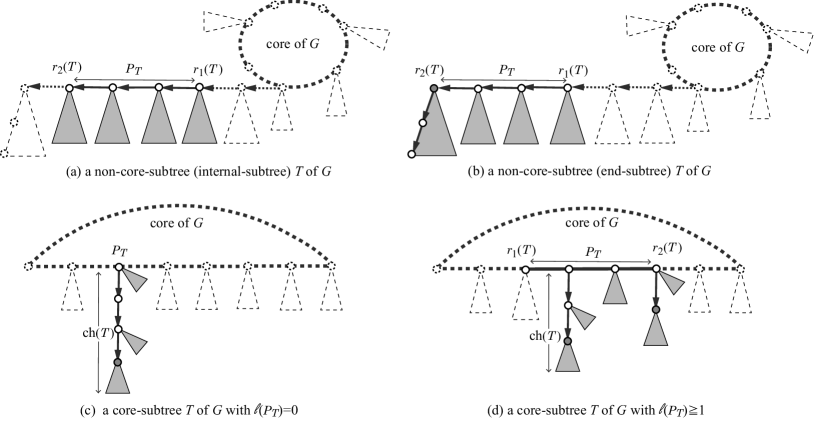
Figure 12: An illustration of subtrees of a chemical ${\rho}$-lean cyclic graph $G$, where thick lines depict the cycle of the core of $G$, gray circles depict leaf ${\rho}$-branches in $G$ and arrows depict non-core directed edges: (a) A non-core-subtree (internal-subtree) $T$ of $G$ represented by an nc-tree (a chemical bi-rooted tree); (b) A non-core-subtree (end-subtree) $T$ of $G$ represented by an nc-tree (a chemical bi-rooted tree); (c)  A core-subtree $T$ of $G$ with $\ell(P_{T})=0$ represented by a c-tree (a chemical rooted tree); (d) A core-subtree $T$ of $G$ with $\ell(P_{T})\geq 1$ represented by a c-tree (a chemical bi-rooted tree).

Fictitious Trees For an nc-tree or a c-tree $T$ and an integer $\Delta\in[1,3]$, let $T[+\Delta]$ denote a fictitious chemical graph obtained from $T$ by regarding the degree of terminal $r_{1}(T)$ as $\deg_{T}(r_{1}(T))+\Delta$. Figure 13(a) and (b) illustrate fictitious trees $T[+\Delta]$ in the case of $r_{1}(T)=r_{2}(T)$ and $T[+1]$ in the case of $\Delta=1$ and $r_{1}(T)\neq r_{2}(T)$.

For a c-tree $T$ with $r_{1}(T)\neq r_{2}(T)$ and integers $\Delta_{1},\Delta_{2}\in[1,3]$, let $T[+\Delta_{1},\Delta_{2}]$ denote a fictitious chemical graph obtained from $T$ by regarding the degree of terminal $r_{i}(T)$, $i=1,2$ as $\deg_{T}(r_{i}(T))+\Delta_{i}$. Figure 13(c) illustrates a fictitious bi-rooted c-tree $T[+\Delta_{1},\Delta_{2}]$.

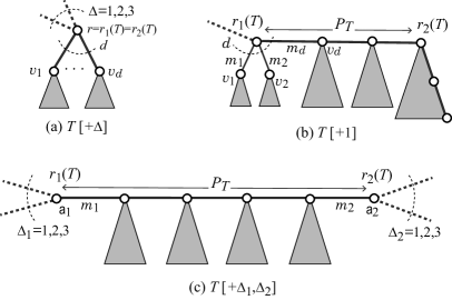
Figure 13: An illustration of fictitious trees: (a) $T[+\Delta]$ of a rooted nc- or c-tree $T$; (b) $T[+1]$ of a bi-rooted nc-tree $T$; (c) $T[+\Delta_{1},\Delta_{2}]$ of a bi-rooted c-tree $T$.

6.3 Frequency Vectors

For a finite set $A$ of elements, let $\mathbb{Z}_{+}^{A}$ denote the set of functions $\boldsymbol{w}:A\to\mathbb{Z}_{+}$. A function $\boldsymbol{w}\in\mathbb{Z}_{+}^{A}$ is called a non-negative integer vector (or a vector) on $A$ and the value $\boldsymbol{x}(a)$ for an element $a\in A$ is called the entry of $\boldsymbol{x}$ for $a\in A$. For a vector $\boldsymbol{w}\in\mathbb{Z}_{+}^{A}$ and an element $a\in A$, let $\boldsymbol{w}+\boldsymbol{1}_{a}$ (resp., $\boldsymbol{w}-\boldsymbol{1}_{a}$) denote the vector $\boldsymbol{w}^{\prime}$ such that $\boldsymbol{w}^{\prime}(a)=\boldsymbol{w}(a)+1$ (resp., $\boldsymbol{w}^{\prime}(a)=\boldsymbol{w}(a)-1$) and $\boldsymbol{w}^{\prime}(b)=\boldsymbol{w}(b)$ for the other elements $b\in A\setminus\{a\}$. For a vector $\boldsymbol{w}\in\mathbb{Z}_{+}^{A}$ and a subset $B\subseteq A$, let $\boldsymbol{w}_{[B]}$ denote the projection of $\boldsymbol{w}$ to $B$; i.e., $\boldsymbol{w}_{[B]}\in\mathbb{Z}_{+}^{B}$ such that $\boldsymbol{w}_{[B]}(b)=\boldsymbol{w}(b)$, $b\in B$.

To introduce a “frequency vector” of a subgraph of a chemical cyclic graph, we define sets of symbols that correspond to some descriptors of a chemical cyclic graph. Let $\Gamma^{\mathrm{co}}$, $\Gamma^{\mathrm{in}}$ and $\Gamma^{\mathrm{ex}}$ be sets of edge-configurations in Section 2.2. We define a vector whose entry is the frequency of an edge-configuration in sets $\Gamma^{\mathrm{t}}$, $\mathrm{t}\in\{\mathrm{co},\mathrm{in},\mathrm{ex}\}$ or the number of ${\rho}$-branch-core-vertices. We use a symbol ${\tt bc}$ to denote the number of ${\rho}$-branch-core-vertices in our frequency vector. To distinguish edge-configurations from different sets among three sets $\Gamma^{\mathrm{t}}$, $\mathrm{t}\in\{\mathrm{co},\mathrm{in},\mathrm{ex}\}$, we use $\gamma^{\mathrm{t}}$ to denote the entry of an edge-configuration $\gamma\in\Gamma^{\mathrm{t}}$, $\mathrm{t}\in\{\mathrm{co},\mathrm{in},\mathrm{ex}\}$. We denote by $\langle\Gamma^{\mathrm{t}}\rangle$ the set of entries $\gamma^{\mathrm{t}}$, $\gamma\in\Gamma^{\mathrm{t}}$, $\mathrm{t}\in\{\mathrm{co},\mathrm{in},\mathrm{ex}\}$. Define the set of all entries of a frequency vector to be

$${\Sigma\triangleq\{{\tt bc}\}\cup\bigcup_{\mathrm{t}\in\{\mathrm{co},\mathrm{in},\mathrm{ex}\}}\langle\Gamma^{\mathrm{t}}\rangle.}$$

Given an nc-tree or c-tree $G$ or a chemical ${\rho}$-lean cyclic graph $G$, define the frequency vector $\boldsymbol{f}(G)$, to be a vector $\boldsymbol{w}\in\mathbb{Z}_{+}^{\Sigma}$ that consists of the following entries:

• $\boldsymbol{w}(\gamma^{\mathrm{co}})=|\{uv\in\widetilde{E}_{\mathrm{co}}\mid(\alpha(u),\deg_{G}(u),\alpha(v),\deg_{G}(v))\in\{({\tt a},i,{\tt b},j,m),({\tt b},j,{\tt a},i,m)\},\beta(uv)=m\}|$, $\gamma=({\tt a}i,{\tt b}j,m)^{\mathrm{co}}\in\langle\Gamma^{\mathrm{co}}\rangle$;

• $\boldsymbol{w}(\gamma^{\mathrm{t}})=|\{(u,v)\in\widetilde{E}_{\mathrm{t}}\mid\alpha(u)={\tt a},\deg_{G}(u)=i,\alpha(v)={\tt b},\deg_{G}(v)=j,\beta(uv)=m\}|$, $\gamma=({\tt a}i,{\tt b}j,m)^{\mathrm{t}}\in\langle\Gamma^{\mathrm{t}}\rangle$, $\mathrm{t}\in\{\mathrm{in},\mathrm{ex}\}$;

• $\boldsymbol{w}({\tt bc})=\mathrm{bc}_{\rho}(G)$.

Note that any other descriptors of a chemical ${\rho}$-lean cyclic graph $G\in\mathcal{G}(\boldsymbol{x}^{*})$ except for the core height can be determined by the entries of the frequency vector $\boldsymbol{w}=\boldsymbol{f}(G)$. For example, the vector $\boldsymbol{z}\in\mathbb{Z}_{+}^{\{\mathrm{dg}1,\mathrm{dg}2,\mathrm{dg}3,\mathrm{dg}4\}}$ with the numbers $\mathrm{dg}i$ of core-vertices of degree $i\in[1,4]$ is given by

$${\boldsymbol{z}=\frac{1}{2}\Bigl{[}\sum_{\gamma^{\mathrm{co}}=({\tt a}i,{\tt a}j,m)^{\mathrm{co}}\in\langle\Gamma^{\mathrm{co}}\rangle}\!\!\!\!\boldsymbol{w}(\gamma^{\mathrm{co}})\cdot(\boldsymbol{1}_{\mathrm{dg}i}\!+\!\boldsymbol{1}_{\mathrm{dg}j})-\sum_{i_{v}=\deg_{G}(v):v\in V_{B}}(\Delta_{v}\!-\!2)\boldsymbol{1}_{\mathrm{dg}i_{v}}\Bigr{]}}$$

and the vector $\boldsymbol{z}^{\prime}\in\mathbb{Z}_{+}^{\Lambda_{\mathrm{dg}}}$ with the numbers of symbols $\mu\in\Lambda_{\mathrm{dg}}$ of core-vertices is given by

$${\boldsymbol{z}^{\prime}=\frac{1}{2}\Bigl{[}\sum_{\gamma^{\mathrm{co}}=(\mu,\xi,m)^{\mathrm{co}}\in\langle\Gamma^{\mathrm{co}}\rangle}\!\!\!\!\boldsymbol{w}(\gamma^{\mathrm{co}})\cdot(\boldsymbol{1}_{\mu}\!+\!\boldsymbol{1}_{\xi})-\sum_{\mu_{v}={\tt a}_{v}\deg_{G}(v):v\in V_{B}}(\Delta_{v}\!-\!2)\boldsymbol{1}_{\mu_{v}}\Bigr{]}.}$$

Similarly the vector $\boldsymbol{z}^{\prime\prime}\in\mathbb{Z}_{+}^{\Lambda_{\mathrm{dg}}}$ the numbers of symbols $\mu\in\Lambda_{\mathrm{dg}}$ of non-core-vertices is given by

$${\boldsymbol{z}^{\prime}=\sum_{\gamma^{\mathrm{in}}=(\mu,\xi,m)^{\mathrm{in}}\in\langle\Gamma^{\mathrm{in}}\rangle}\!\!\!\!\boldsymbol{w}(\gamma^{\mathrm{in}})\cdot\boldsymbol{1}_{\xi}+\sum_{\gamma^{\mathrm{ex}}=(\mu,\xi,m)^{\mathrm{ex}}\in\langle\Gamma^{\mathrm{ex}}\rangle}\!\!\!\!\boldsymbol{w}(\gamma^{\mathrm{ex}})\cdot\boldsymbol{1}_{\xi}.}$$

For an nc-tree or c-tree $T$, the frequency vector $\boldsymbol{f}(T[+\Delta])$ of a fictitious tree $T[+\Delta]$ is defined as follows: Let $r=r_{1}(T)$, $d=\deg_{T}(r)$, $N_{T}(r)=\{v_{1},v_{2},\ldots,v_{d}\}$, $\gamma_{j}=(\mu_{j}={\tt a}_{j}d,\xi_{j},m_{j})=\tau((r,v_{i}))\in\Gamma$, $j\in[1,d]$. Let $\widetilde{\gamma}_{j}=({\tt a}_{j}\{d\!+\!\Delta\},\xi_{j},m_{j})$, $j\in[1,d]$. Set $\mathrm{t}:=\mathrm{in}$ if $T$ is an nc-tree, and $\mathrm{t}:=\mathrm{co}$ if $T$ is a c-tree. When $r_{1}(T)=r_{2}(T)$,

$$\boldsymbol{f}(T[+\Delta])=\boldsymbol{f}(T)+\sum_{j\in[1,d]}(\boldsymbol{1}_{\widetilde{\gamma}_{j}^{\mathrm{t}}}-\boldsymbol{1}_{\gamma_{j}^{\mathrm{t}}}).$$

Let $r_{1}(T)\neq r_{2}(T)$, and $v_{d}$ belong to $P_{T}$. When $T$ is an nc-tree,

$$\boldsymbol{f}(T[+\Delta])=\boldsymbol{f}(T)+\sum_{j\in[1,d-\!1]}(\boldsymbol{1}_{\widetilde{\gamma}_{j}^{\mathrm{ex}}}-\boldsymbol{1}_{\gamma_{j}^{\mathrm{ex}}})+\boldsymbol{1}_{\widetilde{\gamma}_{d}^{\mathrm{in}}}-\boldsymbol{1}_{\gamma_{d}^{\mathrm{in}}}.$$

The frequency vector $\boldsymbol{f}(T[+\Delta_{1},\Delta_{2}])$ of a fictitious tree $T[+\Delta_{1},\Delta_{2}]$ for a bi-rooted c-tree $T$ with $r_{1}(T)\neq r_{2}(T)$ is defined as follows: For each $i=1,2$, let $r_{i}=r_{i}(T)$, ${\tt a}_{i}=\alpha(r_{i})$, $d_{i}=\deg_{T}(r_{i})$, $m_{i}=\beta(e_{i})$ of the unique edge incident to $r_{i}$ and $\gamma_{i}=(\mu_{i}={\tt a}_{i}d_{i},\xi_{i},m_{i})=\tau(e_{i})\in\Gamma$, $i=1,2$. Let $\widetilde{\gamma}_{i}=({\tt a}_{i}\{d_{i}\!+\!\Delta_{i}\},\xi_{i},m_{i})$, $i=1,2$. Then

$$\boldsymbol{f}(T[+\Delta_{1},\Delta_{2}])=\boldsymbol{f}(T)+\sum_{i=1,2}(\boldsymbol{1}_{\widetilde{\gamma}_{i}^{\mathrm{co}}}-\boldsymbol{1}_{\gamma_{i}^{\mathrm{co}}}).$$

6.4 A Chemical Graph Isomorphism

For a chemical ${\rho}$-lean cyclic graph for a branch-parameter ${\rho}\geq 1$, we choose a path-partition $\mathcal{P}=\{P_{1},P_{2},\ldots,P_{p}\}$ of the core $\mathrm{Cr}(H)=(V^{\mathrm{co}},E^{\mathrm{co}})$, where $|\mathcal{P}|\leq|E^{\mathrm{co}}|$. Let $V_{B}$ denote the set of all end-vertices of paths $P\in\mathcal{P}$, where $V_{\rho}^{\mathrm{bc}}\subseteq V_{B}\subseteq V^{\mathrm{co}}$.

Define the base-graph $G_{B}=(V_{B},E_{B})$ of $H$ by $\mathcal{P}$ to be the multigraph obtained from $H$ replacing each path $P_{j}\in\mathcal{P}$ with a single edge $e_{j}$ joining the end-vertices of $P_{i}$, where $E_{B}=\{e_{1},e_{2},\ldots,e_{p}\}$. We call a vertex in $V_{B}$ and an edge in $E_{B}$ a base-vertex and a base-edge, respectively. For a notational convenience in distinguishing the two end-vertices $u$ and $v$ of a base-edge $e=uv\in E_{B}$, we regard each base edge $e=uv$ as a directed edge $e=(u,v)$. For each base-edge $e\in E_{B}$, let $P_{e}$ denote the path $P_{j}\in E_{B}$ that is replaced by edge $e=e_{j}$.

We define the “components” of $G$ by $\mathcal{P}$ as follows.

Vertex-components For each base-vertex $v\in V_{B}$, define the component at vertex $v$ (or the $v$-component) $T_{v}$ of $G$ to be the chemical core-subtree rooted at $v$ in $G$; i.e., $T_{v}$ consists of all pendent-trees rooted at $v$. We regard $T_{v}$ as a c-tree rooted at the core-vertex $v$ of $G$ and define the code $\mathrm{code}_{v}(T_{v})$ of $T_{v}$ to be a tuple $({\tt a}_{v},d_{v},m_{v},\Delta_{v},\boldsymbol{x}_{v})$ such that

$${\tt a}_{v}=\alpha(v) d_{v}=\deg_{G}(v)-\deg_{G_{B}}(v) m_{v}=\sum_{vv^{\prime}\in E(T_{v})}\beta(vv^{\prime})$$, , ,

$$\Delta_{v}=\deg_{G_{B}}(v) \boldsymbol{x}_{v}=\boldsymbol{f}(T_{v}[+\Delta_{v}])$$ and .

Edge-components For each base-edge $e=e_{j}=(u,v)\in E_{B}$, define the component at edge $e$ (or the $e$-component) $T_{e}$ of $G$ to be the chemical core-subtree of $G$ that consists of the core-path $P_{j}\in\mathcal{P}$ and all pendant-trees of $G$ rooted at internal vertices of path $P_{j}$. We regard $T_{e}$ as a bi-rooted c-tree with $r_{1}(T_{e})=u$ and $r_{2}(T_{e})=v$ for the base-edge $e=uv$ and define the code $\mathrm{code}_{e}(T_{e})$ of $T_{e}$ to be a tuple $({\tt a}_{u}^{e},m_{u}^{e},{\tt a}_{v}^{e},m_{v}^{e},\Delta_{u}^{e},\Delta_{v}^{e},\boldsymbol{x}_{e})$ such that

$${\tt a}_{u}^{e}=\alpha(u) {\tt a}_{v}^{e}=\alpha(v) \Delta_{u}^{e}=\deg_{G_{B}}(u)-1 \Delta_{v}^{e}=\deg_{G_{B}}(v)-1$$, , , ,

$$\boldsymbol{x}_{e}=\boldsymbol{f}(T_{e}[+\Delta_{u}^{e},\Delta_{v}^{e}])$$,

$$m_{u}^{e}=\beta(uu^{\prime}) m_{v}^{e}=\beta(vv^{\prime}) uu^{\prime},vv^{\prime}\in E(P_{j}) u v$$ and for the edges incident to and .

Observe that

$$\boldsymbol{f}(G)=\sum_{v\in V_{B}}\boldsymbol{x}_{v}+\sum_{e\in E_{B}}\boldsymbol{x}_{e}.$$

We introduce a specification $\sigma_{\mathrm{ch}}$ as a set of functions $\mathrm{ch}_{\mathrm{LB}}:V_{B}\cup E_{B}\to\mathbb{Z}_{+}$.

We call two chemical graphs $(\mathcal{P},\sigma_{\mathrm{ch}})$-isomorphic if they consist of vertex and edge components with the same codes and heights; i.e., two chemical ${\rho}$-lean cyclic graphs $G^{i}=(H^{i},\alpha^{i},\beta^{i})$, $i=1,2$ are $(\mathcal{P},\sigma_{\mathrm{ch}})$-isomorphic if the following hold:

1. $\mathrm{Cr}(H_{1})$ and $\mathrm{Cr}(H_{2})$ are graph-isomorphic, where we assume that $\mathrm{Cr}(H_{1})=\mathrm{Cr}(H_{2})=(V^{\mathrm{co}},E^{\mathrm{co}})$ and $G_{B}=(V_{B},E_{B})$ denotes the base-graph of both graphs $H_{1}$ and $H_{2}$ by $\mathcal{P}$;

2. For the $v$-components $T^{i}_{v}$ of $G^{i}$, $i=1,2$ at each base-vertex $v\in V_{B}$,

   $$\mathrm{code}_{v}(T^{1}_{v})=\mathrm{code}_{v}(T^{2}_{v})\mbox{ and }\mathrm{ht}(T^{2}_{v}),\mathrm{ht}(T^{1}_{v})\in[\mathrm{ch}_{\mathrm{LB}}(v),\mathrm{ch}_{\mathrm{UB}}(v)];$$

3. For the $e$-components $T^{i}_{e}$ of $G^{i}$, $i=1,2$ at each base-edge $e\in E_{B}$,

   $$\mathrm{code}_{e}(T^{1}_{e})=\mathrm{code}_{e}(T^{2}_{e})\mbox{ and }\mathrm{ht}(T^{2}_{v}),\mathrm{ht}(T^{1}_{v})\in[\mathrm{ch}_{\mathrm{LB}}(v),\mathrm{ch}_{\mathrm{UB}}(v)];$$

See Section 2 for the definition of height $\mathrm{ht}(T)$ of a bi-rooted tree $T$.

The $(\mathcal{P},\sigma_{\mathrm{ch}})$-isomorphism also implies that $\boldsymbol{f}(G^{1})=\boldsymbol{f}(G^{2})$, $n(G^{1})=n(G^{2})$, $\mathrm{cs}(G^{1})=\mathrm{cs}(G^{2})$, $\mathrm{bl}_{\rho}(G^{1})=\mathrm{bc}_{\rho}(G^{1})=\mathrm{bl}_{\rho}(G^{2})=\mathrm{bc}_{\rho}(G^{2})$ and $|\mathrm{ch}(G^{1})-\mathrm{ch}(G^{2})|\leq\max_{\mathrm{t}\in V_{B}\cup E_{B}}(\mathrm{ch}_{\mathrm{UB}}(\mathrm{t})-\mathrm{ch}_{\mathrm{LB}}(\mathrm{t}))$.

6.5 Computing Isomorphic Chemical Graphs from a Given Chemical Graph $\mathcal{G}^{\dagger}$

Now we assume that a chemical ${\rho}$-lean cyclic graph $G^{\dagger}$ for a branch-parameter ${\rho}\geq\mathrm{ch}(G^{\dagger})$ is available in such case where a target chemical graph $G^{\dagger}$ is constructed by solving an MILP in Stage 4. Let $T_{v}^{\dagger}$ (resp., $T_{e}^{\dagger}$) denote the $v$-component (resp., the $e$-component) of $G^{\dagger}$.

Target $v$-components Let $\mathrm{ht}^{*}_{v}$ denote the height $h(T^{\dagger}_{v})$ of the $v$-component of $G^{\dagger}$. For each base-vertex $v\in V_{B}$, fix a code $({\tt a}_{v},d_{v},m_{v},\Delta_{v},\boldsymbol{x}^{*}_{v}):=\mathrm{code}_{v}(T^{\dagger}_{v})$ and call a rooted c-tree $T$ a target $v$-component if

$$\mathrm{code}_{v}(T)=({\tt a}_{v},d_{v},m_{v},\Delta_{v},\boldsymbol{x}_{v}^{*}) \mathrm{ht}(T)\in[\mathrm{ch}_{\mathrm{LB}}(v),\mathrm{ch}_{\mathrm{UB}}(v)]$$ and ,

where the condition on $\mathrm{ht}(T)$ is equivalent to $\mathrm{ht}(T)=\mathrm{ht}^{*}_{v}$ when $\boldsymbol{x}^{*}_{v}({\tt bc})=1$, since $G^{\dagger}$ is a ${\rho}$-lean cyclic graph and the set of ${\rho}$-internal edges in any target component forms a single path of length $\mathrm{ht}^{*}_{v}$ from the root to a unique leaf ${\rho}$-branch.

Target $e$-components For each base-edge $e=(u,v)=e_{j}\in E_{B}$, fix a code $({\tt a}_{u}^{e},m_{u}^{e},{\tt a}_{v}^{e},m_{v}^{e},$ $\Delta_{u}^{e},\Delta_{v}^{e},\boldsymbol{x}_{e}^{*}):=\mathrm{code}_{e}(T^{\dagger}_{e})$ and call a bi-rooted c-tree $T$ a target $e$-component if

$$\mathrm{code}_{e}(T)=({\tt a}_{u}^{e},m_{u}^{e},{\tt a}_{v}^{e},m_{v}^{e}, \Delta_{u}^{e},\Delta_{v}^{e},\boldsymbol{x}_{e}^{*}) \mathrm{ht}(T)\in[\mathrm{ch}_{\mathrm{LB}}(e),\mathrm{ch}_{\mathrm{UB}}(e)]$$ and .

Let $\mathcal{T}_{e}$ denote the set of all target components of a base-edge $e\in E_{B}$.

Given a collection of target $v$-components $T_{v}\in\mathcal{T}_{v}$, $v\in V_{B}$ and target $e$-components $T_{e}\in\mathcal{T}_{e}$, $e\in E_{B}$, there is a chemical ${\rho}$-lean cyclic graph $G^{*}$ that is $(\mathcal{P},\sigma_{\mathrm{ch}})$-isomorphic to the original chemical graph $G^{\dagger}$. Such a graph $G^{*}$ can be obtained from $G_{B}$ by replacing each base-edge $e\in E_{B}$ with $T_{e}$ and attaching $T_{v}$ at each base-vertex $v\in V_{B}$.

From this observation, our aim is now to generate some number of target $v$-components for each base-vertex $v$ and target $e$-components for each base-edge $e$. In the following, we denote ${\tt a}_{u}^{e}$, ${\tt a}_{v}^{e}$, $\Delta_{u}^{e}$, $\Delta_{v}^{e}$, $m_{u}^{e}$ and $m_{v}^{e}$ for each base-edge $e=(u,v)\in E_{B}$ by ${\tt a}_{1}^{e}$, ${\tt a}_{2}^{e}$, $\Delta_{1}^{e}$, $\Delta_{2}^{e}$, $m_{1}^{e}$ and $m_{2}^{e}$, respectively for a notational simplicity. For each base-edge $e=e_{j}\in E_{B}$, let

$$\delta_{1}^{e}:=\lfloor(\ell(P_{j})-1)/2\rfloor\mbox{ and }\delta_{2}^{e}:=\lceil(\ell(P_{j})-1)/2\rceil.$$

6.5.1 Dynamic Programming Algorithm on Frequency Vectors

We start with describing a sketch of our new algorithm for generating graphs $G^{*}$ in Stage 5 before we present some technical details of the algorithm in the following sections.

We start with enumerating chemical rooted trees with height at most ${\rho}$, which can be a ${\rho}$-fringe-tree of a target component. Next we extend each of the rooted tree to an nc-tree $T$ and then to a c-tree $T$ under a constraint that the frequency vector of $T$ does not exceed a given vector $\boldsymbol{x}=\boldsymbol{x}^{*}_{v}$, $v\in V_{B}$ or $\boldsymbol{x}=\boldsymbol{x}^{*}_{e}$, $e\in E_{B}$.

For a vector $\boldsymbol{x}\in\mathbb{Z}_{+}^{\Sigma}$, we formulate the following sets of nc-trees and c-trees and of their frequency vectors:

1. $\mathcal{T}_{\mathrm{inl}}^{(0)}({\tt a},d,m;\boldsymbol{x})$, ${\tt a}\in\Lambda$, $d\in[0,\min\{\mathrm{val}({\tt a}),d_{\max}\}-2]$, $m\in[d,\mathrm{val}({\tt a})-2]$: the set of rooted nc-trees $T$ with a root $r$ such that

   $$\alpha(r)={\tt a} \deg_{T}(r)=d \beta_{T}(r)=m \mathrm{ht}(T)\leq{\rho} \boldsymbol{f}(T[+2])\leq\boldsymbol{x}$$, , , and ;

   Let $\mathrm{W}_{\mathrm{inl}}^{(0)}({\tt a},d,m;\boldsymbol{x})$ denote the set of the frequency vectors $\boldsymbol{w}=\boldsymbol{f}(T[+2])$ for all nc-trees $T\in\mathcal{T}_{\mathrm{inl}}^{(0)}({\tt a},d,m;\boldsymbol{x})$;

2. $\mathcal{T}_{\mathrm{end}}^{(0)}({\tt a},d,m;\boldsymbol{x})$, ${\tt a}\in\Lambda$, $d\in[1,\min\{\mathrm{val}({\tt a}),d_{\max}\}-1]$, $m\in[d,\mathrm{val}({\tt a})-1]$: the set of rooted nc-trees $T$ with a root $r$ such that

   $$\alpha(r)={\tt a} \deg_{T}(r)=d \beta_{T}(r)=m \mathrm{ht}(T)={\rho} \boldsymbol{f}(T[+1])\leq\boldsymbol{x}$$, , , and ;

   Let $\mathrm{W}_{\mathrm{end}}^{(0)}({\tt a},d,m;\boldsymbol{x})$ denote the set of the frequency vectors $\boldsymbol{w}=\boldsymbol{f}(T[+1])$ for all nc-trees $T\in\mathcal{T}_{\mathrm{end}}^{(0)}({\tt a},d,m;\boldsymbol{x})$;

3. $\mathcal{T}_{\mathrm{end}}^{(h)}({\tt a},d,m;\boldsymbol{x})$, $\boldsymbol{x}=\boldsymbol{x}_{\mathrm{t}}^{*}$, ${\tt a}\in\Lambda$, $d\in[1,\min\{\mathrm{val}({\tt a}),d_{\max}\}-1]$, $m\in[d,\mathrm{val}({\tt a})-1]$, $h\in[1,\mathrm{ch}_{\mathrm{UB}}(\mathrm{t})]$: the set of bi-rooted nc-trees $T$ such that

   $$\alpha(r_{1}(T))={\tt a} \deg_{T}(r_{1}(T))=d \beta(r_{1}(T))=m \ell(P_{T})=h \boldsymbol{f}(T[+1])\leq\boldsymbol{x}$$, , , , ,

   $$\mathrm{ht}(T^{\prime})\leq{\rho} T^{\prime}\in\mathcal{F}(T)$$ for all trees and

   $$\mathrm{ht}(T^{\prime\prime})={\rho} T^{\prime\prime}\in\mathcal{F}(T) r_{2}(T)$$ for the tree rooted at terminal ;

   Let $\mathrm{W}_{\mathrm{end}}^{(h)}({\tt a},d,m)$ denote the set of all frequency vectors $\boldsymbol{w}=\boldsymbol{f}(T[+1])$ for all bi-rooted nc-trees $T\in\mathcal{T}_{\mathrm{end}}^{(h)}({\tt a},d,m)$;

4. $\mathcal{T}_{\mathrm{co}+\Delta}^{(0)}({\tt a},d,m,h;\boldsymbol{x})$, $\boldsymbol{x}=\boldsymbol{x}_{\mathrm{t}}^{*}$, ${\tt a}\in\Lambda$, $\Delta\in[2,3]$, $d\in[0,\min\{\mathrm{val}({\tt a}),d_{\max}\}-\Delta]$, $m\in[d,\mathrm{val}({\tt a})-\Delta]$, $h\in[0,\mathrm{ch}_{\mathrm{UB}}(\mathrm{t})]$: the set of rooted c-trees $T$ with a root $r$ such that

   $$\alpha(r)={\tt a} \deg_{T}(r)=d \beta_{T}(r)=m \mathrm{ht}(T)=h \boldsymbol{f}(T[+\Delta])\leq\boldsymbol{x}$$, , , and ;

   Let $\mathrm{W}_{\mathrm{co}+\Delta}^{(0)}({\tt a},d,m,h;\boldsymbol{x})$ denote the set of the frequency vectors $\boldsymbol{w}=\boldsymbol{f}(T[+\Delta])$ for all c-trees $T\in\mathcal{T}_{\mathrm{co}+\Delta}^{(0)}({\tt a},d,m,h;\boldsymbol{x})$;

5. $\mathcal{T}_{\mathrm{co}+1,\Delta}^{(q)}({\tt a},d,m,{\tt b},1,m^{\prime},h;\boldsymbol{x})$, $\boldsymbol{x}=\boldsymbol{x}_{e}^{*}$, ${\tt a},{\tt b}\in\Lambda$, $\Delta\in[2,3]$, $d\in[1,\min\{\mathrm{val}({\tt a}),d_{\max}\}-1]$, $m\in[d,\mathrm{val}({\tt a})-1]$, $m^{\prime}\in[1,\mathrm{val}({\tt b})-\Delta]$, $h\in[0,\mathrm{ch}_{\mathrm{UB}}(e)]$, $q\in[1,\ell(P_{e})]$: the set of bi-rooted c-trees $T$ such that

   $$\alpha(r_{1}(T))={\tt a} \deg_{T}(r_{2}(T))=1 \beta(r_{1}(T))=m$$, , ,

   $$\alpha(r_{2}(T))={\tt b} \deg_{T}(r_{1}(T))=d \beta(r_{2}(T))=m^{\prime}$$, , ,

   $$\ell(P_{T})=q \mathrm{ht}(T)=h \boldsymbol{f}(T[+1,\Delta])\leq\boldsymbol{x}$$, and ;

   Let $\mathrm{W}_{\mathrm{co}+1,\Delta}^{(q)}({\tt a},d,m,{\tt b},1,m^{\prime},h;\boldsymbol{x})$ denote the set of the frequency vectors $\boldsymbol{w}=\boldsymbol{f}(T[+1,\Delta])$ for all bi-rooted c-trees $T\in\mathcal{T}_{\mathrm{co}+1,\Delta}^{(q)}({\tt a},d,m,{\tt b},1,m^{\prime},h;\boldsymbol{x})$.

Note that $\boldsymbol{w}({\tt bc})=0$ for any vector $\boldsymbol{w}$ in the above set in (i)-(iii).

Our algorithm consists of six steps. Step 1 computes the sets of trees and vectors in (i), (ii) and (iii) with $h\leq{\rho}$, where each tree in these sets is of height at most ${\rho}$. Note that the frequency vectors of some two trees in a tree set $\mathcal{T}$ in the above can be identical. In fact, the size $|\mathcal{T}|$ of a set $\mathcal{T}$ of trees can be considerably larger than that $|\mathrm{W}|$ of the set $\mathrm{W}$ of their frequency vectors. We mainly maintain a whole vector set $\mathrm{W}$, and for each vector $\boldsymbol{w}\in\mathrm{W}$, we store at least one tree $T_{\boldsymbol{w}}\in\mathcal{T}$ such that $\boldsymbol{w}$ is the frequency vector of a fictitious tree of $T_{\boldsymbol{w}}$, where we call such a tree $T_{\boldsymbol{w}}$ a sample tree of the vector $\boldsymbol{w}$. With this idea, Steps 2-5 compute only vector sets $\mathrm{W}$ in (iii) with $h>{\rho}$, (iv) and (v). In each of these steps, we compute a set $\mathcal{S}$ of sample trees of the vectors in each vector set $\mathrm{W}$. The last step constructs at least one target component for each base-vertex or base-edge, and then combines them to obtain a graph $G^{*}$ to be inferred in Stage 5.

We derive recursive formula that hold among the above sets. Based on this, we compute the vector sets in (iii) in Step 2, those in (iv) in Step 3 and those in (v) in Step 4. During these steps, we can find a target $v$-component for each base-vertex $v\in V_{B}$. For each base-edge $e=(u_{1},u_{2})\in E_{B}$, Step 5 compare vectors $\boldsymbol{w}_{1}$ and $\boldsymbol{w}_{2}$, where $\boldsymbol{w}_{i}$ is the frequency vector of a c-tree $T_{i}$ that is extended from the end-vertex $u_{i}$, to examine whether $T_{1}$ and $T_{2}$ give rise to a target $e$-component.

6.5.2 Step 1: Enumeration of ${\rho}$-fringe-trees

Step 1 computes the following sets in (i)-(iv).

1. For each base-vertex $v\in V_{B}$ such that $\mathrm{ch}_{\mathrm{LB}}(v)\leq{\rho}$ and $\boldsymbol{x}^{*}_{v}({\tt bc})=0$, compute the set $\mathcal{T}_{\mathrm{co}+\Delta_{v}}^{(0)}({\tt a}_{v},d_{v},m_{v},h;\boldsymbol{x}^{*}_{v})$, $h\in[\mathrm{ch}_{\mathrm{LB}}(v),\min\{{\rho},\mathrm{ch}_{\mathrm{UB}}(v)\}]$ of rooted c-trees. Note that every c-tree in the set $\mathcal{T}_{\mathrm{co}+\Delta_{v}}^{(0)}({\tt a}_{v},d_{v},m_{v},h;\boldsymbol{x}^{*}_{v})$ with $h\in[\mathrm{ch}_{\mathrm{LB}}(v),\min\{{\rho},\mathrm{ch}_{\mathrm{UB}}(v)\}]$ is a target $v$-component in $\mathcal{T}_{v}$;
   Set $\mathcal{S}(v)$ be a subset of $\bigcup_{h\in[\mathrm{ch}_{\mathrm{LB}}(v),\min\{{\rho},\mathrm{ch}_{\mathrm{UB}}(v)\}]}\mathcal{T}_{\mathrm{co}+\Delta_{v}}^{(0)}({\tt a}_{v},d_{v},m_{v},h;\boldsymbol{x}^{*}_{v})$;

2. For each base-vertex $v\in V_{B}$ such that ${\rho}<\mathrm{ch}_{\mathrm{UB}}(v)$ and $\boldsymbol{x}^{*}_{v}({\tt bc})=1$ and integers $m\in[d_{v}-1,\mathrm{val}({\tt a}_{v})-\Delta_{v}-1]$ and $p\in[0,k]$, compute the sets $\mathcal{T}_{\mathrm{co}+(\Delta_{v}+1)}^{(0)}({\tt a}_{v},d_{v}-1,m,p;\boldsymbol{x}^{*}_{v})$ of rooted c-trees and $\mathrm{W}_{\mathrm{co}+(\Delta_{v}+1)}^{(0)}({\tt a}_{v},d_{v}-1,m,p;\boldsymbol{x}^{*}_{v})$ of their frequency vectors;
   For each vector $\boldsymbol{w}\in\mathrm{W}_{\mathrm{co}+(\Delta_{v}+1)}^{(0)}({\tt a}_{v},d_{v}-1,m,p;\boldsymbol{x}^{*}_{v})$, choose some number of sample trees $T_{\boldsymbol{w}}$, and store them in a set $\mathcal{S}_{\mathrm{co}+(\Delta_{v}+1)}^{(0)}({\tt a}_{v},d_{v}-1,m,p;\boldsymbol{x}^{*}_{v})$;

3. For each base-vertex $v\in V_{B}$ such that ${\rho}<\mathrm{ch}_{\mathrm{UB}}(v)$ and $\boldsymbol{x}^{*}_{v}({\tt bc})=1$, each possible tuple $({\tt a},d,m)$, compute the sets $\mathcal{T}_{\mathrm{inl}}^{(0)}({\tt a},d,m;\boldsymbol{x}^{*}_{v})$ and $\mathcal{T}_{\mathrm{end}}^{(0)}({\tt a},d,m;\boldsymbol{x}^{*}_{v})$ of rooted nc-trees and the sets $\mathrm{W}_{\mathrm{inl}}^{(0)}({\tt a},d,m;\boldsymbol{x}^{*}_{v})$ and $\mathrm{W}_{\mathrm{end}}^{(0)}({\tt a},d,m;\boldsymbol{x}^{*}_{v})$ of their frequency vectors;
   For each vector $\boldsymbol{w}\in\mathrm{W}_{\mathrm{inl}}^{(0)}({\tt a},d,m;\boldsymbol{x}^{*}_{v})$ (resp., $\boldsymbol{w}\in\mathrm{W}_{\mathrm{end}}^{(0)}({\tt a},d,m;\boldsymbol{x}^{*}_{v})$), choose some number of sample trees $T_{\boldsymbol{w}}\in\mathcal{T}_{\mathrm{co}+\Delta}^{(0)}({\tt a},d,m,h;\boldsymbol{x}^{*}_{e})$, and store them in a set $\mathcal{S}_{\mathrm{inl}}^{(0)}({\tt a},d,m;\boldsymbol{x}^{*}_{v})$ (resp., $\boldsymbol{w}\in\mathrm{W}_{\mathrm{end}}^{(0)}({\tt a},d,m;\boldsymbol{x}^{*}_{v})$);

4. For each base-edge $e\in E_{B}$ and each possible tuple $({\tt a},d,m)$, compute the sets $\mathcal{T}_{\mathrm{inl}}^{(0)}({\tt a},d,m;\boldsymbol{x}^{*}_{e})$ and $\mathcal{T}_{\mathrm{end}}^{(0)}({\tt a},d,m;\boldsymbol{x}^{*}_{e})$ of rooted nc-trees and $\mathcal{T}_{\mathrm{co}+\Delta}^{(0)}({\tt a},d,m,h;\boldsymbol{x}^{*}_{e})$, $h\in[0,\min\{{\rho},\mathrm{ch}_{\mathrm{UB}}(e)\}]$ of rooted c-trees and the sets $\mathrm{W}_{\mathrm{inl}}^{(0)}({\tt a},d,m;\boldsymbol{x}^{*}_{e})$, $\mathrm{W}_{\mathrm{end}}^{(0)}({\tt a},d,m;\boldsymbol{x}^{*}_{e})$ and $\mathrm{W}_{\mathrm{co}+\Delta}^{(0)}({\tt a},d,m,h;\boldsymbol{x}^{*}_{e})$ of their frequency vectors;
   For each vector $\boldsymbol{w}\in\mathrm{W}_{\mathrm{inl}}^{(0)}({\tt a},d,m;\boldsymbol{x}^{*}_{e})$ (resp., $\boldsymbol{w}\in\mathrm{W}_{\mathrm{end}}^{(0)}({\tt a},d,m;\boldsymbol{x}^{*}_{e})$ and $\boldsymbol{w}\in\mathrm{W}_{\mathrm{co}+\Delta}^{(0)}({\tt a},d,m,h;\boldsymbol{x}^{*}_{e})$), choose some number of sample trees $T_{\boldsymbol{w}}$ and store them in a set $\mathcal{S}_{\mathrm{inl}}^{(0)}({\tt a},d,m;\boldsymbol{x}^{*}_{e})$ (resp., $\mathcal{S}_{\mathrm{end}}^{(0)}({\tt a},d,m;\boldsymbol{x}^{*}_{e})$ and $\mathcal{S}_{\mathrm{co}+\Delta}^{(0)}({\tt a},d,m,h;\boldsymbol{x}^{*}_{e})$),

To compute the above sets of trees and vectors, we enumerate all possible trees with height at most 2 under the size constraint (1) by a branch-and-bound procedure.

6.5.3 Step 2: Generation of Frequency Vectors of End-subtrees

For each base-vertex $\mathrm{t}=v\in V_{B}$ or each base-edge $\mathrm{t}=e\in E_{B}$ such that ${\rho}<\mathrm{ch}_{\mathrm{UB}}(\mathrm{t})$ and each possible tuple $({\tt a},d,m)$, Step 2 computes the set $\mathrm{W}_{\mathrm{end}}^{(h)}({\tt a},d,m;\boldsymbol{x}^{*}_{\mathrm{t}})$ in the ascending order of $h=1,2,\ldots,\mathrm{ch}_{\mathrm{UB}}(\mathrm{t})-{\rho}-1$. Observe that each vector $\boldsymbol{w}\in\mathrm{W}_{\mathrm{end}}^{(h)}({\tt a},d,m;\boldsymbol{x}^{*}_{\mathrm{t}})$ is obtained as $\boldsymbol{w}=\boldsymbol{w}^{\prime}+\boldsymbol{w}^{\prime\prime}+\boldsymbol{1}_{\gamma^{\mathrm{in}}}$ from a combination of vectors $\boldsymbol{w}^{\prime}\in\mathrm{W}_{\mathrm{inl}}^{(0)}({\tt a},d-1,m^{\prime};\boldsymbol{x}^{*}_{\mathrm{t}})$ and $\boldsymbol{w}^{\prime\prime}\in\mathrm{W}_{\mathrm{end}}^{(h-1)}({\tt b},d^{\prime\prime},m^{\prime\prime};\boldsymbol{x}^{*}_{\mathrm{t}})$ such that

$$\begin{array}[]{l}m^{\prime}\leq\mathrm{val}({\tt a})-2,~{}~{}1\leq m-m^{\prime}\leq\mathrm{val}(b)-m^{\prime\prime},\\ \boldsymbol{w}^{\prime}+\boldsymbol{w}^{\prime\prime}+\boldsymbol{1}_{\gamma^{\mathrm{in}}}\leq\boldsymbol{x}^{*}_{\mathrm{t}}\mbox{ for }\gamma=({\tt a}\{d\!+\!1\},{\tt b}\{d^{\prime\prime}\!+\!1\},m-m^{\prime})\in\Gamma.\end{array}$$

Figure 14(a) illustrates this process of computing a vector $\boldsymbol{w}\in\mathrm{W}_{\mathrm{end}}^{(h)}({\tt a},d,m;\boldsymbol{x}^{*}_{\mathrm{t}})$.

For each vector $\boldsymbol{w}\in\mathrm{W}_{\mathrm{end}}^{(h)}({\tt a},d,m;\boldsymbol{x}^{*}_{\mathrm{t}})$ obtained from a combination $\boldsymbol{w}^{\prime}\in\mathrm{W}_{\mathrm{inl}}^{(0)}({\tt a},d-1,m^{\prime};\boldsymbol{x}^{*}_{\mathrm{t}})$ and $\boldsymbol{w}^{\prime\prime}\in\mathrm{W}_{\mathrm{end}}^{(h-1)}({\tt b},d^{\prime\prime},m^{\prime\prime};\boldsymbol{x}^{*}_{\mathrm{t}})$, we construct at least one sample nc-tree $T_{\boldsymbol{w}}$ from their sample nc-trees $T_{\boldsymbol{w}^{\prime}}\in\mathcal{S}_{\mathrm{inl}}^{(0)}({\tt a},d-1,m^{\prime};\boldsymbol{x}^{*}_{\mathrm{t}})$ and $T_{\boldsymbol{w}^{\prime\prime}}\in\mathcal{S}_{\mathrm{end}}^{(h-1)}({\tt b},d^{\prime\prime},m^{\prime\prime};\boldsymbol{x}^{*}_{\mathrm{t}})$ and store them in a set $\mathcal{S}_{\mathrm{end}}^{(h)}({\tt a},d,m;\boldsymbol{x}^{*}_{\mathrm{t}})$.

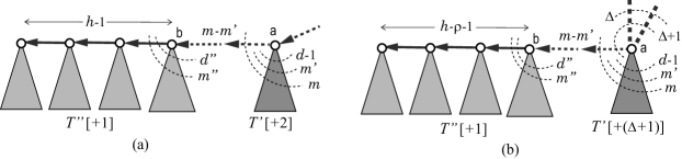
Figure 14: (a) An illustration of computing a vector $\boldsymbol{w}\in\mathrm{W}_{\mathrm{end}}^{(h)}({\tt a},d,m;\boldsymbol{x}^{*}_{\mathrm{t}})$ from the frequency vectors $\boldsymbol{w}^{\prime}=\boldsymbol{f}(T^{\prime}[+2])\in\mathrm{W}_{\mathrm{inl}}^{(0)}({\tt a},d-1,m^{\prime};\boldsymbol{x}^{*}_{\mathrm{t}})$ of a bi-rooted nc-tree $T^{\prime}$ and $\boldsymbol{w}^{\prime\prime}=\boldsymbol{f}(T^{\prime\prime}[+1])\in\mathrm{W}_{\mathrm{end}}^{(h-1)}({\tt b},d^{\prime\prime},m^{\prime\prime};\boldsymbol{x}^{*}_{\mathrm{t}})$ of an nc-tree $T^{\prime\prime}$; (b) An illustration of computing a vector $\boldsymbol{w}\in\mathrm{W}_{\mathrm{co}+\Delta}^{(0)}({\tt a},d,m,h;\boldsymbol{x}^{*}_{\mathrm{t}})$ from the frequency vectors $\boldsymbol{w}^{\prime}=\boldsymbol{f}(T^{\prime}[+(\Delta+1)])\in\mathrm{W}_{\mathrm{co}+(\Delta+1)}^{(0)}({\tt a},d-\!1,m^{\prime},p;\boldsymbol{x}^{*}_{\mathrm{t}})$, $p\in[0,{\rho}]$ of a c-tree $T^{\prime}$ and $\boldsymbol{w}^{\prime\prime}=\boldsymbol{f}(T^{\prime\prime}[+1])\in\mathrm{W}_{\mathrm{end}}^{(h-{\rho}-1)}({\tt b},d^{\prime\prime},m^{\prime\prime};\boldsymbol{x}^{*}_{\mathrm{t}})$.

6.5.4 Step 3: Generation of Frequency Vectors of Rooted Core-subtrees

For each base-vertex $\mathrm{t}=v\in V_{B}$ or each base-edge $\mathrm{t}=e\in E_{B}$ such that ${\rho}<\mathrm{ch}_{\mathrm{UB}}(\mathrm{t})$ and each possible tuple $({\tt a},d,m,h)$ with $h\in[{\rho}+1,\mathrm{ch}_{\mathrm{UB}}(\mathrm{t})]$, Step 3 computes the set $\mathrm{W}_{\mathrm{co}+\Delta}^{(0)}({\tt a},d,m,h;\boldsymbol{x}^{*}_{\mathrm{t}})$. Observe that each vector $\boldsymbol{w}\in\mathrm{W}_{\mathrm{co}+\Delta}^{(0)}({\tt a},d,m,h;\boldsymbol{x}^{*}_{\mathrm{t}})$ is obtained as $\boldsymbol{w}=\boldsymbol{w}^{\prime}+\boldsymbol{w}^{\prime\prime}+\boldsymbol{1}_{\gamma^{\mathrm{in}}}+\boldsymbol{1}_{{\tt bc}}$ from a combination of vectors $\boldsymbol{w}^{\prime}\in\mathrm{W}_{\mathrm{co}+(\Delta+1)}^{(0)}({\tt a},d-\!1,m^{\prime},p;\boldsymbol{x}^{*}_{\mathrm{t}})$, $p\in[0,k]$ and $\boldsymbol{w}^{\prime\prime}\in\mathrm{W}_{\mathrm{end}}^{(h-{\rho}-1)}({\tt b},d^{\prime\prime},m^{\prime\prime};\boldsymbol{x}^{*}_{\mathrm{t}})$ such that

$$\begin{array}[]{l}m^{\prime}\leq\mathrm{val}({\tt a})-\Delta-1,~{}~{}1\leq m-m^{\prime}\leq\mathrm{val}(b)-m^{\prime\prime},\\ \boldsymbol{w}^{\prime}+\boldsymbol{w}^{\prime\prime}+\boldsymbol{1}_{\gamma^{\mathrm{in}}}+\boldsymbol{1}_{{\tt bc}}\leq\boldsymbol{x}^{*}_{\mathrm{t}}\mbox{ for }\gamma=({\tt a}\{d\!+\!\Delta\},{\tt b}\{d^{\prime\prime}\!+\!1\},m-m^{\prime})\in\Gamma,\end{array}$$

where $\boldsymbol{w}^{\prime}({\tt bc})=\boldsymbol{w}^{\prime\prime}({\tt bc})=0$. Figure 14(b) illustrates this process of computing a vector $\boldsymbol{w}\in\mathrm{W}_{\mathrm{co}+\Delta}^{(0)}({\tt a},d,m,h;\boldsymbol{x}^{*}_{\mathrm{t}})$.

For each vector $\boldsymbol{w}\in\mathrm{W}_{\mathrm{co}+\Delta}^{(0)}({\tt a},d,m,h;\boldsymbol{x}^{*}_{\mathrm{t}})$ obtained from a combination of vectors
$\boldsymbol{w}^{\prime}\in\bigcup_{p\in[0,k]}\mathrm{W}_{\mathrm{co}+(\Delta+1)}^{(0)}({\tt a},d-\!1,m^{\prime\prime},p;\boldsymbol{x}^{*}_{\mathrm{t}})$ and $\boldsymbol{w}^{\prime\prime}\in\mathrm{W}_{\mathrm{end}}^{(h-{\rho}-1)}({\tt b},d^{\prime},m^{\prime};\boldsymbol{x}^{*}_{\mathrm{t}})$, we construct at least one sample c-tree $T_{\boldsymbol{w}}$ from their sample nc-trees $T_{\boldsymbol{w}^{\prime}}\in\bigcup_{p\in[0,k]}\mathcal{S}_{\mathrm{co}}^{(0)}({\tt a},d-\!1,m^{\prime\prime},p;\boldsymbol{x}^{*}_{\mathrm{t}})$ and $T_{\boldsymbol{w}^{\prime\prime}}\in\mathcal{S}_{\mathrm{end}}^{(h)}({\tt b},d^{\prime},m^{\prime};\boldsymbol{x}^{*}_{\mathrm{t}})$ and store them in a set $\mathcal{S}_{\mathrm{co}+\Delta}^{(0)}({\tt a},d,m,h;\boldsymbol{x}^{*}_{\mathrm{t}})$.

For each base-vertex $v\in V_{B}$ with ${\rho}<\mathrm{ch}_{\mathrm{UB}}(v)$ and $\boldsymbol{x}^{*}_{v}({\tt bc})=1$, all sample c-trees $T_{\boldsymbol{w}}\in\mathcal{S}_{\mathrm{co}+\Delta_{v}}^{(0)}({\tt a}_{v},d_{v},m_{v},\mathrm{ht}^{*}_{v};\boldsymbol{x}^{*}_{v})$ are target $v$-components in $\mathcal{T}_{v}$, and we set $\mathcal{S}(v):=\mathcal{S}_{\mathrm{co}+\Delta_{v}}^{(0)}({\tt a}_{v},d_{v},m_{v},\mathrm{ht}^{*}_{v};\boldsymbol{x}^{*}_{v})$.

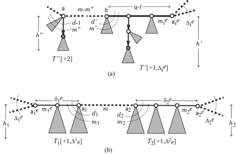
Figure 15: (a) An illustration of computing a vector $\boldsymbol{w}\in\mathrm{W}_{\mathrm{co}+1,\Delta^{e}_{i}}^{(q)}({\tt a},d,m,{\tt a}^{e}_{i},1,m^{e}_{i},h;\boldsymbol{x}^{*}_{e})$ for a base-edge $e\in E_{B}$ from the frequency vectors $\boldsymbol{w}^{\prime}=\boldsymbol{f}(T^{\prime\prime}[+1,\Delta^{e}_{i}])\in\mathrm{W}_{\mathrm{co}+1,\Delta^{e}_{i}}^{(q-1)}({\tt b},d^{\prime},m^{\prime},{\tt a}^{e}_{i},1,m^{e}_{i},h^{\prime};\boldsymbol{x}^{*}_{e})$ of a c-tree $T^{\prime}$ and $\boldsymbol{w}^{\prime\prime}=\boldsymbol{f}(T^{\prime\prime}[+2])\in\mathrm{W}_{\mathrm{co}+2}^{(0)}({\tt a},d-1,m^{\prime\prime},h^{\prime\prime};\boldsymbol{x}^{*}_{e})$ of a c-tree $T^{\prime\prime}$; (b) An illustration of computing a feasible vector pair $(\boldsymbol{w}^{1},\boldsymbol{w}^{2})$ with $\boldsymbol{w}^{i}=\boldsymbol{f}(T_{i}[+1,\Delta_{i}^{e}])\in\mathrm{W}_{\mathrm{co}+1,\Delta_{i}^{e}}^{(\delta_{i}^{e})}({\tt a}_{i},d_{i},m_{i},{\tt a}_{i}^{e},1,m_{i}^{e},h_{i};\boldsymbol{x}^{*}_{e})$, of c-trees $T_{i}$ $i=1,2$ for a base-edge $e\in E_{B}$.

6.5.5 Step 4: Generation of Frequency Vectors of Bi-rooted Core-subtrees

For each base-edge $e\in E_{B}$, each index $i=1,2$ and each possible tuple $({\tt a},d,m,h)$ with $h\in[\mathrm{ch}_{\mathrm{LB}}(e),\mathrm{ch}_{\mathrm{UB}}(e)]$, Step 4 computes the set $\mathrm{W}_{\mathrm{co}+1,\Delta^{e}_{i}}^{(q)}({\tt a},d,m,{\tt a}^{e}_{i},1,m^{e}_{i},h;x^{*}_{e})$ in the ascending order $q=1,2,\ldots,\delta^{e}_{i}$. Observe that each vector $\boldsymbol{w}\in\mathrm{W}_{\mathrm{co}+1,\Delta^{e}_{i}}^{(q)}({\tt a},d,m,{\tt a}^{e}_{i},1,m^{e}_{i},h;x^{*}_{e})$, is obtained as $\boldsymbol{w}=\boldsymbol{w}^{\prime}+\boldsymbol{w}^{\prime\prime}+\boldsymbol{1}_{\gamma^{\mathrm{co}}}$ from a combination of vectors $\boldsymbol{w}^{\prime}\in\mathrm{W}_{\mathrm{co}+1,\Delta^{e}_{i}}^{(q-1)}({\tt b},d^{\prime},m^{\prime},{\tt a}^{e}_{i},1,m^{e}_{i},h^{\prime};x^{*}_{e})$, and $\boldsymbol{w}^{\prime\prime}\in\mathrm{W}_{\mathrm{co}+2}^{(0)}({\tt a},d-1,m^{\prime\prime},h^{\prime\prime};x^{*}_{e})$ such that

$$\begin{array}[]{l}h=\max\{h^{\prime},h^{\prime\prime}\}\in[\mathrm{ch}_{\mathrm{LB}}(e),\mathrm{ch}_{\mathrm{UB}}(e)],~{}m^{\prime\prime}\leq\mathrm{val}({\tt a}_{1})-2,~{}1\leq m-m^{\prime\prime}\leq\mathrm{val}(b)-m^{\prime},\\ \boldsymbol{w}^{\prime}+\boldsymbol{w}^{\prime\prime}+\boldsymbol{1}_{\gamma^{\mathrm{co}}}\leq\boldsymbol{x}^{*}_{e}\mbox{ for }\gamma=({\tt a}d,{\tt b}\{d^{\prime}\!+\!1\},m-m^{\prime\prime})\in\Gamma_{\leq}.\end{array}$$

Figure 15(a) illustrates this process of computing a vector $\boldsymbol{w}\in\mathrm{W}_{\mathrm{co}+1,\Delta^{e}_{i}}^{(q)}({\tt a},d,m,{\tt a}^{e}_{i},1,m^{e}_{i},h;x^{*}_{e})$,

For each vector $\boldsymbol{w}\in\mathrm{W}_{\mathrm{co}+1,\Delta^{e}_{i}}^{(q)}({\tt a},d,m,{\tt a}^{e}_{i},1,m^{e}_{i},h;x^{*}_{e})$ obtained from a combination $\boldsymbol{w}^{\prime}\in\mathrm{W}_{\mathrm{co}+1,\Delta^{e}_{i}}^{(q-1)}({\tt b},$ $d^{\prime},m^{\prime},{\tt a}^{e}_{i},1,m^{e}_{i},h^{\prime};x^{*}_{e})$ and $\boldsymbol{w}^{\prime\prime}\in\mathrm{W}_{\mathrm{co}+2}^{(0)}({\tt a},d-1,m^{\prime\prime},h^{\prime\prime};x^{*}_{e})$, we construct at least one sample c-tree $T_{\boldsymbol{w}}$ from their sample nc-trees $T_{\boldsymbol{w}^{\prime}}\in\mathcal{S}_{\mathrm{co}+1,\Delta^{e}_{i}}^{(q-1)}({\tt b},d^{\prime},m^{\prime},{\tt a}^{e}_{i},1,m^{e}_{i},h^{\prime};x^{*}_{e})$ and $T_{\boldsymbol{w}^{\prime\prime}}\in\mathcal{S}_{\mathrm{co}+2}^{(0)}({\tt a},d-1,m^{\prime\prime},h^{\prime\prime};x^{*}_{e})$ and store them in a set $\mathcal{S}_{\mathrm{co}+1,\Delta^{e}_{i}}^{(q)}({\tt a},d,m,{\tt a}^{e}_{i},1,m^{e}_{i},h;x^{*}_{e})$.

6.5.6 Step 5: Enumeration of Feasible Vector Pairs

For each edge $e\in E_{B}$, a feasible vector pair is defined to be a pair of vectors $\boldsymbol{w}^{i}\in\mathrm{W}_{\mathrm{co}+1,\Delta_{i}^{e}}^{(\delta_{i}^{e})}({\tt a}_{i},d_{i},$ $m_{i},{\tt a}_{i}^{e},1,m_{i}^{e},h_{i};\boldsymbol{x}^{*}_{e})$, $i=1,2$ that satisfies

$$\max\{h_{1},h_{2}\}\in[\mathrm{ch}_{\mathrm{LB}}(e),\mathrm{ch}_{\mathrm{UB}}(e)]\mbox{ and }\boldsymbol{x}^{*}_{e}=\boldsymbol{w}^{1}+\boldsymbol{w}^{2}+\boldsymbol{1}_{\gamma}$$

for an edge-configuration $\gamma=({\tt a}_{1}\{d_{1}\!+\!1\},{\tt a}_{2}\{d_{2}\!+\!1\},m)\in\Gamma_{\leq}$ with an integer $m\in[1,\min\{3,\mathrm{val}({\tt a}_{1})-m_{1},\mathrm{val}({\tt a}_{2})-m_{2}\}]$. The second equality is equivalent with a condition that $\boldsymbol{w}^{1}$ is equal to the vector $\boldsymbol{x}^{*}_{e}-\boldsymbol{w}^{2}-\boldsymbol{1}_{\gamma}$, which we call the $\gamma$-complement of $\boldsymbol{w}^{2}$, and denote it by $\overline{\boldsymbol{w}^{2}}$. Figure 15(b) illustrates this process of computing a feasible vector pair $(\boldsymbol{w}^{1},\boldsymbol{w}^{2})$.

For each edge $e\in E_{B}$, Step 5 enumerates the set $\mathrm{W}_{\mathrm{pair}}(e)$ of all feasible vector pairs $(\boldsymbol{w}^{1},\boldsymbol{w}^{2})$. To efficiently search for a feasible pair of vectors in two sets $\mathrm{W}_{\mathrm{co}+1,\Delta_{i}^{e}}^{(\delta_{i}^{e})}({\tt a}_{i},d_{i},m_{i},{\tt a}_{i}^{e},1,m_{i}^{e},h_{i};\boldsymbol{x}^{*}_{e})$, $i=1,2$ with $\max\{h_{1},h_{2}\}\in[\mathrm{ch}_{\mathrm{LB}}(e),\mathrm{ch}_{\mathrm{UB}}(e)]$, we first compute the $\gamma$-complement vector $\overline{\boldsymbol{w}}$ of each vector $\boldsymbol{w}\in\mathrm{W}_{\mathrm{co}+1,\Delta_{2}^{e}}^{(\delta_{2}^{e})}({\tt a}_{2},d_{2},m_{2},{\tt a}_{2}^{e},1,m_{2}^{e},h_{2})$ for each an edge-configuration $\gamma=({\tt a}_{1}\{d_{1}+1\},{\tt a}_{2}\{d_{2}+1\},m)\in\Gamma$ with $m\in[1,\min\{3,\mathrm{val}({\tt a}_{1})-m_{1},\mathrm{val}({\tt a}_{2})-m_{2}\}]$, and denote by $\overline{\mathrm{W}_{\mathrm{co}}^{(\delta_{2})}}$ the set of the resulting $\gamma$-complement vectors. Observe that $(\boldsymbol{w}^{1},\boldsymbol{w}^{2})$ is a feasible vector pair if and only if $\boldsymbol{w}_{1}=\overline{\boldsymbol{w}_{2}}$. To find such pairs, we merge the sets $\mathrm{W}_{\mathrm{co}+1,\Delta_{1}^{e}}^{(\delta_{1}^{e})}({\tt a}_{1},d_{1},m_{1},{\tt a}_{1}^{e},1,m_{1}^{e},h_{1};\boldsymbol{x}^{*}_{e})$ and $\overline{\mathrm{W}_{\mathrm{co}}^{(\delta_{2})}}$ into a sorted list $L_{\gamma}$. Then each feasible vector pair $(\boldsymbol{w}^{1},\boldsymbol{w}^{2})$ appears as a consecutive pair of vectors $\boldsymbol{w}_{1}$ and $\overline{\boldsymbol{w}_{2}}$ in the list $L_{\gamma,\mu}$.

6.5.7 Step 6: Construction of Target Chemical Graphs

The task of Step 6 is to construct for each feasible vector pair $(\boldsymbol{w}^{1},\boldsymbol{w}^{2})\in\mathrm{W}_{\mathrm{pair}}(e)$, construct at least one target $e$-component $T_{(\boldsymbol{w}_{1},\boldsymbol{w}_{2})}\in\mathcal{T}_{e}$ by combining the sample c-trees $T_{i}=T_{\boldsymbol{w}^{i}}\in\mathcal{S}_{\mathrm{co}+1,\Delta_{i}^{e}}^{(\delta_{i}^{e})}({\tt a}_{i},d_{i},m_{i},{\tt a}_{i}^{e},1,m_{i}^{e},h_{i};\boldsymbol{x}^{*}_{e})$, $i=1,2$ with an edge $r_{1}(T_{1})r_{1}(T_{2})$ with a bond-multiplicity $m$, and store these target $e$-components $T_{(\boldsymbol{w}_{1},\boldsymbol{w}_{2})}$ in a set $\mathcal{S}(e)$. Figure 15(b) illustrates two sample c-trees $T_{i}$, $i=1,2$ to be combined with a new edge $e=r_{1}(T_{1})r_{1}(T_{2})$.

For each base-vertex $v\in B$ and each base-edge $e\in E_{B}$, a set $\mathcal{S}(v)$ of target $v$-components and a set $\mathcal{S}(e)$ of target $e$-components have be constructed. Let $\mathcal{C}$ be a collection obtained by choosing a target $v$-component $T_{v}\in\mathcal{S}(v)$ for each base-vertex $v\in B$ and and a target $e$-component $T_{e}\in\mathcal{S}(e)$ for each base-edge $e\in E_{B}$. Then a chemical graph $G^{*}(C)$ obtained by assembling these components is a target chemical graph to be inferred in Stage 5. The number of chemical graphs $G^{*}(C)$ in this manner is

$$\prod_{v\in V_{B}}|\mathcal{S}(v)|\times\prod_{e\in E_{B}}|\mathcal{S}(e)|,$$

where we ignore a possible automorphism over the resulting graphs.

For a base-edge $e\in E_{B}$ with a relatively large instance size $\delta^{e}_{2}$, the number $|\mathrm{W}_{\mathrm{pair}}(e)|$ of feasible vector pairs in Step 5 still can be very large. In fact, the size $|\mathrm{W}|$ of a vector set $\mathrm{W}$ to be computed in Steps 2 to 4 can also be considerably large during an execution of the algorithm. For such a case, we impose a time limitation on the running time for computing $\mathrm{W}$ and a memory limitation on the number of vectors stored in a vector set $\mathrm{W}$. With these limitations, we can compute only a limited subset $\widehat{\mathrm{W}}$ of each vector set $\mathrm{W}$ in Steps 2 to 4. Even with such a subset $\widehat{\mathrm{W}}$, we still can find a large size of a subset $\widehat{\mathrm{W}}_{\mathrm{pair}}(e)$ of $\mathrm{W}_{\mathrm{pair}}(e)$ in Step 5.

Our algorithm also can deliver a lower bound on the number $|\mathcal{T}_{\mathrm{t}}(\boldsymbol{x}^{*}_{\mathrm{t}})|$, $\mathrm{t}\in V_{B}\cup E_{B}$ of all target components in the following way. In Step 1, we also compute the number $t(\boldsymbol{w})$ of rooted trees $T\in\mathcal{T}^{(0)}$ in (i)-(iii). In Steps 2, 3 and 4, when a vector $\boldsymbol{w}$ is constructed from two vectors $\boldsymbol{w}^{\prime}$ and $\boldsymbol{w}^{\prime\prime}$, we iteratively compute the number $t(\boldsymbol{w})$ of all trees $T$ such that $\boldsymbol{w}$ is the frequency vector of a fictitious tree of $T$ by $t(\boldsymbol{w}):=t(\boldsymbol{w}^{\prime})\times t(\boldsymbol{w}^{\prime\prime})$. In Step 5, when a feasible vector pair $(\boldsymbol{w}^{1},\boldsymbol{w}^{2})\in\mathrm{W}_{\mathrm{pair}}(e)$ is obtained for a base-edge $e\in E_{B}$, we know that the number of the corresponding target $e$-components is $t(\boldsymbol{w}^{1})\times t(\boldsymbol{w}^{2})$. Possibly we compute a subset $\widehat{\mathrm{W}}_{\mathrm{pair}}(e)$ of $\mathrm{W}_{\mathrm{pair}}$ in Step 4. Then $(1/2)\sum_{(\boldsymbol{w}^{1},\boldsymbol{w}^{2})\in\widehat{\mathrm{W}}_{\mathrm{pair}}}t(\boldsymbol{w}^{1})\times t(\boldsymbol{w}^{2})$ gives a lower bound on the number $|\mathcal{T}_{e}|$ of target $e$-components, where we divided by 2 since an axially symmetric target $e$-component can correspond to two vector pairs in $\mathrm{W}_{\mathrm{pair}}(e)$. A lower bound on the number $|\mathcal{T}_{v}|$ of target $v$-components for a base-vertex $v\in V_{B}$ can be obtained in a similar way.

6.6 Choosing a Path-partition

This section describes how to apply our new algorithm for generating chemical isomers in Stage 4 after we obtain a chemical ${\rho}$-lean cyclic graph $G^{\dagger}$.

Let $(\sigma_{\mathrm{co}},\sigma_{\mathrm{nc}},\sigma_{\mathrm{\alpha\beta}})$ be a specification of substructures and $G^{\dagger}\in\mathcal{G}(\sigma_{\mathrm{co}},\sigma_{\mathrm{nc}},\sigma_{\mathrm{\alpha\beta}})$ be an $(\sigma_{\mathrm{co}},\sigma_{\mathrm{nc}},\sigma_{\mathrm{\alpha\beta}})$-extension, where we assume that the minimum $\sigma_{\mathrm{co}}$-extension $C_{\min}\in\mathcal{C}(\sigma_{\mathrm{co}})$ is a simple connected graph with the minimum degree at least 2. Let $C^{\dagger}=(V^{\mathrm{co}},E^{\mathrm{co}})$ denote the core of $\mathrm{Cr}(G^{\dagger})$ and $E_{0}$ denote the set of edges $e\in E_{(0/1)}$ that are removed in the construction of $C^{\dagger}$ from the seed graph $G_{\mathrm{C}}$.

To generate chemical ${\rho}$-lean cyclic graphs $G^{*}\in\mathcal{G}(\sigma_{\mathrm{co}},\sigma_{\mathrm{nc}},\sigma_{\mathrm{\alpha\beta}})$ by our new algorithm, we first choose a path-partition $\mathcal{P}=\{P_{1},P_{2},\ldots,P_{p}\}$ of the core $C^{\dagger}$. Recall that the base-graph $G_{B}=(V_{B},E_{B}=\{e_{1},e_{2},\ldots,e_{p}\})$ is determined by the partition $\mathcal{P}$ so that each edge $e_{j}\in E_{B}$ directly joins the end-vertices of each path $P_{j}\in\mathcal{P}$ and $V_{B}$ is the set of end-vertices of paths in $\mathcal{P}$. We choose a path-partition $\mathcal{P}=\{P_{1},P_{2},\ldots,P_{p}\}$ so that the next condition is satisfied.

$$V_{B}=V_{\mathrm{C}},~{}E_{B}=E_{\mathrm{C}}\setminus E_{0};$$

i.e., each edge $e_{i}\in E_{B}$ corresponds to an edge $a_{i}\in E_{\mathrm{C}}\setminus E_{0}$.

We next set a specification $\sigma_{\mathrm{ch}}$ to be a set of the lower and upper bound functions $\mathrm{ch}_{\mathrm{LB}},\mathrm{ch}_{\mathrm{UB}}:V_{\mathrm{C}}\cup E_{\mathrm{C}}\to\mathbb{Z}_{+}$ for the set $V_{B}=V_{\mathrm{C}}$ of vertices and the set $E_{B}=E_{\mathrm{C}}\setminus E_{0}$ of edges. Observe that any $(\mathcal{P},\sigma_{\mathrm{ch}})$-isomer $G^{*}$ of $\mathcal{G}^{\dagger}$ is a $(\sigma_{\mathrm{co}},\sigma_{\mathrm{nc}},\sigma_{\mathrm{\alpha\beta}})$-extension, since the assignment of elements of $\Lambda$ to the base-vertices in $V_{B}$ remains unchanged among all $(\mathcal{P},\sigma_{\mathrm{ch}})$-isomer of $\mathcal{G}^{\dagger}$. The converse is not true in general; i.e., there may be a $(\sigma_{\mathrm{co}},\sigma_{\mathrm{nc}},\sigma_{\mathrm{\alpha\beta}})$-extension $G$ that is not a $(\mathcal{P},\sigma_{\mathrm{ch}})$-isomer of $\mathcal{G}^{\dagger}$.

In Stage 5, we run our new algorithm for generating $(\mathcal{P},\sigma_{\mathrm{ch}})$-isomers $G^{*}$ of $\mathcal{G}^{\dagger}$.

We remark that when lower and upper bound functions $\mathrm{ch}_{\mathrm{LB}}$ and $\mathrm{ch}_{\mathrm{UB}}$ in a core specification $\sigma_{\mathrm{co}}$ are uniform overall vertices or edges, we can choose a path-partition $\mathcal{P}$ in a more flexible way. In this case, we can apply our algorithm if a path-partition $\mathcal{P}$ satisfies

$$V_{\mathrm{C}}^{*}\cup V_{3}^{\mathrm{co}}\subseteq V_{B}$$

for the set $V_{3}^{\mathrm{co}}$ of core-vertices $v\in V^{\mathrm{co}}$ of degree at least 3, i.e., $\deg_{C^{\dagger}}(v)\geq 3$. We can choose a path in $\mathcal{P}$ so that it ends with a core-vertex $v\in V^{\mathrm{co}}\setminus(V_{\mathrm{C}}^{*}\cup V_{3})$ of degree 2, i.e., $\deg_{C^{\dagger}}(v)=2$.

6.7 A Possible Extension to the General Graphs

When a given chemical graph $G^{\dagger}$ is not a ${\rho}$-lean cyclic graph, we can extend the definition of the chemical graph isomorphism in a flexible way. Suppose that $G^{\dagger}$ is an acyclic graph. We first choose a vertex $r$ as the root of tree $G^{\dagger}$, where $r$ is not necessarily a graph-theoretically designated vertex such as a center or a centroid. For a branch-parameter ${\rho}$ such as ${\rho}=2$, find the set $V_{\mathrm{br}}$ of all ${\rho}$-branches of the tree. We set $V_{B}:=V_{\mathrm{br}}\cup\{r\}$ to be a set of base-vertices and $\mathcal{P}=\{P_{1},\ldots,P_{p}\}$ denote the collection of paths with end-vertices of base-vertices in $V_{B}$ and no internal vertices from $V_{B}$. For each path $P_{u,v}\in\mathcal{P}$ between two base-vartices $u,v\in V_{B}$, prepare a base-edge $e=uv$ and let $E_{B}$ denote the set of the resulting base-edges. Then the base-graph $G_{B}=(V_{B},E_{B})$ in this case is a tree. Based on $G_{B}$, we can define the vertex and edge components of $G^{\dagger}$ in a similar way, and can generate target $v$-components $T_{v}$, $v\in V_{B}$ and target $e$-components $T_{e}$, $e\in E_{B}$, each of them independently, by our algorithm with a slight modification or the algorithm for trees $T$ with $\mathrm{bl}_{\rho}(T)=2$ due to Azam et al. [4].

Now consider the case where $G^{\dagger}$ is cyclic but not ${\rho}$-lean. In this case, some tree $T$ rooted at a core-vertex may contain more than one leaf ${\rho}$-branch. Let $\mathcal{T}_{\mathrm{br}}$ denote the set of all these rooted trees, and let $V_{\mathrm{br}}$ denote the set of all ${\rho}$-branches of the trees in $\mathcal{T}_{\mathrm{br}}$. Let $V^{\mathrm{co}}_{\mathrm{br}}$ denote the set of core-vertices $v$ at which some tree $T_{v}\in\mathcal{T}_{\mathrm{br}}$ is rooted. We find a path-partition $\mathcal{P}^{\mathrm{co}}$ of the core $\mathrm{Cr}(G^{\dagger})$ so that each vertex in $V^{\mathrm{co}}_{\mathrm{br}}$ is used as an end-vertex of some path $P\in\mathcal{P}^{\mathrm{co}}$. For the trees in $\mathcal{T}_{\mathrm{br}}$, we find a path-partition $\mathcal{P}^{\mathrm{nc}}$ with paths between two ${\rho}$-branches in $V_{\mathrm{br}}$ in an analogous way of the above tree case. Finally set $\mathcal{P}:=\mathcal{P}^{\mathrm{co}}\cup\mathcal{P}^{\mathrm{nc}}$ and define the base-graph $G_{B}=(V_{B},E_{B})$ based on $\mathcal{P}$. We see that target $v$-components $T_{v}$, $v\in V_{B}$ and target $e$-components $T_{e}$, $e\in E_{B}$ can be generated by our algorithm with a slight modification.

7 Concluding Remarks

In this paper, we employed the new mechanism of utilizing a target chemical graph $G^{\dagger}$ obtained in Stage 4 of the framework for inverse QSAR/QSPR to generate a larger number of target graphs $G^{*}$ in Stage 5. We showed that a family of graphs $G^{*}$ that are chemically isomorphic to $G^{\dagger}$ can be obtained by the dynamic programming algorithm designed in Section 6. Based on the new mechanism of Stage 5, we proposed a target specification on a seed graph as a flexible way of specifying a family of target chemical graphs. With this specification, we can realize requirements on partial topological substructure of the core of graphs and partial assignment of chemical elements and bond-multiplicity within the framework for inverse QSAR/QSPR by ANNs and MILPs.

The current topological specification proposed in this paper does not allow to fix part of the non-core structure of a graph. We remark that it is not technically difficult to extend the MILP formulation in Section 5 and the algorithm for computing chemical isomers in Section 6 so that a more general specification for such a case can be handled.

Appendix A All Constraints in an MILP Formulation for Chemical Cyclic Graphs

We define a standard encoding of a finite set $A$ of elements to be a bijection $\sigma:A\to[1,|A|]$, where we denote by $[A]$ the set $[1,|A|]$ of integers and by $[{\tt e}]$ the encoded element $\sigma({\tt e})$. Let $\epsilon$ denote null, a fictitious chemical element that does not belong to any set of chemical elements, chemical symbols, adjacency-configurations and edge-configurations in the following formulation. Given a finite set $A$, let $A_{\epsilon}$ denote the set $A\cup\{\epsilon\}$ and define a standard encoding of $A_{\epsilon}$ to be a bijection $\sigma:A\to[0,|A|]$ such that $\sigma(\epsilon)=0$, where we denote by $[A_{\epsilon}]$ the set $[0,|A|]$ of integers and by $[{\tt e}]$ the encoded element $\sigma({\tt e})$, where $[\epsilon]=0$.

We choose a branch-parameter ${\rho}$ and subsets $\Lambda^{\mathrm{co}},\Lambda^{\mathrm{nc}}\subseteq\Lambda$ of chemical elements, subsets $\Lambda_{\mathrm{dg}}^{\mathrm{co}}\subseteq\Lambda^{\mathrm{co}}\times[2,4]$ and $\Lambda_{\mathrm{dg}}^{\mathrm{nc}}\subseteq\Lambda^{\mathrm{nc}}\times[1,4]$ of chemical symbols, subsets $\Gamma^{\mathrm{co}}\subseteq\Gamma_{<}(\Lambda_{\mathrm{dg}}^{\mathrm{co}})\cup\Gamma_{=}(\Lambda_{\mathrm{dg}}^{\mathrm{co}})$ and $\Gamma^{\mathrm{in}},\Gamma^{\mathrm{ex}}\subseteq\Gamma(\Lambda_{\mathrm{dg}}^{\mathrm{nc}})$ of edge-configurations.

Let $(\sigma_{\mathrm{co}},\sigma_{\mathrm{nc}},\sigma_{\mathrm{\alpha\beta}})$ be a specification, and let $G$ be a chemical ${\rho}$-lean graph in $\mathcal{G}(\sigma_{\mathrm{co}},\sigma_{\mathrm{nc}},\sigma_{\mathrm{\alpha\beta}})$.

A.1 Selecting Core-vertices and Core-edges

Recall that

$$\begin{array}[]{ll}E_{(=1)}=\{e\in E_{\mathrm{C}}\mid\ell_{\mathrm{LB}}(e)=\ell_{\mathrm{UB}}(e)=1\};&E_{(0/1)}=\{e\in E_{\mathrm{C}}\mid\ell_{\mathrm{LB}}(e)=0,\ell_{\mathrm{UB}}(e)=1\};\\ E_{(\geq 1)}=\{e\in E_{\mathrm{C}}\mid\ell_{\mathrm{LB}}(e)=1,\ell_{\mathrm{UB}}(e)\geq 2\};&E_{(\geq 2)}=\{e\in E_{\mathrm{C}}\mid\ell_{\mathrm{LB}}(e)\geq 2\};\end{array}$$

1. Every edge $a_{i}\in E_{(=1)}$ is included in $G$;

2. Each edge $a_{i}\in E_{(0/1)}$ is included in $G$ if necessary;

3. For each edge $a_{i}\in E_{(\geq 2)}$, edge $a_{i}$ is not included in $G$ and instead a path

   $$P_{i}=({v^{\mathrm{C}}}_{\mathrm{tail}^{\mathrm{C}}(i)},{v^{\mathrm{T}}}_{j-1,0},{v^{\mathrm{T}}}_{j,0},\ldots,{v^{\mathrm{T}}}_{j+t,0},{v^{\mathrm{C}}}_{\mathrm{head}^{\mathrm{C}}(i)})$$

   of length at least 2 from vertex ${v^{\mathrm{C}}}_{\mathrm{tail}^{\mathrm{C}}(i),0}$ to vertex ${v^{\mathrm{C}}}_{\mathrm{head}^{\mathrm{C}}(i),0}$ visiting some core-vertices in $V_{\mathrm{T}}$ is constructed in $G$; and

4. For each edge $a_{i}\in E_{(\geq 1)}$, either edge $a_{i}$ is directly used in $G$ or the above path $P_{i}$ of length at least 2 is constructed in $G$.

Let ${t_{\mathrm{C}}}\triangleq|V_{\mathrm{C}}|$ and denote $V_{\mathrm{C}}$ by $\{{v^{\mathrm{C}}}_{i,0}\mid i\in[1,{t_{\mathrm{C}}}]\}$. Regard the seed graph $G_{\mathrm{C}}$ as a digraph such that each edge $a_{i}$ with end-vertices ${v^{\mathrm{C}}}_{j,0}$ and ${v^{\mathrm{C}}}_{j^{\prime},0}$ is directed from ${v^{\mathrm{C}}}_{j,0}$ to ${v^{\mathrm{C}}}_{j^{\prime},0}$ when $j<j^{\prime}$. For each directed edge $a_{i}\in E_{\mathrm{C}}$, let $\mathrm{head}^{\mathrm{C}}(i)$ and $\mathrm{tail}^{\mathrm{C}}(i)$ denote the head and tail of ${e^{\mathrm{C}}}(i)$; i.e., $a_{i}=({v^{\mathrm{C}}}_{\mathrm{tail}^{\mathrm{C}}(i),0},{v^{\mathrm{C}}}_{\mathrm{head}^{\mathrm{C}}(i),0})$.

Assume that $E_{\mathrm{C}}=\{a_{i}\mid i\in[1,m_{\mathrm{C}}]\}$, $E_{(\geq 2)}=\{a_{k}\mid k\in[1,p]\}$, $E_{(\geq 2)}=\{a_{k}\mid k\in[p+1,q]\}$, $E_{(0/1)}=\{a_{i}\mid i\in[q+1,t]\}$ and $E_{(=1)}=\{a_{i}\mid i\in[t+1,m_{\mathrm{C}}]\}$ for integers $p,q$ and $t$. Define

$${k_{\mathrm{C}}}\triangleq|E_{(\geq 2)}\cup E_{(\geq 1)}|,~{}~{}\widetilde{{k_{\mathrm{C}}}}\triangleq|E_{(\geq 2)}|.$$

To control construction of such a path $P_{i}$ for each edge $a_{k}\in E_{(\geq 2)}\cup E_{(\geq 1)}$, we regard the index $k\in[1,{k_{\mathrm{C}}}]$ of each edge $a_{k}\in E_{(\geq 2)}\cup E_{(\geq 1)}$ as the “color” of the edge. To introduce necessary linear constraints that can construct such a path $P_{k}$ properly in our MILP, we assign the color $k$ to the vertices ${v^{\mathrm{T}}}_{j-1,0},{v^{\mathrm{T}}}_{j,0},\ldots,$ ${v^{\mathrm{T}}}_{j+t,0}$ in $V_{\mathrm{T}}$ when the above path $P_{k}$ is used in $G$.

For each index $s\in[1,{t_{\mathrm{C}}}]$, let $E_{(=1)}^{+}(s)$ (resp., $E_{(=1)}^{-}(s)$) denote the set of edges $e\in E_{(=1)}$ such that the tail (resp., head) of $a_{i}$ is ${v^{\mathrm{C}}}_{s,0}$. Similarly for $E_{(0/1)}^{+}(s)$, $E_{(0/1)}^{-}(s)$, $E_{(\geq 1)}^{+}(s)$, $E_{(\geq 1)}^{-}(s)$, $E_{(\geq 2)}^{+}(s)$ and $E_{(\geq 2)}^{-}(s)$.

Let $I_{(=1)}$ denote the set of indices $i$ of edges $a_{i}\in E_{(=1)}$. Similarly for $I_{(0/1)}$, $I_{(\geq 1)}$, $I_{(\geq 2)}$, $I_{(=1)}^{+}(s)$, $I_{(=1)}^{-}(s)$, $I_{(0/1)}^{+}(s)$, $I_{(0/1)}^{-}(s)$, $I_{(\geq 1)}^{+}(s)$, $I_{(\geq 1)}^{-}(s)$, $I_{(\geq 2)}^{+}(s)$ and $I_{(\geq 2)}^{-}(s)$. Note that $[1,{k_{\mathrm{C}}}]=I_{(\geq 2)}\cup I_{(\geq 1)}$ and $[\widetilde{{k_{\mathrm{C}}}}+1,m_{\mathrm{C}}]=I_{(\geq 1)}\cup I_{(0/1)}\cup I_{(=1)}$.

constants:
   ${t_{\mathrm{C}}}=|V_{\mathrm{C}}|$, $\widetilde{{k_{\mathrm{C}}}}=|E_{(\geq 2)}|$, ${k_{\mathrm{C}}}=|E_{(\geq 2)}\cup E_{(\geq 1)}|$, ${t_{\mathrm{T}}}=\mathrm{cs}_{\mathrm{UB}}-|V_{\mathrm{C}}|$, $m_{\mathrm{C}}=|E_{\mathrm{C}}|$,
      where $a_{i}\in E_{\mathrm{C}}\setminus(E_{(\geq 2)}\cup E_{(\geq 1)})$, $i\in[{k_{\mathrm{C}}}+1,m_{\mathrm{C}}]$;

constants for core specification $\sigma_{\mathrm{co}}$:
   $\mathrm{cs}_{\mathrm{LB}},\mathrm{cs}_{\mathrm{UB}}\in[2,n^{*}]$; lower and upper bounds on $\mathrm{cs}(G)$;
   $\ell_{\mathrm{LB}}(k),\ell_{\mathrm{UB}}(k)\in[1,{t_{\mathrm{T}}}]$, $k\in[1,{k_{\mathrm{C}}}]$: lower and upper bounds on the length of path $P_{k}$;

constants for core specification $\sigma_{\mathrm{nc}}$:
   $\mathrm{bl}_{\mathrm{LB}}(i),\mathrm{bl}_{\mathrm{UB}}(i)\in[0,1]$, $i\in[1,{t_{\mathrm{T}}}]$: lower and upper bounds on $\mathrm{bl}_{\rho}(T_{i})$ of the tree rooted
      at a vertex ${v^{\mathrm{C}}}_{i,0}$;

variables:
   ${e^{\mathrm{C}}}(i)\in[0,1]$, $i\in[1,m_{\mathrm{C}}]$: ${e^{\mathrm{C}}}(i)$ represents edge $a_{i}\in E_{\mathrm{C}}$, $i\in[1,m_{\mathrm{C}}]$
        (${e^{\mathrm{C}}}(i)=1$, $i\in I_{(=1)}$; ${e^{\mathrm{C}}}(i)=0$, $i\in I_{(\geq 2)}$)
        (${e^{\mathrm{C}}}(i)=1$ $\Leftrightarrow$ edge $a_{i}$ is used in $G$);
   ${v^{\mathrm{T}}}(i,0)\in[0,1]$, $i\in[1,{t_{\mathrm{T}}}]$:
       ${v^{\mathrm{T}}}(i,0)=1$ $\Leftrightarrow$ vertex ${v^{\mathrm{T}}}_{i,0}$ is used in $G$;
   ${e^{\mathrm{T}}}(i)\in[0,1]$, $i\in[1,{t_{\mathrm{T}}}+1]$: ${e^{\mathrm{T}}}(i)$ represents edge ${e^{\mathrm{T}}}_{i}=({v^{\mathrm{T}}}_{i-1,0},{v^{\mathrm{T}}}_{i,0})\in E_{\mathrm{T}}$,
       where ${e^{\mathrm{T}}}_{1}$ and ${e^{\mathrm{T}}}_{{t_{\mathrm{T}}}+1}$ are fictitious edges (${e^{\mathrm{T}}}(i)=1$ $\Leftrightarrow$ edge ${e^{\mathrm{T}}}_{i}$ is used in $G$);
   ${\chi^{\mathrm{T}}}(i)\in[0,{k_{\mathrm{C}}}]$, $i\in[1,{t_{\mathrm{T}}}]$: ${\chi^{\mathrm{T}}}(i)$ represents the color assigned to core-vertex ${v^{\mathrm{T}}}_{i,0}$
       (${\chi^{\mathrm{T}}}(i)=k>0$ $\Leftrightarrow$ vertex ${v^{\mathrm{T}}}_{i,0}$ is assigned color $k$;
       ${\chi^{\mathrm{T}}}(i)=0$ means that vertex ${v^{\mathrm{T}}}_{i,0}$ is not used in $G$);
   $\mathrm{clr}^{\mathrm{T}}(k)\in[\ell_{\mathrm{LB}}(k)-1,\ell_{\mathrm{UB}}(k)-1]$, $k\in[1,{k_{\mathrm{C}}}]$ $\mathrm{clr}^{\mathrm{T}}(0)\in[0,{t_{\mathrm{T}}}]$: the number of vertices ${v^{\mathrm{T}}}_{i,0}\in V_{\mathrm{T}}$
       with color $c$ (the range $[\ell_{\mathrm{LB}}(c)-1,\ell_{\mathrm{UB}}(c)-1]$ expresses a constraint in $\sigma_{\mathrm{co}}$);
   $\delta_{\mathrm{\chi}}^{\mathrm{T}}(k)\in[0,1]$, $k\in[0,{k_{\mathrm{C}}}]$: $\delta_{\mathrm{\chi}}^{\mathrm{T}}(k)=1$ $\Leftrightarrow$ ${\chi^{\mathrm{T}}}(i)=k$ for some $i\in[1,{t_{\mathrm{T}}}]$;
   ${\chi^{\mathrm{T}}}(i,k)\in[0,1]$, $i\in[1,{t_{\mathrm{T}}}]$, $k\in[0,{k_{\mathrm{C}}}]$ (${\chi^{\mathrm{T}}}(i,k)=1$ $\Leftrightarrow$ ${\chi^{\mathrm{T}}}(i)=k$);
   ${\widetilde{\deg}_{\mathrm{C}}}^{+}(i)\in[0,4]$, $i\in[1,{t_{\mathrm{C}}}]$: the out-degree of vertex ${v^{\mathrm{C}}}_{i,0}$ with the used edges ${e^{\mathrm{C}}}$ in $E_{\mathrm{C}}$;
   ${\widetilde{\deg}_{\mathrm{C}}}^{-}(i)\in[0,4]$, $i\in[1,{t_{\mathrm{C}}}]$: the in-degree of vertex ${v^{\mathrm{C}}}_{i,0}$ with the used edges ${e^{\mathrm{C}}}$ in $E_{\mathrm{C}}$;

variables for specification $\sigma_{\mathrm{co}}$:
   $\mathrm{cs}\in[\mathrm{cs}_{\mathrm{LB}},\mathrm{cs}_{\mathrm{UB}}]$: the core size (the range $[\mathrm{cs}_{\mathrm{LB}},\mathrm{cs}_{\mathrm{UB}}]$ expresses a constraint in $\sigma_{\mathrm{co}}$);

constraints:

$${e^{\mathrm{C}}}(i)=1,~{}~{}~{}i\in I_{(=1)},$$ (3)

$${e^{\mathrm{C}}}(i)=0,~{}~{}\mathrm{clr}^{\mathrm{T}}(i)\geq 1,~{}~{}~{}i\in I_{(\geq 2)},$$ (4)

$${e^{\mathrm{C}}}(i)+\mathrm{clr}^{\mathrm{T}}(i)\geq 1,~{}~{}~{}~{}~{}\mathrm{clr}^{\mathrm{T}}(i)\leq{t_{\mathrm{T}}}\cdot(1-{e^{\mathrm{C}}}(i)),~{}~{}~{}i\in I_{(\geq 1)},$$ (5)

$$\sum_{c\in I_{(\geq 1)}^{-}(i)\cup I_{(0/1)}^{-}(i)\cup I_{(=1)}^{-}(i)}\!\!\!\!\!\!{e^{\mathrm{C}}}(c)={\widetilde{\deg}_{\mathrm{C}}}^{-}(i),~{}~{}\sum_{c\in I_{(\geq 1)}^{+}(i)\cup I_{(0/1)}^{+}(i)\cup I_{(=1)}^{+}(i)}\!\!\!\!\!\!{e^{\mathrm{C}}}(c)={\widetilde{\deg}_{\mathrm{C}}}^{+}(i), i\in[1,{t_{\mathrm{C}}}],$$ (6)

$${\chi^{\mathrm{T}}}(i,0)=1-{v^{\mathrm{T}}}(i,0),~{}~{}~{}\sum_{k\in[0,{k_{\mathrm{C}}}]}{\chi^{\mathrm{T}}}(i,k)=1,~{}~{}~{}\sum_{k\in[0,{k_{\mathrm{C}}}]}k\cdot{\chi^{\mathrm{T}}}(i,k)={\chi^{\mathrm{T}}}(i), i\in[1,{t_{\mathrm{T}}}],$$ (7)

$$\sum_{i\in[1,{t_{\mathrm{T}}}]}{\chi^{\mathrm{T}}}(i,k)=\mathrm{clr}^{\mathrm{T}}(k),~{}~{}{t_{\mathrm{T}}}\cdot\delta_{\mathrm{\chi}}^{\mathrm{T}}(k)\geq\sum_{i\in[1,{t_{\mathrm{T}}}]}{\chi^{\mathrm{T}}}(i,k)\geq\delta_{\mathrm{\chi}}^{\mathrm{T}}(k), k\in[0,{k_{\mathrm{C}}}],$$ (8)

$${v^{\mathrm{T}}}(i-1,0)\geq{v^{\mathrm{T}}}(i,0),$$

$${k_{\mathrm{C}}}\cdot({v^{\mathrm{T}}}(i-1,0)-{e^{\mathrm{T}}}(i))\geq{\chi^{\mathrm{T}}}(i-1)-{\chi^{\mathrm{T}}}(i)\geq{v^{\mathrm{T}}}(i-1,0)-{e^{\mathrm{T}}}(i), i\in[2,{t_{\mathrm{T}}}],$$ (9)

$${t_{\mathrm{C}}}+\sum_{i\in[1,{t_{\mathrm{T}}}]}{v^{\mathrm{T}}}(i,0)=\mathrm{cs}.$$ (10)

A.2 Constraints for Including Internal Vertices and Edges

Define the set of colors for the vertex set $\{u_{i}\mid i\in[1,\widetilde{{t_{\mathrm{C}}}}]\}\cup V_{\mathrm{T}}$ to be $[1,{c_{\mathrm{F}}}]$ with

$${c_{\mathrm{F}}}\triangleq\widetilde{{t_{\mathrm{C}}}}+{t_{\mathrm{T}}}=|\{u_{i}\mid i\in[1,\widetilde{{t_{\mathrm{C}}}}]\}\cup V_{\mathrm{T}}|.$$

Let each core-vertex ${v^{\mathrm{C}}}_{i,0}$, $i\in[1,\widetilde{{t_{\mathrm{C}}}}]$ (resp., ${v^{\mathrm{T}}}_{i,0}\in V_{\mathrm{T}}$) correspond to a color $i\in[1,{c_{\mathrm{F}}}]$ (resp., $i+\widetilde{{t_{\mathrm{C}}}}\in[1,{c_{\mathrm{F}}}]$). Let $\mathrm{tail}^{\mathrm{F}}(i):=i$ for each color $i\in[1,\widetilde{{t_{\mathrm{C}}}}]$ and $\mathrm{tail}^{\mathrm{F}}(i):=i-{t_{\mathrm{C}}}$ for each color $i\in[\widetilde{{t_{\mathrm{C}}}}+1,{c_{\mathrm{F}}}]$. When a path $P=(u,{v^{\mathrm{F}}}_{j,0},{v^{\mathrm{F}}}_{j+1,0},\ldots,{v^{\mathrm{F}}}_{j+t,0})$ from a vertex $u\in V_{\mathrm{C}}\cup V_{\mathrm{T}}$ is used in $G$, we assign the color $i\in[1,{c_{\mathrm{F}}}]$ of the vertex $u$ to the vertices ${v^{\mathrm{F}}}_{j,0},{v^{\mathrm{F}}}_{j+1,0},\ldots,{v^{\mathrm{F}}}_{j+t,0}$ in $V_{\mathrm{F}}$.

constants:
   ${c_{\mathrm{F}}}$: the maximum number of different colors assigned to the vertices in $V_{\mathrm{F}}$;
constants for non-core specification $\sigma_{\mathrm{nc}}$:
   $\mathrm{bl}_{\mathrm{LB}}(i)\in[0,1]$, $i\in[1,\widetilde{{t_{\mathrm{C}}}}]$: a lower bound on the number of leaf ${\rho}$-branches
       in the tree rooted at $u_{i}\in V_{\mathrm{C}}$;
   $\mathrm{bl}_{\mathrm{LB}}(k),\mathrm{bl}_{\mathrm{UB}}(k)\in[0,\ell_{\mathrm{UB}}(k)-1]$, $k\in[1,{k_{\mathrm{C}}}]=I_{(\geq 2)}\cup I_{(\geq 1)}$: lower and upper bounds on the sum
      of $\mathrm{bl}_{\rho}(T)$ of the trees rooted at internal vertices of a path $P_{k}$ for an edge $a_{k}\in E_{(\geq 1)}\cup E_{(\geq 2)}$;

variables:
    $\mathrm{bl}_{G}\in[0,\max[\max\{\mathrm{bl}_{\mathrm{UB}}(v)\mid v\in V_{\mathrm{C}}\},\max\{\mathrm{bl}_{\mathrm{UB}}(e)\mid e\in E_{\mathrm{C}}\}]$: $\mathrm{bl}_{\rho}(G)$;
   ${v^{\mathrm{F}}}(i,0)\in[0,1]$, $i\in[1,{t_{\mathrm{F}}}]$:
       ${v^{\mathrm{F}}}(i,0)=1$ $\Leftrightarrow$ vertex ${v^{\mathrm{F}}}_{i,0}$ is used in $G$;
   ${e^{\mathrm{F}}}(i)\in[0,1]$, $i\in[1,{t_{\mathrm{F}}}+1]$: ${e^{\mathrm{F}}}(i)$ represents edge ${e^{\mathrm{F}}}_{i}={v^{\mathrm{F}}}_{i-1,0}{v^{\mathrm{F}}}_{t,0}$,
       where ${e^{\mathrm{F}}}_{1}$ and ${e^{\mathrm{F}}}_{{t_{\mathrm{F}}}+1}$ are fictitious edges (${e^{\mathrm{F}}}(i)=1$ $\Leftrightarrow$ edge ${e^{\mathrm{F}}}_{i}$ is used in $G$);
   ${\chi^{\mathrm{F}}}(i)\in[0,{c_{\mathrm{F}}}]$, $i\in[1,{t_{\mathrm{F}}}]$: ${\chi^{\mathrm{F}}}(i)$ represents the color assigned to non-core-vertex ${v^{\mathrm{F}}}_{i,0}$
       (${\chi^{\mathrm{F}}}(i)=c$ $\Leftrightarrow$ vertex ${v^{\mathrm{F}}}_{i,0}$ is assigned color $c$);
   $\mathrm{clr}^{\mathrm{F}}(c)\in[0,{t_{\mathrm{F}}}]$, $c\in[0,{c_{\mathrm{F}}}]$: the number of vertices ${v^{\mathrm{F}}}_{i,0}$ with color $c$;
   $\delta_{\mathrm{\chi}}^{\mathrm{F}}(c)\in[\mathrm{bl}_{\mathrm{LB}}(c),1]$, $c\in[1,\widetilde{{t_{\mathrm{C}}}}]$: $\delta_{\mathrm{\chi}}^{\mathrm{F}}(c)=1$ $\Leftrightarrow$ ${\chi^{\mathrm{F}}}(i)=c$ for some $i\in[1,{t_{\mathrm{F}}}]$;
   $\delta_{\mathrm{\chi}}^{\mathrm{F}}(c)\in[0,1]$, $c\in[\widetilde{{t_{\mathrm{C}}}}+1,{c_{\mathrm{F}}}]$: $\delta_{\mathrm{\chi}}^{\mathrm{F}}(c)=1$ $\Leftrightarrow$ ${\chi^{\mathrm{F}}}(i)=c$ for some $i\in[1,{t_{\mathrm{F}}}]$;
   ${\chi^{\mathrm{F}}}(i,c)\in[0,1]$, $i\in[1,{t_{\mathrm{F}}}]$, $c\in[0,{c_{\mathrm{F}}}]$: ${\chi^{\mathrm{F}}}(i,c)=1$ $\Leftrightarrow$ ${\chi^{\mathrm{F}}}(i)=c$;
   $\sigma(c)\in[0,1]$, $c\in[0,{c_{\mathrm{F}}}]$: $\sigma(c)=1$ $\Leftrightarrow$ the ${\rho}$-pendent-tree rooted at vertex ${v^{\mathrm{C}}}_{c,0}$ $(c\leq\widetilde{{t_{\mathrm{C}}}})$
       or ${v^{\mathrm{T}}}_{c-\widetilde{{t_{\mathrm{C}}}},0}$ $(c>\widetilde{{t_{\mathrm{C}}}})$ has the core height $\mathrm{ch}_{G}$.
   $\sigma^{\mathrm{X}}(i)\in[0,1]$, $i\in[1,{t_{\mathrm{X}}}]$, $\mathrm{X}\in\{\mathrm{C,T,F}\}$: $\sigma^{\mathrm{X}}(i)=1$ $\Leftrightarrow$ the subtree of $X_{i}$ rooted
       at vertex ${v^{\mathrm{X}}}_{i,0}$ has the core height $\mathrm{ch}_{G}$.

variables for chemical specification $\sigma_{\mathrm{nc}}$:
   $\mathrm{bl}(k,i)\in[0,1]$, $k\in[1,{k_{\mathrm{C}}}]=I_{(\geq 2)}\cup I_{(\geq 1)}$, $i\in[1,{t_{\mathrm{T}}}]$: $\mathrm{bl}(k,i)=1$ $\Leftrightarrow$ path $P_{k}$ contains vertex ${v^{\mathrm{T}}}_{i,0}$
       as an internal vertex and the ${\rho}$-fringe-tree rooted at ${v^{\mathrm{T}}}_{i,0}$ contains a leaf ${\rho}$-branch;

constraints:

$${\chi^{\mathrm{F}}}(i,0)=1-{v^{\mathrm{F}}}(i,0),~{}~{}~{}\sum_{c\in[0,{c_{\mathrm{F}}}]}{\chi^{\mathrm{F}}}(i,c)=1,~{}~{}~{}\sum_{c\in[0,{c_{\mathrm{F}}}]}c\cdot{\chi^{\mathrm{F}}}(i,c)={\chi^{\mathrm{F}}}(i), i\in[1,{t_{\mathrm{F}}}],$$ (11)

$$\sum_{i\in[1,{t_{\mathrm{F}}}]}{\chi^{\mathrm{F}}}(i,c)=\mathrm{clr}^{\mathrm{F}}(c),~{}~{}~{}{t_{\mathrm{F}}}\cdot\delta_{\mathrm{\chi}}^{\mathrm{F}}(c)\geq\sum_{i\in[1,{t_{\mathrm{F}}}]}{\chi^{\mathrm{F}}}(i,c)\geq\delta_{\mathrm{\chi}}^{\mathrm{F}}(c), c\in[0,{c_{\mathrm{F}}}],$$ (12)

$${e^{\mathrm{F}}}(1)={e^{\mathrm{F}}}({t_{\mathrm{F}}}+1)=0,$$ (13)

$${v^{\mathrm{F}}}(i-1,0)\geq{v^{\mathrm{F}}}(i,0),$$

$${c_{\mathrm{F}}}\cdot({v^{\mathrm{F}}}(i-1,0)-{e^{\mathrm{F}}}(i))\geq{\chi^{\mathrm{F}}}(i-1)-{\chi^{\mathrm{F}}}(i)\geq{v^{\mathrm{F}}}(i-1,0)-{e^{\mathrm{F}}}(i), i\in[2,{t_{\mathrm{F}}}],$$ (14)

$$\sum_{c\in[1,{c_{\mathrm{F}}}]}\delta_{\mathrm{\chi}}^{\mathrm{F}}(c)=\mathrm{bl}_{G},~{}~{}\sum_{c\in[1,{c_{\mathrm{F}}}]}\sigma(c)+\sum_{i\in[1,{t_{\mathrm{X}}}],\mathrm{X}\in\{\mathrm{C,T,F}\}}\sigma^{\mathrm{X}}(i)=1,$$ (15)

$$\mathrm{bl}(k,i)\geq\delta_{\mathrm{\chi}}^{\mathrm{F}}(\widetilde{{t_{\mathrm{C}}}}+i)+{\chi^{\mathrm{T}}}(i,k)-1,~{}~{}~{}~{}~{}~{}~{}~{}k\in[1,{k_{\mathrm{C}}}],i\in[1,{t_{\mathrm{T}}}],$$ (16)

$$\sum_{k\in[1,{k_{\mathrm{C}}}],i\in[1,{t_{\mathrm{T}}}]}\mathrm{bl}(k,i)\leq\sum_{i\in[1,{t_{\mathrm{T}}}]}\delta_{\mathrm{\chi}}^{\mathrm{F}}(\widetilde{{t_{\mathrm{C}}}}+i),$$ (17)

$$\mathrm{bl}_{\mathrm{LB}}(k)\leq\sum_{i\in[1,{t_{\mathrm{T}}}]}\mathrm{bl}(k,i)\leq\mathrm{bl}_{\mathrm{UB}}(k),~{}~{}~{}~{}~{}~{}k\in[1,{k_{\mathrm{C}}}].$$ (18)

A.3 Constraints for Including Fringe-trees

We set $d_{\max}=3$ if $\mathrm{dg}^{\mathrm{nc}}_{4,\mathrm{UB}}=0$, and $d_{\max}=4$ if $\mathrm{dg}^{\mathrm{nc}}_{4,\mathrm{UB}}\geq 1$.

Since we use the proper sets $P_{\mathrm{prc}}(1,2,2)$, $P_{\mathrm{prc}}(2,2,2)$, $P_{\mathrm{prc}}(2,3,2)$ and $P_{\mathrm{prc}}(3,3,2)$ of ordered index pairs in Section 2, we observe that some vertices in the trees $T(1,2,2)$, $T(2,2,2)$, $T(1,3,2)$, $T(2,3,2)$ and $T(3,3,2)$ will not be used in any choice of subtrees. In this MILP formulation, we use the reduce trees $T^{\prime}$ illustrated in Figure 16(a)-(d).

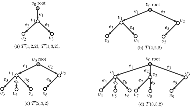
Figure 16: An illustration of reduced trees $T^{\prime}$ of rooted trees $T(a,b,c)$: (a) A reduced tree for $T(1,2,2)=T(d_{\max}-2,d_{\max}-1,{\rho})$ with $d_{\max}=3$ and ${\rho}=2$ and for $T(1,3,2)=T(d_{\max}-3,d_{\max}-1,{\rho})$ with $d_{\max}=4$ and ${\rho}=2$; (b) A reduced tree for $T(2,2,2)=T(d_{\max}-1,d_{\max}-1,{\rho})$ with $d_{\max}=3$ and ${\rho}=2$; (c) A reduced tree for $T(2,3,2)=T(d_{\max}-2,d_{\max}-1,{\rho})$ with $d_{\max}=4$ and ${\rho}=2$; (d) A reduced tree for $T(3,3,2)=T(d_{\max}-1,d_{\max}-1,{\rho})$ with $d_{\max}=4$ and ${\rho}=2$.

We introduce some notations of rooted trees in the scheme graph $\mathrm{SG}$.
   For each rooted tree $X_{i}$ such that $C_{i}=T(\Delta_{i},d_{\max}-1,{\rho})$, $T_{i}=T(d_{\max}-2,d_{\max}-1,{\rho})$ and $F_{i}=T(d_{\max}-1,d_{\max}-1,{\rho})$, $\mathrm{X}\in\{\mathrm{C,T,F}\}$,
       $\mathrm{Cld}_{\mathrm{X}}(j)$ denotes the set of the indices $h$ of children ${v^{\mathrm{X}}}_{i,h}$ of a vertex ${v^{\mathrm{X}}}_{i,j}$;
       $\mathrm{prt}_{\mathrm{X}}(j)$ denotes the index $h$ of the parent ${v^{\mathrm{X}}}_{i,h}$ of a non-root vertex ${v^{\mathrm{X}}}_{i,j}$;
       $\mathrm{Dsn}_{\mathrm{X}}(p)$ denotes the set of indices $j$ of a vertex ${v^{\mathrm{X}}}_{i,j}$ whose depth is $p$;
       $P_{\mathrm{prc,X}}$ is a proper set $P_{\mathrm{prc}}(d_{\mathrm{X}},d_{\max}-1,{\rho})$ of index pairs,
       where $d_{\mathrm{C}}=\Delta_{i}$, $d_{\mathrm{T}}=2$ and $d_{\mathrm{F}}=d_{\max}-1$;
       $j^{\mathrm{X}}_{p}$ denotes the index $j\in\mathrm{Dsn}_{\mathrm{X}}(p)$ of the vertex ${v^{\mathrm{X}}}_{i,j}$ with depth $p$ in the leftmost path
            from the root (where assume that the height of a rooted tree
            satisfying $P_{\mathrm{prc,X}}$ is given by the leftmost path from the root);

We assume that every rooted tree $T\in\mathcal{T}_{\mathrm{prc}}(d_{\max}-2,d_{\max}-1,{\rho})$ (resp., $T\in\mathcal{T}_{\mathrm{prc}}(d_{\max}-1,d_{\max}-1,{\rho})$) satisfies a property that the leftmost path (or the path that visits children with the smallest index) from the root is alway is the height $\mathrm{ht}(T)$.

To express the condition that a ${\rho}$-fringe-tree is chosen from a rooted tree $C_{i}$, $T_{i}$ or $F_{i}$, we introduce the following set of variables and constraints.

constants for non-core specification $\sigma_{\mathrm{nc}}$:
   $n_{\mathrm{LB}},n^{*}\geq\mathrm{cs}_{\mathrm{LB}}$: lower and upper bounds on $n(G)$;
   $\mathrm{ch}_{\mathrm{LB}}(i),\mathrm{ch}_{\mathrm{UB}}(i)\in[0,n^{*}]$, $i\in[1,{t_{\mathrm{T}}}]$: lower and upper bounds on $\mathrm{ht}(T_{i})$ of the tree rooted
      at a vertex ${v^{\mathrm{C}}}_{i,0}$;
   $\mathrm{ch}_{\mathrm{LB}}(k),\mathrm{ch}_{\mathrm{UB}}(k)\in[0,n^{*}]$, $k\in[1,{k_{\mathrm{C}}}]=I_{(\geq 2)}\cup I_{(\geq 1)}$: lower and upper bounds on the maximum
      height $\mathrm{ht}(T)$ of the tree $T\in\mathcal{F}(P_{k})$ of rooted at an internal vertex of a path $P_{k}$
      for an edge $a_{k}\in E_{(\geq 1)}\cup E_{(\geq 2)}$;

variables:
   $n_{G}\in[n_{\mathrm{LB}},n^{*}]$: $n(G)$;
   $\mathrm{ch}_{G}\in[0,\max[\max\{\mathrm{ch}_{\mathrm{UB}}(v)\mid v\in V_{\mathrm{C}}\},\max\{\mathrm{ch}_{\mathrm{UB}}(e)\mid e\in E_{\mathrm{C}}\}]$: $\mathrm{ch}(G)$;
   ${v^{\mathrm{T}}}(i,j)\in[0,1]$, $i\in[1,{t_{\mathrm{T}}}]$, $j\in[1,n_{\mathrm{T}}]$:
       ${v^{\mathrm{T}}}(i,j)=1$ $\Leftrightarrow$ vertex ${v^{\mathrm{T}}}_{i,j}$ is used in $G$;
       ${v^{\mathrm{T}}}(i,j)=1$ and $j\geq 1$ $\Leftrightarrow$ edge ${e^{\mathrm{T}}}_{i,j}$ is used in $G$;
   ${v^{\mathrm{X}}}(i,j)\in[0,1]$, $i\in[1,{t_{\mathrm{C}}}]$, $j\in[0,n_{\mathrm{C}}(i)]$ (resp., $i\in[1,{t_{\mathrm{F}}}]$, $j\in[0,n_{\mathrm{F}}]$), $\mathrm{X=C}$ (resp., $\mathrm{X=F}$):
       ${v^{\mathrm{X}}}(i,j)=1$ $\Leftrightarrow$ vertex ${v^{\mathrm{X}}}_{i,j}$ is used in $G$;
       ${v^{\mathrm{X}}}(i,j)=1$ and $j\geq 1$ $\Leftrightarrow$ edge ${e^{\mathrm{X}}}_{i,j}$ is used in $G$;
   $h^{\mathrm{X}}(i)\in[0,{\rho}]$, $i\in[1,{t_{\mathrm{X}}}]$, $\mathrm{X}\in\{\mathrm{C,T,F}\}$: the height of tree $X_{i}$;

variables for chemical specification $\sigma_{\mathrm{nc}}$:
   $\sigma(k,i)\in[0,1]$, $k\in[1,{k_{\mathrm{C}}}]=I_{(\geq 2)}\cup I_{(\geq 1)},i\in[1,{t_{\mathrm{T}}}]$: $\sigma(k,i)=1$ $\Leftrightarrow$ a tree rooted at a vertex ${v^{\mathrm{T}}}_{i,0}$
       with color $k$ has the largest height among such trees;

constraints:

$${v^{\mathrm{C}}}(i,0)=1, i\in[1,{t_{\mathrm{C}}}],$$ (19)

$${v^{\mathrm{F}}}(i,j^{\mathrm{F}}_{{\rho}})\geq{v^{\mathrm{F}}}(i,0)-{e^{\mathrm{F}}}(i+1), i\in[1,{t_{\mathrm{F}}}]~{}({e^{\mathrm{F}}}({t_{\mathrm{F}}}+1)=0),$$ (20)

$${v^{\mathrm{X}}}(i,j)\geq{v^{\mathrm{X}}}(i,h), i\in[1,{t_{\mathrm{X}}}],(j,h)\in P_{\mathrm{prc,X}},\mathrm{X}\in\{\mathrm{C,T,F}\},$$ (21)

$$\sum_{p\in[1,{\rho}]}{v^{\mathrm{X}}}(i,j^{\mathrm{X}}_{p})=h^{\mathrm{X}}(i), i\in[1,{t_{\mathrm{X}}}],\mathrm{X}\in\{\mathrm{C,T,F}\},$$ (22)

$$\sum_{j\in[0,n_{\mathrm{C}}(i)]}{v^{\mathrm{X}}}(i,j)\leq 2+2\sum_{h\in\mathrm{Cld}_{\mathrm{C}}(0)}{v^{\mathrm{C}}}(i,h), i\in[1,{t_{\mathrm{C}}}],$$ (23)

$$\sum_{j\in[0,n_{\mathrm{X}}]}{v^{\mathrm{X}}}(i,j)\leq 2+2\sum_{h\in\mathrm{Cld}_{\mathrm{X}}(0)}{v^{\mathrm{X}}}(i,h), i\in[1,{t_{\mathrm{X}}}],\mathrm{X}\in\{\mathrm{T,F}\},$$ (24)

$$\mathrm{ch}_{G}\geq\mathrm{clr}^{\mathrm{F}}(c)+{\rho}\geq\mathrm{ch}_{G}-n^{*}\cdot(1-\sigma(c)), c\in[1,{c_{\mathrm{F}}}],$$ (25)

$$\mathrm{ch}_{G}\geq h^{\mathrm{X}}(i)\geq\mathrm{ch}_{G}-n^{*}\cdot(1-\sigma^{\mathrm{X}}(i)), i\in[1,{t_{\mathrm{X}}}],\mathrm{X}\in\{\mathrm{C,T,F}\}$$ (26)

$$\sum_{i\in[1,{t_{\mathrm{C}}}],j\in[0,n_{\mathrm{C}}(i)]}{v^{\mathrm{C}}}(i,j)+\sum\limits_{\begin{subarray}{c}i\in[1,{t_{\mathrm{X}}}],j\in[0,n_{\mathrm{X}}],\\ \mathrm{X}\in\{\mathrm{T,F}\}\end{subarray}}{v^{\mathrm{X}}}(i,j)=n_{G},~{}~{}$$ (27)

$$h^{\mathrm{C}}(i)\geq\mathrm{ch}_{\mathrm{LB}}(i)-n^{*}\delta_{\mathrm{\chi}}^{\mathrm{F}}(i),~{}~{}\mathrm{clr}^{\mathrm{F}}(i)+{\rho}\geq\mathrm{ch}_{\mathrm{LB}}(i),~{}~{}~{}~{}~{}~{}~{}~{}~{}~{}~{}~{}~{}~{}$$

$$h^{\mathrm{C}}(i)\leq\mathrm{ch}_{\mathrm{UB}}(i),~{}~{}\mathrm{clr}^{\mathrm{F}}(i)+{\rho}\leq\mathrm{ch}_{\mathrm{UB}}(i)+n^{*}(1-\delta_{\mathrm{\chi}}^{\mathrm{F}}(i)),~{}i\in[1,\widetilde{{t_{\mathrm{C}}}}],$$ (28)

$$\mathrm{ch}_{\mathrm{LB}}(i)\leq h^{\mathrm{C}}(i)\leq\mathrm{ch}_{\mathrm{UB}}(i),~{}~{}i\in[\widetilde{{t_{\mathrm{C}}}}+1,{t_{\mathrm{C}}}],$$ (29)

$$h^{\mathrm{T}}(i)\leq\mathrm{ch}_{\mathrm{UB}}(k)+n^{*}(\delta_{\mathrm{\chi}}^{\mathrm{F}}(\widetilde{{t_{\mathrm{C}}}}+i)+1-{\chi^{\mathrm{T}}}(i,k)),$$

$$\mathrm{clr}^{\mathrm{F}}(\widetilde{{t_{\mathrm{C}}}}+i)+{\rho}\leq\mathrm{ch}_{\mathrm{UB}}(k)+n^{*}(2-\delta_{\mathrm{\chi}}^{\mathrm{F}}(\widetilde{{t_{\mathrm{C}}}}+i)-{\chi^{\mathrm{T}}}(i,k)),$$

$$k\in[1,{k_{\mathrm{C}}}],i\in[1,{t_{\mathrm{T}}}],$$ (30)

$$\sum_{i\in[1,{t_{\mathrm{T}}}]}\sigma(k,i)=\delta_{\mathrm{\chi}}^{\mathrm{T}}(k),~{}~{}~{}~{}k\in[1,{k_{\mathrm{C}}}],$$ (31)

$${\chi^{\mathrm{T}}}(i,k)\geq\sigma(k,i),$$

$$h^{\mathrm{T}}(i)\geq\mathrm{ch}_{\mathrm{LB}}(k)-n^{*}(\delta_{\mathrm{\chi}}^{\mathrm{F}}(\widetilde{{t_{\mathrm{C}}}}+i)+1-\sigma(k,i)),$$

$$\mathrm{clr}^{\mathrm{F}}(\widetilde{{t_{\mathrm{C}}}}+i)+{\rho}\geq\mathrm{ch}_{\mathrm{LB}}(k)-n^{*}(2-\delta_{\mathrm{\chi}}^{\mathrm{F}}(\widetilde{{t_{\mathrm{C}}}}+i)-\sigma(k,i)), k\in[1,{k_{\mathrm{C}}}],i\in[1,{t_{\mathrm{T}}}].~{}~{}~{}~{}~{}$$ (32)

A.4 Descriptor for the Number of Specified Degree

We include constraints to compute descriptors $\mathrm{dg}_{i}^{\mathrm{co}}(G)$ and $\mathrm{dg}_{i}^{\mathrm{nc}}(G)$, $i\in[1,4]$.

constants for non-core specification $\sigma_{\mathrm{nc}}$:
   $\mathrm{dg}^{\mathrm{nc}}_{4,\mathrm{UB}}\in[0,n^{*}-\mathrm{cs}_{\mathrm{LB}}]$: an upper bound on $\mathrm{dg}_{4}^{\mathrm{nc}}(G)$.

variables:
   ${\deg^{\mathrm{X}}}(i,j)\in[0,4]$, $i\in[1,{t_{\mathrm{X}}}]$, $j\in[0,n_{\mathrm{X}}]$ ($n_{\mathrm{C}}\!=\!n_{\mathrm{C}}(i)$), $\mathrm{X}\in\{\mathrm{C,T,F}\}$:
       the degree $\mathrm{deg}_{G}({v^{\mathrm{X}}}_{i,j})$ of vertex ${v^{\mathrm{X}}}_{i,j}$ in $G$;
   $\deg_{\mathrm{CT}}(i)\in[0,4]$, $i\in[1,{t_{\mathrm{C}}}]$: the number of edges from vertex ${v^{\mathrm{C}}}_{i,0}$ to vertices ${v^{\mathrm{T}}}_{j,0}$, $j\in[1,{t_{\mathrm{T}}}]$;
   $\deg_{\mathrm{TC}}(i)\in[0,4]$, $i\in[1,{t_{\mathrm{C}}}]$: the number of edges from vertices ${v^{\mathrm{T}}}_{j,0}$, $j\in[1,{t_{\mathrm{T}}}]$ to vertex ${v^{\mathrm{C}}}_{i,0}$;
   ${\deg_{\mathrm{C}}^{\mathrm{ex}}}(i)\in[0,3]$, $i\in[1,{t_{\mathrm{C}}}]$: the number of children of vertex ${v^{\mathrm{C}}}_{i,0}$ in the ${\rho}$-fringe-tree $C_{i}$;
   $\delta_{\mathrm{dg}}^{\mathrm{X}}(i,j,d)\in[0,1]$, $i\in[1,{t_{\mathrm{X}}}]$, $j\in[0,n_{\mathrm{X}}]$ ($n_{\mathrm{C}}\!=\!n_{\mathrm{C}}(i)$), $d\in[1,4]$, $\mathrm{X}\in\{\mathrm{C,T,F}\}$:
       $\delta_{\mathrm{dg}}^{\mathrm{X}}(i,j,d)=1$ $\Leftrightarrow$ ${\deg^{\mathrm{X}}}(i,j)=d$;
   $\mathrm{dg}(d)\in[\mathrm{dg}_{\mathrm{LB}}(d),\mathrm{dg}_{\mathrm{UB}}(d)]$, $d\in[1,4]$: the number of vertices $v$ with $\deg_{G}(v)=d$;
   $\mathrm{dg}^{\mathrm{co}}(d),\mathrm{dg}_{\mathrm{C}}(d),\mathrm{dg}_{\mathrm{T}}(\mathrm{dg})\in[0,\mathrm{cs}_{\mathrm{UB}}]$, $d\in[1,4]$: the number of core-vertices
        $v\in V(G)$ (resp., $v\in V(G)\cap V_{\mathrm{C}}$ and $v\in V(G)\cap V_{\mathrm{T}}$) with $\deg_{G}(v)=d$;
   $\mathrm{dg}^{\mathrm{nc}}(d),\mathrm{dg}^{\mathrm{in}}(d),\mathrm{dg}^{\mathrm{ex}}(d)\in[0,n^{*}-\mathrm{cs}_{\mathrm{LB}}]$,$d\in[1,4]$: the number of non-core-vertices $v\in V(G)$
        (resp., ${\rho}$-internal vertices $v\in V(G)\cap V_{\mathrm{F}}$ and ${\rho}$-external-vertices $v\in V(G)$) with $\deg_{G}(v)=d$;
   $\mathrm{dg}_{\mathrm{X}(p)}(d)\in[0,n^{*}-\mathrm{cs}_{\mathrm{LB}}]$, $d\in[1,4],p\in[1,{\rho}]$, $\mathrm{X}\in\{\mathrm{C,T,F}\}$:
        the number of ${\rho}$-external-vertices $v\in V(G)\cap V(X_{i})$ with depth $p\in[1,{\rho}]$ and $\deg_{G}(v)=d$;

constraints:

$${v^{\mathrm{X}}}(i,j)+\sum_{h\in\mathrm{Cld}_{\mathrm{X}}(j)}{v^{\mathrm{X}}}(i,h)={\deg^{\mathrm{X}}}(i,j), i\in[1,{t_{\mathrm{X}}}],j\in[1,n_{\mathrm{X}}]~{}(n_{\mathrm{C}}\!=\!n_{\mathrm{C}}(i)),\mathrm{X}\in\{\mathrm{C,T,F}\},$$ (33)

$$\sum_{k\in I_{(\geq 2)}^{+}(i)\cup I_{(\geq 1)}^{+}(i)}\delta_{\mathrm{\chi}}^{\mathrm{T}}(k)=\deg_{\mathrm{CT}}(i),~{}~{}\sum_{k\in I_{(\geq 2)}^{-}(i)\cup I_{(\geq 1)}^{-}(i)}\delta_{\mathrm{\chi}}^{\mathrm{T}}(k)=\deg_{\mathrm{TC}}(i),$$

$$\sum_{h\in\mathrm{Cld}_{\mathrm{C}}(0)}{v^{\mathrm{C}}}(i,h)={\deg_{\mathrm{C}}^{\mathrm{ex}}}(i), i\in[1,{t_{\mathrm{C}}}],$$ (34)

$${\widetilde{\deg}_{\mathrm{C}}}^{-}(i)+{\widetilde{\deg}_{\mathrm{C}}}^{+}(i)+\deg_{\mathrm{CT}}(i)+\deg_{\mathrm{TC}}(i)+\delta_{\mathrm{\chi}}^{\mathrm{F}}(i)+{\deg_{\mathrm{C}}^{\mathrm{ex}}}(i)={\deg^{\mathrm{C}}}(i,0), i\in[1,\widetilde{{t_{\mathrm{C}}}}],$$ (35)

$${\widetilde{\deg}_{\mathrm{C}}}^{-}(i)+{\widetilde{\deg}_{\mathrm{C}}}^{+}(i)+\deg_{\mathrm{CT}}(i)+\deg_{\mathrm{TC}}(i)+{\deg_{\mathrm{C}}^{\mathrm{ex}}}(i)={\deg^{\mathrm{C}}}(i,0), i\in[\widetilde{{t_{\mathrm{C}}}}+1,{t_{\mathrm{C}}}],$$ (36)

$$2{v^{\mathrm{T}}}(i,0)+\delta_{\mathrm{\chi}}^{\mathrm{F}}(\widetilde{{t_{\mathrm{C}}}}+i)+\sum_{h\in\mathrm{Cld}_{\mathrm{T}}(0)}{v^{\mathrm{T}}}(i,h)={\deg^{\mathrm{T}}}(i,0),\hskip 56.9055pt$$

$$i\in[1,{t_{\mathrm{T}}}]~{}({e^{\mathrm{T}}}(1)={e^{\mathrm{T}}}({t_{\mathrm{T}}}+1)=0),$$ (37)

$${v^{\mathrm{F}}}(i,0)+{e^{\mathrm{F}}}(i+1)+\sum_{h\in\mathrm{Cld}_{\mathrm{F}}(0)}{v^{\mathrm{F}}}(i,h)={\deg^{\mathrm{F}}}(i,0),\hskip 56.9055pt$$

$$i\in[1,{t_{\mathrm{F}}}]~{}({e^{\mathrm{F}}}(1)={e^{\mathrm{F}}}({t_{\mathrm{F}}}+1)=0),$$ (38)

$$\sum_{d\in[0,4]}\delta_{\mathrm{dg}}^{\mathrm{X}}(i,j,d)=1,~{}\sum_{d\in[1,4]}d\cdot\delta_{\mathrm{dg}}^{\mathrm{X}}(i,j,d)={\deg^{\mathrm{X}}}(i,j),\hskip 56.9055pt$$

$$i\in[1,{t_{\mathrm{X}}}],j\in[0,n_{\mathrm{X}}]~{}(n_{\mathrm{C}}\!=\!n_{\mathrm{C}}(i)),\mathrm{X}\in\{\mathrm{T,C,F}\},$$ (39)

$$\sum_{i\in[1,{t_{\mathrm{C}}}],j\in\mathrm{Dsn}_{\mathrm{X}}(p)}\delta_{\mathrm{dg}}^{\mathrm{X}}(i,j,d)=\mathrm{dg}_{\mathrm{X}(p)}(d), d\in[1,4],p\in[1,{\rho}],\mathrm{X}\in\{\mathrm{C,T,F}\},$$ (40)

$$\sum_{i\in[1,{t_{\mathrm{C}}}]}\delta_{\mathrm{dg}}^{\mathrm{C}}(i,0,d)=\mathrm{dg}_{\mathrm{C}}(d),~{}\sum_{i\in[1,{t_{\mathrm{T}}}]}\delta_{\mathrm{dg}}^{\mathrm{T}}(i,0,d)=\mathrm{dg}_{\mathrm{T}}(d),~{}\sum_{i\in[1,{t_{\mathrm{F}}}]}\delta_{\mathrm{dg}}^{\mathrm{F}}(i,0,d)=\mathrm{dg}^{\mathrm{in}}(d),$$

$$\mathrm{dg}^{\mathrm{in}}(d)+\sum_{p\in[1,{\rho}],\mathrm{X}\in\{\mathrm{C,T,F}\}}\mathrm{dg}_{\mathrm{X}(p)}(d)=\mathrm{dg}^{\mathrm{nc}}(d),~{}\mathrm{dg}_{\mathrm{C}}(d)+\mathrm{dg}_{\mathrm{T}}(d)=\mathrm{dg}^{\mathrm{co}}(d), d\in[1,4],$$ (41)

$$\mathrm{dg}^{\mathrm{nc}}(4)\leq\mathrm{dg}^{\mathrm{nc}}_{4,\mathrm{UB}}.$$ (42)

A.5 Assigning Multiplicity

We prepare an integer variable $\beta(e)$ for each edge $e$ in the scheme graph $\mathrm{SG}$ to denote the bond-multiplicity of $e$ in a selected graph $G$ and include necessary constraints for the variables to satisfy in $G$.

variables:
   $\beta^{\mathrm{X}}(i)\in[0,3]$, $i\in[2,{t_{\mathrm{X}}}]$, $\mathrm{X}\in\{\mathrm{T,F}\}$: the bond-multiplicity of edge ${e^{\mathrm{X}}}_{i}$;
   $\beta^{\mathrm{C}}(i)\in[0,3]$, $i\in[\widetilde{{k_{\mathrm{C}}}}+1,m_{\mathrm{C}}]=I_{(\geq 1)}\cup I_{(0/1)}\cup I_{(=1)}$: the bond-multiplicity of
      edge $a_{i}\in E_{(\geq 1)}\cup E_{(0/1)}\cup E_{(=1)}$;
   $\beta^{\mathrm{X}}(i,j)\in[0,3]$, $i\in[1,{t_{\mathrm{X}}}]$, $j\in[1,n_{\mathrm{X}}]$ ($n_{\mathrm{C}}\!=\!n_{\mathrm{C}}(i)$), $\mathrm{X}\in\{\mathrm{C,T,F}\}$:
      the bond-multiplicity of edge ${e^{\mathrm{X}}}_{i,j}=({v^{\mathrm{X}}}_{i,\mathrm{prt}_{\mathrm{X}}(j)},{v^{\mathrm{X}}}_{i,j})$;
   $\beta^{+}(k),\beta^{-}(k)\in[0,3]$, $k\in[1,{k_{\mathrm{C}}}]=I_{(\geq 2)}\cup I_{(\geq 1)}$: the bond-multiplicity of the first
      (resp., last) edge of path $P_{k}$;
   $\beta^{\mathrm{in}}(c)\in[0,3]$, $c\in[1,{c_{\mathrm{F}}}]$: the bond-multiplicity of the first edge of ${\rho}$-branch-subtree $T_{c}$
      rooted at vertex $c$;
   $\delta_{\beta}^{\mathrm{X}}(i,m)\in[0,1]$, $i\in[2,{t_{\mathrm{X}}}]$, $m\in[0,3]$, $\mathrm{X}\in\{\mathrm{T,F}\}$: $\delta_{\beta}^{\mathrm{X}}(i,m)=1$ $\Leftrightarrow$ $\beta^{\mathrm{X}}(i)=m$;
   $\delta_{\beta}^{\mathrm{C}}(i,m)\in[0,1]$, $i\in[\widetilde{{k_{\mathrm{C}}}},m_{\mathrm{C}}]=I_{(\geq 1)}\cup I_{(0/1)}\cup I_{(=1)}$, $m\in[0,3]$:
       $\delta_{\beta}^{\mathrm{C}}(i,m)=1$ $\Leftrightarrow$ $\beta^{\mathrm{C}}(i)=m$;
   $\delta_{\beta}^{\mathrm{X}}(i,j,m)\in[0,1]$, $i\in[1,{t_{\mathrm{X}}}]$, $j\in[1,n_{\mathrm{X}}]$ ($n_{\mathrm{C}}\!=\!n_{\mathrm{C}}(i)$), $m\in[0,3]$, $\mathrm{X}\in\{\mathrm{C,T,F}\}$:
       $\delta_{\beta}^{\mathrm{X}}(i,j,m)=1$ $\Leftrightarrow$ $\beta^{\mathrm{X}}(i,j)=m$;
   $\delta_{\beta}^{+}(k,m),\delta_{\beta}^{-}(k,m)\in[0,3]$, $k\in[1,{k_{\mathrm{C}}}]=I_{(\geq 2)}\cup I_{(\geq 1)}$, $m\in[0,3]$:
      $\delta_{\beta}^{+}(k,m)=1$ (resp., $\delta_{\beta}^{-}(k,m)=1$) $\Leftrightarrow$ $\beta^{+}(k)=m$ (resp., $\beta^{-}(k)=m$);
   $\delta_{\beta}^{\mathrm{in}}(c,m)\in[0,3]$, $c\in[1,{c_{\mathrm{F}}}]$, $m\in[0,3]$: $\delta_{\beta}^{\mathrm{in}}(c,m)=1$ $\Leftrightarrow$ $\beta^{\mathrm{in}}(c)=m$;
  
   $\mathrm{bd}(m)\in[0,m_{\mathrm{UB}}]$, $m\in[1,3]$: the number of edges with bond-multiplicity $m$ in $G$;
   $\mathrm{bd}^{\mathrm{co}}(m)\in[0,m_{\mathrm{UB}}^{\mathrm{co}}]$, $m\in[1,3]$: the number of core-edges with bond-multiplicity $m$ in $G$;
   $\mathrm{bd}^{\mathrm{in}}(m)\in[0,m_{\mathrm{UB}}^{\mathrm{nc}}]$, $m\in[1,3]$: the number of ${\rho}$-internal edges with bond-multiplicity $m$
       in $G$;
   $\mathrm{bd}^{\mathrm{ex}}(m)\in[0,n^{*}]$, $m\in[1,3]$: the number of ${\rho}$-external edges with bond-multiplicity $m$
       in $G$;
   $\mathrm{bd}_{\mathrm{X}}(m)\in[0,m_{\mathrm{UB}}^{\mathrm{co}}],\mathrm{X}\in\{\mathrm{C,T,CT,TC,}\}$, $\mathrm{bd}_{\mathrm{X}}(m)\in[0,m_{\mathrm{UB}}^{\mathrm{nc}}],\mathrm{X}\in\{\mathrm{F,CF,TF}\}$, $m\in[1,3]$:
       the number of edges ${e^{\mathrm{X}}}(i,0)$ with bond-multiplicity $m$ in $G$;
   $\mathrm{bd}_{\mathrm{X}(p)}(m)\in[0,n^{*}],m\in[1,3],\mathrm{X}\in\{\mathrm{C,T,F}\}$: the number of edges ${e^{\mathrm{X}}}(i,j)$ with $j\in\mathrm{Dsn}_{\mathrm{X}}(p)$
       and bond-multiplicity $m$ in $G$;

constraints:

$${e^{\mathrm{C}}}(i)\leq\beta^{\mathrm{C}}(i)\leq 3{e^{\mathrm{C}}}(i),i\in[\widetilde{{k_{\mathrm{C}}}}+1,m_{\mathrm{C}}]=I_{(\geq 1)}\cup I_{(0/1)}\cup I_{(=1)},$$ (43)

$${e^{\mathrm{X}}}(i)\leq\beta^{\mathrm{X}}(i)\leq 3{e^{\mathrm{X}}}(i), i\in[2,{t_{\mathrm{X}}}],\mathrm{X}\in\{\mathrm{T,F}\},$$ (44)

$${v^{\mathrm{X}}}(i,j)\leq\beta^{\mathrm{X}}(i,j)\leq 3{v^{\mathrm{X}}}(i,j), i\in[1,{t_{\mathrm{X}}}],j\in[1,n_{\mathrm{X}}]~{}(n_{\mathrm{C}}\!=\!n_{\mathrm{C}}(i)),\mathrm{X}\in\{\mathrm{C,T,F}\},$$ (45)

$$\delta_{\mathrm{\chi}}^{\mathrm{T}}(k)\leq\beta^{+}(k)\leq 3\delta_{\mathrm{\chi}}^{\mathrm{T}}(k),~{}~{}~{}\delta_{\mathrm{\chi}}^{\mathrm{T}}(k)\leq\beta^{-}(k)\leq 3\delta_{\mathrm{\chi}}^{\mathrm{T}}(k), k\in[1,{k_{\mathrm{C}}}],$$ (46)

$$\delta_{\mathrm{\chi}}^{\mathrm{F}}(c)\leq\beta^{\mathrm{in}}(c)\leq 3\delta_{\mathrm{\chi}}^{\mathrm{F}}(c), c\in[1,{c_{\mathrm{F}}}],$$ (47)

$$\sum_{m\in[0,3]}\delta_{\beta}^{\mathrm{X}}(i,m)=1,~{}~{}\sum_{m\in[0,3]}m\cdot\delta_{\beta}^{\mathrm{X}}(i,m)=\beta^{\mathrm{X}}(i), i\in[2,{t_{\mathrm{X}}}],\mathrm{X}\in\{\mathrm{T,F}\},$$ (48)

$$\sum_{m\in[0,3]}\delta_{\beta}^{\mathrm{C}}(i,m)=1,~{}~{}\sum_{m\in[0,3]}m\cdot\delta_{\beta}^{\mathrm{C}}(i,m)=\beta^{\mathrm{C}}(i), i\in[\widetilde{{k_{\mathrm{C}}}}+1,m_{\mathrm{C}}],$$ (49)

$$\sum_{m\in[0,3]}\delta_{\beta}^{\mathrm{X}}(i,j,m)=1,~{}\sum_{m\in[0,3]}m\cdot\delta_{\beta}^{\mathrm{X}}(i,j,m)=\beta^{\mathrm{X}}(i,j),\hskip 56.9055pt$$

$$i\in[1,{t_{\mathrm{X}}}],j\in[1,n_{\mathrm{X}}](n_{\mathrm{C}}\!=\!n_{\mathrm{C}}(i)),\mathrm{X}\in\{\mathrm{C,T,F}\},$$ (50)

$$\sum_{m\in[0,3]}\delta_{\beta}^{+}(k,m)=1,~{}~{}\sum_{m\in[0,3]}m\cdot\delta_{\beta}^{+}(k,m)=\beta^{+}(k), k\in[1,{k_{\mathrm{C}}}],$$

$$\sum_{m\in[0,3]}\delta_{\beta}^{-}(k,m)=1,~{}~{}\sum_{m\in[0,3]}m\cdot\delta_{\beta}^{-}(k,m)=\beta^{-}(k), k\in[1,{k_{\mathrm{C}}}],$$

$$\sum_{m\in[0,3]}\delta_{\beta}^{\mathrm{in}}(c,m)=1,~{}~{}\sum_{m\in[0,3]}m\cdot\delta_{\beta}^{\mathrm{in}}(c,m)=\beta^{\mathrm{in}}(c), c\in[1,{c_{\mathrm{F}}}],$$ (51)

$$\sum_{i\in[1,{t_{\mathrm{X}}}],j\in\mathrm{Dsn}_{\mathrm{X}}(p)}\delta_{\beta}^{\mathrm{X}}(i,j,m)=\mathrm{bd}_{\mathrm{X}(p)}(m), p\in[1,{\rho}],\mathrm{X}\in\{\mathrm{C,T,F}\},m\in[1,3],$$ (52)

$$\sum_{i\in[\widetilde{{k_{\mathrm{C}}}}+1,m_{\mathrm{C}}]}\delta_{\beta}^{\mathrm{C}}(i,m)=\mathrm{bd}_{\mathrm{C}}(m),~{}~{}\sum_{i\in[2,{t_{\mathrm{T}}}]}\delta_{\beta}^{\mathrm{T}}(i,m)=\mathrm{bd}_{\mathrm{T}}(m),~{}~{}$$

$$\sum_{k\in[1,{k_{\mathrm{C}}}]}\delta_{\beta}^{+}(k,m)=\mathrm{bd}_{\mathrm{CT}}(m),~{}~{}\sum_{k\in[1,{k_{\mathrm{C}}}]}\delta_{\beta}^{-}(k,m)=\mathrm{bd}_{\mathrm{TC}}(m),~{}~{}$$

$$\mathrm{bd}_{\mathrm{C}}(m)+\mathrm{bd}_{\mathrm{T}}(m)+\mathrm{bd}_{\mathrm{CT}}(m)+\mathrm{bd}_{\mathrm{TC}}(m)=\mathrm{bd}^{\mathrm{co}}(m),~{}~{}$$

$$\sum_{i\in[2,{t_{\mathrm{F}}}]}\!\!\!\delta_{\beta}^{\mathrm{F}}(i,m)=\mathrm{bd}_{\mathrm{F}}(m),~{}~{}\sum_{c\in[1,\widetilde{{t_{\mathrm{C}}}}]}\delta_{\beta}^{\mathrm{in}}(c,m)=\mathrm{bd}_{\mathrm{CF}}(m),~{}~{}$$

$$\sum_{c\in[\widetilde{{t_{\mathrm{C}}}}+1,{c_{\mathrm{F}}}]}\delta_{\beta}^{\mathrm{in}}(c,m)=\mathrm{bd}_{\mathrm{TF}}(m),\mathrm{bd}_{\mathrm{F}}(m)+\mathrm{bd}_{\mathrm{TF}}(m)+\mathrm{bd}_{\mathrm{CF}}(m)=\mathrm{bd}^{\mathrm{in}}(m),~{}~{}$$

$$\sum_{p\in[1,{\rho}],\mathrm{X}\in\{\mathrm{C,T,F}\}}\mathrm{bd}_{\mathrm{X}(p)}(m)=\mathrm{bd}^{\mathrm{ex}}(m),~{}$$

$$\mathrm{bd}^{\mathrm{co}}(m)+\mathrm{bd}^{\mathrm{in}}(m)+\mathrm{bd}^{\mathrm{ex}}(m)=\mathrm{bd}(m), m\in[1,3],$$ (53)

A.6 Assigning Chemical Elements and Valence Condition

We include constraints so that each vertex $v$ in a selected graph $H$ satisfies the valence condition; i.e., $\sum_{uv\in E(H)}\beta(uv)\leq\mathrm{val}(\alpha(u))$. With these constraints, a chemical ${\rho}$-lean graph $G=(H,\alpha,\beta)$ on a selected subgraph $H$ will be constructed.

Let $I_{\mathrm{VC*}}$ denote the set of indices $i$ of vertices ${v^{\mathrm{C}}}_{i,0}\in V_{\mathrm{C}}^{*}$ and $\alpha^{*}(i)$ denote $\alpha^{*}({v^{\mathrm{C}}}_{i,0})$, $i\in I_{\mathrm{VC*}}$.

constants:
   A subsets $\Lambda^{\mathrm{co}},\Lambda^{\mathrm{nc}}\subseteq\Lambda$ of chemical elements, where we denote by $[{\tt e}]$ (resp., $[{\tt e}]^{\mathrm{co}}$ and $[{\tt e}]^{\mathrm{nc}}$)
      of a standard encoding of an element ${\tt e}$ in of set $\Lambda$ (resp., $\Lambda^{\mathrm{co}}_{\epsilon}$ and $\Lambda^{\mathrm{nc}}_{\epsilon}$);
   A valence function: $\mathrm{val}:\Lambda\to[1,4]$;
   A function $\mathrm{mass}^{*}:\Lambda\to\mathbb{Z}$ (we let $\mathrm{mass}({\tt a})$ denote the observed mass of a chemical element
     ${\tt a}\in\Lambda$, and define $\mathrm{mass}^{*}({\tt a})\triangleq\lfloor 10\cdot\mathrm{mass}({\tt a})\rfloor$);

constants for chemical specification $\sigma_{\mathrm{\alpha\beta}}$:
   Subsets $\Lambda^{*}(i)\subseteq\Lambda^{\mathrm{co}}$, $i\in[1,{t_{\mathrm{C}}}]$;
   $\mathrm{na}_{\mathrm{LB}}({\tt a}),\mathrm{na}_{\mathrm{UB}}({\tt a})\in[0,n^{*}]$, ${\tt a}\in\Lambda$: lower and upper bounds on the number of vertices $v$
       with $\alpha(v)={\tt a}$;
   $\mathrm{na}_{\mathrm{LB}}^{\mathrm{t}}({\tt a}),\mathrm{na}_{\mathrm{UB}}^{\mathrm{t}}({\tt a})\in[0,n^{*}]$, ${\tt a}\in\Lambda^{\mathrm{t}}$, $\mathrm{t}\in\{\mathrm{co},\mathrm{nc}\}$: lower and upper bounds on the number
       of core-vertices (or non-core-vertices) $v$ with $\alpha(v)={\tt a}$;

variables:
   $\beta^{\mathrm{CT}}(i),\beta^{\mathrm{TC}}(i)\in[0,3],i\in[1,{t_{\mathrm{T}}}]$: the bond-multiplicity of edge ${e^{\mathrm{CT}}}_{j,i}$ (resp., ${e^{\mathrm{TC}}}_{j,i}$) if one exists;
   $\beta^{\mathrm{CF}}(i),\beta^{\mathrm{TF}}(i)\in[0,3],i\in[1,{t_{\mathrm{F}}}]$: the bond-multiplicity of ${e^{\mathrm{CF}}}_{j,i}$ (resp., ${e^{\mathrm{TF}}}_{j,i}$) if one exists;
  
   ${\alpha}^{\mathrm{X}}(i,0)\in[\Lambda^{\mathrm{co}}_{\epsilon}],\delta_{\mathrm{\alpha}}^{\mathrm{X}}(i,0,[{\tt a}]^{\mathrm{co}})\in[0,1],{\tt a}\in\Lambda^{\mathrm{co}}_{\epsilon},i\in[1,{t_{\mathrm{X}}}],\mathrm{X}\in\{\mathrm{C,T}\}$
   ${\alpha}^{\mathrm{F}}(i,j)\in[\Lambda^{\mathrm{nc}}_{\epsilon}],\delta_{\mathrm{\alpha}}^{\mathrm{F}}(i,j,[{\tt a}]^{\mathrm{nc}})\in[0,1],{\tt a}\in\Lambda^{\mathrm{nc}}_{\epsilon},i\in[1,{t_{\mathrm{F}}}],j\in[0,n_{\mathrm{F}}]$:
   ${\alpha}^{\mathrm{X}}(i,j)\in[\Lambda^{\mathrm{nc}}_{\epsilon}],\delta_{\mathrm{\alpha}}^{\mathrm{X}}(i,j,[{\tt a}]^{\mathrm{nc}})\in[0,1],{\tt a}\in\Lambda^{\mathrm{nc}}_{\epsilon},i\in[1,{t_{\mathrm{X}}}],j\in[1,n_{\mathrm{X}}]~{}(n_{\mathrm{C}}=n_{\mathrm{C}}(i)),\mathrm{X}\in\{\mathrm{C,T,F}\}$:
       ${\alpha}^{\mathrm{X}}(i,j)=[{\tt a}]^{\mathrm{t}}\geq 1$, $\mathrm{t}\in\{\mathrm{co},\mathrm{nc}\}$ (resp., ${\alpha}^{\mathrm{X}}(i,j)=0$) $\Leftrightarrow$ $\delta_{\mathrm{\alpha}}^{\mathrm{X}}(i,j,[{\tt a}]^{\mathrm{t}})=1$ (resp., $\delta_{\mathrm{\alpha}}^{\mathrm{X}}(i,j,0)=0$)
       $\Leftrightarrow$ $\alpha({v^{\mathrm{X}}}_{i,j})={\tt a}\in\Lambda$ (resp., vertex ${v^{\mathrm{X}}}_{i,j}$ is not used in $G$);
   $\mathrm{Mass}\in\mathbb{Z}_{+}$: $\sum_{v\in V}\mathrm{mass}^{*}(\alpha(v))$;
   $\mathrm{n}_{\tt H}\in[0,4n^{*}]$: the number of hydrogen atoms to be included to $G$;

variables for chemical specification $\sigma_{\mathrm{\alpha\beta}}$:
   $\mathrm{na}([{\tt a}])\in[\mathrm{na}_{\mathrm{LB}}({\tt a}),\mathrm{na}_{\mathrm{UB}}({\tt a})]$, ${\tt a}\in\Lambda$: the number of vertices $v$ with $\alpha(v)={\tt a}$;
   $\mathrm{na}^{\mathrm{co}}([{\tt a}]^{\mathrm{co}}),\mathrm{na}_{\mathrm{C}}([{\tt a}]^{\mathrm{co}}),\mathrm{na}_{\mathrm{T}}([{\tt a}]^{\mathrm{co}})\in[\mathrm{na}_{\mathrm{LB}}^{\mathrm{co}}({\tt a}),\mathrm{na}_{\mathrm{UB}}^{\mathrm{co}}({\tt a})]$, ${\tt a}\in\Lambda$: the number of core-vertices
        $v\in V(G)$ (resp., $v\in V(G)\cap V_{\mathrm{C}}$ and $v\in V(G)\cap V_{\mathrm{T}}$) with $\alpha(v)={\tt a}$;
   $\mathrm{na}^{\mathrm{nc}}([{\tt a}]^{\mathrm{nc}}),\mathrm{na}^{\mathrm{in}}([{\tt a}]^{\mathrm{nc}}),\mathrm{na}_{\mathrm{X}(p)}([{\tt a}]^{\mathrm{nc}})\in[\mathrm{na}_{\mathrm{LB}}^{\mathrm{nc}}({\tt a}),\mathrm{na}_{\mathrm{UB}}^{\mathrm{nc}}({\tt a})]$, ${\tt a}\in\Lambda$, $\mathrm{X}\in\{\mathrm{C,T,F}\}$:
        the number of non-core-vertices $v\in V(G)$ (resp., ${\rho}$-internal vertices $v\in V(G)\cap V_{\mathrm{F}}$
        and ${\rho}$-external-vertices $v\in V(G)\cap V(X_{i})$ with depth $p\in[1,{\rho}]$) such that $\alpha(v)={\tt a}$;

constraints:

$$\beta^{+}(k)-3({e^{\mathrm{T}}}(i)-{\chi^{\mathrm{T}}}(i,k)+1)\leq\beta^{\mathrm{CT}}(i)\leq\beta^{+}(k)+3({e^{\mathrm{T}}}(i)-{\chi^{\mathrm{T}}}(i,k)+1),i\in[1,{t_{\mathrm{T}}}],$$

$$\beta^{-}(k)-3({e^{\mathrm{T}}}(i+1)-{\chi^{\mathrm{T}}}(i,k)+1)\leq\beta^{\mathrm{TC}}(i)\leq\beta^{-}(k)+3({e^{\mathrm{T}}}(i+1)-{\chi^{\mathrm{T}}}(i,k)+1),i\in[1,{t_{\mathrm{T}}}],$$

$$k\in[1,{k_{\mathrm{C}}}],$$ (54)

$$\beta^{\mathrm{in}}(c)-3({e^{\mathrm{F}}}(i)-{\chi^{\mathrm{F}}}(i,c)+1)\leq\beta^{\mathrm{CF}}(i)\leq\beta^{\mathrm{in}}(c)+3({e^{\mathrm{F}}}(i)-{\chi^{\mathrm{F}}}(i,c)+1),i\in[1,{t_{\mathrm{F}}}], c\in[1,\widetilde{{t_{\mathrm{C}}}}],$$

$$\beta^{\mathrm{in}}(c)-3({e^{\mathrm{F}}}(i)-{\chi^{\mathrm{F}}}(i,c)+1)\leq\beta^{\mathrm{TF}}(i)\leq\beta^{\mathrm{in}}(c)+3({e^{\mathrm{F}}}(i)-{\chi^{\mathrm{F}}}(i,c)+1),i\in[1,{t_{\mathrm{F}}}], c\in[\widetilde{{t_{\mathrm{C}}}}+1,{c_{\mathrm{F}}}],$$

$$\sum_{{\tt a}\in\Lambda^{\mathrm{co}}_{\epsilon}}\delta_{\mathrm{\alpha}}^{\mathrm{X}}(i,0,[{\tt a}]^{\mathrm{co}})=1,~{}~{}\sum_{{\tt a}\in\Lambda^{\mathrm{co}}_{\epsilon}}[{\tt a}]^{\mathrm{co}}\cdot\delta_{\mathrm{\alpha}}^{\mathrm{X}}(i,0,[{\tt a}]^{\mathrm{co}})={\alpha}^{\mathrm{X}}(i,0),\hskip 56.9055pt$$

$$~{}~{}i\in[1,{t_{\mathrm{X}}}],\mathrm{X}\in\{\mathrm{C,T}\},$$ (56)

$$\sum_{{\tt a}\in\Lambda^{\mathrm{nc}}_{\epsilon}}\delta_{\mathrm{\alpha}}^{\mathrm{F}}(i,0,[{\tt a}]^{\mathrm{nc}})=1,~{}~{}\sum_{{\tt a}\in\Lambda^{\mathrm{nc}}_{\epsilon}}[{\tt a}]^{\mathrm{nc}}\cdot\delta_{\mathrm{\alpha}}^{\mathrm{F}}(i,0,[{\tt a}]^{\mathrm{nc}})={\alpha}^{\mathrm{F}}(i,0),\hskip 56.9055pt~{}~{}i\in[1,{t_{\mathrm{F}}}],$$ (57)

$$\sum_{{\tt a}\in\Lambda^{\mathrm{nc}}_{\epsilon}}\delta_{\mathrm{\alpha}}^{\mathrm{X}}(i,j,[{\tt a}]^{\mathrm{nc}})=1,~{}~{}\sum_{{\tt a}\in\Lambda^{\mathrm{nc}}_{\epsilon}}[{\tt a}]^{\mathrm{nc}}\cdot\delta_{\mathrm{\alpha}}^{\mathrm{X}}(i,j,[{\tt a}]^{\mathrm{nc}})={\alpha}^{\mathrm{X}}(i,j),\hskip 56.9055pt$$

$$~{}~{}i\in[1,{t_{\mathrm{X}}}],j\in[1,n_{\mathrm{X}}]~{}(n_{\mathrm{C}}\!=\!n_{\mathrm{C}}(i)),\mathrm{X}\in\{\mathrm{C,T,F}\},$$ (58)

$$\sum_{j\in E_{\mathrm{C}}(i)}\beta^{\mathrm{C}}(j)+\sum_{k\in I_{(\geq 2)}^{+}(i)\cup I_{(\geq 1)}^{+}(i)}\beta^{+}(k)+\sum_{k\in I_{(\geq 2)}^{-}(i)\cup I_{(\geq 1)}^{-}(i)}\beta^{-}(k)$$

$$+\beta^{\mathrm{in}}(i)+\sum_{h\in\mathrm{Cld}_{\mathrm{C}}(0)}\beta^{\mathrm{C}}(i,h)\leq\sum_{{\tt a}\in\Lambda^{\mathrm{co}}}\mathrm{val}({\tt a})\delta_{\mathrm{\alpha}}^{\mathrm{C}}(i,0,[{\tt a}]^{\mathrm{co}}), i\in[1,\widetilde{{t_{\mathrm{C}}}}],$$ (59)

$$\sum_{j\in E_{\mathrm{C}}(i)}\beta^{\mathrm{C}}(j)+\sum_{k\in I_{(\geq 2)}^{+}(i)\cup I_{(\geq 1)}^{+}(i)}\beta^{+}(k)+\sum_{k\in I_{(\geq 2)}^{-}(i)\cup I_{(\geq 1)}^{-}(i)}\beta^{-}(k)$$

$$+\sum_{h\in\mathrm{Cld}_{\mathrm{C}}(0)}\beta^{\mathrm{C}}(i,h)\leq\sum_{{\tt a}\in\Lambda^{\mathrm{co}}}\mathrm{val}({\tt a})\delta_{\mathrm{\alpha}}^{\mathrm{C}}(i,0,[{\tt a}]^{\mathrm{co}}), i\in[\widetilde{{t_{\mathrm{C}}}}+1,{t_{\mathrm{C}}}],$$ (60)

$$\beta^{\mathrm{T}}(i)+\beta^{\mathrm{T}}(i\!+\!1)+\!\!\!\sum_{h\in\mathrm{Cld}_{\mathrm{T}}(0)}\!\!\!\beta^{\mathrm{T}}(i,h)+\beta^{\mathrm{CT}}(i)+\beta^{\mathrm{TC}}(i)+\beta^{\mathrm{in}}(\widetilde{{t_{\mathrm{C}}}}+i)\leq\sum_{{\tt a}\in\Lambda^{\mathrm{co}}}\mathrm{val}({\tt a})\delta_{\mathrm{\alpha}}^{\mathrm{T}}(i,0,[{\tt a}]^{\mathrm{co}}),\hskip 28.45274pt$$

$$i\in[1,{t_{\mathrm{T}}}]~{}(\beta^{\mathrm{T}}(1)=\beta^{\mathrm{T}}({t_{\mathrm{T}}}+1)=0),$$ (61)

$$\beta^{\mathrm{F}}(i)+\beta^{\mathrm{F}}(i\!+\!1)+\beta^{\mathrm{CF}}(i)+\beta^{\mathrm{TF}}(i)+\sum_{h\in\mathrm{Cld}_{\mathrm{F}}(0)}\beta^{\mathrm{F}}(i,h)\leq\sum_{{\tt a}\in\Lambda^{\mathrm{nc}}}\mathrm{val}({\tt a})\delta_{\mathrm{\alpha}}^{\mathrm{F}}(j,0,[{\tt a}]^{\mathrm{nc}}),\hskip 28.45274pt$$

$$i\in[1,{t_{\mathrm{F}}}]~{}(\beta^{\mathrm{F}}(1)=\beta^{\mathrm{F}}({t_{\mathrm{F}}}+1)=0),$$ (62)

$$\beta^{\mathrm{X}}(i,j)+\sum_{h\in\mathrm{Cld}_{\mathrm{X}}(j)}\beta^{\mathrm{X}}(i,h)\leq\sum_{{\tt a}\in\Lambda^{\mathrm{nc}}}\mathrm{val}({\tt a})\delta_{\mathrm{\alpha}}^{\mathrm{X}}(i,j,[{\tt a}]^{\mathrm{nc}}),\hskip 56.9055pt$$

$$i\in[1,{t_{\mathrm{X}}}],j\in[1,n_{\mathrm{X}}]~{}(n_{\mathrm{C}}\!=\!n_{\mathrm{C}}(i)),\mathrm{X}\in\{\mathrm{C,T,F}\},$$ (63)

$$\sum_{i\in[1,{t_{\mathrm{C}}}]}\delta_{\mathrm{\alpha}}^{\mathrm{C}}(i,0,[{\tt a}]^{\mathrm{co}})=\mathrm{na}_{\mathrm{C}}([{\tt a}]^{\mathrm{co}}),\sum_{i\in[1,{t_{\mathrm{T}}}]}\delta_{\mathrm{\alpha}}^{\mathrm{T}}(i,0,[{\tt a}]^{\mathrm{co}})=\mathrm{na}_{\mathrm{T}}([{\tt a}]^{\mathrm{co}}), {\tt a}\in\Lambda^{\mathrm{co}}$$

$$\sum_{i\in[1,{t_{\mathrm{F}}}]}\delta_{\mathrm{\alpha}}^{\mathrm{F}}(i,0,[{\tt a}]^{\mathrm{nc}})=\mathrm{na}^{\mathrm{in}}([{\tt a}]^{\mathrm{nc}}), {\tt a}\in\Lambda^{\mathrm{nc}},$$ (64)

$$\sum_{i\in[1,{t_{\mathrm{X}}}],j\in\mathrm{Dsn}_{\mathrm{X}}(p)]}\delta_{\mathrm{\alpha}}^{\mathrm{X}}(i,j,[{\tt a}]^{\mathrm{nc}})=\mathrm{na}_{\mathrm{X}(p)}([{\tt a}]^{\mathrm{nc}}), p\in[1,{\rho}],\mathrm{X}\in\{\mathrm{C,T,F}\},{\tt a}\in\Lambda^{\mathrm{nc}},$$ (65)

$$\mathrm{na}_{\mathrm{C}}([{\tt a}]^{\mathrm{co}})+\mathrm{na}_{\mathrm{T}}([{\tt a}]^{\mathrm{co}})=\mathrm{na}^{\mathrm{co}}([{\tt a}]^{\mathrm{co}}), {\tt a}\in\Lambda^{\mathrm{co}},$$

$$\sum_{p\in[1,{\rho}],\mathrm{X}\in\{\mathrm{C,T,F}\}}\mathrm{na}_{\mathrm{X}(p)}([{\tt a}]^{\mathrm{nc}})=\mathrm{na}^{\mathrm{ex}}([{\tt a}]^{\mathrm{nc}}),~{}~{}\mathrm{na}^{\mathrm{in}}([{\tt a}]^{\mathrm{nc}})+\mathrm{na}^{\mathrm{ex}}([{\tt a}]^{\mathrm{nc}})=\mathrm{na}^{\mathrm{nc}}([{\tt a}]^{\mathrm{nc}}), {\tt a}\in\Lambda^{\mathrm{nc}},$$

$$\mathrm{na}^{\mathrm{co}}([{\tt a}]^{\mathrm{co}})+\mathrm{na}^{\mathrm{nc}}([{\tt a}]^{\mathrm{nc}})=\mathrm{na}([{\tt a}]), {\tt a}\in\Lambda^{\mathrm{co}}\cap\Lambda^{\mathrm{nc}},$$

$$\mathrm{na}^{\mathrm{co}}([{\tt a}]^{\mathrm{co}})=\mathrm{na}([{\tt a}]), {\tt a}\in\Lambda^{\mathrm{co}}\setminus\Lambda^{\mathrm{nc}},$$

$$\mathrm{na}^{\mathrm{nc}}([{\tt a}]^{\mathrm{nc}})=\mathrm{na}([{\tt a}]), {\tt a}\in\Lambda^{\mathrm{nc}}\setminus\Lambda^{\mathrm{co}},$$ (66)

$$\sum_{{\tt a}\in\Lambda}\mathrm{mass}^{*}({\tt a})\cdot\mathrm{na}([{\tt a}])=\mathrm{Mass},$$ (67)

$$\sum_{{\tt a}\in\Lambda}\mathrm{val}({\tt a})\cdot\mathrm{na}([{\tt a}])-2\sum_{m\in[1,3],\mathrm{t}\in\{\mathrm{co},\mathrm{in},\mathrm{ex}\}}m\cdot\mathrm{bd}^{\mathrm{t}}(m)=\mathrm{n}_{\tt H}.$$ (68)

$$\sum_{{\tt a}\in\Lambda^{*}(i)}\delta_{\mathrm{\alpha}}^{\mathrm{C}}(i,0,[{\tt a}]^{\mathrm{co}})=1, i\in[1,{t_{\mathrm{C}}}],$$ (69)

A.7 Constraints for Bounds on the Number of Bonds

We include constraints for specification of lower and upper bounds $\mathrm{bd}_{\mathrm{LB}}$ and $\mathrm{bd}_{\mathrm{UB}}$.

constants for chemical specification $\sigma_{\mathrm{\alpha\beta}}$:
   $\mathrm{bd}_{m,\mathrm{LB}}(i),\mathrm{bd}_{m,\mathrm{UB}}(i)\in[0,\mathrm{cs}_{\mathrm{UB}}]$, $i\in[1,m_{\mathrm{C}}]$, $m\in[2,3]$: lower and upper bounds
      on the number of edges in $E(P_{i})$ with bond-multiplicity $m$;

variables for chemical specification $\sigma_{\mathrm{\alpha\beta}}$:
   $\mathrm{bd}_{\mathrm{T}}(k,i,m)\in[0,1]$, $k\in[1,{k_{\mathrm{C}}}]$, $i\in[2,{t_{\mathrm{T}}}]$, $m\in[2,3]$:
       $\mathrm{bd}_{\mathrm{T}}(k,i,m)=1$ $\Leftrightarrow$ path $P_{k}$ contains edge ${e^{\mathrm{T}}}_{i}$ and $\beta({e^{\mathrm{T}}}_{i})=m$;

constraints:

$$\mathrm{bd}_{m,\mathrm{LB}}(i)\leq\delta_{\beta}^{\mathrm{C}}(i,m)\leq\mathrm{bd}_{m,\mathrm{UB}}(i),i\in I_{(=1)}\cup I_{(0/1)},m\in[2,3],$$ (70)

$$\mathrm{bd}_{\mathrm{T}}(k,i,m)\geq\delta_{\beta}^{\mathrm{T}}(i,m)+{\chi^{\mathrm{T}}}(i,k)-1,~{}~{}~{}k\in[1,{k_{\mathrm{C}}}],i\in[2,{t_{\mathrm{T}}}],m\in[2,3],$$ (71)

$$\sum_{j\in[2,{t_{\mathrm{T}}}]}\delta_{\beta}^{\mathrm{T}}(j,m)\geq\sum_{k\in[1,{k_{\mathrm{C}}}],i\in[2,{t_{\mathrm{T}}}]}\!\!\!\!\mathrm{bd}_{\mathrm{T}}(k,i,m),~{}~{}m\in[2,3],$$ (72)

$$\mathrm{bd}_{m,\mathrm{LB}}(k)\leq\sum_{i\in[2,{t_{\mathrm{T}}}]}\mathrm{bd}_{\mathrm{T}}(k,i,m)+\delta_{\beta}^{+}(k,m)+\delta_{\beta}^{-}(k,m)\leq\mathrm{bd}_{m,\mathrm{UB}}(k),~{}~{}~{}~{}$$

$$k\in[1,{k_{\mathrm{C}}}],m\in[2,3].~{}~{}$$ (73)

A.8 Descriptor for the Number of Adjacency-configurations

We call a tuple $({\tt a},{\tt b},m)\in\Lambda\times\Lambda\times[1,3]$ an adjacency-configuration. The adjacency-configuration of an edge-configuration $(\mu={\tt a}d,\mu^{\prime}={\tt b}d^{\prime},m)$ is defined to be $({\tt a},{\tt b},m)$. We include constraints to compute the frequency of each adjacency-configuration in an inferred chemical graph $G$.

constants:
   Sets $\Gamma^{\mathrm{co}}$, $\Gamma^{\mathrm{in}}$ and $\Gamma^{\mathrm{ex}}$ of edge-configurations, where $\mu\leq\xi$
     for any edge-configuration $\gamma=(\mu,\xi,m)\in\Gamma^{\mathrm{co}}$;
   Let $\overline{\gamma}$ of an edge-configuration $\gamma=(\mu,\xi,m)$ denote the edge-configuration $(\mu,\xi,m)$;
   Let $\Gamma_{<}^{\mathrm{co}}=\{(\mu,\xi,m)\in\Gamma^{\mathrm{co}}\mid\mu<\xi\}$, $\Gamma_{=}^{\mathrm{co}}=\{(\mu,\xi,m)\in\Gamma^{\mathrm{co}}\mid\mu=\xi\}$ and
     $\Gamma_{>}^{\mathrm{co}}=\{\overline{\gamma}\mid\gamma\in\Gamma_{<}^{\mathrm{co}}\}$;
   Let

$$\Gamma_{\mathrm{ac}}^{\mathrm{co}} \Gamma_{\mathrm{ac}}^{\mathrm{in}} \Gamma_{\mathrm{ac}}^{\mathrm{ex}} \Gamma_{\mathrm{ac,<}}^{\mathrm{co}} \Gamma_{\mathrm{ac,=}}^{\mathrm{co}} \Gamma_{\mathrm{ac,>}}^{\mathrm{co}}$$, , , and

denote the sets of the adjacency-configurations of edge-configurations in the sets
   $\Gamma^{\mathrm{co}}$, $\Gamma^{\mathrm{in}}$ , $\Gamma^{\mathrm{ex}}$ $\Gamma_{<}^{\mathrm{co}}$, $\Gamma_{=}^{\mathrm{co}}$ and $\Gamma_{>}^{\mathrm{co}}$ respectively;
   Let $\overline{\nu}$ of an adjacency-configuration $\nu=({\tt a},{\tt b},m)$ denote the adjacency-configuration $({\tt b},{\tt a},m)$;
   Prepare a coding of each of the three sets $\Gamma_{\mathrm{ac}}^{\mathrm{co}}\cup\Gamma_{\mathrm{ac,>}}^{\mathrm{co}}$, $\Gamma_{\mathrm{ac}}^{\mathrm{in}}$ and $\Gamma_{\mathrm{ac}}^{\mathrm{ex}}$ and let $[\nu]^{\mathrm{co}}$
   (resp., $[\nu]^{\mathrm{in}}$ and $[\nu]^{\mathrm{ex}}$) denote the coded integer of an element $\nu$ in $\Gamma_{\mathrm{ac}}^{\mathrm{co}}\cup\Gamma_{\mathrm{ac,>}}^{\mathrm{co}}$
     (resp., $\Gamma_{\mathrm{ac}}^{\mathrm{in}}$ and $\Gamma_{\mathrm{ac}}^{\mathrm{ex}}$);
  
   Choose subsets
     $\widetilde{\Gamma}_{\mathrm{ac}}^{\mathrm{C}},\widetilde{\Gamma}_{\mathrm{ac}}^{\mathrm{T}},\widetilde{\Gamma}_{\mathrm{ac}}^{\mathrm{CT}},\widetilde{\Gamma}_{\mathrm{ac}}^{\mathrm{TC}}\subseteq\Gamma_{\mathrm{ac}}^{\mathrm{co}}\cup\Gamma_{\mathrm{ac,>}}^{\mathrm{co}}$;   $\widetilde{\Gamma}_{\mathrm{ac}}^{\mathrm{F}},\widetilde{\Gamma}_{\mathrm{ac}}^{\mathrm{CF}},\widetilde{\Gamma}_{\mathrm{ac}}^{\mathrm{TF}}\subseteq\Gamma_{\mathrm{ac}}^{\mathrm{in}}$;   $\widetilde{\Gamma}_{\mathrm{ac}}^{\mathrm{ex}}\subseteq\Gamma_{\mathrm{ac}}^{\mathrm{ex}}$: To compute the frequency
     of adjacency-configurations exactly, set
     $\widetilde{\Gamma}_{\mathrm{ac}}^{\mathrm{C}}:=\widetilde{\Gamma}_{\mathrm{ac}}^{\mathrm{T}}:=\widetilde{\Gamma}_{\mathrm{ac}}^{\mathrm{CT}}:=\widetilde{\Gamma}_{\mathrm{ac}}^{\mathrm{TC}}:=\Gamma_{\mathrm{ac}}^{\mathrm{co}}\cup\Gamma_{\mathrm{ac,>}}^{\mathrm{co}}$; $\widetilde{\Gamma}_{\mathrm{ac}}^{\mathrm{F}}:=\widetilde{\Gamma}_{\mathrm{ac}}^{\mathrm{CF}}:=\widetilde{\Gamma}_{\mathrm{ac}}^{\mathrm{TF}}:=\Gamma_{\mathrm{ac}}^{\mathrm{in}}$; $\widetilde{\Gamma}_{\mathrm{ac}}^{\mathrm{ex}}:=\Gamma_{\mathrm{ac}}^{\mathrm{ex}}$;
  
   $\mathrm{ac}_{\mathrm{LB}}^{\mathrm{co}}(\nu),\mathrm{ac}_{\mathrm{UB}}^{\mathrm{co}}(\nu)\in[0,m_{\mathrm{UB}}],\nu\in\Gamma_{\mathrm{ac}}^{\mathrm{co}}$,
   $\mathrm{ac}_{\mathrm{LB}}^{\mathrm{in}}(\nu),\mathrm{ac}_{\mathrm{UB}}^{\mathrm{in}}(\nu)\in[0,n^{*}],\nu\in\Gamma_{\mathrm{ac}}^{\mathrm{in}}$,
   $\mathrm{ac}_{\mathrm{LB}}^{\mathrm{ex}}(\nu),\mathrm{ac}_{\mathrm{UB}}^{\mathrm{ex}}(\nu)\in[0,n^{*}],\nu\in\Gamma_{\mathrm{ac}}^{\mathrm{ex}}$:
      lower and upper bounds on the number of core-edges $e=uv$
      (resp., ${\rho}$-internal edges and ${\rho}$-external edges $e=(u,v)$) with $\alpha(u)={\tt a}$, $\alpha(v)={\tt b}$ and $\beta(e)=m$;

variables:
   $\mathrm{ac}^{\mathrm{co}}([\nu]^{\mathrm{co}})\in[\mathrm{ac}_{\mathrm{LB}}^{\mathrm{co}}(\nu)\mathrm{ac}_{\mathrm{UB}}^{\mathrm{co}}(\nu)],\nu\in\Gamma_{\mathrm{ac}}^{\mathrm{co}}$,
   $\mathrm{ac}^{\mathrm{in}}([\nu]^{\mathrm{in}})\in[\mathrm{ac}_{\mathrm{LB}}^{\mathrm{in}}(\nu),\mathrm{ac}_{\mathrm{UB}}^{\mathrm{in}}(\nu)],\nu\in\Gamma_{\mathrm{ac}}^{\mathrm{in}}$,
   $\mathrm{ac}^{\mathrm{ex}}([\nu]^{\mathrm{ex}})\in[\mathrm{ac}_{\mathrm{LB}}^{\mathrm{ex}}(\nu),\mathrm{ac}_{\mathrm{UB}}^{\mathrm{ex}}(\nu)],\nu\in\Gamma_{\mathrm{ac}}^{\mathrm{ex}}$:
      the number of core-edges (resp., ${\rho}$-internal edges, ${\rho}$-external edges and non-core-edges)
      with adjacency-configuration $\nu$;
   $\mathrm{ac}_{\mathrm{C}}([\nu]^{\mathrm{co}})\in[0,m_{\mathrm{C}}],\nu\in\widetilde{\Gamma}_{\mathrm{ac}}^{\mathrm{C}}$, $\mathrm{ac}_{\mathrm{T}}([\nu]^{\mathrm{co}})\in[0,{t_{\mathrm{T}}}],\nu\in\widetilde{\Gamma}_{\mathrm{ac}}^{\mathrm{T}}$, $\mathrm{ac}_{\mathrm{F}}([\nu]^{\mathrm{in}})\in[0,{t_{\mathrm{F}}}],\nu\in\widetilde{\Gamma}_{\mathrm{ac}}^{\mathrm{F}}$:
      the number of core-edges ${e^{\mathrm{C}}}\in E_{\mathrm{C}}$ (resp., core-edges ${e^{\mathrm{T}}}\in E_{\mathrm{T}}$ and ${\rho}$-internal edges ${e^{\mathrm{F}}}\in E_{\mathrm{F}}$)
      with adjacency-configuration $\nu$;
   $\mathrm{ac}_{\mathrm{X}(p)}([\nu]^{\mathrm{ex}})\in[1,n_{\mathrm{X}}],\nu\in\widetilde{\Gamma}_{\mathrm{ac}}^{\mathrm{ex}}$, $p\in[1,{\rho}],\mathrm{X}\in\{\mathrm{C,T,F}\}$: the number of ${\rho}$-external edges
      with depth $p$ and adjacency-configuration $\nu$ in the ${\rho}$-fringe-tree in $X_{i}$;
   $\mathrm{ac}_{\mathrm{CT}}([\nu]^{\mathrm{co}})\in[0,\min\{{k_{\mathrm{C}}},{t_{\mathrm{T}}}\}],\nu\in\widetilde{\Gamma}_{\mathrm{ac}}^{\mathrm{CT}}$, $\mathrm{ac}_{\mathrm{TC}}([\nu]^{\mathrm{co}})\in[0,\min\{{k_{\mathrm{C}}},{t_{\mathrm{T}}}\}],\nu\in\widetilde{\Gamma}_{\mathrm{ac}}^{\mathrm{CT}}$,
   $\mathrm{ac}_{\mathrm{CF}}([\nu]^{\mathrm{in}})\in[0,\widetilde{{t_{\mathrm{C}}}}],\nu\in\widetilde{\Gamma}_{\mathrm{ac}}^{\mathrm{CF}}$, $\mathrm{ac}_{\mathrm{TF}}([\nu]^{\mathrm{in}})\in[0,{t_{\mathrm{T}}}],\nu\in\widetilde{\Gamma}_{\mathrm{ac}}^{\mathrm{TF}}$: the number of core-edges
      ${e^{\mathrm{CT}}}\in E_{\mathrm{CT}}$ (resp., core-edges ${e^{\mathrm{TC}}}\in E_{\mathrm{TC}}$ and ${\rho}$-internal edges ${e^{\mathrm{CF}}}\in E_{\mathrm{CF}}$ and ${e^{\mathrm{TF}}}\in E_{\mathrm{TF}}$)
      with adjacency-configuration $\nu$;
   $\delta_{\mathrm{ac}}^{\mathrm{C}}(i,[\nu]^{\mathrm{co}})\in[0,1],i\in[\widetilde{{k_{\mathrm{C}}}}+1,m_{\mathrm{C}}]=I_{(\geq 1)}\cup I_{(0/1)}\cup I_{(=1)},\nu\in\widetilde{\Gamma}_{\mathrm{ac}}^{\mathrm{C}}$,
   $\delta_{\mathrm{ac}}^{\mathrm{T}}(i,[\nu]^{\mathrm{co}})\in[0,1],i\in[2,{t_{\mathrm{T}}}],\nu\in\widetilde{\Gamma}_{\mathrm{ac}}^{\mathrm{T}}$,
   $\delta_{\mathrm{ac}}^{\mathrm{F}}(i,[\nu]^{\mathrm{in}})\in[0,1],i\in[2,{t_{\mathrm{F}}}],\nu\in\widetilde{\Gamma}_{\mathrm{ac}}^{\mathrm{F}}$:
      $\delta_{\mathrm{ac}}^{\mathrm{X}}(i,[\nu]^{\mathrm{t}})=1$ $\Leftrightarrow$ edge ${e^{\mathrm{X}}}_{i}$ has adjacency-configuration $\nu$;
   $\delta_{\mathrm{ac}}^{\mathrm{X}}(i,j,[\nu]^{\mathrm{ex}})\in[0,1],i\in[1,{t_{\mathrm{X}}}],j\in[1,n_{\mathrm{X}}],\nu\in\widetilde{\Gamma}_{\mathrm{ac}}^{\mathrm{ex}}$, $\mathrm{X}\in\{\mathrm{C,T,F}\}$:
      $\delta_{\mathrm{ac}}^{\mathrm{X}}(i,j,[\nu]^{\mathrm{ex}})=1$ $\Leftrightarrow$ ${\rho}$-external edge ${e^{\mathrm{X}}}_{i,j}$ has adjacency-configuration $\nu$;
   $\delta_{\mathrm{ac}}^{\mathrm{CT}}(k,[\nu]^{\mathrm{co}}),\delta_{\mathrm{ac}}^{\mathrm{TC}}(k,[\nu]^{\mathrm{co}})\in[0,1],k\in[1,{k_{\mathrm{C}}}]=I_{(\geq 2)}\cup I_{(\geq 1)},\nu\in\widetilde{\Gamma}_{\mathrm{ac}}^{\mathrm{CT}}$:
      $\delta_{\mathrm{ac}}^{\mathrm{CT}}(k,[\nu]^{\mathrm{co}})=1$ (resp., $\delta_{\mathrm{ac}}^{\mathrm{TC}}(k,[\nu]^{\mathrm{co}})=1$) $\Leftrightarrow$ edge ${e^{\mathrm{CT}}}_{\mathrm{tail}^{\mathrm{C}}(k),j}$ (resp., ${e^{\mathrm{TC}}}_{\mathrm{head}^{\mathrm{C}}(k),j}$)
      for some $j\in[1,{t_{\mathrm{T}}}]$ has adjacency-configuration $\nu$;
   $\delta_{\mathrm{ac}}^{\mathrm{CF}}(c,[\nu]^{\mathrm{in}})\in[0,1],c\in[1,\widetilde{{t_{\mathrm{C}}}}],\nu\in\widetilde{\Gamma}_{\mathrm{ac}}^{\mathrm{CF}}$:
      $\delta_{\mathrm{ac}}^{\mathrm{CF}}(c,[\nu]^{\mathrm{in}})=1$ $\Leftrightarrow$ edge ${e^{\mathrm{CF}}}_{c,i}$ for some $i\in[1,{t_{\mathrm{F}}}]$ has adjacency-configuration $\nu$;
   $\delta_{\mathrm{ac}}^{\mathrm{TF}}(i,[\nu]^{\mathrm{in}})\in[0,1],i\in[1,{t_{\mathrm{T}}}],\nu\in\widetilde{\Gamma}_{\mathrm{ac}}^{\mathrm{TF}}$:
      $\delta_{\mathrm{ac}}^{\mathrm{TF}}(i,[\nu]^{\mathrm{in}})=1$ $\Leftrightarrow$ edge ${e^{\mathrm{TF}}}_{i,j}$ for some $j\in[1,{t_{\mathrm{F}}}]$ has adjacency-configuration $\nu$;
  
   ${\alpha}^{\mathrm{CT}}(k),{\alpha}^{\mathrm{TC}}(k)\in[0,|\Lambda^{\mathrm{co}}|],k\in[1,{k_{\mathrm{C}}}]$: $\alpha(v)$ of the edge $({v^{\mathrm{C}}}_{\mathrm{tail}(k)},v)\in E_{\mathrm{CT}}$
       (resp., $(v,{v^{\mathrm{C}}}_{\mathrm{head}(k)})\in E_{\mathrm{TC}}$) if any;
   ${\alpha}^{\mathrm{CF}}(c)\in[0,|\Lambda^{\mathrm{nc}}|],c\in[1,\widetilde{{t_{\mathrm{C}}}}]$: $\alpha(v)$ of the edge $({v^{\mathrm{C}}}_{c,0},v)\in E_{\mathrm{CF}}$ if any;
   ${\alpha}^{\mathrm{TF}}(i)\in[0,|\Lambda^{\mathrm{nc}}|],i\in[1,{t_{\mathrm{T}}}]$: $\alpha(v)$ of the edge $({v^{\mathrm{T}}}_{i,0},v)\in E_{\mathrm{TF}}$ if any;
  
   $\Delta_{\mathrm{ac}}^{\mathrm{C+}}(i),\Delta_{\mathrm{ac}}^{\mathrm{C-}}(i),\in[0,|\Lambda^{\mathrm{co}}|],i\in[\widetilde{{k_{\mathrm{C}}}}+1,m_{\mathrm{C}}]$,
   $\Delta_{\mathrm{ac}}^{\mathrm{T+}}(i),\Delta_{\mathrm{ac}}^{\mathrm{T-}}(i)\in[0,|\Lambda^{\mathrm{co}}|],i\in[2,{t_{\mathrm{T}}}]$,
   $\Delta_{\mathrm{ac}}^{\mathrm{F+}}(i),\Delta_{\mathrm{ac}}^{\mathrm{F-}}(i)\in[0,|\Lambda^{\mathrm{nc}}|],i\in[2,{t_{\mathrm{F}}}]$:
      $\Delta_{\mathrm{ac}}^{\mathrm{X+}}(i)=\Delta_{\mathrm{ac}}^{\mathrm{X-}}(i)=0$ (resp., $\Delta_{\mathrm{ac}}^{\mathrm{X+}}(i)=\alpha(u)$ and $\Delta_{\mathrm{ac}}^{\mathrm{X-}}(i)=\alpha(v)$) $\Leftrightarrow$ edge ${e^{\mathrm{X}}}_{i}=(u,v)\in E_{\mathrm{X}}$
      is used in $G$ (resp., ${e^{\mathrm{X}}}_{i}\not\in E(G)$);
   $\Delta_{\mathrm{ac}}^{\mathrm{X+}}(i,j),\Delta_{\mathrm{ac}}^{\mathrm{X-}}(i,j)\in[0,|\Lambda^{\mathrm{nc}}|],i\in[1,{t_{\mathrm{X}}}],j\in[1,n_{\mathrm{X}}],\mathrm{X}\in\{\mathrm{C,T,F}\}$:
      $\Delta_{\mathrm{ac}}^{\mathrm{X+}}(i,j)=\Delta_{\mathrm{ac}}^{\mathrm{X-}}(i,j)=0$ (resp., $\Delta_{\mathrm{ac}}^{\mathrm{X+}}(i,j)=\alpha(u)$ and $\Delta_{\mathrm{ac}}^{\mathrm{X-}}(i,j)=\alpha(v)$) $\Leftrightarrow$
      ${\rho}$-external edge ${e^{\mathrm{X}}}_{i,j}=(u,v)$ is used in $G$ (resp., ${e^{\mathrm{X}}}_{i,j}\not\in E(G)$);
   $\Delta_{\mathrm{ac}}^{\mathrm{CT+}}(k),\Delta_{\mathrm{ac}}^{\mathrm{CT-}}(k)\in[0,|\Lambda^{\mathrm{co}}|],k\in[1,{k_{\mathrm{C}}}]=I_{(\geq 2)}\cup I_{(\geq 1)}$:
      $\Delta_{\mathrm{ac}}^{\mathrm{CT+}}(k)=\Delta_{\mathrm{ac}}^{\mathrm{CT-}}(k)=0$ (resp., $\Delta_{\mathrm{ac}}^{\mathrm{CT+}}(k)=\alpha(u)$ and $\Delta_{\mathrm{ac}}^{\mathrm{CT-}}(k)=\alpha(v)$) $\Leftrightarrow$
      edge ${e^{\mathrm{CT}}}_{\mathrm{tail}^{\mathrm{C}}(k),j}=(u,v)\in E_{\mathrm{CT}}$ for some $j\in[1,{t_{\mathrm{T}}}]$ is used in $G$ (resp., otherwise);
   $\Delta_{\mathrm{ac}}^{\mathrm{TC+}}(k),\Delta_{\mathrm{ac}}^{\mathrm{TC-}}(k)\in[0,|\Lambda^{\mathrm{co}}|],k\in[1,{k_{\mathrm{C}}}]=I_{(\geq 2)}\cup I_{(\geq 1)}$: Analogous with $\Delta_{\mathrm{ac}}^{\mathrm{CT+}}(k)$ and $\Delta_{\mathrm{ac}}^{\mathrm{CT-}}(k)$;
   $\Delta_{\mathrm{ac}}^{\mathrm{CF+}}(c)\in[0,|\Lambda^{\mathrm{co}}|],\Delta_{\mathrm{ac}}^{\mathrm{CF-}}(c)\in[0,|\Lambda^{\mathrm{nc}}|],c\in[1,\widetilde{{t_{\mathrm{C}}}}]$:
      $\Delta_{\mathrm{ac}}^{\mathrm{CF+}}(c)=\Delta_{\mathrm{ac}}^{\mathrm{CF-}}(c)=0$ (resp., $\Delta_{\mathrm{ac}}^{\mathrm{CF+}}(c)=\alpha(u)$ and $\Delta_{\mathrm{ac}}^{\mathrm{CF-}}(c)=\alpha(v)$) $\Leftrightarrow$
      edge ${e^{\mathrm{CF}}}_{c,i}=(u,v)\in E_{\mathrm{CF}}$ for some $i\in[1,{t_{\mathrm{F}}}]$ is used in $G$ (resp., otherwise);
   $\Delta_{\mathrm{ac}}^{\mathrm{TF+}}(i)\in[0,|\Lambda^{\mathrm{co}}|],\Delta_{\mathrm{ac}}^{\mathrm{TF-}}(i)\in[0,|\Lambda^{\mathrm{nc}}|],i\in[1,{t_{\mathrm{T}}}]$: Analogous with $\Delta_{\mathrm{ac}}^{\mathrm{CF+}}(c)$ and $\Delta_{\mathrm{ac}}^{\mathrm{CF-}}(c)$;

constraints:

$$\mathrm{ac}_{\mathrm{C}}([\nu]^{\mathrm{co}})=0, \nu\in\Gamma_{\mathrm{ac}}^{\mathrm{co}}\setminus\widetilde{\Gamma}_{\mathrm{ac}}^{\mathrm{C}},$$

$$\mathrm{ac}_{\mathrm{T}}([\nu]^{\mathrm{co}})=0, \nu\in\Gamma_{\mathrm{ac}}^{\mathrm{co}}\setminus\widetilde{\Gamma}_{\mathrm{ac}}^{\mathrm{T}},$$

$$\mathrm{ac}_{\mathrm{F}}([\nu]^{\mathrm{in}})=0, \nu\in\Gamma_{\mathrm{ac}}^{\mathrm{in}}\setminus\widetilde{\Gamma}_{\mathrm{ac}}^{\mathrm{F}},$$

$$\mathrm{ac}_{\mathrm{X}(p)}([\nu]^{\mathrm{ex}})=0, \nu\in\Gamma_{\mathrm{ac}}^{\mathrm{ex}}\setminus\widetilde{\Gamma}_{\mathrm{ac}}^{\mathrm{ex}},$$

$$p\in[1,{\rho}],\mathrm{X}\in\{\mathrm{C,T,F}\},$$

$$\mathrm{ac}_{\mathrm{CT}}([\nu]^{\mathrm{co}})=0, \nu\in\Gamma_{\mathrm{ac}}^{\mathrm{co}}\setminus\widetilde{\Gamma}_{\mathrm{ac}}^{\mathrm{CT}},$$

$$\mathrm{ac}_{\mathrm{TC}}([\nu]^{\mathrm{co}})=0, \nu\in\Gamma_{\mathrm{ac}}^{\mathrm{co}}\setminus\widetilde{\Gamma}_{\mathrm{ac}}^{\mathrm{TC}},$$

$$\mathrm{ac}_{\mathrm{CF}}([\nu]^{\mathrm{in}})=0, \nu\in\Gamma_{\mathrm{ac}}^{\mathrm{in}}\setminus\widetilde{\Gamma}_{\mathrm{ac}}^{\mathrm{CF}},$$

$$\mathrm{ac}_{\mathrm{TF}}([\nu]^{\mathrm{in}})=0, \nu\in\Gamma_{\mathrm{ac}}^{\mathrm{in}}\setminus\widetilde{\Gamma}_{\mathrm{ac}}^{\mathrm{TF}},$$

$$\sum_{({\tt a},{\tt b},m)=\nu\in\Gamma_{\mathrm{ac}}^{\mathrm{co}}}\mathrm{ac}_{\mathrm{C}}([\nu]^{\mathrm{co}})=\sum_{i\in[\widetilde{{k_{\mathrm{C}}}}+1,m_{\mathrm{C}}]}\delta_{\beta}^{\mathrm{C}}(i,m), m\in[1,3],$$

$$\sum_{({\tt a},{\tt b},m)=\nu\in\Gamma_{\mathrm{ac}}^{\mathrm{co}}}\mathrm{ac}_{\mathrm{T}}([\nu]^{\mathrm{co}})=\sum_{i\in[2,{t_{\mathrm{T}}}]}\delta_{\beta}^{\mathrm{T}}(i,m), m\in[1,3],$$

$$\sum_{({\tt a},{\tt b},m)=\nu\in\Gamma_{\mathrm{ac}}^{\mathrm{in}}}\mathrm{ac}_{\mathrm{F}}([\nu]^{\mathrm{in}})=\sum_{i\in[2,{t_{\mathrm{F}}}]}\delta_{\beta}^{\mathrm{F}}(i,m), m\in[1,3],$$

$$\sum_{({\tt a},{\tt b},m)=\nu\in\Gamma_{\mathrm{ac}}^{\mathrm{ex}}}\mathrm{ac}_{\mathrm{X}(p)}([\nu]^{\mathrm{ex}})=\sum_{i\in[1,{t_{\mathrm{X}}}],j\in\mathrm{Dsn}_{\mathrm{X}}(p)}\delta_{\beta}^{\mathrm{X}}(i,j,m),$$

$$p\in[1,{\rho}],\mathrm{X}\in\{\mathrm{C,T,F}\},m\in[1,3],$$

$$\sum_{({\tt a},{\tt b},m)=\nu\in\Gamma_{\mathrm{ac}}^{\mathrm{co}}}\mathrm{ac}_{\mathrm{CT}}([\nu]^{\mathrm{co}})=\sum_{k\in[1,{k_{\mathrm{C}}}]}\delta_{\beta}^{+}(k,m), m\in[1,3],$$

$$\sum_{({\tt a},{\tt b},m)=\nu\in\Gamma_{\mathrm{ac}}^{\mathrm{co}}}\mathrm{ac}_{\mathrm{TC}}([\nu]^{\mathrm{co}})=\sum_{k\in[1,{k_{\mathrm{C}}}]}\delta_{\beta}^{-}(k,m), m\in[1,3],$$

$$\sum_{({\tt a},{\tt b},m)=\nu\in\Gamma_{\mathrm{ac}}^{\mathrm{in}}}\mathrm{ac}_{\mathrm{CF}}([\nu]^{\mathrm{in}})=\sum_{c\in[1,\widetilde{{t_{\mathrm{C}}}}]}\delta_{\beta}^{\mathrm{in}}(c,m), m\in[1,3],$$

$$\sum_{({\tt a},{\tt b},m)=\nu\in\Gamma_{\mathrm{ac}}^{\mathrm{in}}}\mathrm{ac}_{\mathrm{TF}}([\nu]^{\mathrm{in}})=\sum_{c\in[\widetilde{{t_{\mathrm{C}}}}+1,{c_{\mathrm{F}}}]}\delta_{\beta}^{\mathrm{in}}(c,m), m\in[1,3],$$

$$\sum_{\nu=({\tt a},{\tt b},m)\in\widetilde{\Gamma}_{\mathrm{ac}}^{\mathrm{C}}}\!\!\!\!m\cdot\delta_{\mathrm{ac}}^{\mathrm{C}}(i,[\nu]^{\mathrm{co}})=\beta^{\mathrm{C}}(i),$$

$$\Delta_{\mathrm{ac}}^{\mathrm{C+}}(i)+\sum_{\nu=({\tt a},{\tt b},m)\in\widetilde{\Gamma}_{\mathrm{ac}}^{\mathrm{C}}}\!\!\!\![{\tt a}]^{\mathrm{co}}\delta_{\mathrm{ac}}^{\mathrm{C}}(i,[\nu]^{\mathrm{co}})={\alpha}^{\mathrm{C}}(\mathrm{tail}^{\mathrm{C}}(i),0),$$

$$\Delta_{\mathrm{ac}}^{\mathrm{C-}}(i)+\sum_{\nu=({\tt a},{\tt b},m)\in\widetilde{\Gamma}_{\mathrm{ac}}^{\mathrm{C}}}\!\!\!\![{\tt b}]^{\mathrm{co}}\delta_{\mathrm{ac}}^{\mathrm{C}}(i,[\nu]^{\mathrm{co}})={\alpha}^{\mathrm{C}}(\mathrm{head}^{\mathrm{C}}(i),0),$$

$$\Delta_{\mathrm{ac}}^{\mathrm{C+}}(i)+\Delta_{\mathrm{ac}}^{\mathrm{C-}}(i)\leq 2|\Lambda^{\mathrm{co}}|(1-{e^{\mathrm{C}}}(i)), i\in[\widetilde{{k_{\mathrm{C}}}}+1,m_{\mathrm{C}}],$$

$$\sum_{i\in[\widetilde{{k_{\mathrm{C}}}}+1,m_{\mathrm{C}}]}\!\!\!\!\delta_{\mathrm{ac}}^{\mathrm{C}}(i,[\nu]^{\mathrm{co}})=\mathrm{ac}_{\mathrm{C}}([\nu]^{\mathrm{co}}), \nu\in\widetilde{\Gamma}_{\mathrm{ac}}^{\mathrm{C}},$$ (76)

$$\sum_{\nu=({\tt a},{\tt b},m)\in\widetilde{\Gamma}_{\mathrm{ac}}^{\mathrm{T}}}\!\!\!\!m\cdot\delta_{\mathrm{ac}}^{\mathrm{T}}(i,[\nu]^{\mathrm{co}})=\beta^{\mathrm{T}}(i),$$

$$\Delta_{\mathrm{ac}}^{\mathrm{T+}}(i)+\sum_{\nu=({\tt a},{\tt b},m)\in\widetilde{\Gamma}_{\mathrm{ac}}^{\mathrm{T}}}\!\!\!\![{\tt a}]^{\mathrm{co}}\delta_{\mathrm{ac}}^{\mathrm{T}}(i,[\nu]^{\mathrm{co}})={\alpha}^{\mathrm{T}}(i-1,0),$$

$$\Delta_{\mathrm{ac}}^{\mathrm{T-}}(i)+\sum_{\nu=({\tt a},{\tt b},m)\in\widetilde{\Gamma}_{\mathrm{ac}}^{\mathrm{T}}}\!\!\!\![{\tt b}]^{\mathrm{co}}\delta_{\mathrm{ac}}^{\mathrm{T}}(i,[\nu]^{\mathrm{co}})={\alpha}^{\mathrm{T}}(i,0),$$

$$\Delta_{\mathrm{ac}}^{\mathrm{T+}}(i)+\Delta_{\mathrm{ac}}^{\mathrm{T-}}(i)\leq 2|\Lambda^{\mathrm{co}}|(1-{e^{\mathrm{T}}}(i)), i\in[2,{t_{\mathrm{T}}}],$$

$$\sum_{i\in[2,{t_{\mathrm{T}}}]}\!\!\delta_{\mathrm{ac}}^{\mathrm{T}}(i,[\nu]^{\mathrm{co}})=\mathrm{ac}_{\mathrm{T}}([\nu]^{\mathrm{co}}), \nu\in\widetilde{\Gamma}_{\mathrm{ac}}^{\mathrm{T}},$$ (77)

$$\sum_{\nu=({\tt a},{\tt b},m)\in\widetilde{\Gamma}_{\mathrm{ac}}^{\mathrm{F}}}\!\!\!\!m\cdot\delta_{\mathrm{ac}}^{\mathrm{F}}(i,[\nu]^{\mathrm{in}})=\beta^{\mathrm{F}}(i),$$

$$\Delta_{\mathrm{ac}}^{\mathrm{F+}}(i)+\sum_{\nu=({\tt a},{\tt b},m)\in\widetilde{\Gamma}_{\mathrm{ac}}^{\mathrm{F}}}\!\!\!\![{\tt a}]^{\mathrm{nc}}\delta_{\mathrm{ac}}^{\mathrm{F}}(i,[\nu]^{\mathrm{in}})={\alpha}^{\mathrm{F}}(i-1,0),$$

$$\Delta_{\mathrm{ac}}^{\mathrm{F-}}(i)+\sum_{\nu=({\tt a},{\tt b},m)\in\widetilde{\Gamma}_{\mathrm{ac}}^{\mathrm{F}}}\!\!\!\![{\tt b}]^{\mathrm{nc}}\delta_{\mathrm{ac}}^{\mathrm{F}}(i,[\nu]^{\mathrm{in}})={\alpha}^{\mathrm{F}}(i,0),$$

$$\Delta_{\mathrm{ac}}^{\mathrm{F+}}(i)+\Delta_{\mathrm{ac}}^{\mathrm{F-}}(i)\leq 2|\Lambda^{\mathrm{nc}}|(1-{e^{\mathrm{F}}}(i)), i\in[2,{t_{\mathrm{F}}}],$$

$$\sum_{i\in[2,{t_{\mathrm{F}}}]}\!\!\delta_{\mathrm{ac}}^{\mathrm{F}}(i,[\nu]^{\mathrm{in}})=\mathrm{ac}_{\mathrm{F}}([\nu]^{\mathrm{in}}), \nu\in\widetilde{\Gamma}_{\mathrm{ac}}^{\mathrm{F}},$$ (78)

$$\sum_{\nu=({\tt a},{\tt b},m)\in\widetilde{\Gamma}_{\mathrm{ac}}^{\mathrm{ex}}}\!\!\!\!m\cdot\delta_{\mathrm{ac}}^{\mathrm{X}}(i,j,[\nu]^{\mathrm{ex}})=\beta^{\mathrm{X}}(i,j),$$

$$\Delta_{\mathrm{ac}}^{\mathrm{X+}}(i,j)+\sum_{\nu=({\tt a},{\tt b},m)\in\widetilde{\Gamma}_{\mathrm{ac}}^{\mathrm{ex}}}\!\!\!\![{\tt a}]^{\mathrm{nc}}\delta_{\mathrm{ac}}^{\mathrm{X}}(i,j,[\nu]^{\mathrm{ex}})={\alpha}^{\mathrm{X}}(i,\mathrm{prt}_{\mathrm{X}}(j)),$$

$$\Delta_{\mathrm{ac}}^{\mathrm{X-}}(i,j)+\sum_{\nu=({\tt a},{\tt b},m)\in\widetilde{\Gamma}_{\mathrm{ac}}^{\mathrm{ex}}}\!\!\!\![{\tt b}]^{\mathrm{nc}}\delta_{\mathrm{ac}}^{\mathrm{X}}(i,j,[\nu]^{\mathrm{ex}})={\alpha}^{\mathrm{X}}(i,j),$$

$$\Delta_{\mathrm{ac}}^{\mathrm{X+}}(i,j)+\Delta_{\mathrm{ac}}^{\mathrm{X-}}(i,j)\leq 2|\Lambda^{\mathrm{nc}}|(1-{v^{\mathrm{X}}}(i,j)), i\in[1,{t_{\mathrm{X}}}],j\in[1,n_{\mathrm{X}}],$$

$$\sum_{i\in[1,{t_{\mathrm{X}}}],j\in\mathrm{Dsn}_{\mathrm{X}}(p)}\!\!\!\!\!\!\delta_{\mathrm{ac}}^{\mathrm{X}}(i,j,[\nu]^{\mathrm{ex}})=\mathrm{ac}_{\mathrm{X}(p)}([\nu]^{\mathrm{ex}}), \nu\in\widetilde{\Gamma}_{\mathrm{ac}}^{\mathrm{ex}},p\in[1,{\rho}],$$

$$\mathrm{X}\in\{\mathrm{C,T,F}\},$$ (79)

$${\alpha}^{\mathrm{T}}(i,0)+|\Lambda^{\mathrm{co}}|(1-{\chi^{\mathrm{T}}}(i,k)+{e^{\mathrm{T}}}(i))\geq{\alpha}^{\mathrm{CT}}(k),$$

$${\alpha}^{\mathrm{CT}}(k)\geq{\alpha}^{\mathrm{T}}(i,0)-|\Lambda^{\mathrm{co}}|(1-{\chi^{\mathrm{T}}}(i,k)+{e^{\mathrm{T}}}(i)), i\in[1,{t_{\mathrm{T}}}],$$

$$\sum_{\nu=({\tt a},{\tt b},m)\in\widetilde{\Gamma}_{\mathrm{ac}}^{\mathrm{CT}}}\!\!\!\!m\cdot\delta_{\mathrm{ac}}^{\mathrm{CT}}(k,[\nu]^{\mathrm{co}})=\beta^{+}(k),$$

$$\Delta_{\mathrm{ac}}^{\mathrm{CT+}}(k)+\sum_{\nu=({\tt a},{\tt b},m)\in\widetilde{\Gamma}_{\mathrm{ac}}^{\mathrm{CT}}}\!\!\!\![{\tt a}]^{\mathrm{co}}\delta_{\mathrm{ac}}^{\mathrm{CT}}(k,[\nu]^{\mathrm{co}})={\alpha}^{\mathrm{C}}(\mathrm{tail}^{\mathrm{C}}(k),0),$$

$$\Delta_{\mathrm{ac}}^{\mathrm{CT-}}(k)+\sum_{\nu=({\tt a},{\tt b},m)\in\widetilde{\Gamma}_{\mathrm{ac}}^{\mathrm{CT}}}\!\!\!\![{\tt b}]^{\mathrm{co}}\delta_{\mathrm{ac}}^{\mathrm{CT}}(k,[\nu]^{\mathrm{co}})={\alpha}^{\mathrm{CT}}(k),$$

$$\Delta_{\mathrm{ac}}^{\mathrm{CT+}}(k)+\Delta_{\mathrm{ac}}^{\mathrm{CT-}}(k)\leq 2|\Lambda^{\mathrm{co}}|(1-\delta_{\mathrm{\chi}}^{\mathrm{T}}(k)), k\in[1,{k_{\mathrm{C}}}],$$

$$\sum_{k\in[1,{k_{\mathrm{C}}}]}\!\!\delta_{\mathrm{ac}}^{\mathrm{CT}}(k,[\nu]^{\mathrm{co}})=\mathrm{ac}_{\mathrm{CT}}([\nu]^{\mathrm{co}}), \nu\in\widetilde{\Gamma}_{\mathrm{ac}}^{\mathrm{CT}},$$ (80)

$${\alpha}^{\mathrm{T}}(i,0)+|\Lambda^{\mathrm{co}}|(1-{\chi^{\mathrm{T}}}(i,k)+{e^{\mathrm{T}}}(i+1))\geq{\alpha}^{\mathrm{TC}}(k),$$

$${\alpha}^{\mathrm{TC}}(k)\geq{\alpha}^{\mathrm{T}}(i,0)-|\Lambda^{\mathrm{co}}|(1-{\chi^{\mathrm{T}}}(i,k)+{e^{\mathrm{T}}}(i+1)), i\in[1,{t_{\mathrm{T}}}],$$

$$\sum_{\nu=({\tt a},{\tt b},m)\in\widetilde{\Gamma}_{\mathrm{ac}}^{\mathrm{TC}}}\!\!\!\!m\cdot\delta_{\mathrm{ac}}^{\mathrm{TC}}(k,[\nu]^{\mathrm{co}})=\beta^{-}(k),$$

$$\Delta_{\mathrm{ac}}^{\mathrm{TC+}}(k)+\sum_{\nu=({\tt a},{\tt b},m)\in\widetilde{\Gamma}_{\mathrm{ac}}^{\mathrm{TC}}}\!\!\!\![{\tt a}]^{\mathrm{co}}\delta_{\mathrm{ac}}^{\mathrm{TC}}(k,[\nu]^{\mathrm{co}})={\alpha}^{\mathrm{TC}}(k),$$

$$\Delta_{\mathrm{ac}}^{\mathrm{TC-}}(k)+\sum_{\nu=({\tt a},{\tt b},m)\in\widetilde{\Gamma}_{\mathrm{ac}}^{\mathrm{TC}}}\!\!\!\![{\tt b}]^{\mathrm{co}}\delta_{\mathrm{ac}}^{\mathrm{TC}}(k,[\nu]^{\mathrm{co}})={\alpha}^{\mathrm{C}}(\mathrm{head}^{\mathrm{C}}(k),0),$$

$$\Delta_{\mathrm{ac}}^{\mathrm{TC+}}(k)+\Delta_{\mathrm{ac}}^{\mathrm{TC-}}(k)\leq 2|\Lambda^{\mathrm{co}}|(1-\delta_{\mathrm{\chi}}^{\mathrm{T}}(k)), k\in[1,{k_{\mathrm{C}}}],$$

$$\sum_{k\in[1,{k_{\mathrm{C}}}]}\!\!\delta_{\mathrm{ac}}^{\mathrm{TC}}(k,[\nu]^{\mathrm{co}})=\mathrm{ac}_{\mathrm{TC}}([\nu]^{\mathrm{co}}), \nu\in\widetilde{\Gamma}_{\mathrm{ac}}^{\mathrm{TC}},$$ (81)

$${\alpha}^{\mathrm{F}}(i,0)+|\Lambda^{\mathrm{nc}}|(1-{\chi^{\mathrm{F}}}(i,c)+{e^{\mathrm{F}}}(i))\geq{\alpha}^{\mathrm{CF}}(c),$$

$${\alpha}^{\mathrm{CF}}(c)\geq{\alpha}^{\mathrm{F}}(i,0)-|\Lambda^{\mathrm{nc}}|(1-{\chi^{\mathrm{F}}}(i,c)+{e^{\mathrm{F}}}(i)), i\in[1,{t_{\mathrm{F}}}],$$

$$\sum_{\nu=({\tt a},{\tt b},m)\in\widetilde{\Gamma}_{\mathrm{ac}}^{\mathrm{CF}}}\!\!\!\!m\cdot\delta_{\mathrm{ac}}^{\mathrm{CF}}(c,[\nu]^{\mathrm{in}})=\beta^{\mathrm{in}}(c),$$

$$\Delta_{\mathrm{ac}}^{\mathrm{CF+}}(c)+\sum_{\nu=({\tt a},{\tt b},m)\in\widetilde{\Gamma}_{\mathrm{ac}}^{\mathrm{CF}}}\!\!\!\![{\tt a}]^{\mathrm{co}}\delta_{\mathrm{ac}}^{\mathrm{CF}}(c,[\nu]^{\mathrm{in}})={\alpha}^{\mathrm{C}}(\mathrm{head}^{\mathrm{C}}(c),0),$$

$$\Delta_{\mathrm{ac}}^{\mathrm{CF-}}(c)+\sum_{\nu=({\tt a},{\tt b},m)\in\widetilde{\Gamma}_{\mathrm{ac}}^{\mathrm{CF}}}\!\!\!\![{\tt b}]^{\mathrm{nc}}\delta_{\mathrm{ac}}^{\mathrm{CF}}(c,[\nu]^{\mathrm{in}})={\alpha}^{\mathrm{CF}}(c),$$

$$\Delta_{\mathrm{ac}}^{\mathrm{CF+}}(c)+\Delta_{\mathrm{ac}}^{\mathrm{CF-}}(c)\leq 2\max\{|\Lambda^{\mathrm{co}}|,|\Lambda^{\mathrm{nc}}|\}(1-\delta_{\mathrm{\chi}}^{\mathrm{F}}(c)), c\in[1,\widetilde{{t_{\mathrm{C}}}}],$$

$$\sum_{c\in[1,\widetilde{{t_{\mathrm{C}}}}]}\!\!\delta_{\mathrm{ac}}^{\mathrm{CF}}(c,[\nu]^{\mathrm{in}})=\mathrm{ac}_{\mathrm{CF}}([\nu]^{\mathrm{in}}), \nu\in\widetilde{\Gamma}_{\mathrm{ac}}^{\mathrm{CF}},$$ (82)

$${\alpha}^{\mathrm{F}}(j,0)+|\Lambda^{\mathrm{nc}}|(1-{\chi^{\mathrm{F}}}(j,i+\widetilde{{t_{\mathrm{C}}}})+{e^{\mathrm{F}}}(j))\geq{\alpha}^{\mathrm{TF}}(i),$$

$${\alpha}^{\mathrm{TF}}(i)\geq{\alpha}^{\mathrm{F}}(j,0)-|\Lambda^{\mathrm{nc}}|(1-{\chi^{\mathrm{F}}}(j,i+\widetilde{{t_{\mathrm{C}}}})+{e^{\mathrm{F}}}(j)), j\in[1,{t_{\mathrm{F}}}],$$

$$\sum_{\nu=({\tt a},{\tt b},m)\in\widetilde{\Gamma}_{\mathrm{ac}}^{\mathrm{TF}}}\!\!\!\!m\cdot\delta_{\mathrm{ac}}^{\mathrm{TF}}(i,[\nu]^{\mathrm{in}})=\beta^{\mathrm{in}}(i+\widetilde{{t_{\mathrm{C}}}}),$$

$$\Delta_{\mathrm{ac}}^{\mathrm{TF+}}(i)+\sum_{\nu=({\tt a},{\tt b},m)\in\widetilde{\Gamma}_{\mathrm{ac}}^{\mathrm{TF}}}\!\!\!\![{\tt a}]^{\mathrm{co}}\delta_{\mathrm{ac}}^{\mathrm{TF}}(i,[\nu]^{\mathrm{in}})={\alpha}^{\mathrm{T}}(i,0),$$

$$\Delta_{\mathrm{ac}}^{\mathrm{TF-}}(i)+\sum_{\nu=({\tt a},{\tt b},m)\in\widetilde{\Gamma}_{\mathrm{ac}}^{\mathrm{TF}}}\!\!\!\![{\tt b}]^{\mathrm{nc}}\delta_{\mathrm{ac}}^{\mathrm{TF}}(i,[\nu]^{\mathrm{in}})={\alpha}^{\mathrm{TF}}(i),$$

$$\Delta_{\mathrm{ac}}^{\mathrm{TF+}}(i)+\Delta_{\mathrm{ac}}^{\mathrm{TF-}}(i)\leq 2\max\{|\Lambda^{\mathrm{co}}|,|\Lambda^{\mathrm{nc}}|\}(1-\delta_{\mathrm{\chi}}^{\mathrm{F}}(i+\widetilde{{t_{\mathrm{C}}}})), i\in[1,{t_{\mathrm{T}}}],$$

$$\sum_{i\in[1,{t_{\mathrm{T}}}]}\!\!\delta_{\mathrm{ac}}^{\mathrm{TF}}(i,[\nu]^{\mathrm{in}})=\mathrm{ac}_{\mathrm{TF}}([\nu]^{\mathrm{in}}), \nu\in\widetilde{\Gamma}_{\mathrm{ac}}^{\mathrm{TF}},$$ (83)

$$\sum_{\mathrm{X}\in\{\mathrm{C,T,CT,TC}\}}(\mathrm{ac}_{\mathrm{X}}([\nu]^{\mathrm{co}})+\mathrm{ac}_{\mathrm{X}}([\overline{\nu}]^{\mathrm{co}}))=\mathrm{ac}^{\mathrm{co}}([\nu]^{\mathrm{co}}), \nu\in\Gamma_{\mathrm{ac,<}}^{\mathrm{co}},$$

$$\sum_{\mathrm{X}\in\{\mathrm{C,T,CT,TC}\}}\mathrm{ac}_{\mathrm{X}}([\nu]^{\mathrm{co}})=\mathrm{ac}^{\mathrm{co}}([\nu]^{\mathrm{co}}), \nu\in\Gamma_{\mathrm{ac,=}}^{\mathrm{co}},$$

$$\sum_{\mathrm{X}\in\{\mathrm{F,CF,TF}\}}\mathrm{ac}_{\mathrm{X}}([\nu]^{\mathrm{co}})=\mathrm{ac}^{\mathrm{in}}([\nu]^{\mathrm{co}}), \nu\in\Gamma_{\mathrm{ac}}^{\mathrm{in}},$$

$$\sum_{p\in[1,{\rho}],\mathrm{X}\in\{\mathrm{T,C,F}\}}\mathrm{ac}_{\mathrm{X}(p)}([\nu]^{\mathrm{co}})=\mathrm{ac}^{\mathrm{ex}}([\nu]^{\mathrm{co}}), \nu\in\Gamma_{\mathrm{ac}}^{\mathrm{ex}}.$$ (84)

A.9 Descriptor for the Number of Chemical Symbols

We include constraints for computing the frequency of each chemical symbol in $\Lambda_{\mathrm{dg}}$. Let $\mathrm{cs}(v)$ denote the chemical symbol of a vertex $v$ in a chemical graph $G$ to be inferred; i.e., $\mathrm{cs}(v)=\mu={\tt a}d\in\Lambda_{\mathrm{dg}}$ such that $\alpha(v)={\tt a}$ and $\deg_{G}(v)=d$.

constants:
   Sets $\Lambda_{\mathrm{dg}}^{\mathrm{co}}$ and $\Lambda_{\mathrm{dg}}^{\mathrm{nc}}$ of chemical symbols;
   Prepare a coding of each of the two sets $\Lambda_{\mathrm{dg}}^{\mathrm{co}}$ and $\Lambda_{\mathrm{dg}}^{\mathrm{nc}}$ and let $[\mu]^{\mathrm{co}}$ (resp., $[\mu]^{\mathrm{nc}}$) denote
      the coded integer of an element $\mu\in\Lambda_{\mathrm{dg}}^{\mathrm{co}}$ (resp., $\Lambda_{\mathrm{dg}}^{\mathrm{nc}}$);
  
   Choose subsets
     $\widetilde{\Lambda}_{\mathrm{dg}}^{\mathrm{C}},\widetilde{\Lambda}_{\mathrm{dg}}^{\mathrm{T}}\subseteq\Lambda_{\mathrm{dg}}^{\mathrm{co}}$; $\widetilde{\Lambda}_{\mathrm{dg}}^{\mathrm{F}},\widetilde{\Lambda}_{\mathrm{dg}}^{\mathrm{C,nc}},\widetilde{\Lambda}_{\mathrm{dg}}^{\mathrm{T,nc}},\widetilde{\Lambda}_{\mathrm{dg}}^{\mathrm{F,nc}}\subseteq\Lambda_{\mathrm{dg}}^{\mathrm{nc}}$:
     To compute the frequency of chemical symbols exactly, set
     $\widetilde{\Lambda}_{\mathrm{dg}}^{\mathrm{C}}:=\widetilde{\Lambda}_{\mathrm{dg}}^{\mathrm{T}}:=\Lambda_{\mathrm{dg}}^{\mathrm{co}}$; $\widetilde{\Lambda}_{\mathrm{dg}}^{\mathrm{F}}:=\widetilde{\Lambda}_{\mathrm{dg}}^{\mathrm{C,nc}}:=\widetilde{\Lambda}_{\mathrm{dg}}^{\mathrm{T,nc}}:=\widetilde{\Lambda}_{\mathrm{dg}}^{\mathrm{F,nc}}:=\Lambda_{\mathrm{dg}}^{\mathrm{nc}}$;
  

variables:
   $\mathrm{ns}^{\mathrm{co}}([\mu]^{\mathrm{co}})\in[0,\mathrm{cs}_{\mathrm{UB}}]$, $\mu\in\Lambda_{\mathrm{dg}}^{\mathrm{co}}$: the number of core-vertices $v$ with $\mathrm{cs}(v)=\mu$;
   $\mathrm{ns}^{\mathrm{nc}}([\mu]^{\mathrm{nc}})\in[0,n^{*}-\mathrm{cs}_{\mathrm{LB}}]$, $\mu\in\Lambda_{\mathrm{dg}}^{\mathrm{nc}}$: the number of non-core-vertices $v$ with $\mathrm{cs}(v)=\mu$;
   $\delta_{\mathrm{ns}}^{\mathrm{X}}(i,0,[\mu]^{\mathrm{co}})\in[0,1]$, $i\in[1,{t_{\mathrm{X}}}],j\in[0,n_{\mathrm{X}}],\mu\in\Lambda_{\mathrm{dg}}^{\mathrm{co}}$, $\mathrm{X}\in\{\mathrm{C,T}\}$,
   $\delta_{\mathrm{ns}}^{\mathrm{F}}(i,0,[\mu]^{\mathrm{nc}})\in[0,1],i\in[1,{t_{\mathrm{F}}}],\mu\in\Lambda_{\mathrm{dg}}^{\mathrm{nc}}$,
   $\delta_{\mathrm{ns}}^{\mathrm{X}}(i,j,[\mu]^{\mathrm{nc}})\in[0,1]$, $i\in[1,{t_{\mathrm{X}}}],j\in[1,n_{\mathrm{X}}]$ $~{}(n_{\mathrm{C}}\!=\!n_{\mathrm{C}}(i))$, $\mu={\tt a}d\in\Lambda_{\mathrm{dg}}^{\mathrm{nc}}$, $\mathrm{X}\in\{\mathrm{C,T,F}\}$:
       $\delta_{\mathrm{ns}}^{\mathrm{X}}(i,j,[\mu]^{\mathrm{nc}})=1$ $\Leftrightarrow$ $\alpha({v^{\mathrm{X}}}_{i,j})={\tt a}$ and $\deg_{G}({v^{\mathrm{X}}}_{i,j})=d$;

constraints:

$$\sum_{\mu\in\widetilde{\Lambda}_{\mathrm{dg}}^{\mathrm{X}}\cup\{\epsilon\}}\delta_{\mathrm{ns}}^{\mathrm{X}}(i,0,[\mu]^{\mathrm{co}})=1,~{}~{}\sum_{\mu={\tt a}d\in\widetilde{\Lambda}_{\mathrm{dg}}^{\mathrm{X}}}[{\tt a}]^{\mathrm{co}}\cdot\delta_{\mathrm{ns}}^{\mathrm{X}}(i,0,[\mu]^{\mathrm{co}})={\alpha}^{\mathrm{X}}(i,0),$$

$$\sum_{\mu={\tt a}d\in\widetilde{\Lambda}_{\mathrm{dg}}^{\mathrm{X}}}d\cdot\delta_{\mathrm{ns}}^{\mathrm{X}}(i,0,[\mu]^{\mathrm{co}})={\deg^{\mathrm{X}}}(i,0),\hskip 56.9055pt$$

$$~{}~{}i\in[1,{t_{\mathrm{X}}}],\mathrm{X}\in\{\mathrm{C,T}\},$$ (85)

$$\sum_{\mu\in\widetilde{\Lambda}_{\mathrm{dg}}^{\mathrm{F}}\cup\{\epsilon\}}\delta_{\mathrm{ns}}^{\mathrm{F}}(i,0,[\mu]^{\mathrm{nc}})=1,~{}~{}\sum_{\mu={\tt a}d\in\widetilde{\Lambda}_{\mathrm{dg}}^{\mathrm{F}}}[{\tt a}]^{\mathrm{nc}}\cdot\delta_{\mathrm{ns}}^{\mathrm{F}}(i,0,[\mu]^{\mathrm{nc}})={\alpha}^{\mathrm{F}}(i,0),$$

$$\sum_{\mu={\tt a}d\in\widetilde{\Lambda}_{\mathrm{dg}}^{\mathrm{F}}}d\cdot\delta_{\mathrm{ns}}^{\mathrm{F}}(i,0,[\mu]^{\mathrm{nc}})={\deg^{\mathrm{F}}}(i,0),\hskip 56.9055pt$$

$$~{}~{}i\in[1,{t_{\mathrm{F}}}],$$ (86)

$$\sum_{\mu\in\widetilde{\Lambda}_{\mathrm{dg}}^{\mathrm{X,nc}}\cup\{\epsilon\}}\delta_{\mathrm{ns}}^{\mathrm{X}}(i,j,[\mu]^{\mathrm{nc}})=1,~{}~{}\sum_{\mu={\tt a}d\in\widetilde{\Lambda}_{\mathrm{dg}}^{\mathrm{X,nc}}}[{\tt a}]^{\mathrm{nc}}\cdot\delta_{\mathrm{ns}}^{\mathrm{X}}(i,j,[\mu]^{\mathrm{nc}})={\alpha}^{\mathrm{X}}(i,j),$$

$$\sum_{\mu={\tt a}d\in\widetilde{\Lambda}_{\mathrm{dg}}^{\mathrm{X,nc}}}d\cdot\delta_{\mathrm{ns}}^{\mathrm{X}}(i,j,[\mu]^{\mathrm{nc}})={\deg^{\mathrm{X}}}(i,j),\hskip 56.9055pt$$

$$~{}~{}i\in[1,{t_{\mathrm{X}}}],j\in[1,n_{\mathrm{X}}]~{}(n_{\mathrm{C}}\!=\!n_{\mathrm{C}}(i)),\mathrm{X}\in\{\mathrm{C,T,F}\},$$ (87)

$$\sum_{i\in[1,{t_{\mathrm{C}}}]}\delta_{\mathrm{ns}}^{\mathrm{C}}(i,0,[\mu]^{\mathrm{co}})+\sum_{i\in[1,{t_{\mathrm{T}}}]}\delta_{\mathrm{ns}}^{\mathrm{T}}(i,0,[\mu]^{\mathrm{co}})=\mathrm{ns}^{\mathrm{co}}([\mu]^{\mathrm{co}}), \mu\in\Lambda_{\mathrm{dg}}^{\mathrm{co}},$$

$$\sum_{i\in[1,{t_{\mathrm{F}}}]}\delta_{\mathrm{ns}}^{\mathrm{F}}(i,0,[\mu]^{\mathrm{nc}})+\sum\limits_{\begin{subarray}{c}i\in[1,{t_{\mathrm{X}}}],j\in[1,n_{\mathrm{X}}],\\ \mathrm{X}\in\{\mathrm{C,T,F}\}\end{subarray}}\delta_{\mathrm{ns}}^{\mathrm{X}}(i,j,[\mu]^{\mathrm{nc}})=\mathrm{ns}^{\mathrm{nc}}([\mu]^{\mathrm{nc}}), \mu\in\Lambda_{\mathrm{dg}}^{\mathrm{nc}}.$$ (88)

A.10 Descriptor for the Number of Edge-configurations

We include constraints to compute the frequency of each edge-configuration in an inferred chemical graph $G$.

constants:
   Sets $\Gamma^{\mathrm{co}}$, $\Gamma^{\mathrm{in}}$ and $\Gamma^{\mathrm{ex}}$ of edge-configurations, where $\mu\leq\xi$
     for any edge-configuration $\gamma=(\mu,\xi,m)\in\Gamma^{\mathrm{co}}$;
   Let $\Gamma_{<}^{\mathrm{co}}=\{(\mu,\xi,m)\in\Gamma^{\mathrm{co}}\mid\mu<\xi\}$, $\Gamma_{=}^{\mathrm{co}}=\{(\mu,\xi,m)\in\Gamma^{\mathrm{co}}\mid\mu=\xi\}$ and
     $\Gamma_{>}^{\mathrm{co}}=\{(\xi,\mu,m)\mid(\mu,\xi,m)\in\Gamma_{<}^{\mathrm{co}}\}$;
   Prepare a coding of each of the three sets $\Gamma^{\mathrm{co}}\cup\Gamma_{>}^{\mathrm{co}}$, $\Gamma^{\mathrm{in}}$ and $\Gamma^{\mathrm{ex}}$ and let $[\gamma]^{\mathrm{co}}$
   (resp., $[\gamma]^{\mathrm{in}}$ and $[\gamma]^{\mathrm{ex}}$) denote the coded integer of an element $\gamma$ in $\Gamma^{\mathrm{co}}\cup\Gamma_{>}^{\mathrm{co}}$ (resp., $\Gamma^{\mathrm{in}}$ and $\Gamma^{\mathrm{ex}}$);
  
   Choose subsets
     $\widetilde{\Gamma}_{\mathrm{ec}}^{\mathrm{C}},\widetilde{\Gamma}_{\mathrm{ec}}^{\mathrm{T}},\widetilde{\Gamma}_{\mathrm{ec}}^{\mathrm{CT}},\widetilde{\Gamma}_{\mathrm{ec}}^{\mathrm{TC}}\subseteq\Gamma^{\mathrm{co}}\cup\Gamma_{>}^{\mathrm{co}}$;   $\widetilde{\Gamma}_{\mathrm{ec}}^{\mathrm{F}},\widetilde{\Gamma}_{\mathrm{ec}}^{\mathrm{CF}},\widetilde{\Gamma}_{\mathrm{ec}}^{\mathrm{TF}}\subseteq\Gamma^{\mathrm{in}}$;   $\widetilde{\Gamma}_{\mathrm{ec}}^{\mathrm{ex}}\subseteq\Gamma^{\mathrm{ex}}$: To compute the frequency
     of edge-configurations exactly, set
     $\widetilde{\Gamma}_{\mathrm{ec}}^{\mathrm{C}}:=\widetilde{\Gamma}_{\mathrm{ec}}^{\mathrm{T}}:=\widetilde{\Gamma}_{\mathrm{ec}}^{\mathrm{CT}}:=\widetilde{\Gamma}_{\mathrm{ec}}^{\mathrm{TC}}:=\Gamma^{\mathrm{co}}\cup\Gamma_{>}^{\mathrm{co}}$; $\widetilde{\Gamma}_{\mathrm{ec}}^{\mathrm{F}}:=\widetilde{\Gamma}_{\mathrm{ec}}^{\mathrm{CF}}:=\widetilde{\Gamma}_{\mathrm{ec}}^{\mathrm{TF}}:=\Gamma^{\mathrm{in}}$; $\widetilde{\Gamma}_{\mathrm{ec}}^{\mathrm{ex}}:=\Gamma^{\mathrm{ex}}$;
  
   $\mathrm{ec}_{\mathrm{LB}}^{\mathrm{co}}(\gamma),\mathrm{ec}_{\mathrm{UB}}^{\mathrm{co}}(\gamma)\in[0,m_{\mathrm{UB}}],\gamma\in\Gamma^{\mathrm{co}}$,
   $\mathrm{ec}_{\mathrm{LB}}^{\mathrm{in}}(\gamma),\mathrm{ec}_{\mathrm{UB}}^{\mathrm{in}}(\gamma)\in[0,n^{*}],\gamma\in\Gamma^{\mathrm{in}}$,
   $\mathrm{ec}_{\mathrm{LB}}^{\mathrm{ex}}(\gamma),\mathrm{ec}_{\mathrm{UB}}^{\mathrm{ex}}(\gamma)\in[0,n^{*}],\gamma\in\Gamma^{\mathrm{ex}}$:
      lower and upper bounds on the number of core-edges $e=uv$
      (resp., ${\rho}$-internal edges and ${\rho}$-external edges $e=(u,v)$) with $\alpha(u)={\tt a}$, $\alpha(v)={\tt b}$ and $\beta(e)=m$;

variables:
   $\mathrm{ec}^{\mathrm{co}}([\gamma]^{\mathrm{co}})\in[\mathrm{ec}_{\mathrm{LB}}^{\mathrm{co}}(\gamma),\mathrm{ec}_{\mathrm{UB}}^{\mathrm{co}}(\gamma)],\gamma\in\Gamma^{\mathrm{co}}$,
   $\mathrm{ec}^{\mathrm{in}}([\gamma]^{\mathrm{in}})\in[\mathrm{ec}_{\mathrm{LB}}^{\mathrm{in}}(\gamma),\mathrm{ec}_{\mathrm{UB}}^{\mathrm{in}}(\gamma)],\gamma\in\Gamma^{\mathrm{in}}$,
   $\mathrm{ec}^{\mathrm{ex}}([\gamma]^{\mathrm{ex}})\in[\mathrm{ec}_{\mathrm{LB}}^{\mathrm{ex}}(\gamma),\mathrm{ec}_{\mathrm{UB}}^{\mathrm{ex}}(\gamma)],\gamma\in\Gamma^{\mathrm{ex}}$:
      the number of core-edges (resp., ${\rho}$-internal edges, ${\rho}$-external edges and non-core-edges)
      with edge-configuration $\gamma$;
   $\mathrm{ec}_{\mathrm{C}}([\gamma]^{\mathrm{co}})\in[0,m_{\mathrm{C}}],\gamma\in\widetilde{\Gamma}_{\mathrm{ec}}^{\mathrm{C}}$, $\mathrm{ec}_{\mathrm{T}}([\gamma]^{\mathrm{co}})\in[0,{t_{\mathrm{T}}}],\gamma\in\widetilde{\Gamma}_{\mathrm{ec}}^{\mathrm{T}}$, $\mathrm{ec}_{\mathrm{F}}([\gamma]^{\mathrm{in}})\in[0,{t_{\mathrm{F}}}],\gamma\in\widetilde{\Gamma}_{\mathrm{ec}}^{\mathrm{F}}$:
      the number of core-edges ${e^{\mathrm{C}}}\in E_{\mathrm{C}}$ (resp., core-edges ${e^{\mathrm{T}}}\in E_{\mathrm{T}}$ and ${\rho}$-internal edges ${e^{\mathrm{F}}}\in E_{\mathrm{F}}$)
      with edge-configuration $\gamma$;
   $\mathrm{ec}_{\mathrm{X}(p)}([\gamma]^{\mathrm{ex}})\in[1,n_{\mathrm{X}}],\gamma\in\widetilde{\Gamma}_{\mathrm{ec}}^{\mathrm{ex}}$, $p\in[1,{\rho}],\mathrm{X}\in\{\mathrm{C,T,F}\}$:
      the number of ${\rho}$-external edges with depth $p$ in a rooted tree $X_{i}$;
   $\mathrm{ec}_{\mathrm{CT}}([\gamma]^{\mathrm{co}})\in[0,\min\{{k_{\mathrm{C}}},{t_{\mathrm{T}}}\}],\gamma\in\widetilde{\Gamma}_{\mathrm{ec}}^{\mathrm{CT}}$, $\mathrm{ec}_{\mathrm{TC}}([\gamma]^{\mathrm{co}})\in[0,\min\{{k_{\mathrm{C}}},{t_{\mathrm{T}}}\}],\gamma\in\widetilde{\Gamma}_{\mathrm{ec}}^{\mathrm{CT}}$,
   $\mathrm{ec}_{\mathrm{CF}}([\gamma]^{\mathrm{in}})\in[0,\widetilde{{t_{\mathrm{C}}}}],\gamma\in\widetilde{\Gamma}_{\mathrm{ec}}^{\mathrm{CF}}$, $\mathrm{ec}_{\mathrm{TF}}([\gamma]^{\mathrm{in}})\in[0,{t_{\mathrm{T}}}],\gamma\in\widetilde{\Gamma}_{\mathrm{ec}}^{\mathrm{TF}}$: the number of core-edges ${e^{\mathrm{CT}}}\in E_{\mathrm{CT}}$
      (resp., core-edges ${e^{\mathrm{TC}}}\in E_{\mathrm{TC}}$ and ${\rho}$-internal edges ${e^{\mathrm{CF}}}\in E_{\mathrm{CF}}$ and ${e^{\mathrm{TF}}}\in E_{\mathrm{TF}}$)
      with edge-configuration $\gamma$;
   $\delta_{\mathrm{ec}}^{\mathrm{C}}(i,[\gamma]^{\mathrm{co}})\in[0,1],i\in[\widetilde{{k_{\mathrm{C}}}}+1,m_{\mathrm{C}}]=I_{(\geq 1)}\cup I_{(0/1)}\cup I_{(=1)},\gamma\in\widetilde{\Gamma}_{\mathrm{ec}}^{\mathrm{C}}$,
   $\delta_{\mathrm{ec}}^{\mathrm{T}}(i,[\gamma]^{\mathrm{co}})\in[0,1],i\in[2,{t_{\mathrm{T}}}],\gamma\in\widetilde{\Gamma}_{\mathrm{ec}}^{\mathrm{T}}$,
   $\delta_{\mathrm{ec}}^{\mathrm{F}}(i,[\gamma]^{\mathrm{in}})\in[0,1],i\in[2,{t_{\mathrm{F}}}],\gamma\in\widetilde{\Gamma}_{\mathrm{ec}}^{\mathrm{F}}$:
      $\delta_{\mathrm{ec}}^{\mathrm{X}}(i,[\gamma]^{\mathrm{t}})=1$ $\Leftrightarrow$ edge ${e^{\mathrm{X}}}_{i}$ has edge-configuration $\gamma$;
   $\delta_{\mathrm{ec}}^{\mathrm{X}}(i,j,[\gamma]^{\mathrm{ex}})\in[0,1],i\in[1,{t_{\mathrm{X}}}],j\in[1n_{\mathrm{X}}],\gamma\in\widetilde{\Gamma}_{\mathrm{ec}}^{\mathrm{ex}}$, $\mathrm{X}\in\{\mathrm{C,T,F}\}$:
      $\delta_{\mathrm{ec}}^{\mathrm{X}}(i,j,[\gamma]^{\mathrm{ex}})=1$ $\Leftrightarrow$ ${\rho}$-external edge ${e^{\mathrm{X}}}_{i,j}$ has edge-configuration $\gamma$;
   $\delta_{\mathrm{ec}}^{\mathrm{CT}}(k,[\gamma]^{\mathrm{co}}),\delta_{\mathrm{ec}}^{\mathrm{TC}}(k,[\gamma]^{\mathrm{co}})\in[0,1],k\in[1,{k_{\mathrm{C}}}]=I_{(\geq 2)}\cup I_{(\geq 1)},\gamma\in\widetilde{\Gamma}_{\mathrm{ec}}^{\mathrm{CT}}$:
      $\delta_{\mathrm{ec}}^{\mathrm{CT}}(k,[\gamma]^{\mathrm{co}})=1$ (resp., $\delta_{\mathrm{ec}}^{\mathrm{TC}}(k,[\gamma]^{\mathrm{co}})=1$) $\Leftrightarrow$ edge ${e^{\mathrm{CT}}}_{\mathrm{tail}^{\mathrm{C}}(k),j}$ (resp., ${e^{\mathrm{TC}}}_{\mathrm{head}^{\mathrm{C}}(k),j}$)
      for some $j\in[1,{t_{\mathrm{T}}}]$ has edge-configuration $\gamma$;
   $\delta_{\mathrm{ec}}^{\mathrm{CF}}(c,[\gamma]^{\mathrm{in}})\in[0,1],c\in[1,\widetilde{{t_{\mathrm{C}}}}],\gamma\in\widetilde{\Gamma}_{\mathrm{ec}}^{\mathrm{CF}}$:
      $\delta_{\mathrm{ec}}^{\mathrm{CF}}(c,[\gamma]^{\mathrm{in}})=1$ $\Leftrightarrow$ edge ${e^{\mathrm{CF}}}_{c,i}$ for some $i\in[1,{t_{\mathrm{F}}}]$ has edge-configuration $\gamma$;
   $\delta_{\mathrm{ec}}^{\mathrm{TF}}(i,[\gamma]^{\mathrm{in}})\in[0,1],i\in[1,{t_{\mathrm{T}}}],\gamma\in\widetilde{\Gamma}_{\mathrm{ec}}^{\mathrm{TF}}$:
      $\delta_{\mathrm{ec}}^{\mathrm{TF}}(i,[\gamma]^{\mathrm{in}})=1$) $\Leftrightarrow$ edge ${e^{\mathrm{TF}}}_{i,j}$ for some $j\in[1,{t_{\mathrm{F}}}]$ has edge-configuration $\gamma$;
  
   $\deg^{\mathrm{CT}}_{\mathrm{T}}(k),\deg^{\mathrm{TC}}_{\mathrm{T}}(k)\in[0,4],k\in[1,{k_{\mathrm{C}}}]$: $\deg_{G}(v)$ of the edge $({v^{\mathrm{C}}}_{\mathrm{tail}(k)},v)\in E_{\mathrm{CT}}$
      (resp., $(v,{v^{\mathrm{C}}}_{\mathrm{head}(k)})\in E_{\mathrm{TC}}$) if any;
   $\deg^{\mathrm{CF}}_{\mathrm{F}}(c)\in[0,4],c\in[1,\widetilde{{t_{\mathrm{C}}}}]$: $\deg_{G}(v)$ of the edge $({v^{\mathrm{C}}}_{c,0},v)\in E_{\mathrm{CF}}$ if any;
   $\deg^{\mathrm{TF}}_{\mathrm{F}}(i)\in[0,4],i\in[1,{t_{\mathrm{T}}}]$: $\deg_{G}(v)$ of the edge $({v^{\mathrm{T}}}_{i,0},v)\in E_{\mathrm{TF}}$ if any;
  
   $\Delta_{\mathrm{ec}}^{\mathrm{C+}}(i),\Delta_{\mathrm{ec}}^{\mathrm{C-}}(i),\in[0,4],i\in[\widetilde{{k_{\mathrm{C}}}}+1,m_{\mathrm{C}}]$,
   $\Delta_{\mathrm{ec}}^{\mathrm{T+}}(i),\Delta_{\mathrm{ec}}^{\mathrm{T-}}(i)\in[0,4],i\in[2,{t_{\mathrm{T}}}]$,
   $\Delta_{\mathrm{ec}}^{\mathrm{F+}}(i),\Delta_{\mathrm{ec}}^{\mathrm{F-}}(i)\in[0,4],i\in[2,{t_{\mathrm{F}}}]$:
      $\Delta_{\mathrm{ec}}^{\mathrm{X+}}(i)=\Delta_{\mathrm{ec}}^{\mathrm{X-}}(i)=0$ (resp., $\Delta_{\mathrm{ec}}^{\mathrm{X+}}(i)=\deg_{G}(u)$ and $\Delta_{\mathrm{ec}}^{\mathrm{X-}}(i)=\deg_{G}(v)$) $\Leftrightarrow$
      edge ${e^{\mathrm{X}}}_{i}=(u,v)\in E_{\mathrm{X}}$ is used in $G$ (resp., ${e^{\mathrm{X}}}_{i}\not\in E(G)$);
   $\Delta_{\mathrm{ec}}^{\mathrm{X+}}(i,j),\Delta_{\mathrm{ec}}^{\mathrm{X-}}(i,j)\in[0,4],i\in[1,{t_{\mathrm{X}}}],j\in[1,n_{\mathrm{X}}],\mathrm{X}\in\{\mathrm{C,T,F}\}$:
      $\Delta_{\mathrm{ec}}^{\mathrm{X+}}(i,j)=\Delta_{\mathrm{ec}}^{\mathrm{X-}}(i,j)=0$ (resp., $\Delta_{\mathrm{ec}}^{\mathrm{X+}}(i,j)=\deg_{G}(u)$ and $\Delta_{\mathrm{ec}}^{\mathrm{X-}}(i,j)=\deg_{G}(v)$) $\Leftrightarrow$
      ${\rho}$-external edge ${e^{\mathrm{X}}}_{i,j}=(u,v)$ is used in $G$ (resp., ${e^{\mathrm{X}}}_{i,j}\not\in E(G)$);
   $\Delta_{\mathrm{ec}}^{\mathrm{CT+}}(k),\Delta_{\mathrm{ec}}^{\mathrm{CT-}}(k)\in[0,4],k\in[1,{k_{\mathrm{C}}}]=I_{(\geq 2)}\cup I_{(\geq 1)}$:
      $\Delta_{\mathrm{ec}}^{\mathrm{CT+}}(k)=\Delta_{\mathrm{ec}}^{\mathrm{CT-}}(k)=0$ (resp., $\Delta_{\mathrm{ec}}^{\mathrm{CT+}}(k)=\deg_{G}(u)$ and $\Delta_{\mathrm{ec}}^{\mathrm{CT-}}(k)=\deg_{G}(v)$) $\Leftrightarrow$
      edge ${e^{\mathrm{CT}}}_{\mathrm{tail}^{\mathrm{C}}(k),j}=(u,v)\in E_{\mathrm{CT}}$ for some $j\in[1,{t_{\mathrm{T}}}]$ is used in $G$ (resp., otherwise);
   $\Delta_{\mathrm{ec}}^{\mathrm{TC+}}(k),\Delta_{\mathrm{ec}}^{\mathrm{TC-}}(k)\in[0,4],k\in[1,{k_{\mathrm{C}}}]=I_{(\geq 2)}\cup I_{(\geq 1)}$: Analogous with $\Delta_{\mathrm{ec}}^{\mathrm{CT+}}(k)$ and $\Delta_{\mathrm{ec}}^{\mathrm{CT-}}(k)$;
   $\Delta_{\mathrm{ac}}^{\mathrm{CF+}}(c),\Delta_{\mathrm{ec}}^{\mathrm{CF-}}(c)\in[0,4],c\in[1,\widetilde{{t_{\mathrm{C}}}}]$:
      $\Delta_{\mathrm{ec}}^{\mathrm{CF+}}(c)=\Delta_{\mathrm{ec}}^{\mathrm{CF-}}(c)=0$ (resp., $\Delta_{\mathrm{ec}}^{\mathrm{CF+}}(c)=\deg_{G}(u)$ and $\Delta_{\mathrm{ec}}^{\mathrm{CF-}}(c)=\deg_{G}(v)$) $\Leftrightarrow$
      edge ${e^{\mathrm{CF}}}_{c,j}=(u,v)\in E_{\mathrm{CF}}$ for some $j\in[1,{t_{\mathrm{F}}}]$ is used in $G$ (resp., otherwise);
   $\Delta_{\mathrm{ec}}^{\mathrm{TF+}}(i),\Delta_{\mathrm{ec}}^{\mathrm{TF-}}(i)\in[0,4],i\in[1,{t_{\mathrm{T}}}]$: Analogous with $\Delta_{\mathrm{ec}}^{\mathrm{CF+}}(c)$ and $\Delta_{\mathrm{ec}}^{\mathrm{CF-}}(c)$;

constraints:

$$\mathrm{ec}_{\mathrm{C}}([\gamma]^{\mathrm{co}})=0, \gamma\in\Gamma^{\mathrm{co}}\setminus\widetilde{\Gamma}_{\mathrm{ec}}^{\mathrm{C}},$$

$$\mathrm{ec}_{\mathrm{T}}([\gamma]^{\mathrm{co}})=0, \gamma\in\Gamma^{\mathrm{co}}\setminus\widetilde{\Gamma}_{\mathrm{ec}}^{\mathrm{T}},$$

$$\mathrm{ec}_{\mathrm{F}}([\gamma]^{\mathrm{in}})=0, \gamma\in\Gamma^{\mathrm{in}}\setminus\widetilde{\Gamma}_{\mathrm{ec}}^{\mathrm{F}},$$

$$\mathrm{ec}_{\mathrm{X}(p)}([\gamma]^{\mathrm{ex}})=0, \gamma\in\Gamma^{\mathrm{ex}}\setminus\widetilde{\Gamma}_{\mathrm{ec}}^{\mathrm{ex}},$$

$$p\in[1,{\rho}],\mathrm{X}\in\{\mathrm{C,T,F}\},$$

$$\mathrm{ec}_{\mathrm{CT}}([\gamma]^{\mathrm{co}})=0, \gamma\in\Gamma^{\mathrm{co}}\setminus\widetilde{\Gamma}_{\mathrm{ec}}^{\mathrm{CT}},$$

$$\mathrm{ec}_{\mathrm{TC}}([\gamma]^{\mathrm{co}})=0, \gamma\in\Gamma^{\mathrm{co}}\setminus\widetilde{\Gamma}_{\mathrm{ec}}^{\mathrm{TC}},$$

$$\mathrm{ec}_{\mathrm{CF}}([\gamma]^{\mathrm{in}})=0, \gamma\in\Gamma^{\mathrm{in}}\setminus\widetilde{\Gamma}_{\mathrm{ec}}^{\mathrm{CF}},$$

$$\mathrm{ec}_{\mathrm{TF}}([\gamma]^{\mathrm{in}})=0, \gamma\in\Gamma^{\mathrm{in}}\setminus\widetilde{\Gamma}_{\mathrm{ec}}^{\mathrm{TF}},$$

$$\sum_{(\mu,\mu^{\prime},m)=\gamma\in\Gamma^{\mathrm{co}}}\mathrm{ec}_{\mathrm{C}}([\gamma]^{\mathrm{co}})=\sum_{i\in[\widetilde{{k_{\mathrm{C}}}}+1,m_{\mathrm{C}}]}\delta_{\beta}^{\mathrm{C}}(i,m), m\in[1,3],$$

$$\sum_{(\mu,\mu^{\prime},m)=\gamma\in\Gamma^{\mathrm{co}}}\mathrm{ec}_{\mathrm{T}}([\gamma]^{\mathrm{co}})=\sum_{i\in[2,{t_{\mathrm{T}}}]}\delta_{\beta}^{\mathrm{T}}(i,m), m\in[1,3],$$

$$\sum_{(\mu,\mu^{\prime},m)=\gamma\in\Gamma^{\mathrm{in}}}\mathrm{ec}_{\mathrm{F}}([\gamma]^{\mathrm{in}})=\sum_{i\in[2,{t_{\mathrm{F}}}]}\delta_{\beta}^{\mathrm{F}}(i,m), m\in[1,3],$$

$$\sum_{(\mu,\mu^{\prime},m)=\gamma\in\Gamma^{\mathrm{ex}}}\mathrm{ec}_{\mathrm{X}(p)}([\gamma]^{\mathrm{ex}})=\sum_{i\in[1,{t_{\mathrm{X}}}],j\in\mathrm{Dsn}_{\mathrm{X}}(p)}\delta_{\beta}^{\mathrm{X}}(i,j,m),$$

$$p\in[1,{\rho}],\mathrm{X}\in\{\mathrm{C,T,F}\},m\in[1,3],$$

$$\sum_{(\mu,\mu^{\prime},m)=\gamma\in\Gamma^{\mathrm{co}}}\mathrm{ec}_{\mathrm{CT}}([\gamma]^{\mathrm{co}})=\sum_{k\in[1,{k_{\mathrm{C}}}]}\delta_{\beta}^{+}(k,m), m\in[1,3],$$

$$\sum_{(\mu,\mu^{\prime},m)=\gamma\in\Gamma^{\mathrm{co}}}\mathrm{ec}_{\mathrm{TC}}([\gamma]^{\mathrm{co}})=\sum_{k\in[1,{k_{\mathrm{C}}}]}\delta_{\beta}^{-}(k,m), m\in[1,3],$$

$$\sum_{(\mu,\mu^{\prime},m)=\gamma\in\Gamma^{\mathrm{in}}}\mathrm{ec}_{\mathrm{CF}}([\gamma]^{\mathrm{in}})=\sum_{c\in[1,\widetilde{{t_{\mathrm{C}}}}]}\delta_{\beta}^{\mathrm{in}}(c,m), m\in[1,3],$$

$$\sum_{(\mu,\mu^{\prime},m)=\gamma\in\Gamma^{\mathrm{in}}}\mathrm{ec}_{\mathrm{TF}}([\gamma]^{\mathrm{in}})=\sum_{c\in[\widetilde{{t_{\mathrm{C}}}}+1,{c_{\mathrm{F}}}]}\delta_{\beta}^{\mathrm{in}}(c,m), m\in[1,3],$$

$$\sum_{\gamma=({\tt a}d,{\tt b}d^{\prime},m)\in\widetilde{\Gamma}_{\mathrm{ec}}^{\mathrm{C}}}\!\!\!\![({\tt a},{\tt b},m)]^{\mathrm{co}}\cdot\delta_{\mathrm{ec}}^{\mathrm{C}}(i,[\gamma]^{\mathrm{co}})=\sum_{\nu\in\widetilde{\Gamma}_{\mathrm{ac}}^{\mathrm{C}}}[\nu]^{\mathrm{co}}\cdot\delta_{\mathrm{ac}}^{\mathrm{C}}(i,[\nu]^{\mathrm{co}}),$$

$$\Delta_{\mathrm{ec}}^{\mathrm{C+}}(i)+\sum_{\gamma=({\tt a}d,\xi,m)\in\widetilde{\Gamma}_{\mathrm{ec}}^{\mathrm{C}}}\!\!\!\!d\cdot\delta_{\mathrm{ec}}^{\mathrm{C}}(i,[\gamma]^{\mathrm{co}})={\deg^{\mathrm{C}}}(\mathrm{tail}^{\mathrm{C}}(i),0),$$

$$\Delta_{\mathrm{ec}}^{\mathrm{C-}}(i)+\sum_{\gamma=(\mu,{\tt b}d,m)\in\widetilde{\Gamma}_{\mathrm{ec}}^{\mathrm{C}}}\!\!\!\!d\cdot\delta_{\mathrm{ec}}^{\mathrm{C}}(i,[\gamma]^{\mathrm{co}})={\deg^{\mathrm{C}}}(\mathrm{head}^{\mathrm{C}}(i),0),$$

$$\Delta_{\mathrm{ec}}^{\mathrm{C+}}(i)+\Delta_{\mathrm{ec}}^{\mathrm{C-}}(i)\leq 8(1-{e^{\mathrm{C}}}(i)), i\in[\widetilde{{k_{\mathrm{C}}}}+1,m_{\mathrm{C}}],$$

$$\sum_{i\in[\widetilde{{k_{\mathrm{C}}}}+1,m_{\mathrm{C}}]}\!\!\!\!\delta_{\mathrm{ec}}^{\mathrm{C}}(i,[\gamma]^{\mathrm{co}})=\mathrm{ec}_{\mathrm{C}}([\gamma]^{\mathrm{co}}), \gamma\in\widetilde{\Gamma}_{\mathrm{ec}}^{\mathrm{C}},$$ (91)

$$\sum_{\gamma=({\tt a}d,{\tt b}d^{\prime},m)\in\widetilde{\Gamma}_{\mathrm{ec}}^{\mathrm{T}}}\!\!\!\![({\tt a},{\tt b},m)]^{\mathrm{co}}\cdot\delta_{\mathrm{ec}}^{\mathrm{T}}(i,[\gamma]^{\mathrm{co}})=\sum_{\nu\in\widetilde{\Gamma}_{\mathrm{ac}}^{\mathrm{T}}}[\nu]^{\mathrm{co}}\cdot\delta_{\mathrm{ac}}^{\mathrm{T}}(i,[\nu]^{\mathrm{co}}),$$

$$\Delta_{\mathrm{ec}}^{\mathrm{T+}}(i)+\sum_{\gamma=({\tt a}d,\xi,m)\in\widetilde{\Gamma}_{\mathrm{ec}}^{\mathrm{T}}}\!\!\!\!d\cdot\delta_{\mathrm{ec}}^{\mathrm{T}}(i,[\gamma]^{\mathrm{co}})={\deg^{\mathrm{T}}}(i-1,0),$$

$$\Delta_{\mathrm{ec}}^{\mathrm{T-}}(i)+\sum_{\gamma=(\mu,{\tt b}d,m)\in\widetilde{\Gamma}_{\mathrm{ec}}^{\mathrm{T}}}\!\!\!\!d\cdot\delta_{\mathrm{ec}}^{\mathrm{T}}(i,[\gamma]^{\mathrm{co}})={\deg^{\mathrm{T}}}(i,0),$$

$$\Delta_{\mathrm{ec}}^{\mathrm{T+}}(i)+\Delta_{\mathrm{ec}}^{\mathrm{T-}}(i)\leq 8(1-{e^{\mathrm{T}}}(i)), i\in[2,{t_{\mathrm{T}}}],$$

$$\sum_{i\in[2,{t_{\mathrm{T}}}]}\!\!\delta_{\mathrm{ec}}^{\mathrm{T}}(i,[\gamma]^{\mathrm{co}})=\mathrm{ec}_{\mathrm{T}}([\gamma]^{\mathrm{co}}), \gamma\in\widetilde{\Gamma}_{\mathrm{ec}}^{\mathrm{T}},$$ (92)

$$\sum_{\gamma=({\tt a}d,{\tt b}d^{\prime},m)\in\widetilde{\Gamma}_{\mathrm{ec}}^{\mathrm{F}}}\!\!\!\![({\tt a},{\tt b},m)]^{\mathrm{in}}\cdot\delta_{\mathrm{ec}}^{\mathrm{F}}(i,[\gamma]^{\mathrm{in}})=\sum_{\nu\in\widetilde{\Gamma}_{\mathrm{ac}}^{\mathrm{F}}}[\nu]^{\mathrm{in}}\cdot\delta_{\mathrm{ac}}^{\mathrm{F}}(i,[\nu]^{\mathrm{in}}),$$

$$\Delta_{\mathrm{ec}}^{\mathrm{F+}}(i)+\sum_{\gamma=({\tt a}d,\xi,m)\in\widetilde{\Gamma}_{\mathrm{ec}}^{\mathrm{F}}}\!\!\!\!d\cdot\delta_{\mathrm{ec}}^{\mathrm{F}}(i,[\gamma]^{\mathrm{in}})={\deg^{\mathrm{F}}}(i-1,0),$$

$$\Delta_{\mathrm{ec}}^{\mathrm{F-}}(i)+\sum_{\gamma=(\mu,{\tt b}d,m)\in\widetilde{\Gamma}_{\mathrm{ec}}^{\mathrm{F}}}\!\!\!\!d\cdot\delta_{\mathrm{ec}}^{\mathrm{F}}(i,[\gamma]^{\mathrm{in}})={\deg^{\mathrm{F}}}(i,0),$$

$$\Delta_{\mathrm{ec}}^{\mathrm{F+}}(i)+\Delta_{\mathrm{ec}}^{\mathrm{F-}}(i)\leq 8(1-{e^{\mathrm{F}}}(i)), i\in[2,{t_{\mathrm{F}}}],$$

$$\sum_{i\in[2,{t_{\mathrm{F}}}]}\!\!\delta_{\mathrm{ec}}^{\mathrm{F}}(i,[\gamma]^{\mathrm{in}})=\mathrm{ec}_{\mathrm{F}}([\gamma]^{\mathrm{in}}), \gamma\in\widetilde{\Gamma}_{\mathrm{ec}}^{\mathrm{F}},$$ (93)

$$\sum_{\gamma=({\tt a}d,{\tt b}d^{\prime},m)\in\widetilde{\Gamma}_{\mathrm{ec}}^{\mathrm{ex}}}\!\!\!\![({\tt a},{\tt b},m)]^{\mathrm{ex}}\cdot\delta_{\mathrm{ec}}^{\mathrm{X}}(i,j,[\gamma]^{\mathrm{ex}})=\sum_{\nu\in\widetilde{\Gamma}_{\mathrm{ac}}^{\mathrm{ex}}}[\nu]^{\mathrm{ex}}\cdot\delta_{\mathrm{ac}}^{\mathrm{X}}(i,j,[\nu]^{\mathrm{ex}}),$$

$$\Delta_{\mathrm{ec}}^{\mathrm{X+}}(i,j)+\sum_{\gamma=({\tt a}d,\xi,m)\in\widetilde{\Gamma}_{\mathrm{ec}}^{\mathrm{ex}}}\!\!\!\!d\cdot\delta_{\mathrm{ec}}^{\mathrm{X}}(i,j,[\gamma]^{\mathrm{ex}})={\deg^{\mathrm{X}}}(i,\mathrm{prt}_{\mathrm{X}}(j)),$$

$$\Delta_{\mathrm{ec}}^{\mathrm{X-}}(i,j)+\sum_{\gamma=(\mu,{\tt b}d,m)\in\widetilde{\Gamma}_{\mathrm{ec}}^{\mathrm{ex}}}\!\!\!\!d\cdot\delta_{\mathrm{ec}}^{\mathrm{X}}(i,j,[\gamma]^{\mathrm{ex}})={\deg^{\mathrm{X}}}(i,j),$$

$$\Delta_{\mathrm{ec}}^{\mathrm{X+}}(i,j)+\Delta_{\mathrm{ec}}^{\mathrm{X-}}(i,j)\leq 8(1-{v^{\mathrm{X}}}(i,j)), i\in[1,{t_{\mathrm{X}}}],j\in[1,n_{\mathrm{X}}],$$

$$\sum_{i\in[1,{t_{\mathrm{X}}}],j\in\mathrm{Dsn}_{\mathrm{X}}(p)}\!\!\!\!\!\!\delta_{\mathrm{ec}}^{\mathrm{X}}(i,j,[\gamma]^{\mathrm{ex}})=\mathrm{ec}_{\mathrm{X}(p)}([\gamma]^{\mathrm{ex}}), \gamma\in\widetilde{\Gamma}_{\mathrm{ec}}^{\mathrm{ex}},p\in[1,{\rho}],$$

$$\mathrm{X}\in\{\mathrm{C,T,F}\},$$ (94)

$${\deg^{\mathrm{T}}}(i,0)+4(1-{\chi^{\mathrm{T}}}(i,k)+{e^{\mathrm{T}}}(i))\geq\deg^{\mathrm{CT}}_{\mathrm{T}}(k),$$

$$\deg^{\mathrm{CT}}_{\mathrm{T}}(k)\geq{\deg^{\mathrm{T}}}(i,0)-4(1-{\chi^{\mathrm{T}}}(i,k)+{e^{\mathrm{T}}}(i)), i\in[1,{t_{\mathrm{T}}}],$$

$$\sum_{\gamma=({\tt a}d,{\tt b}d^{\prime},m)\in\widetilde{\Gamma}_{\mathrm{ec}}^{\mathrm{CT}}}\!\!\!\![({\tt a},{\tt b},m)]^{\mathrm{co}}\cdot\delta_{\mathrm{ec}}^{\mathrm{CT}}(k,[\gamma]^{\mathrm{co}})=\sum_{\nu\in\widetilde{\Gamma}_{\mathrm{ac}}^{\mathrm{CT}}}[\nu]^{\mathrm{co}}\cdot\delta_{\mathrm{ac}}^{\mathrm{CT}}(k,[\nu]^{\mathrm{co}}),$$

$$\Delta_{\mathrm{ec}}^{\mathrm{CT+}}(k)+\sum_{\gamma=({\tt a}d,\xi,m)\in\widetilde{\Gamma}_{\mathrm{ec}}^{\mathrm{CT}}}\!\!\!\!d\cdot\delta_{\mathrm{ec}}^{\mathrm{CT}}(k,[\gamma]^{\mathrm{co}})={\deg^{\mathrm{C}}}(\mathrm{tail}^{\mathrm{C}}(k),0),$$

$$\Delta_{\mathrm{ec}}^{\mathrm{CT-}}(k)+\sum_{\gamma=(\mu,{\tt b}d,m)\in\widetilde{\Gamma}_{\mathrm{ec}}^{\mathrm{CT}}}\!\!\!\!d\cdot\delta_{\mathrm{ec}}^{\mathrm{CT}}(k,[\gamma]^{\mathrm{co}})=\deg^{\mathrm{CT}}_{\mathrm{T}}(k),$$

$$\Delta_{\mathrm{ec}}^{\mathrm{CT+}}(k)+\Delta_{\mathrm{ec}}^{\mathrm{CT-}}(k)\leq 8(1-\delta_{\mathrm{\chi}}^{\mathrm{T}}(k)), k\in[1,{k_{\mathrm{C}}}],$$

$$\sum_{k\in[1,{k_{\mathrm{C}}}]}\!\!\delta_{\mathrm{ec}}^{\mathrm{CT}}(k,[\gamma]^{\mathrm{co}})=\mathrm{ec}_{\mathrm{CT}}([\gamma]^{\mathrm{co}}), \gamma\in\widetilde{\Gamma}_{\mathrm{ec}}^{\mathrm{CT}},$$ (95)

$${\deg^{\mathrm{T}}}(i,0)+4(1-{\chi^{\mathrm{T}}}(i,k)+{e^{\mathrm{T}}}(i+1))\geq\deg^{\mathrm{TC}}_{\mathrm{T}}(k),$$

$$\deg^{\mathrm{TC}}_{\mathrm{T}}(k)\geq{\deg^{\mathrm{T}}}(i,0)-4(1-{\chi^{\mathrm{T}}}(i,k)+{e^{\mathrm{T}}}(i+1)), i\in[1,{t_{\mathrm{T}}}],$$

$$\sum_{\gamma=({\tt a}d,{\tt b}d^{\prime},m)\in\widetilde{\Gamma}_{\mathrm{ec}}^{\mathrm{TC}}}\!\!\!\![({\tt a},{\tt b},m)]^{\mathrm{co}}\cdot\delta_{\mathrm{ec}}^{\mathrm{TC}}(k,[\gamma]^{\mathrm{co}})=\sum_{\nu\in\widetilde{\Gamma}_{\mathrm{ac}}^{\mathrm{TC}}}[\nu]^{\mathrm{co}}\cdot\delta_{\mathrm{ac}}^{\mathrm{TC}}(k,[\nu]^{\mathrm{co}}),$$

$$\Delta_{\mathrm{ec}}^{\mathrm{TC+}}(k)+\sum_{\gamma=({\tt a}d,\xi,m)\in\widetilde{\Gamma}_{\mathrm{ec}}^{\mathrm{TC}}}\!\!\!\!d\cdot\delta_{\mathrm{ec}}^{\mathrm{TC}}(k,[\gamma]^{\mathrm{co}})=\deg^{\mathrm{TC}}_{\mathrm{T}}(k),$$

$$\Delta_{\mathrm{ec}}^{\mathrm{TC-}}(k)+\sum_{\gamma=(\mu,{\tt b}d,m)\in\widetilde{\Gamma}_{\mathrm{ec}}^{\mathrm{TC}}}\!\!\!\!d\cdot\delta_{\mathrm{ec}}^{\mathrm{TC}}(k,[\gamma]^{\mathrm{co}})={\deg^{\mathrm{C}}}(\mathrm{head}^{\mathrm{C}}(k),0),$$

$$\Delta_{\mathrm{ec}}^{\mathrm{TC+}}(k)+\Delta_{\mathrm{ec}}^{\mathrm{TC-}}(k)\leq 8(1-\delta_{\mathrm{\chi}}^{\mathrm{T}}(k)), k\in[1,{k_{\mathrm{C}}}],$$

$$\sum_{k\in[1,{k_{\mathrm{C}}}]}\!\!\delta_{\mathrm{ec}}^{\mathrm{TC}}(k,[\gamma]^{\mathrm{co}})=\mathrm{ec}_{\mathrm{TC}}([\gamma]^{\mathrm{co}}), \gamma\in\widetilde{\Gamma}_{\mathrm{ec}}^{\mathrm{TC}},$$ (96)

$${\deg^{\mathrm{F}}}(i,0)+4(1-{\chi^{\mathrm{F}}}(i,c)+{e^{\mathrm{F}}}(i))\geq\deg^{\mathrm{CF}}_{\mathrm{F}}(c),$$

$$\deg^{\mathrm{CF}}_{\mathrm{F}}(c)\geq{\deg^{\mathrm{F}}}(i,0)-4(1-{\chi^{\mathrm{F}}}(i,c)+{e^{\mathrm{F}}}(i)), i\in[1,{t_{\mathrm{F}}}],$$

$$\sum_{\gamma=({\tt a}d,{\tt b}d^{\prime},m)\in\widetilde{\Gamma}_{\mathrm{ec}}^{\mathrm{CF}}}\!\!\!\![({\tt a},{\tt b},m)]^{\mathrm{in}}\cdot\delta_{\mathrm{ec}}^{\mathrm{CF}}(c,[\gamma]^{\mathrm{in}})=\sum_{\nu\in\widetilde{\Gamma}_{\mathrm{ac}}^{\mathrm{CF}}}[\nu]^{\mathrm{in}}\cdot\delta_{\mathrm{ac}}^{\mathrm{CF}}(c,[\nu]^{\mathrm{in}}),$$

$$\Delta_{\mathrm{ec}}^{\mathrm{CF+}}(c)+\sum_{\gamma=({\tt a}d,\xi,m)\in\widetilde{\Gamma}_{\mathrm{ec}}^{\mathrm{CF}}}\!\!\!\!d\cdot\delta_{\mathrm{ec}}^{\mathrm{CF}}(c,[\gamma]^{\mathrm{in}})={\deg^{\mathrm{C}}}(c,0),$$

$$\Delta_{\mathrm{ec}}^{\mathrm{CF-}}(c)+\sum_{\gamma=(\mu,{\tt b}d,m)\in\widetilde{\Gamma}_{\mathrm{ec}}^{\mathrm{CF}}}\!\!\!\!d\cdot\delta_{\mathrm{ec}}^{\mathrm{CF}}(c,[\gamma]^{\mathrm{in}})=\deg^{\mathrm{CF}}_{\mathrm{F}}(c),$$

$$\Delta_{\mathrm{ec}}^{\mathrm{CF+}}(c)+\Delta_{\mathrm{ec}}^{\mathrm{CF-}}(c)\leq 8(1-\delta_{\mathrm{\chi}}^{\mathrm{F}}(c)), c\in[1,\widetilde{{t_{\mathrm{C}}}}],$$

$$\sum_{c\in[1,\widetilde{{t_{\mathrm{C}}}}]}\!\!\delta_{\mathrm{ec}}^{\mathrm{CF}}(c,[\gamma]^{\mathrm{co}})=\mathrm{ec}_{\mathrm{CF}}([\gamma]^{\mathrm{co}}), \gamma\in\widetilde{\Gamma}_{\mathrm{ec}}^{\mathrm{CF}},$$ (97)

$${\deg^{\mathrm{F}}}(j,0)+4(1-{\chi^{\mathrm{F}}}(j,i+\widetilde{{t_{\mathrm{C}}}})+{e^{\mathrm{F}}}(j))\geq\deg^{\mathrm{TF}}_{\mathrm{F}}(i),$$

$$\deg^{\mathrm{TF}}_{\mathrm{F}}(i)\geq{\deg^{\mathrm{F}}}(j,0)-4(1-{\chi^{\mathrm{F}}}(j,i+\widetilde{{t_{\mathrm{C}}}})+{e^{\mathrm{F}}}(j)), j\in[1,{t_{\mathrm{F}}}],$$

$$\sum_{\gamma=({\tt a}d,{\tt b}d^{\prime},m)\in\widetilde{\Gamma}_{\mathrm{ec}}^{\mathrm{TF}}}\!\!\!\![({\tt a},{\tt b},m)]^{\mathrm{in}}\cdot\delta_{\mathrm{ec}}^{\mathrm{TF}}(i,[\gamma]^{\mathrm{in}})=\sum_{\nu\in\widetilde{\Gamma}_{\mathrm{ac}}^{\mathrm{TF}}}[\nu]^{\mathrm{in}}\cdot\delta_{\mathrm{ac}}^{\mathrm{TF}}(i,[\nu]^{\mathrm{in}}),$$

$$\Delta_{\mathrm{ec}}^{\mathrm{TF+}}(i)+\sum_{\gamma=({\tt a}d,\xi,m)\in\widetilde{\Gamma}_{\mathrm{ec}}^{\mathrm{TF}}}\!\!\!\!d\cdot\delta_{\mathrm{ec}}^{\mathrm{TF}}(i,[\gamma]^{\mathrm{in}})={\deg^{\mathrm{T}}}(i,0),$$

$$\Delta_{\mathrm{ec}}^{\mathrm{TF-}}(i)+\sum_{\gamma=(\mu,{\tt b}d,m)\in\widetilde{\Gamma}_{\mathrm{ec}}^{\mathrm{TF}}}\!\!\!\!d\cdot\delta_{\mathrm{ec}}^{\mathrm{TF}}(i,[\gamma]^{\mathrm{in}})=\deg^{\mathrm{TF}}_{\mathrm{F}}(i),$$

$$\Delta_{\mathrm{ec}}^{\mathrm{TF+}}(i)+\Delta_{\mathrm{ec}}^{\mathrm{TF-}}(i)\leq 8(1-\delta_{\mathrm{\chi}}^{\mathrm{F}}(i+\widetilde{{t_{\mathrm{C}}}})), i\in[1,{t_{\mathrm{T}}}],$$

$$\sum_{i\in[1,{t_{\mathrm{T}}}]}\!\!\delta_{\mathrm{ec}}^{\mathrm{TF}}(i,[\gamma]^{\mathrm{co}})=\mathrm{ec}_{\mathrm{TF}}([\gamma]^{\mathrm{co}}), \gamma\in\widetilde{\Gamma}_{\mathrm{ec}}^{\mathrm{TF}},$$ (98)

$$\sum_{\mathrm{X}\in\{\mathrm{C,T,CT,TC}\}}(\mathrm{ec}_{\mathrm{X}}([\gamma]^{\mathrm{co}})+\mathrm{ec}_{\mathrm{X}}([\overline{\gamma}]^{\mathrm{co}}))=\mathrm{ec}^{\mathrm{co}}([\gamma]^{\mathrm{co}}), \gamma\in\Gamma_{<}^{\mathrm{co}},$$

$$\sum_{\mathrm{X}\in\{\mathrm{C,T,CT,TC}\}}\mathrm{ec}_{\mathrm{X}}([\gamma]^{\mathrm{co}})=\mathrm{ec}^{\mathrm{co}}([\gamma]^{\mathrm{co}}), \gamma\in\Gamma_{=}^{\mathrm{co}},$$

$$\sum_{\mathrm{X}\in\{\mathrm{F,CF,TF}\}}\mathrm{ec}_{\mathrm{X}}([\gamma]^{\mathrm{co}})=\mathrm{ec}^{\mathrm{in}}([\gamma]^{\mathrm{co}}), \gamma\in\Gamma^{\mathrm{in}},$$

$$\sum_{p\in[1,{\rho}],\mathrm{X}\in\{\mathrm{T,C,F}\}}\mathrm{ec}_{\mathrm{X}(p)}([\gamma]^{\mathrm{co}})=\mathrm{ec}^{\mathrm{ex}}([\gamma]^{\mathrm{co}}), \gamma\in\Gamma^{\mathrm{ex}}.$$ (99)

References

- [1] T. Akutsu, D. Fukagawa, J. Jansson, and K. Sadakane, “Inferring a graph from path frequency,” Discrete Applied Mathematics, vol. 160, no. 10-11, pp. 1416–1428, 2012.
- [2] T. Akutsu and H. Nagamochi, “A mixed integer linear programming formulation to artificial neural networks,” Proceedings of the 2nd International Conference on Information Science and Systems, March 2019, pp. 215–220.
- [3] N. A. Azam, R. Chiewvanichakorn, F. Zhang, A. Shurbevski, H. Nagamochi, and T. Akutsu, “A method for the inverse QSAR/QSPR based on artificial neural networks and mixed integer linear programming,” BIOINFORMATICS2020, Malta, February 2020, pp.101–108.
- [4] N. A. Azam, J. Zhu, Y. Sun, Y. Shi, A. Shurbevski, L. Zhao, H. Nagamochi, and T. Akutsu, “A novel method for inference of acyclic chemical compounds with bounded branch-height based on artificial neural networks and integer programming,” arXiv:2009.09646
- [5] R. S. Bohacek, C. McMartin, and W. C. Guida, “The art and practice of structure-based drug design: A molecular modeling perspective,” Medicinal Research Reviews, vol. 16, no. 1, pp. 3–50, 1996.
- [6] R. Chiewvanichakorn, C. Wang, Z. Zhang, A. Shurbevski, H. Nagamochi, and T. Akutsu, “A method for the inverse QSAR/QSPR based on artificial neural networks and mixed integer linear programming,” 2020. Proceedings of the 2020 10th International Conference on Bioscience, Biochemistry and Bioinformatics (ICBBB’20). Association for Computing Machinery, New York, NY, USA, 40–46.
- [7] N. De Cao and T. Kipf, “MolGAN: An implicit generative model for small molecular graphs,” arXiv:1805.11973, 2018.
- [8] H. Fujiwara, J. Wang, L. Zhao, H. Nagamochi, and T. Akutsu, “Enumerating treelike chemical graphs with given path frequency,” Journal of Chemical Information and Modeling, vol. 48, no. 7, pp. 1345–1357, 2008.
- [9] R. Gómez-Bombarelli, J. N. Wei, D. Duvenaud, J. M. Hernández-Lobato, B. Sánchez-Lengeling, D. Sheberla, J. Aguilera-Iparraguirre, T. D. Hirzel, R. P. Adams, and A. Aspuru-Guzik, “Automatic chemical design using a data-driven continuous representation of molecules,” ACS Central Science, vol. 4, no. 2, pp. 268–276, 2018.
- [10] H. Ikebata, K. Hongo, T. Isomura, R. Maezono, and R. Yoshida, “Bayesian molecular design with a chemical language model,” Journal of Computer-aided Molecular Design, vol. 31, no. 4, pp. 379–391, 2017.
- [11] R. Ito, N. A. Azam, C. Wang, A. Shurbevski, H. Nagamochi, and T. Akutsu, “A novel method for the inverse QSAR/QSPR to monocyclic chemical compounds based on artificial neural networks and integer programming,” BIOCOMP2020, Las Vegas, Nevada, USA, 27-30 July 2020.
- [12] A. Kerber, R. Laue, T. Grüner, and M. Meringer, “MOLGEN 4.0,” Match Communications in Mathematical and in Computer Chemistry, no. 37, pp. 205–208, 1998.
- [13] M. J. Kusner, B. Paige, and J. M. Hernández-Lobato, “Grammar variational autoencoder,” Proceedings of the 34th International Conference on Machine Learning-Volume 70, 2017, pp. 1945–1954.
- [14] J. Li, H. Nagamochi, and T. Akutsu, “Enumerating substituted benzene isomers of tree-like chemical graphs,” IEEE/ACM Transactions on Computational Biology and Bioinformatics, vol. 15, no. 2, pp. 633–646, 2016.
- [15] K. Madhawa, K. Ishiguro, K. Nakago, and M. Abe, “GraphNVP: an invertible flow model for generating molecular graphs,” arXiv:1905.11600, 2019.
- [16] T. Miyao, H. Kaneko, and K. Funatsu, “Inverse QSPR/QSAR analysis for chemical structure generation (from y to x),” Journal of Chemical Information and Modeling, vol. 56, no. 2, pp. 286–299, 2016.
- [17] H. Nagamochi, “A detachment algorithm for inferring a graph from path frequency,” Algorithmica, vol. 53, no. 2, pp. 207–224, 2009.
- [18] T. I. Netzeva et al., “Current status of methods for defining the applicability domain of (quantitative) structure-activity relationships: The report and recommendations of ECVAM workshop 52,” Alternatives to Laboratory Animals, vol. 33, no. 2, pp. 155–173, 2005.
- [19] J.-L. Reymond, “The chemical space project,” Accounts of Chemical Research, vol. 48, no. 3, pp. 722–730, 2015.
- [20] C. Rupakheti, A. Virshup, W. Yang, and D. N. Beratan, “Strategy to discover diverse optimal molecules in the small molecule universe,” Journal of Chemical Information and Modeling, vol. 55, no. 3, pp. 529–537, 2015.
- [21] M. H. S. Segler, T. Kogej, C. Tyrchan, and M. P. Waller, “Generating focused molecule libraries for drug discovery with recurrent neural networks,” ACS Central Science, vol. 4, no. 1, pp. 120–131, 2017.
- [22] C. Shi, M. Xu, Z. Zhu, W. Zhang, M. Zhang, and J. Tang, “GraphAF: a flow-based autoregressive model for molecular graph generation,” arXiv:2001.09382, 2020.
- [23] M. I. Skvortsova, I. I. Baskin, O. L. Slovokhotova, V. A. Palyulin, and N. S. Zefirov, “Inverse problem in QSAR/QSPR studies for the case of topological indices characterizing molecular shape (Kier indices),” Journal of Chemical Information and Computer Sciences, vol. 33, no. 4, pp. 630–634, 1993.
- [24] M. Suzuki, H. Nagamochi, and T. Akutsu, “Efficient enumeration of monocyclic chemical graphs with given path frequencies,” Journal of Cheminformatics, vol. 6, no. 1, p. 31, 2014.
- [25] Y. Tezuka and H. Oike, Topological polymer chemistry. Progress in Polymer Science 2002, 27, 1069–1122.
- [26] Y. Tamura, Y. Y. Nishiyama, C. Wang, Y. Sun, A. Shurbevski, H. Nagamochi, and T. Akutsu, “Enumerating chemical graphs with mono-block 2-augmented tree structure from given upper and lower bounds on path frequencies,” arXiv:2004.06367, 2020.
- [27] K. Yamashita, R. Masui, X. Zhou, C. Wang, A. Shurbevski, H. Nagamochi, and T. Akutsu, “Enumerating chemical graphs with two disjoint cycles satisfying given path frequency specifications,” arXiv:2004.08381, 2020.
- [28] X. Yang, J. Zhang, K. Yoshizoe, K. Terayama, and K. Tsuda, “ChemTS: an efficient python library for de novo molecular generation,” Science and Technology of Advanced Materials, vol. 18, no. 1, pp. 972–976, 2017.
- [29] F. Zhang, J. Zhu, R. Chiewvanichakorn, A. Shurbevski, H. Nagamochi, T. Akutsu, “A new integer linear programming formulation to the inverse QSAR/QSPR for acyclic chemical compounds using skeleton trees,” The 33rd International Conference on Industrial, Engineering and Other Applications of Applied Intelligent Systems, September 22-25, 2020 Kitakyushu, Japan, Springer LNCS 12144, pp. 433–444.
- [30] J. Zhu, C. Wang A. Shurbevski, H. Nagamochi, and T. Akutsu, “A novel method for inference of chemical compounds of cycle index two with desired properties based on artificial neural networks and integer programming,” Algorithms, vol. 13, no. 5, 124, 2020.