A Bayesian Approach for Characterizing and Mitigating Gate and Measurement Errors

Abstract

Various noise models have been developed in quantum computing study to describe the propagation and effect of the noise which is caused by imperfect implementation of hardware. Identifying parameters such as gate and readout error rates are critical to these models. We use a Bayesian inference approach to identify posterior distributions of these parameters, such that they can be characterized more elaborately. By characterising the device errors in this way, we can further improve the accuracy of quantum error mitigation. Experiments conducted on IBM’s quantum computing devices suggest that our approach provides better error mitigation performance than existing techniques used by the vendor. Also, our approach outperforms the standard Bayesian inference method in some scenarios.

Keywords: error mitigation, gate error, measurement error, Bayesian statistics

1 Introduction

While quantum computing (QC) displays an exciting potential in reducing the time complexity of various problems, the noise from environment and hardware may still undermine the advantages of QC algorithms [1]. One of the solutions to this problem is quantum error correction (QEC) [2, 3, 4, 5, 6, 7], which utilizes redundancy to protect the information of a single “logic qubit” from errors. Two representative examples are surface code and color code due to their scalability and high error thresholds [2, 3]. An alternative approach to QEC is bosonic codes. In this coding scheme, the single-qubit information is encoded into a higher-dimensional system, like a harmonic oscillator. One advantage of Bosonic codes is that it provides an access to larger Hilbert space with less overhead than traditional QEC codes [5, 6, 7].

However, as described in [1], in the “noisy intermediate-scale quantum (NISQ)” era, the small- or medium-sized but noisy quantum computers cannot afford the cost of QEC codes because they impose a heavy overhead cost in number of qubits and number of gates. As a result, quantum error mitigation (QEM) techniques have become attractive, e.g., [8, 9, 10, 11, 12, 13, 14, 15, 16, 17], since their cost is much lower than the QEC codes in terms of the circuit depth and the number of qubits. One important area in the error mitigation study is to filter the measurement errors (or readout errors). These errors are usually modeled by multiplying a stochastic matrix with a probability vector, as such to depict the influence of the noise on the output of QC algorithms. More precisely, the probability vector represents the desired noiseless output of a QC algorithm, the stochastic matrix describes how the noise affects this output, and the resulting vector consists of the probabilities of observing each possible state on the quantum device. Here, the stochastic matrix can be constructed from conditional probabilities if only classical errors are considered, or from results of tomography if non-classical errors are not significant [15, 16, 12, 13]. Similarly, the study in [18] shows the possibility to simulate bit-flip gate error in some quantum circuits in a classical manner.

The goal of QEM from the algorithmic perspective is to recover the noise-free information using data from repeated experiments, which is usually achieved via statistical methods. In the existing error models, the parameters, e.g., error rate of measurement or gates, are usually considered as deterministic values (possibly with confidence interval), and the goal is to filter the error in estimating the expectation of an operator. Instead, by considering error mitigation as a stochastic inverse problem, we adopt a new Bayesian algorithm from [19] to construct the distributions of model parameters and use corresponding backward error models to filter errors from the outcomes of a quantum device. Note that our framework does not rely on the specific knowledge of the problems that quantum circuits want to answer, like in [14], or hardware calibration, such as [20, 21]. We aim to estimate the parameters more comprehensively for selected error models as an inverse problem while error mitigation is achieved by using the error model in a backward direction.

The paper is organized as following. In Section 2, we provide the measurement error model based on independent classical measurement error and expand the gate error model in [18] to multiple-error scenario. In Section 3, we introduce the use of Bayesian algorithm in [19] to infer the distributions of parameters of measurement error and gate error models. Then, we demonstrate the creation of our error filter on IBM’s quantum device ibmqx2 (Yorktown) and apply our filter together with other existing error mitigation methods on measurement outcome from state tomography, an example of Grover’s search [22], an instance of Quantum Approximate Optimization Algorithm (QAOA) [22], and a 200-NOT-gate circuit in Section 4. The code is available in [23].

2 Error Models

The goals of our error modeling include estimating the influence of bit-flip gate errors and measurement errors in the outputs of a quantum circuit without accessing any quantum device and recovering the error-free (or error-mitigated) output. Throughout this paper, we assume no state-preparation error and only focus on pure state measurements. The three error rates that we care about are as follows:

1. $\epsilon_{g}$ = the chance of having a bit-flip error in a gate;

2. $\epsilon_{m0}$ = the chance of having a measurement error when measure $\ket{0}$;

3. $\epsilon_{m1}$ = the chance of having a measurement error when measure $\ket{1}$.

It is reasonable to consider $\epsilon_{g}\neq 0.5$ and $\epsilon_{m0}+\epsilon_{m1}\neq 1$ in the current quantum computer [13, 21]. This assumption is one of the necessary conditions for the existence of the error-mitigation solutions in our following models.

2.1 Measurement Error

As is demonstrated in [15], classical measurement error is applicable in the device we conduct experiments on, i.e., ibmqx2. We build measurement error model using conditional probabilities. Consider a single-qubit state $\alpha\ket{0}+\beta\ket{1}$, its distribution of the noisy measurement outcomes are

$$\text{Pr}(\text{Measure 0 w/ noise}) =|\alpha|^{2}\cdot(1-\epsilon_{m0})+|\beta|^{2}\cdot\epsilon_{m1}$$

$$\text{Pr}(\text{Measure 1 w/ noise}) =|\alpha|^{2}\cdot\epsilon_{m0}+|\beta|^{2}\cdot(1-\epsilon_{m1}),$$

which is equivalent to

$$\small{\begin{bmatrix}1-\epsilon_{m0}&\epsilon_{m1}\\ \epsilon_{m0}&1-\epsilon_{m1}\end{bmatrix}\begin{pmatrix}\text{Pr}(\text{Measure 0 w/o noise})\\ \text{Pr}(\text{Measure 1 w/o noise})\end{pmatrix}=\begin{pmatrix}\text{Pr}(\text{Measure 0 w/ noise})\\ \text{Pr}(\text{Measure 1 w/ noise})\end{pmatrix},}$$ (1)

where “w/” stands for “with” and “w/o” stands for “without.” Denoting $\epsilon_{m0}$ and $\epsilon_{m1}$ for qubit $i$ as $\epsilon_{m0,i}$ and $\epsilon_{m1,i}$, respectively, we can extend the matrix form in Eq. (1) to an $n$-qubit case

$$Ar=\tilde{r},$$ (2)

where

$$A :=\bigotimes_{i=1}^{n}\begin{bmatrix}1-\epsilon_{m0,i}&\epsilon_{m1,i}\\ \epsilon_{m0,i}&1-\epsilon_{m1,i}\end{bmatrix},$$

$$r :=\begin{pmatrix}\text{Pr}(\text{Measure 0...00 w/o noise})\\ \text{Pr}(\text{Measure 0...01 w/o noise})\\ \vdots\\ \text{Pr}(\text{Measure 1...11 w/o noise})\end{pmatrix},$$

$$\tilde{r} :=\begin{pmatrix}\text{Pr}(\text{Measure 0...00 w/ noise})\\ \text{Pr}(\text{Measure 0...01 w/ noise})\\ \vdots\\ \text{Pr}(\text{Measure 1...11 w/ noise})\end{pmatrix},$$

$A_{ij}\in[0,1],r_{i}\in[0,1],\tilde{r}_{i}\in[0,1]$ by introducing the independence of measurement errors across qubits. We aim to identify $r$, but, in practice, we only have $\tilde{r}$ which is the probability vector characterizing the observed results from repeated measurements. Note that $A$ is a nonnegative left stochastic matrix (i.e., each column sums to 1), so if $r\geq 0$ and its entries sums to 1, $\tilde{r}\geq 0$ and its entries also sums to 1.

If $\epsilon_{m0,i}$ and $\epsilon_{m1,i}$ for all $i=1,...,n$ are known, the most straightforward denoising method derived from Eq. (2) is $r:=A^{-1}\tilde{r}$. As $\epsilon_{m0,i}+\epsilon_{m1,i}\neq 1$ for all $i=1,...,n$, each individual 2-by-2 matrix has non-zero determinant. Thus $A$ has non-zero determinant and $A^{-1}$ exists. However, it is not guaranteed that $r^{*}$ is a valid probability vector. An alternative is to find a constrained approximation

$$r^{*}:=\operatorname*{arg\,min}_{\sum_{i=1}^{2^{n}}r_{i}=1,\forall i\in\{1,...,2^{n}\}\ r_{i}\geq 0}\|Ar-\tilde{r}\|_{2}.$$ (3)

2.2 Bit-flip Gate Error

For the gate error, we focus on the single bit-flip error in this work, and we adopt the error model proposed in [18]. Of note, there is no direct proof in [18] to validate this model. In this section, we complete the proof and also extend it to a multiple-error case. We first consider the case when there is only one gate and qubits could have bit-flip errors (all in the same rate $\epsilon_{g}$) after this gate, as shown in Figure 1.

Figure 1: Single bit-flip error model. $U$ is a noisy-free gate and $X_{\epsilon_{g}}$ represents a bit-flip error with probability $\epsilon_{g}$.

2.2.1 Single Bit-flip Error

Let $p:\{0,1\}^{n}\rightarrow[0,1]$, where $n$ is the number of qubits, be the Boolean function that represents the noise-free probability distribution of the outcome of a QC algorithm and $x\in\{0,1\}^{n}$ denote the basis used in a QC algorithm. The Fourier expansion of this Boolean function is

$$p(x)=\sum_{s\in\{0,1\}^{n}}\hat{p}(s)(-1)^{s.x},$$ (4)

where $\hat{p}(s)$ is the Fourier coefficient of $p$ and $s.x=\sum_{i=1}^{n}s_{i}\cdot x_{i}$ [24, p.22]. These Fourier coefficients can be computed from

$$\hat{p}(s)=\frac{1}{2^{n}}\sum_{x\in\{0,1\}^{n}}p(x)(-1)^{s.x}.$$

Let $y$ be the erroneous version of $x$ induced by the bit-flip error. In other words, $y$ is a function of $x$ that adds bit-flip error into the measurement outcomes. The mathematical expression of $y$ is

$$y_{i}=\begin{cases}x_{i}&\text{ with probability $1-\epsilon_{g}$}\\ \neg x_{i}&\text{ with probability $\epsilon_{g}$}\end{cases}\text{ for $i=1,...,n$}.$$

Define $\tilde{p}:\{0,1\}^{n}\rightarrow[0,1]$ to be the expected distribution function of measurement outcomes under the noise model. Then Eq. (4) implies

$$\tilde{p}(x)=E_{x}[p(y)]=\sum_{s\in\{0,1\}^{n}}\hat{p}(s)E_{x}[(-1)^{s.y}].$$

It is clear that

$$E_{x}[(-1)^{s.y}] =E_{y}\left[\prod_{i=1}^{n}(-1)^{s_{i}\cdot y_{i}}\right]$$ (5)

$$=\prod_{i=1}^{n}E_{y}\left[(-1)^{s_{i}\cdot y_{i}}\right]$$

$$=\prod_{i=1}^{n}\left[\left(1-\epsilon_{g}\right)(-1)^{s_{i}\cdot x_{i}}+\epsilon_{g}(-1)^{s_{i}\cdot\neg x_{i}}\right].$$

Since $x_{i}$ and $s_{i}$ are binary bits, there are four possible cases:

• $s_{i}=0,x_{i}=0$, then $\left(1-\epsilon_{g}\right)(-1)^{s_{i}\cdot x_{i}}+\epsilon_{g}(-1)^{s_{i}\cdot\neg x_{i}}=1$;

• $s_{i}=0,x_{i}=1$, then $\left(1-\epsilon_{g}\right)(-1)^{s_{i}\cdot x_{i}}+\epsilon_{g}(-1)^{s_{i}\cdot\neg x_{i}}=1$;

• $s_{i}=1,x_{i}=0$, then $\left(1-\epsilon_{g}\right)(-1)^{s_{i}\cdot x_{i}}+\epsilon_{g}(-1)^{s_{i}\cdot\neg x_{i}}=1-2\epsilon_{g}$;

• $s_{i}=1,x_{i}=1$, then $\left(1-\epsilon_{g}\right)(-1)^{s_{i}\cdot x_{i}}+\epsilon_{g}(-1)^{s_{i}\cdot\neg x_{i}}=(1-2\epsilon_{g})\cdot(-1)$.

To summarize,

$$\left(1-\epsilon_{g}\right)(-1)^{s_{i}\cdot x_{i}}+\epsilon_{g}(-1)^{s_{i}\cdot\neg x_{i}}=(1-2\epsilon_{g})^{s_{i}}(-1)^{s_{i}\cdot x_{i}},$$

for all $s_{i}\in\{0,1\}$ and $x_{i}\in\{0,1\}$. Consequently, continuing from Eq. (5),

$$E_{y}[(-1)^{s.x}]=\prod_{i=1}^{n}\left[(1-2\epsilon_{g})^{s_{i}}(-1)^{s_{i}\cdot x_{i}}\right]=(1-2\epsilon_{g})^{|s|}(-1)^{s.x},$$

where $|s|=\sum_{i=1}^{n}s_{i}$. Thus, the $\tilde{p}$ with only one bit-flip error is

$$\tilde{p}(x)=E_{x}[p(y)]=\sum_{s\in\{0,1\}^{n}}(1-2\epsilon_{g})^{|s|}\hat{p}(s)(-1)^{s.x}.$$

2.2.2 Extension to Multiple Bit-flip Errors

The extension is only applicable on gates that commute with $X$ gate up to a global phase factor. This condition allows us to move occurred bit-flip errors to the end of the circuit, like the change from Figure 2(a) to 2(b), where $U_{1},...,U_{m}$ are still noisy-free unitary gates. The model is constructed by repeatedly apply the previous proof procedure, instead of considering the cancellation of errors, since our interest is on individual gates but not on the accumulated one.

(a) A practical multi-gate bit-flip error model

(b) The converted model under commutativity condition

Figure 2: Circuit illustration of a bit-flip noise model and its restricted equivalence under commutativity assumption.

The expected distribution function $\tilde{p}$ of circuit $U_{m}\cdots U_{1}\ket{\phi}$ with up to $m$ layers of bit-flip errors can be recursively defined by

$$\tilde{p}^{(1)}(x) :=E_{x}[p(y^{(1)})]$$

$$\tilde{p}^{(j)}(x) :=E_{x}[p^{(j-1)}(y^{(j-1)})] \text{for }j=2,\dots,m$$

$$\tilde{p}(x) =\tilde{p}^{(m)}(x)=E_{x}[p^{(m-1)}(y^{(m-1)})]$$

where $p$ is the error-free output distribution,

$$y^{(1)}_{i}=\begin{cases}x_{i}&\text{ with probability $1-\epsilon_{g}$}\\ \neg x_{i}&\text{ with probability $\epsilon_{g}$}\end{cases},\text{ and }y^{(j)}_{i}=\begin{cases}y^{(j-1)}_{i}&\text{ with probability $1-\epsilon_{g}$}\\ \neg y^{(j-1)}_{i}&\text{ with probability $\epsilon_{g}$}\end{cases},$$

for $i=1,...,n$ and $j=2,...,m$ (to avoid the confusion, the superscripts on $\tilde{p}$ are just indices). Because the expectations are all over $x$ not $s$, we can repeat the process in Section 2.2.1 $m$ times. Each repetition provides a $(1-2\epsilon_{g})^{|s|}$ term in the multiplication:

$$\tilde{p}(x)=\sum_{s\in\{0,1\}^{n}}\left[\left(\prod_{j=1}^{m}(1-2\epsilon_{g})^{|s|}\right)\hat{p}(s)(-1)^{s.x}\right]=\sum_{s\in\{0,1\}^{n}}(1-2\epsilon_{g})^{|s|\cdot m}\hat{p}(s)(-1)^{s.x}.$$ (6)

Eq. (6) is also straightforward to compatible with the case when each layer of bit-flip errors have a different error rate by indexing $\epsilon_{g}$ with $j$

$$\tilde{p}(x)=\sum_{s\in\{0,1\}^{n}}\left[\left(\prod_{j=1}^{m}(1-2\epsilon_{g,j})^{|s|}\right)\hat{p}(s)(-1)^{s.x}\right].$$

2.2.3 Bit-flip Error Filter

Let $j_{b}$ be the binary representation of a non-negative integer $j$. Given $\epsilon_{g}$ and $\tilde{p}(x)$ for all $x\in\{0,1\}^{n}$, it is possible to recover the noise-free outcomes of a QC algorithm. The first step is to solve for $\hat{p}(s)$. With known $\epsilon_{g}$, $\tilde{p}(x)$, and $x$, a linear system derived from Eq. (6) can be built as following:

$$G\hat{\rho}=\tilde{\rho}$$ (7)

where

$$G_{ij}:=(1-2\epsilon_{g})^{|(j-1)_{b}|m}(-1)^{(i-1)_{b}.(j-1)_{b}}\quad\text{for $i\in\{1,...,2^{n}\}$ and $j\in\{1,...,2^{n}\}$}$$

$$\hat{\rho}:=\begin{pmatrix}\hat{p}(0...00)\\ \hat{p}(0...01)\\ \vdots\\ \hat{p}(1...11)\end{pmatrix},\qquad\tilde{\rho}:=\begin{pmatrix}\tilde{p}(0...00)\\ \tilde{p}(0...01)\\ \vdots\\ \tilde{p}(1...11)\end{pmatrix},$$

$G\in[-1,1]^{2^{n}\times 2^{n}}$, $\hat{\rho}\in\left[-\frac{1}{2^{n}},\frac{1}{2^{n}}\right]^{2^{n}}$, and $\tilde{\rho}\in[0,1]^{2^{n}}$. Using the algorithm to be introduced in Section 3, we can estimate the value of $\epsilon_{g}$ to construct matrix $G$. Using a sufficient number of measurements, we can compute vector $\tilde{\rho}$. Thus, by solving Eq. (7) and substituting the result into Eq. (4), we can then re-construct the noise-free distribution function $p(x)$ for all $x\in\{0,1\}^{n}$. The following lemma implies that the solution of Eq. (7) always exists.

Lemma 2.1.

$G$ is full-rank for all $n\geq 1$.

Proof.

We decompose $G$ as

$$G=G_{1}^{(n)}\circ G_{2}^{(n)},$$

where $\circ$ is element-wise multiplication, $G_{1}^{(n)}\in[0,1]^{2^{n}\times 2^{n}}$, $G_{2}^{(n)}\in\{-1,1\}^{2^{n}\times 2^{n}}$, and

$$(G^{(n)}_{1})_{ij} :=(1-2\epsilon_{g})^{|(j-1)|_{b}m}\quad\text{for $i\in\{1,...,2^{n}\}$ and $j\in\{1,...,2^{n}\}$}$$

$$(G^{(n)}_{2})_{ij} :=(-1)^{(i-1)_{b}(j-1)_{b}}\quad\text{for $i\in\{1,...,2^{n}\}$ and $j\in\{1,...,2^{n}\}$}$$

We start with $G_{2}^{(n)}$ when $n=1$. It is easy to examine that

$$G^{(1)}_{2}=\begin{bmatrix}1&1\\ 1&-1\end{bmatrix}$$

is full-rank. Recall that each entry of $G^{(n)}_{2}$ is $(-1)^{s.x}$ for binary numbers $s$ and $x$, and each row of $G^{(n)}_{2}$ shares the same $x$ while each column shares the same $s$. Following the little-endian convention, the 16 entries in $G^{(2)}_{2}$ can be divided into four divisions equally based on their position

$$\left[\begin{array}[]{c|c}s_{2}=0,x_{2}=0&s_{2}=0,x_{2}=1\\ \hline\cr s_{2}=1,x_{2}=0&s_{2}=1,x_{2}=1\end{array}\right].$$

Namely,

$$G^{(2)}_{2}=\left[\begin{array}[]{c|c}(-1)^{0\cdot 0}G^{(1)}_{2}&(-1)^{0\cdot 1}G^{(1)}_{2}\\ \hline\cr(-1)^{1\cdot 0}G^{(1)}_{2}&(-1)^{1\cdot 1}G^{(1)}_{2}\end{array}\right]=\left[\begin{array}[]{c|c}G^{(1)}_{2}&G^{(1)}_{2}\\ \hline\cr G^{(1)}_{2}&-G^{(1)}_{2}\end{array}\right].$$

Similarly, we can have

$$G^{(n)}_{2}=\left[\begin{array}[]{c|c}G^{(n-1)}_{2}&G^{(n-1)}_{2}\\ \hline\cr G^{(n-1)}_{2}&-G^{(n-1)}_{2}\end{array}\right]$$ (8)

Since $G^{(n)}_{2}\in\{-1,1\}^{2^{n}\times 2^{n}}$, if $G^{(n-1)}_{2}$ is full-rank, the structure in Eq. (8) implies $G^{(n)}_{2}$ is full-rank. As $G^{(1)}_{2}$ is also full-rank, by induction, $G^{(n)}_{2}$ is full-rank for all $n\geq 1$.

Note that the $j$th column of $G$ is the $j$th column of $G_{2}^{(n)}$ multiplied by $(1-2\epsilon_{g})^{|(j-1)|_{b}m}$ and $1-2\epsilon_{g}\neq 0$. As all columns of $G_{2}^{(n)}$ are linearly independent, their non-zero multiples are linearly independent, too. Namely, all columns of $G$ are linearly independent, so $G$ is full-rank for all $n\geq 1$. ∎

However, similar to the problem in Section 2.1, solving Eq. (7) cannot guarantee a meaningful $\tilde{\rho}$, that is, a $\tilde{\rho}\in[0,1]^{2^{n}}$. Nevertheless, we can consider a optimization problem instead.

$$\hat{\rho}^{*}:=\operatorname*{arg\,min} \ \|G\hat{\rho}-\tilde{\rho}\|_{2}$$ (9)

s.t.

$$\sum_{i=1}^{2^{n}}\sum_{j=1}^{2^{n}} \hat{\rho}_{i}(-1)^{(i-1)_{b}.(j-1)_{b}}=1$$

$$\sum_{i=1}^{2^{n}} \hat{\rho}_{i}(-1)^{(i-1)_{b}.(j-1)_{b}}\geq 0\quad\text{for all $j\in\{1,...,2^{n}\}$}$$

As an example, when $n=1$, Eq. (4) yields

$$p(0) =\hat{p}(0)+\hat{p}(1)$$ (10)

$$p(1) =\hat{p}(0)-\hat{p}(1),$$

so $\hat{p}(0)$ is always $\frac{1}{2}$ as $p(0)+p(1)=1$. Thus, when $n=1$, Eq. (9) can be simplified as

$$\hat{\rho}^{*}:=\operatorname*{arg\,min}_{\hat{\rho}_{1}=\frac{1}{2},-\frac{1}{2}\leq\hat{\rho}_{2}\leq\frac{1}{2}}\ \|G\hat{\rho}-\tilde{\rho}\|_{2}$$ (11)

3 Estimating Distributions of Noise Parameters

The bit-flip gate error model Eq. (6) and the measurement error model Eq. (2) together provide us forward models to propagate noise in QC algorithms. Based on these forward models and measurement results from a QC device, we can filtering out measurement errors and, in some scenarios, bit-flip gate errors, as such to recover noise-free information. Here, a critical step is to identify model parameters $\epsilon_{g},\epsilon_{m0}$ and $\epsilon_{m1}$ using repeated measurements of a testing circuit. The Bayesian approach is suited to solving this inverse problem. In this work, we will use both the standard Bayesian inference and a novel Bayesian approach called consistent Bayesian [19] to infer these parameters.

3.1 Computational Framework

The Bayesian inference considers model parameters conditioned on data $d$ as the posterior distribution $\pi(\lambda|d)$, which is proportional to the product of the prior distribution parameters $\pi(\lambda)$ and the likelihood $\pi(d|\lambda)$, i.e. $\pi(\lambda|d)\propto\pi(\lambda)\pi(d|\lambda)$. It infers the posterior distribution using the stochastic map $d=Q(\lambda)+\varepsilon$, where $Q$ is the quantity of interest (QoI) and $\varepsilon$ is an assumed error model. In our case, $\lambda$ represents model parameters $\epsilon_{g},\epsilon_{m0}$ and $\epsilon_{m1}$, $d$ is the measured data collected from the device, and $\pi(d|\lambda)$ characterize the difference between forward model output and the data.

Unlike the standard Bayesian inference, the consistent Bayesian directly inverts the observed stochasticity of the data, described as a probability measure or density, using the deterministic map $Q(\lambda)$. This approach also begins with a prior distribution, denoted as $\pi_{\bm{\Lambda}}^{\text{prior}}(\lambda)$, on the model parameters, which is then updated to construct a posterior distribution $\pi_{\bm{\Lambda}}^{\text{post}}(\lambda)$. But its posterior distribution takes a different form:

$$\pi_{\bm{\Lambda}}^{\text{post}}(\lambda)=\pi_{\bm{\Lambda}}^{\text{prior}}(\lambda)\dfrac{\pi_{\mathcal{D}}^{\text{obs}}(Q(\lambda))}{\pi_{\mathcal{D}}^{Q(\text{prior})}(Q(\lambda))},$$ (12)

where $\lambda\in\bm{\Lambda}$ and $\mathcal{D}$ is the space of the observed data. Each terms in Eq. (12) are explained as follows:

• $\pi_{\mathcal{D}}^{Q(\text{prior})}$ denotes the push-forward of the prior through the model and represents a forward propagation of uncertainty. It represents how the prior knowledge of likelihoods of parameter values defines a likelihood of model outputs.

• $\pi_{\mathcal{D}}^{\text{obs}}$ is the observed probability density of the QoI. It describes the likelihood that the output of the model corresponds to the observed data.

3.2 Implementation Details

We take a noisy one-qubit gate $\tilde{U}$ (its noise-free version is denoted by $U$) as an example. Suppose we use this gate to build a testing circuit as shown in Figure 3. We set the QoI in our case to be the probability of measuring $0$ from the testing circuit. Assume that the measurement operator in the testing circuit is associated with measurement errors $\epsilon_{m0}$ and $\epsilon_{m1}$. Let $\lambda:=(\epsilon_{g},\epsilon_{m0},\epsilon_{m1})$ be the tuple of noise parameters that we want to infer. Note that if $\tilde{U}$ is a gate like Hadamard gate, the bit-flip gate error in theory will not affect the measurement outcome for testing circuit, which means we only need to infer $\epsilon_{m0}$ and $\epsilon_{m1}$ in this case. In terms of measurement error rates estimation, we provide a choice of testing circuit in Section 4.1 consisting of a single testing circuit for $n$ qubits, which dramatically reduces the number of testing circuits compared with the fully correlated setting. Let $\Lambda:=(0,1)\times(0,1)\times(0,1)$ denote the space of noise parameters and $\mathcal{D}:=[0,1]$ denote the space of QoI. Finally, we use $Q:\Lambda\rightarrow\mathcal{D}$ to denote a general function combining Eq. (6) and Eq. (2) that compute the probability of measuring $\ket{0}$ when testing circuit has bit-flip gate error and measurement error.

Figure 3: A testing circuit example

The overall algorithm consists of two parts. In the first part, $L$ number of QoI’s, denoted by $q_{j}$ ($j=1,...,L$) are generated from $L$ number of prior $\lambda$’s, denote as $\lambda_{j}$ for $j=1,...,L$, with function $Q$. Then, the distribution $\pi_{\mathcal{D}}^{Q(\text{prior})}$ is estimated by Gaussian kernel density (KDE) using $q_{j}$. Next, in the second part, prior $\lambda_{j}$’s are either rejected or accepted based on Eq. (12), and those accepted prior $\lambda_{j}$’s are the posterior noise parameters that we are looking for. The distribution $\pi^{\text{obs}}_{\mathcal{D}}$ is the observed probability of measuring $\ket{0}$, i.e., Gaussian KDE of data. The algorithm is summarized in Algorithm 1, which is an implementation of Algorithms 1 and 2 in [19].

Algorithm 1 Consistent Bayesian inference for error model parameters.

  Given a set of prior $\lambda_{j}$ ($j=1,...,L$), Gaussian KDE $\pi^{\text{obs}}_{\mathcal{D}}$ of the observed QoI (i.e., data), model function $Q$ (i.e., combination of Eq. (6), Eq. (2), testing circuit and its input state);

  for $j=1$ to $L$ do

     Use $Q(\lambda_{j})$ to compute $q_{j}$;

  end for

  Generate Gaussian KDE $\pi_{\mathcal{D}}^{Q(\text{prior})}$ from $q_{j}$’s;

  Estimate $\mu:=\max_{\lambda\in\Lambda}\frac{\pi^{\text{obs}}_{\mathcal{D}}(Q(\lambda))}{\pi_{\mathcal{D}}^{Q(\text{prior})}(Q(\lambda))}$;

  for $k=1$ to $L$ do

     Generate a random number $\zeta_{k}\in[0,1]$ from a uniform distribution;

     Compute ratio $\eta_{k}:=\frac{1}{\mu}\cdot\frac{\pi^{\text{obs}}_{\mathcal{D}}(Q(\lambda_{k}))}{\pi_{\mathcal{D}}^{Q(\text{prior})}(Q(\lambda_{k}))}$;

     if $\eta_{k}>\zeta_{k}$ then

        Accept $\lambda_{k}$;

     else

        Reject $\lambda_{k}$;

     end if

  end for

  output Accepted noise parameter $\lambda_{k}$’s.

In practice, the prior $\lambda_{j}$ are randomly generated from some relatively flat normal distributions due to the little knowledge of its actual characterization. Thus, for Qubit $i$, suppose we have estimated gate and measurement error rates $(\epsilon_{g,i}^{0},\epsilon_{m0,i}^{0},\epsilon_{m1,i}^{0})$ from past experience and their variances $(\sigma_{\epsilon_{g,i}},\sigma_{\epsilon_{m0,i}},\sigma_{\epsilon_{m1,i}})$ that make curves flat, the prior distributions are

$$\epsilon_{m0,i} \sim N(\epsilon_{m0,i}^{0},\sigma_{\epsilon_{m0,i}}^{2}),$$

$$\epsilon_{m1,i} \sim N(\epsilon_{m1,i}^{0},\sigma_{\epsilon_{m1,i}}^{2}),$$

$$\epsilon_{g,i} \sim N(\epsilon_{g,i}^{0},\sigma_{\epsilon_{g,i}}^{2}).$$

In this setting, the acceptance rates of all experiments in Section 4 range from $10\%$ to $35\%$. This is high enough to select sufficient number of posterior parameters in this study.

To demonstrate and compare the difference between the results of consistent and standard Bayesian algorithms, we also use the same priors and observation datasets to infer noise parameters via the standard Bayesian. For a single Qubit $i$, let $(x_{j},y_{j})$ for $j=1,...,J$ represent $J$ number of data pairs, where $x_{j}$ is the theoretical probability of measuring $\ket{0}$ and $y_{j}$ is the observed probability of measuring $\ket{0}$. As discussed in Eq. (1) and Eq. (10), we have

$$y_{j}=((0.5+(1-2\epsilon_{g,i})^{m}(x_{j}-0.5))(1-\epsilon_{m0,i})+(0.5-(1-2\epsilon_{g,i})^{m}(x_{j}-0.5))\epsilon_{m1,i}+\varepsilon_{j}$$ (13)

where $m$ is the number of repetitions of the gate in the testing circuit ($m=1$ in Figure 3) and $\varepsilon_{j}\sim N(0,\sigma_{\varepsilon}^{2})$ represents noise in general with standard deviation $\sigma_{\varepsilon}\geq 0$. We use $\text{Cauchy}(0,1)$ as the prior distribution of $\sigma_{\varepsilon}$. Eq. (13) yields the following likelihood function

$$f(\vec{y}|\vec{x},\epsilon_{m0,i},\epsilon_{m1,i},\epsilon_{g,i},\sigma_{\varepsilon})=\prod_{j=1}^{J}f_{j}(y_{j}|x_{j},\epsilon_{m0,i},\epsilon_{m1,i},\epsilon_{g,i},\sigma_{\varepsilon}),$$

where each $f_{j}$ is the probability density function (PDF)

$$N(((0.5+(1-2\epsilon_{g,i})^{m}(x_{j}-0.5))(1-\epsilon_{m0,i})+(0.5-(1-2\epsilon_{g,i})^{m}(x_{j}-0.5))\epsilon_{m1,i},\sigma_{\varepsilon}^{2}).$$

In this work, we use RStan package in R [25, 26] to implement the standard Bayesian inference. which is summarized in Algorithm 2.

Algorithm 2 Standard Bayesian inference for error model parameters.

  Data.

  Number of repetitions of gates in the testing circuit $m$, theoretical probabilities of measuring $\ket{0}$ $x_{j}$, observed probabilities of measuring $\ket{0}$ $y_{j}(j=1,...,J$), prior mean of noise parameters $(\epsilon_{m0,i}^{0},\epsilon_{m1,i}^{0},\epsilon_{g,i}^{0})$, and prior variance of noise parameters $(\sigma_{\epsilon_{g,i}},\sigma_{\epsilon_{m0,i}},\sigma_{\epsilon_{m1,i}})$.

  Model Parameters.

  posterior $(\epsilon_{m0,i},\epsilon_{m1,i},\epsilon_{g,i})\in(0,1)^{3}$ and $\sigma_{\varepsilon}\geq 0$.

  Prior Distributions.

  $\sigma_{\varepsilon}\sim\text{Cauthy}(0,1)$;

  $\epsilon_{m0,i}\sim N(\epsilon_{m0,i}^{0},\sigma_{\epsilon_{m0,i}}^{2})$;

  $\epsilon_{m1,i}\sim N(\epsilon_{m1,i}^{0},\sigma_{\epsilon_{m1,i}}^{2})$;

  $\epsilon_{g,i}\sim N(\epsilon_{g,i}^{0},\sigma_{\epsilon_{g,i}}^{2})$;

  Likelihood Function.

  Only measurement errors:

  $\forall j$, $y_{j}\sim N(x_{j}(1-\epsilon_{m0})+(1-x_{j})\epsilon_{m1},\sigma_{\varepsilon}^{2})$.

  Gate and measurement errors:

  $\forall j$, $y_{j}\sim N(((0.5+(1-2\epsilon_{g})^{m}(x_{j}-0.5))(1-\epsilon_{m0})+(0.5-(1-2\epsilon_{g})^{m}(x_{j}-0.5))\epsilon_{m1},\sigma_{\varepsilon}^{2})$.

  Stan parameters.

  Default No-U-Turn Sampler, 10,000 iterations, 2000 warm-up iterations, adapt_delta $=0.99$, and other parameters are default.

4 Experiments

Because using our bit-flip error model only is not sufficient for the analyzing gate errors in a complicate algorithm like Grover’s search or QAOA, the inference for gate errors is performed for a few prototype circuits. For more sophisticated algorithms, we only investigate the measurement error. All experiments are conducted on IBM’s 5-qubit quantum computer ibmqx2. We compare both the consistent Bayesian (Algorithm 1) and the standard Bayesian method (Algorithm 2) with the measurement error filter in Qiskit CompleteMeasFitter [27] and the method in [12] based on quantum detector tomography (QDT) to demonstrate the efficiency of our approaches.

4.1 Measurement Errors Filtering Experiment

4.1.1 Construction of Error Filter

Figure 4: Testing circuit for measurement error parameter inference

We use the circuit in Figure 4 to infer measurement error parameters in every single qubit, i.e., $\epsilon_{m0,i},\epsilon_{m1,i}$ for $i\in\{1,2,3,4\}$ on ibmqx2. Here, $H$ is the Hadamard gate for each qubit. Theoretically, the observed results of $H\ket{0}$ is invariant under bit-flip and phase-flip errors. Consequently, in this case, only the measurement error affects the distribution of measurement outputs, and we do not infer gate error rate $\epsilon_{g}$. The testing circuit is executed for $1024\times 128$ times, where the fraction of measuring $0$ in each ensemble consisting of $1024$ runs provides estimated probability of measuring $0$ from the testing circuit. Thus, we have $128$ data points in total, i.e., $L=128$ in Algorithm 1 or $J=128$ in Algorithm 2. For qubit $i$, the prior $(\epsilon_{m0,i},\epsilon_{m1,i})\subseteq(0,1)\times(0,1)$ are random number from truncated normal distribution $N(\epsilon_{m0,i}^{0},0.1^{2})$ and $N(\epsilon_{m1,i}^{0},0.1^{2})$, respectively, where $\epsilon_{m0,i}^{0}$ and $\epsilon_{m1,i}^{0}$ are corresponding values provided by IBM in Qiskit API IBMQbackend.properties() after the daily calibration. Then, we use Algorithm 1 to generate the posterior distributions. We note that in this test, the results by the consistent Bayesian is very close to the standard Bayesian, so we present the former only.

Figure 5 displays the joint and marginal distribution of posterior distributions of error model parameters for qubits 1-4 using the consistent Bayesian approach. Using these posterior distributions of error model parameters, we can compute the posterior distribution of the QoI by substituting samples of these distributions in the forward model $Q$. Figure 6 shows that these posteriors of the QoI, denoted as $\pi_{\mathcal{D}}^{Q(\text{post})}$, approximate the distribution of the observed data $\pi_{\mathcal{D}}^{\text{obs}}$ very well.

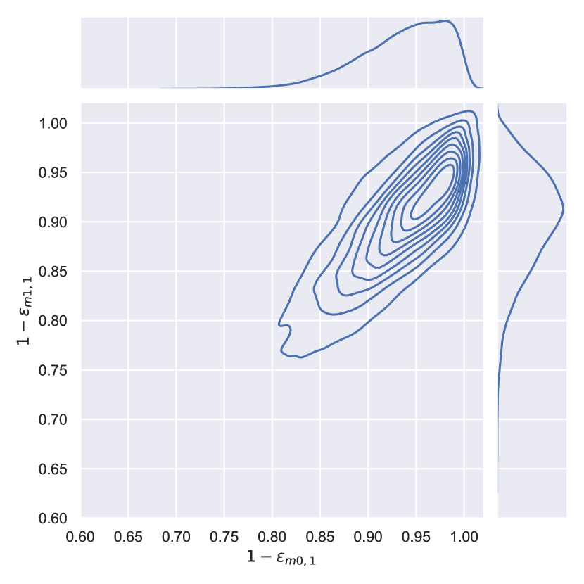
(a) Qubit 1

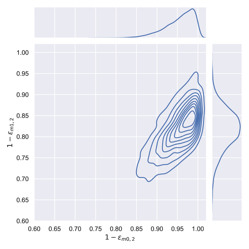
(b) Qubit 2

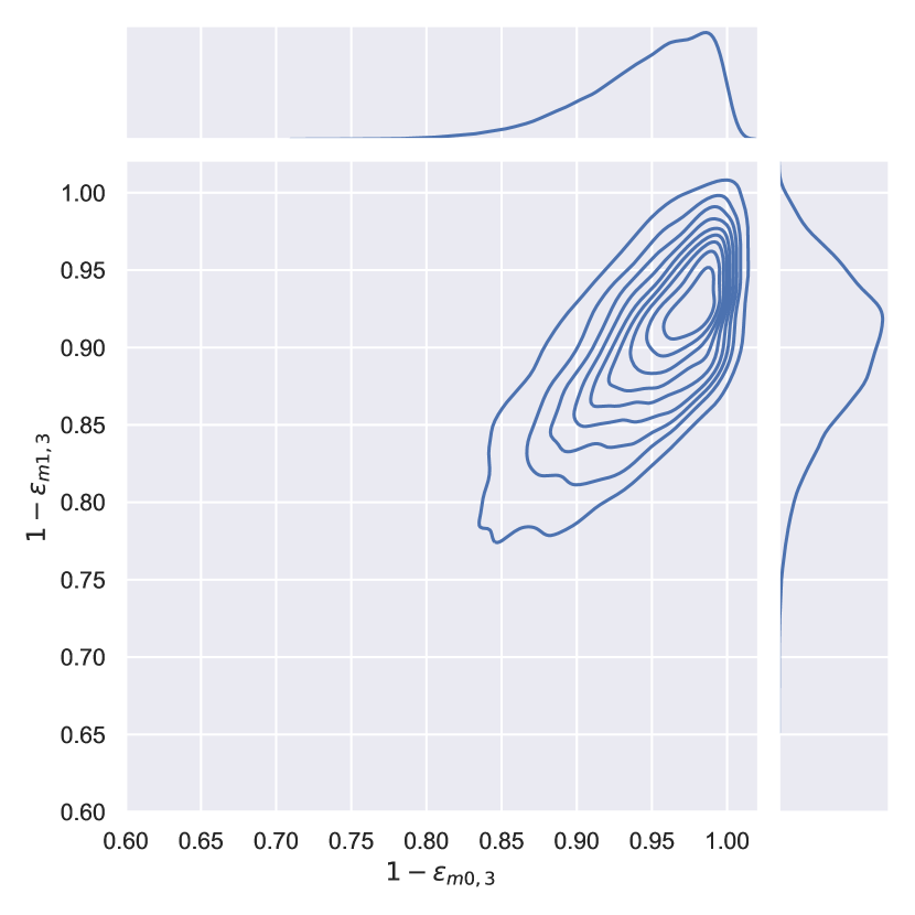
(c) Qubit 3

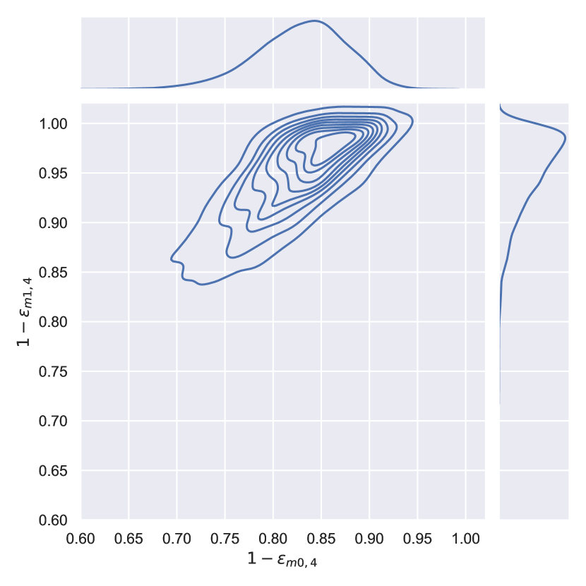
(d) Qubit 4

Figure 5: Joint and marginal posterior distributions of measurement error parameters in the testing circuit shown in Figure 4. Here, $(1-\epsilon_{m0,i},1-\epsilon_{m1,i})$ are shown for demonstration purpose.

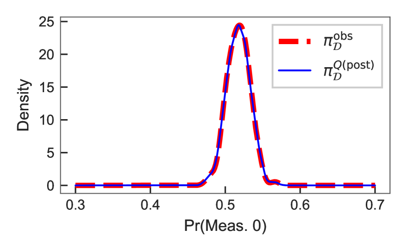
(a) Qubit 1

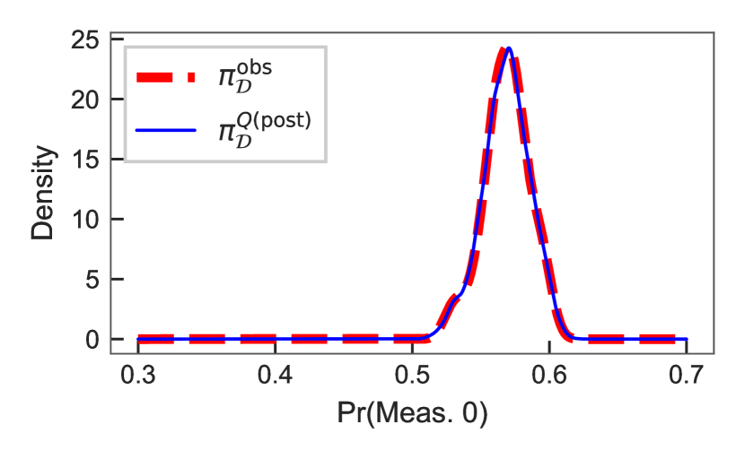
(b) Qubit 2

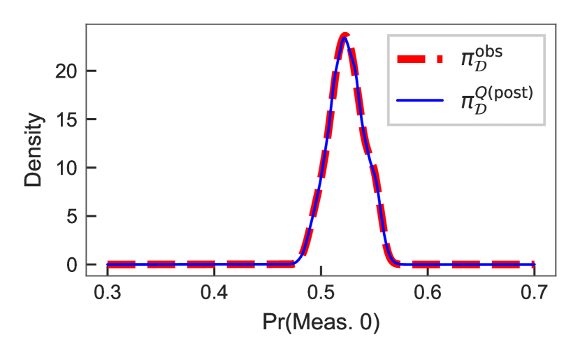
(c) Qubit 3

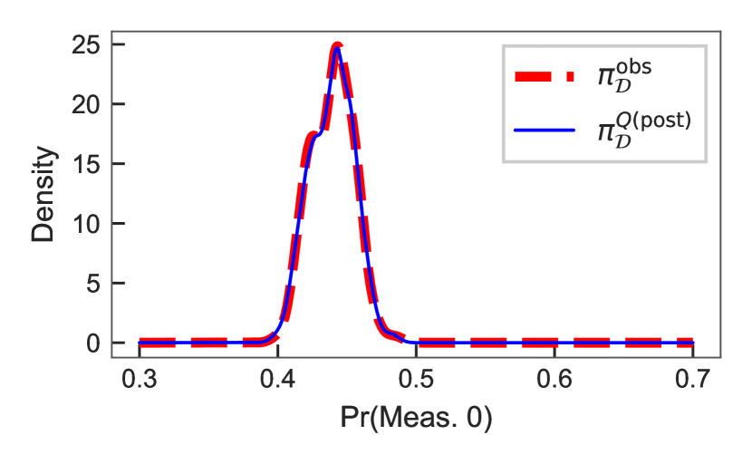
(d) Qubit 4

Figure 6: PDF of the QoI (i.e., the probability of measuring $\ket{0}$) obtained from data ($\pi_{\mathcal{D}}^{\text{obs}}$) and from evaluating $Q$ using inferred measurement error parameters ($\pi_{\mathcal{D}}^{Q(\text{post})}$).

For a more quantitative comparison, we list the posterior mean and the maximum a posteriori probability (MAP) in Table 1. We can see, in general, $\epsilon_{m1,i}$ is higher than $\epsilon_{m0,i}$, which is consistent with the description in [28]. Also, Tables 1 presents the Kullback–Leibler (KL) divergence between PDFs of the observed data $\pi_{\mathcal{D}}^{\text{obs}}$ and the posterior distribution of the QoI $\pi_{\mathcal{D}}^{Q(\text{post})}$ for each qubit in Figure 6, which illustrates the accuracy of our error model.

Table 1: Outcomes from the consistent Bayesian inference

	Qubit 1	Qubit 2	Qubit 3	Qubit 4
KL-div($\pi_{\mathcal{D}}^{Q(\text{posterior})},\pi_{\mathcal{D}}^{\text{obs}}$)	$0.001014$	$0.002243$	$0.000777$	$0.001610$
Post. Mean $(1-\epsilon_{m0,i},1-\epsilon_{m1,i})$	(0.9354,0.9009)	(0.9537,0.8184)	(0.9457,0.8976)	(0.8272,0.9492)
Post. MAP $(1-\epsilon_{m0,i},1-\epsilon_{m1,i})$	(0.9797,0.9128)	(0.9863,0.8243)	(0.9858,0.9180)	(0.8426,0.9846)

In this test, our prior distribution $N(\epsilon_{m0,i}^{0},0.1^{2})$ and $N(\epsilon_{m1,i}^{0},0.1^{2})$ are quite flat and not informative. This is because the vendor-provided $\epsilon_{m0,i}^{0}$ and $\epsilon_{m1,i}^{0}$ are not always good estimations. This can be verified by the error mitigation results. When we use relation Eq. (2) and Eq. (3) to construct measurement error filters using the vendor-provided $(\epsilon_{m0,i}^{0},\epsilon_{m1,i}^{0})$ and our posteriors, then apply those filters on the $128$ outputs of circuit in Figure 4 (i.e., $128$ observed probability of measuring $\ket{0}$), we obtain different results as shown in Figure 7. The theoretical probability of measuring $0$ for circuit in Figure 4 is $0.5$, but the provided parameters rarely gives this value, and its mean and peak of Gaussian KDE are not even close to $0.5$. On the other hand, the filters created by our posteriors can make sure the mean and peak of the denoised probability of measuring $\ket{0}$ are around the ideal value $0.5$. The results in Figure 4 indicate that when applying Eq. (3) to mitigate the measurement error, one has a larger chance to obtain a denoised QoI close to the ideal value $0.5$ by using the parameters inferred by our method. More importantly, the result by our method is unbiased as the mean value of the denoised QoI is $0.5$.

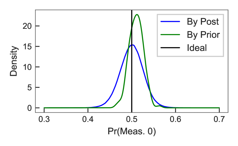
(a) Qubit 1

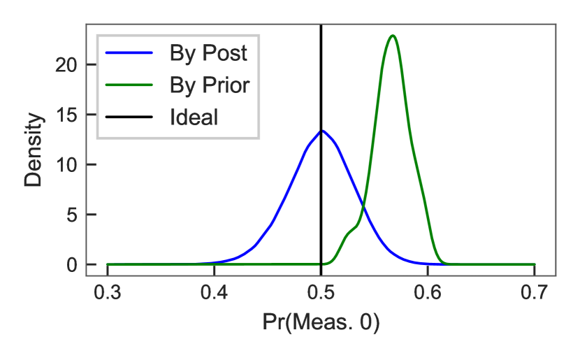
(b) Qubit 2

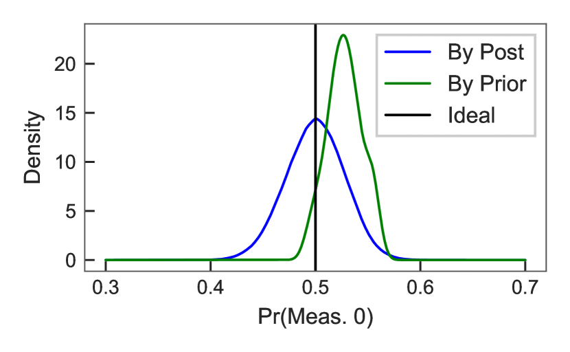
(c) Qubit 3

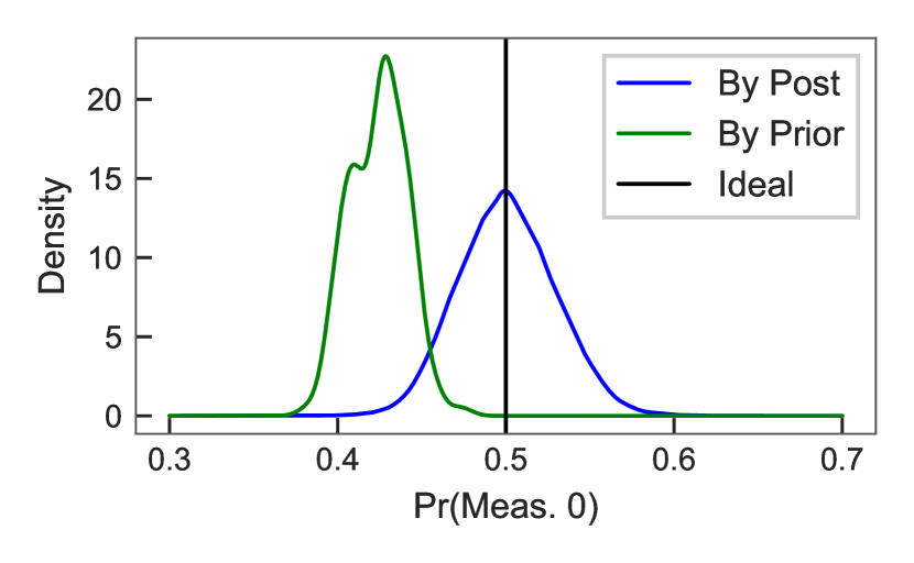
(d) Qubit 4

Figure 7: PDFs of the probability of measuring $\ket{0}$ denoised by vendor-provided parameters (priors) and by posteriors

This test indicates that we can use the circuit shown in Figure 4 to estimate measurement error in multiple qubits at the same time. It only requires to prepare initial state using ground states, and the total number of gates are linearly dependent on the number of qubits.

4.1.2 Application on State Tomography

After obtaining the error model parameters, we can further use this model mitigate the measurement errors in other circuits. We first apply error filters to the results of state tomography on circuits that make bell basis from $\ket{00}$ and $\ket{000}$. Qubit 0 and 1 are used for 2-qubit state and Qubit 0 to 2 are used for 3-qubit state in ibmqx2. The fidelity between density matrices from (corrected) state tomography result and theoretical quantum state is listed in Table 2. For the 2-qubit state tomography, filters constructed from posterior means by the consistent Bayesian and the standard Bayesian provides similar fidelity as that by the Qiskit filter. However, for 3-qubit tomography, filters from both Bayesian methods yield better fidelity, and their performance are similar. We note that the Qiskit filter assumes correlation in the measurements, which requires more model parameters, while our model does not. The fidelity in Table 2 indicates that Bayesian methods enable us to use fewer parameters to obtain better results.

Table 2: Fidelity of state tomography results filtered by various error filters

State	Fidelity
	Raw Data	By Qiskit Method	By Cons. Mean	By Stand. Mean
$\frac{1}{\sqrt{2}}(\ket{00}+\ket{11})$	0.9051	0.9800	0.9781	0.9783
$\frac{1}{\sqrt{2}}(\ket{01}+\ket{10})$	0.9157	0.9803	0.9806	0.9808
$\frac{1}{\sqrt{2}}(\ket{000}+\ket{111})$	0.7389	0.9227	0.9390	0.9391
$\frac{1}{\sqrt{2}}(\ket{010}+\ket{101})$	0.6719	0.8970	0.9203	0.9207
$\frac{1}{\sqrt{2}}(\ket{100}+\ket{011})$	0.7006	0.9121	0.9254	0.9207
$\frac{1}{\sqrt{2}}(\ket{110}+\ket{001})$	0.6974	0.8863	0.9443	0.9446

4.1.3 Application on Grover’s Search and QAOA

Next, we apply our filter on Grover’s search and QAOA circuits from [22]. We measure Qubit $1$ and $2$ in ibmqx2 for Grover’s search circuit. The exact solution of this Grover’s search example is $\ket{11}$ and the theoretical probability is $1$. Thus, in this case, we compare the probability of measuring $\ket{11}$ by running in the real device ibmqx2 and the denoised probabilities from error filters based on Qiskit method CompleteMeasFitter, QDT in [12], mean and MAP of posteriors from standard Bayesian, and mean and MAP of posteriors from the consistent Bayesian. All circuits for the Qiskit filter and QDT filters are executed for $8192$ shots, and each probability used in both filters is estimated from $8192$ measurement outcomes.

In addition, as we do not expect the quantum computer has a stable environment, in order to see the robustness of each method in comparison, after the data for creating error filters are collected, we run our Grover’s search circuit at several different time and then apply the same set of filters. All results are listed in Table 3.

Table 3: Probability of measuring $\ket{11}$ in Grover’s search example

Method/Source	Hour 0	Hour 2	Hour 4	Hour 8	Hour 12	Hour 16
Raw Data	0.6727	0.6930	0.6724	0.6740	0.6917	0.6841
Qiskit Method	0.7097	0.7335	0.7104	0.7120	0.7323	0.7241
QDT	0.7107	0.7332	0.7087	0.7108	0.7305	0.7224
Stand. Mean	0.9099	0.9324	0.9063	0.9088	0.9290	0.9192
Stand. MAP	0.8378	0.8635	0.8372	0.8392	0.8616	0.8522
Cons. Mean	0.9128	0.9351	0.9088	0.9114	0.9316	0.9219
Cons. MAP	0.8920	0.9158	0.8914	0.8936	0.9128	0.9034

As shown in Table 3, both Bayesian methods yield best performance among all the methods while the filters constructed from posterior mean are better than the filters constructed from posterior MAP. In all six time slots, the mean and MAP from the consistent Bayesian provide sightly better denoising effect than those from the standard Bayesian.

The QAOA example includes two rounds and parameters for QAOA circuits are set as $(\gamma_{1},\beta_{1})=(0.2\pi,0.15\pi)$ and $(\gamma_{2},\beta_{2})=(0.4\pi,0.05\pi)$ [22]. The graph of the QAOA example in [22] is shown in Figure 8, which has maximum objective value $3$ in Max-Cut problem and 6 bit-string optimal solution $\ket{0010}$, $\ket{0101}$, $\ket{0110}$, $\ket{1001}$, $\ket{1010}$, $\ket{1101}$ (ibmqx2 uses little-endien convention, so the rightmost bit is Node 1 and the leftmost bit is Node 4). Because the graph in Figure 8 is a subgraph of the coupling map of ibmqx2, we map the nodes to qubits exactly.

Figure 8: The graph of QAOA example in [22]

The average size of a cut and the probability of measuring an optimal solution are two quantities to compare in this experiment. Moreover, the results from simulator is also provided as a indicator for the situation without noise. The remaining procedures are the same as those in Grover’s search experiment. The data is reported in Table 4 and 5. Here, “QDT” error filter from [12] is built under the assumption that measurement operations are independent between each qubit due to the large amount of testing circuits that correlation assumption requires ($6^{4}$ circuits if assume qubits are correlated in measurement).

Table 4: Average size of a sampled cut in QAOA example

Method/Source	Hour 0	Hour 2	Hour 4	Hour 8	Hour 12	Hour 16
Simulator	2.8637	2.8642	2.8651	2.8652	2.8642	2.8626
Raw Data	2.3005	2.3579	2.3197	2.2823	2.3063	2.2871
Qiskit Method	2.3783	2.4623	2.4247	2.3786	2.4063	2.3926
QDT	2.3812	2.4453	2.4016	2.3589	2.3851	2.3612
Stand. Mean	2.4878	2.5483	2.5059	2.4551	2.4860	2.4581
Stand. MAP	2.4080	2.4708	2.4222	2.3800	2.4059	2.3829
Cons. Mean	2.4911	2.5518	2.5089	2.4578	2.4891	2.4612
Cons. MAP	2.4407	2.4996	2.4554	2.4109	2.4382	2.4133

Table 5: Probability of measuring an optimal solution in QAOA example

Method/Source	Hour 0	Hour 2	Hour 4	Hour 8	Hour 12	Hour 16
Simulator	0.8930	0.8937	0.8941	0.8943	0.8940	0.8940
Raw Data	0.5784	0.6038	0.5895	0.5725	0.5748	0.5740
Qiskit Method	0.5968	0.6456	0.6316	0.6074	0.6140	0.6155
QDT	0.6400	0.6698	0.6525	0.6312	0.6331	0.6325
Stand. Mean	0.6952	0.7239	0.7033	0.6766	0.6787	0.6797
Stand. MAP	0.6444	0.6695	0.6508	0.6305	0.6309	0.6317
Cons. Mean	0.6975	0.7265	0.7058	0.6790	0.6810	0.6822
Cons. MAP	0.6610	0.6860	0.6672	0.6431	0.6439	0.6452

The conclusion from Table 4 and 5 is basically the same as that from Table 3. Namely, Bayesian methods, especially filters from posterior mean, outperform other methods, and parameters inferred by the consistent Bayesian works slightly better than those by the standard Bayesian in all six time slots. From both Grover’s search and QAOA examples, we can see the accuracy of both Bayesian approaches are better than the existing methods.

4.1.4 Application on Random Clifford Circuits

Finally, we test the measurement-error filtering for random 2-Qubit Clifford circuits with 1, 2, 3, and 4 2-Qubit Clifford operators (i.e., length 1, 2, 3, 4). For each length, $16$ random circuits are generated to draw a boxplot and each circuit is run for $8192$ shots. The results are shown in Figure 9. While the theoretical output of 2-Qubit Clifford circuit is $\ket{00}$ with probability 1, Figure 9 demonstrate that the filter constructed from posterior mean estimated by standard Bayesian provides best performance. The consistent Bayesian results in almost the same results as the standard Bayesian method.

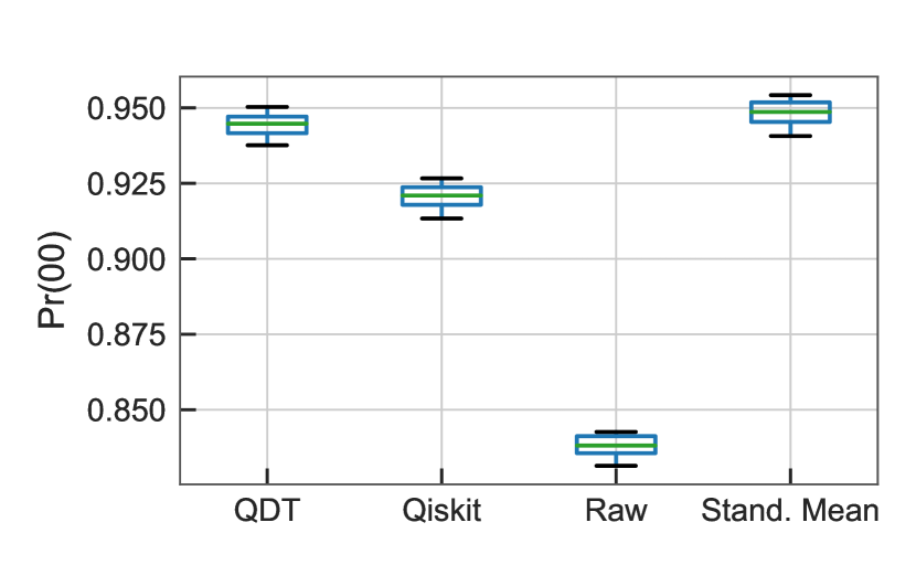
(a) Length 1

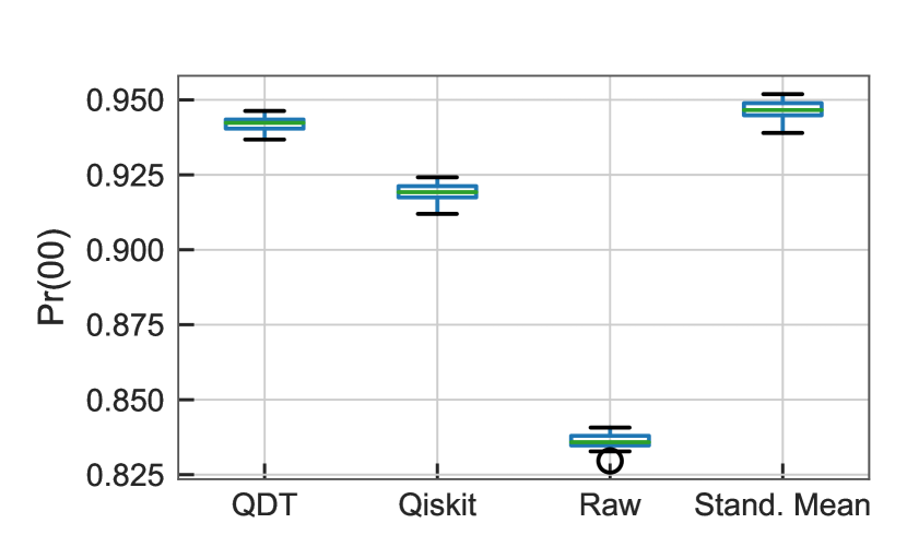
(b) Length 2

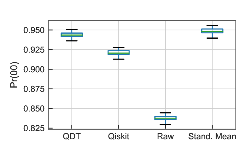
(c) Length 3

(d) Length 4

Figure 9: Measurement-error filtering for random 2-Qubit Clifford circuits. “Length” represents the number of Clifford operators in the circuit. “Probability” means the probability of measuring $\ket{00}$.

4.2 Gate and Measurement Error Filtering Experiment

We consider the circuit with $200$ NOT gates as shown in Figure 10. We still use machine ibmqx2 and run the experiment twice separately on Qubit 1 and Qubit 2. In each trial, the circuit is executed $1024\times 128$ times where readouts from every $1024$ runs are used to estimate the QoI, i.e., the probability of measuring $\ket{0}$. Namely, we collect $128$ samples of the QoI.

Figure 10: Experiment circuit for gate and measurement error mitigation.

Because the aforementioned Qiskit method CompleteMeasFitter and QDT are for measurement errors, in this section, we only compare the results from standard Bayesian and the consistent Bayesian with the same priors and dataset. The priors are truncated normal $N(\epsilon_{m0,i}^{0},0.1^{2})$, $N(\epsilon_{m1,i}^{0},0.1^{2})$, and $N(\epsilon_{g,i}^{0},0.005^{2})$ with range $(0,1)$. Again, $\epsilon_{m0,i}^{0},\epsilon_{m1,i}^{0},\epsilon_{g,i}^{0}$ are vendor-provided values from IBM’s daily calibration and standard deviations are chosen to make prior relatively flat due to the lack of knowledge on these parameters.

4.2.1 Inference for Noise Parameters

Figure 11 shows the distribution of $\epsilon_{g}$ in Qubit 1 and 2. Both distributions are right-skewed. Table 6 provides the numerical values for mean and MAP. In Table 6, we can see both methods give similar measurement error parameter $\epsilon_{m0,i}$ and $\epsilon_{m1,i}$ on Qubit 1 and 2, but the gate error rate $\epsilon_{g}$ are not always similar. More importantly, as shown in Figure 12, posteriors of the QoI from the consistent Bayesianp, i.e., $\pi_{\mathcal{D}}^{Q(\text{post})}$ matches the distribution of data, i.e., $\pi_{\mathcal{D}}^{\text{obs}}$ quite well. On the other hand, the posterior distribution of the QoI generated by posteriors distributions of model parameters from the standard Bayesian can match the empirial mean of the data only while the shape of the PDF is quite different.

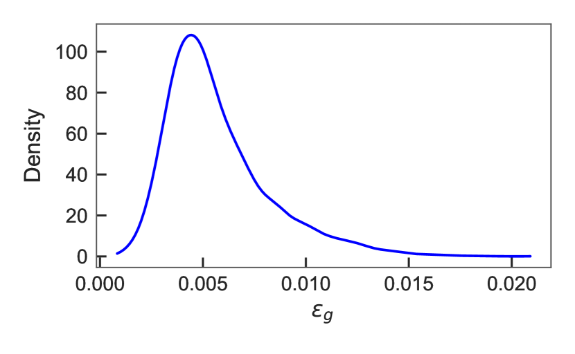
(a) Qubit 1

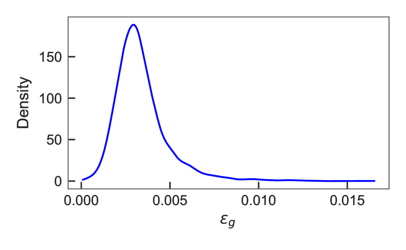
(b) Qubit 2

Figure 11: Gaussian KDE of $\epsilon_{g}$

Table 6: Measurement error parameters of the consistent and standard Bayesian inference.

	Qubit 1	Qubit 2
Consistent Post. Mean $(1-\epsilon_{m0,i},1-\epsilon_{m1,i},\epsilon_{g})$	(0.9255, 0.8922, 0.004934)	(0.9229, 0.8856, 0.003804)
Consistent Post. MAP $(1-\epsilon_{m0,i},1-\epsilon_{m1,i},\epsilon_{g})$	(0.9756, 0.8837, 0.004827)	(0.9770, 0.9485, 0.003291)
Standard Post. Mean $(1-\epsilon_{m0,i},1-\epsilon_{m1,i},\epsilon_{g})$	(0.9221, 0.8939, 0.004683)	(0.9214, 0.8871, 0.002982)
Standard Post. MAP $(1-\epsilon_{m0,i},1-\epsilon_{m1,i},\epsilon_{g})$	(0.9758, 0.8835, 0.006550)	(0.9836, 0.9354, 0.003453)

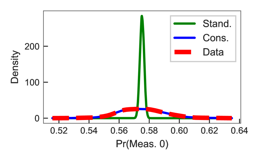
(a) Qubit 1

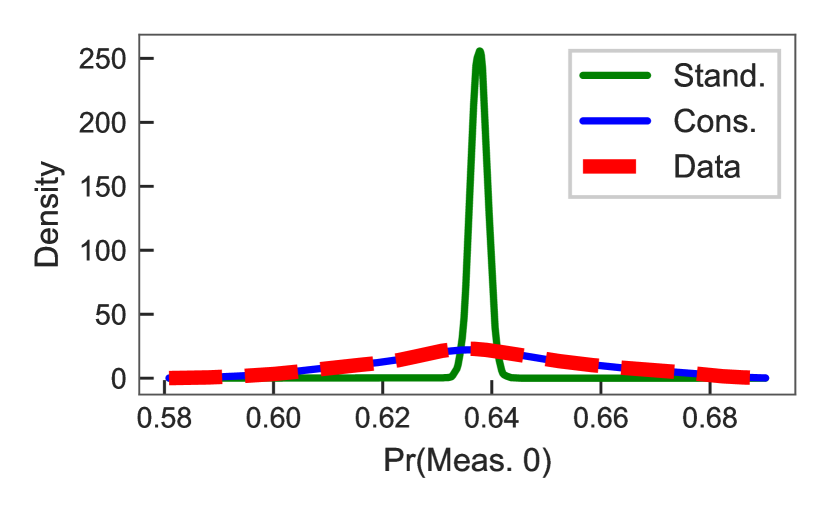
(b) Qubit 2

Figure 12: Posterior distribution of the QoI, i.e., $\pi_{\mathcal{D}}^{Q(\text{post})}$, generated by the posterior distribution of model parameters from both Bayesian methods

4.2.2 Error Filtering

Using the posterior means from Table 6, we construct gate and measurement error filters and apply them on the 128 samples of the QoI. (i.e., probabilities of measuring 0) on Qubit 1 and Qubit 2. The results are displayed in Figure 13. It shows that both Bayesian approaches we use can recover the exact value $1$ with high probability. More importantly, the consistent Bayesian outperforms the standard one as it recovers the exact value $1$ with larger chance. especially in the test on Qubit 2.

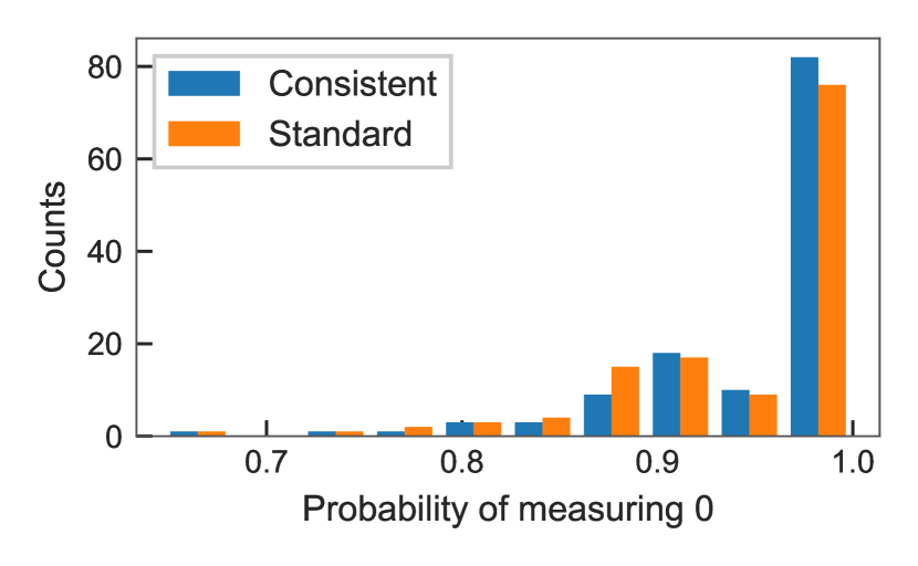
(a) Qubit 1

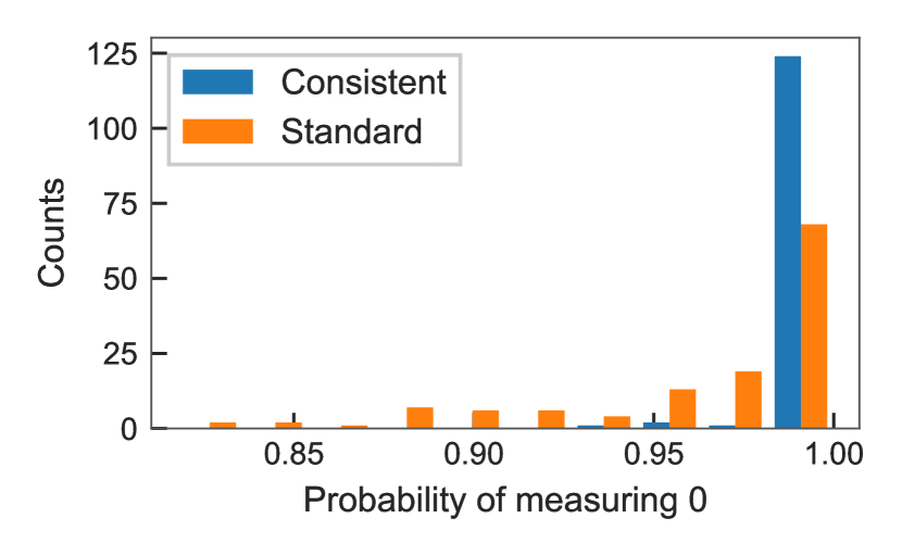
(b) Qubit 2

Figure 13: Denoised (both gate and measurement) probability of measuring 0. Parameters used are posterior mean from Table 6.

The data for error filters in Section 4.1 and experiment in Section 4.2 were collected within one hour, so it is reasonable to use posteriors in Section 4.2 to denoise the Grover’s search data in Section 4.1. However, comparing the values of measurement error parameters in Table 1 and in Table 6, we can see there are some noticeable differences. Table 7 provides the results of using parameters in Section 4.2 to filter out errors in data used in Section 4.1. We can see they are better than Qiskit method and QDT, but worse than values from either Bayesian methods shown in Tabel 3.

Table 7: Probability of measuring $\ket{11}$ in Grover’s search Example denoised by parameters in Section 4.2

Method	Hour 0	Hour 2	Hour 4	Hour 8	Hour 12	Hour 16
Stand. Mean	0.8398	0.8680	0.8392	0.8414	0.8656	0.8561
Stand. MAP	0.8116	0.8367	0.8110	0.8131	0.8348	0.8257
Cons. Mean	0.8434	0.8716	0.8428	0.8450	0.8691	0.8595
Cons. MAP	0.7992	0.8240	0.7986	0.8005	0.8221	0.8131

One possible explanation is, with $200$ gates, our model is much more sensitive to the gate error than the measurement error. A comparison of the sensitivity is shown in Figure 14, where the results are obtained by using the error models Eqs. (2) and (6). In Figure 14 (a) and (b), we can see that when $\epsilon_{g}$ is fixed, the QoI changes linearly and slowly as $\epsilon_{m0,i}$ or $\epsilon_{m1,i}$ varies. However, as shown in Figure 14 (c) when $\epsilon_{m0,i}$ and $\epsilon_{m1,i}$ are fixed, the QoI changes rapidly as $\epsilon_{g}$ increases. the estimation of measurement error in Section 4.1 uses circuits that have 0.5 chance to measure either $\ket{0}$ or $\ket{1}$ without noise and this distribution does not change when a Hadamard gate suffers from bit-flip or phase-flip error, so it yields a better performance.

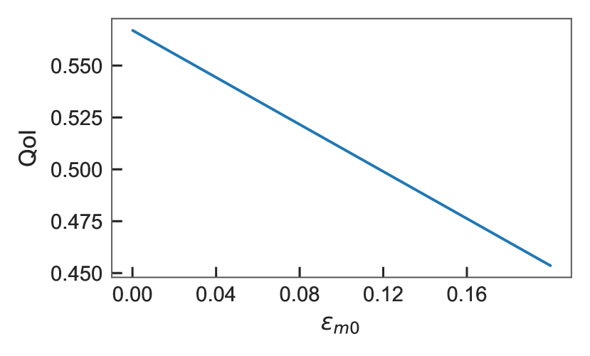
(a) $\epsilon_{m1}=0,\epsilon_{g}=0.005$

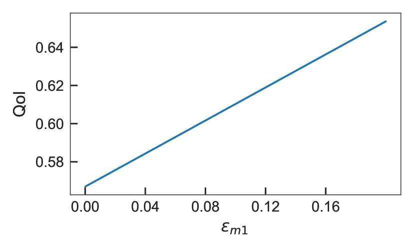
(b) $\epsilon_{m1}=0,\epsilon_{g}=0.005$

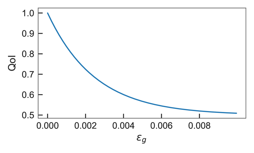
(c) $\epsilon_{m1}=0,\epsilon_{m0}=0$

Figure 14: Sensitivity analysis of forward model $Q$ with 200 NOT gate.

5 Discussion and Future Works

In this work, we extend a bit-flip error model from a single gate case to multiple gate case, and provide theoretical analysis to prove the existence of the error mitigation solution for both cases. In some noise models, such as depolarizing error model, the rate of bit-flip error is associated with the rates of other types of errors [29, p. 379]. Thus, the inference of bit-flip error rates could provide a connection to a more general noise model. We propose to use Bayesian approaches to infer parameters in the error models to characterize the propagation of the device noise in QC algorithms more effectively. The experiments in Section 4 demonstrate that our methodology outperforms two existing methods on the same error models over a wide range of time, while the number of testing circuits is linear or constant to the number of qubits. The consistent Bayesian approach is, in general, better than the standard Bayesian. These results indicate that our error models can characterize the device noise quite well, and they help to understand the propagation of such noise in QC algorithms.

There are still several limitations in our methodology. One issue that affects the scalability of our method is the exponentially large matrix in the denoising step. The dimension of matrices can be reduced if we can identify the qubits that are independent during the measurement step of an algorithm and filter their measurement outcome separately. A recent work in [30] also indicates a scheme to reduce the dimension of the transition matrix by limiting the range of bases that are put into consideration. Also, a parallel algorithm proposed in [31] can exploit the tensor-product structure of the linear system in the error filtering step to speedup the calculation. On the other hand, because the method of estimating the distribution of model parameters is not limited by the two models we discussed in the paper, a consideration for pairwise-correlated measurement error model discussed in [13] probably be helpful for inferring correlated measurement error rates. A potential extension to the applicable gates is to modify the model to accommodate multi-qubit bit-flip error instead of individual-qubit error. This is because more gates commute with $X^{\otimes n}$ than with elements in $\{X,I\}^{\otimes n}$ for $n\geq 2$. For example, $X\otimes X$ commute with matrix $A\otimes B$ and $e^{-i\delta A\otimes B}$ for $(A,B)\in\{Y,Z\}^{\otimes 2}\cup\{I,X\}^{\otimes 2}$ and arbitrary $\delta$, where the form $e^{-i\delta A\otimes B}$ is generally utilized in quantum simulation [32].

References

- [1] John Preskill. Quantum computing in the NISQ era and beyond. Quantum, 2:79, August 2018.
- [2] Robert Raussendorf and Jim Harrington. Fault-tolerant quantum computation with high threshold in two dimensions. Physical Review Letters, 98(19), May 2007.
- [3] Aleksander Marek Kubica. The ABCs of the Color Code: A Study of Topological Quantum Codes as Toy Models for Fault-Tolerant Quantum Computation and Quantum Phases Of Matter. PhD thesis, California Institute of Technology, 2018.
- [4] Dorit Aharonov and Michael Ben-Or. Fault-tolerant quantum computation with constant error rate. SIAM Journal on Computing, 38(4):1207–1282, January 2008.
- [5] C. Flühmann, T. L. Nguyen, M. Marinelli, V. Negnevitsky, K. Mehta, and J. P. Home. Encoding a qubit in a trapped-ion mechanical oscillator. Nature, 566(7745):513–517, February 2019.
- [6] Arne L. Grimsmo, Joshua Combes, and Ben Q. Baragiola. Quantum computing with rotation-symmetric bosonic codes. Physical Review X, 10(1), March 2020.
- [7] Atharv Joshi, Kyungjoo Noh, and Yvonne Y Gao. Quantum information processing with bosonic qubits in circuit qed. Quantum Science and Technology, 6(3):033001, 2021.
- [8] Joel J. Wallman and Joseph Emerson. Noise tailoring for scalable quantum computation via randomized compiling. Physical Review A, 94(5), November 2016.
- [9] Kristan Temme, Sergey Bravyi, and Jay M. Gambetta. Error mitigation for short-depth quantum circuits. Physical Review Letters, 119(18), November 2017.
- [10] Suguru Endo, Simon C. Benjamin, and Ying Li. Practical quantum error mitigation for near-future applications. Physical Review X, 8(3), July 2018.
- [11] Abhinav Kandala, Kristan Temme, Antonio D Córcoles, Antonio Mezzacapo, Jerry M Chow, and Jay M Gambetta. Error mitigation extends the computational reach of a noisy quantum processor. Nature, 567(7749):491–495, 2019.
- [12] Filip B. Maciejewski, Zoltán Zimborás, and Michał Oszmaniec. Mitigation of readout noise in near-term quantum devices by classical post-processing based on detector tomography. Quantum, 4:257, April 2020.
- [13] Sergey Bravyi, Sarah Sheldon, Abhinav Kandala, David C. Mckay, and Jay M. Gambetta. Mitigating measurement errors in multiqubit experiments. Phys. Rev. A, 103:042605, Apr 2021.
- [14] Google AI Quantum and Collaborators, Frank Arute, Kunal Arya, Ryan Babbush, Dave Bacon, Joseph C. Bardin, Rami Barends, Sergio Boixo, Michael Broughton, Bob B. Buckley, David A. Buell, Brian Burkett, Nicholas Bushnell, Yu Chen, Zijun Chen, Benjamin Chiaro, Roberto Collins, William Courtney, Sean Demura, Andrew Dunsworth, Edward Farhi, Austin Fowler, Brooks Foxen, Craig Gidney, Marissa Giustina, Rob Graff, Steve Habegger, Matthew P. Harrigan, Alan Ho, Sabrina Hong, Trent Huang, William J. Huggins, Lev Ioffe, Sergei V. Isakov, Evan Jeffrey, Zhang Jiang, Cody Jones, Dvir Kafri, Kostyantyn Kechedzhi, Julian Kelly, Seon Kim, Paul V. Klimov, Alexander Korotkov, Fedor Kostritsa, David Landhuis, Pavel Laptev, Mike Lindmark, Erik Lucero, Orion Martin, John M. Martinis, Jarrod R. McClean, Matt McEwen, Anthony Megrant, Xiao Mi, Masoud Mohseni, Wojciech Mruczkiewicz, Josh Mutus, Ofer Naaman, Matthew Neeley, Charles Neill, Hartmut Neven, Murphy Yuezhen Niu, Thomas E. O’Brien, Eric Ostby, Andre Petukhov, Harald Putterman, Chris Quintana, Pedram Roushan, Nicholas C. Rubin, Daniel Sank, Kevin J. Satzinger, Vadim Smelyanskiy, Doug Strain, Kevin J. Sung, Marco Szalay, Tyler Y. Takeshita, Amit Vainsencher, Theodore White, Nathan Wiebe, Z. Jamie Yao, Ping Yeh, and Adam Zalcman. Hartree-fock on a superconducting qubit quantum computer. Science, 369(6507):1084–1089, 2020.
- [15] Yanzhu Chen, Maziar Farahzad, Shinjae Yoo, and Tzu-Chieh Wei. Detector tomography on IBM quantum computers and mitigation of an imperfect measurement. Physical Review A, 100(5), November 2019.
- [16] Michael R Geller. Rigorous measurement error correction. Quantum Science and Technology, 5(3):03LT01, June 2020.
- [17] Lena Funcke, Tobias Hartung, Karl Jansen, Stefan Kühn, Paolo Stornati, and Xiaoyang Wang. Measurement error mitigation in quantum computers through classical bit-flip correction. Physical Review A, 105(6):062404, 2022.
- [18] Yasuhiro Takahashi, Yuki Takeuchi, and Seiichiro Tani. Classically Simulating Quantum Circuits with Local Depolarizing Noise. In Javier Esparza and Daniel Kráľ, editors, 45th International Symposium on Mathematical Foundations of Computer Science (MFCS 2020), volume 170 of Leibniz International Proceedings in Informatics (LIPIcs), pages 83:1–83:13, Dagstuhl, Germany, 2020. Schloss Dagstuhl–Leibniz-Zentrum für Informatik.
- [19] T. Butler, J. Jakeman, and T. Wildey. Combining push-forward measures and bayes' rule to construct consistent solutions to stochastic inverse problems. SIAM Journal on Scientific Computing, 40(2):A984–A1011, January 2018.
- [20] Sarah Sheldon, Easwar Magesan, Jerry M. Chow, and Jay M. Gambetta. Procedure for systematically tuning up cross-talk in the cross-resonance gate. Physical Review A, 93(6), June 2016.
- [21] Frank Arute, Kunal Arya, Ryan Babbush, Dave Bacon, Joseph C. Bardin, Rami Barends, Rupak Biswas, Sergio Boixo, Fernando G. S. L. Brandao, David A. Buell, Brian Burkett, Yu Chen, Zijun Chen, Ben Chiaro, Roberto Collins, William Courtney, Andrew Dunsworth, Edward Farhi, Brooks Foxen, Austin Fowler, Craig Gidney, Marissa Giustina, Rob Graff, Keith Guerin, Steve Habegger, Matthew P. Harrigan, Michael J. Hartmann, Alan Ho, Markus Hoffmann, Trent Huang, Travis S. Humble, Sergei V. Isakov, Evan Jeffrey, Zhang Jiang, Dvir Kafri, Kostyantyn Kechedzhi, Julian Kelly, Paul V. Klimov, Sergey Knysh, Alexander Korotkov, Fedor Kostritsa, David Landhuis, Mike Lindmark, Erik Lucero, Dmitry Lyakh, Salvatore Mandrà, Jarrod R. McClean, Matthew McEwen, Anthony Megrant, Xiao Mi, Kristel Michielsen, Masoud Mohseni, Josh Mutus, Ofer Naaman, Matthew Neeley, Charles Neill, Murphy Yuezhen Niu, Eric Ostby, Andre Petukhov, John C. Platt, Chris Quintana, Eleanor G. Rieffel, Pedram Roushan, Nicholas C. Rubin, Daniel Sank, Kevin J. Satzinger, Vadim Smelyanskiy, Kevin J. Sung, Matthew D. Trevithick, Amit Vainsencher, Benjamin Villalonga, Theodore White, Z. Jamie Yao, Ping Yeh, Adam Zalcman, Hartmut Neven, and John M. Martinis. Quantum supremacy using a programmable superconducting processor. Nature, 574(7779):505–510, October 2019.
- [22] J. Abhijith, Adetokunbo Adedoyin, John Ambrosiano, Petr Anisimov, Andreas Bärtschi, William Casper, Gopinath Chennupati, Carleton Coffrin, Hristo Djidjev, David Gunter, Satish Karra, Nathan Lemons, Shizeng Lin, Alexander Malyzhenkov, David Mascarenas, Susan Mniszewski, Balu Nadiga, Daniel O’Malley, Diane Oyen, Scott Pakin, Lakshman Prasad, Randy Roberts, Phillip Romero, Nandakishore Santhi, Nikolai Sinitsyn, Pieter J. Swart, James G. Wendelberger, Boram Yoon, Richard Zamora, Wei Zhu, Stephan Eidenbenz, Patrick J. Coles, Marc Vuffray, and Andrey Y. Lokhov. Quantum Algorithm Implementations for Beginners. arXiv e-prints, page arXiv:1804.03719, April 2018.
- [23] Muqing Zheng. Qcol-lu/bayesian-error-characterization-and-mitigation, August 2022.
- [24] Ryan ODonnell. Analysis of boolean functions. Cambridge University Press, 2014.
- [25] Stan Development Team. RStan: the R interface to Stan, 2020. R package version 2.21.1.
- [26] R Core Team. R: A Language and Environment for Statistical Computing. R Foundation for Statistical Computing, Vienna, Austria, 2019. R version 3.6.2.
- [27] Gadi Aleksandrowicz, Thomas Alexander, Panagiotis Barkoutsos, Luciano Bello, Yael Ben-Haim, David Bucher, Francisco Jose Cabrera-Hernández, Jorge Carballo-Franquis, Adrian Chen, Chun-Fu Chen, Jerry M. Chow, Antonio D. Córcoles-Gonzales, Abigail J. Cross, Andrew Cross, Juan Cruz-Benito, Chris Culver, Salvador De La Puente González, Enrique De La Torre, Delton Ding, Eugene Dumitrescu, Ivan Duran, Pieter Eendebak, Mark Everitt, Ismael Faro Sertage, Albert Frisch, Andreas Fuhrer, Jay Gambetta, Borja Godoy Gago, Juan Gomez-Mosquera, Donny Greenberg, Ikko Hamamura, Vojtech Havlicek, Joe Hellmers, Łukasz Herok, Hiroshi Horii, Shaohan Hu, Takashi Imamichi, Toshinari Itoko, Ali Javadi-Abhari, Naoki Kanazawa, Anton Karazeev, Kevin Krsulich, Peng Liu, Yang Luh, Yunho Maeng, Manoel Marques, Francisco Jose Martín-Fernández, Douglas T. McClure, David McKay, Srujan Meesala, Antonio Mezzacapo, Nikolaj Moll, Diego Moreda Rodríguez, Giacomo Nannicini, Paul Nation, Pauline Ollitrault, Lee James O’Riordan, Hanhee Paik, Jesús Pérez, Anna Phan, Marco Pistoia, Viktor Prutyanov, Max Reuter, Julia Rice, Abdón Rodríguez Davila, Raymond Harry Putra Rudy, Mingi Ryu, Ninad Sathaye, Chris Schnabel, Eddie Schoute, Kanav Setia, Yunong Shi, Adenilton Silva, Yukio Siraichi, Seyon Sivarajah, John A. Smolin, Mathias Soeken, Hitomi Takahashi, Ivano Tavernelli, Charles Taylor, Pete Taylour, Kenso Trabing, Matthew Treinish, Wes Turner, Desiree Vogt-Lee, Christophe Vuillot, Jonathan A. Wildstrom, Jessica Wilson, Erick Winston, Christopher Wood, Stephen Wood, Stefan Wörner, Ismail Yunus Akhalwaya, and Christa Zoufal. Qiskit: An Open-source Framework for Quantum Computing, January 2019. Version 0.14.2.
- [28] Rebecca Hicks, Christian W. Bauer, and Benjamin Nachman. Readout rebalancing for near-term quantum computers. Physical Review A, 103(2), February 2021.
- [29] Michael A. Nielsen and Isaac L. Chuang. Quantum computation and quantum information. Cambridge University Press, 2010.
- [30] Paul D. Nation, Hwajung Kang, Neereja Sundaresan, and Jay M. Gambetta. Scalable mitigation of measurement errors on quantum computers. arXiv e-prints, page arXiv:2108.12518, August 2021.
- [31] Paul E. Buis and Wayne R. Dyksen. Efficient vector and parallel manipulation of tensor products. ACM Transactions on Mathematical Software, 22(1):18–23, March 1996.
- [32] Francesco Tacchino, Alessandro Chiesa, Stefano Carretta, and Dario Gerace. Quantum computers as universal quantum simulators: State-of-the-art and perspectives. Advanced Quantum Technologies, 3(3):1900052, December 2019.