On thermal radiation of de Sitter space in the semiclassical Jackiw-Teitelboim model

Abstract

In general, the Gibbons-Hawking temperature based on the Euclidean functional approach shows that de Sitter space in the Bunch-Davies vacuum is globally thermal. In the exactly soluble semiclassical Jackiw-Teitelboim model, we investigate thermal property of de Sitter space by taking into account the quantum back reaction of the geometry. The proper temperature of de Sitter space in the Bunch-Davies vacuum is found to vanish. In case of a certain quantum state breaking the de Sitter symmetry, de Sitter space can be made thermally exited; however, in this case the dilaton singularity cannot be avoided. Consequently, in the Jackiw-Teitelboim model the proper temperature of de Sitter space in the Bunch-Davies vacuum turns out to be zero and the Bunch-Davies vacuum is found to be the only physical vacuum without any naked singularities.

I introduction

Since a spacetime during inflation can be approximated as de Sitter space of a vacuum solution of the Einstein equation with a positive cosmological constant, de Sitter space has been extensively studied in cosmology. For example, the slow-roll inflation Linde:1981mu ; Albrecht:1982wi ; Linde:1983gd ; Ade:2015lrj is typically assumed to begin with the quantum state describing perturbations in the Bunch-Davies vacuum as a de Sitter-invariant vacuum of de Sitter space Nelson:2012ax . In fact, Hawking radiation in de Sitter phase of an inflationary universe is the source of primordial matter fluctuations and classical energy-density perturbations that may explain the origin of galaxies (for a review, see Ref. Brandenberger:1984cz ).

Using the Euclidean functional approach, Gibbons and Hawking Gibbons:1977mu showed that for freely falling observers the propagator for a scalar field was turned out to be a periodic function of a time with period $i\beta$. This is the characteristic of thermal Green’s functions with a temperature $T=\beta^{-1}$. In thermal equilibrium the temperature is identified with the surface gravity at the cosmological horizon as

$$T_{\rm GH}=\frac{H}{2\pi},$$ (1)

where $H$ is the Hubble constant. It should be emphasized that the Gibbons and Hawking’s formulation is based on the belief that a well-defined meaning for the Green’s function can be given by analytically continuing back to the original Lorentzian spacetime from the Euclidean metric.

On the other hand, in the stress tensor approach, it has been known that the temperature in thermal equilibrium can be derived from the Stefan-Boltzmann law Tolman:1930zza ; Tolman:1930ona . However, in two-dimensional de Sitter space, this procedure fails since one immediately confronts a negative energy density as

$$\epsilon=-\langle T^{0}_{0}\rangle_{\rm BD}=-\frac{H^{2}}{24\pi}=\gamma_{(2)}T^{2}_{\rm GH},$$ (2)

where $\gamma_{(2)}=\pi/6$ for a single massless scalar field. This fact is not new since the negative sign of the energy density was already pointed out in Ref. Markkanen:2017abw . The usual Stefan-Boltzmann law renders the Gibbons-Hawking temperature to be imaginary, so it does not meet the stress tensor approach. Now, in the stress tensor approach, it raises a question about how to define the proper temperature of two-dimensional de Sitter space in thermal equilibrium. Thus, we are going to study this issue both on the de Sitter background and from the dynamical point of view, in the semiclassically quantized Jackiw-Teitelboim model with a positive cosmological constant Teitelboim:1983ux ; Jackiw:1984je , respectively.

In thermal equilibrium, it is worth noting that Tolman derived the Stefan-Boltzmann on the curved spacetime by assuming that the stress tensor is traceless Tolman:1930zza ; Tolman:1930ona ; however, this fact was sometimes ignored. In this regard, the Stefan-Boltzmann law for the non-vanishing trace of the stress tensor should be modified in such a way that the trace anomaly of the stress tensor must be appropriately taken into account in the thermodynamic first law Gim:2015era . In fact, for a non-vanishing trace of the stress tensor, the modified Stefan-Boltzmann law was successfully applied to a cosmological model for reheating of our universe Gim:2016uvv and black hole models related to quantum atmosphere Unruh:1977ga ; Giddings:2015uzr ; Eune:2015xvx ; Kim:2016iyf ; Eune:2017iab ; Eune:2019aat . Since the trace of stress tensor on the de Sitter space is also non-vanishing Davies:1977ze ; 10.2307/79520 ; Christensen:1977jc ; Deser:1976yx , we shall apply this modified Stefan-Boltzmann law to de Sitter space in the stress tensor approach, and will resolve the imaginary temperature problem in Eq. (2).

The organization of this paper is as follows. In Sec. II, we will calculate the proper temperature of de Sitter space by using the renormalized stress tensor from the one-loop Polyakov effective action of free scalar fields and obtain the vanishing proper temperature in the Bunch-Davies vacuum by using the modified Stefan-Boltzmann law. In Sec. III, we will revisit thermal property of de Sitter space by embedding de Sitter space in the semiclassically quantized Jackiw-Teitelboim model, and obtain the same result as that of Sec. III: the proper temperature in the Bunch-Davies vacuum vanishes. Of course, in case of de Sitter non-invariant quantum states de Sitter space can be made thermally exited; however, a naked singularity appears. Finally, conclusion and discussion will be given in Sec. IV.

II On the Background of De Sitter space

We start with the length element of de Sitter space described by (for a review, see Ref. Spradlin:2001pw )

$$\textrm{d}s^{2}=-g(r)\textrm{d}t^{2}+\frac{1}{g(r)}\textrm{d}r^{2},$$ (3)

where $g(r)=1-H^{2}r^{2}$. Note that the cosmological horizon is defined as $r_{H}=1/H$ and the spacetime is locally flat at $r=0$. By using the tortoise coordinate $r^{*}=r_{H}\tanh^{-1}(Hr)$, we rewrite the length element (3) in terms of conformal coordinates as

$$\textrm{d}s^{2} = -e^{2\rho(\sigma^{+},\sigma^{-})}\textrm{d}\sigma^{+}\textrm{d}\sigma^{-},$$ (4)

$$e^{2\rho(\sigma^{+},\sigma^{-})} = \operatorname{sech}^{2}\left[\frac{H}{2}(\sigma^{+}-\sigma^{-})\right],$$

where $\sigma^{\pm}=t\pm r^{*}$. Although two-dimensional de Sitter space covers $-\infty<t<\infty$ and $0\leq|r|<H^{-1}$, we will restrict the range of the radial coordinate to $0\leq r<H^{-1}$. Thus, the Kruskal coordinates are obtained as $x^{\pm}=\mp e^{\mp H\sigma^{\pm}}/H$.

Next, we consider the renormalized stress tensor from the one-loop Polyakov effective action of free scalar fields Polyakov:1987zb , which can also be determined by solving the covariant conservation law of stress tensor and the trace-anomaly relation as Christensen:1977jc

$$\langle T_{\pm\pm}(\sigma)\rangle = -\frac{\kappa}{8\pi}\left[\frac{1}{2}(g^{\prime})^{2}-gg^{\prime\prime}\right]-\frac{\kappa}{\pi}t_{\pm}(\sigma^{\pm}),$$ (5)

$$\langle T_{+-}(\sigma)\rangle = \frac{\kappa}{8\pi}gg^{\prime\prime},$$ (6)

where the above prime denotes the derivative with respect to $r$. $t_{\pm}(\sigma^{\pm})$ are integration functions, and $\kappa=N/12$ where $N$ is the number of classical matter fields. Plugging the metric function (3) into Eqs. (5) and (6), we can write the explicit form of the stress tensor.

From the definition of the Bunch-Davies vacuum $|0\rangle_{\rm BD}$ which states that the stress tensor be regular at both the future and past horizons Dowker:1975tf ; birrell1984quantum , we can determine

$$t_{\pm}(\sigma^{\pm})=-\frac{H^{2}}{4},$$ (7)

and thus, the vacuum expectation value of the stress tensor (5) and (6) becomes

$$\langle T_{\mu\nu}\rangle_{\rm BD}=\frac{\kappa H^{2}}{2\pi}g_{\mu\nu}$$ (8)

which is de Sitter-invariant.

Now, one might ask in two-dimensional de Sitter space how to get the proper temperature from the negative energy density. Let us first remind of the conventional process. We are aware of the fact that both the influx and outward flux must vanish; in other words, $\langle T_{\pm\pm}\rangle_{\rm BD}=0$ as seen from Eq. (8). Thus, the only source contributing to the energy density must be the off-diagonal component of the stress tensor. Explicitly, the proper energy density for a local observer is

$$\epsilon=\langle T_{\mu\nu}\rangle u^{\mu}u^{\nu}=\frac{1}{g}\bigg{[}\langle T_{++}\rangle+\langle T_{--}\rangle+2\langle T_{+-}\rangle\bigg{]}$$ (9)

with the two-velocity $u^{\mu}=(u^{+}(\sigma),u^{-}(\sigma))=(1/\sqrt{g})(1,1)$ satisfying $u^{\mu}u_{\mu}=-1$. The energy density in the Bunch-Davies vacuum is related to the proper temperature via the Stefan-Boltzmann law of $\gamma T^{2}=\epsilon$ Tolman:1930zza ; Tolman:1930ona as $\gamma T^{2}=\left(1/g\right)\left[\langle T_{++}\rangle_{\rm BD}+\langle T_{--}\rangle_{\rm BD}+2\langle T_{+-}\rangle_{\rm BD}\right]$. Hence, the temperature in the Bunch-Davies vacuum can be calculated as

$$\gamma T^{2}=-\frac{\kappa H^{2}}{2\pi}$$ (10)

which is the same expression as Eq. (2) apart from $N$ where $\gamma=N(\pi/6)$ for $N$-scalars. If we take the absolute value of the proper energy density such as $\gamma T^{2}=|\epsilon|$, the two-dimensional Gibbons-Hawking temperature may be obtained as $T_{\rm GH}=H/(2\pi)$ Gibbons:1977mu ; however, such an ad-hoc process seems to be unwarranted.

It should be emphasized that Tolman derived the Stefan-Boltzmann in the curved spacetime by assuming that the stress tensor is traceless Tolman:1930zza ; Tolman:1930ona . Thus, the Stefan-Boltzmann law should be modified when the stress tensor is not trace free because of conformal anomaly Gim:2015era . The modified Stefan-Boltzmann law takes the form of Gim:2015era

$$\epsilon=\gamma T^{2}-\frac{1}{2}\langle T^{\mu}_{\mu}\rangle.$$ (11)

In the limit of the traceless stress tensor, this modified Stefan-Boltzmann law reduces to the usual Stefan-Boltzmann law. From Eq. (11), the proper temperature of thermal radiation in the Bunch-Davies vacuum can be written as

$$\gamma T^{2}=\frac{1}{g}\bigg{[}\langle T_{++}\rangle_{\rm BD}+\langle T_{--}\rangle_{\rm BD}\bigg{]}$$ (12)

which tells us that the origin of the proper temperature is just the ingoing and outgoing fluxes dropping the off-diagonal component of the stress tensor in Eq. (9). From Eq. (8) in the Bunch-Davies vacuum, the proper temperature (12) naturally becomes

$$T=0,$$ (13)

which is a plausible result in the sense that the cosmological constant plays a role of the potential energy, so it is of no relevance to kinetic excitations of particles Gim:2016uvv . Therefore, the proper temperature of de Sitter space vanishes in the Bunch-Davies vacuum.

As a comment, is it impossible to get thermal de Sitter space? If the boundary condition $t_{\pm}(\sigma^{\pm})$ is chosen for a quantum state $|\Psi\rangle$ as

$$t_{\pm}(\sigma^{\pm})=-\frac{H^{2}}{2},$$ (14)

then the stress tensors are obtained as

$$\langle\Psi|T_{\pm\pm}(\sigma)|\Psi\rangle=\frac{\kappa H^{2}}{4\pi},\quad\langle\Psi|T_{+-}(\sigma)|\Psi\rangle=-\frac{\kappa H^{2}}{4\pi}g(r),$$ (15)

where the de Sitter symmetry of the stress tensor is broken. From Eq. (12), the proper temperature can be read off as

$$T=\frac{T_{H}}{\sqrt{g(r)}}.$$ (16)

It means that if we choose de Sitter non-invariant vacuum, then de Sitter space can be thermal but the proper temperature in this quantum state is observer-dependent and singular at the cosmological horizon. This case will be ruled out in the next section by the singular behavior of the dilaton field. As a result, as long as we choose the Bunch-Davies vacuum, the proper temperature should vanish globally like Eq. (13).

III De Sitter SPACE IN the JACKIW-TEITELBOIM MODEL

In this section, we study thermal behavior of de Sitter space by using the semi-classical Jackiw-Teitelboim (JT) gravity in order to find out whether the result (13) persists or not when taking into account the quantum back reaction of the geometry. Because the JT model is one of the simplest models in two-dimensional dilaton gravity, it has been studied in variety of cases of interest Mann:1989gh ; Muta:1992xw ; Lemos:1996bq ; Grumiller:2014oha ; Cvetic:2016eiv ; Kitaev:2017awl ; Almheiri:2019qdq ; Momeni:2020tyt . It has also been investigated recently in the context of the generalized model Almheiri:2014cka ; Engelsoy:2016xyb ; Anninos:2017hhn ; Grumiller:2021cwg where the generalized dilaton potential $\mathcal{V}(\phi,-(\partial\phi)^{2})$ is employed. In this generalized model, the JT model corresponds to the case of $\mathcal{V}=\Lambda\phi$ with a constant $\Lambda$. This form of the dilaton potential $\mathcal{V}$ is naturally motivated by the dimensional reduction of the Einstein-Hilbert action with spherical symmetry, which shows that the dilaton field couples linearly to both the scalar curvature and cosmological constant. That is, the constant $\Lambda$ plays the role of the cosmological constant in the Einstein-Hilbert action in the sense that it gives the constant scalar curvature corresponding to anti-de Sitter and de Sitter space for the negative and positive $\Lambda$, respectively Grumiller:2014oha . In this regard, the JT model could be regarded as an dimensionally reduced effective theory, which describes de Sitter space exactly.

Let us start with the JT model described by the action Teitelboim:1983ux ; Jackiw:1984je

$$S_{\rm JT}=\frac{1}{2\pi}\int d^{2}x\sqrt{-g}\phi\left[R-2H^{2}\right],$$ (17)

where $\phi$ is a dilaton field to implement a constraint for constant scalar curvature $2H^{2}$. The classical and quantum effective actions are written as

$$S_{{\rm{cl}}} = \frac{1}{2\pi}\int\/d^{2}x\sqrt{-g}\,\sum_{i=1}^{N}\left[-\frac{1}{2}(\nabla f_{i})^{2}\right],$$ (18)

$$S_{{\rm{qt}}} = -\frac{\kappa}{8\pi}\int d^{2}x\sqrt{-g}\left[R\frac{1}{\Box}R\right],$$ (19)

respectively, where $R$ is the scalar curvature, $f_{i}$ are classical scalar fields, $\Box$ is the covariant d’Alembert operator defined by $\Box=\nabla^{\mu}\nabla_{\mu}$ and Eq. (19) is the Polyakov action Polyakov:1987zb . We will consider the large $N$ limit in the semiclassical regime in order to make a full sense of semiclassical equation of motion, where the other quantum corrections from the dilaton gravity sector can be neglected.

Restoring $\hbar$, we note that $\kappa=\hbar N/12$ in Eq. (19). In the large $N$ limit with $N\phi^{-1}$ held fixed, the JT action (17) and the quantum effective action (19) are the same leading order because the dilaton field $\phi$ playing a role of inverse of coupling is order $N^{1}$. However, the classical limit of the total action can be achieved by taking the limit of $\hbar\to 0$, $i.e.$, $\kappa\to 0$, which leads to the classical JT action.

By introducing an additional auxiliary field $\psi$, the localized action for Eq. (19) can be written for convenience as

$$S_{\rm qt}=-\frac{\kappa}{8\pi}\int d^{2}x\sqrt{-g}\left[\left(\nabla\psi\right)^{2}-2R\psi\right].$$ (20)

From the total action $S_{\rm tot}=S_{\rm JT}+S_{\rm cl}+S_{\rm qt}$ in the conformal gauge (4), equations of motion with respect to $g_{\mu\nu}$, $\phi$, $f_{i}$, and $\psi$ are obtained as

$$\partial_{+}\partial_{-}\phi-\frac{H^{2}}{2}e^{2\rho}\phi=\pi T_{+-}(\sigma),$$ (21)

$$-\partial^{2}_{\pm}\phi+2\partial_{\pm}\rho\partial_{\pm}\phi=\pi T_{\pm\pm}(\sigma),$$ (22)

$$\partial_{+}\partial_{-}\rho-\frac{H^{2}}{4}e^{2\rho}=0,$$ (23)

$$\partial_{+}\partial_{-}f_{i}=0,$$ (24)

$$2\partial_{+}\partial_{-}\rho-\partial_{+}\partial_{-}\psi=0,$$ (25)

where the stress tensor for matter is defined as $T_{\mu\nu}=(-2\delta S)/(\sqrt{-g}\delta g^{\mu\nu})$ which consists of classical and quantum-mechanical parts:

$$T_{\mu\nu}=T^{f}_{\mu\nu}+\langle T_{\mu\nu}\rangle,$$ (26)

where

$$T^{f}_{\pm\pm} =\frac{1}{2\pi}\sum_{i=1}^{N}\left(\partial_{\pm}f_{i}\right)^{2},\quad\left(T_{\rm cl}\right)_{+-}=0,$$ (27)

$$\langle T_{\pm\pm}\rangle =-\frac{\kappa}{2\pi}\left[-\frac{1}{2}\left(\partial_{\pm}\psi\right)^{2}-\partial_{\pm}^{2}\psi+2\partial_{\pm}\rho\partial_{\pm}\psi\right],$$ (28)

$$\langle T_{+-}\rangle =-\frac{\kappa}{2\pi}\partial_{+}\partial_{-}\psi.$$ (29)

For simplicity, we set $f_{i}=0$ since we are concerned with quantum radiation. Solving Eq. (25), we can obtain $\psi=2\rho+\tilde{t}_{+}(\sigma^{+})+\tilde{t}_{-}(\sigma^{-})$, where $\tilde{t}_{\pm}(\sigma^{\pm})$ are integration functions. By eliminating the auxiliary field $\psi$, the quantum stress tensors are written as

$$\langle T_{\pm\pm}\rangle=-\frac{\kappa}{\pi}\left[\left(\partial_{\pm}\rho\right)^{2}-\partial_{\pm}^{2}\rho\right]-\frac{\kappa}{\pi}t_{\pm}(\sigma^{\pm}),$$ (30)

$$\langle T_{+-}\rangle=-\frac{\kappa}{\pi}\partial_{+}\partial_{-}\rho$$ (31)

after redefinition of integration of functions as $t_{\pm}=(-1/4)\left\{(\partial_{\pm}\tilde{t}_{\pm})^{2}+2\partial^{2}_{\pm}\tilde{t}_{\pm}\right\}$. Note that Eq. (22) is the constraint equation including $t_{\pm}(\sigma^{\pm})$ which reflect the nonlocality of the Polyakov action.

Combining Eqs. (21), (23) and (31) gives

$$\partial_{+}\partial_{-}\phi+\frac{H^{2}}{4}e^{2\rho}\left(\kappa-2\phi\right)=0.$$ (32)

Solving Eqs. (23) and (32), we obtain

$$e^{2\rho(\sigma^{+},\sigma^{-})}=\operatorname{sech}^{2}\left[\frac{H}{2}\left(\sigma^{+}-\sigma^{-}\right)\right],$$ (33)

$$\phi(\sigma^{+},\sigma^{-})=\bigg{(}\!\tilde{\alpha}+ \frac{\kappa H}{4}(1-\alpha)\left(\sigma^{+}-\sigma^{-}\right)\!\!\!\bigg{)}\tanh\left[\frac{H(\sigma^{+}-\sigma^{-})}{2}\right]+\frac{\kappa\alpha}{2},$$ (34)

where $\alpha$, and $\tilde{\alpha}$ are integration constants. Interestingly, the value of the dilation field at the origin approaches a finite value as $\phi|_{r^{*}=0}=(\kappa\alpha)/2$, and thus, the dilaton field evades the singularity at the origin through quantum corrections. The dynamical equation of motion (23) is decoupled from the matter source, which renders the curvature scalar to be constant.

Plugging the metric (33) into Eqs. (30) and (31), we obtain the stress tensor for quantum radiation as

$$\langle T_{\pm\pm}(\sigma)\rangle=-\frac{\kappa H^{2}}{4\pi}-\frac{\kappa}{\pi}t_{\pm}(\sigma^{\pm}),\quad\langle T_{+-}(\sigma)\rangle=-\frac{\kappa H^{2}}{4\pi}e^{2\rho(\sigma^{+},\sigma^{-})}.$$ (35)

The flux (35) should satisfy the constraint equation (22), which yields

$$t_{\pm}(\sigma^{\pm})=-\frac{H^{2}}{4}\alpha,$$ (36)

where the quantum state of the stress tensor is related to the dilaton configuration. In Sec. II, the vacuum state was imposed by hand because we have treated de Sitter space as the background geometry, but now the Bunch-Davies vacuum state should be determined by the dilaton parameter $\alpha$ thanks to the dynamical treatment of de Sitter space. From Eqs. (35) and (36), the stress tensor is neatly written as

$$\langle T_{\mu\nu}(\sigma)\rangle=\frac{\kappa H^{2}}{2\pi}g_{\mu\nu}-\frac{\kappa H^{2}}{4\pi}(1-\alpha)I_{\mu\nu},$$ (37)

where the stress tensor is central extended by $I_{\pm\pm}\!=1$ and $I_{\pm\mp}\!=\!0$. In particular, $\alpha=1$ and $\alpha=2$ correspond to the condition (7) for the de Sitter-invariant Bunch-Davies vacuum and the condition (14) for the de Sitter non-invariant thermal state $|\Psi\rangle$. So they are written as

$$\langle T_{\mu\nu}(\sigma)\rangle_{\rm BD}= \frac{\kappa H^{2}}{2\pi}g_{\mu\nu},$$ (38)

$$\langle\Psi|T_{\mu\nu}(\sigma)|\Psi\rangle= \frac{\kappa H^{2}}{2\pi}g_{\mu\nu}+\frac{\kappa H^{2}}{4\pi}I_{\mu\nu}.$$ (39)

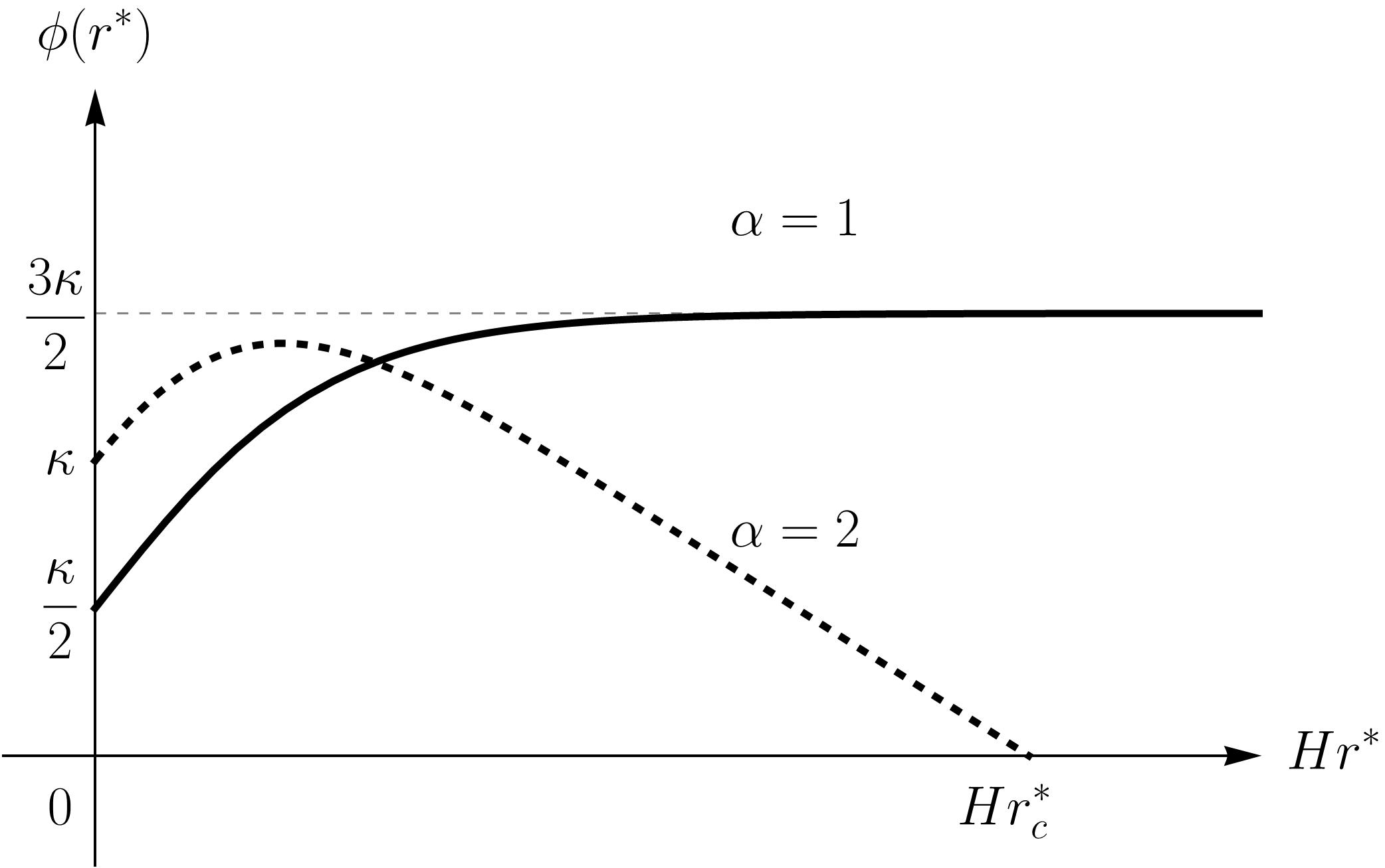
Figure 1: The dilaton solution (34) is plotted in the case of $\alpha=1$ and $\alpha=2$, where $\tilde{\alpha}=\kappa$ is chosen for simplicity. Note that the solid and dashed curves are dilaton fields for the Bunch-Davies vacuum state ($\alpha=1$) and for the quantum state ($\alpha=2$), respectively. The two curves start with positive values of $\kappa/2$ and $\kappa$ at $r^{*}=0$. The solid curve converges to a positive and finite value as $r^{*}\to\infty$ whereas the dashed curve approaches zero at $r^{*}=r^{*}_{c}$.

We are now in a position to calculate the proper temperature. By using the proper energy density (9), the modified Stefan-Boltzmann law (11), and the stress tensor (37), the proper temperature for an arbitrary $\alpha$ is calculated as

$$T=\sqrt{\alpha-1}\left(\frac{T_{\rm GH}}{\sqrt{g}}\right),$$ (40)

where $\alpha\geq 1$ for a real temperature. For $\alpha=1$ corresponding to the Bunch-Davies vacuum (7), the proper temperature vanishes like Eq. (13). In case of $\alpha>1$, the redshift factor in the proper temperature (40) indicates inhomogeneity of the proper temperature due to the breaking of de Sitter symmetry except the time-like Killing symmetry implemented by $\xi^{\mu}_{(t)}\partial_{\mu}=\partial_{t}$.

For the dilaton solution (34), the parameters are shown to satisfy $0<\alpha\leq 1$ and $\tilde{\alpha}>-(\kappa\alpha)/2$ upon requiring the singularity free condition of the dilaton field. In the special case of $\alpha=2$ of interest, the dilaton field goes to zero at a finite $r^{*}$, so a naked singularity occurs as seen in Fig. 1. Thus, both the reality condition for the proper temperature (40) and the singularity free condition for the dilaton field determines $\alpha=1$ uniquely. As a result, the de Sitter invariant Bunch-Davies vacuum is the only well-defined vacuum in thermal equilibrium and the proper temperature globally vanishes in the semiclassical Jackiw-Teitelboim model.

On the other hand, the JT action (17) with the replacement of $H\to i\ell^{-1}$ can describe anti-de Sitter (AdS₂) space ($\ell$ : AdS radius), one might wonder how solutions in the case of AdS₂ space are related to our solutions (33) and (34) in de Sitter (dS₂) space. In AdS₂ space, it has been known that the dilaton solution $\phi_{\rm AdS}$ diverges at its boundary Almheiri:2014cka ; Engelsoy:2016xyb . On the contrary, as seen in Fig. 1, the dilaton solution (34) in dS₂ space approaches a finite value at the boundary ($r^{*}\to\infty$). In fact, a clue to the different behavior of the dilaton solution in AdS₂ and dS₂ space at each boundaries might be found in the dilaton solution in the generalized models Anninos:2017hhn ; Grumiller:2021cwg . In these models, the solutions ($e.g.$, $e^{2\rho}$ and $\phi$) were turned out to interpolate between AdS₂ and dS₂ space. This fact was clearly shown by the scalar curvature which approaches either a negative or a positive constant depending on the large or the small value of dilaton field.

In the CGHS and RST models Callan:1992rs ; Russo:1992ax , the net flux is always zero in thermal equilibrium with equal incoming and outgoing fluxes. The Hartle-Hawking vacuum state is defined as the state annihilated by the annihilation operators that multiply the positive frequency modes for both incoming modes in the past horizon and outgoing modes in the future horizon. It simply means that there are no incoming and outgoing particles at the horizon. Despite the absence of excited particles at the horizon, there exist incoming and outgoing fluxes at infinity because they originates from a macroscopic distance far from the horizon. This interpretation initiated by Unruh Unruh:1977ga is of relevance to the so-called “quantum atmosphere” recently elaborated by Giddings Giddings:2015uzr . In the limit of asymptotic infinity, these incoming and outgoing fluxes are responsible for the Hawking temperature.

Let us now point out some differences between the Gibbons-Hawking temperature and the present proper temperature within the same stress tensor approach in order to compare them evenly. We define the stress tensor (30) in terms of the bulk stress tensor and the boundary stress tensor, respectively as $\langle T_{\pm\pm}\rangle=\langle T_{\pm\pm}^{\rm bulk}\rangle+\langle T_{\pm\pm}^{\rm bdy}\rangle,$ where $\langle T_{\pm\pm}^{\rm bulk}\rangle=(-\kappa/\pi)\left[\left(\partial_{\pm}\rho\right)^{2}-\partial_{\pm}^{2}\rho\right]$ and $\langle T_{\pm\pm}^{\rm bdy}\rangle=(-\kappa/\pi)t_{\pm}(\sigma^{\pm})$. From the boundary stress tensor in the Bunch-Davies vacuum state, we get $\langle T_{\pm\pm}^{\rm bdy}\rangle_{\rm BD}=-(\kappa/\pi)t_{\pm}(\sigma^{\pm})=\kappa H^{2}/(4\pi)$ for $t_{\pm}(\sigma^{\pm})=-H^{2}/4$. In Eq. (14), ignoring the bulk stress tensors, we obtain the Gibbons-Hawking temperature at the origin as $T_{\rm GH}=H/(2\pi)$, which is the same as the result from the detector method where the observer is sitting at the origin Gibbons:1977mu ; Spradlin:2001pw . Note that the boundary stress tensor is nothing but the vacuum expectation value of the normal ordered stress tensor, i.e., $\langle T_{\pm\pm}^{\rm bdy}\rangle=\langle:T_{\pm\pm}:\rangle$, which is not covariant since the normal ordering responsible for a selection of modes is certainly associated with a specific coordinate system doi:10.1142/p378 . In addition, the boundary stress tensor cannot be de Sitter invariant. On the other hand, the stress tensor (30) is true tensor while the boundary stress tensor is anomalous under coordinate transformation. The stress tensor (30) and (31) are compactly written in the de Sitter invariant form of $\langle T_{\mu\nu}\rangle_{\rm BD}=\kappa H^{2}/(2\pi)g_{\mu\nu}$ in the Bunch-Davies state, which results in $\langle T_{\pm\pm}\rangle_{\rm BD}=0$ in the conformal gauge (4). Using Eq. (12), we obtain the vanishing proper temperature.

IV Conclusion and Discussion

In conclusion, the two kinds of the proper temperatures of de Sitter space on the background of two-dimensional de Sitter space warrant particular attention: one is for the de Sitter invariant Bunch-Davies vacuum and the other is for the de Sitter non-invariant state. The proper temperature in the former vacuum globally vanishes whereas the proper temperature in the latter state becomes divergent at the cosmological horizon. The above argument based on the background of de Sitter space was reexamined by employing the two-dimensional dilaton gravity called the semiclassical Jackiw-Teitelboim gravity. Interestingly, the dilaton parameter $\alpha$ can be related to the vacuum condition $t_{\pm}(\sigma)$, so the dilaton configuration determines the state of the stress tensor. For $\alpha=1$, the vacuum state turns out to be the de Sitter invariant Bunch-Davies vacuum: the proper temperature vanishes and the dilaton field is finite. However, in a certain quantum state of $\alpha=2$, the proper temperature is the observer-dependent and a naked dilaton singularity occurs. Consequently, the Bunch-Davies vacuum turns out to be the unique de Sitter invariant vacuum of two-dimensional de Sitter space in equilibrium state and the proper temperature vanishes everywhere.

In fact, the Unruh’s detector method can be applied to de Sitter space Spradlin:2001pw . The thermal property can be deduced from the periodicity of thermal Green function for conformally invariant scalar field propagating on de Sitter space. In the original work by Unruh Unruh:1976db , the observer is in flat space and he or she feels emitted thermal radiation from the accelerated detector absorbing some energy from external accelerator. There is a nice correspondence between Rindler space and de Sitter space. A common feature to a uniformly accelerated observer in Minkowski space and an observer at a fixed distance from the cosmological horizon is that both observers have horizons which prevent them from seeing the whole of the spacetime. Thus, one can expect a similar thermal interpretation in de Sitter space. However, as compered to the Gibbons-Hawking temperature resorting to the detector method where the observer is sitting at the origin in static coordinate system, our investigation for the temperature rests upon the Tolman’s formulation relying on the covariant stress tensor approach. Consequently, the proper temperature called the Tolman temperature was read off from coordinate invariant quantities of the proper energy density and the trace of the stress tensor.

The final comment is in order. In formulating the proper temperature in thermal equilibrium Tolman:1930zza ; Tolman:1930ona , Tolman assumed that the stress tensor should be traceless; in other words, the equation of state should be satisfied. The first law of thermodynamics consists of the proper energy density and the proper pressure, in which one of them should be eliminated by using the equation of state; however, in the presence of trace anomaly, eliminating one quantity leaves the trace term in the first law of thermodynamics. This is the essential reason why the Stefan-Boltzmann law should be modified such as Eq. (11) when the trace of the stress tensor does not vanish Gim:2015era . Quantum-mechanically radiating systems are commonly associated with trace anomalies, so it would be interesting to study what happens in other gravitational systems related to de Sitter space.

References

- (1) A. D. Linde, A New Inflationary Universe Scenario: A Possible Solution of the Horizon, Flatness, Homogeneity, Isotropy and Primordial Monopole Problems, Adv. Ser. Astrophys. Cosmol. 3 (1987) 149–153.
- (2) A. Albrecht and P. J. Steinhardt, Cosmology for Grand Unified Theories with Radiatively Induced Symmetry Breaking, Adv. Ser. Astrophys. Cosmol. 3 (1987) 158–161.
- (3) A. D. Linde, Chaotic Inflation, Phys. Lett. B 129 (1983) 177–181.
- (4) Planck collaboration, P. Ade et al., Planck 2015 results. XX. Constraints on inflation, Astron. Astrophys. 594 (2016) A20, [1502.02114].
- (5) W. Nelson, I. Agullo and A. Ashtekar, Perturbations in loop quantum cosmology, J. Phys. Conf. Ser. 484 (2014) 012069, [1204.1288].
- (6) R. H. Brandenberger, Quantum Field Theory Methods and Inflationary Universe Models, Rev. Mod. Phys. 57 (1985) 1.
- (7) G. Gibbons and S. Hawking, Cosmological Event Horizons, Thermodynamics, and Particle Creation, Phys. Rev. D 15 (1977) 2738–2751.
- (8) R. C. Tolman, On the Weight of Heat and Thermal Equilibrium in General Relativity, Phys. Rev. 35 (1930) 904–924.
- (9) R. Tolman and P. Ehrenfest, Temperature Equilibrium in a Static Gravitational Field, Phys. Rev. 36 (1930) 1791–1798.
- (10) T. Markkanen, De Sitter Stability and Coarse Graining, Eur. Phys. J. C 78 (2018) 97, [1703.06898].
- (11) C. Teitelboim, Gravitation and Hamiltonian Structure in Two Space-Time Dimensions, Phys. Lett. 126B (1983) 41–45.
- (12) R. Jackiw, Lower Dimensional Gravity, Nucl. Phys. B252 (1985) 343–356.
- (13) Y. Gim and W. Kim, A Quantal Tolman Temperature, Eur. Phys. J. C75 (2015) 549, [1508.00312].
- (14) Y. Gim and W. Kim, On the thermodynamic origin of the initial radiation energy density in warm inflation, JCAP 11 (2016) 022, [1608.07466].
- (15) W. G. Unruh, Origin of the Particles in Black Hole Evaporation, Phys. Rev. D 15 (1977) 365–369.
- (16) S. B. Giddings, Hawking radiation, the Stefan–Boltzmann law, and unitarization, Phys. Lett. B 754 (2016) 39–42, [1511.08221].
- (17) M. Eune, Y. Gim and W. Kim, Effective Tolman temperature induced by trace anomaly, Eur. Phys. J. C77 (2017) 244, [1511.09135].
- (18) W. Kim, Origin of Hawking Radiation: Firewall or Atmosphere?, Gen. Rel. Grav. 49 (2017) 15, [1604.00465].
- (19) M. Eune and W. Kim, Proper temperature of the Schwarzschild AdS black hole revisited, Phys. Lett. B773 (2017) 57–61, [1703.00589].
- (20) M. Eune and W. Kim, Test of quantum atmosphere in the dimensionally reduced Schwarzschild black hole, Phys. Lett. B 798 (2019) 135020, [1908.03374].
- (21) P. Davies, S. Fulling, S. Christensen and T. Bunch, Energy Momentum Tensor of a Massless Scalar Quantum Field in a Robertson-Walker Universe, Annals Phys. 109 (1977) 108–142.
- (22) T. S. Bunch and P. C. W. Davies, Quantum field theory in de sitter space: Renormalization by point-splitting, Proceedings of the Royal Society of London. Series A, Mathematical and Physical Sciences 360 (1978) 117–134.
- (23) S. M. Christensen and S. A. Fulling, Trace Anomalies and the Hawking Effect, Phys. Rev. D15 (1977) 2088–2104.
- (24) S. Deser, M. Duff and C. Isham, Nonlocal Conformal Anomalies, Nucl. Phys. B 111 (1976) 45–55.
- (25) M. Spradlin, A. Strominger and A. Volovich, Les Houches lectures on de Sitter space, in Les Houches Summer School: Session 76: Euro Summer School on Unity of Fundamental Physics: Gravity, Gauge Theory and Strings, pp. 423–453, 10, 2001. hep-th/0110007.
- (26) A. M. Polyakov, Quantum Gravity in Two-Dimensions, Mod. Phys. Lett. A2 (1987) 893.
- (27) J. Dowker and R. Critchley, Effective Lagrangian and Energy Momentum Tensor in de Sitter Space, Phys. Rev. D 13 (1976) 3224.
- (28) N. Birrell and P. Davies, Quantum Fields in Curved Space. Cambridge Monographs on Mathematical Physics. Cambridge University Press, 1984.
- (29) R. B. Mann, A. Shiekh and L. Tarasov, Classical and Quantum Properties of Two-dimensional Black Holes, Nucl. Phys. B341 (1990) 134–154.
- (30) T. Muta and S. D. Odintsov, Two-dimensional higher derivative quantum gravity with constant curvature constraint, Prog. Theor. Phys. 90 (1993) 247–255.
- (31) J. P. Lemos, Thermodynamics of the two-dimensional black hole in the Teitelboim-Jackiw theory, Phys. Rev. D54 (1996) 6206–6212, [gr-qc/9608016].
- (32) D. Grumiller, R. McNees and J. Salzer, Cosmological constant as confining U(1) charge in two-dimensional dilaton gravity, Phys. Rev. D 90 (2014) 044032, [1406.7007].
- (33) M. Cvetič and I. Papadimitriou, AdS2 holographic dictionary, JHEP 12 (2016) 008, [1608.07018].
- (34) A. Kitaev and S. J. Suh, The soft mode in the Sachdev-Ye-Kitaev model and its gravity dual, JHEP 05 (2018) 183, [1711.08467].
- (35) A. Almheiri, T. Hartman, J. Maldacena, E. Shaghoulian and A. Tajdini, Replica Wormholes and the Entropy of Hawking Radiation, JHEP 05 (2020) 013, [1911.12333].
- (36) D. Momeni, Real classical geometry with arbitrary deficit parameter(s) in deformed Jackiw–Teitelboim gravity, Eur. Phys. J. C 81 (2021) 202, [2010.00377].
- (37) A. Almheiri and J. Polchinski, Models of AdS2 backreaction and holography, JHEP 11 (2015) 014, [1402.6334].
- (38) J. Engelsöy, T. G. Mertens and H. Verlinde, An investigation of AdS2 backreaction and holography, JHEP 07 (2016) 139, [1606.03438].
- (39) D. Anninos and D. M. Hofman, Infrared Realization of dS2 in AdS2, Class. Quant. Grav. 35 (2018) 085003, [1703.04622].
- (40) D. Grumiller, R. Ruzziconi and C. Zwikel, Generalized dilaton gravity in 2d, SciPost Phys. 12 (2022) 032, [2109.03266].
- (41) C. G. Callan, Jr., S. B. Giddings, J. A. Harvey and A. Strominger, Evanescent black holes, Phys. Rev. D45 (1992) R1005, [hep-th/9111056].
- (42) J. G. Russo, L. Susskind and L. Thorlacius, The Endpoint of Hawking radiation, Phys. Rev. D 46 (1992) 3444–3449, [hep-th/9206070].
- (43) A. Fabbri and J. Navarro-Salas, Modeling Black Hole Evaporation. PUBLISHED BY IMPERIAL COLLEGE PRESS AND DISTRIBUTED BY WORLD SCIENTIFIC PUBLISHING CO., 2005. 10.1142/p378.
- (44) W. G. Unruh, Notes on black hole evaporation, Phys. Rev. D14 (1976) 870.