Optimal probes for continuous variable quantum illumination

Abstract

Quantum illumination is the task of determining the presence of an object in a noisy environment. We determine the optimal continuous variable states for quantum illumination in the limit of zero object reflectivity. We prove that the optimal single mode state is a coherent state, while the optimal two mode state is the two-mode squeezed-vacuum state. We find that these probes are not optimal at non-zero reflectivity, but remain near optimal. This demonstrates the viability of the continuous variable platform for an experimentally accessible, near optimal quantum illumination implementation.

I Introduction

Quantum illumination (QI) was introduced by Lloyd (2008) for discrete-variable states, showing how entangled photonic probes can be utilized to determine the presence of a weakly reflecting object in a region filled with background noise. This scheme was extended to continuous-variable states by Tan et al. (2008), who showed that two-mode Gaussian entangled states outperform single-mode coherent ones. The advantage that entanglement offers in this task has been also discussed in various other works Shapiro and Lloyd (2009); Zhuang et al. (2017); Zhang et al. (2014); Nair and Gu (2020); Las Heras et al. (2017); Shapiro (2009), which has in turn inspired a great deal of experimental research Zhang et al. (2015); Lopaeva et al. (2013); England et al. (2019); Aguilar et al. (2019); Zhang et al. (2013). Of particular interest is recent research into microwave QI Barzanjeh et al. (2015); Xiong et al. (2017); Barzanjeh et al. (2020); Luong et al. (2019, 2018), as at microwave frequencies background radiation naturally contains many photons which are not present at optical frequencies. This is because the bright thermal background is the region where the advantages of QI are more pronounced.

In order to fully exploit the benefits quantum mechanics has to offer for illumination it is essential to know which states are optimal. In the discrete-variable case, the optimal probe states to minimise the probability of error for QI are known Yung et al. (2018), but the same problem for the continuous-variable case has remained unsolved. In this paper, we investigate the optimal probe for QI in the limit of zero object reflectivity. We prove that the coherent state and two-mode squeezed vacuum (TMSV) state are the optimal probes depending on whether entanglement is allowed or not. We also show that for all reflectivities, the optimal probe in the two mode case always has the same form, a Schmidt decomposition in the Fock basis. This greatly simplifies the task of numerically finding the optimal probe state. We find that the numerically optimized non-Gaussian state offer a very limited advantage over Gaussian states. Because Gaussian states can be easily generated in laboratories, these results suggest that producing the optimal probe for QI is much easier in continuous-variable compared to discrete-variable systems.

II Problem formulation

QI is the task where a probe state $\rho_{\text{pr}}$ is used to detect the presence of a reflective object, masked by a noisy environment $\rho_{\text{env}}$, by performing measurements on the received state. We represent the environment as a state diagonal in the Fock basis

$$\rho_{\text{env}}=\sum_{m}\lambda_{m}\outerproduct{m}{m}\,.$$ (1)

We consider two cases: (i) $\rho_{\text{pr}}$ is a single-mode state, and (ii) $\rho_{\text{pr}}$ is a two-mode state. For the case of a two-mode probe, we call one mode the signal which is sent to the region which may contain the object, and the other mode the idler which is reserved for detection purposes (see Fig. 1). The reflective object is modelled as a beam-splitter of reflectivity $r$, through which the environment couples into the system. When the object is present the signal interacts with the object through the beam-splitter operation $U_{\text{bs}}(r)$ and the received state is then

$$\rho_{1}=\tr_{\text{env}}\left[U_{\text{bs}}(r)(\rho_{\text{pr}}\otimes\rho_{\text{env}})U_{\text{bs}}^{{\dagger}}(r)\right]\,.$$ (2)

Here,

$$U_{\text{bs}}(r)=\exp\left[\theta(r)(\hat{a}^{\dagger}\hat{b}-\hat{a}\hat{b}^{\dagger})\right]\,$$ (3)

is the beam-splitter operator with reflection coefficient $r=\text{sin }\theta$, $\hat{a}$ and $\hat{b}$ are the annihilation operators for the signal and environment mode, and $\tr_{\text{env}}$ denotes partial trace over the mode that is lost to the environment. When the object is absent, the reflection coefficient $r$ is set to zero and the received state is $\rho_{0}=\rho_{\text{idler}}\otimes\rho_{\text{env}}$. Our task is to discriminate between the two states $\rho_{0}$ and $\rho_{1}$ as accurately as possible. We assume that we have no prior knowledge about the presence or absence of the object. We do not place any restrictions on the detector and only consider the theoretical bounds that can be achieved using the best possible receiver.

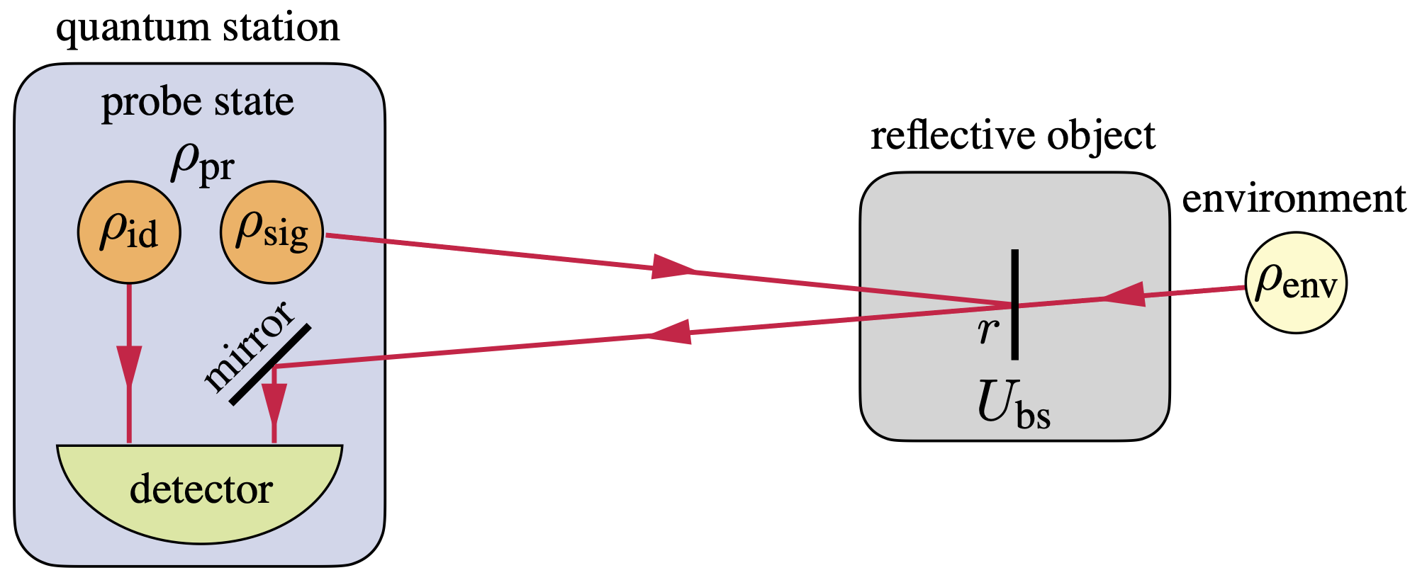
Figure 1: Schematic for quantum illumination. The partially reflective object, modelled as a beam-splitter with reflectivity $r$, is located in a noisy environment represented as a state $\rho_{\text{env}}$ entering the beam-splitter. The signal state $\rho_{\text{sig}}$ mixes with the noisy environment and is reflected to the detector. For two-mode QI the signal $\rho_{\text{sig}}$ and idler $\rho_{\text{id}}$ are entangled and for single-mode QI they are not.

Suppose a single measurement is made to determine what the received state is, then the minimum error probability in distinguishing the two states is given by the Helstrom bound Helstrom (1969)

$$p_{\text{err}}=\frac{1-\frac{1}{2}\left\lVert\rho_{0}-\rho_{1}\right\rVert_{1}}{2}\,,$$ (4)

where $\left\lVert A\right\rVert_{1}$ is the trace norm of the matrix $A$, and we have assumed a uniform prior. If instead, we have $M$ copies of the probe state $\rho_{\text{pr}}$, the probability of error for discriminating between $\rho_{0}^{\otimes M}$ and $\rho_{1}^{\otimes M}$ for large $M$ is given by the quantum Chernoff bound Audenaert et al. (2007); Nussbaum and Szkoła (2009)

$$p_{\text{err}}(M)\approx\kappa^{M}\,,\quad\text{with}\quad\kappa=\min_{0\leqslant s\leqslant 1}\tr\left(\rho_{1}^{s}\rho_{0}^{1-s}\right)\,.$$ (5)

Our aim is to find the optimal probe state for both single-mode and two-mode QI that minimizes the quantum Chernoff bound subject to the constraint that the mean photon number of the probe equals to $n_{\text{pr}}$. This constraint is necessary to avoid probe states with unbounded energy.

Both the Helstrom bound and the quantum Chernoff bound are concave functions of $\rho_{\text{pr}}$, and the domain in which we optimize over is a convex space because density matrices form a convex set. Thus, based on Bauer’s maximum principle Bauer (1958), the optimal probes are obtained at extremal points, i.e., pure states. Unfortunately, this problem is in general quite challenging  Pardalos and Vavasis (1991); Sahni (1974). However, in the region of interest for QI—the low reflectivity limit—we are able to simplify the problem and obtain analytic results. This limit is particularly relevant because this is where QI promises to be most beneficial. This is also the operating regime for microwave illumination where most of the signal is lost.

III Low reflectivity approximation

When the object reflectivity $r$ is low, the state detected is similar to the environment leading to a high probability of error. In this case, we can consider the approximation

$$\rho_{1}\approx\rho_{0}+r\Delta\rho\,,$$ (6)

where $\Delta\rho=\partial\rho_{1}/\partial r$ evaluated at $r=0$. Under this approximation, the Helstrom bound becomes

$$p_{\text{err}}\approx\frac{1-r\,\left\lVert\Delta\rho\right\rVert_{1}}{2}\,.$$ (7)

The quantum Chernoff bound for discriminating the two states $\rho_{0}$ and $\rho_{1}=\rho_{0}+r\Delta\rho$ for small $r$ is $\kappa^{M}$ with

$$\kappa\approx 1-\frac{r^{2}}{2}\sum_{jk}\frac{\left|\bra{\phi_{j}}\Delta\rho\ket{\phi_{k}}\right|^{2}}{(\sqrt{\lambda_{j}}+\sqrt{\lambda_{k}})^{2}}\,,$$ (8)

where $\ket{\phi_{j}}$ are the eigenvectors of $\rho_{0}$ with corresponding eigenvalues $\lambda_{j}$ Audenaert et al. (2007). To calculate $\Delta\rho$, we approximate the beam-splitter operation [see Eq. (3)] for a small reflectivity, using the approximation $\theta\approx r$, i.e.,

$$U_{\text{bs}}(r)\approx 1+r(\hat{a}^{\dagger}\hat{b}-\hat{a}\hat{b}^{\dagger})\,.$$ (9)

Thus, for small $r$, we have

$$U_{\text{bs}}(r)\ket{n,m}\approx\Big{(}\ket{n,m}+\ket{n+1,m-1}r\sqrt{(n+1)m}\\ -\ket{n-1,m+1}r\sqrt{n(m+1)}\Big{)}\,,$$ (10)

where $\ket{n,m}$ represents the Fock state with $n$ and $m$ photons in each mode.

IV Optimal single-mode QI

With this approximation, and a pure probe state $\rho_{\text{pr}}=\outerproduct{\psi}{\psi}$ with

$$\ket{\psi}=\sum_{n}c_{n}\ket{n}\,,$$ (11)

the derivative $\Delta\rho$ becomes

$$\Delta\rho=\sum_{m}\sqrt{m+1}\left(\lambda_{m+1}-\lambda_{m}\right)\\ \times\big{(}\gamma\outerproduct{m+1}{m}+\gamma^{*}\outerproduct{m}{m+1}\big{)}\,,$$ (12)

where

$$\gamma=\sum_{n}c_{n+1}c_{n}^{*}\sqrt{n+1}\,.$$ (13)

Since $\Delta\rho$ only depends on the probe state through $\gamma$, to find the optimal probe state we just have to find the state that maximizes $|\gamma|$. The same probe will minimize both the single measurement and multiple-measurement error probabilities. The optimization result is stated in the following theorem.

Theorem 1.

The single mode state subject to an energy constraint $n_{\text{pr}}$ that maximizes $|\gamma|$ is the coherent state $\ket{\alpha}=\sum_{n}c_{n}\ket{n}$, where

$$c_{n}=e^{-|\alpha|^{2}/2}\frac{\alpha^{n}}{\sqrt{n!}}\,,$$ (14)

with $\alpha=\sqrt{n_{\text{pr}}}$. This is also the probe state that minimizes the Helstrom bound and quantum Chernoff bound in the limit of zero object reflectivity.

Proof (Theorem 1). Since $\gamma=\sum_{n}c_{n+1}c^{*}_{n}\sqrt{n+1}\leqslant\sum_{n}|c_{n+1}||c^{*}_{n}|\sqrt{n+1}$, we can restrict ourselves to the case in which all $c_{n}$ are real. The task is then to maximize

$$\gamma=\sum_{n}c_{n+1}c_{n}\sqrt{n+1}\,,$$ (15)

subject to the normalization and energy constraints

$$\sum_{n}c_{n}^{2}=1\,,\text{ and }\;\sum_{n}n\,c_{n}^{2}=n_{\text{pr}}\,.$$ (16)

Using the method of Lagrange multipliers the necessary condition for the maximum is

$$c_{n+1}\sqrt{n+1}+c_{n-1}\sqrt{n}+2c_{n}(\mu_{1}+n\mu_{2})=0\,,$$ (17)

where $\mu_{1}$ and $\mu_{2}$ are the two Lagrange multipliers. Next, we show that the coherent state satisfies these set of equations. Substituting in Eq. (14), we get

$$\frac{\alpha^{n+1}\sqrt{n+1}}{\sqrt{(n+1)!}}+\frac{\alpha^{n-1}\sqrt{n}}{\sqrt{(n-1)!}}+\frac{2\alpha^{n}(\mu_{1}+n\mu_{2})}{\sqrt{n!}}=0$$

$$\Rightarrow\alpha+\frac{n}{\alpha}+2(\mu_{1}+n\mu_{2})=0\,,$$ (18)

which is satisfied by choosing $\mu_{1}=-\alpha/2$ and $\mu_{2}=-1/2\alpha$. Hence a coherent state is a solution, and all that is left to do is choose $\alpha=\sqrt{n_{\text{pr}}}$ such that it satisfies the energy constraint.   

We note that since $\gamma$ does not depend on the environment, the coherent state will be optimal for any environment that is diagonal in the Fock basis. In particular, when the environment is a thermal state with mean photon number $n_{\text{env}}$, so that the coefficients $\lambda_{m}$ in Eq. (2) reads $\lambda_{m}=n_{\text{env}}^{m}/(1+n_{\text{env}})^{m+1}$, the quantum Chernoff bound for single-mode QI with a coherent state probe has

$$\kappa_{\text{c}}=1-\frac{r^{2}n_{\text{pr}}\left(1+n_{\text{env}}\right)}{\left[1+n_{\text{env}}+\sqrt{n_{\text{env}}(1+n_{\text{env}})}\right]^{2}}\,,$$ (19)

which is consistent with Ref. Tan et al. (2008).

V Optimal two-mode QI

Let us now consider the case where the probe $\rho_{\text{pr}}$ is a two-mode state. The optimal probe in this case can be expressed in the form (see Supplementary material sup for details)

$$\ket{\psi}=\sum_{n}c_{n}\ket{n,n}\,,$$ (20)

which is the Schmidt decomposition in the Fock basis (see also Ref. Sharma et al. (2018)). The fact that the optimal probe state can always be written in this form, regardless of object reflectivity, greatly simplifies the task of numerically finding the optimal probe. Describing the environment in the Fock basis, in the same way as for single-mode QI, we detect the following state when the object is absent

$$\rho_{0}=\sum_{m}\lambda_{m}\outerproduct{m}{m}\otimes\sum_{n}c_{n}^{2}\outerproduct{n}{n}\,.$$ (21)

Utilizing the approximations in Eqs. (6) and (10), $\Delta\rho$ in two-mode QI becomes

$$\Delta\rho=\sum_{nm}\sqrt{m+1}\sqrt{n+1}(\lambda_{m+1}-\lambda_{m})c_{n}c_{n+1}\\ {\times}\Big{(}\outerproduct{m+1,n+1}{m,n}+\outerproduct{m,n}{m+1,n+1}\Big{)}.$$ (22)

Unlike the single-mode QI case, $\Delta\rho$ cannot be written as a sum involving the environment multiplied by a sum involving the probe. Thus, in general, the optimal probe for two-mode QI depends on the environment. In what follows, we restrict to the case with a thermal environment. In the limit of infinite copies of the state, the TMSV state is the optimal state that minimizes the error probability. This result is summarized in the following theorem.

Theorem 2.

In the limit of zero object reflectivity, the two-mode probe for QI in a thermal environment that maximizes the quantum Chernoff bound subject to a constraint on the probe mean photon number of $n_{\text{pr}}$ is the TMSV state $\ket{\psi}=\sum_{n}c_{n}\ket{n,n}$ where $c_{n}=\sqrt{n_{\text{pr}}^{n}/(n_{\text{pr}}+1)^{n+1}}$.

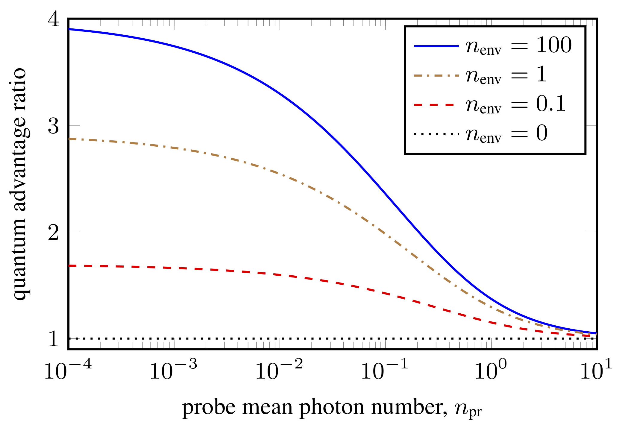
Figure 2: Performance comparison between the optimal two-mode and single-mode probes for QI in the limit of zero object reflectivity. The quantum advantage ratio determines the multiple of additional copies required for the single-mode probe to have the same error performance as the two-mode probe. This has a maximum value of $4$ when the thermal environment has a high mean photon number $n_{\text{env}}$. When $n_{\text{env}}=0$, there is no advantage to using a two-mode probe.

To prove theorem 2, we require the following lemma, (see Lemma 1 of the Supplemental Material sup for prood).

Lemma 1.

Let $G$ be the function

$$G=\sum_{n}(n+1)\mathcal{M}(c_{n}^{2},kc_{n+1}^{2})\,,$$ (23)

where $\mathcal{M}(x,y)$ is a mean function  and $k$ is a positive constant. Then, with the constraints

$$\sum_{n}c_{n}^{2}=1\,,\text{ and }\;\sum_{n}n\,c_{n}^{2}=\bar{n}\,,$$ (24)

$G$ is locally maximized when $c_{n}^{2}=\bar{n}^{n}/(\bar{n}+1)^{n+1}$. If $\mathcal{M}(x,y)$ is concave it is also globally optimal.

Proof (Theorem 2). From Eqs. (8), (21) and (22), simple algebra shows that the quantum Chernoff bound for the state $\ket{\psi}_{\text{TMSV}}$ and a thermal environment with mean photon number $n_{\text{env}}$ has

$$\kappa_{\text{q}}=1-\frac{r^{2}}{4n_{\text{env}}}G\,,$$ (25)

where

$$G=\sum_{n}(n+1)\mathcal{M}\left(c_{n}^{2},\frac{n_{\text{env}}}{1+n_{\text{env}}}c_{n+1}^{2}\right)\,,$$ (26a)

$$\mathcal{M}(x,y)=\frac{4xy}{\left(\sqrt{x}+\sqrt{y}\right)^{2}}\,.$$ (26b)

It can be easily verified that $\mathcal{M}(x,y)$ satisfies the conditions for being a mean function, and is also concave. Lemma 2 then implies that the TMSV state maximizes $G$, and hence minimizes the quantum Chernoff bound, which completes the proof.  

Substituting the coefficients $c_{n}$ for the TMSV into (25), the Chernoff bound for the TMSV in the limit of small $r$ has

$$\kappa_{\text{q}}=1-\frac{r^{2}n_{\text{pr}}\left(1+n_{\text{env}}\right)}{\left[1+n_{\text{env}}+\sqrt{n_{\text{env}}n_{\text{pr}}\frac{(1+n_{\text{env}})}{1+n_{\text{pr}}}}\right]^{2}}\,.$$ (27)

Unlike the single-mode probe, for the two-mode probe, the optimal state for individual measurement is not the same as the optimal probe for collective measurement. In this case, we find that the TMSV state does not minimize the Helstrom bound. Instead a numerical optimization indicates that there exist a different state that outperforms it.

VI Quantum advantage comparisons

We can now compare the performance of single-mode and two-mode QI schemes. In the limit of small $r$, the quantum advantage ratio

$$\frac{\log\kappa_{\text{q}}}{\log\kappa_{\text{c}}}=\left[\frac{1+n_{\text{env}}+\sqrt{n_{\text{env}}(1+n_{\text{env}})}}{1+n_{\text{env}}+\sqrt{\frac{n_{\text{pr}}n_{\text{env}}(1+n_{\text{env}})}{1+n_{\text{pr}}}}}\right]^{2}\,,$$ (28)

gives the multiple of additional copies required by single-mode QI to achieve the same error probability scaling as two-mode QI. This is plotted in Fig. 2. The figure demonstrates that the quantum advantage is greatest for low probe energies and high environment noise. A maximum advantage of 4 is achieved when $n_{\text{pr}}\to 0$ and $n_{\text{env}}\gg 1$ Tan et al. (2008). As $n_{\text{env}}$ becomes smaller, the maximum quantum advantage, which occurs when $n_{\text{pr}}\to 0$, decreases and until finally there is no quantum advantage when the environment is in the vacuum state Shapiro and Lloyd (2009). When $n_{\text{pr}}\gg 1$, $\kappa_{\text{q}}\to\kappa_{c}$ regardless of $n_{\text{env}}$, and the the coherent state probe performs almost as well as the TMSV probe. In this regime, there is no advantage from using a two-mode probe even when the environment noise is large.

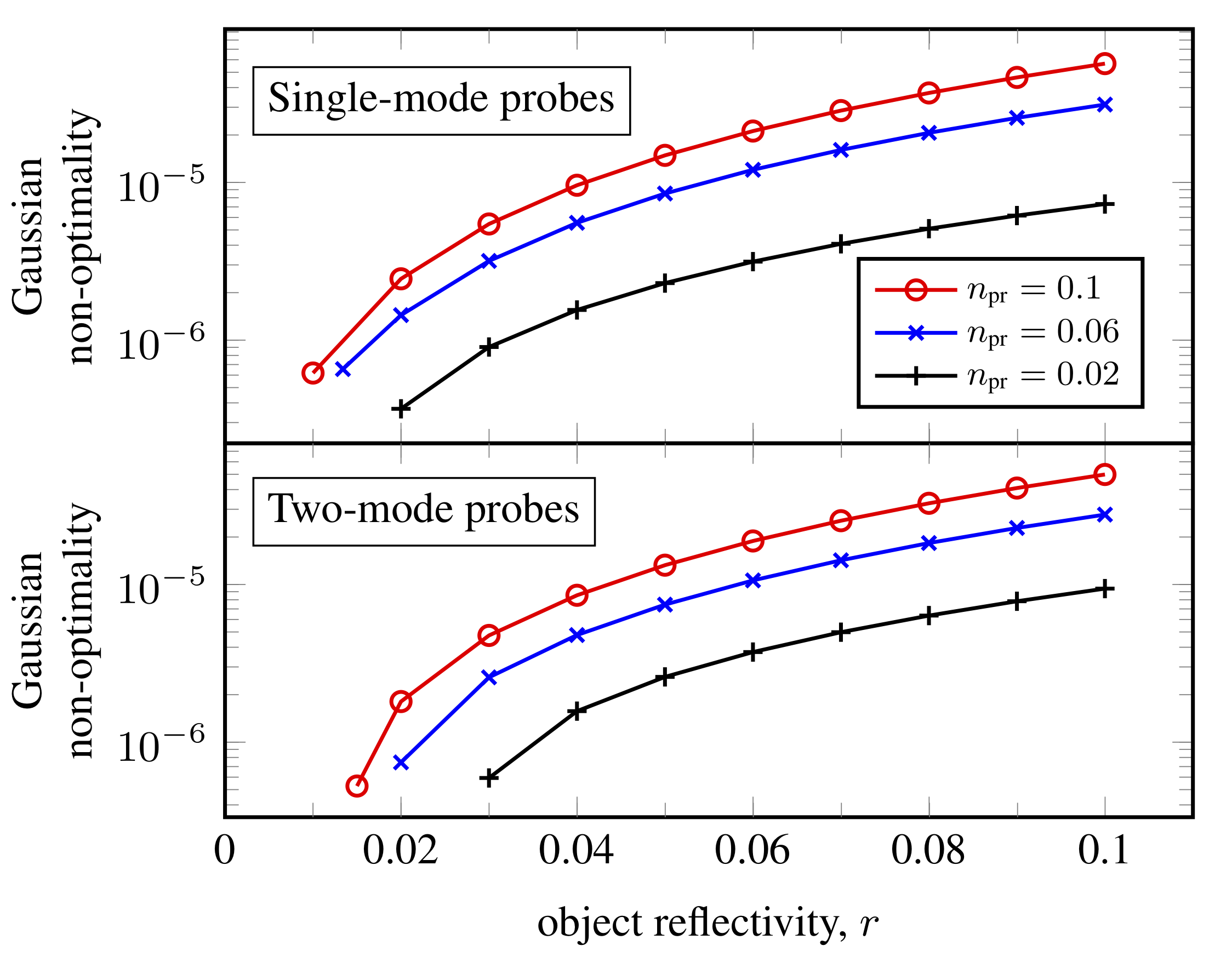
Figure 3: Comparison between the performance of the optimal (non-Gaussian) probe for QI and the Gaussian probe. The top figure shows the single mode Gaussian non-optimality for three different values of $n_{\text{pr}}=0.1$, $0.06$ and $0.02$. The bottom figure shows the same quantity for two mode states. The coherent and squeezed-vacuum probes are only optimal at $r=0$. However, they still remain close to optimal even when $r>0$. The optimal probe states for $r>0$ are non-Gaussian and were computed numerically. The environment mean photon number is set to $n_{\text{env}}=0.5$ in all the simulations.

We have found the optimal states in the limit of zero object reflectivity, but what about for non-zero $r$? It turns out that for non-zero object reflectivity the coherent state and TMSV are no longer the optimal probe states for single-mode and two-mode QI respectively. This is not unexpected since at $r=1$ the problem reduces to discrete-variable illumination with a constraint on the probe energy. But how good are the Gaussian states? To answer this question we compare the coherent state and TMSV state to an optimal state found by numerical optimization . To this end we define the following quantity as the Gaussian non-optimality $1-\log\kappa_{\text{gaus}}/\log\kappa_{\text{opt}}$, where $\kappa_{\text{gaus}}$ is the quantum chernoff exponent for the optimal Gaussian states and $\kappa_{\text{opt}}$ is the quantum chernoff exponent for the numerically optimimised state. The closer this quantity is to zero the closer Gaussian states are to optimal. This is plotted for both single and two mode states in Fig. 3, for a particular choice of environment energy, $n_{\text{env}}=0.5$, and a range of probe energies $n_{\text{pr}}$ between $0.02$ and $0.1$. This shows that the performance of the Gaussian states is close to optimal for small object reflectivities. When the probe mean photon number is small, the Gaussian state will always perform almost as well as the optimal state. This is because as the mean photon number approaches zero, all the states of the given energy look similar, since they are mostly dominated by the zero and one photon number components.

VII Discussion and Conclusions

Our findings complement existing results in the literature where coherent states and TMSV probes were considered, but they were not known or claimed to be optimal Tan et al. (2008); Guha and Erkmen (2009); Lee et al. (2020). For example, our results are consistent with Ref. Nair and Gu (2020) where a lower bound on the probability of error was derived which does not rule out the TMSV being optimal. These results also nicely supplement Ref. De Palma and Borregaard (2018) which showed that the coherent state and the TMSV are optimal in an asymmetric version of continuous-variable QI where the goal is to minimize the probability of a missed detection for a given probability of a false alarm Spedalieri and Braunstein (2014); Wilde et al. (2017).

In this work we proved that in the limit of zero object reflectivity, the coherent state is the optimal probe state for single-mode QI whereas the two-mode squeezed-vacuum state is the optimal two-mode probe. The low reflectivity limit is particularly relevant for microwave QI. We have also demonstrated that these states remain close to optimal for non-zero reflectivities. This result establishes the possibility of continuous-variable states being used as a viable, near-term, close to optimal platform for QI. Future research directions include finding the optimal probe states for non-zero reflectivity and investigating the possible application of multipartite entangled states to QI.

This research is supported by the Australian Research Council (ARC) under the Centre of Excellence for Quantum Computation and Communication Technology (CE110001027), the Singapore Ministry of Education Tier 1 grant MOE2019- T1-002-015, and National Research Foundation Fellowship NRF-NRFF2016-02. We acknowledge funding from the Defence Science and Technology Group.

Appendix A Form of optimal probe two mode quantum illumination

We claim that there exists an optimal probe state for two mode quantum illumination of the form

$$\ket{\psi}=\sum_{n}c_{n}\ket{n,n}\,,$$ (29)

where $c_{n}\geqslant 0$.

Proof. The most general probe state is

$$\ket{\Psi^{\prime}}=\sum_{n}c_{n}\ket{n,\phi_{n}},$$ (30)

where ${\phi_{n}}$ are a set of states that aren’t necessarily orthogonal. $c_{n}$ can be taken to be real since any phase can be absorbed into $\ket{\phi_{n}}$. Let $\rho_{0}$ and $\rho_{1}$ be the possible detected states when the probe is (29) and $\rho^{\prime}_{0}$ and $\rho^{\prime}_{1}$ be the possible detected states when the probe is (30). The existence of a quantum operation which simultaneously transforms $\rho_{0}$ to $\rho^{\prime}_{0}$ and $\rho_{1}$ to $\rho^{\prime}_{1}$ would prove that a probe given by Eq. (29) can perform no worse than a probe given by Eq. (30) proving the theorem. This relies on the assumption that the figure of merit is one such that a quantum operation does not make two states more distinguishable. This is necessarily true of a figure that involves optimisation over measurements, such as probability of error, as any such operation can be included in the measurement. It is also true of the Holevo information, which can be understood because the Holevo information can be obtained by a measurement in the limit of infinite copies of the state.

For a perfectly reflecting object with $r=1$,

$$\rho_{1}=\sum_{n,m}c_{n}c_{m}\ket{n,n}\bra{m,m}\;,$$ (31)

$$\rho^{\prime}_{1}=\sum_{n,m}c_{n}c_{m}\ket{n,\phi_{n}}\bra{m,\phi_{m}}\;,$$ (32)

$$\rho_{0}=\sum_{k}\lambda_{k}\ket{k}\bra{k}\otimes\sum_{m}|c_{m}|^{2}\ket{m}\bra{m}\;,$$ (33)

$$\rho^{\prime}_{0}=\sum_{k}\lambda_{k}\ket{k}\bra{k}\otimes\sum_{m}|c_{m}|^{2}\ket{\phi_{m}}\bra{\phi_{m}}\;,$$ (34)

where $\lambda_{k}$ depends on the number of thermal photons in the environment. We can then do the following quantum operation to transform from $\rho_{0}$ to $\rho^{\prime}_{0}$ and $\rho_{1}$ to $\rho^{\prime}_{1}$:

1. Perform the measurement with POVM elements $\Pi_{0}=I-\Pi_{1}$, $\Pi_{1}=\sum_{n}\ket{n,n}\bra{n,n}$.

2. If the measurement outcome is 1, do a unitary transformation $U$ such that $U\ket{n,n}=\ket{n,\phi_{n}}$ for all n.

3. If the measurement outcome is 0, do the non-unitary operation $O(\ket{n}_{B})=\ket{\phi_{n}}_{B}$.

The measurement in step 1 checks whether there are the same number of photons in mode $A$ and mode $B$. Since this is always true for $\rho_{1}$, measuring $\rho_{1}$ will leave it unchanged and the result will be 1. Measuring $\rho_{0}$ will result in a state with $n=m$ if the measurement result is 1, and $n\neq m$ if the measurement result is 0.

The operation defined in step 2 is unitary since it transforms one set of orthogonal states into another set of orthogonal states. Note that this unitary is not uniquely defined, but this does not matter. Performing this unitary operation on $\rho_{1}$ will transform it to $\rho^{\prime}_{1}$. This unitary also transforms the pure states that make up $\rho_{0}$ for which $n=m$ into the corresponding pure states of $\rho^{\prime}_{0}$.

The measurement outcome of 1 means that the state must have been $\rho_{0}$. The operation defined in step 3 corresponds to measuring the number of photons in mode $B$, and replacing the state with $\phi_{n}$ where $n$ is the number of photons measured. This operation will transform the remaining pure states of $\rho_{0}$ with $n\neq m$ into the corresponding $\rho^{\prime}_{0}$ pure states.

For all other $r$ the beamsplitter operation makes the problem more complicated. Nevertheless we can still find the necessary transformation. The states are

$$\rho_{1}=\sum_{n,m,k}c_{n}c_{m}\lambda_{k}\text{tr}_{\text{env}}\{B(r)\ket{n,k}\bra{m,k}_{AE}B^{\dagger}(r)\}\ket{n}\bra{m}_{B}$$ (35)

$$\rho^{\prime}_{1}=\sum_{n,m,k}c_{n}c_{m}\lambda_{k}\text{tr}_{\text{env}}\{B(r)\ket{n,k}\bra{m,k}_{AE}B^{\dagger}(r)\}\ket{\phi_{n}}\bra{\phi_{m}}_{B}$$ (36)

$$\rho_{0}=\sum_{k}\lambda_{k}\ket{k}\bra{k}\otimes\sum_{m}|c_{m}|^{2}\ket{m}\bra{m}$$ (37)

$$\rho^{\prime}_{0}=\sum_{k}\lambda_{k}\ket{k}\bra{k}\otimes\sum_{m}|c_{m}|^{2}\ket{\phi_{m}}\bra{\phi_{m}}.$$ (38)

The pure states that make up $\rho_{1}$ for $n_{\text{env}}=0$ where $n_{\text{env}}$ is the number of photons in the environment before the beam splitter will be

$$\ket{0,0}_{AB}\ket{0}_{E}+\ket{1,1}_{AB}\ket{0}_{E}+\ket{2,2}_{AB}\ket{0}_{E}+....$$ (39)

$$\ket{0,1}_{AB}\ket{1}_{E}+\ket{1,2}_{AB}\ket{1}_{E}+\ket{2,3}_{AB}\ket{1}_{E}+....$$ (40)

$$\ket{0,2}_{AB}\ket{2}_{E}+\ket{1,3}_{AB}\ket{2}_{E}+\ket{2,4}_{AB}\ket{2}_{E}+....$$ (41)

and so on. For $n_{\text{env}}=1$ we have

$$\ket{1,0}_{AB}\ket{0}_{E}+\ket{2,1}_{AB}\ket{0}_{E}+\ket{3,2}_{AB}\ket{0}_{E}+....$$ (42)

$$\ket{0,0}_{AB}\ket{1}_{E}+\ket{1,1}_{AB}\ket{1}_{E}+\ket{2,2}_{AB}\ket{1}_{E}+....$$ (43)

$$\ket{0,1}_{AB}\ket{2}_{E}+\ket{1,2}_{AB}\ket{2}_{E}+\ket{2,3}_{AB}\ket{2}_{E}+....$$ (44)

and so on, where the environment component is traced out and each term in the expressions are multiplied by some number which we have neglected because it is irrelevant for the discussion. The pure states that make up $\rho^{\prime}_{1}$ are the same except $\ket{n}_{B}$ is replaced with $\ket{\phi_{B}}$. The important part to note about $\rho_{1}$ is that we can measure the difference between the number of photons in mode $A$ and mode $B$ without disturbing any of the pure states. For example states (39) and (43) have the same number of photons in modes $A$ and $B$, mode $A$ of states (40) and (44) lost one photon to the environment and for state (42) mode $A$ gained one photon from the environment. The POVM elements that make up this measurement are

$$\Pi_{0}=\sum_{n}\ket{n,n}\bra{n,n}\;,$$ (45)

$$\Pi_{k}=\sum_{n}\ket{n+k,n}\bra{n+k,n}\text{ for }k\geq 1\;,$$ (46)

$$\Pi_{-k}=\sum_{n}\ket{n,n+k}\bra{n,n+k}\text{ for }k\geq 1\;,$$ (47)

which form a valid measurement since $\sum_{j=-\infty}^{\infty}\Pi_{j}=I$. If this measurement is done on $\rho_{1}$, we will be left with a mixture of the pure states that have the photon difference corresponding to the measurement outcome. Performing a corresponding unitary operation defined by

$$U_{0}\ket{n,n}=\ket{n,\phi_{n}}\;,$$ (48)

$$U_{k}\ket{n+k,n}=\ket{n+k,\phi_{n}}\text{ for }k\geq 1\;,$$ (49)

$$U_{-k}\ket{n,n+k}=\ket{n,\phi_{n+k}}\text{ for }k\geq 1\;,$$ (50)

converts the pure states of $\rho_{1}$ into the pure states $\rho^{\prime}_{1}$. The quantum operation defined by the measurement and unitary transformations also converts $\rho_{0}$ to $\rho^{\prime}_{0}$. The existence of this operation proves our claim.   

Appendix B Proof of lemma 1

Lemma 2.

The EPR state $\ket{\psi}=\sum_{n}c_{n}\ket{n}\ket{n}$ with $c_{n}=\sqrt{\bar{n}^{n}/(\bar{n}+1)^{n+1}}$, is a local optima for the maximisation of

$$G=\sum_{n}(n+1)\mathcal{M}(c_{n}^{2},gc_{n+1}^{2})\,,$$ (51)

where $\mathcal{M}(x,y)$ is a mean function and $g$ is a positive constant. If $\mathcal{M}(x,y)$ is concave it is globally optimal.

Proof. A mean function $m(x,y)$ is a mean function if it can be written as $m(x,y)=yf(\frac{x}{y})$ where $f$ has the following properties:

1. $f$ is monotone increasing, i.e. $x\geq y$ implies $f(x)\geq f(y)$.

2. $xf(x^{-1})=f(x)$. This ensures $m(x,y)$ is symmetric in $x$ and $y$.

3. $f(1)=1$.

We now use property 2 of a mean function and take the derivative

$$f^{\prime}(x)=f(x^{-1})+xf^{\prime}(x^{-1}).$$ (52)

Since

$$G=\sum_{n=0}^{\infty}(n+1)c_{n+1}^{2}f\left(\frac{c_{n}^{2}}{c_{n+1}^{2}}\right)=\sum_{n=1}^{\infty}nc_{n-1}f\left(\frac{c_{n}^{2}}{c_{n-1}^{2}}\right)\;.$$ (53)

The derivative is

$$\frac{\partial G}{\partial c_{k}}=(k+1)2c_{k}\left(f\left(\frac{c_{k+1}^{2}}{c_{k}^{2}}\right)+\frac{c_{k}^{2}}{c_{k+1}^{2}}f^{\prime}\left(\frac{c_{k+1}^{2}}{c_{k}^{2}}\right)\right)\\ +2kc_{k}\left(f\left(\frac{c_{k-1}^{2}}{c_{k}^{2}}\right)+\frac{c_{k}^{2}}{c_{k-1}^{2}}f^{\prime}\left(\frac{c_{k-1}^{2}}{c_{k}^{2}}\right)\right).$$ (54)

Using the normalisation and energy constraints as we did in the classical case we get the following condition for the optimal point

$$\frac{\partial G}{\partial c_{k}}+2c_{k}\mu_{1}+2c_{k}k\mu_{2}=0,$$ (55)

where $\mu_{1}$ and $\mu_{2}$ are Lagrange multipliers as before. This equation can be satisfied if the term multiplied by $2c_{k}$ equals zero and if the term multiplied by $2c_{k}k$ equals zero, i.e.

$$f\left(\frac{c_{k-1}^{2}}{c_{k}^{2}}\right)+\frac{c_{k}^{2}}{c_{k-1}^{2}}f^{\prime}\left(\frac{c_{k-1}^{2}}{c_{k}^{2}}\right)+\mu_{1}=0$$ (56)

$$f\left(\frac{c_{k+1}^{2}}{c_{k}^{2}}\right)+\frac{c_{k}^{2}}{c_{k+1}^{2}}f^{\prime}\left(\frac{c_{k+1}^{2}}{c_{k}^{2}}\right)+f\left(\frac{c_{k-1}^{2}}{c_{k}^{2}}\right)+\frac{c_{k}^{2}}{c_{k-1}^{2}}f^{\prime}\left(\frac{c_{k-1}^{2}}{c_{k}^{2}}\right)+\mu_{2}=0.$$ (57)

By choosing $c_{k}=\sqrt{\bar{n}^{k}/(\bar{n}+1)^{k+1}}$, the dependency of the above equations on $k$ is removed, hence it is possible to find $\mu_{1}$ and $\mu_{2}$ which satisfy the equations. Thus the two mode squeezed vacuum is optimal.

References

- Lloyd (2008) S. Lloyd, Science 321, 1463 (2008).
- Tan et al. (2008) S.-H. Tan, B. I. Erkmen, V. Giovannetti, S. Guha, S. Lloyd, L. Maccone, S. Pirandola, and J. H. Shapiro, Phys. Rev. Lett. 101, 253601 (2008).
- Shapiro and Lloyd (2009) J. H. Shapiro and S. Lloyd, New J. Phys. 11, 063045 (2009).
- Zhuang et al. (2017) Q. Zhuang, Z. Zhang, and J. H. Shapiro, Phys. Rev. Lett. 118, 040801 (2017).
- Zhang et al. (2014) S. Zhang, X. Zou, J. Shi, J. Guo, and G. Guo, Phys. Rev. A 90, 052308 (2014).
- Nair and Gu (2020) R. Nair and M. Gu, Preprint at arXiv:2002.12252 (2020).
- Las Heras et al. (2017) U. Las Heras, R. Di Candia, K. G. Fedorov, F. Deppe, M. Sanz, and E. Solano, Sci. Rep. 7, 9333 (2017).
- Shapiro (2009) J. H. Shapiro, Phys. Rev. A 80, 022320 (2009).
- Zhang et al. (2015) Z. Zhang, S. Mouradian, F. N. C. Wong, and J. H. Shapiro, Phys. Rev. Lett. 114, 110506 (2015).
- Lopaeva et al. (2013) E. D. Lopaeva, I. Ruo Berchera, I. P. Degiovanni, S. Olivares, G. Brida, and M. Genovese, Phys. Rev. Lett. 110, 153603 (2013).
- England et al. (2019) D. G. England, B. Balaji, and B. J. Sussman, Phys. Rev. A 99, 023828 (2019).
- Aguilar et al. (2019) G. H. Aguilar, M. A. de Souza, R. M. Gomes, J. Thompson, M. Gu, L. C. Céleri, and S. P. Walborn, Phys. Rev. A 99, 053813 (2019).
- Zhang et al. (2013) Z. Zhang, M. Tengner, T. Zhong, F. N. C. Wong, and J. H. Shapiro, Phys. Rev. Lett. 111, 010501 (2013).
- Barzanjeh et al. (2015) S. Barzanjeh, S. Guha, C. Weedbrook, D. Vitali, J. H. Shapiro, and S. Pirandola, Phys. Rev. Lett. 114, 080503 (2015).
- Xiong et al. (2017) B. Xiong, X. Li, X.-Y. Wang, and L. Zhou, Ann. Phys. 385, 757 (2017).
- Barzanjeh et al. (2020) S. Barzanjeh, S. Pirandola, D. Vitali, and J. M. Fink, Sci. Adv. 6 (2020), 10.1126/sciadv.abb0451.
- Luong et al. (2019) D. Luong, C. W. S. Chang, A. M. Vadiraj, A. Damini, C. M. Wilson, and B. Balaji, IEEE Transactions on Aerospace and Electronic Systems , 1 (2019).
- Luong et al. (2018) D. Luong, B. Balaji, C. W. Sandbo Chang, V. M. Ananthapadmanabha Rao, and C. Wilson, in 2018 International Carnahan Conference on Security Technology (ICCST) (2018) pp. 1–5.
- Yung et al. (2018) M.-H. Yung, F. Meng, and M.-J. Zhao, Preprint at arXiv:1801.07591 (2018).
- Helstrom (1969) C. W. Helstrom, J. Stat. Phys. 1, 231 (1969).
- Audenaert et al. (2007) K. M. R. Audenaert, J. Calsamiglia, R. Muñoz Tapia, E. Bagan, L. Masanes, A. Acin, and F. Verstraete, Phys. Rev. Lett. 98, 160501 (2007).
- Nussbaum and Szkoła (2009) M. Nussbaum and A. Szkoła, Ann. Statist. 37, 1040 (2009).
- Bauer (1958) H. Bauer, Archiv der Mathematik 9, 389 (1958).
- Pardalos and Vavasis (1991) P. M. Pardalos and S. A. Vavasis, J. of Global Optim. 1, 15 (1991).
- Sahni (1974) S. Sahni, SIAM J. Comp. 3, 262 (1974).
- (26) See Supplemental Material at link provided for details on the form of the optimal two mode probe (theorem 1) and the proof of lemma 1.
- Sharma et al. (2018) K. Sharma, M. M. Wilde, S. Adhikari, and M. Takeoka, New J. Phys. 20, 063025 (2018).
- Note (1) A mean function is a function that defines an ‘average value’ of two numbers. Familiar examples of mean functions are the arithmetic mean, harmonic mean and geometric mean. A function is a mean function if it can be written as where is: (i) monotone increasing, (ii) so that is symmetric, and (iii) . See for example Refs. Petz (1996); Hiai and Petz (2009).
- Note (2) Numerical optimization was carried out using standard techniques and programmes in MATLAB. The coherent and TMSV states were used as starting points for the density matrices in the single and two mode case respectively. These states were then subject to the operations representing a quantum illumination channel and the subsequent error probabilities were computed using Eq. (5\@@italiccorr). The error probability was then minimised over physical density matrices, subject to the energy constraint, using fmincon. For this reason, the solutions found might correspond to local minima instead of the global minima.
- Guha and Erkmen (2009) S. Guha and B. I. Erkmen, Phys. Rev. A 80, 052310 (2009).
- Lee et al. (2020) S.-Y. Lee, Y. S. Ihn, and Z. Kim, Preprint at arXiv:2004.09234 (2020).
- De Palma and Borregaard (2018) G. De Palma and J. Borregaard, Phys. Rev. A 98, 012101 (2018).
- Spedalieri and Braunstein (2014) G. Spedalieri and S. L. Braunstein, Phys. Rev. A 90, 052307 (2014).
- Wilde et al. (2017) M. M. Wilde, M. Tomamichel, S. Lloyd, and M. Berta, Phys. Rev. Lett. 119, 120501 (2017).
- Petz (1996) D. Petz, Linear Algebra and its Applications 244, 81 (1996).
- Hiai and Petz (2009) F. Hiai and D. Petz, Linear Algebra and its Applications 430, 3105 (2009).