Musings about Constructions of Efficient Latin Hypercube Designs with Flexible Run-sizes

Abstract

Efficient Latin hypercube designs (LHDs), including maximin distance LHDs, maximum projection LHDs and orthogonal LHDs, are widely used in computer experiments. It is challenging to construct such designs with flexible sizes, especially for large ones. In the current literature, various algebraic methods and search algorithms have been proposed for identifying efficient LHDs, each having its own pros and cons. In this paper, we review, summarize and compare some currently popular methods aiming to provide guidance for experimenters on what method should be used in practice. Using the R package we developed which integrates and improves various algebraic and searching methods, many of the designs found in this paper are better than the existing ones. They are easy to use for practitioners and can serve as benchmarks for the future developments on LHDs.

Keywords: Simulated Annealing; Particle Swarm Optimization; Genetic Algorithm; Space-filling design; Orthogonality; Maximum projection design.

1 Introduction

Computer experiments are widely used in both scientific researches and industrial productions to simulate the real-world problems with complex computer codes (Sacks et al., 1989; Fang et al., 2005). Different from physical experiments, computer experiments are deterministic and free from random errors, and hence replications should be avoided (Santner et al., 2003). The most popular experimental designs for computer experiments are Latin hypercube designs (LHDs, McKay et al. (1979)), which has uniform one-dimensional projections and avoids replications on every dimension. According to practical needs, there are various types of efficient LHDs (aka. optimal LHDs), including space-filling LHDs, maximum projection LHDs and orthogonal LHDs. There is a rich literature on how to construct such designs, but it is still very challenging to find efficient ones for moderate or large design sizes (Ye, 1998; Fang et al., 2005; Joseph et al., 2015; Xiao and Xu, 2018).

An LHD with $n$ runs and $k$ factors is an $n\times k$ matrix with each column being a random permutation of $1,\ldots,n$. Throughout this paper, $n$ denotes the run size and $k$ denotes the number of factors. A space-filling LHD has its sampled region as scattered-out as possible and its unsampled region as minimal as possible, which considers the uniformity of all dimensions. Different criteria were proposed to measure designs’ space-filling property, including the maximin and minimax distance criteria (Johnson et al., 1990; Morris and Mitchell, 1995), the discrepancy criteria (Hickernell, 1998; Fang et al., 2002, 2005) and the entropy criterion (Fang et al., 2002). Since there are as many as $(n!)^{k-1}$ candidate LHDs for a given design size, it is nearly impossible to find the space-filling one via enumeration when $n$ and $k$ are moderate or large. In the current literature, both the search algorithms (Morris and Mitchell, 1995; Leary et al., 2003; Joseph and Hung, 2008; Ba et al., 2015; Ye et al., 2000; Jin et al., 2005; Liefvendahl and Stocki, 2006; Grosso et al., 2009; Chen et al., 2013) and algebraic constructions (Zhou and Xu, 2015; Xiao and Xu, 2017; Wang et al., 2018) are used to identify space-filling LHDs.

The search algorithms can lead to space-filling LHDs with flexible sizes. Specifically, Morris and Mitchell (1995) proposed a simulated annealing (SA) algorithm which can avoid being trapped at local optima and find the global best design. Following their work as well as that of Tang (1993), Leary et al. (2003) proposed to construct orthogonal array-based LHDs (OALHDs) using the SA algorithm. Joseph and Hung (2008) proposed a multi-objective criterion and developed an adapted SA algorithm, which considers both the orthogonality and the space-filling property. Ba et al. (2015) extended the work of sliced Latin hypercube designs (SLHD, Qian (2012)) and proposed a two-stage SA algorithm. In addition to these SA based algorithms, there are various other search algorithms for efficient designs. Ye et al. (2000) proposed the columnwise pairwise (CP) algorithm to search for efficient symmetric LHDs. Jin et al. (2005) proposed the enhanced stochastic evolutionary algorithm (ESE), which is a combination of exchange procedure (inner loop) and threshold determination (outer loop). Liefvendahl and Stocki (2006) proposed to use genetic algorithm (GA), and implemented a strategy that focused on the global best directly during the search process. Grosso et al. (2009) proposed to use Iterated Local Search heuristics where local searching and perturbation are considered. Chen et al. (2013) proposed a version of particle swarm optimization (PSO) algorithm whose search process is to gradually reduce the Hamming distances between each particle and global best (or personal best) via exchanging elements. Generally speaking, the search algorithms are often computationally expensive for even moderate design sizes. For certain sizes, algebraic constructions can generate efficient LHDs at nearly no cost. For example, Xiao and Xu (2017) adopted Costas’ arrays to obtain space-filling saturate LHDs or Latin squares with run sizes $n=p-2,p-1$ or $p$, where $p$ is any prime power. Wang et al. (2018) proposed to apply the Williams transformation (Williams, 1949) to linearly permuted good lattice point sets to construct maximin LHDs when the factor size is no greater than the number of positive integers that are co-prime to the run size.

Most space-filling designs only consider the uniformity in full-dimensional projections. To guarantee the space-filling properties on all possible dimensions, Joseph et al. (2015) proposed the maximum projection designs. From two to $k-1$ projections, maximum projection LHDs (MaxPro LHDs) are generally more space-filling compared to the maximin distance LHDs. The construction of MaxPro LHDs is also challenging, and Joseph et al. (2015) proposed to use an SA algorithm. In this paper, we further propose a new GA framework that can lead to many better MaxPro LHDs; see Section 5 for examples.

Different from space-filling LHDs which minimize the similarities among rows, orthogonal LHDs (OLHDs) are another popular type of efficient designs which consider the similarities among columns. All search algorithms introduced above can also be used to obtain OLHDs which have zero column-wise correlations. Algebraic constructions are available for certain design sizes. Specifically, Ye (1998) proposed an algebraic construction of OLHDs with run sizes $n=2^{m}+1$ and factor sizes $k=2m-2$ with $m$ being any integer no less than 2, and Cioppa and Lucas (2007) further extended this approach to accommodate more factors. Sun et al. (2010) extended their earlier work (Sun et al., 2009) to construct OLHDs with $n=r2^{c+1}$ or $n=r2^{c+1}+1$ and $k=2^{c}$ where $c$ and $r$ are any two positive integers. Yang and Liu (2012) proposed to use generalized orthogonal designs to construct OLHDs and nearly orthogonal LHDs (NOLHDs) with $n=2^{r+1}$ or $n=2^{r+1}+1$ and $k=2^{r}$ where $r$ is any positive integer. Steinberg and Lin (2006) developed a construction method based on factorial designs and group rotations with $n=2^{2^{m}}$ and $k=2^{m}t$, where $m$ is any positive integer and $t$ is the number of rotation groups. Georgiou and Efthimiou (2014) proposed a construction method based on orthogonal arrays and their full fold-overs with $n=2ak$ runs and $k$ factors, where $k$ is the size of orthogonal matrix and $a$ is any positive integer. Additionally, inheriting the properties of orthogonal arrays, various types of efficient LHDs can be constructed. Tang (1993) proposed to construct OALHDs by deterministically replacing elements from orthogonal arrays, which tend to have better space-filling proprieties with low column-wise correlations. Lin et al. (2009) proposed to use OLHDs or NOLHDs as starting designs and then couple them with orthogonal arrays for constructing OALHDs. Their method requires fewer runs to accommodate large numbers of factors with $n^{2}$ runs and $2fp$ factors, where $n$ and $p$ are designs sizes of the OLHDs or NOLHDs and $2f$ is the number of columns in the coupled orthogonal array. Butler (2001) implemented the Williams transformation (Williams, 1949) to construct OLHDs under a second-order cosine model with $n$ being odd primes and $k\leq n-1$.

We developed an R package named LHD available on the Comprehensive R Archive Network (https://cran.r-project.org/web/packages/LHD/index.html), which integrates and improves current popular searching and algebraic methods for constructing maximin distance LHDs, Maxpro LHDs, OLHDs and NOLHDs. With this package, users with little or no background on design theory can easily find efficient LHDs with the required design sizes. In this paper, we summarize and compare different methods to provide guidance for practitioners, and many new designs that are better than the existing ones are discovered by using the developed package.

The rest of the paper is organized as follows. Section 2 illustrates different optimality criteria for LHDs. Section 3 demonstrates the adopted search algorithms. Section 4 discusses some algebraic constructions for certain design sizes. Section 5 provides numerical results and comparisons generated by the developed LHD package. Section 6 concludes with some discussions on the future research. Some examples on the LHD package implementations are available in the Appendix.

2 Optimality Criteria for LHDs

2.1 Maximin distance Criterion

There are various criteria proposed to measure designs’ space-filling properties (Johnson et al., 1990; Hickernell, 1998; Fang et al., 2002). In this paper, we focus on the currently popular maximin distance criterion (Johnson et al., 1990), which seeks to scatter design points over the experimental domains such that the minimum distances between points are maximized. Let X denote an LHD matrix throughout this paper. Define the $L_{q}$-distance between two runs $x_{i}$ and $x_{j}$ of X as $d_{q}(x_{i},x_{j})=\left\{\sum_{k=1}^{m}|x_{ik}-x_{jk}|^{q}\right\}^{1/q}$ where $q$ is an integer. Define the $L_{q}$-distance of design X as $d_{q}(\textbf{X})=\text{min}\{d_{q}(x_{i},x_{j}),1\leq i<j\leq n\}$. In this paper, we consider $q=1$ and $q=2$, i.e. the Manhattan ($L_{1}$) and Euclidean ($L_{2}$) distances. A design X is called a maximin $L_{q}$-distance design if it has the unique largest $d_{q}(\textbf{X})$ value. When more than one designs have the same largest $d_{q}(\textbf{X})$, the maximin distance design sequentially maximizes the next minimum inter-site distances.

To express the maximin distance criterion in a more convenient way, Morris and Mitchell (1995) and Jin et al. (2005) proposed the $\phi_{p}$ criterion which is defined as

$$\phi_{p}=\bigg{\{}\sum_{i=1}^{n-1}\sum_{j=i+1}^{n}d_{q}(x_{i},x_{j})^{-p}\bigg{\}}^{1/p}.$$ (1)

The $\phi_{p}$ criterion in Equation (1) is asymptotically equivalent to the Maximin distance criterion as $p\to\infty$. In practice, $p=15$ often suffices.

2.2 Maximum Projection Criterion

Maximin distance LHDs focus on the space-filling properties in the full dimensional spaces, but their projection properties in the sub-spaces are not guaranteed. Joseph et al. (2015) proposed the maximum projection LHDs that consider designs’ space-filling properties in all possible dimensional spaces. Such designs minimize the maximum projection criterion, which is defined as

$$\mathop{\mathrm{min}}\limits_{\textbf{X}}\psi(\textbf{X})=\Bigg{\{}\frac{1}{{n\choose 2}}\sum_{i=1}^{n-1}\sum_{j=i+1}^{n}\frac{1}{\Pi_{l=1}^{k}(x_{il}-x_{jl})^{2}}\Bigg{\}}^{1/k}.$$ (2)

From Equation (2), we can see that any two design points should be apart from each other in any projection to minimize the value of $\psi(\textbf{X})$. Thus, the maximum projection LHDs consider the space-filling properties in all possible sub-spaces.

2.3 Orthogonality Criteria

Orthogonal and nearly orthogonal designs which aim to minimizing the correlations between factors are widely used in experiments (Georgiou, 2009; Steinberg and Lin, 2006; Sun and Tang, 2017). Two major correlation-based criteria to measure designs’ orthogonality is the average absolute correlation criterion and the maximum absolute correlation criterion (Georgiou, 2009), denoted as ave$(|q|)$ and max$|q|$, respectively:

$$\mathop{\mathrm{ave}}\limits(|q|)=\frac{2\sum_{i=1}^{k-1}\sum_{j=i+1}^{k}|q_{ij}|}{k(k-1)}\text{ and }\mathop{\mathrm{max}}\limits|q|=\mathop{\mathrm{max}}\limits_{i,j}|q_{ij}|,$$ (3)

where $q_{ij}$ is the correlation between the $i$th and $j$th columns of the design matrix X. Orthogonal designs have ave$(|q|)=0$ and max$|q|=0$, which may not exist for all design sizes. Designs with smaller ave$(|q|)$ or max$|q|$ are generally preferred in practice.

3 Search Algorithms for Efficient LHDs with Flexible Sizes

3.1 Simulated Annealing Based Algorithms

The simulated annealing (SA, Kirkpatrick et al. (1983)) is a probabilistic optimization technique, whose name comes from the phenomenon of annealing process in metallurgy. The SA simulates the process of heating a material beyond a critical temperature and then gradually cooling it in a controlled manner in order to minimize its defects. Morris and Mitchell (1995) proposed an SA algorithm for searching maximin distance LHDs with flexible sizes. The algorithm starts with a random LHD and then exchanges two random elements from a randomly chosen column. If this exchange leads to an improvement, the design would be updated and then the algorithm would iteratively proceed to another round of exchange. If the exchange process does not lead to an improvement, the design still has a chance to be updated with a probability controlled by the current temperature (a tuning parameter in the algorithm), which prevents the search process from getting stuck at a local optima. When there are no improvements after certain attempts, the temperature would be annealed to decrease the probability of updating the design matrix. The general framework of SA is summarized in Algorithm 1, where $\Phi$ is the function of the optimality criterion to be minimized.

Algorithm 1 The Simulated Annealing algorithm

1:  Set the tuning parameters: initial temperature $T$, the maximum number of iterations $N$ and the number of consecutive attempts $S$. Set the counter index $C=1$.

2:  Generate a random LHD X.

3:  Randomly choose a column from X.

4:  Exchange two randomly selected elements within the chosen column in the previous step, and denote the new design as $\textbf{X}_{new}$.

5:  If $\Phi(\textbf{X}_{new})<\Phi(\textbf{X})$, then $\textbf{X}=\textbf{X}_{new}$. Otherwise, let $\textbf{X}=\textbf{X}_{new}$ with a probability of $\hbox{exp}[-\frac{\Phi(\textbf{X}_{new})-\Phi(\textbf{X})}{T}]$.

6:  When no improvements are found consecutively for $S$ attempts, decrease the temperature $T$ and repeat Steps 3$-$5.

7:  If $C<N$, set $C=C+1$ and repeat Steps 3$-$6; Otherwise, stop the algorithm.

Based on the SA framework, Leary et al. (2003) proposed to construct orthogonal array-based LHD (OALHD), where they modified the Steps 2 and 4 in Algorithm 1. In Step 2, an OALHD generated by level expansion of an orthogonal array (Tang, 1993) is used as the initial design. In Step 4, two distinct elements from a randomly chosen column in X that share the same entry in the orginal orthogonal array are exchanged to form the new design matrix $\textbf{X}_{new}$. The existence of OALHDs is determined by the existence of the corresponding initial orthogonal arrays.

Joseph and Hung (2008) proposed another modified version of the SA algorithm, which considers both the maximin distance and orthogonality criteria. It chooses the $l^{*}$th column in Step 3, and exchange the $i^{*}$th element with a random one in the $l^{*}$th column to form the new design $\textbf{X}_{new}$ in Step 4, where $l^{*}=\mathop{\mathrm{argmax}}\limits_{l}\rho_{l}^{2}$ ($\rho_{l}^{2}$ is the average pairwise correlation between the $l$th and other columns) and $i^{*}=\mathop{\mathrm{argmax}}\limits_{i}(\sum_{j\neq i}d(x_{i},x_{j})^{-p})^{1/p}$ ($d(x_{i},x_{j})$ is the distance between the $i$th and $j$th row in X). This algorithm leads to efficient LHDs minimizing both $\phi_{p}$ and ave$(|q|)$ criteria, but is computationally heavy, as it needs to calculate all $\rho_{l}^{2}$ values and row-wise distances at each iteration.

Based on the SA framework, Ba et al. (2015) and Qian (2012) proposed to construct space-filling sliced Latin hypercube design (SLHD). An $n$-run SLHD can be partitioned into $t$ slices of sub-matrices ($\textbf{X}=\bigcup_{i=1}^{t}\textbf{X}_{i}$) where each slice $\textbf{X}_{i}$ is also an LHD with $m=n/t$ runs. This algorithm consists of two stages: the first stage aims to optimize the design matrix from the slice perspective via exchanging elements from a random column within a random slice, and the second stage optimizes the design matrix from the element perspective via replacing $t$ of level $l$ ($l=1,\ldots,m$) with a random permutation of $\{(l-1)t+1,\ldots,lt\}$ and then exchanging the two random elements within the permutation. When $t=1$, this algorithm targets on finding the general space-filling LHDs.

3.2 Particle Swarm Optimization Algorithms

Particle swarm optimization (PSO) (Kennedy and Eberhart, 1995) is a meta-heuristic optimization algorithm inspired by social behaviors of animals, e.g. the flying pattern in a bird flock. The PSO optimizes the problem by iteratively trying to improve a candidate solution in terms of a given measure. It solves the problem by having a population of particles (candidate solutions), and moving them around in the searching space according to some mathematical formulae over the particle’s position and velocity. The movement of each particle is affected by its local best known position and is also guided toward the best positions in the searching space, which are updated as better positions found by other particles. Such a strategy is expected to move the swarm toward the best solutions.

Recent researches (Chen et al., 2013, 2015; Wong et al., 2015) adapted the classic PSO algorithm for searching optimal experimental designs, which is a discrete optimization task. Specifically, Chen et al. (2013) proposed a PSO based algorithm, denoted as the LaPSO, to search maximin distance LHDs, which re-defined the steps on how each particle updates its velocity and position in the general PSO framework. It targets on reducing the Hamming distances between each particle and the global best (or corresponding personal best) via exchanging elements deterministically, where the Hamming distance is the total number of positions whose corresponding elements are different between the two LHDs. We summarize this method in Algorithm 2.

In Algorithm 2, the LaPSO first initializes particles with random LHDs, and calculate the personal best and the global best. The exchange process is implemented for each column of each particle via switching the current element with the element whose location is the same as the current one in the global or personal best. Steps 8 and 9 in Algorithm 2 illustrate this exchange process on how to update the position of each particle and move them towards the global and personal best. Note that either Step 8 or 9 can be skipped or repeated, but they cannot be skipped simultaneously. Though there is no hard limit on the number of repetition, a large number, e.g. $2n$, can make every element in the current column nearly the same as the global or personal best. Different from the random exchange in the SA based algorithms, the exchange in the LaPSO connects each particle with the personal best, global best or both. As every exchange step at most reduces the Hamming distance by one, the LaPSO may be computationally cumbersome for large design sizes.

Algorithm 2 The LaPSO Algorithm

1:  Set the maximum number of iterations $N$ and the counter index $C=1$.

2:  Generate $m$ random $n\times k$ LHDs, denoted by $L_{1}^{0},\ldots,L_{m}^{0}$, for $m$ particles.

3:  Initialize the personal best for each particle. Set $\boldsymbol{p_{i}}=L_{i}^{0}$ for $i=1,\ldots,m$.

4:  Initialize the global best $\boldsymbol{g}=\mathop{\mathrm{argmin}}\limits_{i}\Phi(L_{i}^{0})$.

5:  Initialize $L_{i}^{new}=L_{i}^{0}$ for all $i$.

6:  for each particle LHD $L_{i}^{new}$ do

7:     for each column $j$ of $L_{i}^{new}$ do

8:        Randomly choose an element in column $j$, denoted by $e_{r}$, and then find the element in $\boldsymbol{p_{i}}$ whose location is same as $e_{r}$, denoted by $e_{p}$. Exchange $e_{r}$ and $e_{p}$ within the column $j$ of $L_{i}^{new}$ to reduce the Hamming distance between $L_{i}^{new}$ and $\boldsymbol{p_{i}}$.

9:        Randomly choose an element in the column $j$, denoted by $e_{r}$, and then find the element in $\boldsymbol{g}$ whose location is same as $e_{r}$, denoted by $e_{g}$. Exchange $e_{r}$ and $e_{g}$ within the column $j$ of $L_{i}^{new}$ to reduce the Hamming distance between $L_{i}^{new}$ and $\boldsymbol{g}$.

10:        if  $z<p_{0}$ where variable $z\sim$ Uniform(0,1) then

11:           Exchange two randomly selected elements in the column $j$.

12:        end if

13:     end for

14:  end for

15:  for each updated $L_{i}^{new}$ after the exchange do

16:     Compute $\Phi(L_{i}^{new})$.

17:     if $\Phi(L_{i}^{new})<\Phi(\boldsymbol{p_{i}})$ then

18:        $\boldsymbol{p_{i}}=L_{i}^{new}$.

19:     end if

20:     if $\Phi(L_{i}^{new})<\Phi(\boldsymbol{g})$ then

21:        $\boldsymbol{g}=L_{i}^{new}$.

22:     end if

23:  end for

24:  If $C\leq N$, set $C=C+1$ and repeat Steps 6-23; otherwise, stop the algorithm.

3.3 Genetic Algorithms

Genetic algorithm (GA) is a nature-inspired meta-heuristic optimization algorithm which mimics Charles Darwin’s idea of natural selection (Holland et al., 1992; Goldberg, 1989). The GA framework generally includes ${\it selection}$, ${\it crossover}$, ${\it mutation}$ and ${\it fitness}$ of new population. Following Darwin’s terminology, candidate solutions in GA are called chromosomes, which form a population, and several chromosomes (called parents) are ${\it selected}$ to be combined with each other using methods called ${\it crossover}$ and ${\it mutation}$ to produce offspring that have, hopefully, better performance (called ${\it fitness}$).

Liefvendahl and Stocki (2006) proposed a GA for identifying maximin distance LHDs, which adopts random LHDs as the initial population, where population size must be an even number because of the ${\it selection}$ step. According to the performance on the optimality criterion, the best half of the LHDs will be selected as ${\it survivors}$ for the new generation (this is the ${\it selection}$ step). Next, the ${\it crossover}$ step exchanges random columns among the ${\it survivors}$. The key idea of this exchange process is to switch random columns between the best ${\it survivor}$ (the global best) and other ${\it survivors}$. After the ${\it crossover}$, a new population of LHDs would be formed. The ${\it mutation}$ process might happen at any column of any new LHD except for the global best, and two random elements will be switched if ${\it mutation}$ happens. The ${\it mutation}$ process helps the algorithm avoid being stuck at local optima, especially when $k$ is small. The ${\it fitness}$ of new population calculates the optimality criterion for the new LHDs, and it is a preparation for the next iteration.

A detailed description of the GA is illustrated in Algorithm 3. Here, Step 2 initializes starting designs for the whole population. Let the population size denote as $m$, step 3 and 4 selects the best $m/2$ candidates as ${\it survivors}$. Steps 5$-$13 emulate the ${\it crossover}$ of ${\it survivors}$, aka., ${\it recombine}$ ${\it parents}$. In step 17, ${\it mutation}$ happens with a user-defined probability $p_{mut}$. Step 21 calculates the ${\it fitness}$ of new population. Compared to LaPSO, the GA approach focuses on the global best directly during the search process. Rather than exchanging elements, the GA replace the entire columns in the current “global best” design as well as the candidate designs. Compared to other search algorithms, it generally requires much less CPU time, especially for large designs sizes.

Algorithm 3 Genetic Algorithm for LHD

1:  Set the maximum number of iterations $N$ and the counter index $C=1$.

2:  Generate $m$ random $n\times k$ LHDs, denoted by $L_{1},\ldots,L_{m}$, where $m$ is the population size (must be even).

3:  Calculate $\Phi(L_{i})$ for $i=1,\ldots,m$.

4:  Select ${\it survivors}$: select the best $\frac{m}{2}$ $L_{i}$ (with the smallest $\frac{m}{2}$ $\Phi$ values), denoted by $L_{i}^{s}$ for $i=1,\ldots,\frac{m}{2}$, WLOG.

5:  Identify the best ${\it survivor}$ $L_{b}^{s}$, i.e. $L_{b}^{s}=\mathop{\mathrm{argmin}}\limits_{i}\Phi(L_{i}^{s})$.

6:  for each $L_{i}^{s}$ (except $L_{b}^{s}$) do

7:     Randomly choose a column $j$ from $L_{b}^{s}$, and replace it with the $j^{th}$ column from $L_{i}^{s}$.

8:  end for

9:  Update $L_{i}$: let $L_{1}=L_{b}^{s}$ and $L_{2},\ldots,L_{m/2}$ be the design matrices generated by Steps 7-9.

10:  for each $L_{i}^{s}$ (except $L_{b}^{s}$) do

11:     Randomly choose a column $j$ from $L_{i}^{s}$, and replace it with the $j^{th}$ column from $L_{b}^{s}$.

12:  end for

13:  Update $L_{i}$: let $L_{m/2+1}=L_{b}^{s}$ and $L_{m/2+2},\ldots,L_{m}$ be the design matrices generated by Steps 10-12.

14:  for each $L_{i}$ (except $L_{1}$) do

15:     for each column $j$ of $L_{i}$ do

16:        if $z<p_{mut}$ where $z\sim\text{Uniform}(0,1)$  then

17:           Exchange two randomly selected elements in $j$.

18:        end if

19:     end for

20:  end for

21:  Calculate $\Phi(L_{i})$ for all $i$.

22:  if $C\leq N$, set $C=C+1$ and repeat Steps 4-21; otherwise, stop the algorithm.

4 Algebraic Constructions for Efficient LHDs with Certain Sizes

For certain design sizes, algebraic constructions are available and theoretical results are developed to guarantee the efficiency of such designs. Algebraic constructions require no or nearly no searching, and thus are especially attractive for designs with large sizes.

4.1 Algebraic Constructions for Maximin Distance LHDs

Wang et al. (2018) proposed to generate maximin distance LHDs via good lattice point (GLP) sets (Zhou and Xu, 2015) and Williams transformation (Williams, 1949). In practice, their method can lead to space-filling designs with relatively flexible sizes, where the run size $n$ is flexible but the factor size $k$ must be no greater than the number of positive integers that are co-prime to $n$. In theory, they proved that the resulting designs of sizes $n\times(n-1)$ (with $n$ being any odd prime) and $n\times n$ (with $2n+1$ or $n+1$ being odd prime) are optimal under the maximin $L_{1}$ distance criterion.

The construction method in Wang et al. (2018) can be summarized into three steps. First, generate an $n\times k$ GLP design $D$ whose element is $x_{ij}=i\times h_{j}$ (mod $n$) with $i=1,\ldots,n$, $j=1,\ldots,k$ and $h=(h_{1},\ldots,h_{k})$ being a set of distinct positive integers that are coprime to $n$. Second, for any $b\in\left\{0,\ldots,n-1\right\}$, generate $D_{b}=D+b\text{ (mod }p\text{)}$ and $E_{b}=W(D_{b})$, where $W:\mathcal{Z}_{p}\rightarrow\mathcal{Z}_{p}$ is the Williams transformation (Williams, 1949):

$$W(x)=\left\{\begin{array}[]{ll}2x,&\ 0\leq x\leq(p-1)/2,\\ 2(p-x)-1,&\ (p+1)/2\leq x\leq p-1.\end{array}\right.$$ (4)

Third, find the best $b^{*}\in\{0,\ldots,n-1\}$ such that $E_{b^{*}}$ has the smallest $\phi_{p}$ value.

By Zhou and Xu (2015) and Wang et al. (2018), designs $D$ and $E$ are $n\times k$ LHDs with the last rows having the same elements. We can remove their last rows, and re-order their levels such that the remaining designs are LHDs, denoted as the Leave-one-out designs $\tilde{D}$ and $\tilde{E}$. Both designs $E_{b^{*}}$ and $\tilde{E}_{b^{*}}$ have good space-filling properties.

4.2 Algebraic Constructions for Orthogonal LHDs

Orthogonal LHDs (OLHDs) have zero pairwise correlation between any two columns, which are widely used in experiments. There is rich literature on the constructions of OLHDs with various design sizes. In this part, we summarize some currently popular methods (Ye, 1998; Cioppa and Lucas, 2007; Sun et al., 2010; Tang, 1993; Lin et al., 2009; Butler, 2001). We summarize their design sizes in Table 1.

Table 1: Summary Table of Run and Factor Sizes for Different Construction Methods.

	Ye98	Cioppa07	Sun10	Tang93	Lin09	Butler01
Run # $n$	$2^{m}+1$	$2^{m}+1$	$r2^{c+1}$ or	$n$	$n^{2}$	$n$
			$r2^{c+1}+1$
Factor # $k$	$2m-2$	$m+{m-1\choose 2}$	$2^{c}$	$m$	$2fp$	$k\leq n-1$
Note	$m$ is a	$m$ is a	$r$ and $c$	$n$ and $m$	$n^{2}$, $2f$ and	$n$ is an
	positive	positive	are	are from	$p$ are from	odd
	integer,	integer,	positive	OA($n,m,s,r$)	OA($n^{2},2f,n,2$)	prime
	$m\geq 2$	$m\geq 2$	integers		and OLHD($n$,$p$)	number

Ye (1998) proposed a construction for OLHDs with run size $n=2^{m}+1$ and factor size $k=2m-2$ where $m$ is any integer bigger than 2. It involves the constructions of three matrices M, S, and T. The first column in M, denoted as e, is a random permutation of $(1,2,\ldots,2^{m-1})$. The $2$nd to the $m$th columns in M are calculated as $\textbf{A}_{L}\textbf{e}$, where $L=1,2,\ldots,m-1$. Each $\textbf{A}_{L}$ is defined as:

$$\textbf{A}_{L}=\underbrace{\textbf{I}\otimes\ldots\otimes\textbf{I}}_{\text{m-1-L}}\otimes\underbrace{\textbf{R}\otimes\ldots\otimes\textbf{R}}_{\text{L}},$$

where I is the $2\times 2$ identity matrix, $\textbf{R}=\textbf{1}\textbf{1}^{T}-$ I and $\otimes$ is the Kronecker product. The last $m-2$ columns in M are calculated as $\textbf{A}_{i}\textbf{A}_{m-1}\textbf{e}$, where $i=1,2,\ldots,m-2$. Similarly, to construct the matrix S, set its first column, denoted as j, to be a $2^{m-1}\times 1$ vector of $+1$’s. The $2$nd to the $m$th columns in S, denoted as $\textbf{a}_{K}$ with $K=1,2,\ldots,m-1$ are defined as $\textbf{a}_{K}=\textbf{B}_{1}\otimes\textbf{B}_{2}\otimes\ldots\otimes\textbf{B}_{m-1}$, where all the B’s are $[1,1]^{T}$ except for $\textbf{B}_{m-k}=[-1,1]^{T}$. The last $m-2$ columns in S are calculated as $\textbf{a}_{1}\textbf{a}_{j}$, where $j=2,\ldots,m-1$. Matrix T is the element-wise product of M and S, and the matrix X is constructed by $\textbf{X}=[\textbf{T}^{T},\textbf{0},\textbf{-T}^{T}]^{T}$, where 0 is a column vector containing $k$ zeros and $\textbf{-T}=-1\times\textbf{T}$. For any choice of e in M, the resulting design X is an OLHD.

Cioppa and Lucas (2007) extended Ye (1998)’s method to generate OLHDs with run size $n=2^{m}+1$ and factor size $k=m+{m-1\choose 2}$, where $m$ is any integer bigger than 5. Their construction adopted the same matrix T in Ye (1998) but used different matrices M and S. In M, for the last $m-2$ columns, instead of using $\textbf{A}_{i}\textbf{A}_{m-1}\textbf{e}$ in Ye (1998), they adopted $\textbf{A}_{i}\textbf{A}_{j}\textbf{e}$ with $i=1,\ldots,m-2$ and $j=i+1,\ldots,m-1$, which accommodates more factors. Similarly, for the matrix S, for the last $m-2$ columns, they adopted $\textbf{a}_{i}\textbf{a}_{j}$ with $i=1,\ldots,m-2$ and $j=i+1,\ldots,m-1$. Given the same number of runs, the method in Cioppa and Lucas (2007) is capable of accommodating more factors. Note that the choice of e in constructing M matters. If $\textbf{e}=[1,2,\ldots,2^{m-1}]^{T}$, then X is guaranteed to be orthogonal for up to $m=12$. a poor choice of e may not guarantee X to be orthogonal.

Sun et al. (2010) extended their earlier work (Sun et al., 2009) to construct OLHDs with $n=r2^{c+1}+1$ or $n=r2^{c+1}$ and $k=2^{c}$, where $r$ and $c$ are positive integers. Their method for constructing OLHD with $n=r2^{c+1}+1$ and $k=2^{c}$ consists of constructing three matrices: $S_{c}$, $T_{c}$ and $A_{r2^{c}\times 2^{c}}$. The matrix $S_{c}$ is defined as

$S_{c}=\begin{bmatrix}1&1\\ 1&-1\end{bmatrix}$ for $c=1$, $S_{c}=\begin{bmatrix}S_{c-1}&-S_{c-1}^{*}\\ S_{c-1}&S_{c-1}^{*}\end{bmatrix}$ for $c>1$,

where operator $*$ works on any matrix with an even number of rows by multiplying the top half entries by $-1$. The matrix $T_{c}$ is defined as

$$T_{c}=\left\{\begin{array}[]{ccc}\begin{bmatrix}1&2\\ 2&-1\end{bmatrix}&\mbox{ for }&c=1,\\ \begin{bmatrix}T_{c-1}&-(T_{c-1}^{*}+2^{c-1}S_{c-1}^{*})\\ T_{c-1}+2^{c-1}S_{c-1}&T_{c-1}^{*}\end{bmatrix}&\mbox{ for }&c>1.\end{array}\right.$$

The matrix $A_{r2^{c}\times 2^{c}}$ is defined as $A_{r2^{c}\times 2^{c}}=[(T_{c}^{1})^{T},\ldots,(T_{c}^{r})^{T}]^{T}$, where $T_{c}^{i}=T_{c}+(i-1)2^{c}S_{c}$ for $i=1,\ldots,r$. The design matrix X is given by $\textbf{X}=[A_{r2^{c}\times 2^{c}}^{T},\textbf{0},-A_{r2^{c}\times 2^{c}}^{T}]^{T}$, where 0 is a column vector containing $2^{c}$ zeros. The construction method of OLHD($r2^{c+1}$, $2^{c}$) also relies on the $S_{c}$ and $T_{c}$. Let $H_{c}=T_{c}-S_{c}/2$, $B_{r2^{c}\times 2^{c}}$ is defined as $B_{r2^{c}\times 2^{c}}=[(H_{c}^{1})^{T},\ldots,(H_{c}^{r})^{T}]^{T}$, where $H_{c}^{i}=H_{c}+(i-1)2^{c}S_{c}$ for $i=1,\ldots,r$. The design matrix X is constructed as $\textbf{X}=[B_{r2^{c}\times 2^{c}}^{T},-B_{r2^{c}\times 2^{c}}^{T}]^{T}$. The proposed method accommodates more factors than that in Ye (1998), but the factor sizes are restricted to be powers of two.

Tang (1993) constructed OLHDs from orthogonal arrays (OAs). Suppose the matrix $\textbf{A}=OA(n,m,s,r$) is an orthogonal array with $n$ rows, $m$ columns, $s$ levels ($s\geq 2$) and $r$ strength. If each $n\times r$ submatrix of A includes all possible $1\times r$ row vectors with the same frequency $\lambda$, then $\lambda$ is called the index of the array with $n=\lambda s^{r}$. Therefore, an $n\times m$ LHD can be considered as a OA($n,m,n,1$) with $\lambda=1$. For every column of the OA, Tang (1993) proposed to replace the $ns^{-1}$ (equal to $\lambda s^{r-1}$) positions of entry $k$ by a permutation of $(k-1)ns^{-1}+1,(k-1)ns^{-1}+2,\ldots,(k-1)ns^{-1}+ns^{-1}=kns^{-1}$, where $k=1,\ldots,s$. Then, the new generated design matrix would be an $n\times m$ LHD, which is called orthogonal array-based LHD (OALHD). Tang (1993) showed that the OALHDs have better space-filling properties than the general ones.

Lin et al. (2009) constructed OLHDs and NOLHDs with $n^{2}$ runs and $2fp$ factors by coupling OAs. In practice, it starts with an OLHD($n$, $p$) or NOLHD($n$, $p$), which will be coupled with an OA($n^{2},2f,n,2$). For example, an OLHD(11, 7), coupled with an OA(121,12,11,2), would yield an OLHD(121, 84). Similarly, a NOLHD(169, 168) can be generated from an NOLHD(13, 12) coupled with an OA(169,14,13,2). One advantage of their construction method is that it requires fewer runs to accommodate a large number of factors. The number of factors here can only be even numbers and the run size is restricted by the availability of the OAs.

Butler (2001) proposed a method to construct OLHDs with the run size $n$ being odd primes via the Williams transformation (Williams, 1949). When the factor size $k\leq(n-1)/2$, let $Y$ denote an $n\times k$ matrix, the elements of $Y$ are defined as

$$y_{ij}=\left\{\begin{array}[]{lcll}ig_{j}+(n-1)/4\mbox{ mod }n,&\mbox{ for }&n=1,5,9,\ldots,&i.e.,n\equiv 1\mbox{ mod }4,\\ ig_{j}+(3n-1)/4\mbox{ mod }n,&\mbox{ for }&n=3,7,11,\ldots,&i.e.,n\equiv 3\mbox{ mod }4,\\ \end{array}\right.$$

where $y_{ij}\in\{0,1,\ldots,n-1\}$, $i=1,2,\ldots,n$, $j=1,2,\ldots,k$, and $g_{1},g_{2},\ldots,g_{k}$ are distinct elements in the set $\{1,2,\ldots,(n-1)/2\}$. The design matrix would be $\textbf{X}=W(Y)$, where the Williams transformation $W$ is defined by Equation 4. When $(n-1)/2+1\leq k\leq(n-1)$, let $r=k-(n-1)/2$ and the design matrix would be partitioned as $\textbf{X}=(\textbf{X}_{0},\textbf{X}_{1})$, where $\textbf{X}_{0}$ is the $n\times(n-1)/2$ design matrix generated by same procedure above and $\textbf{X}_{1}$ is an $n\times r$ design matrix having the following elements before applying the Williams transformation:

$x_{ij}\equiv ig_{j}$ mod $n$,

where $x_{ij}\in\{0,1,\ldots,n-1\}$, $i=1,2,\ldots,n$, $j=1,2,\ldots,r$, and $g_{1},g_{2},\ldots,g_{r}$ are distinct elements in the set $\{1,2,\ldots,(n-1)/2\}$.

5 Numerical Results and Comparisons

In this section, we aim to provide suggestions for practitioners on how to choose appropriate method(s) for generating desired efficient LHDs. Simulations were conducted to compare different search algorithms and algebraic constructions. For each design size, we run every search algorithm 20 times and record the best design found and the average CPU time. If the CPU time was smaller than one second, we write a “0” in all tables. For Algorithms 1, 2 and 3, we set the maximum number of iterations $N$ to be 500 in all tables. To provide better insights on the convergence, we set $N$ to be 2,000 in Figure 2.

5.1 Results on Maximin Distance LHDs

In this part, we compare the five search algorithms: SA (Morris and Mitchell, 1995), SA2008 (Joseph and Hung, 2008), SLHD (Ba et al., 2015), LaPSO (Chen et al., 2013) and GA (Liefvendahl and Stocki, 2006), and a currently popular algebraic method FastMm (Wang et al., 2018) for constructing Maximin distance LHDs under both the $L_{1}$ and $L_{2}$ distances. All these methods are summarized in Sections 3 and 4 and implemented by our developed R package LHD. When the design sizes are small, the Maximin $L_{1}$ distance designs can be very different from the Maximin $L_{2}$ distance designs. However, when the design sizes are large, they tend to be consistent. We discuss the cases on the $L_{1}$ distances in Table 2 and the cases on the $L_{2}$ distances in Tables 3, 4, 5.

Table 2: Minimum $\phi_{p}$ and average CPU time (in seconds) under the $L_{1}$ distances.

$n\times k$	SA	SA2008	SLHD	LaPSO	GA	FastMm
$6\times 6$	0.0879(10)	0.0874(42)	0.0874(14)	0.0874(25)	0.0856(8)	0.0856(0)
$7\times 6$	0.0817(15)	0.0777(54)	0.0801(21)	0.0806(36)	0.0766(11)	0.0766(0)
$8\times 8$	0.0548(56)	0.0529(241)	0.0555(81)	0.0549(145)	0.0524(40)	0.0520(0)
$9\times 9$	0.0451(29)	0.0431(111)	0.0458(41)	0.0442(72)	0.0427(19)	0.0423(0)
$10\times 10$	0.0380(38)	0.0359(141)	0.0378(55)	0.0376(91)	0.0354(24)	0.0353(0)
$11\times 10$	0.0359(47)	0.0333(158)	0.0358(67)	0.0355(109)	0.0330(29)	0.0327(0)
$12\times 12$	0.0280(63)	0.0259(221)	0.0277(89)	0.0275(150)	0.0256(37)	0.0258(0)
$13\times 12$	0.0265(77)	0.0244(254)	0.0264(111)	0.0262(183)	0.0240(45)	0.0240(0)
$14\times 14$	0.0211(102)	0.0198(337)	0.0214(143)	0.0210(234)	0.0194(43)	0.0193(0)

Table 2 presents the minimum $\phi_{p}$ values (Morris and Mitchell, 1995) under the $L_{1}$ distance (i.e. Manhattan distance) and the average CPU time of each method. The designs from the FastMm method are proved to be optimal under the $L_{1}$ distance when their sizes are $n\times(n-1)$ with $n$ being any odd prime and $n\times n$ with $2n+1$ being prime or $n+1$ being prime (Wang et al., 2018). Thus, the designs by the FastMm have the smallest $\phi_{p}$ values in Table 2, and they are obtained instantly. Among the five search algorithms, the GA has the smallest $\phi_{p}$ values and the lowest average CPU time. It may also find the theoretical optimal design derived by the FastMm method. The SA2008 performs similarly to the GA in terms of the $\phi_{p}$ values, but it requires much longer CPU time. Clearly, for such special design sizes mentioned in Wang et al. (2018), it is recommended to use the algebraic construction FastMm. If a search algorithm will be used, the GA is recommended.

Table 3: Minimum $\phi_{p}$ and average CPU time (in seconds) with run size between $2^{2}$ and $2^{3}-1$ under the $L_{2}$ distances.

	$k$	2	3	4
$n$		Min(CPU)	Min(CPU)	Min(CPU)
4	SA	0.4906(7)	0.4113(8)	0.3137(10)
	SA2008	0.4906(17)	0.4113(26)	0.3137(47)
	SLHD	0.4906(11)	0.4113(12)	0.3137(16)
	LaPSO	0.4906(17)	0.3297(21)	0.2813(29)
	GA	0.4906(7)	0.4113(9)	0.3137(12)
	FastMm	0.4906(0)	0.4290(0)	0.3469(0)
5	SA	0.4907(5)	0.3351(6)	0.2715(6)
	SA2008	0.4907(11)	0.3451(15)	0.2715(21)
	SLHD	0.4907(8)	0.3351(8)	0.2715(9)
	LaPSO	0.4907(12)	0.3203(14)	0.2477(15)
	GA	0.4907(5)	0.3351(5)	0.2715(6)
	FastMm	0.4907(0)	0.4292(0)	0.2844(0)
6	SA	0.4821(11)	0.2974(12)	0.2431(13)
	SA2008	0.4821(23)	0.2974(30)	0.2414(40)
	SLHD	0.4821(16)	0.2974(17)	0.2414(18)
	LaPSO	0.4821(24)	0.2877(28)	0.2389(31)
	GA	0.4821(9)	0.2974(10)	0.2414(10)
	FastMm	0.4907(0)	0.3021(0)	0.2577(0)
7	SA	0.3961(10)	0.2758(11)	0.2223(12)
	SA2008	0.3961(20)	0.2758(25)	0.2183(31)
	SLHD	0.3961(15)	0.2758(16)	0.2240(17)
	LaPSO	0.3961(22)	0.2751(24)	0.2162(27)
	GA	0.3961(7)	0.2758(8)	0.2162(9)
	FastMm	0.4907(0)	0.3014(0)	0.2329(0)

In the existing literature, the $L_{2}$ distance (i.e. Euclidean distance) is the most poplar metric and we will focus on the maximin $L_{2}$ distance designs from now on. In Tables 3, 4 and 5, we show results of designs with run sizes between $2^{2}$ and $2^{5}$. From Table 3 (run sizes within $2^{2}$ and $2^{3}-1$), it is seen that when $k=2$ with $n=4$ or $n=5$, all methods give the same minimum $\phi_{p}$, and the FastMm has the lowest CPU time. When $k=2$ with $n=6$ or $n=7$, all search algorithms give the same minimum $\phi_{p}$, and the GA has the lowest CPU time. For all other cases, we can see that the GA and the LaPSO methods generally outperform other algorithms, and the GA requires less computing time. In Tables 4 (run sizes within $2^{3}$ and $2^{4}-1$) and 5 (run sizes within $2^{4}$ and $2^{5}$), we can see that when both $n$ and $k$ increase, the GA tends to require the lowest CPU time among the five search algorithms. Generally speaking, the GA and SA2008 algorithms provide better results than others in terms of the $\phi_{p}$ values, and the former often outperforms the latter. In most cases, the SA2008 has the highest CPU time. Thus, we would generally recommend to use the GA when the computational resources are limited.

Table 4: Minimum $\phi_{p}$ and average CPU time (in seconds) with run size between $2^{3}$ and $2^{4}-1$ under the $L_{2}$ distances.

	$k$	2	3	4	5	6
$n$		Min(CPU)	Min(CPU)	Min(CPU)	Min(CPU)	Min(CPU)
8	SA	0.3961(18)	0.2597(20)	0.2108(22)	0.1801(23)	0.1609(25)
	SA2008	0.3961(36)	0.2653(45)	0.1907(56)	0.1748(69)	0.1537(85)
	SLHD	0.3961(27)	0.2644(29)	0.2127(31)	0.1770(34)	0.1591(36)
	LaPSO	0.3961(41)	0.2570(46)	0.2035(52)	0.1762(57)	0.1558(63)
	GA	0.3961(12)	0.2556(14)	0.1907(15)	0.1693(16)	0.1517(18)
	FastMm	0.4907(0)	0.3501(0)	0.2049(0)	NA	NA
10	SA	0.3631(19)	0.2419(22)	0.1853(24)	0.1590(26)	0.1400(28)
	SA2008	0.3631(35)	0.2365(43)	0.1799(52)	0.1496(62)	0.1328(74)
	SLHD	0.3631(28)	0.2428(31)	0.1902(34)	0.1600(37)	0.1397(40)
	LaPSO	0.3733(41)	0.2373(48)	0.1822(54)	0.1575(59)	0.1381(65)
	GA	0.3631(12)	0.2271(14)	0.1728(15)	0.1413(16)	0.1291(18)
	FastMm	0.4816(0)	0.2758(0)	0.1844(0)	0.1437(0)	0.1358(0)
12	SA	0.3599(27)	0.2280(31)	0.1753(34)	0.1466(37)	0.1274(38)
	SA2008	0.3338(48)	0.2165(59)	0.1671(68)	0.1369(80)	0.1187(90)
	SLHD	0.3542(39)	0.2254(44)	0.1733(48)	0.1442(52)	0.1263(54)
	LaPSO	0.3564(47)	0.2253(68)	0.1721(76)	0.1427(84)	0.1236(89)
	GA	0.3338(16)	0.2034(18)	0.1527(20)	0.1296(22)	0.1100(23)
	FastMm	0.4696(0)	0.2475(0)	0.1608(0)	0.1418(0)	0.1125(0)
13	SA	0.3494(35)	0.2223(42)	0.1690(45)	0.1408(43)	0.1196(44)
	SA2008	0.3411(63)	0.2118(78)	0.1588(89)	0.1312(105)	0.1118(122)
	SLHD	0.3495(51)	0.2211(50)	0.1690(64)	0.1393(72)	0.1205(76)
	LaPSO	0.3635(77)	0.2170(91)	0.1670(99)	0.1347(113)	0.1164(120)
	GA	0.3338(20)	0.1882(24)	0.1471(26)	0.1227(29)	0.1067(30)
	FastMm	0.4908(0)	0.2322(0)	0.1754(0)	0.1417(0)	0.1199(0)

Table 5: Minimum $\phi_{p}$ and average CPU time (in minutes) with run size between $2^{4}$ and $2^{5}$ under the $L_{2}$ distances.

	$k$	2	3	4	5	6	7	8
$n$		Min(CPU)	Min(CPU)	Min(CPU)	Min(CPU)	Min(CPU)	Min(CPU)	Min(CPU)
16	SA	0.3361(0.8)	0.2077(1.0)	0.1547(1.1)	0.1247(1.1)	0.1078(1.4)	0.0945(1.3)	0.0869(1.4)
	SA2008	0.3129(1.7)	0.1938(1.9)	0.1439(2.0)	0.1162(2.2)	0.1008(2.4)	0.0886(2.7)	0.0805(3.1)
	SLHD	0.3436(1.4)	0.2017(1.5)	0.1528(1.5)	0.1235(1.6)	0.1067(1.7)	0.0953(1.8)	0.0859(2.0)
	LaPSO	0.3405(2.1)	0.2029(2.2)	0.1517(2.4)	0.1186(2.4)	0.1050(2.6)	0.0939(2.8)	0.0841(3.1)
	GA	0.2990(0.5)	0.1731(0.6)	0.1304(0.6)	0.1059(0.6)	0.0927(0.6)	0.0831(0.7)	0.0752(0.8)
	FastMm	0.4815(0)	0.2328(0)	0.1547(0)	0.1252(0)	0.1022(0)	0.0877(0)	0.0752(0)
20	SA	0.3364(1.4)	0.1961(2.1)	0.1372(2.3)	0.1123(2.5)	0.0944(2.7)	0.0840(2.9)	0.0745(3.0)
	SA2008	0.2960(2.4)	0.1749(3.7)	0.1266(4.2)	0.1019(4.7)	0.0876(5.6)	0.0764(5.8)	0.0690(6.4)
	SLHD	0.3269(2.0)	0.1865(3.0)	0.1392(3.3)	0.1095(3.6)	0.0931(3.8)	0.0812(4.1)	0.0739(4.3)
	LaPSO	0.3370(3.0)	0.1786(4.5)	0.1359(4.9)	0.1044(5.4)	0.0921(5.9)	0.0808(6.3)	0.0729(6.7)
	GA	0.2802(0.8)	0.1574(1.1)	0.1126(1.4)	0.0908(1.3)	0.0789(1.4)	0.0708(1.5)	0.0647(1.6)
	FastMm	0.4905(0)	0.4276(0)	0.1253(0)	0.1128(0)	0.0844(0)	0.0785(0)	0.0667(0)
25	SA	0.3342(2.3)	0.1743(2.3)	0.1239(2.4)	0.0976(2.7)	0.0818(3.1)	0.0719(3.3)	0.0643(3.6)
	SA2008	0.2799(3.7)	0.1562(3.8)	0.1138(4.4)	0.0906(4.7)	0.0759(5.6)	0.0662(6.2)	0.0598(6.8)
	SLHD	0.3117(3.2)	0.1758(3.3)	0.1253(3.4)	0.0948(4.0)	0.0825(4.9)	0.0725(4.8)	0.0649(5.1)
	LaPSO	0.3296(4.7)	0.1754(4.8)	0.1190(5.1)	0.0927(5.8)	0.0797(6.7)	0.0705(7.2)	0.0635(7.8)
	GA	0.2529(1.2)	0.1382(1.2)	0.0977(1.3)	0.0793(1.4)	0.0674(1.6)	0.0599(1.7)	0.0547(1.9)
	FastMm	0.4905(0)	0.1906(0)	0.1281(0)	0.0955(0)	0.0729(0)	0.0661(0)	0.0615(0)
28	SA	0.3236(3.0)	0.1734(3.3)	0.1193(3.4)	0.0941(3.8)	0.0777(4.1)	0.0673(4.4)	0.0602(4.6)
	SA2008	0.2692(4.9)	0.1496(5.2)	0.1064(5.7)	0.0847(6.9)	0.0711(7.2)	0.0618(7.8)	0.0558(8.3)
	SLHD	0.3156(4.3)	0.1687(4.4)	0.1168(4.8)	0.0924(5.4)	0.0759(5.8)	0.0667(6.2)	0.0602(6.5)
	LaPSO	0.3344(6.2)	0.1660(6.5)	0.1152(7.2)	0.0901(8.1)	0.0754(8.7)	0.0658(9.4)	0.0594(10.7)
	GA	0.2554(1.6)	0.1301(1.6)	0.0918(1.8)	0.0735(2.0)	0.0623(2.1)	0.0554(2.3)	0.0504(2.4)
	FastMm	0.4815(0)	0.1662(0)	0.1166(0)	0.0873(0)	0.0717(0)	0.0638(0)	0.0550(0)
32	SA	0.3127(7.5)	0.1636(7.7)	0.1136(8.4)	0.0851(9.0)	0.0704(9.7)	0.0622(10.2)	0.0551(10.8)
	SA2008	0.2692(12.0)	0.1432(12.0)	0.0994(14.3)	0.0785(15.6)	0.0650(19.0)	0.0560(18.3)	0.0499(19.7)
	SLHD	0.3164(10.6)	0.1597(13.0)	0.1116(12.0)	0.0859(12.9)	0.0713(13.7)	0.0612(14.6)	0.0543(15.4)
	LaPSO	0.3309(14.9)	0.1606(16.1)	0.1103(17.6)	0.0844(19.9)	0.0699(20.4)	0.0602(22.9)	0.0547(23.0)
	GA	0.2398(3.7)	0.1205(4.0)	0.0852(4.3)	0.0676(4.6)	0.0570(5.0)	0.0502(5.3)	0.0456(5.6)
	FastMm	0.4905(0)	0.1832(0)	0.0969(0)	0.0856(0)	0.0660(0)	0.0572(0)	0.0497(0)

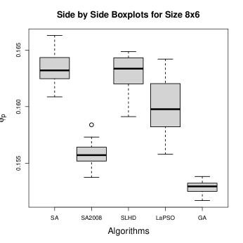
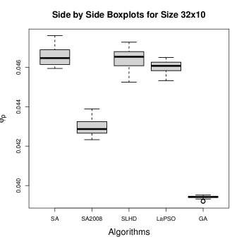
Figure 1: Boxplots for Different Algorithms with Different Sizes based on $\phi_{p}$.

We further display the boxplots of the $\phi_{p}$ values of designs with various run sizes $n$ and factor sizes $k$ for each algorithm. For the case of $n=6$ and $k=4$ (top left panel in Figure 1), the SA2008 is less stable and the LaPSO gives the smallest $\phi_{p}$. When $n\geq 8$ (the other three panels), the variation of LaPSO increases and the GA outperforms the others. When the design sizes become larger, the GA tends to give the smallest $\phi_{p}$ values and is also the most stable algorithm.

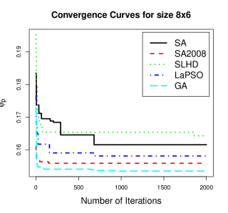
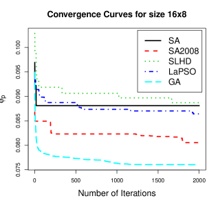
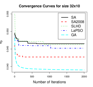
Figure 2: Convergence Curves for Different Algorithms with Different Sizes.

We illustrate the convergence of each algorithm with different $n$ and $k$ in Figure 2. For the case of $n=6$ and $k=4$ (top left panel in Figure 2), the LaPSO gives the smallest $\phi_{p}$ around the $450^{th}$ iteration, while the rest algorithms converge and stop much earlier. This supports the earlier finding that the LaPSO has good performances given enough computational resources for small designs. When $n\geq 8$ (the rest three panels), the GA converges faster than all others with good performances, and the SA2008 is the second best. Note that the GA exchanges columns for generating new candidate designs, while other methods exchange elements. Element-wise operations work well when $n$ and $k$ are relatively small. But, when the design sizes become large, the numbers of elements increase exponentially and the strategy of exchanging elements may become less efficient. The uniqueness of the GA is that the algorithm exchanges the entire columns and thus the computation won’t grow that much for large run sizes.

5.2 Results on Maximum Projection LHDs

Joseph et al. (2015) adopted a simulated annealing algorithm for identifying MaxPro LHDs, which can be implemented by the R package MaxPro (Ba and Joseph, 2018). In this part, we further consider using the LaPSO and GA algorithms to find MaxPro LHDs via minimizing the objective function $\psi$ defined in Equation (2). For each design size, we run every algorithm 20 times and display the best results (i.e. the minimum $\psi$ values) along with the average CPU time in Tables 6, 7 and 8. We show that our proposed methods are more efficient than the R package MaxPro (denoted as “MaxPro” in the tables).

Table 6: Minimum $\psi$ and average CPU time (in seconds) with run size between $2^{2}$ and $2^{3}-1$.

	$k$	2	3	4
$n$		Min(CPU)	Min(CPU)	Min(CPU)
4	MaxPro	0.4513(0)	0.4705(0)	0.4454(0)
	LaPSO	0.4513(13)	0.4705(15)	0.4454(18)
	GA	0.4513(8)	0.4705(8)	0.4454(9)
5	MaxPro	0.3771(0)	0.3561(0)	0.3382(0)
	LaPSO	0.3771(14)	0.3561(17)	0.3382(19)
	GA	0.3771(8)	0.3561(9)	0.3382(9)
6	MaxPro	0.3154(0)	0.2633(0)	0.2746(0)
	LaPSO	0.3154(8)	0.2633(10)	0.2551(12)
	GA	0.3154(5)	0.2633(5)	0.2551(6)
7	MaxPro	0.2511(0)	0.2388(0)	0.2301(0)
	LaPSO	0.2511(9)	0.2254(12)	0.2160(14)
	GA	0.2511(5)	0.2184(5)	0.2113(6)

In Table 6, when the design sizes are small, e.g. $k=2$ with $n\leq 7$, $k=3$ with $n\leq 6$ and $k=4$ with $n\leq 5$, all the three algorithms give the same minimum $\psi$ values, and the MaxPro has the lowest CPU time. For larger design sizes, we can see that the GA will generally lead to the best results, and the LaPSO also performs better than the MaxPro method. In Tables 7 and 8, we show more results for larger run sizes (between $2^{3}$ and $2^{5}$). It is seen that for relatively large design, the GA finds the best designs with smallest $\psi$ values, while the MaxPro requires the lowest CPU time. The LaPSO generally outperforms the MaxPro but requires the highest CPU time among the three.

Table 7: Minimum $\psi$ and average CPU time (in seconds) with run size between $2^{3}$ and $2^{4}-1$.

	$k$	2	3	4	5	6
$n$		Min(CPU)	Min(CPU)	Min(CPU)	Min(CPU)	Min(CPU)
8	MaxPro	0.2240(0)	0.2031(0)	0.1971(0)	0.1982(0)	0.1967(0)
	LaPSO	0.2240(13)	0.1950(17)	0.1861(21)	0.1846(24)	0.1782(28)
	GA	0.2240(6)	0.1737(7)	0.1763(7)	0.1684(8)	0.1660(9)
10	MaxPro	0.1804(0)	0.1674(0)	0.1543(0)	0.1591(0)	0.1548(0)
	LaPSO	0.1769(14)	0.1507(17)	0.1473(21)	0.1415(24)	0.1429(27)
	GA	0.1685(6)	0.1412(6)	0.1306(7)	0.1241(8)	0.1195(9)
12	MaxPro	0.1463(0)	0.1378(0)	0.1276(0)	0.1260(0)	0.1270(0)
	LaPSO	0.1474(18)	0.1259(23)	0.1183(27)	0.1171(32)	0.1134(36)
	GA	0.1330(6)	0.1120(7)	0.1003(8)	0.0969(9)	0.0925(10)
14	MaxPro	0.1270(0)	0.1194(0)	0.1083(0)	0.1041(0)	0.1070(0)
	LaPSO	0.1204(26)	0.1040(32)	0.1030(39)	0.0977(45)	0.0952(52)
	GA	0.1145(8)	0.0914(9)	0.0819(11)	0.0776(12)	0.0751(13)

Table 8: Minimum $\psi$ and average CPU time (in seconds) with run size between $2^{4}$ and $2^{5}$.

	$k$	2	3	4	5	6	7	8
$n$		Min(CPU)	Min(CPU)	Min(CPU)	Min(CPU)	Min(CPU)	Min(CPU)	Min(CPU)
16	MaxPro	0.1072(0)	0.1020(0)	0.0938(0)	0.0938(0)	0.0904(0)	0.0873(0)	0.0855(0)
	LaPSO	0.1052(24)	0.0928(29)	0.0898(38)	0.0828(43)	0.0813(49)	0.0783(55)	0.0798(61)
	GA	0.0975(7)	0.0770(8)	0.0689(10)	0.0640(11)	0.0617(12)	0.0593(13)	0.0579(14)
20	MaxPro	0.0880(0)	0.0817(0)	0.0722(0)	0.0710(0)	0.0679(0)	0.0665(0)	0.0643(0)
	LaPSO	0.0865(27)	0.0730(61)	0.0675(74)	0.0616(86)	0.0631(96)	0.0610(113)	0.0591(124)
	GA	0.0748(7)	0.0579(15)	0.0510(17)	0.0476(20)	0.0450(22)	0.0426(25)	0.0420(27)
24	MaxPro	0.0764(0)	0.0672(0)	0.0605(0)	0.0587(0)	0.0547(0)	0.0528(0)	0.0512(0)
	LaPSO	0.0693(57)	0.0589(78)	0.0528(93)	0.0542(109)	0.0500(124)	0.0482(140)	0.0468(156)
	GA	0.0600(15)	0.0454(19)	0.0393(22)	0.0358(25)	0.0346(28)	0.0331(31)	0.0320(34)
28	MaxPro	0.0636(0)	0.0544(0)	0.0518(0)	0.0485(0)	0.0478(0)	0.0435(0)	0.0426(0)
	LaPSO	0.0610(66)	0.0525(85)	0.0477(102)	0.0451(134)	0.0422(159)	0.0405(178)	0.0398(192)
	GA	0.0501(16)	0.0367(19)	0.0320(22)	0.0292(27)	0.0272(31)	0.0263(34)	0.0256(37)
32	MaxPro	0.0560(0)	0.0454(0)	0.0439(0)	0.0413(0)	0.0394(0)	0.0373(0)	0.0342(0)
	LaPSO	0.0514(98)	0.0449(128)	0.0392(153)	0.0377(179)	0.0355(205)	0.0346(230)	0.0332(255)
	GA	0.0425(24)	0.0307(30)	0.0263(35)	0.0240(40)	0.0226(45)	0.0217(50)	0.0209(55)

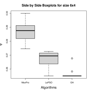
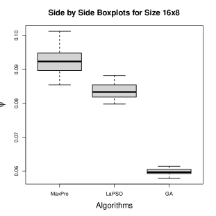
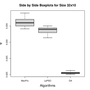
Figure 3: Boxplots for Different Algorithms with Different Sizes based on $\psi$.

Figure 3 illustrates the boxplots of $\psi$ values for each algorithm with different design sizes. From the top left panel in Figure 3 ($k=4$ and $n=6$), it is seen that the MaxPro method is less stable whose boxplot is more stretched, and the GA identifies the best design. When $n\geq 8$ (the other three panels), the GA clearly outperforms other methods, which gives the smallest $\psi$ values and is the most stable. Generally speaking, the proposed GA is recommended for constructing Maxpro LHDs with moderate and large sizes. The CPU time for the GA approach is often reasonable, and it can be further reduced if smaller parameters on the population size and the number of iterations are used. Yet, the MaxPro is the fastest in terms of the CPU time.

5.3 Results on Orthogonal and Nearly Orthogonal LHDs

In this part, we aim to identify orthogonal LHDs (OLHDs) and nearly orthogonal LHDs (NOLHDs) via minimizing the ave$(|q|)$ and max$|q|$ criteria defined in Equation (3). In Tables 9$-$ 11, we show results for some designs with run sizes under $2^{8}$. In these tables, “CM” represents whether there is an available algebraic construction method for the given design size. If “CM” is “Yes”, we should follow the algebraic method to get the corresponding OLHD; otherwise, search algorithms are needed. Please refer to Table 1 in Section 4.2 for the name of the method when “CM” is “Yes”.

Table 9: Minimum ave$(|q|)$, max$|q|$, and average CPU time (in seconds) with run size below $2^{4}$.

$n\times k$	Criteria	SA	SA2008	SLHD	LaPSO	GA	CM
$6\times 4$	ave$(|q|)$	0.0476	0.0286	0.0476	0.0571	0.0286
	max$|q|$	0.0857	0.0286	0.0857	0.0857	0.0286	No
	CPU	15	31	21	33	10
$7\times 4$	ave$(|q|)$	0.0298	0.0060	0.0179	0.0357	0.0119
	max$|q|$	0.0714	0.0357	0.0714	0.0714	0.0357	No
	CPU	15	34	21	34	10
$8\times 4$	ave$(|q|)$	0.0357	0.0000	0.0278	0.0261	0.0119
	max$|q|$	0.0714	0.0000	0.0476	0.0476	0.0238	Yes
	CPU	15	36	21	36	10
$9\times 4$	ave$(|q|)$	0.0111	0.0000	0.0250	0.0222	0.0056
	max$|q|$	0.0500	0.0000	0.0500	0.0333	0.0167	Yes
	CPU	17	44	25	42	12
$10\times 4$	ave$(|q|)$	0.0202	0.0061	0.0222	0.0242	0.0061
	max$|q|$	0.0545	0.0061	0.0424	0.0464	0.0061	No
	CPU	15	42	23	37	11
$10\times 6$	ave$(|q|)$	0.0885	0.0166	0.0990	0.0958	0.0174
	max$|q|$	0.1636	0.0303	0.2242	0.1879	0.0424	No
	CPU	35	77	49	78	21
$12\times 6$	ave$(|q|)$	0.0932	0.0163	0.0839	0.0667	0.0126
	max$|q|$	0.2168	0.0350	0.1608	0.1329	0.0210	No
	CPU	36	86	51	83	21
$14\times 6$	ave$(|q|)$	0.0590	0.0104	0.0708	0.0725	0.0107
	max$|q|$	0.1692	0.0198	0.1516	0.1341	0.0198	No
	CPU	36	96	53	83	21

In Table 9, algebraic constructions exist for two cases ($8\times 4$ and $9\times 4$), and the SA2008 algorithm also identifies these two OLHDs, where both the ave$(|q|)$ and max$|q|$ are $0$. For the rest of the cases, the SA2008 is capable of identifying NOLHDs whose ave$(|q|)$ and max$|q|$ are very small. Generally speaking, the SA2008 outperforms all other search algorithms except for the case of $12\times 6$ where the GA performs better. In Table 10, we further compare the SA2008 and the GA for some larger run sizes. Note that the SA, SLHD and LaPSO methods perform worse than the SA2008 and the GA, and thus we do not include them for conciseness. When $n\geq 16$ and $k\geq 6$, it is seen that the GA provides the best results whose ave$(|q|)$ and max$|q|$ are very small (smaller than $0.03$). Its CPU time is also much lower than that from the SA2008. In Table 11, we further show some cases with run sizes between $2^{5}$ and $2^{8}$. It is seen that there are very few cases where algebraic methods are available, and search algorithms are needed for most cases. From Table 11, we can see that the GA will give designs with max$|q|$ less than $0.03$ for all cases using reasonable CPU time. Overall speaking, the SA2008 has the best performance when $n<16$, and the GA should be used for $n\geq 16$.

Table 10: Minimum ave$(|q|)$, max$|q|$, and average CPU time (in seconds) with run size between $2^{4}$ and $2^{5}-1$.

$n\times k$	Criteria	SA2008	GA	CM		$n\times k$	Criteria	SA2008	GA	CM
$16\times 6$	ave$(|q|)$	0.0110	0.0078			$18\times 8$	ave$(|q|)$	0.0244	0.0148
	max$|q|$	0.0235	0.0147	No			max$|q|$	0.0526	0.0258	No
	CPU	158	32				CPU	182	39
$17\times 6$	ave$(|q|)$	0.0119	0.0077			$22\times 8$	ave$(|q|)$	0.0194	0.0161
	max$|q|$	0.0196	0.0147	Yes			max$|q|$	0.0491	0.0288	No
	CPU	117	22				CPU	222	40
$18\times 6$	ave$(|q|)$	0.0093	0.0058			$28\times 8$	ave$(|q|)$	0.0164	0.0087
	max$|q|$	0.0196	0.0114	No			max$|q|$	0.0427	0.0148	No
	CPU	117	22				CPU	288	40
$17\times 8$	ave$(|q|)$	0.0235	0.0136			$30\times 8$	ave$(|q|)$	0.0160	0.0064
	max$|q|$	0.0637	0.0294	Yes			max$|q|$	0.0420	0.0118	No
	CPU	177	39				CPU	312	40

Table 11: Minimum ave$(|q|)$, max$|q|$, and average CPU time (in minutes) with run size between $2^{5}$ and $2^{8}$.

$n\times k$	Criteria	GA	CM		$n\times k$	Criteria	GA	CM
$33\times 8$	ave$(|q|)$	0.0051			$68\times 10$	ave$(|q|)$	0.0055
	max$|q|$	0.0097	Yes			max$|q|$	0.0092	No
	CPU	1.0				CPU	1.7
$34\times 8$	ave$(|q|)$	0.0047			$96\times 12$	ave$(|q|)$	0.0082
	max$|q|$	0.009	No			max$|q|$	0.0155	No
	CPU	1.0				CPU	3.0
$48\times 10$	ave$(|q|)$	0.0084			$128\times 14$	ave$(|q|)$	0.0125
	max$|q|$	0.0158	No			max$|q|$	0.0219	No
	CPU	1.6				CPU	2.3
$64\times 10$	ave$(|q|)$	0.0066			$192\times 14$	ave$(|q|)$	0.0087
	max$|q|$	0.0122	No			max$|q|$	0.0162	No
	CPU	2.2				CPU	4.9
$65\times 10$	ave$(|q|)$	0.0045			$256\times 16$	ave$(|q|)$	0.0155
	max$|q|$	0.0087	Yes			max$|q|$	0.0278	No
	CPU	1.7				CPU	5.9

Finally, we conducted simulations according to the rule of thumb ($n=10k$) for computer experiments in the literature Chapman et al. (1994); Jones et al. (1998); Loeppky et al. (2009) under various optimality criteria discussed above. The results are presented in Table 12, where the best designs along with average CPU time (in minutes) are presented. For the Maximin distance LHDs, results are based on the $L_{2}$ distance. In Table 12, the GA outperforms the other algorithms in terms of $\phi_{p}$ values. Except for the construction method FastMm, the GA requires the lowest CPU time. The SA2008 has the second smallest $\phi_{p}$ values but the highest CPU time. For $\psi$ values, the GA provides the best results and the MaxPro has the lowest CPU time. These conclusions are consistent with the discussions above. For the $20\times 2$ design, all the five algorithms successfully identified the OLHDs, where the GA and the SA have the lowest CPU time. For the cases of $k\geq 3$, the GA gives the max$|q|$ values less than $0.0022$ for all cases, and its CPU time are also the lowest. Overall speaking, the GA is recommended for generating designs with the rule of thumb sizes.

Table 12: Results of LHDs with the rule of thumb sizes under different optimality criteria.

	$n\times k$	20 $\times$ 2	30 $\times$ 3	40 $\times$ 4	50 $\times$ 5	60 $\times$ 6	70 $\times$ 7	80 $\times$ 8
Criteria		Min(CPU)	Min(CPU)	Min(CPU)	Min(CPU)	Min(CPU)	Min(CPU)	Min(CPU)
$\phi_{p}$	SA	0.3364(1.4)	0.1636(3.7)	0.0990(12.1)	0.0676(22.1)	0.0498(36.2)	0.0376(56.5)	0.0299(49.6)
	SA2008	0.2960(2.4)	0.1449(6.1)	0.0882(19.3)	0.0589(34.7)	0.0434(55.6)	0.0331(85.1)	0.0262(76.0)
	SLHD	0.3269(2.0)	0.1662(5.3)	0.0990(17.2)	0.0671(31.6)	0.0488(51.1)	0.0376(79.7)	0.0296(69.9)
	LaPSO	0.3370(3.0)	0.1603(7.7)	0.0975(24.7)	0.0668(45.4)	0.0488(73.6)	0.0362(100.0)	0.0291(99.8)
	GA	0.2802(0.8)	0.1262(1.9)	0.0738(6.1)	0.0502(11.2)	0.0370(18.1)	0.0288(28.4)	0.0233(25.0)
	FastMm	0.4905(0)	0.1616(0)	0.0941(0)	0.0632(0)	0.0458(0)	0.0341(0)	0.0270(0)
$\psi$	MaxPro	0.0880(0)	0.0522(0)	0.0343(0)	0.0232(0)	0.0171(0)	0.0129(0)	0.0100(0)
	LaPSO	0.0865(0.4)	0.0483(1.1)	0.0317(2.1)	0.0227(3.7)	0.0165(9.3)	0.0124(14.0)	0.0102(19.9)
	GA	0.0748(0.1)	0.0335(0.2)	0.0193(0.4)	0.0128(0.8)	0.0092(2.0)	0.0070(3.1)	0.0055(4.4)
ave$(|q|)$	SA	0(0.1)	0.0014(0.3)	0.0137(0.5)	0.0262(0.8)	0.0305(1.2)	0.0422(1.7)	0.0510(2.2)
	SA2008	0(1.7)	0.0002(4.2)	0.0008(7.6)	0.0023(12.8)	0.0045(20.4)	0.0050(30.4)	0.0092(41.5)
	SLHD	0(0.4)	0.0014(0.9)	0.0079(1.7)	0.0138(2.9)	0.0292(4.6)	0.0425(7.0)	0.0480(9.1)
	LaPSO	0(0.4)	0.0013(1.0)	0.0049(1.7)	0.0161(2.8)	0.0270(4.2)	0.0380(5.8)	0.0415(7.7)
	GA	0(0.1)	0.0002(0.2)	0.0003(0.3)	0.0004(0.5)	0.0005(0.7)	0.0007(0.9)	0.0011(1.3)
max$|q|$	SA	0(0.1)	0.0020(0.3)	0.0227(0.5)	0.0457(0.8)	0.0624(1.2)	0.0940(1.7)	0.1058(2.2)
	SA2008	0(1.7)	0.0002(4.2)	0.0019(7.6)	0.0053(12.8)	0.0129(20.4)	0.0117(30.4)	0.0246(41.5)
	SLHD	0(0.4)	0.0016(0.9)	0.0205(1.7)	0.0385(2.9)	0.0598(4.6)	0.0854(7.0)	0.0989(9.1)
	LaPSO	0(0.4)	0.0020(1.0)	0.0120(1.7)	0.0341(2.8)	0.0554(4.2)	0.0878(5.8)	0.0853(7.7)
	GA	0(0.1)	0.0002(0.2)	0.0006(0.3)	0.0007(0.5)	0.0009(0.7)	0.0015(0.9)	0.0022(1.3)

6 Conclusion

In this paper, we discussed the constructions of three types of efficient LHDs, namely, the maximin distance LHDs, the maximum projection LHDs and the (nearly) orthogonal LHDs. We reviewed, summarized and compared some currently popular search algorithms (including the SA by Morris and Mitchell (1995), SA2008 by Joseph and Hung (2008), SLHD by Ba et al. (2015), LaPSO by Chen et al. (2013) and GA by Liefvendahl and Stocki (2006)) and many algebraic constructions (Wang et al., 2018; Ye, 1998; Cioppa and Lucas, 2007; Sun et al., 2010; Tang, 1993; Lin et al., 2009; Butler, 2001). We developed efficient implementations of these methods and integrated them into the R package LHD. Algebraic constructions are generally preferred, especially for large designs. Yet, they are only available for certain design sizes. Search algorithms are required to generate efficient LHDs with flexible sizes.

From the numerical studies in Section 5, we provided some recommendations on the search algorithms for practitioners. Generally speaking, the GA is the most desirable approach to generate efficient LHDs, which provides a good balance between the performance and the CPU time. It outperforms other search algorithms for moderate and large design sizes. The SA2008 performs very well for generating maximin distance LHDs and OLHDs (NOLHDs), but often requires much longer CPU time, which is more suitable for small design sizes. For generating MaxPro LHDs, the R package MaxPro (Ba and Joseph, 2018) is the fastest, but the resulting designs are often worse than the ones found by the GA implemented by our R package LHD.

The search algorithms discussed in this paper can also generate other types of efficient experimental designs. An interesting future research is to expand the scope of this paper, and further consider various design types, including the fractional factorial designs (Dean et al., 2017), supersaturate designs (Lin, 1993) and order-of-addition designs (Peng et al., 2019). We aim to compare different algorithms under different design optimality criteria, and provide recommendations for experimenters who need to use efficient designs but have limited knowledge on design theories. We plan to develop a comprehensive R package implemented with efficient coding for practitioners.

7 Appendix

Here we demonstrate how to use the functions in our developed R package LHD (Wang et al., 2020) to implement the algorithms and the algebraic constructions discussed in the paper. Examples are provided to illustrate how to set input arguments and tuning parameters.

7.1 Basic Functions

There are six basic functions in the LHD package and they are listed in Table A1. Functions phi_p, MaxProCriterion, AvgAbsCor, and MaxAbsCor are the optimality criteria presented in Section 2 of the paper. The following examples demonstrate how to use them.

⬇

> X=rLHD(n=5,k=3);X #This generates a 5 by 3 random LHD, denoted as X

[,1] [,2] [,3]

[1,] 2 1 4

[2,] 4 3 3

[3,] 3 2 2

[4,] 1 4 5

[5,] 5 5 1 \par#To evaluate the design matrix X in terms of different optimality criteria:

> phi_p(X) #the maximin distance criterion.

[1] 0.3336608

> MaxProCriterion(X) #the maximum projection Criterion.

[1] 0.5375482

> AvgAbsCor(X) #the average absolute correlation.

[1] 0.5333333

> MaxAbsCor(X) #the maximum absolute correlation.

[1] 0.9

Note that the default settings for phi_p is $p=15$ and $q=1$ (the Manhattan distance) and user can change the settings.

⬇

> phi_p(X,p=10,q=2)

[1] 0.5797347

\par\par> WT(X) #Apply the Williams transformation on X

[,1] [,2] [,3]

[1,] 3 1 4

[2,] 4 5 5

[3,] 5 3 3

[4,] 1 4 2

[5,] 2 2 1

\par> phi_p(WT(X)) #The phi_p value of transformed X is smaller than before

[1] 0.2517886

\par

Table A1: Basic functions in the LHD package

Function	Description
rLHD	Returns a random LHD matrix with user-defined dimension.
phi_p	Implements the $\phi_{p}$ criterion (Morris and Mitchell, 1995; Jin et al., 2005) of a matrix.
MaxProCriterion	Implements the maximum projection criterion (Joseph et al., 2015) of a matrix.
AvgAbsCor	Returns the average absolute correlation (Georgiou, 2009) of a matrix.
MaxAbsCor	Returns the maximum absolute correlation (Georgiou, 2009) of a matrix.
WT	Implements the Williams transformation (Williams, 1949) of a matrix.

7.2 Search Algorithm Functions

Six algorithm functions are listed in Table A2, where functions SA, OASA, SA2008 and SLHD are simulated annealing (SA) based algorithms. All the six algorithms were demonstrated in Section 3, and they can be used to identify different types of efficient LHDs. For users who seek fast solutions, simply indicate the design sizes and/or the factor sizes, and leave the rest input arguments with the default settings. See the following examples.

Table A2: Search algorithm functions in the LHD package

Function	Description
SA	Returns an LHD via the simulated annealing algorithm (Morris and Mitchell, 1995).
OASA	Returns an LHD via the orthogonal-array-based simulated annealing algorithm
	by Leary et al. (2003), where an OA of the required design size must exist.
SA2008	Returns an LHD via the simulated annealing algorithm with the multi-objective
	optimization approach by Joseph and Hung (2008).
SLHD	Returns an LHD via the improved two-stage algorithm by Ba et al. (2015).
LaPSO	Returns an LHD via the particle swarm optimization by Chen et al. (2013).
GA	Returns an LHD via the genetic algorithm by Liefvendahl and Stocki (2006).

⬇

#Generate a 5 by 3 maximin distance LHD by the SA function.

> try.SA=SA(n=5,k=3); try.SA

[,1] [,2] [,3]

[1,] 2 2 1

[2,] 5 3 2

[3,] 4 5 5

[4,] 3 1 4

[5,] 1 4 3

> phi_p(try.SA) #\phi_p is smaller than that of a random LHD (0.3336608).

[1] 0.2169567

\par#Generates a 5 by 3 maximin distance LHD by the SA2008, SLHD, LaPSO

# and GA functions.

> try.SA2008=SA2008(n=5,k=3)

> try.SLHD=SLHD(n=5,k=3)

> try.LaPSO=LaPSO(n=5,k=3)

> try.GA=GA(n=5,k=3)

\par#create an OA(9,2,3,2).

> OA=matrix(c(rep(1:3,each=3),rep(1:3,times=3)),

+ ncol=2,nrow=9,byrow = FALSE)

#OASA(OA) generates a maximin distance LHD with the same size of the input OA

#by the orthogonal-array-based simulated annealing algorithm.

> try.OASA=OASA(OA)

>OA; try.OASA

[,1] [,2] [,1] [,2]

[1,] 1 1 [1,] 1 2

[2,] 1 2 [2,] 2 6

[3,] 1 3 [3,] 3 9

[4,] 2 1 [4,] 4 3

[5,] 2 2 [5,] 6 5

[6,] 2 3 [6,] 5 7

[7,] 3 1 [7,] 7 1

[8,] 3 2 [8,] 9 4

[9,] 3 3; [9,] 8 8

\par

Note that the default optimality criterion embedded in the above algorithm functions is $\phi_{p}$, and thus they lead to the maximin distance LHDs. When other optimality criteria are used, users can change the input argument OC (including options “phi_p”, “MaxProCriterion”, “MaxAbsCor” and “MaxProCriterion”). The following examples illustrate some details on setting the input arguments to customize the functions.

⬇

#Design try.SA is a 5 by 3 maximin distance LHD generated by the SA with

#30 iterations. The temperature starts at 10 and decreases 10#The minimium temperature allowed is 1 and the maximum perturbations that

#the algorithm will try without improvements is 5. The optimality criterion

#used is \phi_p with p=15 and q=1, and the maximum CPU time is 5 minutes.

> try.SA=SA(n=5,k=3,N=30,T0=10,rate=0.1,Tmin=1,Imax=5,OC=”phi_p”,

+ p=15,q=1,maxtime=5); try.SA

[,1] [,2] [,3]

[1,] 1 3 4

[2,] 2 5 2

[3,] 5 4 3

[4,] 4 1 5

[5,] 3 2 1

> phi_p(try.SA)

[1] 0.2169567

\par#try.SA2008 below is a 5 by 3 maximin distance LHD generated by SA with

#multi-objective optimization approach.

> try.SA2008=SA2008(n=5,k=3,N=30,T0=10,rate=0.1,Tmin=1,Imax=5,

+ OC=”phi_p”,p=15,q=1,maxtime=5)

\par#try.SLHD below is a 5 by 3 maximin distance LHD generated by improved

#two-stage algorithm with only 1 slice (t=1), and the second stage of

#the algorithm would be implemented.

> try.SLHD=SLHD(n=5,k=3,t=1,N=30,T0=10,rate=0.1,Tmin=1,Imax=5,

+ OC=”phi_p”,p=15,q=1,stage2=TRUE,maxtime=5)

\par#try.OASA below is a 9 by 2 maximin distance LHD generated by the

#orthogonal-array-based simulated annealing algorithm with the input

#OA defined previously and the rest arguments are interpreted the

#same as try.SA above.

> try.OASA=OASA(OA,N=30,T0=10,rate=0.1,Tmin=1,Imax=5,OC=”phi_p”,p=15,

+ q=1,maxtime=5)

\par#try.LaPSO below is a 5 by 3 maximum projection LHD generated by the

#particle swarm optimization algorithm with 20 particles and 30

#iterations. Zero (or two) elements in any column of the current particle

#should be the same as the corresponding personal best (or global best).

#The probability of exchanging two randomly selected elements is 0.5,

#and the maximum CPU time is 5 minutes.

> try.LaPSO=LaPSO(n=5,k=3,m=20,N=30,SameNumP=0,SameNumG=2,p0=0.5,

+ OC=”MaxProCriterion”,maxtime=5); try.LaPSO

[,1] [,2] [,3]

[1,] 4 5 4

[2,] 3 1 3

[3,] 5 2 1

[4,] 2 3 5

[5,] 1 4 2

#Compare to the value of 0.5375482 from the above random LHD

> MaxProCriterion(try.LaPSO)

[1] 0.3561056

\par#try.GA below is a 5 by 3 OLHD generated by the genetic algorithm

#with the population size 20, number of iterations 30, mutation

#probability 0.5 and the maximum CPU time 5 minutes.

> try.GA=GA(n=5,k=3,m=20,N=30,pmut=0.5,OC=”MaxAbsCor”,maxtime=5)

Next, we discuss some implementation details. In the SA based algorithms (SA, SA2008, SLHD and OASA), the number of iterations N is recommended to be no greater than 500 according to the convergence curves in Figure 2 of Section 5. Input rate determines the percent of the current temperature decreased (e.g. $0.1$ means a decrease of $10\%$ each time). A high rate would make the temperature decline quickly, which leads to a fast stop of the algorithm. It is recommended to be from $0.1$ to $0.15$. Imax indicates the maximum perturbations that the algorithm will try without improvements before the temperature reduces, and it is recommended to be no greater than 5 for computation consideration. OC chooses the optimality criterion and uses the "phi_p" by default, which identifies the maximin distance LHDs. OC could be changed to "MaxProCriterion", "AvgAbsCor" and "MaxAbsCor". The function SLHD has two additional input arguments, which are t and stage2. Here t is the number of slices in the design. SLHD can be used as a modified SA algorithm when t is 1. stage2 is a logical argument (either TRUE or FALSE) which determines if the second stage of the algorithm would be implemented, and it is recommended to set as FALSE when computational budgets are limited.

For the function LaPSO, the input m is the number of particles. There are three tuning parameters: SameNumP, SameNumG and p0. SameNumP and SameNumG denote how many exchanges would be performed to reduce the Hamming distance towards the personal best and the global best. p0 denote the probability of a random swap for two elements in the current column of the current particle. In Chen et al. (2013), they provided the following suggestions: SameNumP is approximately $n/2$ when SameNumG is $0$, SameNumG is approximately $n/4$ when SameNumP is $0$, and p0 should be between $1/(k-1)$ and $2/(k-1)$. For function GA, input m is the population size. The only tuning parameter: the mutation probability pmut, is recommended to be $1/(k-1)$. All algorithm functions will show a progress bar when running. After an algorithm completes, information of average CPU time per iteration and the number of iterations completed would be presented. Users can set the maximum CPU time limit for each algorithm via the argument maxtime. Our algorithms support both the $L_{1}$ and $L_{2}$ distances.

7.3 Algebraic Construction Functions

The developed LHD package supports seven algebraic construction methods, which are listed in Table A3. FastMmLHD and OA2LHD are for maximin distance LHDs. OLHD.Y1998, OLHD.C2007, OLHD.S2010, OLHD.L2009, and OLHD.B2001 are for orthogonal LHDs. All the seven methods were discussed in Section 4. The following examples illustrate how to use them.

Table A3: Algebraic construction methods in the LHD package

Function	Description
FastMmLHD	Returns a maximin distance LHD matrix by Wang et al. (2018).
OLHD.Y1998	Returns a $2^{m}+1$ by $2m-2$ orthogonal LHD matrix generated by
	Ye (1998) where $m$ is an integer and $m\geq 2$.
OLHD.C2007	Returns a $2^{m}+1$ by $m+{m-1\choose 2}$ orthogonal LHD matrix by
	Cioppa and Lucas (2007) where $m$ is an integer and $m\geq 2$.
OLHD.S2010	Returns a $r2^{c+1}+1$ or $r2^{c+1}$ by $2^{c}$ orthogonal LHD matrix by
	Sun et al. (2010) where $r$ and $c$ are positive integers.
OA2LHD	Expands an orthogonal array to an LHD by Tang (1993).
OLHD.L2009	Couples an $n$ by $p$ orthogonal LHD with a $n^{2}$ by $2f$ strength $2$ and
	level $n$ orthogonal array to generate a $n^{2}$ by $2fp$ orthogonal LHD
	by Lin et al. (2009).
OLHD.B2001	Returns an orthogonal LHD by Butler (2001) with the run size
	being odd primes.

⬇

\par#FastMmLHD(8,8) generates an optimal 8 by 8 maximin L_1 distance LHD.

>try.FastMm=FastMmLHD(n=8,k=8); try.FastMm

\par[,1] [,2] [,3] [,4] [,5] [,6] [,7] [,8]

[1,] 0 1 2 3 4 5 6 7

[2,] 1 3 5 7 6 4 2 0

[3,] 2 5 7 4 1 0 3 6

[4,] 3 7 4 0 2 6 5 1

[5,] 4 6 1 2 7 3 0 5

[6,] 5 4 0 6 3 1 7 2

[7,] 6 2 3 5 0 7 1 4

[8,] 7 0 6 1 5 2 4 3

\par#OA2LHD(OA) expands an input OA to an LHD of the same run size.

>try.OA2LHD=OA2LHD(OA)

>OA; try.OA2LHD

[,1] [,2] [,1] [,2]

[1,] 1 1 [1,] 1 2

[2,] 1 2 [2,] 2 4

[3,] 1 3 [3,] 3 9

[4,] 2 1 [4,] 4 3

[5,] 2 2 [5,] 5 5

[6,] 2 3 [6,] 6 7

[7,] 3 1 [7,] 9 1

[8,] 3 2 [8,] 8 6

[9,] 3 3; [9,] 7 8

⬇

#OLHD.Y1998(m=3) generates a 9 by 4 orthogonal LHD.

#Note that 2^m+1=9 and 2*m-2=4.

> try.Y1998=OLHD.Y1998(m=3);try.Y1998

[,1] [,2] [,3] [,4]

[1,] 4 -3 -2 1

[2,] 3 4 -1 -2

[3,] 1 -2 3 -4

[4,] 2 1 4 3

[5,] 0 0 0 0

[6,] -4 3 2 -1

[7,] -3 -4 1 2

[8,] -1 2 -3 4

[9,] -2 -1 -4 -3

> MaxAbsCor(try.Y1998) #column-wise correlations are 0.

[1] 0

\par\par#OLHD.C2007(m=4) generates a 17 by 7 orthogonal LHD.

#Note that 2^m+1=17 and $4+{4-1 \choose2}$=7.

> try.C2007=OLHD.C2007(m=4); dim(try.C2007)

[1] 17 7

> MaxAbsCor(try.C2007) #column-wise correlations are 0

[1] 0

\par#OLHD.S2010(C=3,r=3,type=”odd”) generates a 49 by 8 orthogonal LHD.

#Note that 3*2^4+1=49 and 2^3=8.

> dim(OLHD.S2010(C=3,r=3,type=”odd”))

[1] 49 8

> MaxAbsCor(OLHD.S2010(C=3,r=3,type=”odd”)) #column-wise correlations are 0

[1] 0

\par#OLHD.S2010(C=3,r=3,type=”even”) generates a 48 by 8 orthogonal LHD.

#Note that 3*2^4=48 and 2^3=8.

> dim(OLHD.S2010(C=3,r=3,type=”even”))

[1] 48 8

> MaxAbsCor(OLHD.S2010(C=3,r=3,type=”even”)) #column-wise correlations are 0

[1] 0

\par#Create a 5 by 2 OLHD.

OLHD=OLHD.C2007(m=2)

\par#Create an OA(25,6,5,2).

OA=matrix(c(2,2,2,2,2,1,2,1,5,4,3,5,3,2,1,5,4,5,1,5,4,3,2,5,

4,1,3,5,2,3,1,2,3,4,5,2,1,3,5,2,4,3,1,1,1,1,1,1,4,3,2,1,5,5,

5,5,5,5,5,1,4,4,4,4,4,1,3,1,4,2,5,4,3,3,3,3,3,1,3,5,2,4,1,3,

3,4,5,1,2,2,5,4,3,2,1,5,2,3,4,5,1,2,2,5,3,1,4,4,1,4,2,5,3,4,

4,2,5,3,1,4,2,4,1,3,5,3,5,3,1,4,2,4,5,2,4,1,3,3,5,1,2,3,4,2,

4,5,1,2,3,2),ncol=6,nrow=25,byrow=TRUE)

\par#OLHD.L2009(OLHD,OA) generates a 25 by 12 orthogonal LHD.

#Note that n=5 so n^2=25. p=2 and f=3 so 2fp=12.

> dim(OLHD.L2009(OLHD,OA))

[1] 25 12

> MaxAbsCor(OLHD.L2009(OLHD,OA)) #column-wise correlations are 0.

[1] 0

\par#OLHD.B2001(n=11,k=5) generates a 11 by 5 orthogonal LHD.

> dim(OLHD.B2001(n=11,k=5))

[1] 11 5

\par

References

- Ba and Joseph (2018) Ba, S., Joseph, V.R., 2018. MaxPro: Maximum Projection Designs. URL: https://CRAN.R-project.org/package=MaxPro. r package version 4.1-2.
- Ba et al. (2015) Ba, S., Myers, W.R., Brenneman, W.A., 2015. Optimal sliced Latin hypercube designs. Technometrics 57, 479–487.
- Butler (2001) Butler, N.A., 2001. Optimal and orthogonal Latin hypercube designs for computer experiments. Biometrika 88, 847–857.
- Chapman et al. (1994) Chapman, W.L., Welch, W.J., Bowman, K.P., Sacks, J., Walsh, J.E., 1994. Arctic sea ice variability: Model sensitivities and a multidecadal simulation. Journal of Geophysical Research: Oceans 99, 919–935.
- Chen et al. (2015) Chen, R.B., Chang, S.P., Wang, W., Tung, H.C., Wong, W.K., 2015. Minimax optimal designs via particle swarm optimization methods. Statistics and Computing 25, 975–988.
- Chen et al. (2013) Chen, R.B., Hsieh, D.N., Hung, Y., Wang, W., 2013. Optimizing Latin hypercube designs by particle swarm. Statistics and computing 23, 663–676.
- Cioppa and Lucas (2007) Cioppa, T.M., Lucas, T.W., 2007. Efficient nearly orthogonal and space-filling Latin hypercubes. Technometrics 49, 45–55.
- Dean et al. (2017) Dean, A., Voss, D., Draguljić, D., et al., 2017. Design and analysis of experiments. Springer International Publishing.
- Fang et al. (2005) Fang, K.T., Li, R., Sudjianto, A., 2005. Design and modeling for computer experiments. CRC press.
- Fang et al. (2002) Fang, K.T., Ma, C.X., Winker, P., 2002. Centered -discrepancy of random sampling and Latin hypercube design, and construction of uniform designs. Mathematics of Computation 71, 275–296.
- Georgiou (2009) Georgiou, S.D., 2009. Orthogonal Latin hypercube designs from generalized orthogonal designs. Journal of Statistical Planning and Inference 139, 1530–1540.
- Georgiou and Efthimiou (2014) Georgiou, S.D., Efthimiou, I., 2014. Some classes of orthogonal Latin hypercube designs. Statistica Sinica 24, 101–120.
- Goldberg (1989) Goldberg, D.E., 1989. Genetic algorithms in search. Optimization, and MachineLearning .
- Grosso et al. (2009) Grosso, A., Jamali, A., Locatelli, M., 2009. Finding maximin Latin hypercube designs by iterated local search heuristics. European Journal of Operational Research 197, 541–547.
- Hickernell (1998) Hickernell, F., 1998. A generalized discrepancy and quadrature error bound. Mathematics of computation 67, 299–322.
- Holland et al. (1992) Holland, J.H., et al., 1992. Adaptation in natural and artificial systems: an introductory analysis with applications to biology, control, and artificial intelligence. MIT press.
- Jin et al. (2005) Jin, R., Chen, W., Sudjianto, A., 2005. An efficient algorithm for constructing optimal design of computer experiments. Journal of statistical planning and inference 134, 268–287.
- Johnson et al. (1990) Johnson, M.E., Moore, L.M., Ylvisaker, D., 1990. Minimax and maximin distance designs. Journal of statistical planning and inference 26, 131–148.
- Jones et al. (1998) Jones, D.R., Schonlau, M., Welch, W.J., 1998. Efficient global optimization of expensive black-box functions. Journal of Global optimization 13, 455–492.
- Joseph et al. (2015) Joseph, V.R., Gul, E., Ba, S., 2015. Maximum projection designs for computer experiments. Biometrika 102, 371–380.
- Joseph and Hung (2008) Joseph, V.R., Hung, Y., 2008. Orthogonal-maximin Latin hypercube designs. Statistica Sinica , 171–186.
- Kennedy and Eberhart (1995) Kennedy, J., Eberhart, R., 1995. Particle swarm optimization, in: Proceedings of ICNN’95-International Conference on Neural Networks, IEEE. pp. 1942–1948.
- Kirkpatrick et al. (1983) Kirkpatrick, S., Gelatt, C.D., Vecchi, M.P., 1983. Optimization by simulated annealing. science 220, 671–680.
- Leary et al. (2003) Leary, S., Bhaskar, A., Keane, A., 2003. Optimal orthogonal-array-based Latin hypercubes. Journal of Applied Statistics 30, 585–598.