Robust Learning under Strong Noise via SQs

Abstract

This work provides several new insights on the robustness of Kearns’ statistical query framework against challenging label-noise models. First, we build on a recent result by Chen et al. (2020) that showed noise tolerance of distribution-independently evolvable concept classes under Massart noise. Specifically, we extend their characterization to more general noise models, including the Tsybakov model which considerably generalizes the Massart condition by allowing the flipping probability to be arbitrarily close to $\frac{1}{2}$ for a subset of the domain. As a corollary, we employ an evolutionary algorithm by Kanade et al. (2010) to obtain the first polynomial time algorithm with arbitrarily small excess error for learning linear threshold functions over any spherically symmetric distribution in the presence of spherically symmetric Tsybakov noise. Moreover, we posit access to a stronger oracle, in which for every labeled example we additionally obtain its flipping probability. In this model, we show that every SQ learnable class admits an efficient learning algorithm with $\operatorname{OPT}+\epsilon$ misclassification error for a broad class of noise models. This setting substantially generalizes the widely-studied problem of classification under RCN with known noise rate, and corresponds to a non-convex optimization problem even when the noise function – i.e. the flipping probabilities of all points – is known in advance.

1 Introduction

Label noise is a critical impediment in machine learning as it may dramatically reduce the accuracy of the classifier and augment the computational and sample requirements of the learning algorithm. Naturally, designing efficient and noise tolerant paradigms has been a central endeavor from the inception of machine learning with Rosenblatt’s celebrated perceptron algorithm (Rosenblatt (1958)). Indeed, a vast body of work has been devoted to tackling different types of label noise. As it turns out, the guarantees we can hope for crucially depend on the underlying noise model. In the agnostic model (Haussler (1992); Kearns et al. (1992)) – where an adversary is allowed to corrupt some fraction of the labels arbitrarily – even weak learning is known to be NP-hard (Feldman et al. (2006); Guruswami and Raghavendra (2006); Daniely (2016)), while the best results require additional assumptions on the marginal distribution over the instance space, and obtain much weaker multiplicative approximations (Daniely (2015); Awasthi et al. (2014)). On the other hand, in the random classification noise (henceforth RCN) of Angluin and Laird (1987) – where the label of each example is flipped independently with some fixed probability $\gamma<\frac{1}{2}$ – strong positive results have been established, commencing from Bylander (1994) and Blum et al. (1996). Typical approaches to learn in the presence of noise include empirical risk minimization (ERM) (Manwani and Sastry (2013)) with a smooth and convex surrogate of the $0-1$ loss (Bartlett et al. (2006)), boosting techniques (Friedman et al. (2000); Freund (1999)), variants of the perceptron algorithm (Li and Long (1999); Khardon and Wachman (2007)), and SVMs (Ganapathiraju and Picone (2000); Lin and Wang (2004)).

Moreover, a powerful technique for designing noise tolerant algorithms was introduced by Kearns (1998) in the form of the statistical query (SQ) framework, a natural restriction to Valiant’s PAC learning model (Valiant (1984)) in which the learner employs ”large” samples, instead of properties of specific individual examples. Importantly, Kearns demonstrated that any procedure based on statistical queries can be automatically converted to a learning algorithm robust to the RCN model, with rate smaller than the information-theoretic barrier of $\frac{1}{2}$. In fact, virtually all PAC learnable concept classes are also learnable with access to statistical queries; a notable exception is the class of parities that includes all functions equal to an XOR of some subset of Boolean variables (Blum et al. (2003)). As a result, most RCN-tolerant PAC learning algorithms were either derived from the SQ model, or can be easily cast into it. Our work follows this long line of research and strengthens prior results along several lines, extending the robustness of the SQ framework against more challenging noise models.

In the first part of our work we consider the standard noisy oracle model, defined in the following generic form:

Definition 1.1 (Noisy Oracle).

Let $f$ be an unknown target function in a family of Boolean functions $\mathcal{C}$ over $\mathcal{X}\subseteq\mathbb{R}^{d}$, $\mathcal{D}_{\mathbf{x}}$ an arbitrary distribution over $\mathcal{X}$, and $\eta:\mathcal{X}\mapsto\left[0,\frac{1}{2}\right)$ an unknown function. A noisy oracle $\operatorname{EX^{noisy}}_{o}racle(f,\mathcal{D}_{\mathbf{x}},\eta)$ returns a labeled example $(\mathbf{x},y)$, where $\mathbf{x}\sim\mathcal{D}_{\mathbf{x}}$, $y=f(\mathbf{x})$ with probability $1-\eta(\mathbf{x})$ and $y=-f(\mathbf{x})$ with probability $\eta(\mathbf{x})$. We let $\mathcal{D}$ represent the joint distribution on $(\mathbf{x},y)$ generated by the above oracle.

Of course, the known guarantees crucially depend on the assumptions we make on the noise function $\eta$. As we previously discussed, the special case of the RCN model – i.e. $\eta(\mathbf{x})=\gamma<\frac{1}{2}$ – is known to be efficiently addressed due to the symmetry of the underlying noise. A much more realistic and widely-studied condition that has received considerable attention in computational learning theory in recent years (Awasthi et al. (2016); Zhang et al. (2017); Yan and Zhang (2017); Zhang et al. (2020); Awasthi et al. (2015); Diakonikolas et al. (2020b, 2019); Chen et al. (2020)) is the so-called Massart or bounded model (Massart and Nédélec (2006)), where $\eta(\mathbf{x})\leq\gamma$ for some parameter $\gamma\in\left[0,\frac{1}{2}\right)$. In this paper, we are tackling a substantially more general model than the Massart, defined as follows.

Definition 1.2 (Tsybakov noise).

A noise function $\eta$ satisfies the $(\alpha,A,t_{0})$-Tsybakov condition with $\alpha\in(0,1)$, $A>0$, and $t_{0}\in\left(0,\frac{1}{2}\right]$ if

$$\operatorname{\mathbf{Pr}}_{\mathbf{x}\sim\mathcal{D}_{\mathbf{x}}}\left[\eta(\mathbf{x})\geq\frac{1}{2}-t\right]\leq At^{\frac{\alpha}{1-\alpha}},$$ (1)

for all $t\in[0,t_{0}]$.

Thus, the Tsybakov condition allows the flipping probability to be arbitrarily close to $\frac{1}{2}$ for a subset of the domain, and as such, it strictly generalizes the Massart condition. Indeed, for $\alpha\to 1$ it follows that $t^{\frac{\alpha}{1-\alpha}}\to 0$, and hence, the Tsybakov condition yields a $\gamma$-Massart noise with $\gamma=\frac{1}{2}-t_{0}$. This particular noise model was introduced by Mammen and Tsybakov (1999) in a slightly stronger form, and it was subsequently refined by Tsybakov (2004). However, although the information-theoretic aspects of the Tsybakov noise have been well-understood in statistics (Boucheron et al. (2005); Bartlett et al. (2006); Blanchard et al. (2003); Morel et al. (2007); Koltchinskii (2006); Hanneke and Yang (2015)), developing computationally efficient algorithms has remained elusive and a notable open problem in computational learning theory. Importantly, the techniques employed in the Massart model inherently fail and new algorithmic ideas are required. In this context, we build on a recent result of Chen et al. (2020) which showed that Valiant’s notion of evolvability (Valiant (2009)) implies efficient learnability in the presence of Massart noise. Our first contribution is to extend their characterization to a broader class of noise models, and as a corollary, we establish a polynomial time algorithm with arbitrarily small excess error in the presence of spherically symmetric Tsybakov noise.

In the second part of our study we posit a stronger oracle. Specifically, we assume that for every labeled example $(\mathbf{x},y)$ drawn from $\mathcal{D}$ we additionally obtain its corruption rate $\eta(\mathbf{x})$. This model strongly generalizes the widely-studied RCN with known rate, and is motivated in a number of practical applications. Indeed, label-noise typically reflects a measure of confidence or uncertainty of the experts with respect to the given instance (Frénay and Verleysen (2014)), and it is natural to assume that the expert can provide a quantifiable measure of that uncertainty. In some cases multiple experts may be employed in order to determine the label in a subjective task (Dawid and Skene (1979)), and the error rate can be approximated through the disagreement among the experts; typical scenarios include medical applications (Malossini et al. (2006)) and image data analysis (Smyth et al. (1994); Smyth (1996)). Moreover, label noise may be also caused from communication errors (Brodley and Friedl (1999)) and knowing the reliability of the different channels of communication would provide an estimate of the noise rate for every observed labeled example. Finally, stochastic label noise can be intentionally introduced in order to protect the agents’ privacy; in such cases, the noise may be fully specified (van den Hout and van der Heijden (2002)) and the crucial question is how robust is the system to potential leakage of the noise function to adversarial and potentially malicious parties.

Our key contribution in this model is to show that with access to such an oracle, every concept class efficiently learnable with statistical queries admits a polynomial time learning algorithm with arbitrarily small excess error for a broad class of noise models, including Massart and Tsybakov. Our argument extends Kearns’ celebrated simulation of statistical queries in the presence of RCN, and is of particular importance in light of lower bounds against convex surrogates in the presence of Massart noise, applicable even when the noise function is known (Diakonikolas et al. (2019)).

1.1 Related Work

Developing efficient and noise tolerant algorithms via the statistical query framework has been an area of prolific research from its inception. Indeed, the main motivation of Kearns’ (Kearns (1998)) original formulation was to effectively combat the RCN model. Subsequently, a considerable number of works have pursued analogous guarantees against various noise models. A classic result by Decatur (1993) established robustness of the statistical query framework against Valiant’s malicious error model (Valiant (1985)) – in which the adversary is allowed to distort a fraction of the observed examples, as well as a hybrid model that combined RCN with malicious error (Decatur (1996)). Several results have also been obtained for the so-called attribute noise in which every bit of the observed instance $\mathbf{x}$ is flipped with some fixed probability; we refer to the study of Decatur and Gennaro (1995) and references therein.

A more modern line of work has focused on establishing distribution-specific PAC learning algorithms in the presence of Massart noise. More precisely, although the Massart model goes back to Sloan (1988, 1992) and Cohen (1997) (where it was studied under the name malicious misclassification noise), the first polynomial time algorithms began to formulate quite recently due to the assymetric nature of the noise. Indeed, this endeavor was initiated by Awasthi et al. (2015), and led to gradual improvements (Awasthi et al. (2016); Zhang et al. (2017); Yan and Zhang (2017); Zhang et al. (2020)) for the fundamental class of LTFs. The state of the art in the distribution-specific setting was recently obtained by Diakonikolas et al. (2020b), extending the optimality guarantee beyond log-concave and s-concave functions, to a class of well-behaved distributions. Yet, we stress that the aforementioned approaches for $\gamma$-Massart noise inherently fail under the more general Tsybakov condition, given that they need $\Omega(1/(1-2\gamma))$ number of samples, and the Tsybakov noise would require $\gamma=\frac{1}{2}$.

On the distribution-independent PAC learning model with Massart noise the main breakthrough was made recently by Diakonikolas et al. (2019), where the first polynomial time algorithm for LTFs with non-trivial misclassification error was obtained. More precisely, they established a non-proper learner with error $\gamma+\epsilon$, for any $\epsilon>0$; we remark that this guarantee would fail to yield even a weak learner in the presence of Tsybakov noise. Building on their ideas, a recent work by Chen et al. (2020) made several remarkable advancements. Among others, they developed a black-box knowledge distillation procedure which converts any classifier – potentially non-proper – to a proper halfspace with equally good performance, while they also proved – based on a result by Feldman (2011) – a super-polynomial statistical query lower bound for achieving arbitrarily small excess error in the presence of Massart noise. Naturally, this lower bound is also applicable in the presence of the more general Tsybakov noise.

Finally, the first concrete progress in deriving computationally efficient learning algorithms in the presence of Tsybakov noise was made recently by Diakonikolas et al. (2020c). More precisely, they established an algorithm – for learning LTFs over well-behaved distributions – that incurs $\epsilon$ excess misclassification error with sample complexity and running time $d^{\mathcal{O}(\log^{2}(1/\epsilon)/\alpha^{2})}$, where $\alpha$ is the parameter of the Tsybakov condition; thus, their algorithm is quasi-polynomial in $1/\epsilon$, while the dependence on $1/\alpha$ is exponential with respect to dimension of the instance space $d$. Therefore, they left as an open question whether a polynomial time algorithm exists. This problem has been also addressed in a work concurrent to ours by Diakonikolas et al. (2020a), establishing a polynomial time learning algorithm in the presence of Tsybakov noise for a class of well-behaved distributions. Prior to these works, the only known algorithms that succeed in the presence of Tsybakov noise were obtained by a reduction to agnostic learning, and subsequently have a prohibitive complexity. More precisely, the $L_{1}$-regression algorithm (Kalai et al. (2008)) requires doubly-exponential running time in order to recover the optimal halfspace even for log-concave distributions.

1.2 Our Contributions

Our work provides several new insights on the robustness of Kearns’ statistical query framework with respect to challenging noise models. In the first part we rely on a recent result obtained by Chen et al. (2020); specifically, they showed that any concept class learnable with access exclusively to correlational statistical queries – or equivalently any evolvable class (see Section 2) – admits a polynomial time learning algorithm with arbitrarily small excess error in the presence of Massart noise. Our first contribution is to strengthen their argument in the presence of more general noise models. More precisely, we identify a natural measure of the intensity of the noise – measuring the average proximity of the flipping probability to the barrier of $1/2$ – which we refer to as the magnitude of the noise with respect to the underlying distribution. We observe that this parameter allows for a unifying treatment of a broad class of noise models, and in particular our main focus lies on the Tsybakov condition, a notoriously hard model which allows the flipping probability to be arbitrarily close to $1/2$; as such, it substantially generalizes the Massart condition. In light of this, although the Tsybakov noise model has received considerable attention in statistics from an information-theoretic standpoint, establishing efficient learning algorithms has remained elusive and a notable open problem in computational learning theory.

In this context, we show that when the magnitude of the noise is polynomially-bounded, the algorithm proposed by Chen et al. (2020) (see Algorithm 1) efficiently obtains a hypothesis with arbitrarily small excess error for any evolvable class. Informally, we establish the following theorem:

Theorem 1.3.

Consider any CSQ learnable concept class, and any distribution $\mathcal{D}$ corrupted with label-noise of polynomially-bounded magnitude. Then, there exists a polynomial time learning algorithm that takes as input samples from $\operatorname{EX^{noisy}}_{o}racle$, and returns with high probability a hypothesis $h$ such that for any $\epsilon>0$, $\operatorname{err}_{\mathcal{D}}(h)=\operatorname{OPT}+\epsilon$, where $\operatorname{OPT}$ is the misclassification error of the optimal classifier.

For a formal statement of this theorem we refer to Theorem 4.3. We combine this result with a sharp upper-bound we derive for the magnitude of the Tsybakov noise (Lemma 3.2) to obtain the first polynomial time algorithm with arbitrarily small excess error for non-trivial concept classes in the presence of noise with polynomially bounded magnitude. Specifically, our guarantee is applicable for the fundamental class of LTFs, and for any spherically symmetric distribution (e.g. uniform distribution on the unit-sphere) and spherically symmetric Tsybakov noise (Theorem 4.4), and follows directly from an evolutionary algorithm developed by Kanade et al. (2010).

The second part of our work focuses on a more benign noise model. Specifically, we assume access to a stronger oracle $\operatorname{EX^{\eta}}_{e}ta$ that along with a labeled example $(\mathbf{x},y)$ returns the flipping probability $\eta(\mathbf{x})$ for this particular point. We stress that this model strictly generalizes the widely-studied and non-trivial model of the random classification noise (RCN) with a known noise rate $\eta$, in which the adversary flips every label with fixed probability $\eta$. Kearns’ pivotal work (Kearns (1998)) established that the statistical query framework is robust to the RCN model in the sense that every statistical query can be simulated with high probability even with access to a noisy-RCN oracle (see Lemma 5.1). Indeed, every concept class efficiently learnable with statistical queries – which is virtually every PAC learnable class – admits a polynomial time learning algorithm with $\operatorname{OPT}+\epsilon$ misclassification error in the presence of RCN.

Our key contribution is to substantially strengthen Kearns’ result by showing that every SQ learnable concept class is also learnable with access to the oracle $\operatorname{EX^{\eta}}_{e}ta$ in the presence of any noise model with polynomially-bounded magnitude; informally, we show the following:

Theorem 1.4.

Consider any SQ learnable concept class, and any distribution $\mathcal{D}$ corrupted with label-noise of polynomially bounded magnitude. Then, there exists a polynomial time learning algorithm that takes as input samples from $\operatorname{EX^{\eta}}_{e}ta$, and returns with high probability a hypothesis $h$ such that for any $\epsilon>0$, $\operatorname{err}_{\mathcal{D}}(h)=\operatorname{OPT}+\epsilon$, where $\operatorname{OPT}$ is the misclassification error of the optimal classifier.

We refer to Theorem 5.5 for a more precise statement. In our simulation (Algorithm 2), we build on ideas from Chen et al. (2020), and a statistical query decomposition lemma due to Bshouty and Feldman (2002). Despite the many practical applications that motivate having access to the uncertainty of each given label, we consider our contribution to be mostly of theoretical significance. Indeed, one possible interpretation of Theorem 5.5 is that the crux of the label noise is not the variance itself, but rather the uncertainty on how the noise is distributed. We remark that even if the learner had access to the noise function, the underlying optimization problem is non-convex; see Diakonikolas et al. (2019).

2 Preliminaries

Throughout this work, we denote with $\mathcal{X}\subseteq\mathbb{R}^{d}$ the instance space – or the domain of the samples, while we focus solely on the binary classification problem, i.e. the label space $\mathcal{Y}$ is simply the binary set $\{\pm 1\}$. A hypothesis is a polynomial time computable function $h:\mathcal{X}\mapsto\{\pm 1\}$. We will use $h^{*}$ to represent the Bayesian-optimal classifier, which remains invariant when the noise function satisfies $\eta(\mathbf{x})<\frac{1}{2}$. The misclassification error of a hypothesis $h$ with respect to distribution $\mathcal{D}$ is defined as $\operatorname{err}_{\mathcal{D}}(h)=\operatorname{\mathbf{Pr}}_{(\mathbf{x},y)\sim\mathcal{D}}[h(\mathbf{x})\neq y]$, while $\operatorname{err}_{\mathcal{D}}(h^{*})=\operatorname*{\mathbb{E}}_{\mathcal{D}_{\mathbf{x}}}[\eta(\mathbf{x})]$. A weak learning algorithm produces a hypothesis $h$ such that $\operatorname{err}_{\mathcal{D}}(h)\leq\frac{1}{2}-\frac{1}{p(s)}$, for some fixed polynomial $p(s)$.

Linear threshold functions (LTFs) are Boolean functions $f:\mathbb{R}^{d}\mapsto\{\pm 1\}$ of the form $f(\mathbf{x})=\operatorname{sign}(\langle\mathbf{w},\mathbf{x}\rangle-\theta)$, where $\mathbf{w}\in\mathbb{R}^{d}$ is the weight vector and $\theta\in\mathbb{R}$ is the threshold. We assume – without any loss of generality – that the LTF is homogeneous, i.e. $\theta=0$.

If $f$ represents the target function, $\eta$ the noise function, and $\mathcal{D}_{\mathbf{x}}$ the marginal distribution over the instance space, we are using the following notation:

• noiseless oracle: $\operatorname{EX}_{o}racle(f,\mathcal{D}_{\mathbf{x}})$ returns a labeled example $(\mathbf{x},y)$, where $\mathbf{x}\sim\mathcal{D}_{\mathbf{x}}$ and $y=f(\mathbf{x})$.

• noisy oracle: $\operatorname{EX^{noisy}}_{o}racle(f,\mathcal{D}_{\mathbf{x}},\eta)$ returns a noisy labeled example corrupted with noise function $\eta$, as in Definition 1.1.

• extended noisy oracle: $\operatorname{EX^{\eta}}_{e}ta(f,\mathcal{D}_{\mathbf{x}},\eta)$ returns a noisy labeled example $(\mathbf{x},y)$ along with the flipping probability at this particular point $\eta(\mathbf{x})$.

2.1 Statistical Query Learning

Here we provide some basic definitions from the statistical query framework.

Definition 2.1 (Statistical Query Model Kearns (1998)).

Let $f$ be an unknown target function in a class of Boolean functions $\mathcal{C}$ over $\mathcal{X}$. In the statistical query model the learner interacts with an oracle $\operatorname{STAT}(f,\mathcal{D}_{\mathbf{x}})$ that replaces the standard examples oracle $\operatorname{EX}_{o}racle(f,\mathcal{D}_{\mathbf{x}})$. Specifically, $\operatorname{STAT}(f,\mathcal{D}_{\mathbf{x}})$ takes as input a statistical query of the form $(\psi,\tau)$, where $\psi:\mathcal{X}\times\{\pm 1\}\mapsto[-1,1]$ and $\tau\in[0,1]$ the tolerance parameter, and returns any number $v$ such that $|\operatorname*{\mathbb{E}}_{\mathcal{D}_{\mathbf{x}}}[\psi(\mathbf{x},f(\mathbf{x}))]-v|\leq\tau$.

Definition 2.2 (Correlation Statistical Queries Bshouty and Feldman (2002)).

A correlational statistical query (CSQ) is a statistical query for a correlation of a function over $\mathcal{X}$ with the target function, namely $\psi(\mathbf{x},f(\mathbf{x}))=\phi(\mathbf{x})\cdot f(\mathbf{x})$ for some function $\phi:\mathcal{X}\mapsto[-1,1]$.

Definition 2.3 (Learning from Statistical Queries).

A concept class $\mathcal{C}$ over $\mathcal{X}$ is said to be SQ learnable if there exists an algorithm such that for any target function $f\in\mathcal{C}$ and any distribution $\mathcal{D}_{\mathbf{x}}$ in $\mathcal{X}$, it outputs a hypothesis $h$ with $\mathbf{Pr}_{\mathcal{D}_{\mathbf{x}}}[h(\mathbf{x})\neq f(\mathbf{x})]\leq\epsilon$, for any $\epsilon>0$, using $\operatorname{poly}(d,1/\epsilon)$ number of SQ queries and tolerance $1/\operatorname{poly}(d,1/\epsilon)$. Furthermore, we say that a concept class $\mathcal{C}$ is CSQ learnable if it is SQ learnable with access only to correlational statistical queries.

2.2 Evolvability and CSQ Learnability

Valiant’s model of evolvability is a constrained form of PAC learning, and has been established as a framework for analyzing the computational capabilities of evolutionary processes through sequences of random mutations guided by natural selection Valiant (2009). Providing a formal definition of evolvability would go beyond the scope of our work, and instead, the following very elegant characterization – implying equivalence between evolvability and CSQ learnability – will suffice.

Theorem 2.4 (Feldman (2008), Theorem 1.1).

Let $\mathcal{C}$ be a concept class CSQ learnable by an algorithm $\mathcal{A}$ over a class of distributions $\mathcal{D}$. Then, there exists an evolutionary algorithm $N(\mathcal{A})$ such that $\mathcal{C}$ is evolvable by $N(\mathcal{A})$ over $\mathcal{D}$.

Theorem 2.5 (Feldman (2008), Theorem 4.1).

If a concept class $\mathcal{C}$ is evolvable over a class of distributions $\mathcal{D}$, then $\mathcal{C}$ is learnable with correlational statistical queries over $\mathcal{D}$.

2.3 Useful Tools

For some of our proofs, we employ the following standard bound:

Theorem 2.6 (Hoeffding’s inequality (Hoeffding (1963))).

Let $Z_{1},\dots,Z_{n}$ be independent random variables with $Z_{i}\in[a,b]$, for all $i\in[n]$. Then, for all $\epsilon>0$,

$$\operatorname{\mathbf{Pr}}\left[\left\lvert\frac{1}{n}\sum_{i=1}^{n}(Z_{i}-\operatorname*{\mathbb{E}}[Z_{i}])\right\rvert\geq\epsilon\right]\leq 2\exp\left(-\frac{2n\epsilon^{2}}{(b-a)^{2}}\right).$$ (2)

3 Magnitude of the Noise

This section introduces the magnitude of the noise, a parameter that will allow us to analyze both Algorithm 1 and Algorithm 2 for a broad class of noise models with a unifying treatment. We also derive a distribution-independent upper-bound on the magnitude of the Tsybakov noise.

Definition 3.1.

Let $\mathcal{D}_{\mathbf{x}}$ be a distribution over $\mathcal{X}$. We define the magnitude of a noise function $\eta:\mathcal{X}\mapsto\left[0,\frac{1}{2}\right)$ with respect to distribution $\mathcal{D}_{\mathbf{x}}$ as

$$\mathcal{M}=\left(\operatorname*{\mathbb{E}}_{\mathbf{x}\sim\mathcal{D}_{\mathbf{x}}}\left[(1-2\eta(\mathbf{x}))\right]\right)^{-1}.$$ (3)

We will always use the magnitude of the noise with respect to the underlying distribution $\mathcal{D}_{\mathbf{x}}$ (and so we may simply say the magnitude of the noise). This parameter reflects how close is the noise on average to the barrier of $\frac{1}{2}$. Nonetheless, we should point out that the difficulty of the instance is not necessarily captured by the magnitude; e.g., a high magnitude RCN instance would be more easily handled than a Massart noise instance with more modest magnitude, mainly due to the symmetry of the former model.

Super-Polynomial Magnitude

All the guarantees we establish throughout this work are applicable when the magnitude of the noise is polynomially-bounded. In contrast, we point out that a super-polynomial magnitude precludes even the possibility of a weak learner. Indeed, given that $\mathcal{M}^{-1}=\operatorname*{\mathbb{E}}_{\mathcal{D}_{\mathbf{x}}}[(1-2\eta(\mathbf{x}))]=1-2\operatorname{OPT}$, it follows that

$$\operatorname{err}_{\mathcal{D}}(h^{*})=\frac{1}{2}-\frac{1}{2\mathcal{M}}.$$ (4)

As a result, if the magnitude of the noise with respect to the underlying distribution is super-polynomial, even the Bayesian-optimal classifier is not a weak learner.

In the following lemma we provide a distribution-free upper-bound on the magnitude of the Tsybakov noise with respect to the parameters of the model. Note that we assume – without any loss of generality – that $t_{0}$ is such that $At_{0}^{\frac{\alpha}{1-\alpha}}\leq 1$.

Lemma 3.2.

The magnitude $\mathcal{M}$ of an $(\alpha,A,t_{0})$-Tsybakov noise with respect to any distribution $\mathcal{D}_{\mathbf{x}}$ can be upper-bounded as

$$\mathcal{M}\leq\left\{\begin{array}[]{lr}\frac{1}{2\alpha}\left(\frac{A}{1-\alpha}\right)^{\frac{1-\alpha}{\alpha}}&\text{if }t^{*}\leq t_{0},\\ \\ \left\{2t_{0}\left(1-At_{0}^{\frac{\alpha}{1-\alpha}}\right)\right\}^{-1}&\text{if }t^{*}>t_{0},\\ \end{array}\right.$$

where

$$t^{*}=\left(\frac{1-\alpha}{A}\right)^{\frac{1-\alpha}{\alpha}}.$$ (5)

Proof.

Consider some $t\in[0,t_{0}]$, and let $\mathcal{D}_{\mathbf{x}}$ denote the marginal distribution on the unlabeled points. By definition of the Tsybakov noise condition, the instance space $\mathcal{X}$ may be partitioned into regions $\mathcal{X}_{good}$ and $\mathcal{X}_{bad}$ such that

• $\operatorname{\mathbf{Pr}}_{\mathbf{x}\sim\mathcal{D}_{\mathbf{x}}}[\mathbf{x}\in\mathcal{X}_{good}]\geq 1-At^{\frac{\alpha}{1-\alpha}}$, and $\eta(\mathbf{x})\leq\frac{1}{2}-t$ almost surely for all $\mathbf{x}\in\mathcal{X}_{good}$. The points in $\mathcal{X}_{good}$ should be thought of as being corrupted with Massart noise;

• $\operatorname{\mathbf{Pr}}_{\mathbf{x}\sim\mathcal{D}_{\mathbf{x}}}[\mathbf{x}\in\mathcal{X}_{bad}]\leq At^{\frac{\alpha}{1-\alpha}}$. The points in $\mathcal{X}_{bad}$ may have flipping probabilities arbitrarily close to $1/2$.

As a result, it follows that

$$\int_{\mathcal{X}}(1-2\eta(\mathbf{x}))\mathcal{D}_{\mathbf{x}}(\mathbf{x})d\mathbf{x} =\int_{\mathcal{X}_{good}}(1-2\eta(\mathbf{x}))\mathcal{D}_{\mathbf{x}}(\mathbf{x})d\mathbf{x}+\overbrace{\int_{\mathcal{X}_{bad}}(1-2\eta(\mathbf{x}))\mathcal{D}_{\mathbf{x}}(\mathbf{x})d\mathbf{x}}^{>0}$$ (6)

$$>2t\int_{\mathcal{X}_{good}}\mathcal{D}_{\mathbf{x}}(\mathbf{x})d\mathbf{x}$$ (7)

$$\geq 2t(1-At^{\frac{\alpha}{1-\alpha}}),$$ (8)

where in the first line we used that $\eta(\mathbf{x})<\frac{1}{2}$ for all $\mathbf{x}\in\mathcal{X}_{bad}$ and $\eta(\mathbf{x})\leq\frac{1}{2}-t$ for all $\mathbf{x}\in\mathcal{X}_{good}$. As a result, we obtain that

$$\mathcal{M}^{-1}\geq\sup_{t\in[0,t_{0}]}\left\{2t(1-At^{\frac{\alpha}{1-\alpha}})\right\}.$$ (9)

Finally, it is easy to verify that

$$\sup_{t\in[0,t_{0}]}\left\{2t(1-At^{\frac{\alpha}{1-\alpha}})\right\}=\left\{\begin{array}[]{lr}2\alpha\left(\frac{1-\alpha}{A}\right)^{\frac{1-\alpha}{\alpha}}&\text{if }t^{*}\leq t_{0},\\ 2t_{0}\left(1-At_{0}^{\frac{\alpha}{1-\alpha}}\right)&\text{if }t^{*}>t_{0}.\\ \end{array}\right.$$

We should mention that when $t^{*}>t_{0}$, it follows that $At_{0}^{\frac{\alpha}{1-\alpha}}\neq 1$. ∎

As a special case of this lemma, note that the magnitude of a $\gamma$-Massart noise is upper-bounded by $1/(1-2\gamma)$, with the bound being tight for the special case of RCN.

Remark

Throughout this work we endeavor to minimize the misclassification error of a hypothesis $h$ with respect to the noisy distribution $\mathcal{D}$, i.e. attain $\operatorname{err}_{\mathcal{D}}(h)=\operatorname{OPT}+\epsilon$, for any $\epsilon$. However, one could ask how would such a guarantee translate in the underlying noiseless or realizable instance; in other words, the question is whether having a hypothesis $h$ such that $\operatorname{err}_{\mathcal{D}}(h)\leq\operatorname{OPT}+\epsilon$ implies that $\operatorname{\mathbf{Pr}}_{\mathcal{D}_{\mathbf{x}}}[h(\mathbf{x})\neq f(\mathbf{x})]\leq\epsilon^{\prime}$, for some $\epsilon^{\prime}$ that depends polynomially on $\epsilon$. In the Massart as well as the Tsybakov model this is indeed the case, although it does not hold for some noise functions with polynomially bounded magnitude; we refer the reader to Appendix A for additional discussion.

4 CSQ Learnability Implies Noise Tolerance

In this section we analyze an algorithm devised by Chen et al. (2020). Specifically, we extend their analysis in the presence of any noise model with polynomially-bounded magnitude, while they only provided an analysis for the Massart noise model. Their main insight was to consider an artificial noiseless classification problem on a distribution $\mathcal{D}_{\mathbf{x}}^{\prime}$ transformed according to the noise function. More precisely,

$$\mathcal{D}_{\mathbf{x}}^{\prime}(\mathbf{x})=\frac{1}{Z}\mathcal{D}_{\mathbf{x}}(\mathbf{x})(1-2\eta(\mathbf{x})),$$ (10)

where $Z$ here serves as a normalization constant; notice that $Z=\mathcal{M}^{-1}$. Interestingly, this artificial classification problem transfers the noise from the label space to the instance space. In this way, it is connected with several other noise models in which the adversary perturbs the distribution over the instance space; e.g., see Bshouty et al. (1999). The first observation is that solving the artificial noiseless problem suffices.

Lemma 4.1.

Consider some target function $f:\mathcal{X}\mapsto\{\pm 1\}$, a distribution $\mathcal{D}_{\mathbf{x}}$ over $\mathcal{X}$, and $\mathcal{D}_{\mathbf{x}}^{\prime}$ as defined in (10). If $h$ is a hypothesis such that $\mathbf{Pr}_{\mathbf{x}\sim\mathcal{D}_{\mathbf{x}}^{\prime}}[h(\mathbf{x})\neq f(\mathbf{x})]\leq\epsilon$, it follows that $\mathbf{Pr}_{(\mathbf{x},y)\sim\mathcal{D}}[h(\mathbf{x})\neq y]\leq\operatorname{OPT}+\epsilon$.

Proof.

First of all, we have that

$$\operatorname{\mathbf{Pr}}_{\mathbf{x}\sim\mathcal{D}_{\mathbf{x}}^{\prime}}[h(\mathbf{x})\neq f(\mathbf{x})] =\frac{1}{Z}\operatorname*{\mathbb{E}}_{\mathbf{x}\sim\mathcal{D}_{\mathbf{x}}}[(1-2\eta(\mathbf{x}))\mathds{1}\{h(\mathbf{x})\neq f(\mathbf{x})\}]$$ (11)

$$\geq\operatorname*{\mathbb{E}}_{\mathbf{x}\sim\mathcal{D}_{\mathbf{x}}}[(1-2\eta(\mathbf{x}))\mathds{1}\{h(\mathbf{x})\neq f(\mathbf{x})\}],$$ (12)

where the last inequality follows from $Z\leq 1$. Moreover, we obtain that

$$\mathbf{Pr}_{(\mathbf{x},y)\sim\mathcal{D}}[h(\mathbf{x})\neq y] =\operatorname*{\mathbb{E}}_{\mathbf{x}\sim\mathcal{D}_{\mathbf{x}}}[(1-\eta(\mathbf{x}))\mathds{1}\{h(\mathbf{x})\neq f(\mathbf{x})\}]+\operatorname*{\mathbb{E}}_{\mathbf{x}\sim\mathcal{D}_{\mathbf{x}}}[\eta(\mathbf{x})\mathds{1}\{h(\mathbf{x})=f(\mathbf{x})\}]$$ (13)

$$=\operatorname*{\mathbb{E}}_{\mathbf{x}\sim\mathcal{D}_{\mathbf{x}}}[\eta(\mathbf{x})]+\operatorname*{\mathbb{E}}_{\mathbf{x}\sim\mathcal{D}_{\mathbf{x}}}[(1-2\eta(\mathbf{x}))\mathds{1}\{h(\mathbf{x})\neq f(\mathbf{x})\}]$$ (14)

$$\leq\operatorname{OPT}+\epsilon,$$ (15)

where we used that $\operatorname{OPT}=\operatorname*{\mathbb{E}}_{\mathbf{x}\sim\mathcal{D}_{\mathbf{x}}}[\eta(\mathbf{x})]$ and $\mathbf{Pr}_{\mathbf{x}\sim\mathcal{D}_{\mathbf{x}}^{\prime}}[h(\mathbf{x}\neq f(\mathbf{x}))]\leq\epsilon$. ∎

Importantly, the next lemma implies that although we do not have access to distribution $\mathcal{D}_{\mathbf{x}}^{\prime}$, we could simulate correlational statistical queries on $\mathcal{D}_{\mathbf{x}}^{\prime}$ through the empirically observed distribution $\mathcal{D}$, if we knew the value of the normalization constant $Z$.

Lemma 4.2 (Chen et al. (2020), Fact 7.5).

Consider some target function $f:\mathcal{X}\mapsto\{\pm 1\}$, a distribution $\mathcal{D}_{\mathbf{x}}$ over $\mathcal{X}$, and $\mathcal{D}_{\mathbf{x}}^{\prime}$ as defined in (10). Then, for any correlational statistical query $\psi(\mathbf{x},f(\mathbf{x}))=\phi(\mathbf{x})\cdot f(\mathbf{x})$,

$$\operatorname*{\mathbb{E}}_{\mathbf{x}\sim\mathcal{D}_{\mathbf{x}}^{\prime}}[\psi(\mathbf{x},f(\mathbf{x}))]=\frac{1}{Z}\cdot\operatorname*{\mathbb{E}}_{(\mathbf{x},y)\sim\mathcal{D}}[\psi(\mathbf{x},y)].$$ (16)

Proof.

It follows that

$$\operatorname*{\mathbb{E}}_{(\mathbf{x},y)\sim\mathcal{D}}[\psi(\mathbf{x},y)] =\int_{\mathcal{X}}\phi(\mathbf{x})f(\mathbf{x})(1-2\eta(\mathbf{x}))\mathcal{D}_{\mathbf{x}}(\mathbf{x})d\mathbf{x}$$ (17)

$$=Z\int_{\mathcal{X}}\phi(\mathbf{x})f(\mathbf{x})\mathcal{D}_{\mathbf{x}}^{\prime}(\mathbf{x})d\mathbf{x}$$ (18)

$$=Z\operatorname*{\mathbb{E}}_{\mathbf{x}\sim\mathcal{D}_{\mathbf{x}}^{\prime}}[\phi(\mathbf{x})f(\mathbf{x})]$$ (19)

$$=Z\operatorname*{\mathbb{E}}_{(\mathbf{x},y)\sim\mathcal{D}^{\prime}}[\psi(\mathbf{x},y)].$$ (20)

∎

The main idea in the algorithm of Chen et al. (2020) is to search in a brute-force manner for the correct normalization constant in order to simulate the correlational statistical queries on distribution $\mathcal{D}_{\mathbf{x}}^{\prime}$.

Input:

• Algorithm $\mathcal{A}$ which efficiently and distribution-independently learns a target $f\in\mathcal{C}$ to error $\epsilon$ with at most $q$ CSQs of tolerance $\tau\in[0,1]$

• Sampling access to distribution $\mathcal{D}$ corrupted with unknown noise $\eta(\mathbf{x})$ of magnitude $\mathcal{M}\leq C$

• Accuracy parameter $\epsilon>0$

• Confidence parameter $\delta>0$

Output: Hypothesis $h$ such that $\operatorname{\mathbf{Pr}}_{\mathcal{D}}[h(\mathbf{x})\neq y]\leq\operatorname{OPT}+\epsilon$

Set $\tau^{\prime}:=\tau/(2C^{2}),i:=0$

for $\tilde{Z}\in[0,\tau^{\prime},2\tau^{\prime},\dots,1]$ do

      

      

• Simulate $\mathcal{A}$ on $\mathcal{D}_{\mathbf{x}}^{\prime}$: answer every correlational statistical query $\psi(\mathbf{x},f(\mathbf{x}))$ on $\mathcal{D}_{\mathbf{x}}^{\prime}$ with $\widehat{\operatorname*{\mathbb{E}}}_{\mathcal{D}}[\psi(\mathbf{x},y)]/\tilde{Z}$, where $\widehat{\operatorname*{\mathbb{E}}}_{\mathcal{D}}[\psi(\mathbf{x},y)]$ is the empirical estimate of $\operatorname*{\mathbb{E}}_{(\mathbf{x},y)\sim\mathcal{D}}[\psi(\mathbf{x},y)]$ formed from $\mathcal{O}\left(C^{2}\log(q/\delta)/\tau^{2}\right)$ samples

• Let $h_{i}$ be the output of $\mathcal{A}$

• Estimate $\operatorname{err}_{\mathcal{D}}(h_{i})=\mathbf{Pr}_{(\mathbf{x},y)\sim\mathcal{D}}[h_{i}(\mathbf{x})\neq y]$ from $\mathcal{O}\left(\log(C^{2}/(\delta\tau))/\epsilon^{2}\right)$ samples

• i := i + 1

return the hypothesis $h_{i}$ that incurs the smallest empirical error.

Algorithm 1 $\operatorname{\textsc{RobustLearningViaCSQs}}$

Theorem 4.3.

Consider a concept class of boolean functions $\mathcal{C}$ in $\mathcal{X}\subseteq\mathbb{R}^{d}$ which is CSQ learnable by an algorithm $\mathcal{A}$. Then, for any distribution $\mathcal{D}$ corrupted with noise of magnitude upper-bounded by $C$, $\operatorname{\textsc{RobustLearningViaCSQs}}$ takes as input a $\operatorname{poly}(d,1/\epsilon,1/\delta,C)$ number of samples, runs in $\operatorname{poly}(d,1/\epsilon,1/\delta,C)$ time, and returns a hypothesis $h$ such that $\operatorname{\mathbf{Pr}}_{(\mathbf{x},y)\sim\mathcal{D}}[h(\mathbf{x})\neq y]\leq\operatorname{OPT}+\epsilon$ with probability at least $1-\delta$, for any $\epsilon>0$ and $\delta>0$, where $\operatorname{OPT}=\operatorname{err}_{\mathcal{D}}(h^{*})$.

Proof.

First of all, given that $\mathcal{A}$ efficiently learns the concept class $\mathcal{C}$ up to an $\epsilon$ error, it follows that $q=\operatorname{poly}(d,1/\epsilon)$ and $1/\tau=\operatorname{poly}(d,1/\epsilon)$. For some iteration in the main loop of the algorithm, $\tilde{Z}$ will be such that $Z\leq\tilde{Z}\leq Z+\tau^{\prime}$. For this particular $\tilde{Z}$, it follows that $|1/Z-1/\tilde{Z}|\leq\tau^{\prime}/Z^{2}\leq\tau^{\prime}C^{2}=\tau/2$, where we used that $Z\geq 1/C$.

Now consider any correlational statistical query $\psi(\mathbf{x},y)$; we have to establish that when our guess for parameter $Z$ is close to the actual value, every query of algorithm $\mathcal{A}$ is simulated correctly with high probability. Indeed, Lemma 4.2 implies that

$$\left\lvert\frac{1}{\tilde{Z}}\operatorname*{\mathbb{E}}_{(\mathbf{x},y)\sim\mathcal{D}}[\psi(\mathbf{x},y)]-\operatorname*{\mathbb{E}}_{\mathbf{x}\sim\mathcal{D}_{\mathbf{x}}^{\prime}}[\psi(\mathbf{x},f(\mathbf{x}))]\right\rvert=\left\lvert\frac{1}{\tilde{Z}}-\frac{1}{Z}\right\rvert\left\lvert\operatorname*{\mathbb{E}}_{(\mathbf{x},y)\sim\mathcal{D}}[\psi(\mathbf{x},y)]\right\rvert\leq\tau/2,$$ (21)

where $\mathcal{D}^{\prime}$ is defined as in Lemma 4.2. Moreover, let $\widehat{\operatorname*{\mathbb{E}}}_{\mathcal{D}}[\psi(\mathbf{x},y)]$ be the empirical estimate of $\operatorname*{\mathbb{E}}_{(\mathbf{x},y)\sim\mathcal{D}}[\psi(\mathbf{x},y)]$ formed from $\mathcal{O}\left(C^{2}\log(q/\delta)/\tau^{2}\right)$ samples. Given that $|\psi(\mathbf{x},y)|\leq 1$, Hoeffding’s inequality implies that with probability at least $1-\delta/q$,

$$\left|\operatorname*{\mathbb{E}}_{(\mathbf{x},y)\sim\mathcal{D}}[\psi(\mathbf{x},y)]-\widehat{\operatorname*{\mathbb{E}}}_{\mathcal{D}}[\psi(\mathbf{x},y)]\right\rvert\leq\frac{\tau}{2C}\leq\frac{\tau\tilde{Z}}{2}.$$ (22)

As a result, combining (21) and (22) yields that with probability at least $1-\delta/q$,

$$\left\lvert\frac{1}{\tilde{Z}}\widehat{\operatorname*{\mathbb{E}}}_{\mathcal{D}}[\psi(\mathbf{x},y)]-\operatorname*{\mathbb{E}}_{\mathbf{x}\sim\mathcal{D}_{\mathbf{x}}^{\prime}}[\psi(\mathbf{x},f(\mathbf{x}))]\right\rvert\leq\frac{\tau^{\prime}}{Z^{2}}\leq\tau.$$ (23)

By the union bound, we obtain that for the $\tilde{Z}$ that satisfies $Z\leq\tilde{Z}\leq Z+\tau^{\prime}$, all of the $q$ CSQ queries made by algorithm $\mathcal{A}$ are answered correctly up to error $\tau$ with probability at least $1-\delta$. Then, for this particular iteration the output hypothesis $h$ of algorithm $\mathcal{A}$ satisfies $\operatorname{\mathbf{Pr}}_{\mathbf{x}\sim\mathcal{D}_{\mathbf{x}}^{\prime}}[h(\mathbf{x})\neq f(\mathbf{x})]\leq\epsilon$, which – by Lemma 4.1 – implies that $\operatorname{\mathbf{Pr}}_{(\mathbf{x},y)\sim\mathcal{D}}[h(\mathbf{x})\neq y]\leq\operatorname{OPT}+\epsilon$. Finally, let $\widehat{\operatorname{\mathbf{Pr}}}_{\mathcal{D}}[h(\mathbf{x})\neq y]$ be the empirical estimate of $\operatorname{\mathbf{Pr}}_{(\mathbf{x},y)\sim\mathcal{D}}[h(\mathbf{x})\neq y]$. If we invoke $\mathcal{O}\left(\log(1/\delta)/\epsilon^{2}\right)$ samples, we obtain that with probability at least $1-\delta$,

$$\left\lvert\widehat{\operatorname{\mathbf{Pr}}}_{\mathcal{D}}[h(\mathbf{x})\neq y]-\operatorname{\mathbf{Pr}}_{(\mathbf{x},y)\sim\mathcal{D}}[h(\mathbf{x})\neq y]\right\rvert\leq\epsilon.$$ (24)

Thus, by the union bound $\mathcal{O}\left(\log(N/\delta)/\epsilon^{2}\right)$ samples suffice to guarantee that the estimation error is up to $\epsilon$ in every iteration with probability at least $1-\delta$, where $N=\mathcal{O}(C^{2}/\tau)$ is the number of iterations of the main loop in the algorithm. Consequently, the output of the algorithm $h$ satisfies, with probability at least $1-2\delta$, $\operatorname{\mathbf{Pr}}_{(\mathbf{x},y)\sim\mathcal{D}}[h(\mathbf{x})\neq y]\leq\operatorname{OPT}+3\epsilon$. Finally, rescaling $\epsilon$ and $\delta$ concludes the proof. ∎

Connections of the type established in Theorem 4.3 are quite compelling, given that every evolutionary algorithm formulated in the literature will automatically imply noise tolerance under very challenging noise models. Unfortunately, distribution-independent evolvability is a rather rare occurrence, and to the best of our knowledge the only known result was obtained by Feldman (Feldman (2009), Theorem 18) for the trivial class of single points. For this reason, we will employ $\operatorname{\textsc{RobustLearningViaCSQs}}$ to simulate correlational statistical queries on $\mathcal{D}_{\mathbf{x}}^{\prime}$ in the distribution-specific setting. In particular, Theorem 4.3 requires that the concept class is evolvable over $\mathcal{D}_{\mathbf{x}}^{\prime}$ for any noise function. Thus, the following theorem follows directly from Theorem 15 of Kanade et al. (2010), which implies evolvability of LTFs over any spherically symmetric distribution.

Theorem 4.4.

Let $f$ be an unknown linear threshold function and $\mathcal{D}$ a distribution on $\mathcal{X}\times\{\pm 1\}$ corrupted with spherically symmetric $(\alpha,A,t_{0})$-Tsybakov noise of magnitude upper-bounded by $C=C(\alpha,A,t_{0})$, such that the marginal distribution $\mathcal{D}_{\mathbf{x}}$ over $\mathcal{X}$ is spherically symmetric. Then, there exists an algorithm that takes as input a $\operatorname{poly}(d,1/\epsilon,1/\delta,C)$ number of samples, runs in $\operatorname{poly}(d,1/\epsilon,1/\delta,C)$ time, and returns a hypothesis $h$ such that $\operatorname{\mathbf{Pr}}_{(\mathbf{x},y)\sim\mathcal{D}}[h(\mathbf{x})\neq y]\leq\operatorname{OPT}+\epsilon$ with probability at least $1-\delta$, for any $\epsilon>0$ and $\delta>0$, where $\operatorname{OPT}=\operatorname{err}_{\mathcal{D}}(h^{*})$.

5 Robust Learning with Extended Noisy Oracle

In this section we are considering a more benign adversary. Specifically, we posit access to an extended noisy oracle $\operatorname{EX^{\eta}}_{e}ta(f,\mathcal{D}_{\mathbf{x}},\eta)$, such that every time we invoke $\operatorname{EX^{\eta}}_{e}ta(f,\mathcal{D}_{\mathbf{x}},\eta)$ it returns a noisy labeled example along with the corresponding flipping probability. We stress that this particular model is a strong extension of the RCN model with known noise rate, which is a non-trivial and widely studied model in the literature of machine learning. In this context, our main contribution is to extend the following celebrated lemma:

Lemma 5.1 (Kearns (1998)).

For any query function $\psi$ and target function $f$, $\operatorname*{\mathbb{E}}_{\mathcal{D}_{\mathbf{x}}}[\psi(\mathbf{x},f(\mathbf{x}))]$ can, with probability at least $1-\delta$, be estimated within $\tau$ using $\mathcal{O}(\log(1/\delta)/((1-2\eta)^{2}\tau^{2}))$ samples from the noisy-RCN oracle.

Our main idea is to decompose a general statistical query into a correlational and a target independent statistical query; more precisely, we say that a statistical query is independent of the target if the query function $\psi(\mathbf{x},f(\mathbf{x}))$ is a function of $\mathbf{x}$ alone, i.e. it does not depend on the value of the second parameter. Then, our main technical ingredients (Lemma 5.3 and Lemma 5.4) establish that every component can be efficiently simulated with high probability with access to $\operatorname{EX^{\eta}}_{e}ta$.

Lemma 5.2 (Bshouty and Feldman (2002), Lemma 30).

Any statistical query $(\psi,\tau)$ with respect to any distribution $\mathcal{D}_{\mathbf{x}}^{\prime}$ can be answered by adding the value of a target independent statistical query $(\phi_{TI},\tau/2)$ to the value of a correlational statistical query $(\phi_{CSQ},\tau/2)$; specifically,

• $\phi_{TI}(\mathbf{x})=(\psi(\mathbf{x},1)+\psi(\mathbf{x},-1))/2$;

• $\phi_{CSQ}(\mathbf{x})=(\psi(\mathbf{x},1)-\psi(\mathbf{x},-1))/2$.

Proof.

If $f$ represents the target function, the claim follows from the following observation:

$$\operatorname*{\mathbb{E}}_{\mathbf{x}\sim\mathcal{D}_{\mathbf{x}}^{\prime}}[\psi(\mathbf{x},f(\mathbf{x}))] =\operatorname*{\mathbb{E}}_{\mathbf{x}\sim\mathcal{D}_{\mathbf{x}}^{\prime}}\left[\psi(\mathbf{x},-1)\frac{1-f(\mathbf{x})}{2}+\psi(\mathbf{x},1)\frac{1+f(\mathbf{x})}{2}\right]$$ (25)

$$=\operatorname*{\mathbb{E}}_{\mathbf{x}\sim\mathcal{D}_{\mathbf{x}}^{\prime}}\left[\frac{\psi(\mathbf{x},1)-\psi(\mathbf{x},-1)}{2}f(\mathbf{x})\right]+\operatorname*{\mathbb{E}}_{\mathbf{x}\sim\mathcal{D}_{\mathbf{x}}^{\prime}}\left[\frac{\psi(\mathbf{x},1)+\psi(\mathbf{x},-1)}{2}\right].$$ (26)

∎

Lemma 5.3.

Consider a distribution $\mathcal{D}_{\mathbf{x}}$ on $\mathcal{X}$ and $\mathcal{D}_{\mathbf{x}}^{\prime}$ with density $\mathcal{D}_{\mathbf{x}}^{\prime}(\mathbf{x})=\mathcal{M}(1-2\eta(\mathbf{x}))\mathcal{D}_{\mathbf{x}}(\mathbf{x})$, where $\mathcal{M}\leq C$. If we have access to the oracle $\operatorname{EX^{\eta}}_{e}ta(f,\mathcal{D}_{\mathbf{x}},\eta)$ we can approximate any target independent statistical query of tolerance $\tau$ on distribution $\mathcal{D}_{\mathbf{x}}^{\prime}$ with $\mathcal{O}\left(C^{2}\log(1/\delta)/\tau^{2}\right)$ samples from $\operatorname{EX^{\eta}}_{e}ta(f,\mathcal{D}_{\mathbf{x}},\eta)$ with probability at least $1-\delta$.

Proof.

Let $(\phi^{\prime},\tau)$ represent the target independent statistical query. In the interest of simplifying our argument we notice that

$$\operatorname*{\mathbb{E}}_{\mathbf{x}\sim\mathcal{D}_{\mathbf{x}}^{\prime}}[\phi^{\prime}(\mathbf{x})]=\operatorname*{\mathbb{E}}_{\mathbf{x}\sim\mathcal{D}_{\mathbf{x}}^{\prime}}\left[-1+2\frac{1+\phi^{\prime}(\mathbf{x})}{2}\right]=-1+2\operatorname*{\mathbb{E}}_{\mathbf{x}\sim\mathcal{D}_{\mathbf{x}}^{\prime}}[\phi(\mathbf{x})],$$ (27)

where $\phi(\mathbf{x})=(1+\phi^{\prime}(\mathbf{x}))/2$. Thus, it suffices to simulate the statistical query $(\phi,\tau/2)$ on $\mathcal{D}_{\mathbf{x}}^{\prime}$, where $\phi$ takes values in $[0,1]$. If $Z=\mathcal{M}^{-1}=\operatorname*{\mathbb{E}}_{\mathcal{D}_{\mathbf{x}}}[1-2\eta(\mathbf{x})]$, we have that

$$\operatorname*{\mathbb{E}}_{\mathbf{x}\sim\mathcal{D}_{\mathbf{x}}^{\prime}}[\phi(\mathbf{x})]=\frac{1}{Z}\int_{\mathcal{X}}\phi(\mathbf{x})(1-2\eta(\mathbf{x}))\mathcal{D}_{\mathbf{x}}(\mathbf{x})d\mathbf{x}=\frac{1}{Z}\operatorname*{\mathbb{E}}_{\mathbf{x}\sim\mathcal{D}_{\mathbf{x}}}[\phi(\mathbf{x})(1-2\eta(\mathbf{x}))].$$ (28)

Let $\widehat{Z}$ be the empirical estimate of $\operatorname*{\mathbb{E}}_{\mathcal{D}_{\mathbf{x}}}[1-2\eta(\mathbf{x})]$ formed from $\mathcal{O}\left(\log(1/\delta)/(\tau^{\prime})^{2}\right)$ samples of $\operatorname{EX^{\eta}}_{e}ta(f,\mathcal{D}_{\mathbf{x}},\eta)$, for some $\delta>0$ and $\tau^{\prime}:=\tau/(2C)$. Given that $0\leq 1-2\eta(\mathbf{x})\leq 1,\forall\mathbf{x}\in\mathcal{X}$, Hoeffding’s inequality implies that $|\widehat{Z}-Z|<\tau^{\prime}/2$, with probability at least $1-\delta$. Thus, if we let $\widehat{Z}:=\widehat{Z}+\tau^{\prime}/2$, we obtain that $Z<\widehat{Z}<Z+\tau^{\prime}$, with probability at least $1-\delta$. Furthermore, let $\widehat{\operatorname*{\mathbb{E}}}_{\mathcal{D}_{\mathbf{x}}}[\phi(\mathbf{x})(1-2\eta(\mathbf{x}))]$ be the empirical estimate of $\operatorname*{\mathbb{E}}_{\mathcal{D}_{\mathbf{x}}}[\phi(\mathbf{x})(1-2\eta(\mathbf{x}))]$ formed from $\mathcal{O}(\log(1/\delta)/(\tau^{\prime})^{2})$ of $\operatorname{EX^{\eta}}_{e}ta(f,\mathcal{D}_{\mathbf{x}},\eta)$. If we increment the estimate by $\tau^{\prime}/2$ we can again guarantee that $\operatorname*{\mathbb{E}}_{\mathcal{D}_{\mathbf{x}}}[\phi(\mathbf{x})(1-2\eta(\mathbf{x}))]<\widehat{\operatorname*{\mathbb{E}}}_{\mathcal{D}_{\mathbf{x}}}[\phi(\mathbf{x})(1-2\eta(\mathbf{x}))]<\operatorname*{\mathbb{E}}_{\mathcal{D}_{\mathbf{x}}}[\phi(\mathbf{x})(1-2\eta(\mathbf{x}))]+\tau^{\prime}$, with probability at least $1-\delta$. Indeed, given that $0\leq\phi(\mathbf{x})(1-2\eta(\mathbf{x}))\leq 1,\forall\mathbf{x}\in\mathcal{X}$, we can directly apply Hoeffding’s inequality. As a result, with probability at least $1-2\delta$ we have that

$$\frac{\widehat{\operatorname*{\mathbb{E}}}_{\mathcal{D}_{\mathbf{x}}}[\phi(\mathbf{x})(1-2\eta(\mathbf{x}))]}{\widehat{Z}}<\frac{\operatorname*{\mathbb{E}}_{\mathcal{D}_{\mathbf{x}}}[\phi(\mathbf{x})(1-2\eta(\mathbf{x}))]+\tau^{\prime}}{Z}\leq\operatorname*{\mathbb{E}}_{\mathcal{D}_{\mathbf{x}}^{\prime}}[\phi(\mathbf{x})]+\tau^{\prime}C=\operatorname*{\mathbb{E}}_{\mathcal{D}_{\mathbf{x}}^{\prime}}[\phi(\mathbf{x})]+\frac{\tau}{2},$$ (29)

$$\frac{\widehat{\operatorname*{\mathbb{E}}}_{\mathcal{D}_{\mathbf{x}}}[\phi(\mathbf{x})(1-2\eta(\mathbf{x}))]}{\widehat{Z}}>\frac{\operatorname*{\mathbb{E}}_{\mathcal{D}_{\mathbf{x}}}[\phi(\mathbf{x})(1-2\eta(\mathbf{x}))]}{Z+\tau^{\prime}}\geq\frac{1}{1+\tau/2}\operatorname*{\mathbb{E}}_{\mathcal{D}_{\mathbf{x}}^{\prime}}[\phi(\mathbf{x})],$$ (30)

where in the final bound we used that $\tau^{\prime}\leq\tau Z/2$. Thus, it follows from (30) that

$$\frac{\widehat{\operatorname*{\mathbb{E}}}_{\mathcal{D}_{\mathbf{x}}}[\phi(\mathbf{x})(1-2\eta(\mathbf{x}))]}{\widehat{Z}}-\operatorname*{\mathbb{E}}_{\mathcal{D}_{\mathbf{x}}^{\prime}}[\phi(\mathbf{x})]>\operatorname*{\mathbb{E}}_{\mathcal{D}_{\mathbf{x}}^{\prime}}[\phi(\mathbf{x})]\left(\frac{1}{1+\tau/2}-1\right)\geq-\operatorname*{\mathbb{E}}_{\mathcal{D}_{\mathbf{x}}^{\prime}}[\phi(\mathbf{x})]\frac{\tau}{2}\geq-\frac{\tau}{2},$$ (31)

since $\tau>0$ and $0\leq\operatorname*{\mathbb{E}}_{\mathcal{D}_{\mathbf{x}}^{\prime}}[\phi(\mathbf{x})]\leq 1$. As a result, if we combine (29) and (31) we obtain that

$$-\frac{\tau}{2}<\frac{\widehat{\operatorname*{\mathbb{E}}}_{\mathcal{D}_{\mathbf{x}}}[\phi(\mathbf{x})(1-2\eta(\mathbf{x}))]}{\widehat{Z}}-\operatorname*{\mathbb{E}}_{\mathcal{D}_{\mathbf{x}}^{\prime}}[\phi(\mathbf{x})]<\frac{\tau}{2},$$ (32)

with probability at least $1-2\delta$; finally, rescaling $\delta:=\delta/2$ concludes the proof. ∎

Lemma 5.4.

Consider a distribution $\mathcal{D}_{\mathbf{x}}$ on $\mathcal{X}$ and $\mathcal{D}_{\mathbf{x}}^{\prime}$ with density $\mathcal{D}_{\mathbf{x}}^{\prime}(\mathbf{x})=\mathcal{M}(1-2\eta(\mathbf{x}))\mathcal{D}_{\mathbf{x}}(\mathbf{x})$, where $\mathcal{M}\leq C$. If we have access to the oracle $\operatorname{EX^{\eta}}_{e}ta(f,\mathcal{D}_{\mathbf{x}},\eta)$ we can approximate any correlational statistical query of tolerance $\tau$ on distribution $\mathcal{D}_{\mathbf{x}}^{\prime}$ with $\mathcal{O}\left(C^{4}\log(1/\delta)/\tau^{2}\right)$ samples from $\operatorname{EX^{\eta}}_{e}ta(f,\mathcal{D}_{\mathbf{x}},\eta)$ with probability at least $1-\delta$.

Proof.

Let $Z=\mathcal{M}^{-1}$ and $\psi(\mathbf{x},f(\mathbf{x}))=\phi(\mathbf{x})f(\mathbf{x})$ the input query. Every correlational statistical query on distribution $\mathcal{D}_{\mathbf{x}}^{\prime}$ can be expressed as

$$\operatorname*{\mathbb{E}}_{\mathbf{x}\sim\mathcal{D}_{\mathbf{x}}^{\prime}}[\phi(\mathbf{x})f(\mathbf{x})]=\frac{1}{Z}\int_{\mathcal{X}}\phi(\mathbf{x})f(\mathbf{x})(1-2\eta(\mathbf{x}))\mathcal{D}_{\mathbf{x}}(\mathbf{x})d\mathbf{x}=\frac{1}{Z}\operatorname*{\mathbb{E}}_{(\mathbf{x},y)\sim\mathcal{D}}[\phi(\mathbf{x})y].$$ (33)

Let $\widehat{Z}$ be the empirical estimate of $Z$ from $\mathcal{O}(\log(1/\delta)/(\tau^{\prime})^{2})$ samples of $\operatorname{EX^{\eta}}_{e}ta(f,\mathcal{D}_{\mathbf{x}},\eta)$, for some $\delta>0$ and $\tau^{\prime}:=\tau/(2C^{2})$. If we increment our estimate by $\tau^{\prime}/2$, it follows that $Z<\widehat{Z}<Z+\tau^{\prime}$ with probability at least $1-\delta$. Thus, we obtain that

$$\left\lvert\frac{1}{Z}\operatorname*{\mathbb{E}}_{(\mathbf{x},y)\sim\mathcal{D}}[\phi(\mathbf{x})y]-\frac{1}{\widehat{Z}}\operatorname*{\mathbb{E}}_{(\mathbf{x},y)\sim\mathcal{D}}[\phi(\mathbf{x})y]\right\rvert\leq\frac{\tau^{\prime}}{Z^{2}}\leq\tau^{\prime}C^{2}=\frac{\tau}{2}.$$ (34)

Moreover, let $\widehat{E}_{\mathcal{D}}[\phi(\mathbf{x})y]$ the empirical estimate of $\operatorname*{\mathbb{E}}_{\mathcal{D}}[\phi(\mathbf{x})y]$. For $Z<\widehat{Z}$, Hoeffding’s inequality implies that $\mathcal{O}(C^{2}\log(1/\delta)/\tau^{2})$ samples suffice so that

$$\left\lvert\frac{1}{\widehat{Z}}\widehat{\operatorname*{\mathbb{E}}}_{\mathcal{D}}[\phi(\mathbf{x})y]-\frac{1}{\widehat{Z}}\operatorname*{\mathbb{E}}_{(\mathbf{x},y)\sim\mathcal{D}}[\phi(\mathbf{x})y]\right\rvert<\frac{\tau}{2\widehat{Z}C}<\frac{\tau}{2ZC}<\frac{\tau}{2},$$ (35)

with probability at least $1-\delta$. Thus, combining (34) and (35) we obtain that with probability at least $1-2\delta$,

$$\left\lvert\frac{1}{\widehat{Z}}\widehat{E}_{\mathcal{D}}[\phi(\mathbf{x})y]-\operatorname*{\mathbb{E}}_{\mathcal{D}_{\mathbf{x}}^{\prime}}[\phi(\mathbf{x})f(\mathbf{x})]\right\rvert<\tau.$$ (36)

∎

Next, we are ready to establish the main theorem of this section.

Input:

• Algorithm $\mathcal{A}$ which efficiently and distribution-independently learns a target $f\in\mathcal{C}$ to error $\epsilon$ with at most $q$ SQs of tolerance $\tau\in[0,1]$

• Sampling access to the extended noisy oracle $\operatorname{EX^{\eta}}_{e}ta(f,\mathcal{D}_{\mathbf{x}},\eta)$, where the noise $\eta(\mathbf{x})$ has bounded magnitude $\mathcal{M}\leq C$

• Accuracy parameter $\epsilon>0$

• Confidence parameter $\delta>0$

Output: Hypothesis $h$ such that $\operatorname{\mathbf{Pr}}_{\mathcal{D}}[h(\mathbf{x})\neq y]\leq\operatorname{OPT}+\epsilon$

Simulate algorithm $\mathcal{A}$ on distribution $\mathcal{D}_{\mathbf{x}}^{\prime}$:

1. For every statistical query $(\psi,\tau)$ that $\mathcal{A}$ makes, set the following:

   • $\phi_{TI}(\mathbf{x})=(\psi(\mathbf{x},1)+\psi(\mathbf{x},-1))/2$

   • $\phi_{CSQ}(\mathbf{x})=(\psi(\mathbf{x},1)-\psi(\mathbf{x},-1))/2$

2. Let $v_{TI}$ be the estimate of $(\phi_{TI},\tau/2)$ on $\mathcal{D}_{\mathbf{x}}^{\prime}$, according to Lemma 5.3

3. Let $v_{CSQ}$ be the estimate of $(\phi_{CSQ},\tau/2)$ on $\mathcal{D}_{\mathbf{x}}^{\prime}$, according to Lemma 5.4

4. Answer the query $(\psi,\tau)$ with value $v=v_{CSQ}+v_{TI}$

return the output of algorithm $\mathcal{A}$

Algorithm 2 $\operatorname{\textsc{RobustLearningViaSQs}}$

Theorem 5.5.

Consider a concept class of boolean functions $\mathcal{C}$ in $\mathcal{X}\subseteq\mathbb{R}^{d}$ which is SQ learnable by an algorithm $\mathcal{A}$. Then, if we have access to the extended noisy oracle $\operatorname{EX^{\eta}}_{e}ta(f,\mathcal{D}_{\mathbf{x}},\eta)$ and the magnitude of the noise is at most $C$, $\operatorname{\textsc{RobustLearningViaSQs}}$ takes as input a $\operatorname{poly}(d,1/\epsilon,1/\delta,C)$ number of samples, runs in $\operatorname{poly}(d,1/\epsilon,1/\delta,C)$ time, and returns a hypothesis $h$ such that $\operatorname{\mathbf{Pr}}_{(\mathbf{x},y)\sim\mathcal{D}}[h(\mathbf{x})\neq y]\leq\operatorname{OPT}+\epsilon$ with probability at least $1-\delta$, for any $\epsilon>0$ and $\delta>0$, where $\operatorname{OPT}=\operatorname{err}_{\mathcal{D}}(h^{*})$.

Proof.

First of all, given that $\mathcal{A}$ efficiently learns up to an $\epsilon$ error the concept class $\mathcal{C}$, it follows that $q=\operatorname{poly}(d,1/\epsilon)$ and $1/\tau=\operatorname{poly}(d,1/\epsilon)$. Lemma 5.4 implies that with probability at least $1-\delta/q$, $|\operatorname*{\mathbb{E}}_{\mathcal{D}_{\mathbf{x}}^{\prime}}[\phi_{CSQ}(\mathbf{x})f(\mathbf{x})]-v_{CSQ}|\leq\tau/2$. Likewise, Lemma 5.3 implies that with probability at least $1-\delta/q$, $|\operatorname*{\mathbb{E}}_{\mathcal{D}_{\mathbf{x}}^{\prime}}[\phi_{TI}(\mathbf{x})]-v_{TI}|\leq\tau/2$. Thus, by Lemma 5.2 it follows that $|\operatorname*{\mathbb{E}}_{\mathcal{D}_{\mathbf{x}}^{\prime}}[\psi(\mathbf{x},f(\mathbf{x}))]-v|\leq\tau$ with probability at least $1-2\delta/q$. By the union bound, we obtain that with probability at least $1-2\delta$ we answer every statistical query $(\psi,\tau)$ on distribution $\mathcal{D}_{\mathbf{x}}^{\prime}$ that $\mathcal{A}$ makes within the desired tolerance. As a result, by the guarantee of algorithm $\mathcal{A}$, $\operatorname{\textsc{RobustLearningViaSQs}}$ returns a hypothesis $h$ that satisfies $\operatorname{\mathbf{Pr}}_{\mathcal{D}_{\mathbf{x}}^{\prime}}[h(\mathbf{x})\neq f(\mathbf{x})]\leq\epsilon$, and the theorem follows from Lemma 4.1. ∎

6 Concluding Remarks

The main contribution of this work is twofold. First, we extended a nexus made by Chen et al. (2020) between evolvability and Massart learnability to a broader class of noise models. As a corollary, we established the first polynomial time learning algorithm in the presence of noise with polynomially-bounded magnitude for the fundamental class of linear threshold functions. Second, we considered a stronger oracle in which for every labeled example we additionally obtain its flipping probability. In this model, we showed that every SQ learnable concept class is also efficiently learnable under severe noise – such as Massart and Tsybakov, strengthening a classical result by Kearns in the context of RCN. We believe that our results are of particular practical significance given that the noise models we studied throughout this work are motivated and encountered in many practical applications.

Appendix A Optimality in the Realizable Instance

In this section we analyze whether obtaing a hypothesis $h$ such that $\operatorname{err}_{\mathcal{D}}(h)\leq\operatorname{OPT}+\epsilon$ implies that $\operatorname{\mathbf{Pr}}_{\mathcal{D}_{\mathbf{x}}}[h(\mathbf{x})\neq f(\mathbf{x})]\leq\epsilon^{\prime}$, for some $\epsilon^{\prime}$ that depends polynomially on $\epsilon$. To be more precise, we show that this is indeed the case in the Massart as well as the Tsybakov model, but as we will see it does not hold in general.

Massart Model

Consider a hypothesis $h$ such that $\operatorname{err}_{\mathcal{D}}(h)\leq\operatorname{OPT}+\epsilon$, for any $\epsilon>0$. Then, given that $\eta(\mathbf{x})\leq\gamma$, it follows that

$$\operatorname{err}_{\mathcal{D}}(h) =\operatorname{OPT}+\operatorname*{\mathbb{E}}_{\mathbf{x}\sim\mathcal{D}_{\mathbf{x}}}[(1-2\eta(\mathbf{x}))\mathds{1}\{h(\mathbf{x})\neq f(\mathbf{x})\}]$$ (37)

$$\geq\operatorname{OPT}+(1-2\gamma)\operatorname{\mathbf{Pr}}_{\mathbf{x}\sim\mathcal{D}_{\mathbf{x}}}[f(\mathbf{x})\neq h(\mathbf{x})].$$ (38)

Thus, we obtain that

$$\operatorname{\mathbf{Pr}}_{\mathbf{x}\sim\mathcal{D}_{\mathbf{x}}}[f(\mathbf{x})\neq h(\mathbf{x})]\leq\frac{\epsilon}{1-2\gamma}.$$ (39)

As a result, it suffices to select $\epsilon=\epsilon^{\prime}(1-2\gamma)$ to guarantee $\epsilon^{\prime}$ excess error in the underlying realizable instance.

Tsybakov Model

Again, consider a hypothesis $h$ such that $\operatorname{err}_{\mathcal{D}}(h)\leq\operatorname{OPT}+\epsilon$, for any $\epsilon>0$, and fix some $t\in[0,t_{0}]$. Employing similar ideas to Lemma 3.2 yields that

$$\operatorname{err}_{\mathcal{D}}(h) =\operatorname{OPT}+\operatorname*{\mathbb{E}}_{\mathbf{x}\sim\mathcal{D}_{\mathbf{x}}}[(1-2\eta(\mathbf{x}))\mathds{1}\{h(\mathbf{x})\neq f(\mathbf{x})\}]$$ (40)

$$\geq\operatorname{OPT}+\int_{\mathcal{X}_{good}}(1-2\eta(\mathbf{x}))\mathds{1}\{h(\mathbf{x})\neq f(\mathbf{x})\}\mathcal{D}_{\mathbf{x}}(\mathbf{x})d\mathbf{x}$$ (41)

$$\geq\operatorname{OPT}+2t\int_{\mathcal{X}_{good}}\mathds{1}\{h(\mathbf{x})\neq f(\mathbf{x})\}\mathcal{D}_{\mathbf{x}}(\mathbf{x})d\mathbf{x},$$ (42)

where $\mathcal{X}_{good}$ is defined as in Lemma 3.2. Moreover, given that $\operatorname{\mathbf{Pr}}_{\mathcal{D}_{\mathbf{x}}}[\mathbf{x}\in\mathcal{X}_{good}]\geq 1-At^{\frac{\alpha}{1-\alpha}}$, we obtain that

$$\operatorname{\mathbf{Pr}}_{\mathbf{x}\sim\mathcal{D}_{\mathbf{x}}}[h(\mathbf{x})\neq f(\mathbf{x})]\leq\frac{\epsilon}{2t}+At^{\frac{\alpha}{1-\alpha}}.$$ (43)

Therefore, in order to get $\operatorname{\mathbf{Pr}}_{\mathbf{x}\sim\mathcal{D}_{\mathbf{x}}}[h(\mathbf{x})\neq f(\mathbf{x})]\leq\epsilon^{\prime}$, for any $\epsilon^{\prime}>0$, it suffices to select $\epsilon$ such that

$$\epsilon=\sup_{t\in[0,t_{0}]}\left\{2t\epsilon^{\prime}-2At^{\frac{1}{1-\alpha}}\right\}.$$ (44)

In particular, it follows that

$$\sup_{t\in[0,t_{0}]}\left\{2t\epsilon^{\prime}-2At^{\frac{1}{1-\alpha}}\right\}=\left\{\begin{array}[]{lr}2(\epsilon^{\prime})^{\frac{1}{\alpha}}\left(\frac{1-\alpha}{A}\right)^{\frac{1-\alpha}{\alpha}}-2A\left(\epsilon^{\prime}\frac{1-\alpha}{A}\right)^{\frac{1}{\alpha}}&\text{if }t^{*}\leq t_{0},\\ 2t_{0}\epsilon^{\prime}-2At_{0}^{\frac{1}{1-\alpha}}&\text{if }t^{*}>t_{0},\\ \end{array}\right.$$

where

$$t^{*}=\left(\epsilon^{\prime}\frac{1-\alpha}{A}\right)^{\frac{1-\alpha}{\alpha}}.$$ (45)

On the other hand, consider the following noise function:

Definition A.1.

A noise function $\eta(\mathbf{x})$ satisfies a $\beta$-clean condition if there exists a region $\mathcal{X}_{clean}\subseteq\mathcal{X}$ such that

• $\operatorname{\mathbf{Pr}}_{\mathbf{x}\sim\mathcal{D}_{\mathbf{x}}}[\mathbf{x}\in\mathcal{X}_{clean}]\geq\beta$;

• $\eta(\mathbf{x})=0,\forall\mathbf{x}\in\mathcal{X}_{clean}$.

This noise condition allows a $1-\beta$ fraction of the probability mass to be corrupted with noise arbitrarily close to $1/2$.

Lemma A.2.

The magnitude of a $\beta$-clean noise with respect to any distribution $\mathcal{D}_{\mathbf{x}}$ is upper-bounded by $1/\beta$.

Proof.

It follows that

$$\mathcal{M}^{-1}=\int_{\mathcal{X}}(1-2\eta(\mathbf{x}))\mathcal{D}_{\mathbf{x}}(\mathbf{x})d\mathbf{x}\geq\int_{\mathcal{X}_{clean}}\mathcal{D}_{\mathbf{x}}(\mathbf{x})d\mathbf{x}\geq\beta.$$ (46)

∎

However, in this particular noise model a guarantee in the noisy distribution does not necessarily translate in the realizable instance. Indeed, assume that $\mathcal{D}_{\mathbf{x}}$ is the uniform distribution on $\mathbb{B}_{2}=\{\mathbf{x}\in\mathbb{R}^{2}:||\mathbf{x}||_{2}\leq 1\}$. We consider a partition of $\mathbb{B}_{2}$ into $\mathcal{X}_{clean}^{r}$, $\mathcal{X}_{clean}^{\ell}$, and the region $\mathbb{B}_{2}\setminus(\mathcal{X}_{clean}^{r}\cup\mathcal{X}_{clean}^{\ell})$, as indicated in Figure 1, and we let $\operatorname{\mathbf{Pr}}_{\mathcal{D}_{\mathbf{x}}}[\mathbf{x}\in\mathcal{X}_{clean}^{\ell}]=\operatorname{\mathbf{Pr}}_{\mathcal{D}_{\mathbf{x}}}[\mathbf{x}\in\mathcal{X}_{clean}^{r}]=\frac{\beta}{2}$. In addition, we let $\eta(\mathbf{x})=0,\forall\mathbf{x}\in\mathcal{X}_{clean}^{r}\cup\mathcal{X}_{clean}^{\ell}$, while for the rest of the probability mass we let $\eta(\mathbf{x})=\frac{1}{2}-\rho$, for some $\rho>0$.

The problem that arises is that in the limit of $\rho\to 0$, $\operatorname{err}_{\mathcal{D}}(h^{\prime})\to\operatorname{err}_{\mathcal{D}}(h^{*})=\operatorname{OPT}$, for any $h^{\prime}$ as in Figure 1. Yet, it is clear that in the realizable instance the error of $h^{\prime}$ can be very far from the optimal. Nonetheless, it should be noted that a hypothesis $h$ such that $\operatorname{err}_{\mathcal{D}}(h)\leq\operatorname{OPT}+\epsilon$ would classify correctly the clean data even in the presence of intense noise, a result that appears to be non-trivial and of independent interest.

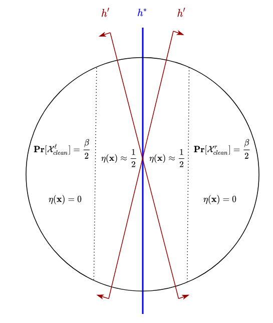
Figure 1: The geometry of our example; here $h^{*}$ represents the optimal classifier.

References

- Angluin and Laird (1987) Dana Angluin and Philip D. Laird. Learning from noisy examples. Mach. Learn., 2(4):343–370, 1987.
- Awasthi et al. (2014) Pranjal Awasthi, Maria-Florina Balcan, and Philip M. Long. The power of localization for efficiently learning linear separators with noise. In David B. Shmoys, editor, Symposium on Theory of Computing, STOC 2014, pages 449–458. ACM, 2014.
- Awasthi et al. (2015) Pranjal Awasthi, Maria-Florina Balcan, Nika Haghtalab, and Ruth Urner. Efficient learning of linear separators under bounded noise. In Peter Grünwald, Elad Hazan, and Satyen Kale, editors, Proceedings of The 28th Conference on Learning Theory, COLT 2015, volume 40 of JMLR Workshop and Conference Proceedings, pages 167–190. JMLR.org, 2015.
- Awasthi et al. (2016) Pranjal Awasthi, Maria-Florina Balcan, Nika Haghtalab, and Hongyang Zhang. Learning and 1-bit compressed sensing under asymmetric noise. In Vitaly Feldman, Alexander Rakhlin, and Ohad Shamir, editors, Proceedings of the 29th Conference on Learning Theory, COLT 2016, volume 49 of JMLR Workshop and Conference Proceedings, pages 152–192. JMLR.org, 2016.
- Bartlett et al. (2006) Peter L. Bartlett, Michael I. Jordan, and Jon D. Mcauliffe. Convexity, classification, and risk bounds. Journal of the American Statistical Association, 101(473):138–156, 2006.
- Blanchard et al. (2003) Gilles Blanchard, G´bor Lugosi, and Nicolas Vayatis. On the rate of convergence of regularized boosting classifiers. J. Mach. Learn. Res., 4:861–894, 2003. ISSN 1532-4435.
- Blum et al. (1994) Avrim Blum, Merrick L. Furst, Jeffrey C. Jackson, Michael J. Kearns, Yishay Mansour, and Steven Rudich. Weakly learning DNF and characterizing statistical query learning using fourier analysis. In Frank Thomson Leighton and Michael T. Goodrich, editors, Proceedings of the Twenty-Sixth Annual ACM Symposium on Theory of Computing, pages 253–262. ACM, 1994.
- Blum et al. (1996) Avrim Blum, Alan M. Frieze, Ravi Kannan, and Santosh S. Vempala. A polynomial-time algorithm for learning noisy linear threshold functions. In 37th Annual Symposium on Foundations of Computer Science, FOCS ’96, Burlington, Vermont, USA, 14-16 October, 1996, pages 330–338. IEEE Computer Society, 1996.
- Blum et al. (2003) Avrim Blum, Adam Kalai, and Hal Wasserman. Noise-tolerant learning, the parity problem, and the statistical query model. J. ACM, 50(4):506–519, July 2003.
- Boucheron et al. (2005) Stéphane Boucheron, Olivier Bousquet, and Gábor Lugosi. Theory of classification: a survey of some recent advances. ESAIM: Probability and Statistics, 9:323–375, 2005.
- Brodley and Friedl (1999) Carla E. Brodley and Mark A. Friedl. Identifying mislabeled training data. J. Artif. Intell. Res., 11:131–167, 1999.
- Bshouty and Feldman (2002) Nader H. Bshouty and Vitaly Feldman. On using extended statistical queries to avoid membership queries. J. Mach. Learn. Res., 2:359–395, March 2002.
- Bshouty et al. (1999) Nader H. Bshouty, Nadav Eiron, and Eyal Kushilevitz. PAC learning with nasty noise. In Osamu Watanabe and Takashi Yokomori, editors, Algorithmic Learning Theory, 10th International Conference, ALT ’99, volume 1720 of Lecture Notes in Computer Science, pages 206–218. Springer, 1999.
- Bylander (1994) Tom Bylander. Learning linear threshold functions in the presence of classification noise. In Proceedings of the Seventh Annual Conference on Computational Learning Theory, COLT ’94, page 340–347. Association for Computing Machinery, 1994.
- Chen et al. (2020) Sitan Chen, Frederic Koehler, Ankur Moitra, and Morris Yau. Classification under misspecification: Halfspaces, generalized linear models, and connections to evolvability. CoRR, abs/2006.04787, 2020.
- Cohen (1997) E. Cohen. Learning noisy perceptrons by a perceptron in polynomial time. In Proceedings 38th Annual Symposium on Foundations of Computer Science, pages 514–523, 1997.
- Daniely (2015) Amit Daniely. A PTAS for agnostically learning halfspaces. In Peter Grünwald, Elad Hazan, and Satyen Kale, editors, Proceedings of The 28th Conference on Learning Theory, COLT 2015, volume 40 of JMLR Workshop and Conference Proceedings, pages 484–502. JMLR.org, 2015.
- Daniely (2016) Amit Daniely. Complexity theoretic limitations on learning halfspaces. In Daniel Wichs and Yishay Mansour, editors, Proceedings of the 48th Annual ACM SIGACT Symposium on Theory of Computing, STOC 2016, pages 105–117. ACM, 2016.
- Dawid and Skene (1979) A. P. Dawid and A. M. Skene. Maximum likelihood estimation of observer error-rates using the em algorithm. Journal of the Royal Statistical Society. Series C (Applied Statistics), 28(1):20–28, 1979.
- Decatur (1993) Scott E. Decatur. Statistical queries and faulty PAC oracles. In Lenny Pitt, editor, Proceedings of the Sixth Annual ACM Conference on Computational Learning Theory, COLT 1993, pages 262–268. ACM, 1993.
- Decatur (1996) Scott E. Decatur. Learning in Hybrid Noise Environments Using Statistical Queries, pages 259–270. Springer New York, 1996.
- Decatur and Gennaro (1995) Scott E. Decatur and Rosario Gennaro. On learning from noisy and incomplete examples. In Wolfgang Maass, editor, Proceedings of the Eigth Annual Conference on Computational Learning Theory, COLT 1995, Santa Cruz, California, USA, July 5-8, 1995, pages 353–360. ACM, 1995.
- Diakonikolas et al. (2019) Ilias Diakonikolas, Themis Gouleakis, and Christos Tzamos. Distribution-independent PAC learning of halfspaces with massart noise. In Hanna M. Wallach, Hugo Larochelle, Alina Beygelzimer, Florence d’Alché-Buc, Emily B. Fox, and Roman Garnett, editors, Advances in Neural Information Processing Systems 32: Annual Conference on Neural Information Processing Systems 2019, pages 4751–4762, 2019.
- Diakonikolas et al. (2020a) Ilias Diakonikolas, Daniel M. Kane, Vasilis Kontonis, Christos Tzamos, and Nikos Zarifis. A polynomial time algorithm for learning halfspaces with tsybakov noise, 2020a.
- Diakonikolas et al. (2020b) Ilias Diakonikolas, Vasilis Kontonis, Christos Tzamos, and Nikos Zarifis. Learning halfspaces with massart noise under structured distributions. CoRR, abs/2002.05632, 2020b.
- Diakonikolas et al. (2020c) Ilias Diakonikolas, Vasilis Kontonis, Christos Tzamos, and Nikos Zarifis. Learning halfspaces with tsybakov noise. CoRR, abs/2006.06467, 2020c.
- Feldman et al. (2006) V. Feldman, P. Gopalan, S. Khot, and A. K. Ponnuswami. New results for learning noisy parities and halfspaces. In 2006 47th Annual IEEE Symposium on Foundations of Computer Science (FOCS’06), pages 563–574, 2006.
- Feldman (2008) Vitaly Feldman. Evolvability from learning algorithms. In Cynthia Dwork, editor, Proceedings of the 40th Annual ACM Symposium on Theory of Computing, 2008, pages 619–628. ACM, 2008.
- Feldman (2009) Vitaly Feldman. Robustness of evolvability. In COLT 2009 - The 22nd Conference on Learning Theory, 2009.
- Feldman (2011) Vitaly Feldman. Distribution-independent evolvability of linear threshold functions. In Sham M. Kakade and Ulrike von Luxburg, editors, COLT 2011 - The 24th Annual Conference on Learning Theory, June 9-11, 2011, volume 19 of JMLR Proceedings, pages 253–272. JMLR.org, 2011.
- Frénay and Verleysen (2014) Benoît Frénay and Michel Verleysen. Classification in the presence of label noise: A survey. IEEE Trans. Neural Networks Learn. Syst., 25(5):845–869, 2014.
- Freund (1999) Yoav Freund. An adaptive version of the boost by majority algorithm. In Shai Ben-David and Philip M. Long, editors, Proceedings of the Twelfth Annual Conference on Computational Learning Theory, COLT 1999, pages 102–113. ACM, 1999.
- Friedman et al. (2000) Jerome Friedman, Trevor Hastie, and Robert Tibshirani. Additive logistic regression: a statistical view of boosting. Ann. Statist., 28(2):337–407, 04 2000.
- Ganapathiraju and Picone (2000) Aravind Ganapathiraju and Joseph Picone. Support vector machines for automatic data cleanup. In Sixth International Conference on Spoken Language Processing, ICSLP 2000 / INTERSPEECH 2000, pages 210–213. ISCA, 2000.
- Guruswami and Raghavendra (2006) V. Guruswami and P. Raghavendra. Hardness of learning halfspaces with noise. In 2006 47th Annual IEEE Symposium on Foundations of Computer Science (FOCS’06), pages 543–552, 2006.
- Hanneke and Yang (2015) Steve Hanneke and Liu Yang. Minimax analysis of active learning. J. Mach. Learn. Res., 16(1):3487–3602, January 2015.
- Haussler (1992) David Haussler. Decision theoretic generalizations of the pac model for neural net and other learning applications. Information and Computation, 100(1):78 – 150, 1992.
- Hoeffding (1963) Wassily Hoeffding. Probability inequalities for sums of bounded random variables. Journal of the American Statistical Association, 58(301):13–30, 1963.
- Kalai et al. (2008) Adam Tauman Kalai, Adam R. Klivans, Yishay Mansour, and Rocco A. Servedio. Agnostically learning halfspaces. SIAM J. Comput., 37(6):1777–1805, 2008.
- Kanade et al. (2010) Varun Kanade, Leslie G. Valiant, and Jennifer Wortman Vaughan. Evolution with drifting targets. In Adam Tauman Kalai and Mehryar Mohri, editors, COLT 2010 - The 23rd Conference on Learning Theory, pages 155–167. Omnipress, 2010.
- Kearns (1998) Michael Kearns. Efficient noise-tolerant learning from statistical queries. J. ACM, 45(6):983–1006, November 1998.
- Kearns et al. (1992) Michael J. Kearns, Robert E. Schapire, and Linda Sellie. Toward efficient agnostic learning. In David Haussler, editor, Proceedings of the Fifth Annual ACM Conference on Computational Learning Theory, COLT 1992, pages 341–352. ACM, 1992.
- Khardon and Wachman (2007) Roni Khardon and Gabriel Wachman. Noise tolerant variants of the perceptron algorithm. J. Mach. Learn. Res., 8:227–248, 2007.
- Koltchinskii (2006) Vladimir Koltchinskii. Local rademacher complexities and oracle inequalities in risk minimization. Ann. Statist., 34(6):2593–2656, 12 2006.
- Laird (1988) Philip D. Laird. Learning from Good and Bad Data. Kluwer Academic Publishers, USA, 1988.
- Li and Long (1999) Yi Li and Philip M. Long. The relaxed online maximum margin algorithm. In Sara A. Solla, Todd K. Leen, and Klaus-Robert Müller, editors, Advances in Neural Information Processing Systems 12, [NIPS Conference, Denver, Colorado, USA, November 29 - December 4, 1999], pages 498–504. The MIT Press, 1999.
- Lin and Wang (2004) Chun-fu Lin and Sheng-De Wang. Training algorithms for fuzzy support vector machines with noisy data. Pattern Recognit. Lett., 25(14):1647–1656, 2004.
- Malossini et al. (2006) Andrea Malossini, Enrico Blanzieri, and Raymond T. Ng. Detecting potential labeling errors in microarrays by data perturbation. Bioinformatics, 22(17):2114–2121, 06 2006.
- Mammen and Tsybakov (1999) Enno Mammen and Alexandre B. Tsybakov. Smooth discrimination analysis. Ann. Statist., 27(6):1808–1829, 12 1999.
- Manwani and Sastry (2013) Naresh Manwani and P. S. Sastry. Noise tolerance under risk minimization. IEEE Trans. Cybern., 43(3):1146–1151, 2013.
- Massart and Nédélec (2006) Pascal Massart and Élodie Nédélec. Risk bounds for statistical learning. Ann. Statist., 34(5):2326–2366, 10 2006.
- Morel et al. (2007) J.M. Morel, P. Massart, J. Picard, F. Takens, and B. Teissier. Concentration Inequalities and Model Selection: Ecole D’Eté de Probabilités de Saint-Flour XXXIII - 2003. Springer, 2007.
- Rosenblatt (1958) F. Rosenblatt. The perceptron: a probabilistic model for information storage and organization in the brain. Psychological review, 65(6):386–408, 1958.
- Sloan (1988) Robert Sloan. Types of noise in data for concept learning. In Proceedings of the First Annual Workshop on Computational Learning Theory, COLT ’88, page 91–96. Morgan Kaufmann Publishers Inc., 1988.
- Sloan (1992) Robert H. Sloan. Corrigendum to types of noise in data for concept learning. In Proceedings of the Fifth Annual Workshop on Computational Learning Theory, COLT ’92, page 450. Association for Computing Machinery, 1992.
- Smyth (1996) Padhraic Smyth. Bounds on the mean classification error rate of multiple experts. Pattern Recogn. Lett., 17(12):1253–1257, 1996.
- Smyth et al. (1994) Padhraic Smyth, Usama Fayyad, Michael Burl, Pietro Perona, and Pierre Baldi. Inferring ground truth from subjective labelling of venus images. In Proceedings of the 7th International Conference on Neural Information Processing Systems, NIPS’94, page 1085–1092. MIT Press, 1994.
- Tsybakov (2004) Alexandre B. Tsybakov. Optimal aggregation of classifiers in statistical learning. The Annals of Statistics, 32(1):135–166, 2004.
- Valiant (1985) L. G. Valiant. Learning disjunction of conjunctions. In Proceedings of the 9th International Joint Conference on Artificial Intelligence - Volume 1, IJCAI’85, page 560–566. Morgan Kaufmann Publishers Inc., 1985. ISBN 0934613028.
- Valiant (1984) Leslie G. Valiant. A theory of the learnable. In Richard A. DeMillo, editor, Proceedings of the 16th Annual ACM Symposium on Theory of Computing, pages 436–445. ACM, 1984.
- Valiant (2009) Leslie G. Valiant. Evolvability. J. ACM, 56(1):3:1–3:21, 2009.
- van den Hout and van der Heijden (2002) Ardo van den Hout and Peter G. M. van der Heijden. Randomized response, statistical disclosure control and misclassification: A review. International Statistical Review / Revue Internationale de Statistique, 70(2):269–288, 2002.
- Yan and Zhang (2017) Songbai Yan and Chicheng Zhang. Revisiting perceptron: Efficient and label-optimal learning of halfspaces. In I. Guyon, U. V. Luxburg, S. Bengio, H. Wallach, R. Fergus, S. Vishwanathan, and R. Garnett, editors, Advances in Neural Information Processing Systems 30, pages 1056–1066. Curran Associates, Inc., 2017.
- Zhang et al. (2020) Chicheng Zhang, Jie Shen, and Pranjal Awasthi. Efficient active learning of sparse halfspaces with arbitrary bounded noise. CoRR, abs/2002.04840, 2020.
- Zhang et al. (2017) Yuchen Zhang, Percy Liang, and Moses Charikar. A hitting time analysis of stochastic gradient langevin dynamics. volume 65 of Proceedings of Machine Learning Research, pages 1980–2022. PMLR, 07–10 Jul 2017.