A Framework for Multiphase Galactic Wind Launching using TIGRESS

Abstract

Galactic outflows have density, temperature, and velocity variations at least as large as that of the multiphase, turbulent interstellar medium (ISM) from which they originate. We have conducted a suite of parsec-resolution numerical simulations using the TIGRESS framework, in which outflows emerge as a consequence of interaction between supernovae (SNe) and the star-forming ISM. The outflowing gas is characterized by two distinct thermal phases, cool ($T\lesssim 10^{4}$ K) and hot ($T\gtrsim 10^{6}$ K), with most mass carried by the cool phase and most energy and newly-injected metals carried by the hot phase. Both components have a broad distribution of outflow velocity, and especially for cool gas this implies a varying fraction of escaping material depending on the halo potential. Informed by the TIGRESS results, we develop straightforward analytic formulae for the joint probability density functions (PDFs) of mass, momentum, energy, and metal loading as distributions in outflow velocity and sound speed. The model PDFs have only two parameters, SFR surface density $\Sigma_{\rm SFR}$ and the metallicity of the ISM, and fully capture the behavior of the original TIGRESS simulation PDFs over $\Sigma_{\rm SFR}\in(10^{-4},1)\,M_{\odot}\,{\rm kpc}^{-2}\,{\rm yr}^{-1}$. Employing PDFs from resolved simulations will enable galaxy formation subgrid model implementations with wind velocity and temperature (as well as total loading factors) that are based on theoretical predictions rather than empirical tuning. This is a critical step to incorporate advances from TIGRESS and other high-resolution simulations in future cosmological hydrodynamics and semi-analytic galaxy formation models. We release a python package to prototype our model and to ease its implementation.

1 Introduction

Galactic scale outflows are prevalent in observations of star forming galaxies (e.g., 2005ARA&A..43..769V; 2018Galax...6..138R, for reviews) and play a central role in contemporary theory of galaxy formation and evolution (e.g., 2015ARA&A..53...51S; 2017ARA&A..55...59N, for reviews). Although single-phase outflows have often been adopted in cosmological subgrid models (e.g., 2003MNRAS.339..289S; 2006MNRAS.373.1265O; 2013MNRAS.436.3031V), real galactic outflows are clearly multiphase in nature (2020A&ARv..28....2V, for a recent review). Multiwavelength observations of fast-moving gas include radio lines from cold molecular and atomic outflows (e.g., 2015ApJ...814...83L; 2018ApJ...856...61M), optical and UV absorption lines from warm ionized outflows (e.g., 2000ApJS..129..493H; 2005ApJ...621..227M; 2015ApJ...809..147H; 2016MNRAS.457.3133C; 2017MNRAS.469.4831C), and X-rays from hot ionized outflows (e.g., 1999ApJ...523..575L; 2004ApJS..151..193S). Furthermore, numerical simulations that resolve the multiphase ISM in galaxies and include supernova (SN) feedback (e.g., 2012MNRAS.421.3522H; 2017MNRAS.466.1903G; 2017ApJ...841..101L; 2018ApJ...853..173K; 2019MNRAS.483.3363H; 2020ApJ...895...43S) show that both warm/cold and hot gas in the ISM are driven out together by superbubble expansion and breakout. Thus, launching of multiphase outflows appears to be the generic outcome of SN feedback in star-forming galaxies.

In 2020arXiv200616315K, we analyzed the outflows in a suite of parsec-resolution numerical simulations spanning a range of star-forming galaxy environments. We separated out two distinct thermal phases at $T<2\times 10^{4}\,{\rm K}$ (cool) and $T>5\times 10^{5}\,{\rm K}$ (hot) with a subdominant intermediate phase at temperatures in between. For each phase, we characterized horizontally-integrated mass, momentum, energy, and metal fluxes and loading factors (fluxes normalized by the corresponding star formation rate (SFR), or by the SN momentum, energy, and metal injection rate). We also measured horizontally averaged mean velocities of each outflow phase. In agreement with our previous study for solar neighborhood conditions (2018ApJ...853..173K), 2020arXiv200616315K showed that for all the environments investigated, (1) hot outflows deliver energy and SN-injected metals at high velocity to the circumgalactic medium (CGM); and (2) cool outflows carry much more mass, but at much lower velocity. We presented scaling relations for the dependence of multiphase outflow properties on the SFR, midplane pressure, and weight of the ISM, which are all (equally) good predictors for the mean outflow properties.

The characterization of 2020arXiv200616315K addressed fundamental quantitative questions: how different are mass, momentum, energy, and metal outflow rates in different thermal phases? How do outflow rates scale with galactic conditions? However, in distilling “velocity-integrated” properties, important information regarding velocity and thermal distributions is lost. In particular, the cool-gas velocity distribution typically has an exponential wing extending to high velocity (2018ApJ...853..173K; 2020ApJ...894...12V), such that significant cool ISM material could escape into the CGM region even if the mean cool outflow velocity is lower than a galaxy’s escape speed.

Here we investigate the full joint probability distribution function (PDF) of outflow velocity and sound speed. We begin by showing that given a mass loading PDF, the momentum, energy, and metal loading PDFs can be constructed (Section 2). We then develop a simple, parameterized model for the mass loading, with separate analytic functions describing cool and hot PDFs. These PDFs are combined with the scaling relations presented in 2020arXiv200616315K to create an easy-to-use outflow launching model (Section 3), which can be implemented in either semi-analytic or fully numerical cosmological models of galaxy formation. We provide a python package Twind for model PDFs and sampling, and demonstrate its application (Section 4 and LABEL:sec:appendix_twind).

It should be borne in mind that the particular set of TIGRESS models we employ have several advantages, but also come with caveats, as discussed below. Thus, we consider the main goal of this Letter to be a proof of principle: we show that joint PDFs of outflow velocity and sound speed are an efficient yet accurate way to encapsulate complex outflow properties from multi-physics, high-resolution simulations. We further show that an analytic model representation of the joint PDFs enables immediate and practical application of the results from small scale simulations to cosmological simulations and semi-analytic models. While the demonstration employs our current TIGRESS simulation suite, results from other simulations (with additional physics, and/or a wider parameter space) could be used in a similar fashion, fitting to obtain functional forms and parameters that characterize outflow PDFs based on kpc-scale galactic properties.

2 Joint PDFs of outflow velocity and sound speed

We use a suite of local galactic disk models simulated with the TIGRESS framework (2017ApJ...846..133K), as presented in 2020arXiv200616315K. The suite is comprised of 7 models, representing the range of galactic properties in nearby Milky Way-like star-forming galaxies, as summarized in Table 1. The self-regulated disk properties cover a wide range of SFR surface density ($\Sigma_{\rm SFR}\sim 10^{-4}-1\,M_{\odot}\,{\rm kpc}^{-2}\,{\rm yr}^{-1}$), gas surface density ($\Sigma_{\rm gas}\sim 1-100\,M_{\odot}\,{\rm pc^{-2}}$), and total midplane pressure/weight ($P_{\rm mid},\mathcal{W}\sim 10^{3}-10^{6}\,k_{B}\,{\rm cm}^{-3}\,{\rm K}$). We refer the reader to 2020arXiv200616315K for full descriptions of models and methods (a brief summary can be found in Appendix A).

We note here that stellar feedback processes considered in the TIGRESS framework include grain photoelectric heating by FUV radiation (without explicit radiation transfer) and SNe from star clusters and runaway OB stars, while other feedback processes including radiation pressure, photoionization, stellar winds, and cosmic rays are neglected. The missing feedback processes may affect the total outflow rates and distributions directly because some wind-driving forces such as cosmic ray and ionized-gas pressure gradients (e.g., 2018MNRAS.479.3042G; 2018ApJ...865L..22E) are not represented, and/or indirectly, because early feedback might reduce clustering of star formation and SNe (e.g., 2020MNRAS.491.3702H), which are known to enhance outflows (e.g., 2018MNRAS.481.3325F). We note that the effects of ‘‘early’’ feedback has explicitly been shown to be significant in dwarfs (2018ApJ...865L..22E; 2020arXiv200911309S), but is not yet fully demonstrated in Milky Way-like conditions as simulated in the TIGRESS suite. Also, the particular treatments in the TIGRESS framework for star formation using sink particles and SNe could potentially affect the properties of outflows (see 2018ApJ...853..173K and 2020arXiv200616315K for in-depth discussions). New metals (as opposed to the metals in the initial disk) in our simulations are injected only by SNe as we do not model stellar winds, which may affect the metallicity of outflows.

The above caveats and particularities certainly affect our specific quantitative results, but the overall approach we propose is quite general as a way to represent the mass, momentum, energy, and metals launched in multiphase outflows.

We now turn to distributions of outflowing gas in the TIGRESS suite. Let $f_{q}(u,w;z)$ be the PDF of an outflow quantity $q$ at a given height $z$ within logarithmic velocity bins of vertical outgoing velocity $u\equiv{\rm log_{\small 10}}v_{\rm out}$ and sound speed $w\equiv{\rm log_{\small 10}}c_{s}$:

$$f_{q}(u,w;z)\equiv\frac{1}{\left\langle{q(z)}\right\rangle}\frac{d^{2}q(z)}{dudw}.$$ (1)

Here, $f_{q}$ is in units of dex${}^{-2}$, $q(z)$ is a quantity defined at height $z$ over the entire $x$-$y$ horizontal domain and the time interval $t\in(t_{1},t_{2})$ of interest, and $\left\langle{q(z)}\right\rangle$ is the temporal and horizontal average of $q$ (also summed over all $u$ and $w$) so that the time averaged PDF has unit normalization, $\int f_{q}dudw=1$. The physical quantities $q$ of interest are vertical out-going fluxes

$$\mathcal{F}_{M}=\rho v_{\rm out} \quad\textrm{(mass flux)},$$ (2)

$$\mathcal{F}_{p}=\rho v_{\rm out}^{2}+P+\Pi_{B} \quad\textrm{($z$-momentum flux)},$$ (3)

$$\mathcal{F}_{E}=\rho v_{\rm out}v_{\mathcal{B}}^{2}/2+\mathcal{S}_{z} \quad\textrm{(energy flux)},$$ (4)

$$\mathcal{F}_{Z}=\rho Zv_{\rm out} \quad\textrm{(metal flux)}.$$ (5)

Here, $v_{\rm out}\equiv v_{z}{\rm sgn}(z)$ is the vertical outgoing velocity,

$$\Pi_{B}\equiv\frac{B^{2}}{8\pi}-\frac{B_{z}^{2}}{4\pi}$$ (6)

is the vertical component of the Maxwell stress (magnetic pressure + tension),

$$v_{\mathcal{B}}\equiv\left({v^{2}+\frac{2\gamma}{\gamma-1}c_{s}^{2}}\right)^{1/2}$$ (7)

is the Bernoulli velocity, where we use isothermal sound speed $c_{s}^{2}\equiv P/\rho$, and

$$\mathcal{S}_{z}\equiv\frac{\left({v_{\rm out}B^{2}-B_{\rm out}\mathbf{v}\cdot\mathbf{B}}\right)}{4\pi}$$ (8)

is the vertical component of the Poynting flux with the vertical outgoing magnetic field $B_{\rm out}=B_{z}{\rm sgn}(z)$, and $Z$ is metallicity as traced by passive scalars in the MHD simulations. Note that we adopt $\gamma=5/3$ so that $2\gamma/(\gamma-1)=5$. In the outflow analysis of 2020arXiv200616315K, we did not include magnetic terms in momentum and energy fluxes; Equation 3 and Equation 4 include them for completeness but here we show they may be neglected.

The procedure to calculate the joint PDFs is as follows: we (1) extract one-zone thick slices at a distance from the midplane $|z|$ for both upper and lower sides (either fixed heights at $z=\pm 500\,{\rm pc}$ and $\pm 1\,{\rm kpc}$ or time-varying heights at $z=\pm H$ and $\pm 2H$, where $H$ is the instantaneous gas scale height) over $0.5<t/t_{\rm orb}<1.5$, (2) sum up each quantity within square bins $du=dw=0.02$ dex, and (3) normalize each PDF with the total ‘‘outflowing’’ quantity ($v_{\rm out}>0$) averaged over the time range of interest at a given height defined by

$$\left\langle{q(z_{k})}\right\rangle\equiv\frac{\sum_{n,i,j}q(x_{i},y_{j},t_{n};z_{k})\Theta(v_{\rm out}>0)}{N_{x}N_{y}N_{t}},$$ (9)

where $\Theta(C)$ is the top-hat-like filter that returns 1 if the conditional argument is true or 0 otherwise, $N_{x}$ and $N_{y}$ are the numbers of grid zones in the horizontal directions, and $N_{t}$ is number of snapshots analyzed. In 2020arXiv200616315K, we use $\overline{q}(z;t)$ to denote the horizontally-integrated/averaged quantities that are outflowing $v_{\rm out}>0$ (with a phase separation if needed) at a given time. Thus, $\left\langle{q}\right\rangle$ here is simply the time-average of the corresponding $\overline{q}$, which is presented in Table 3 of 2020arXiv200616315K and available online at doi:10.5281/zenodo.3872049.

In addition to the total metal flux, it is of interest to quantify how enriched the outflow is compared to the ISM. To derive the distribution of the outflow enrichment factor, we first define the average metallicity within each logarithmic velocity bin as

$$Z(u,w;z)\equiv\frac{\left\langle{\mathcal{F}_{Z}(z)}\right\rangle}{\left\langle{\mathcal{F}_{M}(z)}\right\rangle}\frac{f_{\mathcal{F}_{Z}}(u,w;z)}{f_{\mathcal{F}_{M}}(u,w;z)}.$$ (10)

so that the corresponding enrichment factor is

$$\zeta(u,w;z)\equiv\frac{Z(u,w;z)}{Z_{\rm ISM}}.$$ (11)

The mean ISM metallicity $Z_{\rm ISM}$ is obtained by taking the time average of the instantaneous ISM metallicity $\overline{Z}_{\rm ISM}(t)$ defined by the mean metallicity of the cool phase within $|z|<50\,{\rm pc}$ (see Section 4.2 of 2020arXiv200616315K).

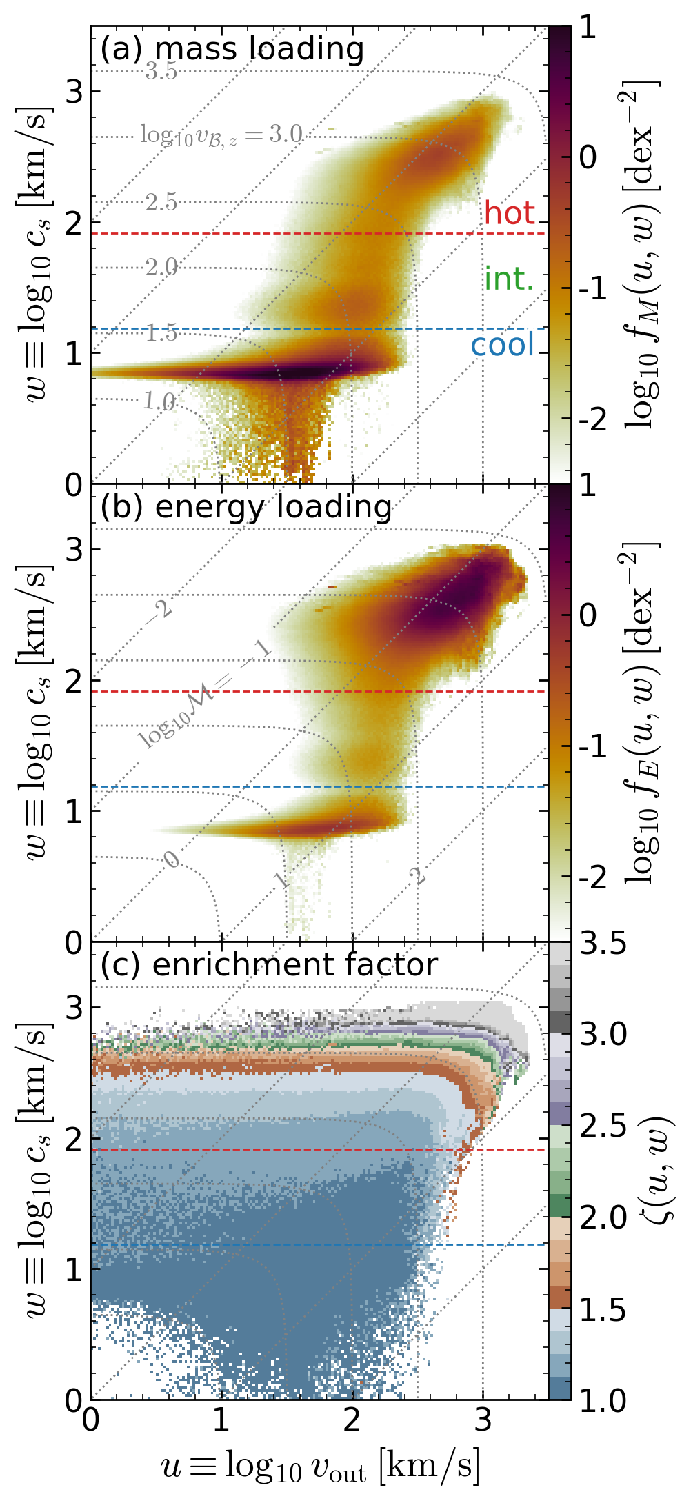
Figure 1: Joint PDFs in ${\rm log_{\small 10}}v_{\rm out}$ and ${\rm log_{\small 10}}c_{s}$ for model R4 ($\Sigma_{\rm gas}\sim 30\,M_{\odot}\,{\rm pc^{-2}}$ and $\Sigma_{\rm SFR}\sim 10^{-1}\,M_{\odot}\,{\rm kpc}^{-2}\,{\rm yr}^{-1}$) at $|z|=H$. (a) Mass loading PDF, (b) energy loading PDF, and (c) enrichment factor distribution. The red and blue dashed lines denote temperature cuts to separate cool ($T<2\times 10^{4}\,{\rm K}$), intermediate ($2\times 10^{4}\,{\rm K}<T<5\times 10^{5}\,{\rm K}$), and hot ($5\times 10^{5}\,{\rm K}<T$) phases. The dotted gray lines denote loci of constant $v_{\mathcal{B},z}\equiv(v_{\rm out}^{2}+5c_{s}^{2})^{1/2}$ (labeled in (a)) and $\mathcal{M}\equiv v_{\rm out}/c_{s}$ (labeled in (b)); loci are identical in all panels.

To make our approach more general, we translate our results into loading factors, defined by ratios of outflow fluxes to corresponding areal rates of star formation (and related areal rates) in our simulations. This translation eases the connection to global simulations, in which e.g. the mass loading factor from a given cell represents the wind mass loss rate relative to SFR in that cell. We note that $\Sigma_{\rm SFR}$ is still needed for our model parameterization; in global models appropriate projection and averaging may be used to define $\Sigma_{\rm SFR}$ in the region centered on a given cell (of arbitrary shape).

Following 2020arXiv200616315K, we define

$$\eta_{q}(x,y,t;z)=\frac{\mathcal{F}_{q}(x,y,t;z)}{\left\langle{q_{\rm ref}\Sigma_{\rm SFR}/m_{*}}\right\rangle}.$$ (12)

Here, $q=M$, $p$, $E$, and $Z$ as in Equation 2 -- Equation 5, $m_{*}$ is the mass of new stars formed per SN, and the reference values per SN event for mass, momentum, energy, and metal mass are

$$M_{\rm ref}=m_{*} =95.5\,M_{\odot},$$ (13)

$$p_{\rm ref}=E_{\rm SN}/(2v_{\rm cool}) =1.25\times 10^{5}\,M_{\odot}\,{\rm km}\,{\rm s}^{-1},$$ (14)

$$E_{\rm ref}=E_{\rm SN} =10^{51}\,{\rm erg},$$ (15)

$$Z_{\rm ref}\equiv M_{\rm ej}Z_{\rm SN} =2\,M_{\odot}.$$ (16)

These values are adopted based on a 2001MNRAS.322..231K initial mass function, with ejecta mass $M_{\rm ej}=10\,M_{\odot}$, and metallicity $Z_{\rm SN}=0.2$ from STARBURST99 (1999ApJS..123....3L). We choose $v_{\rm cool}=200\,{\rm km}\,{\rm s}^{-1}$ (see Section 4.1 of 2020arXiv200616315K for the full discussion of this choice and $p_{\rm ref}$). With these definitions, $\eta_{M}$ is the ratio of mass outflow rate to SFR, $\eta_{E}$ ($\eta_{Z}$) is the ratio of energy outflow rate (metal mass outflow rate) to SN energy (SN metal mass) injection rate, and $\eta_{p}$ is the ratio of z-momentum outflow rate to the vertical momentum injection rate from post-Sedov-stage SNe. Note that the PDFs are identical for fluxes and loading factors as they differ by a constant factor and are normalized to be integrated to 1. Therefore $f_{q}$ with $q=M$, $p$, $E$, and $Z$ may denote either a flux PDF or loading PDF. We note also that loading factors may be defined for all material in the outflow or separated by thermal phase, depending on whether the corresponding flux is for all material or phase-separated (see 2020arXiv200616315K).

Figure 1 shows (a) the mass loading PDF ($f_{M}(u,w)$), (b) the energy loading PDF ($f_{E}(u,w)$), and (c) the metal enrichment factor ($\zeta(u,w)$) for model R4 at $|z|=H$. As reported in 2020arXiv200616315K (see also 2018ApJ...853..173K), it is evident that the cool outflow carries most of the mass (panel a), while the hot outflow carries most of the energy (panel b) and metals (panel c). In addition, Figure 1(b) clearly shows a wide distribution in $v_{\rm out}$ (with a narrow spread in $c_{s}$) for the cool outflow, contrasting in Figure 1(a) with a broader distribution along both axes for the hot outflow. This makes plain that naively adopting a single characteristic velocity and temperature would poorly represent both the mass and energy outflow rates.

For reference, Figure 1 includes contours of constant $v_{\mathcal{B},z}$, where the outflowing component of the Bernoulli velocity is defined as

$$v_{\mathcal{B},z}\equiv(v_{\rm out}^{2}+5c_{s}^{2})^{1/2}.$$ (17)

To gauge whether fluid elements with given $(u,w)$ have sufficient energy to travel from the launching place to a distant location, $v_{\mathcal{B},z}$ can be compared to the escape velocity $v_{\rm esc}$ (which can be defined via the gravitational potential difference between wind launching position and the distant point).

For outflows driven under conditions like model R4 (with $\Sigma_{\rm SFR}\sim 0.1\,M_{\odot}\,{\rm kpc}^{-2}\,{\rm yr}^{-1}$), most hot outflows would escape the main galaxy if $v_{\rm esc}\lesssim 300\,{\rm km}\,{\rm s}^{-1}$, delivering significant energy and metal fluxes far into the CGM. Cool outflows in a massive galaxy would, however, fall back as fountains. In the case of a low-mass galaxy with a shallow halo potential, e.g., $v_{\rm esc}<50\,{\rm km}\,{\rm s}^{-1}$, cool outflows would carry significant mass outside the main galaxy into the CGM, at the same time as the hot wind carries energy and momentum.

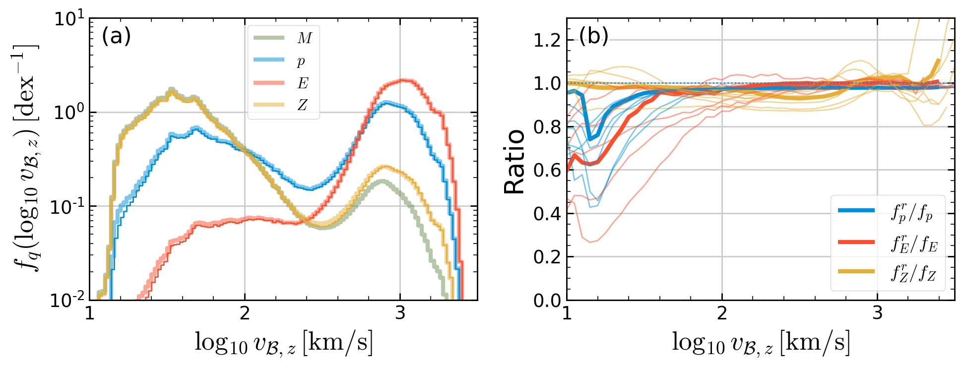
Figure 2: (a) Examples of PDFs for loading factors projected onto ${\rm log_{\small 10}}v_{\mathcal{B},z}$ for model R4 at $|z|=H$. Thick lines show direct measurements of all PDFs, while thin lines with the same color (overlying the thick lines almost everywhere) show reconstructions from the mass PDF of momentum (Equation 19), energy (Equation 21), and metal (Equation 22) PDFs. (b) The ratios of reconstructed PDFs to the original PDFs for all models at $|z|=H$. The mean ratio at a given ${\rm log_{\small 10}}v_{\mathcal{B},z}$ is obtained by a mass flux weighted average. (Thick lines correspond to model R4, shown to left.)

Figure 1(c) demonstrates that the enrichment factor is tightly related to $v_{\mathcal{B},z}$. This relation is rooted in the strong correlation between energy and SN-origin metal loading factors of the hot outflow seen in Figure 15 of 2020arXiv200616315K (see also 2015ApJ...800L...4C; 2020ApJ...890L..30L). We find that the model

$$\tilde{\zeta}=\left({\frac{v_{\mathcal{B},z}}{3.2\times 10^{3}\,{\rm km}\,{\rm s}^{-1}}}\right)^{1.7}\left[{\frac{Z_{\rm SN}}{Z_{\rm ISM}}-1}\right]+1,$$ (18)

for the enrichment factor defined in Equation 11 is in good agreement with the results for all heights ($|z|=H$, $2H$, 500 pc, and 1 kpc) where we measure the outflow properties from the full TIGRESS suite. As a result, for a given $Z_{\rm ISM}$, model outflow metallicity $\tilde{Z}\equiv\tilde{\zeta}Z_{\rm ISM}$ increases with the specific energy (or $v_{\mathcal{B},z}$) at high-$v_{\mathcal{B},z}$ and flattens to $Z_{\rm ISM}$ at low-$v_{\mathcal{B},z}$. This formula predicts that, even in the limit of zero ISM metallicity (although this is outside the parameter space we explored), the hot outflow at high-$v_{\mathcal{B}}$ would have large non-zero metallicity $\tilde{Z}\propto Z_{\rm SN}v_{\mathcal{B},z}^{1.7}$ derived from very recent SN ejecta. Note that Equation 18 uses $v_{\mathcal{B},z}$ which can be directly calculated from $u$ and $w$. 2020arXiv200616315K found a slight enrichment of the cool outflow ($\sim 10\%$ at the largest $\Sigma_{\rm SFR}\sim 1\,M_{\odot}\,{\rm kpc}^{-2}\,{\rm yr}^{-1}$), but we neglect it for simplicity. In Equation 18, $\tilde{\zeta}\rightarrow 1$ for low $v_{\mathcal{B},z}$, so the outflow metallicity model is valid for cool gas, in which $\tilde{Z}$ approaches $Z_{\rm ISM}$.

Under a certain set of assumptions, the momentum, energy, and metal loading PDFs can be recovered from the mass loading PDFs. If magnetic terms are negligible (and the bin size of PDFs is sufficiently small), the momentum loading PDF can be reconstructed from $f_{M}$ as

$$f_{p}^{r}\equiv\frac{\left\langle{\eta_{M}}\right\rangle}{\left\langle{\eta_{p}}\right\rangle}\frac{v_{\rm out}^{2}+c_{s}^{2}}{v_{p}v_{\rm out}}f_{M},$$ (19)

where $v_{p}\equiv p_{\rm ref}/M_{\rm ref}=1.3\times 10^{3}\,{\rm km}\,{\rm s}^{-1}$. The energy loading PDF can also be approximately reconstructed if the vertical component of kinetic energy dominates over the transverse component. In practice, there is non-negligible contribution from the transverse component of kinetic energy, but we find we can correct for this. Our model results are consistent with a simple bias factor that describes the ratio of outflow component to total specific energy as a function of $v_{\mathcal{B},z}$:

$$b\equiv\frac{v_{\mathcal{B},z}^{2}}{v_{\mathcal{B}}^{2}}=0.1{\rm log_{\small 10}}v_{\mathcal{B},z}+0.6,$$ (20)

for $v_{\mathcal{B},z}$ in units of km/s and $v_{\mathcal{B},z}\in(1,10^{4})\,{\rm km}\,{\rm s}^{-1}$. We then obtain the reconstructed energy loading PDF from the mass loading PDF as

$$f_{E}^{r}\equiv\frac{\left\langle{\eta_{M}}\right\rangle}{\left\langle{\eta_{E}}\right\rangle}\frac{1}{2}\frac{v_{\mathcal{B},z}^{2}}{v_{E}^{2}}\frac{f_{M}}{b},$$ (21)

where $v_{E}\equiv(E_{\rm ref}/M_{\rm ref})^{1/2}=7.3\times 10^{2}\,{\rm km}\,{\rm s}^{-1}$. Similarly, the metal loading PDF can be recovered using Equation 18 as

$$f_{Z}^{r}\equiv\frac{\left\langle{\eta_{M}}\right\rangle}{\left\langle{\eta_{Z}}\right\rangle}\frac{Z_{\rm ISM}}{Z_{e}}\tilde{\zeta}(v_{\mathcal{B},z})f_{M},$$ (22)

where $Z_{e}\equiv Z_{\rm ref}/M_{\rm ref}\rightarrow 0.02$.

To demonstrate how well PDFs for other variables can be recovered from the mass loading PDF with Equations (19), (21), and (22), Figure 2(a) plots the original PDFs projected onto the ${\rm log_{\small 10}}\,v_{\mathcal{B},z}$ axis (thick lines), in comparison with the reconstructed PDFs (thin lines), for model R4 at $|z|=H$. The reconstruction is successful: the thin lines are barely seen as they overlie the thick lines almost everywhere. For more quantitative comparison, Figure 2(b) plots the ratios between reconstructed and original PDFs for all models at $|z|=H$ (thick lines are for R4 and thin lines for other models). Again, the recovery of all PDFs is quite good, especially at $v_{\mathcal{B},z}$ larger than a few tens of km/s (which is what matters in the outflow context). This justifies the general assumption that the magnetic stress is not important in outflows and confirms the validity of the enrichment factor model (Equation 18) and the bias factor (Equation 20) for all cases.

3 Model PDFs and Validation

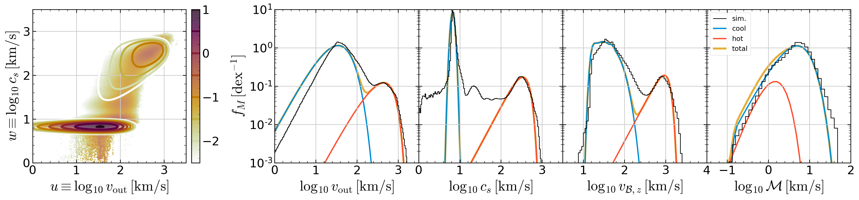
Figure 3: (a) Mass Loading

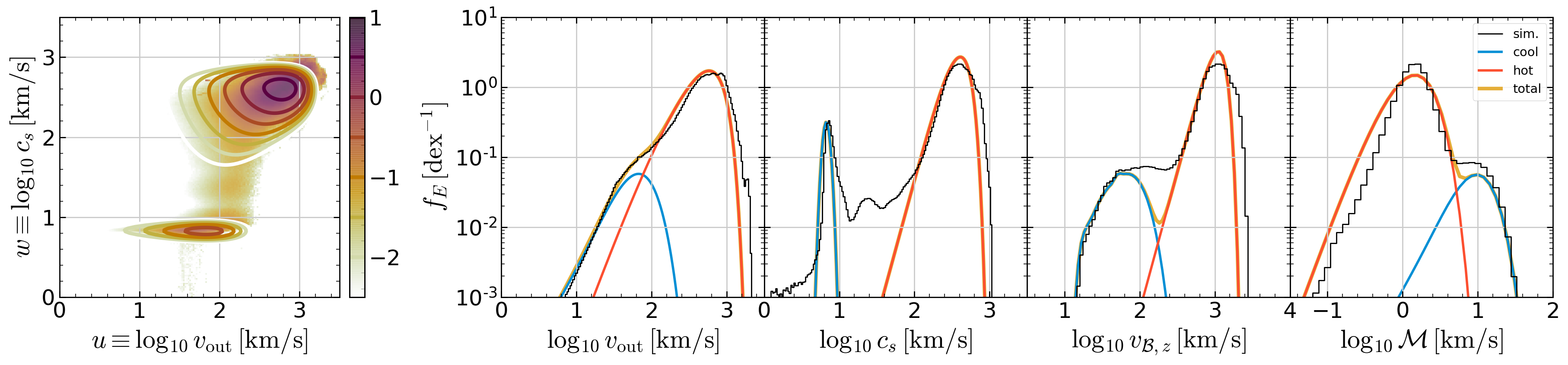
Figure 4: (b) Energy Loading

Figure 5: Comparison between simulated and model PDFs for R4 at $|z|=H$: (a) mass loading and (b) energy loading. In each row, the first column shows full joint PDFs in logarithmic color scale (${\rm log_{\small 10}}\,f_{M,E}\,[\rm dex^{-2}]$) from the simulation (color) and model (contour). The remaining four panels are histograms showing projections onto (from left to right) $v_{\rm out}$, $c_{s}$, $v_{\mathcal{B},z}$, and $\mathcal{M}$ axes. Model PDFs are separated into cool (blue) and hot (orange) components. The sum of the two (yellow) matches simulated PDFs (black lines) well.

Figure 1 and Figure 2 (see also 2020arXiv200616315K) make clear that the cool and hot gas have quite different loading properties, which suggests that for practical applications it will be necessary to treat these components as two different species. To properly treat hot and cool winds on an individual basis, we first define an analytic two-component mass loading PDF model with an easy-to-use functional form that represents the results of the TIGRESS simulations well. We then combine this with the scaling relations for phase-separated loading factors (presented in Table 5 of 2020arXiv200616315K) and our reconstruction method (Equation 19, Equation 21, and Equation 22) to derive energy, momentum, and metal loading PDFs. We emphasize that the objective is not to describe every detail of the PDFs but to reasonably capture the overall behavior over the range of $\Sigma_{\rm SFR}/\,M_{\odot}\,{\rm kpc}^{-2}\,{\rm yr}^{-1}\in(10^{-4},1)$ covered in the simulation suite. With a goal of optimizing both physical fidelity and technical simplicity, we have found that just two free parameters are needed in our wind loading model: $\Sigma_{\rm SFR}$ and $Z_{\rm ISM}$. As we shall show, these two parameters encapsulate the essential aspects of local conditions of star-forming disks needed for characterizing wind properties.

For the cool outflow ($T<2\times 10^{4}\,{\rm K}$), we find that a model combining log-normal and generalized gamma functions,

$$\begin{split}\tilde{f}_{M}^{\rm cool}(u,w)=&A_{c}\left({\frac{v_{\rm out}}{v_{\rm out,0}}}\right)^{2}\exp\left[{-\left({\frac{v_{\rm out}}{v_{\rm out,0}}}\right)}\right]\\ &\exp\left[{-\frac{1}{2}\left({\frac{\ln(c_{s}/c_{\rm s,0})}{\sigma}}\right)^{2}}\right],\end{split}$$ (23)

describes the general shape of the distribution reasonably well. Here, $A_{c}=(\ln 10)^{2}/(2\pi\sigma^{2})^{1/2}=2.12/\sigma$. For this functional form, the mean outflow velocity is $2v_{\rm out,0}$. To fit the simulation PDFs at $|z|=H$, we adopt constant values for $c_{\rm s,0}=6.7\,{\rm km}\,{\rm s}^{-1}$ and $\sigma=0.1$, while $v_{\rm out,0}$ is a function of $\Sigma_{\rm SFR}$:

$$\frac{v_{\rm out,0}}{\,{\rm km}\,{\rm s}^{-1}}=v_{0}\Sigma_{\rm SFR,0}^{0.23}+3$$ (24)

where $v_{0}=25$ and $\Sigma_{\rm SFR,0}\equiv\Sigma_{\rm SFR}/\,M_{\odot}\,{\rm kpc}^{-2}\,{\rm yr}^{-1}$. The adopted form in Equation 24 differs slightly from the linear regression result presented in 2020arXiv200616315K (Eq. 57 there) to (1) adjust for a specific PDF shape adopted here, and (2) avoid arbitrarily low outflow velocity at very low $\Sigma_{\rm SFR}$. We find that only small adjustments are needed in the parameters to describe the simulation PDFs at larger $|z|$: $(v_{0},c_{\rm s,0}/(\,{\rm km}\,{\rm s}^{-1}))=(45,7.5)$, $(45,8.5)$, and $(60,10)$ at $|z|=2H$, 500 pc, and 1 kpc, respectively. This adjustment is physically reasonable because only the higher $v_{\mathcal{B},z}$ components of cool outflows can travel farther.

For the hot outflow ($T>5\times 10^{5}\,{\rm K}$), we construct a model mass PDF using two generalized gamma functions,

$$\begin{split}\tilde{f}_{M}^{\rm hot}(u,w)=&A_{h}\left({\frac{v_{\mathcal{B},z}}{v_{\mathcal{B},0}}}\right)^{2}\exp\left[{-\left({\frac{v_{\mathcal{B},z}}{v_{\mathcal{B},0}}}\right)^{4}}\right]\\ &\left({\frac{\mathcal{M}}{\mathcal{M}_{0}}}\right)^{3}\exp\left[{-\left({\frac{\mathcal{M}}{\mathcal{M}_{0}}}\right)}\right].\end{split}$$ (25)

The arguments $v_{\mathcal{B},z}=(v_{\rm out}^{2}+5c_{s}^{2})^{1/2}$ and Mach number $\mathcal{M}\equiv v_{\rm out}/c_{s}$ can be directly constructed from $u$ and $w$. Here, $A_{h}=(\ln 10)^{2}[2/\sqrt{\pi}]=5.98$. For this functional form, the mean values of $v_{\mathcal{B},z}$ and $\mathcal{M}$ are $0.69v_{\mathcal{B},0}$ and $3\mathcal{M}_{0}$. We adopt a constant value of $\mathcal{M}_{0}=0.5$, and a scaling relation for $v_{\mathcal{B},0}$:

$$\frac{v_{\mathcal{B},0}}{10^{3}\,{\rm km}\,{\rm s}^{-1}}=2.4\frac{\Sigma_{\rm SFR,0}^{1/2}}{2+\Sigma_{\rm SFR,0}^{1/2}}+0.8.$$ (26)

This adopted form is different from the linear regression presented in 2020arXiv200616315K (Eq. 60 there) to (1) keep $v_{\mathcal{B}}\leq v_{\rm ej}$ at high $\Sigma_{\rm SFR}$ and (2) accommodate a flattening at low $\Sigma_{\rm SFR}$. The same hot outflow model works well at all four $|z|$ locations where the simulation PDFs are calculated. Given the generally high specific energy of the hot outflow, the shape of the PDF changes little within the range of $|z|$ we consider. Note that Equation 23 and Equation 25 satisfy $\int\tilde{f}_{M}(u,w)dudw=1$ individually.

As models for the mass loading of the cool and hot phase at $|z|=H$, we adopt power laws

$${\tilde{\eta}_{M}^{\rm{cool}}}=0.85\,\Sigma_{\rm SFR,0}^{-0.44}$$ (27)

$${\tilde{\eta}_{M}^{\rm{hot}}}=0.20\,\Sigma_{\rm SFR,0}^{-0.07}$$ (28)

similar to the relations derived in 2020arXiv200616315K (see Fig. 8a,b there). As we are ignoring the intermediate component, the normalization in ${\tilde{\eta}_{M}^{\rm{hot}}}$ is slightly larger (by a factor 1.4) than that in 2020arXiv200616315K. We also note that ${\tilde{\eta}_{M}}\equiv{\tilde{\eta}_{M}^{\rm{cool}}}+{\tilde{\eta}_{M}^{\rm{hot}}}$ is not identical to the single combined power law fit shown in Fig. 13a of 2020arXiv200616315K. The model mass PDF obtained by combining the cool and hot components is given by

$$\tilde{f}_{M}(u,w)=\frac{{\tilde{\eta}_{M}^{\rm{cool}}}}{{\tilde{\eta}_{M}}}\tilde{f}_{M}^{\rm cool}+\frac{{\tilde{\eta}_{M}^{\rm{hot}}}}{{\tilde{\eta}_{M}}}\tilde{f}_{M}^{\rm hot}$$ (29)

Figure 5 compares the simulated and model joint PDFs of model R4 in the $(u,w)$ plane (first column, color and contour, respectively) and projections along the ${\rm log_{\small 10}}v_{\rm out}$, ${\rm log_{\small 10}}c_{s}$, ${\rm log_{\small 10}}v_{\mathcal{B},z}$, and ${\rm log_{\small 10}}\mathcal{M}$ axes (from second to fifth column). Panels with projected PDFs show the combined model (yellow lines) and the individual cool (blue lines) and hot (red lines) components separately. The combined model PDF follows the original PDF from the simulation (shown as black) reasonably well, modulo a dearth of intermediate temperature gas $w\in(1,2)$ and cold gas $w<0.5$ (but since these have low mass and energy loading factors, this makes no practical difference).

We derive model PDFs for momentum, energy, and metal loading factors as

$$\tilde{f}_{q}=\frac{{\tilde{\eta}_{q}^{\rm{cool}}}}{{\tilde{\eta}_{q}}}\tilde{f}_{q}^{{\rm cool},r}+\frac{{\tilde{\eta}_{q}^{\rm{hot}}}}{{\tilde{\eta}_{q}}}\tilde{f}_{q}^{{\rm hot},r}$$ (30)

where $q=p$, $E$, and $Z$, and $\tilde{f}_{q}^{{\rm ph},r}$ is the reconstructed model PDF for each phase (ph=cool or hot) using Equations (19), (21), and (22). As an example, for momentum

$$\tilde{f}_{p}^{{\rm ph},r}=\frac{\tilde{\eta}_{M}^{{\rm ph}}}{\tilde{\eta}_{p}^{{\rm ph}}}\frac{v_{\rm out}^{2}+c_{s}^{2}}{v_{p}v_{\rm out}}\tilde{f}_{M}^{\rm ph},$$ (31)

with analogous expressions for $\tilde{f}_{E}^{{\rm ph},r}$ and $\tilde{f}_{Z}^{{\rm ph},r}$ based on Equations (21) and (22). As we combine Equation 30 and Equation 31 (or analogous expressions for $q=E$ and $Z$), $\tilde{\eta}_{q}^{\rm ph}$ cancels out, and we only need models for the total momentum, energy, and metal loading factors once we have constructed $\tilde{f}_{M}$ using the phase-separated ${\tilde{\eta}_{M}^{\rm{cool}}}$ and ${\tilde{\eta}_{M}^{\rm{hot}}}$. We combine the power-laws in $\Sigma_{\rm SFR}$ for cool and hot phases at $|z|=H$ from Table 5 of 2020arXiv200616315K to obtain total loading factors:

$${\tilde{\eta}_{p}} =0.04\Sigma_{\rm SFR,0}^{-0.29}+0.1\Sigma_{\rm SFR,0}^{0.02}$$ (32)

$${\tilde{\eta}_{E}} =0.01\Sigma_{\rm SFR,0}^{-0.12}+0.2\Sigma_{\rm SFR,0}^{0.14}$$ (33)

$${\tilde{\eta}_{Z}} =1.5\Sigma_{\rm SFR,0}^{-0.36}+0.42\Sigma_{\rm SFR,0}^{0.04}.$$ (34)

We then renormalize the reconstructed model PDFs to make $\int\tilde{f}_{q}dudw=1$.

Figure 5(b) shows the model energy loading PDF $\tilde{f}_{E}$ in comparison to the simulated energy loading PDF. Again, the agreement between the simulated and model PDFs are good.

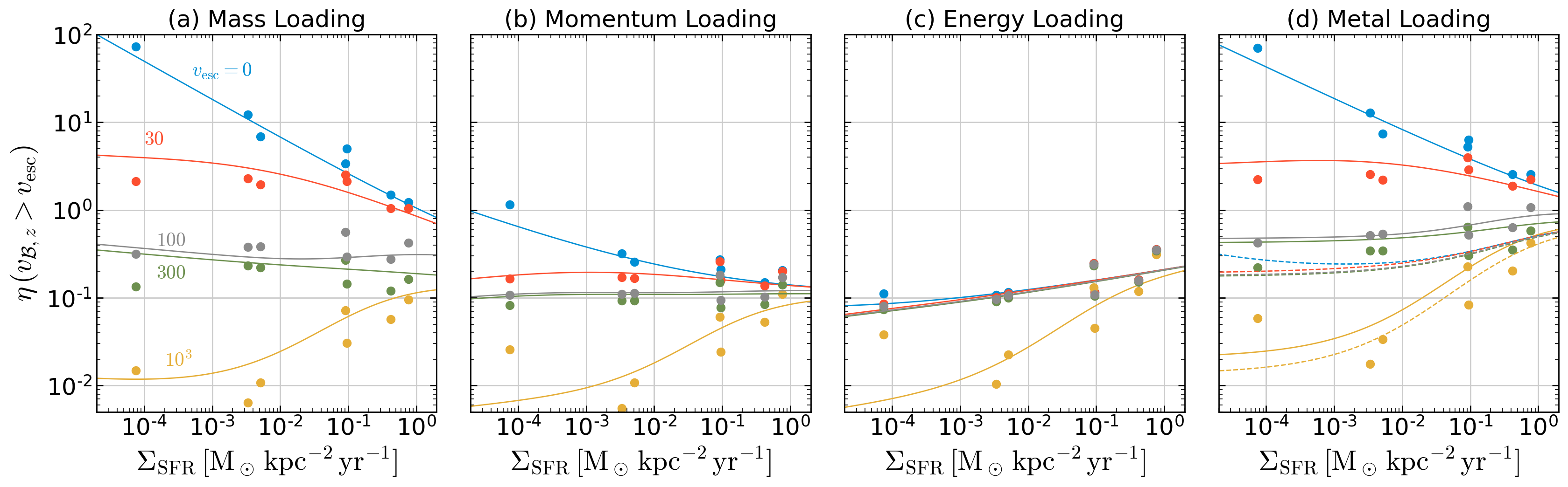
Figure 6: Loading factors for outflows with $v_{\mathcal{B},z}>v_{\rm esc}$ (Equation 35) at $|z|=H$. Filled circles are directly calculated from the simulation PDFs, while solid lines are from the model PDFs. Solid and dashed lines in (d) denote the model loading factors for $Z_{\rm ISM}=0.02$ and 0, respectively. Overall, the model tracks the general behavior of the simulation results.

To check the validity of the model PDFs over a range of $\Sigma_{\rm SFR}$, we compute loading factors for outflows for $v_{\mathcal{B},z}>v_{\rm esc}$,

$$\eta_{q}(v_{\mathcal{B},z}>v_{\rm esc})\equiv\tilde{\eta}_{q}\int_{v_{\mathcal{B},z}=v_{\rm esc}}^{\infty}\tilde{f}_{q}(u,w)dudw,$$ (35)

where $q=M$, $p$, $E$, and $Z$. Figure 6 compares the model $\eta_{q}(v_{\mathcal{B},z}>v_{\rm esc})$ at varying $v_{\rm esc}=0$, 30, 100, 300, and $10^{3}\,{\rm km}\,{\rm s}^{-1}$ to direct results from the simulations at $|z|=H$. These can be thought of as idealized outflow loading properties in halos with varying escape velocities. Direct results from the TIGRESS simulations are shown as filled circles, and the model compares well at all $\Sigma_{\rm SFR}$ and $v_{\rm esc}$.

Note that for the purpose of this test, we normalize the model metal loading PDF for a fixed ISM metallicity, $Z_{\rm ISM}=0.02$. We plot as dashed lines in panel (d) the results for $Z_{\rm ISM}=0$, which is equivalent to the instantaneous SN-origin metal loading factors. This puts a floor on the metal loading.

Despite its simplicity, the model correctly captures key behaviors from the simulations remarkably well. In particular, the high sensitivity of mass loading to $v_{\rm esc}$ (most extreme at low $\Sigma_{\rm SFR}$) and the general insensitivity of energy loading to $v_{\rm esc}$ and $\Sigma_{\rm SFR}$ are notable. The former effect is due to the increase of the mass loading and the decrease of outflow velocities of cool gas at low $\Sigma_{\rm SFR}$, while the latter effect owes to the high outflow velocity and near-constant energy loading of hot gas produced by SNe. More subtle effects, such as the moderate decrease in energy loading at low $\Sigma_{\rm SFR}$ when $v_{\rm esc}>300\,{\rm km}\,{\rm s}^{-1}$, are also reproduced by the model. We note that the energy-loading behavior of the model is mirrored in the metal-loading for $Z_{\rm ISM}=0$ because this is from SN ejecta, while the increase in metal loading at low $v_{\rm esc}$ for $Z_{\rm ISM}=0.02$ is due to metal loss in low-velocity cool-ISM gas.

4 Practical application

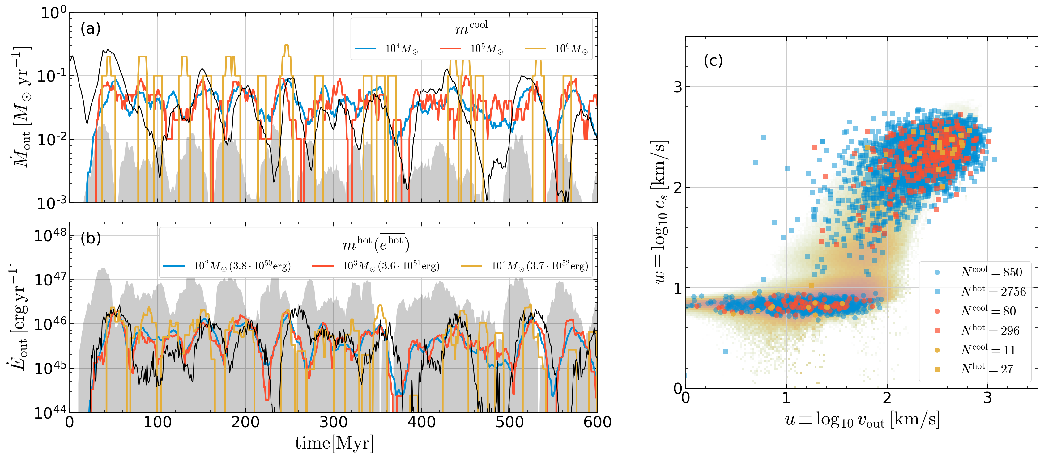
Figure 7: Model sampling demonstration for (a) mass outflow rate of cool gas and (b) energy outflow rate of hot gas at $|z|=H$. The simulation result (black solid) is compared to the model for three different particle mass choices (colored lines; see keys). The input to the model is $\Sigma_{\rm SFR}(t)$ from TIGRESS simulation R8 (representing solar neighborhood conditions with $\Sigma_{\rm gas}\sim 10\,M_{\odot}\,{\rm pc^{-2}}$ and $\Sigma_{\rm SFR}\sim 5\times 10^{-3}\,M_{\odot}\,{\rm kpc}^{-2}\,{\rm yr}^{-1}$), where $\dot{M}_{*}=\Sigma_{\rm SFR}L_{x}L_{y}$ is shown as the grey shaded region in (a) and the corresponding SN energy injection rate is shown as the grey region in (b). (c) Distributions of cool (circles) and hot (squares) outflow particles sampled over $t=220$ - $440\,{\rm Myr}$ from the different mass sampling cases (number of particles drawn is shown in the legend). The simulation PDF at $|z|=H$ over the same time interval is shown in the background.

For practical implementation of our wind launching model, we release a python package Twind with our wind model. As cosmological simulations often launch winds as particles (e.g., 2006MNRAS.373.1265O; 2013MNRAS.436.3031V; but see 2008A&A...477...79D; 2012MNRAS.426..140D; 2014MNRAS.442.3013K for alternative approaches), the package also implements a particle sampling procedure. Twind is based on the two component PDF model at $|z|=H$ described in Section 3, but also supports models at different heights $|z|=2H$, 500 pc, and 1 kpc.

We demonstrate Twind following the procedure outlined in LABEL:sec:appendix_twind using the R8 TIGRESS model, which has the longest simulation duration in our simulation suite. We treat our whole simulation box as equivalent to one resolution element in a cosmological simulation, giving a time series $\dot{M}_{*}=\Sigma_{\rm SFR}L_{x}L_{y}$ where $L_{x}L_{y}=(1024\,{\rm pc})^{2}$ is the horizontal area of the simulation. For this demonstration, we fix $\Delta t=1\,{\rm Myr}$, and adopt constant mass quanta $m^{\rm cool}$ and $m^{\rm hot}$.

Figure 7 shows (a) the mass outflow rate of cool gas from the simulation (black) and the model with three different $m^{\rm cool}$; (b) the energy outflow rate of hot gas from the simulation (black) and the model with three different $m^{\rm hot}$; and (c) the distribution of hot (squares) and cool (circles) particles for the different choices of particle masses. For simplicity, we only show mass (energy) outflow rates of the dominating cool (hot) component (see Figure 5).

As the adopted SFR varies with time, the target mass outflow rate also fluctuates, with median $3.7\times 10^{-2}\,M_{\odot}\,{\rm yr}^{-1}$ and 5(95)th percentile $9.6\times 10^{-3}$ ($6.4\times 10^{-2})\,M_{\odot}\,{\rm yr}^{-1}$. For our chosen $\Delta t=1\,{\rm Myr}$, this translates into outflow mass $\sim 10^{4}-10^{5}\,M_{\odot}$, mostly in cool gas. We thus expect complete, marginal, and incomplete sampling of cool outflows for $m^{\rm cool}=10^{4}\,M_{\odot}$, $10^{5}\,M_{\odot}$, and $10^{6}\,M_{\odot}$, respectively. Figure 7(a) is consistent with this expectation, with good temporal tracking at the lower two masses and poor tracking at the highest mass.

For the R8 simulation, the 5 and 95th percentiles of the energy outflow rate are $4.9\times 10^{44}$ and $1.4\times 10^{46}\,{\rm erg}\,{\rm yr}^{-1}$, corresponding to a range $\sim 5\times 10^{50}-10^{52}\,{\rm erg}$ for $\Delta t=1\,{\rm Myr}$. Given the hot particle mass and model PDF, the mean particle energy is $\overline{e^{\rm hot}}\sim 4\times 10^{50}$ for $m_{\rm hot}=10^{2}\,M_{\odot}$ and increases nearly linearly with the particle mass. Therefore, we expect complete, marginal, and incomplete sampling of hot outflows for $m^{\rm hot}=10^{2}\,M_{\odot}$, $10^{3}\,M_{\odot}$, and $10^{4}\,M_{\odot}$, respectively, as Figure 7(b) demonstrates.

More generally, the necessary resolutions for a fair sampling of mass and energy outflow rates by cool and hot gas, respectively, are

$$m^{\rm cool} \sim\eta_{M}^{\rm cool}\dot{M}_{*}\Delta t$$ (36)

$$\frac{\overline{v_{\mathcal{B},z}}^{2}}{2}m^{\rm hot} \sim\eta_{E}^{\rm hot}E_{\rm SN}\frac{\dot{M}_{*}}{m_{*}}\Delta t,$$ (37)

where $\overline{v_{\mathcal{B},z}}=0.69v_{\mathcal{B},0}$ is the mean Bernoulli velocity of the hot PDF (Equation 25). This implies that the ratio of resolution for hot and cool gas particles should obey

$$\frac{m^{\rm hot}}{m^{\rm cool}}\approx\frac{4E_{\rm SN}}{m_{*}v_{\mathcal{B},0}^{2}}\frac{\eta_{E}^{\rm hot}}{\eta_{M}^{\rm cool}}$$ (38)

which is $\sim 0.01-0.1$ in our simulations (increasing with $\Sigma_{\rm SFR}$). In simulations using particle-based codes, the hot wind particles would therefore generally need to be spawned with smaller mass than the common mass resolution of gas particles.

5 Summary & Outlook

Outflows produced by SN feedback include both hot and cool phases, and even within a single phase there is a range of temperature and flow velocity. Here, we extend the analysis of 2020arXiv200616315K using joint PDFs in sound speed and outflow speed to characterize the mass, momentum, energy, and metal loading of the outflowing gas in a TIGRESS simulation suite, separately treating cool and hot components. We demonstrate that the mass loading PDFs are well described by straightforward analytic expressions (Equation 23 and Equation 25). The momentum, energy, and metal loading PDFs can then be reconstructed from the mass loading PDFs without significant loss of information. A sampling procedure utilizing our two-component PDF, prototyped in python as Twind, is able to successfully reproduce the time-dependent simulated outflow rates in TIGRESS, provided that the respective mass and energy sampling of cool and hot phase outflows are sufficient to follow the true temporal evolution.

The framework developed in this Letter for characterizing multiphase outflows using joint PDFs is quite general, and can be applied to any existing and future simulations in which multiphase outflows naturally emerge. Additional feedback processes including cosmic rays, stellar winds, and radiation as well as additional physics (e.g., thermal conduction) or global geometry may alter the parameters compared to those calibrated using our existing TIGRESS simulation suite. Different functional forms might be needed as well. Regardless of particular details, we consider the formalism we have introduced to analyze simulations and characterize joint PDFs of outflow velocity and sound speed as a fundamental advance in the representation of multiphase outflows.

The joint PDF model and sampling procedure outlined here can be applied to launch multiphase wind particles in cosmological simulations. This would require several changes with respect to current practices in big-box cosmological simulations. First, it is crucial to separately model hot and cool components, rather than a single component. Second, the two components should have separate mass resolution, since resolving energy outflows in the hot gas requires a hot-gas particle mass 1 or 2 orders of magnitude lower than the particle mass required to resolve cool outflows.

In particular, we consider sampling requirements for a solar neighborhood environment with $\Sigma_{\rm SFR}\sim 3\times 10^{-3}\,M_{\odot}\,{\rm kpc}^{-2}\,{\rm yr}^{-1}$, which is typical of star forming disks in both observations (e.g., 2020ApJ...892..148S) and simulations (e.g., 2020arXiv200616314M). The mass resolution for baryons adopted in the Illustris-TNG50 simulations (2019MNRAS.490.3196P; 2019MNRAS.490.3234N) is $\sim 10^{5}\,M_{\odot}$, which would be marginal for realizing mass outflow in cool gas but insufficient for realizing energy (and metal) delivery in hot outflows.

The wind launching model outlined here requires just two parameters, the local ISM metallicity $Z_{\rm ISM}$ and the local star formation rate per unit area in the disk, $\Sigma_{\rm SFR}$. The first is readily available in current cosmological simulation frameworks, but the latter typically is not. There are two different issues. First, the disk scale height is generally not resolved in the current generation of large volume simulations. As a result, the true gas volume density (or pressure) is not known, and without knowledge of the corresponding internal dynamical timescales it is not possible to make a physically-based prediction for the star formation rate on a cell-by-cell basis. To address this issue, either the scale height must be resolved (e.g. in zoom simulations), or a sub-grid model for estimating the true gas scale height must be included. Second, to obtain $\Sigma_{\rm SFR}$ on-the-fly for individual cells, additional computation involving some overhead (e.g., for neighbor searches) would be required.

While the new approach to subgrid wind modeling we describe would involve technical challenges and computational costs, the return on the investment would be wind properties that represent local environments much more faithfully than current approaches. In particular, the usual practice in current cosmological simulations is to scale wind velocities relative to halo virial velocity (e.g., 2016MNRAS.462.3265D; 2019MNRAS.486.2827D; 2018MNRAS.473.4077P), but this does not properly represent the physics of cool gas acceleration, which mostly takes place at small scales within or near the disk in response to the local rate of SN explosions. A wind launching model calibrated based on resolved local simulations would also be predictive and testable through, e.g., global correlations of galaxy properties, which is not the case for empirically-tuned subgrid models.

The results presented here are also of immediate practical use in semi-analytic models (SAMs) of galaxy formation (e.g., 2015MNRAS.453.4337S; 2019MNRAS.487.3581F). In contrast to traditional approaches adopted in SAMs, the inclusion of both mass and energy loading factors enables more sophisticated modeling. For example, many SAMs only account for the mass loss from the ISM due to outflows, and do not include the effects of energy deposited by winds. 2020arXiv200616317P have shown that preventative feedback due to energy deposition from stellar driven winds may be needed to allow SAMs to better reproduce the predictions from the FIRE-2 numerical hydrodynamic simulation suite (2018MNRAS.480..800H), especially in dwarf galaxies. Furthermore, a primary uncertainty in SAMs is what fraction of gas ejected by stellar-driven winds escapes the halo, and on what timescale this ejected gas returns to the halo. The $v_{\rm esc}$ dependent loading factors presented here can be used to determine these quantities, thereby removing several of the free parameters that needed to be empirically calibrated in previous generations of SAMs.

Finally, we emphasize that our model only provides outflow properties at launching, close to the galactic disk ($|z|<1\,{\rm kpc}$). To understand and model the impact of multiphase outflows in the context of galaxy formation and evolution, it is necessary to follow wind interactions with the CGM (which may be inflowing; e.g., 2019ApJ...872...47M; 2020MNRAS.498.3664G). These may or may not be resolved in cosmological simulations, or explicitly modeled in SAMs. It is known from zoom-in simulations that there can be large differences between loading factors near the disk and after the interaction with the CGM (e.g., 2015MNRAS.454.2691M; 2017MNRAS.470.4698A; 2019MNRAS.485.2511T), which implies additional ‘‘post-launch’’ subgrid treatments would be required for lower-resolution large-box simulations. Efforts are underway within the SMAUG collaboration to implement our wind launching model, together with additional treatments for the interaction with the CGM, both in numerical hydrodynamic simulations and in next generation SAMs.

Appendix A A brief summary of models and methods

Table 1: Model Parameters

Model	$\left\langle{\Sigma_{\rm gas}}\right\rangle$	$\rho_{\rm sd}$	$t_{\rm orb}$	$R_{0}$	$\Delta x$	$\left\langle{\Sigma_{\rm SFR}}\right\rangle$
R2	74	1	61	2	2	1.1
R4	30	0.45	110	4	2	1.3×10^-1
R8	11	0.092	220	8	4	5.1×10^-3
R16	2.5	0.005	520	16	8	7.9×10^-5
LGR2	75	0.12	120	2	2	4.9×10^-1
LGR4	38	0.055	200	4	2	9.0×10^-2
LGR8	10	0.012	410	8	4	3.2×10^-3

Note. — (1) model name. (2) gas surface density in $M_{\odot}\,{\rm pc}^{-2}$ averaged over $0.5<t/t_{\rm orb}<1.5$. (3) volume density of stars and dark matter at the midplane in $M_{\odot}\,{\rm pc}^{-3}$. (4) orbit time $t_{\rm orb}\equiv 2\pi/\Omega$ in Myr. (5) galactocentric radius in kpc. (6) spatial resolution of the simulation in pc. For all models, $(N_{x},N_{y},N_{z})=(256,256,1792)$ grid zones are used. (7) SFR surface density in $M_{\odot}\,{\rm kpc}^{-2}\,{\rm yr}^{-1}$ averaged over $0.5<t/t_{\rm orb}<1.5$.