Energy-based error bound of physics-informed
neural network solutions in elasticity

Abstract

An energy-based a posteriori error bound is proposed for the physics-informed neural network solutions of elasticity problems. An admissible displacement-stress solution pair is obtained from a mixed form of physics-informed neural networks, and the proposed error bound is formulated as the constitutive relation error defined by the solution pair. Such an error estimator provides an upper bound of the global error of neural network discretization. The bounding property, as well as the asymptotic behavior of the physics-informed neural network solutions, are studied in a demonstrating example.

Keywords physics-informed neural network  $\cdot$ constitutive relation error  $\cdot$ a posteriori error estimation  $\cdot$ machine learning

1 Introduction

During the past decade, the application of deep neural networks, also known as deep learning, has gained a significant momentum for a variety of tasks including image classification [7, 22], speech recognition [11, 2], autonomous driving [34, 12], and e-commerce [14, 35], to name a few, see [26, 10] for more details. In a recent study, it was shown that neural networks can also be used for the solution and identification of partial differential equations [31, 30]. To that end, the solution space is constructed through deep neural network approximations and the partial derivatives are evaluated using automatic differentiation [5]. A loss function, in the form of a mean-squared error norm (MSE), is constructed to include the differential equations as well as the initial and boundary conditions. Minimization of such a loss function on a sampling grid results in an approximate solution to the problem under study. This approach is now commonly known as physics-informed neural networks (PINNs), and the preliminary studies in [31, 32] have driven a great attention to this approach.

More recently, the methodology of PINNs has been widely applied in the contexts of both forward and inverse problems of fluid mechanics [32, 37, 18, 27], solid mechanics [16, 33], heat transfer [39, 15], flow in porous media [19, 6] and so on. Moreover, the PINNs have also been investigated in their variational or fractional forms [20, 21, 28, 38]. In most of these studies, the PINN methodology is merely used as a tool and adopted to different applications. There is, however, a clear need for fundamental analysis of this methodology and its performance. With the aid of an energy-based a posteriori error bound, we aim to preliminarily investigate the generalization errors and asymptotic behaviors of the PINN solutions of elasticity problems in this work.

To quantify the discretization error in an approximate solution, a posteriori error estimation has been intensively studied for finite element methods [1]. Several families of a posteriori error estimators have been formulated, such as the explicit residual-based error estimator [3], the implicit residual-based error estimator [4], the recovery-based error estimator [40], the hierarchical estimator [8], and the constitutive relation error (CRE) estimator [24]. Among these existing error estimators, the CRE is claimed to provide guaranteed, rigorous, energy-based bounds of the discretization errors in finite element solutions [25, 23]. In this work, we consider a mixed form of PINN approximation for elasticity problems, where the CRE estimation can be naturally employed to formulate an energy-based upper bound of the discretization errors by neural networks. Asymptotic behaviors of the PINN approximation can thus be observed and assessed through the energy-based error bounds given by the CRE.

Following the introduction, a model problem of elasticity and its mix form of PINN solution is introduced in Section 2. An energy-based error bound is formulated for the model problem based on the CRE estimation in Section 3. In Section 4, the proposed error bound is demonstrated by a 2D elasticity problem, and its asymptotic behaviors are discussed. Finally, conclusions drawn in Section 5.

2 Model problem and a physics-informed neural network solution

2.1 Model problem of elasticity

Consider an elastic body whose undeformed configuration $\bm{X}$ is defined in a domain $\Omega\subset\mathbb{R}^{d}$ ($d=1,2,3$) with a Lipschitz boundary $\Gamma=\Gamma_{D}\cup\Gamma_{N}$, where $\Gamma_{D}\neq\emptyset$ is the Dirichlet boundary, $\Gamma_{N}$ is the Neumann boundary, and $\Gamma_{D}\cap\Gamma_{N}=\emptyset$. The elastic body is subjected to a prescribed body force of density $\bm{f}\in[L^{2}(\Omega)]^{d}$ in $\Omega$ with respect to the undeformed volume, a prescribed displacement $\bm{u}_{D}$ on $\Gamma_{D}$, and a prescribed surface force of density $\bm{t}\in[L^{2}(\Gamma_{N})]^{d}$ with respect to the undeformed surface area. An elasticity problem is seek to find the the vector field of displacements $\bm{u}:\Omega\to\mathbb{R}^{d}$ and the stress tensor field $\bm{\sigma}:\Omega\to\mathbb{R}^{d\times d}$ that satisfy (i) the compatibility condition:

$$\bm{u}\in[H_{1}(\Omega)]^{d}\quad\text{and}\quad\bm{u}=\bm{u}_{D}\quad\mathrm{on}\;\Gamma_{D}\,,$$ (1)

i.e. the continuity of the displacement field $\bm{u}$ and the Dirichlet boundary condition; (ii) the equilibrium condition:

$$\mathrm{div}\bm{\sigma}+\bm{f}=\bm{0}\quad\text{and}\quad\mathrm{in}\;\Omega\,,\quad\bm{\sigma}\bm{n}=\bm{t}\quad\mathrm{on}\;\Gamma_{N}\,,$$ (2)

i.e. the momentum equation and the Neumann boundary condition; as well as (iii) the elastic constitutive relation:

$$\bm{\sigma}=\mathcal{C}[\nabla\bm{u}]\,,$$ (3)

in which $\mathcal{C}:\mathbb{R}^{d\times d}\to\mathbb{R}^{d\times d}$ denotes the constitutive relation that maps the displacement gradient $\nabla\bm{u}$ to the stress tensor $\bm{\sigma}$. Note that $\bm{\sigma}$ is taken as the Cauchy stress tensor in linear elasticity under small deformation while more generally considered as the first Piola-Kirchhoff stress tensor in hyperelasticity under finite deformation. The constitutive relation $\mathcal{C}$ can be expressed in the following form in hyperelasticity:

$$\bm{\sigma}=\partial W(\nabla\bm{u})/\partial(\nabla\bm{u})\,,$$ (4)

where $W:\mathbb{R}^{d\times d}\to\mathbb{R}$ is the potential energy density of the considered material. As a special case of hyperelasticity, linear elasticity has the potential energy density in the form of $W=\frac{1}{2}(\nabla\bm{u}):\bm{K}:(\nabla\bm{u})$, $\bm{K}$ being the Hooke’s stiffness tensor, and the constitutive relation is the Hooke’s law $\bm{\sigma}=\bm{K}:\nabla\bm{u}$.

Moreover, for the follow-up discussions on error bounding, the complementary energy density $W^{*}:\mathbb{R}^{d\times d}\to\mathbb{R},{\bf\it\tau}\mapsto W^{*}({\bf\it\tau})$ is introduced as the Legendre transformation of $W$, i.e.,

$$W^{*}({\bf\it\tau})=\sup_{{\bf\it\epsilon}\in\mathbb{R}^{d\times d}}\left\{{\bf\it\tau}:{\bf\it\epsilon}-W({\bf\it\epsilon})\right\}\,.$$ (5)

Assuming that the potential energy density $W$ is a convex function, the constitutive relation (3) can thus be alternatively written as

$$W(\nabla{\bf\it u})+W^{*}({\bf\it\sigma})-{\bf\it\sigma}:\nabla{\bf\it u}=0\,.$$ (6)

2.2 A mixed form of PINN solutions

In this work, we use separate neural networks to approximate the components of both the displacement field ${\bf\it u}$ and the stress field ${\bf\it\sigma}$. Taking the case of $d=2$ as an example, one has

$${\bf\it u}({\bf\it X})\simeq{\bf\it u}^{\texttt{NN}}({\bf\it X})=\begin{bmatrix}u_{x}^{\texttt{NN}}({\bf\it X})\\ u_{y}^{\texttt{NN}}({\bf\it X})\end{bmatrix}\,,\quad{\bf\it\sigma}({\bf\it X})\simeq{\bf\it\sigma}^{\texttt{NN}}({\bf\it X})=\begin{bmatrix}\sigma_{xx}^{\texttt{NN}}({\bf\it X})&\sigma_{xy}^{\texttt{NN}}({\bf\it X})\\ \sigma_{yx}^{\texttt{NN}}({\bf\it X})&\sigma_{yy}^{\texttt{NN}}({\bf\it X})\end{bmatrix}\,.$$ (7)

Note that $\sigma_{xy}=\sigma_{yx}$ for linear elasticity. To train these neural networks informed by the governing equations (1), (2), and (3), a loss function $\mathcal{L}$ can be formulated as

$$\begin{split}\mathcal{L}=&~{}\texttt{MSE}_{\Gamma_{D}}+\texttt{MSE}_{{\bf\it f}}+\texttt{MSE}_{\Gamma_{N}}+\eta\texttt{MSE}_{\mathcal{C}}+\alpha(\texttt{MSE}_{{\bf\it u}}+\texttt{MSE}_{{\bf\it\sigma}})\,,\\ \texttt{MSE}_{\Gamma_{D}}=&~{}\frac{1}{N_{\Gamma_{D}}}\sum_{k=1}^{N_{\Gamma_{D}}}\|{\bf\it u}^{\texttt{NN }}({\bf\it X}_{k}|_{\Gamma_{D}};{\bf\it\theta})-{\bf\it u}_{D}({\bf\it X}_{k}|_{\Gamma_{D}})\|^{2}_{2}\,,\\ \texttt{MSE}_{{\bf\it f}}=&~{}\frac{1}{N_{\Omega}}\sum_{k=1}^{N_{\Omega}}\|\mathrm{div}{\bf\it\sigma}^{\texttt{NN}}({\bf\it X}_{k}|_{\Omega})+{\bf\it f}({\bf\it X}_{k}|_{\Omega})\|_{F}^{2}\,,\\ \texttt{MSE}_{\Gamma_{N}}=&~{}\frac{1}{N_{\Gamma_{N}}}\sum_{k=1}^{N_{\Gamma_{N}}}\|{\bf\it\sigma}^{\texttt{NN}}({\bf\it X}_{k}|_{\Gamma_{N}}){\bf\it n}-{\bf\it t}({\bf\it X}_{k}|_{\Gamma_{N}})\|_{2}^{2}\,,\\ \texttt{MSE}_{\mathcal{C}}=~{}&\frac{1}{N_{\Omega}}\sum_{k=1}^{N_{\Omega}}\|{\bf\it\sigma}^{\texttt{NN}}({\bf\it X}_{k}|_{\Omega})-\mathcal{C}[\nabla{\bf\it u}^{\texttt{NN}}({\bf\it X}_{k}|_{\Omega})]\|_{F}^{2}\,,\\ \texttt{MSE}_{{\bf\it u}}=&~{}\frac{1}{N_{\Omega}}\sum_{k=1}^{N_{\Omega}}\|{\bf\it u}^{\texttt{NN}}({\bf\it X}_{k}|_{\Omega})-{\bf\it u}({\bf\it X}_{k}|_{\Omega})\|_{2}^{2}\,,\\ \texttt{MSE}_{{\bf\it\sigma}}=~{}&\frac{1}{N_{\Omega}}\sum_{k=1}^{N_{\Omega}}\|{\bf\it\sigma}^{\texttt{NN}}({\bf\it X}_{k}|_{\Omega})-{\bf\it\sigma}({\bf\it X}_{k}|_{\Omega})\|_{F}^{2}\,.\end{split}$$ (8)

where $\{{\bf\it X}_{1}|_{\Omega},\cdots,{\bf\it X}_{N_{\Omega}}|_{\Omega}\}$, $\{{\bf\it X}_{1}|_{\Gamma_{N}},\cdots,{\bf\it X}_{N_{\Gamma_{N}}}|_{\Gamma_{N}}\}$ and $\{{\bf\it X}_{1}|_{\Gamma_{D}},\cdots,{\bf\it X}_{N_{\Gamma_{D}}}|_{\Gamma_{D}}\}$ are the collocation points over the domain $\Omega$ and those along the boundaries $\Gamma_{N}$ and $\Gamma_{D}$, respectively. $\eta\in\mathbb{R}^{+}$ is the penalty coefficient for imposing the constitutive relation (3). $\alpha$ is a 0-1 binary variable: the case $\alpha=0$ is a pure boundary value problem (BVP), while the case $\alpha=1$ considers the enhancement by the collocation data of ${\bf\it u}$ and ${\bf\it\sigma}$ over $\Omega$, i.e., the formulation (8) gives a physics-informed regression with the PDE constraints (1), (2) and (3) when $\alpha=1$ .

3 An energy-based error bound

3.1 Constitutive relation error

Definition 3.1 (CRE).

A constitutive relation error (CRE) [25] is a functional $\Psi:KA\times SA\to\mathbb{R}$ defined as follows:

$$\Psi(\hat{{\bf\it u}},\hat{{\bf\it\sigma}})=\int_{\Omega}\left[W(\nabla\hat{{\bf\it u}})+W^{*}(\hat{{\bf\it\sigma}})-\hat{{\bf\it\sigma}}:\nabla\hat{{\bf\it u}}\right]\differential\Omega\,,\quad(\hat{{\bf\it u}},\hat{{\bf\it\sigma}})\in KA\times SA\,,$$ (9)

where $KA=\{\hat{{\bf\it u}}\in[H^{1}(\Omega)]^{d}:\hat{{\bf\it u}}(\Gamma_{D})={\bf\it u}_{D}~{}\text{a.e.}\}$ is the set of all kinematically admissible solutions that satisfy the compatibility condition (1), and $SA=\{\hat{{\bf\it\sigma}}\in[H(\mathrm{div},\Omega)]^{d}:\mathrm{div}\hat{{\bf\it\sigma}}+{\bf\it f}=\mathbf{0}~{}\text{a.e. in }\Omega,~{}\hat{{\bf\it\sigma}}{\bf\it n}={\bf\it t}~{}\text{a.e. on }\Gamma_{N}\}$ is the set of all statically admissible solutions that satisfy the equilibrium condition (2).

A natural result of the Legendre transformation (5) is the Fenchel-Young inequality $W({\bf\it\epsilon})+W^{*}({\bf\it\tau})-{\bf\it\tau}:{\bf\it\epsilon}\geq 0$, $\forall({\bf\it\epsilon},{\bf\it\tau})\in\mathbb{R}^{d\times d}\times\mathbb{R}^{d\times d}$, which further gives the following proposition.

Proposition 3.1.

$\Psi(\hat{{\bf\it u}},\hat{{\bf\it\sigma}})\geq 0$, $\forall(\hat{{\bf\it u}},\hat{{\bf\it\sigma}})\in KA\times SA$.

To evaluate the errors between the admissible fields $(\hat{{\bf\it u}},\hat{{\bf\it\sigma}})\in KA\times SA$ and the exact fields $({\bf\it u},{\bf\it\sigma})$, two error functionals are defined as follows.

Definition 3.2 (Error functionals).

Error functionls $\phi:[H^{1}(\Omega)]^{d}\to\mathbb{R}$ and $\varphi:[H(\mathrm{div},\Omega)]^{d}\to\mathbb{R}$ are introduced in the following form:

$$\begin{split}&\phi({\bf\it e})=\int_{\Omega}\left[W(\nabla({\bf\it u}+{\bf\it e}))-W(\nabla{\bf\it u})-{\bf\it\sigma}:\nabla{\bf\it e}\right]\differential\Omega\,,\quad\bm{e}\in[H^{1}(\Omega)]^{d}\,,\\ &\varphi({\bf\it r})=\int_{\Omega}\left[W^{*}({\bf\it\sigma}+{\bf\it r})-W^{*}({\bf\it\sigma})-{\bf\it r}:\nabla{\bf\it u}\right]\differential\Omega\,,\quad{\bf\it r}\in[H(\mathrm{div},\Omega)]^{d}\,,\end{split}$$ (10)

where $({\bf\it u},{\bf\it\sigma})$ is the exact solution pair of the elasticity problem.

Proposition 3.2.

The error functionals $\phi$ and $\varphi$ have the following properties:

$$\phi(\hat{{\bf\it u}}-{\bf\it u})\geq 0\,,\quad\varphi(\hat{{\bf\it\sigma}}-{\bf\it\sigma})\geq 0\,,\quad\forall(\hat{{\bf\it u}},\hat{{\bf\it\sigma}})\in KA\times SA\,.$$ (11)

Proof. It can be verified that $\phi(\hat{{\bf\it u}}-{\bf\it u})=\Psi(\hat{{\bf\it u}},{\bf\it\sigma})-\Psi({{\bf\it u}},{\bf\it\sigma})=\Psi(\hat{{\bf\it u}},{\bf\it\sigma})$ and $\varphi(\hat{{\bf\it\sigma}}-{\bf\it\sigma})=\Psi({\bf\it u},\hat{{\bf\it\sigma}})-\Psi({\bf\it u},{{\bf\it\sigma}})=\Psi({\bf\it u},\hat{{\bf\it\sigma}})$, both being not less than zero due to Proposition 3.1. The equality holds true if and only if $\hat{{\bf\it u}}={{\bf\it u}}$ and $\hat{{\bf\it\sigma}}={{\bf\it\sigma}}$, respectively.      $\square$

Proposition 3.3.

The CRE and the error functionals in Definition 3.2 are interlinked by the following identity:

$$\Psi(\hat{\bm{u}},\hat{\bm{\sigma}})=\phi(\hat{\bm{u}}-\bm{u})+\varphi(\hat{\bm{\sigma}}-\bm{\sigma})\geq\begin{cases}\phi(\hat{\bm{u}}-\bm{u})\,,\\ \varphi(\hat{\bm{\sigma}}-\bm{\sigma})\,,\end{cases}\quad\forall(\hat{\bm{u}},\hat{\bm{\sigma}})\in KA\times SA\,,$$ (12)

i.e., the CRE can be represented as the sum of two error functionals of the admissible solutions.

Proof. From the definitions of error functionals (10) and that of the CRE (9), one has

$$\begin{split}&~{}\phi(\hat{\bm{u}}-\bm{u})+\varphi(\hat{\bm{\sigma}}-\bm{\sigma})\\ =&~{}\int_{\Omega}\left[\left(W(\nabla\hat{{\bf\it u}})+W^{*}(\hat{{\bf\it\sigma}})\right)-\left(W(\nabla{\bf\it u})+W^{*}({{\bf\it\sigma}})\right)-{\bf\it\sigma}:\nabla(\hat{{\bf\it u}}-{\bf\it u})-(\hat{{\bf\it\sigma}}-{\bf\it\sigma}):\nabla{\bf\it u}\right]\differential\Omega\\ =&~{}\left(\Psi(\hat{\bm{u}},\hat{\bm{P}})+\int_{\Omega}\hat{{\bf\it\sigma}}:\nabla\hat{{\bf\it u}}~{}\differential\Omega\right)-\int_{\Omega}{\bf\it\sigma}:\nabla{\bf\it u}~{}\differential\Omega-\int_{\Omega}\left[{\bf\it\sigma}:\nabla(\hat{{\bf\it u}}-{\bf\it u})+(\hat{{\bf\it\sigma}}-{\bf\it\sigma}):\nabla{\bf\it u}\right]~{}\differential\Omega\\ =&~{}\Psi(\hat{\bm{u}},\hat{\bm{P}})+\int_{\Omega}(\hat{{\bf\it\sigma}}-{\bf\it\sigma}):\nabla(\hat{{\bf\it u}}-{\bf\it u})~{}\differential\Omega\,.\end{split}$$

Green’s formula gives that

$$\int_{\Omega}\bm{\tau}:\nabla\bm{v}~{}\differential\Omega=\int_{\Omega}-\mathrm{div}\bm{\tau}\cdot\bm{v}\differential{\Omega}+\int_{\Gamma}(\bm{\tau}\bm{n})\cdot\bm{v}\differential{\Gamma}\,,\quad(\bm{v},\bm{\tau})\in[H_{1}(\Omega)]^{d}\times[H(\mathrm{div},\Omega)]^{d}\,.$$ (13)

Taking ${\bf\it\tau}=\hat{{\bf\it\sigma}}-{\bf\it\sigma}$ and ${\bf\it v}=\hat{{\bf\it u}}-{\bf\it u}$ yields that $\int_{\Omega}(\hat{{\bf\it\sigma}}-{\bf\it\sigma}):\nabla(\hat{{\bf\it u}}-{\bf\it u})~{}\differential\Omega=0$, since $\mathrm{div}(\hat{{\bf\it\sigma}}-{\bf\it\sigma})=\mathbf{0}$ in $\Omega$, $(\hat{{\bf\it\sigma}}-{\bf\it\sigma}){\bf\it n}=\mathbf{0}$ on $\Gamma_{N}$, and $\hat{{\bf\it u}}-{\bf\it u}=\mathbf{0}$ on $\Gamma_{D}$. Then (12) is obtained in view of the fact that $\phi(\hat{\bm{u}}-\bm{u})\geq 0$ and $\varphi(\hat{\bm{\sigma}}-\bm{\sigma})\geq 0$.      $\square$

In linear elasticity under small deformation, the difference between deformed and undeformed configurations is not taken into consideration, and the first Piola-Kirchhoff stress tensor coincides with the Cauchy stress tensor. The potential and complementary energy densities are written as $W(\nabla{\bf\it u})=\frac{1}{2}\nabla{\bf\it u}:{\bf\it K}:\nabla{\bf\it u}$ and $W^{*}({\bf\it\sigma})=\frac{1}{2}{\bf\it\sigma}:{\bf\it K}^{-1}:{\bf\it\sigma}$, respectively. The error functionals for both the displacement and stress fields are formulated as $\phi({\bf\it e})=\int_{\Omega}\frac{1}{2}\nabla{\bf\it e}:{\bf\it K}:\nabla{\bf\it e}~{}\differential\Omega$ and $\varphi({\bf\it r})=\int_{\Omega}\frac{1}{2}{\bf\it r}:{\bf\it K}^{-1}:{\bf\it r}~{}\differential\Omega$, respectively, $({\bf\it e},{\bf\it r})\in(KA-{\bf\it u})\times(SA-{\bf\it\sigma})$. Furthermore, the CRE has a second-order form $\Psi(\hat{\bm{u}},\hat{\bm{\sigma}})=\int_{\Omega}\frac{1}{2}(\hat{{\bf\it\sigma}}-{\bf\it K}:\nabla\hat{{\bf\it u}}):{\bf\it K}^{-1}:(\hat{{\bf\it\sigma}}-{\bf\it K}:\nabla\hat{{\bf\it u}})~{}\differential\Omega$, $(\hat{{\bf\it u}},\hat{{\bf\it\sigma}})\in KA\times SA$. Moreover, we refer to [13] for a more generalized discussion on CREs in convex problems.

3.2 Bounding global errors in PINN solutions

When $\eta$ is set to be a small value, i.e., $\eta\ll 1$, the compatibility constraint (1) and the equilibrium condition (2) are enforced on ${\bf\it u}^{\texttt{NN}}$ and ${\bf\it\sigma}^{\texttt{NN}}$, respectively, in the sense of minimizing the corresponding penalty terms in $\mathcal{L}$. By taking $\hat{{\bf\it u}}\simeq{\bf\it u}^{\texttt{NN}}$ and $\hat{{\bf\it\sigma}}\simeq{\bf\it\sigma}^{\texttt{NN}}$, the CRE $\Psi$ provides an error bound for both ${\bf\it u}^{\texttt{NN}}$ and ${\bf\it\sigma}^{\texttt{NN}}$, i.e.,

$$\phi({\bf\it u}^{\texttt{NN}}-{\bf\it u})\lesssim\Psi({\bf\it u}^{\texttt{NN}},{\bf\it\sigma}^{\texttt{NN}}),\quad\text{and}\quad\varphi({\bf\it\sigma}^{\texttt{NN}}-{\bf\it\sigma})\lesssim\Psi({\bf\it u}^{\texttt{NN}},{\bf\it\sigma}^{\texttt{NN}})\,,$$ (14)

where the global discretization errors in the neural network solutions ${\bf\it u}^{\texttt{NN}}$ and ${\bf\it\sigma}^{\texttt{NN}}$ are measured by the functionals $\phi$ and $\varphi$, respectively. From the perspective of neural network training, $\phi$ and $\varphi$ are adopted to quantify the global generalization errors in networks ${\bf\it u}^{\texttt{NN}}$ and ${\bf\it\sigma}^{\texttt{NN}}$, respectively. As the solutions $({\bf\it u}^{\texttt{NN}},{\bf\it\sigma}^{\texttt{NN}})$ obtained by minimizing the loss function $\mathcal{L}$ only approximately satisfy the compatibility constraint (1) and the equilibrium condition (2), we use the symbol $\lesssim$ for the bounding property (14) in an approximate sense.

In the CRE estimation for the displacement-based, conforming finite element method, it is required to make additional efforts to construct a stress field that satisfies the equilibrium equation (2). Such stress recovery techniques [25, 29, 9] are usually based on element-wise construction and implemented at a high computational price. However, the mixed form of PINNs gives the admissible solution pair $({\bf\it u}^{\texttt{NN}},{\bf\it\sigma}^{\texttt{NN}})$ simultaneously, then the CRE can be directly applied without additional computational efforts. When a larger amount of training data or a more sophisticated neural network architecture is adopted, the accuracy of ${\bf\it u}^{\texttt{NN}}$ and ${\bf\it\sigma}^{\texttt{NN}}$ can be improved simultaneously through minimizing the loss function $\mathcal{L}$ in (8), and such asymptotic behavior can be indicated by the decay of the CRE value $\Psi$ in the meantime.

4 Numerical example

To demonstrate the proposed error bounds, we consider a square plate defined in the domain $\Omega=]0,1[^{2}$ with unit side length $L_{x}=L_{y}=1$, introduced in [17]. Let us identify different sides of the square with $\Gamma_{x^{-}}=\{{\bf\it X}=(x,y)^{\text{T}}|x=0,y\in[0,1]\}$, $\Gamma_{x^{+}}=\{{\bf\it X}=(x,y)^{\text{T}}|x=1,y\in[0,1]\}$, $\Gamma_{y^{-}}=\{{\bf\it X}=(x,y)^{\text{T}}|y=0,x\in[0,1]\}$, and $\Gamma_{y^{+}}=\{{\bf\it X}=(x,y)^{\text{T}}|y=1,x\in[0,1]\}$. The plate is subjected to the following boundary conditions: (a) $\sigma_{xx}=0$ and $u_{y}=0$ on $\Gamma_{x}^{-}$ and $\Gamma_{x}^{+}$, (b) $u_{x}=u_{y}=0$ on $\Gamma_{y}^{-}$, and (c) $u_{x}=0$ and $\sigma_{yy}=(\lambda+2\mu)Q\sin(\pi x)$ on $\Gamma_{y}^{+}$. Additionally, the plate is subjected to the following body forces:

$$\begin{split}f_{x}(x,y)=&\lambda\left[4\pi^{2}\cos(2\pi x)\sin(\pi y)-\pi\cos(\pi x)Qy^{3}\right]\\ &+\mu\left[9\pi^{2}\cos(2\pi x)\sin(\pi y)-\pi\cos(\pi x)Qy^{3}\right],\\ f_{y}(x,y)=&\lambda\left[-3\sin(\pi x)Qy^{2}+2\pi^{2}\sin(2\pi x)\cos(\pi y)\right]\\ &+\mu\left[-6\sin(\pi x)Qy^{2}+2\pi^{2}\sin(2\pi x)\cos(\pi y)+\pi^{2}\sin(\pi x)Qy^{4}/4\right].\end{split}$$

Here $\lambda$ and $\mu$ are the two Lamé parameters of a homogeneous and isotropic material, and we take $Q=4$. The analytical solution to this problem is given as

$$u_{x}(x,y)=\cos(2\pi x)\sin(\pi y)\quad\text{and}\quad u_{y}(x,y)=\sin(\pi x)Qy^{4}/4$$ (15)

and plotted in Fig. 1.

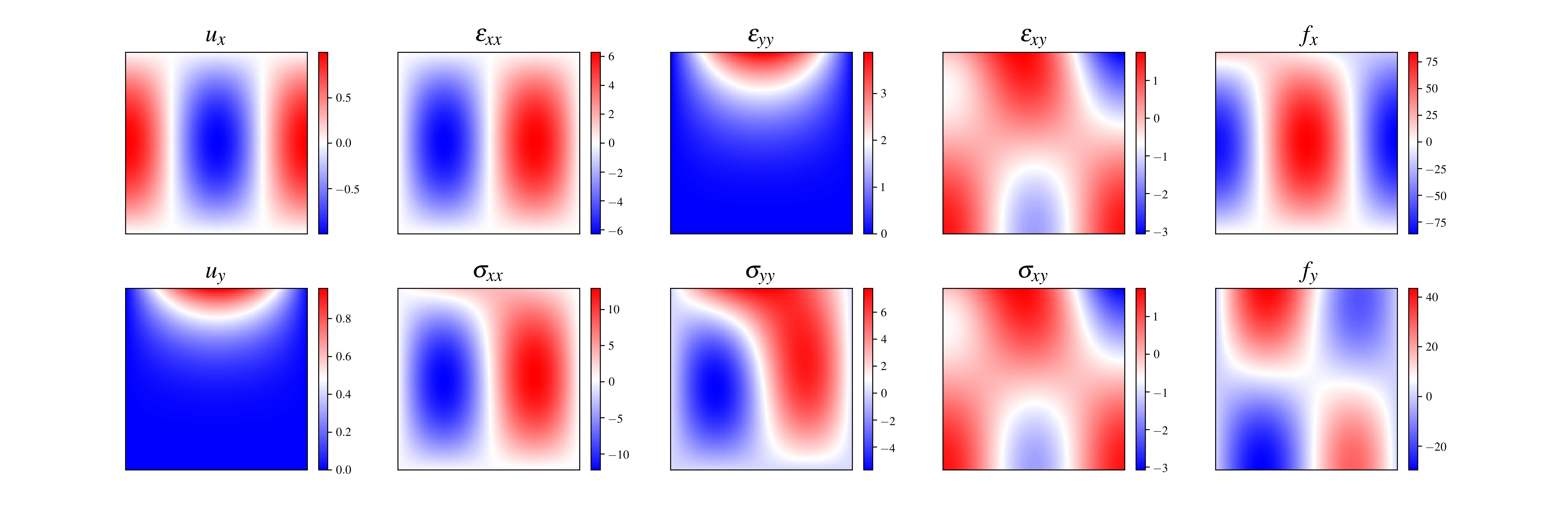
Figure 1: The exact displacement components $(u_{x},u_{y})$, strain components $(\varepsilon_{xx},\varepsilon_{yy},\varepsilon_{xy})$, and stress components $(\sigma_{xx},\sigma_{yy},\sigma_{xy})$ for the linear elasticity problem, subjected to the body forces $(f_{x},f_{y})$.

In this example, the PINN framework is employed in the following two scenarios:

• scenario (a): PINN as a solution method, i.e., $\alpha=0$. The problem is considered as a boundary value problem, where data are given at the boundaries in the form of displacement or stress conditions. A sampling grid of $100\times 100$ is used for the collocation of equilibrium equations and constitutive relations, except when we change the sampling grid to investigate the corresponding asymptotic behaviors. Moreover, we take $\eta=0.01$ in this scenario.

• scenario (b): PINN as a regression method, i.e., $\alpha=1$. It is assumed that the displacement and stress data are given at uniformly distributed grid points, and the objective is to construct a regression model that also satisfies the underlying physics of linear elasticity. Here the data are given on a uniform grid of $40\times 40$, except when we change the sampling grid to investigate the corresponding asymptotic behaviors. Since the grid data for both displacements and stresses already impose very strong constraints on the solution fields, we take $\eta=0$ in this scenario, i.e., loosing the constraints by constitutive relations.

There are three types of errors associated with the training of neural networks, including the optimization error, the generalization error, and the approximation error, as discussed in [36]. Here, we quantify the global generalization errors in the displacement and stress fields by $\phi({\bf\it u}^{\texttt{NN}}-{\bf\it u})$ and $\varphi({\bf\it\sigma}^{\texttt{NN}}-{\bf\it\sigma})$, respectively. All these integrals are approximately evaluated on a fine test grid of $200\times 200$. We consider the following three cases:

• Generalization error in sampling. As the first case, we quantify the generalization errors in the displacement and stress fields with respect to the number of sampling (collocation) points used for optimizing the loss function. Here, we adopt a fixed size neural network with 4 hidden layers and 20 neurons in each layer to construct all the approximate solutions $u_{x}^{\texttt{NN}}$, $u_{y}^{\texttt{NN}}$, $\sigma_{xx}^{\texttt{NN}}$, $\sigma_{yy}^{\texttt{NN}}$, and $\sigma_{xy}^{\texttt{NN}}$. We then use seven grids of sizes $40\times 40$, $50\times 50$, $60\times 60$, $70\times 70$, $80\times 80$, $90\times 90$, and $100\times 100$ to sample the loss function during the optimization and train the neural networks.

• Generalization error in neurons. As the second case, we study the generalization errors in the displacement and stress solutions with respect to the number of neurons per each layer. For this purpose, we fix the number of hidden layers of each network to 4 and change the width of the network as 20, 30, 40, 50, 60, 70, and 80.

• Generalization error in layers. As the last case, we study the generalization errors in the displacement and stress solutions with respect to the number of hidden layers. Therefore, we adopt a fixed number of neurons for each hidden layer as 20 and vary the number of hidden layers from 2 to 10 in scenario (a), while 4 to 10 in scenario (b).

The comparisons of global discretization errors $\phi({\bf\it u}^{\texttt{NN}}-{\bf\it u})$, $\varphi({\bf\it\sigma}^{\texttt{NN}}-{\bf\it\sigma})$ and the CRE $\Psi({\bf\it u}^{\texttt{NN}},{\bf\it\sigma}^{\texttt{NN}})$ are shown in Figs. 2 and 3 for the scenarios (a) and (b), respectively. All results are compiled on a test grid of size $200\times 200$, with which the integrals are approximately calculated. Note that this distinguishes from the classical finite element method in which the results are analyzed at the same locations as they are evaluated, i.e., at the nodes or quadrature points. In all the cases considered in this example, it is verified that the CRE guarantees an upper bound of the global generalization errors in both the displacement and stress solutions by PINNs. As seen in the stacked plots, the equality $\phi({\bf\it u}^{\texttt{NN}}-{\bf\it u})+\varphi({\bf\it\sigma}^{\texttt{NN}}-{\bf\it\sigma})=\Psi({\bf\it u}^{\texttt{NN}},{\bf\it\sigma}^{\texttt{NN}})$ is often not strictly satisfied and there exists a relative error within $15\%$. The reason mainly lies in the fact that the solution fields $({\bf\it u}^{\texttt{NN}},{\bf\it\sigma}^{\texttt{NN}})$ obtained by minimizing $\mathcal{L}$ cannot strictly satisfy the corresponding admissible conditions, thus the term $\int_{\Omega}({\bf\it\sigma}^{\texttt{NN}}-{\bf\it\sigma}):\nabla({\bf\it u}^{\texttt{NN}}-{\bf\it u})~{}\differential\Omega$ cannot vanish (see the proof of Proposition 3.3). In spite of this, the CRE still effectively provides an upper bound of the global discretization errors and can be used as an indicator for the credibility of PINN solutions.

In general, scenario (a) can be considered as an unsupervised learning approach, in which no training data is provided inside the domain, while scenario (b) is of the supervised learning class. The supervised learning method is well understood. With more training points, one can improve the accuracy of the predictions up to a limit depending on the network size. This is indeed what we can observe in the scenario (b), see Fig. 3(b). The use of more training points reduces the generalization errors of the PINN model, and high accuracy can be achieved with very fine training grids. The width and depth of the network also show more predictable behaviour as a result of supervised learning, as shown in Figs. 3(d) and 3(f). On the other hand, without imposing any data inside the domain, solving a PDE problem only by minimizing a loss function that incorporates the governing equations is an unsupervised learning task. This task is generally much harder and requires much more training time and iterations. We find that after a relatively small number of sampling points, the accuracy of predictions by a fixed network architecture can hardly be improved by adding more training points, see Fig. 2(b). Further improvements demand a significant fine-tuning of the optimizer and many training epochs, which we try to avoid here. Such a behavior of PINN as a BVP solution method is also consistent with the observations made in other studies [36]. In this case, the bounding property of the proposed CRE estimator is still guaranteed. Since the true errors are not computable, the CRE estimator can be evaluated for the observation of convergence behavior.

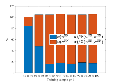
(a) $\phi/\Psi$ and $\varphi/\Psi$ versus training sample grid

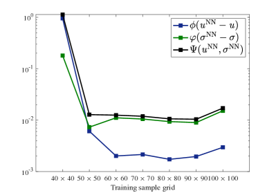
(b) Global generalization errors and CRE versus training sample grid

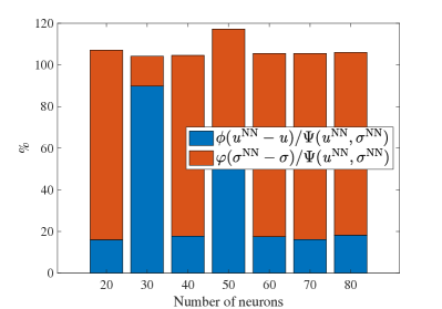
(c) $\phi/\Psi$ and $\varphi/\Psi$ versus number of neurons

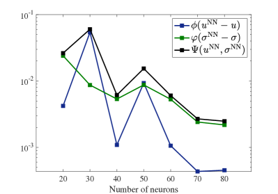
(d) Global generalization errors and CRE versus number of neurons

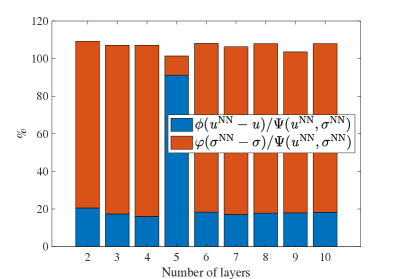
(e) $\phi/\Psi$ and $\varphi/\Psi$ versus number of layers

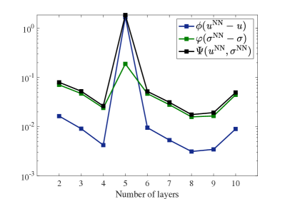
(f) Global generalization errors and CRE versus number of layers

Figure 2: Comparison of the energy error in displacements $\phi({\bf\it u}^{\texttt{NN}}-{\bf\it u})$, the energy error in stresses $\varphi({\bf\it\sigma}^{\texttt{NN}}-{\bf\it\sigma})$, and the CRE $\Psi({\bf\it u}^{\texttt{NN}},{\bf\it\sigma}^{\texttt{NN}})$ in the scenario (a) where PINN is used as a BVP solution method.

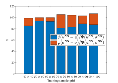
(a) $\phi/\Psi$ and $\varphi/\Psi$ versus training sample grid

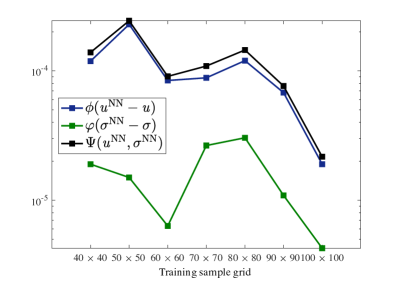
(b) Global generalization errors and CRE versus training sample grid

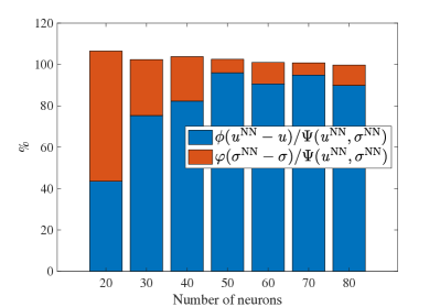
(c) $\phi/\Psi$ and $\varphi/\Psi$ versus number of neurons

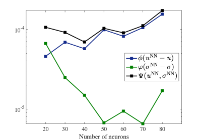
(d) Global generalization errors and CRE versus number of neurons

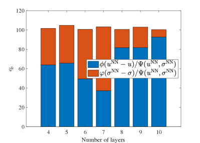
(e) $\phi/\Psi$ and $\varphi/\Psi$ versus number of layers

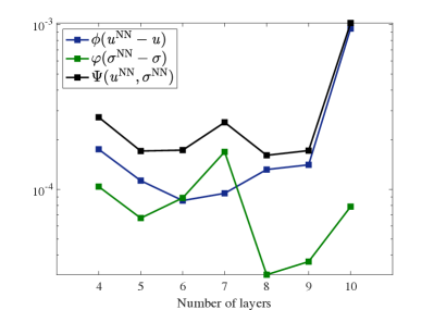
(f) Global generalization errors and CRE versus number of layers

Figure 3: Comparison of the energy error in displacements $\phi({\bf\it u}^{\texttt{NN}}-{\bf\it u})$, the energy error in stresses $\varphi({\bf\it\sigma}^{\texttt{NN}}-{\bf\it\sigma})$, and the CRE $\Psi({\bf\it u}^{\texttt{NN}},{\bf\it\sigma}^{\texttt{NN}})$ in the scenario (b) where PINN is used as a regression method.

5 Conclusions

In this note, we have briefly presented a preliminary work on a posteriori error analysis for the PINN solutions of elasticity problems. An energy-based error bound, defined as a constitutive relation error, is employed to provide an upper bound of the global discretization errors in both the displacements and the stresses solved through a mix form of PINNs. The generalization performance of PINNs is thus assessed by the proposed error bound. In the numerical demonstration, a reference 2D linear elasticity problem is analyzed using PINNs as a forward solver and as a regression tool. Considering a wide range of network hyper parameters, i.e., number of neurons and hidden layers, and number of sampling points, it has been verified that the proposed error bound guarantees an upper bound of the energy-based measures of generalization errors and offers good robustness. The constitutive relation error bound is also directly applicable for hyperelasticity problems, and can be used for goal-oriented error estimation in cooperation with an adjoint problem.

References

- [1] M. Ainsworth and J. T. Oden. A posteriori error estimation in finite element analysis, volume 37. John Wiley & Sons, 2011.
- [2] D. Amodei, S. Ananthanarayanan, R. Anubhai, J. Bai, E. Battenberg, C. Case, J. Casper, B. Catanzaro, Q. Cheng, G. Chen, et al. Deep speech 2: End-to-end speech recognition in english and mandarin. In International conference on machine learning, pages 173–182, 2016.
- [3] I. Babuška and W. C. Rheinboldt. A-posteriori error estimates for the finite element method. International Journal for Numerical Methods in Engineering, 12(10):1597–1615, 1978.
- [4] R. E. Bank and A. Weiser. Some a posteriori error estimators for elliptic partial differential equations. Mathematics of Computation, 44(170):283–301, 1985.
- [5] A. G. Baydin, B. A. Pearlmutter, A. A. Radul, and J. M. Siskind. Automatic differentiation in machine learning: a survey. The Journal of Machine Learning Research, 18(1):5595–5637, 2017.
- [6] Y. W. Bekele. Deep learning for one-dimensional consolidation. arXiv:2004.11689, 2020.
- [7] J. Deng, W. Dong, R. Socher, L.-J. Li, K. Li, and L. Fei-Fei. Imagenet: A large-scale hierarchical image database. In 2009 IEEE conference on computer vision and pattern recognition, pages 248–255. Ieee, 2009.
- [8] P. Deuflhard, P. Leinen, and H. Yserentant. Concepts of an adaptive hierarchical finite element code. IMPACT of Computing in Science and Engineering, 1(1):3–35, 1989.
- [9] L. Gallimard. A constitutive relation error estimator based on traction-free recovery of the equilibrated stress. International Journal for Numerical Methods in Engineering, 78(4):460–482, 2009.
- [10] I. Goodfellow, Y. Bengio, A. Courville, and Y. Bengio. Deep learning, volume 1. MIT press Cambridge, 2016.
- [11] A. Graves, A.-r. Mohamed, and G. Hinton. Speech recognition with deep recurrent neural networks. In 2013 IEEE international conference on acoustics, speech and signal processing, pages 6645–6649. IEEE, 2013.
- [12] S. Grigorescu, B. Trasnea, T. Cocias, and G. Macesanu. A survey of deep learning techniques for autonomous driving. Journal of Field Robotics, 37(3):362–386, 2020.
- [13] M. Guo, W. Han, and H. Zhong. Legendre-fenchel duality and a generalized constitutive relation error. arXiv:1611.05589, 2016.
- [14] J.-W. Ha, H. Pyo, and J. Kim. Large-scale item categorization in e-commerce using multiple recurrent neural networks. In Proceedings of the 22nd ACM SIGKDD International Conference on Knowledge Discovery and Data Mining, pages 107–115, 2016.
- [15] E. Haghighat and R. Juanes. Sciann: A keras wrapper for scientific computations and physics-informed deep learning using artificial neural networks. arXiv:2005.08803, 2020.
- [16] E. Haghighat, M. Raissi, A. Moure, H. Gomez, and R. Juanes. A deep learning framework for solution and discovery in solid mechanics. arXiv:2003.02751, 2020.
- [17] E. Haghighat, M. Raissi, A. Moure, H. Gomez, and R. Juanes. A deep learning framework for solution and discovery in solid mechanics. arXiv:2003.02751, 2020.
- [18] X. Jin, S. Cai, H. Li, and G. E. Karniadakis. Nsfnets (navier-stokes flow nets): Physics-informed neural networks for the incompressible navier-stokes equations. arXiv:2003.06496, 2020.
- [19] T. Kadeethum, T. M. Jørgensen, and H. M. Nick. Physics-informed neural networks for solving nonlinear diffusivity and biot’s equations. PloS one, 15(5):e0232683, 2020.
- [20] E. Kharazmi, Z. Zhang, and G. E. Karniadakis. Variational physics-informed neural networks for solving partial differential equations. arXiv:1912.00873, 2019.
- [21] E. Kharazmi, Z. Zhang, and G. E. Karniadakis. hp-vpinns: Variational physics-informed neural networks with domain decomposition. arXiv:2003.05385, 2020.
- [22] A. Krizhevsky, I. Sutskever, and G. E. Hinton. Imagenet classification with deep convolutional neural networks. In Advances in neural information processing systems, pages 1097–1105, 2012.
- [23] P. Ladevèze and L. Chamoin. The constitutive relation error method: A general verification tool. In Verifying Calculations-Forty Years On, pages 59–94. Springer, 2016.
- [24] P. Ladevèze and D. Leguillon. Error estimate procedure in the finite element method and applications. SIAM Journal on Numerical Analysis, 20(3):485–509, 1983.
- [25] P. Ladevèze and J. P. Pelle. Mastering calculations in linear and nonlinear mechanics. Springer, 2005.
- [26] Y. LeCun, Y. Bengio, and G. Hinton. Deep learning. nature, 521(7553):436–444, 2015.
- [27] Z. Mao, A. D. Jagtap, and G. E. Karniadakis. Physics-informed neural networks for high-speed flows. Computer Methods in Applied Mechanics and Engineering, 360:112789, 2020.
- [28] G. Pang, L. Lu, and G. E. Karniadakis. fpinns: Fractional physics-informed neural networks. SIAM Journal on Scientific Computing, 41(4):A2603–A2626, 2019.
- [29] F. Pled, L. Chamoin, and P. Ladevèze. On the techniques for constructing admissible stress fields in model verification: Performances on engineering examples. International Journal for Numerical Methods in Engineering, 88(5):409–441, 2011.
- [30] M. Raissi and G. E. Karniadakis. Hidden physics models: Machine learning of nonlinear partial differential equations. Journal of Computational Physics, 357:125–141, 2018.
- [31] M. Raissi, P. Perdikaris, and G. E. Karniadakis. Physics-informed neural networks: A deep learning framework for solving forward and inverse problems involving nonlinear partial differential equations. Journal of Computational Physics, 378:686–707, 2019.
- [32] M. Raissi, A. Yazdani, and G. E. Karniadakis. Hidden fluid mechanics: Learning velocity and pressure fields from flow visualizations. Science, 367(6481):1026–1030, 2020.
- [33] C. Rao, H. Sun, and Y. Liu. Physics informed deep learning for computational elastodynamics without labeled data. arXiv:2006.08472, 2020.
- [34] A. E. Sallab, M. Abdou, E. Perot, and S. Yogamani. Deep reinforcement learning framework for autonomous driving. Electronic Imaging, 2017(19):70–76, 2017.
- [35] D. Shankar, S. Narumanchi, H. Ananya, P. Kompalli, and K. Chaudhury. Deep learning based large scale visual recommendation and search for e-commerce. arXiv:1703.02344, 2017.
- [36] Y. Shin, J. Darbon, and G. E. Karniadakis. On the convergence and generalization of physics informed neural networks. arXiv:2004.01806, 2020.
- [37] X. Yang, S. Zafar, J.-X. Wang, and H. Xiao. Predictive large-eddy-simulation wall modeling via physics-informed neural networks. Physical Review Fluids, 4(3):034602, 2019.
- [38] Y. Yang and P. Perdikaris. Physics-informed deep generative models. arXiv:1812.03511, 2018.
- [39] X. Zhao, K. Shirvan, R. K. Salko, and F. Guo. On the prediction of critical heat flux using a physics-informed machine learning-aided framework. Applied Thermal Engineering, 164:114540, 2020.
- [40] O. C. Zienkiewicz and J. Z. Zhu. A simple error estimator and adaptive procedure for practical engineerng analysis. International Journal for Numerical Methods in Engineering, 24(2):337–357, 1987.