Large fluctuations and transport properties of the Lévy-Lorentz gas

Abstract

The Lévy-Lorentz gas describes the motion of a particle on the real line in the presence of a random array of scattering points, whose distances between neighboring points are heavy-tailed i.i.d. random variables with finite mean. The motion is a continuous-time, constant-speed interpolation of the simple symmetric random walk on the marked points. In this paper we study the large fluctuations of the continuous-time process and the resulting transport properties of the model, both annealed and quenched, confirming and extending previous work by physicists that pertain to the annealed framework. Specifically, focusing on the particle displacement, and under the assumption that the tail distribution of the interdistances between scatterers is regularly varying at infinity, we prove a precise large deviation principle for the annealed fluctuations and present the asymptotics of annealed moments, demonstrating annealed superdiffusion. Then, we provide an upper large deviation estimate for the quenched fluctuations and the asymptotics of quenched moments, showing that the asymptotic diffusive regime conditional on a typical arrangement of the scatterers is normal diffusion, and not superdiffusion. Although the Lévy-Lorentz gas seems to be accepted as a model for anomalous diffusion, our findings suggest that superdiffusion is a transient behavior which develops into normal diffusion on long timescales, and raise a new question about how the transition from the quenched normal diffusion to the annealed superdiffusion occurs.

Abstract

[language=french] Le gaz de Lévy-Lorentz modélise le déplacement d’une particule sur l’axe des réels en présence d’obstacles distribués de telle façon que les distances les uns avec les autres sont des variables aléatoires i.i.d. à queue lourde et moyenne finie. La dynamique est donnée par l’interpolation, en temps continu et vitesse fixe, de la marche aléatoire symétrique sur les obstacles. Cet article étudie les grandes fluctuations du processus en temps continu et les propriétés de transport du modèle sous-jacent. Les résultats obtenus dans les cas de désordre “annealed” et “quenched” confirment et généralisent des résultats precedents issus de la physique dans le cas “annealed”. En particulier, sous l’hypothèse que la queue de la loi des distances inter-obstacles est à variation régulière à l’infini, nous prouvons dans le cas “annealed” un principe de grandes déviations et obtenons l’expression asymptotique des moments, qui montrent l’existence d’un regime de sur-diffusion. Dans le cas quenched, nous obtenons l’expression asymptotique des moments et une borne supérieure sur de grandes deviations des fluctuations. Cela nous permet de montrer, pour des configurations d’obstacles typiques, que le régime asymptotique de diffusion est la diffusion normale, et non la sur-diffusion. Bien que le gaz de Lévy-Lorentz soit en général utilisé pour modéliser la diffusion anormale, notre résultat suggère que le regime sur-diffusif est seulement transitoire. Cela soulève également la question de la nature de la transition, entre diffusion normale “quenched” et sur-diffusion “annealed”.

1 Introduction

The Lorentz gas model, introduced by Lorentz in 1905 to describe the diffusion of conduction electrons in metals, has illuminated kinetic theory and transport theory over more than half a century [54, 6]. In this model a number of fixed scatterers are distributed at random over a portion of space and one point particle that has velocity of constant magnitude is reflected or possibly transmitted when hitting a scatterer. Deterministic Lorentz gas models [54] assume that the velocity of the particle after a collision with a scatterer is uniquely defined, whereas this velocity follows some stochastic rule in stochastic Lorentz gases [6, 7, 34]. Building up on the growing interest in anomalous diffusion that recent years have witnessed [39], in 2000 Barkai, Fleurov, and Klafter [3] proposed a one-dimensional stochastic Lorentz gas with heavy-tailed random interdistances between scatterers for the study of superdiffusion in porous media. Superdiffusion is a form of diffusion at a faster speed than square root of time due to occasional very long ballistic flights of the particle. They named Lévy-Lorentz gas such a model. Although some heavy-tailed models, represented by homogeneous Lévy walks [57], had already been introduced at that time to describe superdiffusion, the interest in the Lévy-Lorentz gas stemmed from the fact that the long ballistic flights performed by the particle are ascribed to the nature of the medium, and not to a special law governing the walker’s decision as in Lévy walks. In fact, in 2008 Barthelemy, Bertolotti, and Wiersma [4] showed that it is possible to engineer optical materials, called Lévy glasses, in which light waves perform a motion between targets that are spaced according to polynomial-tailed interdistances.

The rigorous mathematical study of the Lévy-Lorentz gas was initiated in 2016 by Bianchi, Cristadoro, Lenci, and Ligabò [13], who proved a central limit theorem for both the quenched and the annealed framework. The present paper aims to get to the heart of this study by investigating the large fluctuations and the transport properties of the model, the latter being of main importance for physics. In this section we define the Lévy-Lorentz gas model and review previous findings, both rigorous and heuristic. The main contributions of the paper are presented and discussed in the next section.

1.1 The Lévy-Lorentz gas model

A one-dimensional stochastic Lorentz gas can be sketched, in a nutshell, as follows. Let $\omega:=\{\omega_{r}\}_{r\in\mathbb{Z}}$ be the positions in ascending order of certain scatterers placed on the real line. A particle moving on the line with unit speed from the initial position $\omega_{0}$ collides with these scatterers, $V_{n}$ being its velocity direction before the $n$th collision, and is reflected or transmitted with prescribed probability.

Following the formulation of the Lévy-Lorentz gas given in [3], we assume that $V_{1},V_{2},\ldots$ are i.i.d. random variables, on a probability space $(\mathcal{S},\mathfrak{S},P)$, that take values in $\mathbb{Z}_{2}:=\{-1,+1\}$ with equal probability. The $n$th collision occurs at the scattering point labeled by

$$S_{n}:=\sum_{k=1}^{n}V_{k}~{}~{}~{}~{}~{}(S_{0}:=0)$$

and at the time

$$T_{n}^{\omega}:=\sum_{k=1}^{n}\big{|}\omega_{S_{k}}-\omega_{S_{k-1}}\big{|}~{}~{}~{}~{}~{}(T_{0}^{\omega}:=0).$$

The process $\{S_{n}\}_{n\in\mathbb{Z}_{\geq 0}}$ is the simple symmetric random walk. The motion of the particle is defined by piecewise linear interpolation of the points $\{(T_{n}^{\omega},\omega_{S_{n}})\}_{n\in\mathbb{Z}_{\geq 0}}$, and its position at time $t\in[T_{n-1}^{\omega},T_{n}^{\omega})$ with $n\geq 1$ reads

$$X_{t}^{\omega}:=\omega_{S_{n-1}}+V_{n}(t-T_{n-1}^{\omega}).$$ (1)

Unit speed implies $|X_{t}^{\omega}|\leq t$, which can be formally seen by observing that $|\omega_{S_{n-1}}|=|\sum_{k=1}^{n-1}(\omega_{S_{k}}-\omega_{S_{k-1}})|\leq\sum_{k=1}^{n-1}|\omega_{S_{k}}-\omega_{S_{k-1}}|=T_{n-1}^{\omega}$. Regarding the scatterers arrangements, we suppose that $\omega:=\{\omega_{r}\}_{r\in\mathbb{Z}}$ constitutes a random environment sampled from a probability space $(\Omega,\mathscr{F},\mathbb{P})$, with $\omega_{0}:=0$ for definiteness. According to [3], we make the hypothesis that the distances $\Delta_{r}$ between consecutive scatterers, which associate each $\omega$ with $\Delta_{r}^{\omega}:=\omega_{r}-\omega_{r-1}$, form a bilateral sequence of i.i.d. positive random variables. In [3] the tail probability $\mathbb{P}[\Delta_{1}>\cdot\,]$ of the variable $\Delta_{1}$ was assumed to decay in a polynomial way. In this paper we shall focus on the slightly more general class of regularly varying tail distributions, which will be introduced in Section 2.

Let $(\Omega\times\mathcal{S},\mathscr{F}\times\mathfrak{S},\mathbb{P}\times P)$ be the product probability space associated with the random environment and the particle’s velocities and let $\mathbb{E}$, $E$, and $\mathbb{E}\times E$ be the expectations with respect to $\mathbb{P}$, $P$, and $\mathbb{P}\times P$. The sequences $\{V_{n}\}_{n\in\mathbb{Z}_{\geq 1}}$ and $\{\Delta_{r}\}_{r\in\mathbb{Z}}$ naturally extend to two independent sequences over the product probability space by composing with the projection onto $\mathcal{S}$ and $\Omega$, respectively. With an abuse of notation in favor of simplicity, which however should not cast doubt, in the present paper we use the same symbol for both a variable defined on $(\mathcal{S},\mathfrak{S},P)$, or $(\Omega,\mathscr{F},\mathbb{P})$, and its natural extension over the product probability space. Besides, we think of the collision time $T_{n}^{\omega}$ and the particle position $X_{t}^{\omega}$ as the $\omega$-section, for a given $\omega\in\Omega$, of random variables $T_{n}$ and $X_{t}$ on $(\Omega\times\mathcal{S},\mathscr{F}\times\mathfrak{S},\mathbb{P}\times P)$.

Remark 1.

The particle displacement $X_{t}$ is $\mathbb{P}\times P$-a.s. well-defined for all $t>0$, that is $\lim_{n\uparrow+\infty}T_{n}=+\infty$ $\mathbb{P}\times P\mbox{-a.s.}$. In fact, the hypothesis that $\Delta_{1}$ is positive is tantamount to say that $\mathbb{P}[\Delta_{1}>\delta]>0$ for some real number $\delta>0$. The second Borel-Cantelli lemma ensures that there are infinitely many $\Delta_{r}^{\omega}$’s above $\delta$ for $\mathbb{P}\mbox{-a.e.\ }\omega$, so that $\lim_{r\uparrow+\infty}|\omega_{-r}|\vee|\omega_{r}|=+\infty$ for $\mathbb{P}\mbox{-a.e.\ }\omega$. Then, the law of the iterated logarithm for $\{S_{n}\}_{n\in\mathbb{Z}_{\geq 0}}$ gives $\lim_{n\uparrow+\infty}T_{n}^{\omega}=+\infty$ $P$-a.s. for $\mathbb{P}\mbox{-a.e.\ }\omega$ since $\{T_{n}^{\omega}\}_{n\in\mathbb{Z}_{\geq 0}}$ is an increasing sequence such that $T_{n}^{\omega}\geq|\omega_{S_{n}}|$ for all $n$. Fubini’s theorem allows us to conclude that $\lim_{n\uparrow+\infty}T_{n}=+\infty$ $\mathbb{P}\times P\mbox{-a.s.}$.

1.2 Previous results

The study of random walks in random environments began in the early 70’s [59], and since that time a great amount of work has been done for random walks in heavy-tailed random environments with different purposes. In the random walk in a random scenery with a heavy-tailed scenery [37, 44] a walker explores a given graph and cumulates a heavy-tailed reward associated with its vertices. This model is a famous example of probabilistic model with long time dependence. In the random conductance model with heavy-tailed random conductances [16, 36] a walker moves on a given graph with heavy-tailed jumping rates associated with undirected edges. This model explains subdiffusion, i.e. diffusion at a slower speed than square root. In the random trap model with heavy-tailed trapping landscape [9, 26] a walker moves on a given graph with heavy-tailed jumping rates determined by the depth of the traps associated with vertices. This model accounts for subdiffusion and aging via correlation functions. Parallel to these, there are random walks on point processes with heavy-tailed spacing [12, 19, 20, 40, 50, 53] where a walker jumps between points with heavy-tailed interdistances. Criteria for recurrence and transience have been established for these models, as well as some limit theorems for the suitably rescaled process, including the law of large numbers and the central limit theorem. The Lévy-Lorentz gas is naturally connected with the latter models. In fact, if the focus is on the sequence $\{\omega_{S_{n}}\}_{n\in\mathbb{Z}_{\geq 0}}$ of the scatterers that the particle reaches, then the problem falls under the umbrella of random walks on point processes. However, if the focus is on the continuous motion $X_{t}$ of the particle in the physical time $t$, as ours is, then the problem is completely different because events must be contextualized into a time frame by involving collision times.

The study of the Lévy-Lorentz gas in the physical time has been recently initiated by Bianchi, Cristadoro, Lenci, and Ligabò [13], who addressed the typical fluctuations of $X_{t}$ as $t$ goes to infinity under the hypothesis $\mu:=\mathbb{E}[\Delta_{1}]<+\infty$. The case $\mu=+\infty$ has been later considered by Bianchi, Lenci, and Pène [14]. A first important result of [13] is the following strong law of large numbers for the collision times.

Theorem 1 (Bianchi et al. [13]).

The following limit holds $\mathbb{P}\times P\mbox{-a.s.}$:

$$\lim_{n\uparrow+\infty}\frac{T_{n}}{n}=\mu.$$

Theorem 1 was used by the authors of [13] to prove the quenched central limit theorem reported below, which characterizes the typical fluctuations of the process $\{X_{t}\}_{t\in\mathbb{R}_{\geq 0}}$ when $\mu<+\infty$. We point out that two different perspectives can be adopted when studying a motion in a random environment: that of the quenched process, where the dynamics conditional on a typical realization of the environment is analyzed, and that of the annealed process, where the interest is in the effect of averaging over the environments.

Theorem 2 (Bianchi et al. [13]).

The following conclusion holds for $\mathbb{P}\mbox{-a.e.\ }\omega$ if $\mu<+\infty$: for all $x\in\mathbb{R}$

$$\lim_{t\uparrow+\infty}P\bigg{[}\frac{X_{t}^{\omega}}{\sqrt{\mu t}}\leq x\bigg{]}=\frac{1}{\sqrt{2\pi}}\int_{-\infty}^{x}e^{-\frac{1}{2}\xi^{2}}d\xi.$$

Theorem 2 immediately gives an annealed central limit theorem thanks to Fubini’s theorem and the dominated convergence theorem.

Corollary 1 (Bianchi et al. [13]).

The following conclusion holds for all $x\in\mathbb{R}$ provided that $\mu<+\infty$:

$$\lim_{t\uparrow+\infty}\,\mathbb{P}\times P\bigg{[}\frac{X_{t}}{\sqrt{\mu t}}\leq x\bigg{]}=\lim_{t\uparrow+\infty}\int_{\Omega}P\bigg{[}\frac{X_{t}^{\omega}}{\sqrt{\mu t}}\leq x\bigg{]}\,\mathbb{P}[d\omega]=\frac{1}{\sqrt{2\pi}}\int_{-\infty}^{x}e^{-\frac{1}{2}\xi^{2}}d\xi.$$

No hypothesis about the tail probability $\mathbb{P}[\Delta_{1}>\cdot\,]$ of $\Delta_{1}$ other than $\mu<+\infty$ is needed in order to establish Theorems 1 and 2. On the contrary, the case $\mu=+\infty$ requires to specify $\mathbb{P}[\Delta_{1}>\cdot\,]$ somehow. In [14], the authors exploited techniques from random walks in random sceneries to investigate the typical fluctuations of $\{X_{t}\}_{t\in\mathbb{R}_{\geq 0}}$ when $\Delta_{1}$ belongs to the basin of normal attraction of an $\alpha$-stable random variable $Z$ with index $\alpha\in(0,1)$. We recall that normal attraction means that $n^{-\frac{1}{\alpha}}\sum_{r=1}^{n}\Delta_{r}$ converges in distribution to $Z$ as $n$ is sent to infinity [25]. One has $\mu=+\infty$ in this case. The main result of [14] is that the finite dimensional distributions of the process $\{\lambda^{-\frac{1}{\alpha+1}}X_{t\lambda}\}_{t\in\mathbb{R}_{\geq 0}}$ converge, as the scaling parameter $\lambda$ goes to infinity, to those of a stochastic process related to the Kesten-Spitzer process [37]. The present paper deals with the case $\mu<+\infty$ and makes use of Theorems 1 and 2 and Corollary 1 for some essential steps.

1.3 Transport properties and heuristics

The identification of anomalous diffusion in physics generally passes through inspection of the time scaling of the mean-square displacement [39]. Regarding the possibility of computing the mean-square displacement of the Lévy-Lorentz gas, it must be said that the findings of [13] and [14] about the typical fluctuations do not suffice to determine the moments of the particle position $\{X_{t}\}_{t\in\mathbb{R}_{\geq 0}}$, since they could be, and are, affected by the large fluctuations. The annealed mean square displacement of the Lévy-Lorentz gas defined by the law $\mathbb{P}\big{[}\Delta_{1}>x\big{]}:=(x\vee 1)^{-\alpha}$ for every $x>0$ was first investigated numerically for $\alpha=3/2$ by Barkai, Fleurov, and Klafter [3]. Subsequently, by resorting to heuristic arguments based on a similar electric problem [5], Burioni, Caniparoli, and Vezzani [17] suggested that the annealed moments of $X_{t}$ behave for large times $t$ as

$$\mathbb{E}\times E\big{[}|X_{t}|^{q}\big{]}\sim C\begin{cases}t^{\frac{q}{\alpha+1}}&\mbox{if $\alpha<1$ and $q<\alpha$},\\ t^{q-\frac{\alpha^{2}}{\alpha+1}}&\mbox{if $\alpha<1$ and $q>\alpha$},\\ t^{\frac{q}{2}}&\mbox{if $\alpha>1$ and $q<2\alpha-1$},\\ t^{q-\alpha+\frac{1}{2}}&\mbox{if $\alpha>1$ and $q>2\alpha-1$},\end{cases}$$ (2)

where $C$ is some non-specified constant that possibly depends on $q$ and $\alpha$. The symbol $\sim$ denotes asymptotic equivalence: two functions $f$ and $g$ over the positive real axis are asymptotic equivalent, written symbolically as $f(t)\sim g(t)$, if $\lim_{t\uparrow+\infty}f(t)/g(t)=1$. According to (2) with $q=2$, the mean-square displacement of the Lévy-Lorentz gas should exhibit normal scaling with exponent $1$ if $\alpha>3/2$ and superdiffusive scaling with exponent large than $1$ if $\alpha<3/2$. Very recently, the asymptotic behavior (2) has been corroborated through simplified models, both deterministic dynamical systems [52, 33, 56] and random walks [2, 47], which were argued to approximate the Lévy-Lorentz gas to some extent. Vezzani, Barkai, and Burioni [55, 18] have also provided a heuristic estimate of the far tail of the annealed displacement distribution by appealing to the principle of a single big jump [28] from the heavy-tailed world. The present work was stimulated by the quest for providing rigorous insight into the large fluctuations of the Lévy-Lorentz gas and for establishing (2) on a solid mathematical ground. Superdiffusion, if any, is connected with the way a large fluctuation of the process $\{X_{t}\}_{t\in\mathbb{R}_{\geq 0}}$ occurs.

2 Main results of the paper and discussion

In this paper we investigate the large fluctuations of the process $\{X_{t}\}_{t\in\mathbb{R}_{\geq 0}}$ and its moments under the assumption $\mu:=\mathbb{E}[\Delta_{1}]<+\infty$. Our basic hypothesis to deal with the annealed problem is that the tail probability $\mathbb{P}[\Delta_{1}>\cdot\,]$ of $\Delta_{1}$ is regularly varying at infinity with index $-\alpha$, meaning that for every $x>0$

$$\mathbb{P}\big{[}\Delta_{1}>x\big{]}=\frac{\ell(x)}{x^{\alpha}}$$

with a slowly varying function at infinity $\ell$. A slowly varying function at infinity $\ell$ is a positive measurable function on some neighborhood of infinity that satisfies the scale-invariance property $\lim_{x\uparrow+\infty}\ell(\beta x)/\ell(x)=1$ for any positive real number $\beta$. Calculations that involve slowly varying functions are made possible by Karamata theory and we refer to [15] for details. Two of their elementary properties are $\lim_{x\uparrow+\infty}x^{\gamma}\ell(x)=+\infty$ and $\lim_{x\uparrow+\infty}x^{-\gamma}\ell(x)=0$ for all $\gamma>0$ (see [15], Proposition 1.3.6). It follows that a necessary condition for $\mu:=\mathbb{E}[\Delta_{1}]=\int_{0}^{+\infty}\mathbb{P}[\Delta_{1}>x]\,dx<+\infty$ is $\alpha\geq 1$, whereas a sufficient condition is $\alpha>1$. Thus, the assumption $\mu<+\infty$ requires $\alpha\geq 1$ and a further hypothesis for integrability on $\ell$ when $\alpha=1$. We present annealed results first, and the corresponding quenched results later.

2.1 Annealed fluctuations and annealed moments

Our study begins with the large fluctuations of the particle displacement averaged over the environments. The Lévy-Lorentz gas model fulfills a pretty obvious left-right symmetry, which is described by the following lemma whose formal proof is omitted because straightforward . This symmetry allows us to restrict to positive fluctuations.

Lemma 1.

$\{-X_{t}\}_{t\in\mathbb{R}_{\geq 0}}$ and $\{X_{t}\}_{t\in\mathbb{R}_{\geq 0}}$ share the same finite-dimensional distributions under the law $\mathbb{P}\times P$.

In order to characterize the positive large fluctuations of $\{X_{t}\}_{t\in\mathbb{R}_{\geq 0}}$, for each $\alpha\geq 1$ we introduce the measurable function $f_{\alpha}$ that maps any $x\in(0,1)$ in

$$f_{\alpha}(x):=\sum_{l=0}^{+\infty}\mathds{1}_{\big{\{}l<\frac{1-x}{2x}\big{\}}}\Bigg{[}\bigg{(}\frac{2l+2}{1+x}\bigg{)}^{\alpha}-\bigg{(}\frac{2l}{1-x}\bigg{)}^{\alpha}\Bigg{]}.$$ (3)

Elementary properties of $f_{\alpha}$ that allow to appreciate the main results of the section are stated by the following lemma, which is proved in Appendix A.

Lemma 2.

$0<f_{\alpha}(x)\leq x^{-\alpha}$ for all $x\in(0,1)$ and $\lim_{x\downarrow 0}x^{\alpha}f_{\alpha}(x)=1/(\alpha+1)$.

The function $f_{\alpha}$ is put into context by the following theorem, which provides a sharp large deviation estimate for $\{X_{t}\}_{t\in\mathbb{R}_{\geq 0}}$ within the annealed framework and represents our first main result. To understand its content, recall that the positive values of $X_{t}$ does not exceed $t$, with the consequence that $\mathbb{P}\times P[X_{t}>xt]$ is non-trivial only for $x\in(0,1]$.

Theorem 3.

Assume that $\mu<+\infty$ and that $\mathbb{P}[\Delta_{1}>\cdot\,]$ is regularly varying at infinity with index $-\alpha\leq-1$. For every $x\in(0,1]$ set

$$F(x):=\frac{1}{\sqrt{2\pi\mu}}\int_{x}^{1}f_{\alpha}\bigg{(}\frac{x}{\xi}\bigg{)}\frac{d\xi}{\xi^{\alpha}\sqrt{1-\xi}}.$$

Then, the following conclusion holds for any number $\delta\in(0,1]$:

$$\adjustlimits{\lim}_{t\uparrow+\infty}{\sup}_{~{}x\in[\delta,1]~{}}\!\Bigg{\{}\bigg{|}\frac{\mathbb{P}\times P[X_{t}>xt]}{\sqrt{t}\,\mathbb{P}[\Delta_{1}>t]}-F(x)\bigg{|}\Bigg{\}}=0.$$

While Corollary 1 describes the typical fluctuations of $X_{t}$ at large $t$, Theorem 3 characterizes the large fluctuations with order of magnitude $t$. Since, basically, $\{X_{t}\}_{t\in\mathbb{R}_{\geq 0}}$ is a process of accumulation of interdistances between scattering points, the explanation of Theorem 3 comes from the theory of large deviations for sums of i.i.d. random variables. Generally speaking, the only significant mechanism to produce a large fluctuation of a sum of i.i.d. random variables is that either many small deviations all in the same direction occur or a single summand takes a very large value [23]. The latter is known with the folklore name of principle of a single big jump [28]. One event or the other depends on the satisfiability of the Cramér’s condition, which is the property of the moment generating function of the summands to be finite in an open neighborhood of the origin. When the Cramér condition is satisfied, the Gibbs conditioning principle [21] states that, subject to a large deviation of the sum, the summands become i.i.d. in the limit of infinite summands, but their marginal distribution is modified in such a way that the behavior imposed on the sum becomes typical. In this case, the probability of a large fluctuation of the sum is suppressed exponentially and its sharp asymptotics is described by the Cramér theorem and its refinements [35]. For the stochastic Lorentz gas under consideration, these arguments lead to the conclusion that if the interdistances between scatterers satisfied the Cramér’s condition, then there would be no long gaps to make long ballistic flights, and a large fluctuation of the displacement would be realized by many jumps all in the same direction. This is the trait of normal diffusion.

The situation is the opposite for subexponential summands that violate the Cramér’s condition, as it is the case with the Lévy-Lorentz gas. It has been established for a large class of subexponential random variables that the conditional distribution of the summands subject to a large deviation of their sum converges to a product of independent copies of the original distribution, except for one variable that realizes the large deviation event by taking a very large value [1]. This result provides a detailed picture of the principle of a single big jump. In this case, the probability of a large fluctuation of the sum displays a subexponential decay and its sharp asymptotics has been investigated for several types of summands [22, 41, 42, 43, 51]. For regularly varying summands at infinity with finite mean we refer to Theorem 3.1 of [43], which gives the following precise large deviation principle for the interdistances between scatterers $\Delta_{1},\Delta_{2},\ldots$ under the assumption $\mu<+\infty$: for each $\gamma>0$

$$\adjustlimits{\lim}_{s\uparrow+\infty}{\sup}_{~{}z\geq\gamma s~{}}\!\Bigg{\{}\bigg{|}\frac{\mathbb{P}\big{[}\sum_{r=1}^{s}\Delta_{r}-\mu s>z\big{]}}{s\,\mathbb{P}[\Delta_{1}>z]}-1\bigg{|}\Bigg{\}}=0.$$ (4)

Formula (4) creates a logical bridge between the principle of a single big jump and Theorem 3. In fact, the displacement $X_{t}$ cumulates the lengths of the different edges that the particle travels by time $t$, the number of which is of the order of magnitude of $\sqrt{t}$ since the process of scatterer exploration is the simple symmetric random walk. Accordingly, the principle of a single big jump suggests that if the Lévy-Lorentz gas is averaged over the environments, then the particle undergoes a large displacement at time $t$ through long inertial flights over a single large gap between scatterers, which is chosen from a number of edges proportional to $\sqrt{t}$. This picture, which is the hallmark of annealed superdiffusion, perfectly matches with the scaling factor $\sqrt{t}\,\mathbb{P}[\Delta_{1}>t]$ in Theorem 3 through formula (4). What exactly happens is that once the particle has reached the longest edge it starts bouncing back and forth in this gap, being rapidly scattered back by many close collisions as it leaves the longest gap. Consistently, it is very likely that at any current time the particle is in this gap. In other words, the longest edge is expected to be the current edge. The possibility to travel several times over the largest gap is responsible for the complex structure of the function $F$ that enters Theorem 3.

Theorem 3 is proved in Section 4, after that some preliminary results about the simple symmetric random walk and the collision times are presented in Section 3. The tail estimate stated by Theorem 3 has been previously sketched out by Vezzani, Barkai, and Burioni [55, 18] by a heuristic use of the principle of a single big jump. In Section 4 we shall provide solid mathematical justifications to the use of this principle, through formula (4), and to the fact that the longest edge is the current edge. Such justifications are completely missed in papers [55] and [18] by physicists

The next theorem is our second main result, which identifies the asymptotic behavior of the annealed moments of $X_{t}$ of generic order $q$ as $t$ goes to infinity. In order to appreciate the content of the theorem, let us observe that $\int_{0}^{1}x^{q-1}f_{\alpha}(x)\,dx$ exists finite if and only if $q>\alpha$ by Lemma 2, and this is the case when $q=2\alpha-1$ and $\alpha>1$ or $q>2\alpha-1$ and $\alpha\geq 1$. Here the symbol $\sim$ denotes asymptotic equivalence as defined in Section 1.3 and $\Gamma$ is the Euler gamma function. The Euler gamma function allows one to express the $q$-order moment of a Gaussian random variable with mean $0$ and variance $\mu$ as $\sqrt{(2\mu)^{q}/\pi}\,\Gamma(\frac{q+1}{2})$.

Theorem 4.

Assume that $\mu<+\infty$ and that $\mathbb{P}[\Delta_{1}>\cdot\,]$ is regularly varying at infinity with index $-\alpha\leq-1$. For every $q>0$ set

$$g_{q}:=\sqrt{\frac{(2\mu)^{q}}{\pi}}\,\Gamma\bigg{(}\frac{q+1}{2}\bigg{)}$$

and

$$d_{q}:=\sqrt{\frac{2}{\mu}}\,\frac{\Gamma(q-\alpha+1)}{\Gamma(q-\alpha+3/2)}\int_{0}^{1}qx^{q-1}f_{\alpha}(x)\,dx.$$

Then, the following asymptotic equivalence holds for all $q>0$:

$$\mathbb{E}\times E\big{[}|X_{t}|^{q}\big{]}\sim\begin{cases}g_{q}t^{\frac{q}{2}}&\mbox{if $q<2\alpha-1$ or $q=2\alpha-1$ and $\alpha=1$},\\ g_{q}t^{\frac{q}{2}}+d_{q}t^{q+\frac{1}{2}}\mathbb{P}[\Delta_{1}>t]&\mbox{if $q=2\alpha-1$ and $\alpha>1$},\\ d_{q}t^{q+\frac{1}{2}}\mathbb{P}[\Delta_{1}>t]&\mbox{if $q>2\alpha-1$}.\end{cases}$$

Theorem 4 is proved in Section 5 and confirms the findings (2) of Burioni, Caniparoli, and Vezzani [17] for $\alpha>1$. The proof combine the annealed central limit theorem stated by Corollary 1, to describe the typical fluctuations of $X_{t}$ at the spatial scale $\sqrt{t}$, with the precise large deviation principle of Theorem 3, to deal with the large fluctuations of $X_{t}$ at the spatial scale $t$. However, Theorem 4 is not a simple consequence of Corollary 1 and Theorem 3 because additional work is needed to establish that the contribution of the fluctuations that are in between these two regimes is negligible. This additional work makes use of Rosenthal’s inequalities [49] to control the moments of a sum of i.i.d. random variables.

Theorem 4 provides in particular the mean-square displacement, i.e. the variance of the particle displacement. It is clear that $\mathbb{E}\times E[X_{t}]=0$ for all $t>0$ due to the symmetry of the model stated by Lemma 1, so that the variance of $X_{t}$ is the second moment $\mathbb{E}\times E[X_{t}^{2}]$ described by the following corollary of Theorem 4. Let us point out that $g_{2}=\mu$. A simple calculation shows that $d_{2}=\sigma$ with

$$\sigma:=\frac{2^{3/2}}{\sqrt{\mu}\,\Gamma(7/2-\alpha)}\begin{cases}\sum_{l=0}^{+\infty}\Big{[}2-(2l+2)\ln(2l+2)+2\ln(2l+1)+(2l)\ln(2l)\Big{]}&\mbox{if }\alpha=1,\\ \sum_{l=0}^{+\infty}\Gamma(1-\alpha)\Big{[}(2l+2)^{\alpha}-2\alpha(2l+1)^{\alpha-1}-(2l)^{\alpha}\Big{]}&\mbox{if }1<\alpha\leq 3/2.\end{cases}$$

Corollary 2.

The following asymptotic equivalence holds within the setting of Theorem 4:

$$\mathbb{E}\times E\big{[}X_{t}^{2}\big{]}\sim\begin{cases}\sigma t^{\frac{5}{2}}\mathbb{P}[\Delta_{1}>t]&\mbox{if $1\leq\alpha<3/2$},\\ \mu t+\sigma t^{\frac{5}{2}}\mathbb{P}[\Delta_{1}>t]&\mbox{if $\alpha=3/2$},\\ \mu t&\mbox{if $\alpha>3/2$}.\end{cases}$$

Corollary 2 shows that, within the annealed framework, the Lévy-Lorentz gas with $\mu<+\infty$ and $\mathbb{P}[\Delta_{1}>\cdot\,]$ regularly varying at infinity with index $-\alpha\leq-1$ displays superdiffusive scaling of the mean-square displacement with exponent $5/2-\alpha$ for $\alpha\in[1,3/2)$, and normal scaling for $\alpha\geq 3/2$. The diffusion coefficient in the two regimes is $\sigma$ and $\mu$, respectively.

2.2 Quenched fluctuations and quenched moments

The quenched framework is of main importance because the properties of the system conditional on a typical realization of the environment are directly observable in real experiments. However, to the best of our knowledge, the quenched transport properties of the Lévy-Lorentz gas have never been investigated before, neither by physicists nor by mathematicians. In this section we discuss the large fluctuations of the process $\{X_{t}^{\omega}\}_{t\in\mathbb{R}_{\geq 0}}$ for a typical environment $\omega$, and we determine the asymptotic behavior of its moments. No other hypothesis besides $\mu<+\infty$ is made here about the probability distribution of $\Delta_{1}$.

An upper bound to the quenched probability of a large fluctuation of the particle displacement is established by the following theorem, which constitutes the third main result of the paper. The theorem reveals that such probability decays at least as fast as a stretched exponential with stretching exponent one-half, as a result of the compromise between a large number of collisions and a large fluctuation of the simple symmetric random walk. The proof is reported in Section 6.

Theorem 5.

Assume that $\mu<+\infty$. There exists a real number $\kappa>0$ such that the following property holds for $\mathbb{P}\mbox{-a.e.\ }\omega$: for all $x\in(0,1]$

$$\limsup_{t\uparrow+\infty}\frac{1}{\sqrt{xt}}\ln P\big{[}|X_{t}^{\omega}|>xt\big{]}\leq-\kappa.$$

Remark 2.

Physicists [3, 17, 55] generally assume that $\mathbb{P}[\Delta_{1}\geq\delta_{o}]=1$ for some real number $\delta_{o}>0$ when dealing with the Lévy-Lorentz gas. This assumption allows us to improve the stretching exponent in Theorem 5, leading to a pure exponential decay. In fact, it will be pointed out in Section 6 that under the assumption $\mathbb{P}[\Delta_{1}\geq\delta_{o}]=1$ with $\delta_{o}>0$ there exists $\kappa>0$ such that the following property holds for $\mathbb{P}\mbox{-a.e.\ }\omega$: for all $x\in(0,1]$

$$\limsup_{t\uparrow+\infty}\frac{1}{x^{2}t}\ln P\big{[}|X_{t}^{\omega}|>xt\big{]}\leq-\kappa.$$

Theorem 5 gives only a rough bound, which needs some hypothesis on the interdistances between scattering points at the small spatial scales to be improved, as in Remark 2. However, it is already sufficient to state that the annealed approach and the quenched approach to the Lévy-Lorentz gas give completely different answers, and, in particular, the motion conditional on a typical realization of the environment is no longer superdiffusive. In fact, Theorem 5 and Remark 2 are not compatible with a picture where a large fluctuation of the displacement is due to a large fluctuation of one edge, to which a polynomial decay of probabilities would correspond. They are instead explained by conjecturing many jumps all in the same direction, as if, to make a comparison with an annealed situation described in the previous section, the lengths of the edges satisfied the Cramér’s condition. As a matter of fact, in a typical realization of the environment the interdistances between scatterers all come out of the same size and there is no room for long ballistic flights, so that diffusion becomes normal.

The annealed approach and the quenched approach often provide different answers. To name some instances of this problem we mention the survival probability of a random walk among random traps [10, 29], the large fluctuations of a random walk in a random environment under the slowdown regime [45, 46], the return probability of a random walk among random conductances with a polynomial tail near zero [11, 27], and the phenomenon of intermittency for the parabolic Anderson model [30, 31]. Regarding the different results of the two approaches to the Lévy-Lorentz gas, the point is that a typical realization of the environment does not account for edges as long as necessary to make a large fluctuation more probable in the domain of the principle of a single big jump than in the domain of the Gibbs conditioning principle. The argument that reconciles the quenched scenario with Theorem 3 for the annealed large fluctuations is that there are realizations of the environment that take an arbitrarily large time to enter the exponential regime described by Theorem 5. In other words, at any time there is a fraction of sample environments, smaller and smaller as the time goes on, that sustains long ballistic flights of the particle, whereas the shorter inertial segments corresponding to the other samples make up a diffusive motion.

The fact that the quenched large fluctuations are suppressed exponentially entails that the quenched moments are determined only by the typical fluctuations described by Theorem 2, which give normal diffusive scaling of moments. This property is established by the following theorem, which constitutes the fourth and last main result of the paper and is proved in Section 7.

Theorem 6.

Assume that $\mu<+\infty$. The following asymptotic equivalence holds for $\mathbb{P}\mbox{-a.e.\ }\omega$: for all $q>0$

$$E\big{[}|X_{t}^{\omega}|^{q}\big{]}\sim g_{q}t^{\frac{q}{2}}=:\sqrt{\frac{(2\mu)^{q}}{\pi}}\,\Gamma\bigg{(}\frac{q+1}{2}\bigg{)}\,t^{\frac{q}{2}}.$$

We supplement Theorem 6 with Figure 1, which depicts three quenched moments $E[|X_{t}^{\omega}|^{q}]$ versus the time $t$ for three sample environments $\omega$ each under the Pareto’s law $\mathbb{P}[\Delta_{1}>x]:=(x\vee 1)^{-\alpha}$ for $x>0$ with $\alpha=2$. This law, which is the law used by physicists [3, 17, 55], gives $\mu:=\mathbb{E}[\Delta_{1}]=\alpha/(\alpha-1)=2$. The moment orders we consider are $q=3=2\alpha-1$, $q=4$, and $q=5$, which entail a superdiffusive behavior within the annealed framework according to Theorem 4. The figure shows that the quenched moments exhibit an initial superdiffusive growth, which develops into normal diffusive scaling on longer time scales as stated by Theorem 6. Superdiffusive scaling at the level of typical realizations of the environment thus appears as a transient regime.

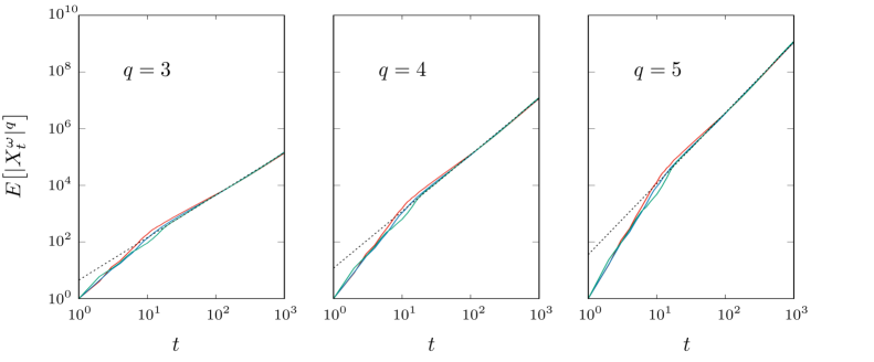
Figure 1: Quenched moments $E[|X_{t}^{\omega}|^{q}]$ versus time $t$ in log-log scale for $q=3$ (left), $q=4$ (center), and $q=5$ (right). For each $q$, three different samples $\omega$ corresponding to different colors are considered and the black dotted line is the moment $g_{q}t^{\frac{q}{2}}$ of the Brownian motion rescaled by $\mu$. Here the model is defined by the Pareto’s law $\mathbb{P}[\Delta_{1}>x]:=(x\vee 1)^{-\alpha}$ for $x>0$ with $\alpha=2$, which gives $\mu=2$, and the quenched moments are estimated by averaging over $10^{10}$ simulated particle trajectories.

In the light of our findings, asymptotic superdiffusion in individual samples, if any, necessarily requires that the interdistances between scattering points have infinite mean $\mu$. Whether or not the hypothesis $\mu=+\infty$ is sufficient to observe quenched superdiffusion is left as a completely open problem to be investigated in future research. We conjecture that the quenched $q$-order moments may exhibit a scaling law in time with a deterministic exponent as in Theorem 6 even in the case $\mu=+\infty$, similarly to what was previously found by the author [58] in the context of self-similar Lévy processes, but this time the coefficient $g_{q}$ may depend on the sample environment. Returning to the case $\mu<+\infty$, while identifying the nature of diffusion in different frameworks, this work raises a new question about how the transition from the quenched normal diffusion to the annealed superdiffusion occurs. The transition from the annealed to the quenched asymptotics has been addressed in other contexts, such as sums of random exponentials [8], random walks among random traps [10], and the parabolic Anderson model [32, 38]. In these cases, the approach used by the authors was to average the random field of interest over a box of increasing size with time, thus introducing a new parameter that rules the size growth and governs the quenched to annealed transition. As far as the Lévy-Lorentz gas is concerned, in order to study the quenched to annealed transition one may consider to average the process over an increasing pool of environment realizations. Work is in progress along this line. As a final curious remark, we point out that large differences between individual samples were observed in the experiments by Barthelemy, Bertolotti, and Wiersma [4] on the transmitted light in Lévy glasses, and for this reason they were prompted to average over a set of 900 disorder realizations. This probably means that their experimental results lie somewhere between the quenched and the annealed regime.

3 Preliminaries to the proofs of the main theorems

This section is devoted to some preparatory results for the proof of Theorems 3, 4, 5, and 6. For $r\in\mathbb{Z}$, let us say that the edge $r$ is between points $r-1$ and $r$ and, for $n\geq 1$, let us denote by $R_{n}$ the edge that the simple symmetric random walk covers in the $n$th jump:

$$R_{n}:=\frac{1+S_{n-1}+S_{n}}{2}.$$

For each $n\geq 1$ and $r\in\mathbb{Z}$, let us consider the local time $U_{n,r}$ on the edge $r$ given by

$$U_{n,r}:=\sum_{k=1}^{n}\mathds{1}_{\{R_{k}=r\}}~{}~{}~{}~{}~{}(U_{0,r}:=0).$$

The variables $R_{n}$ and $U_{n,r}$ are originally defined on the probability space $(\mathcal{S},\mathfrak{S},P)$ of velocities. We make use of them to recast the $n$th collision time as

$$T_{n}^{\omega}:=\sum_{k=1}^{n}|\omega_{S_{k}}-\omega_{S_{k-1}}|=\sum_{k=1}^{n}|\omega_{R_{k}}-\omega_{R_{k}-1}|=\sum_{k=1}^{n}\Delta^{\omega}_{R_{k}}=\sum_{r=-\infty}^{+\infty}\Delta_{r}^{\omega}U_{n,r}.$$

Our habit of denoting with same symbols both the variables defined on $(\mathcal{S},\mathfrak{S},P)$, or $(\Omega,\mathscr{F},\mathbb{P})$, and their natural extensions over the product probability space $(\Omega\times\mathcal{S},\mathscr{F}\times\mathfrak{S},\mathbb{P}\times P)$ allows us to write $T_{n}=\sum_{k=1}^{n}\Delta_{R_{k}}=\sum_{r=-\infty}^{+\infty}\Delta_{r}U_{n,r}$. Let us point out that this habit also justifies the writing of certain formulas involving probability measures and projections, such as $\mathbb{P}\times P[R_{n}>0]=P[R_{n}>0]$ or $\mathbb{E}\times E[\Delta_{r}]=\mathbb{E}[\Delta_{r}]$.

In Section 3.1 we propose some standard bounds for the variables $R_{n}$ and $U_{n,r}$, moving their proofs to sections of the appendix. These bounds are employed in Section 3.2 to achieve an annealed and a quenched large deviation estimate for collision times.

3.1 Jumps and local time on edges

Set $M_{n}^{+}:=\max\{R_{1},\ldots,R_{n}\}$ and $M_{n}^{-}:=\min\{R_{1},\ldots,R_{n}\}$ for each $n\geq 1$. The first result we list supplies the distribution of these random variables and is proved in Appendix B. Let us observe that $0\leq M_{n}^{+}\leq n$, as $R_{1}\geq 0$ and $R_{k}\leq k$ for all $k$, and that $-n<M_{n}^{-}\leq 1$, as $R_{1}\leq 1$ and $R_{k}\geq-k$ for all $k$. Hereafter we make the convention that the binomial coefficient ${n\choose k}$ is $0$ if $k>n$.

Proposition 1.

The following conclusions hold:

1. $\{M_{n}^{-}\}_{n\in\mathbb{Z}_{\geq 1}}$ and $\{1-M_{n}^{+}\}_{n\in\mathbb{Z}_{\geq 1}}$ share the same finite-dimensional distributions under the law $P$;

2. for every integers $n\geq 1$ and $m\geq 0$

   $$P\big{[}M_{n}^{+}=m\big{]}=\frac{1}{2^{n}}{n\choose\lfloor\frac{n+m+1}{2}\rfloor}.$$

The tail distribution of $M_{n}^{+}$ is described by the following lemma, whose proof is reported in Appendix C.

Lemma 3.

For every integer $n\geq 1$ and real number $L>0$

$$P\big{[}M_{n}^{+}>L\big{]}\leq 2e^{-\frac{L^{2}}{2n}}.$$

The next lemma provides an upper bound for the moments of $M_{n}^{+}$ and is demonstrated in Appendix D.

Lemma 4.

For every integer $n\geq 1$ and real number $q>0$

$$E\big{[}(M_{n}^{+})^{q}\big{]}\leq 2(qn)^{\frac{q}{2}}.$$

The local time $U_{n,r}$ on the edge $r$ is a random variable taking non-negative integer values. We point out that $U_{n,r}=0$ unless $-n<r\leq n$ and that $\sum_{r=-\infty}^{+\infty}U_{n,r}=n$. The following proposition provides the distribution of $U_{n,r}$. The proof is presented in Appendix E.

Proposition 2.

The following conclusions hold for every integer $n\geq 1$:

1. $\{U_{n,1-r}\}_{r\in\mathbb{Z}}$ and $\{U_{n,r}\}_{r\in\mathbb{Z}}$ share the same finite-dimensional distributions under the law $P$;

2. for all $r\geq 1$ and $u\geq 0$

   $$P\big{[}U_{n,r}=u\big{]}=\begin{cases}1-\frac{1}{2^{n}}\sum_{k=1}^{+\infty}{n\choose\lfloor\frac{n+r+k}{2}\rfloor}&\mbox{if }u=0,\\ \frac{1}{2^{n}}{n\choose\lfloor\frac{n+r+u}{2}\rfloor}&\mbox{if }u\geq 1.\end{cases}$$

Based on the exact results of Proposition 2, the next lemma provides an estimate of the probability that at least one among the $U_{n,r}$’s with different $r$ exceeds a given threshold. It is proved in Appendix F.

Lemma 5.

For every integer $n\geq 1$ and real number $L>0$

$$P\Big{[}\max_{r\in\mathbb{Z}}\{U_{n,r}\}>L\Big{]}\leq 4ne^{-\frac{L^{2}}{2n}}.$$

3.2 Collision times

The law of large numbers for collision times stated by Theorem 1 implies that $\mathbb{P}\times P[T_{n}\leq\gamma n]$ goes to zero as $n$ goes to infinity for each $\gamma<\mu$. We now use Lemma 5 to investigate how zero is approached when $\mu<+\infty$.

Lemma 6.

Assume that $\mu<+\infty$. For each $\gamma<\mu$ there exists $\kappa>0$ such that for all sufficiently large $n$

$$\mathbb{P}\times P\big{[}T_{n}\leq\gamma n\big{]}\leq e^{-\kappa n^{1/3}}.$$

Proof of Lemma 6.

Fix $n\geq 1$. Pick $\gamma<\mu$ and two real numbers $L>0$ and $\lambda>0$. By making use of the bound $\mathds{1}_{\{T_{n}\leq\gamma n\}}\leq e^{\lambda\gamma n-\lambda T_{n}}$ and Lemma 5 we find

$$\mathbb{P}\times P\big{[}T_{n}\leq\gamma n\big{]} \leq\mathbb{E}\times E\bigg{[}\mathds{1}_{\{T_{n}\leq\gamma n\}}\prod_{r\in\mathbb{Z}}\mathds{1}_{\{U_{n,r}\leq L\}}\bigg{]}+P\Big{[}\max_{r\in\mathbb{Z}}\{U_{n,r}>L\}\Big{]}$$

$$\leq e^{\lambda\gamma n}\,\mathbb{E}\times E\bigg{[}e^{-\lambda T_{n}}\prod_{r\in\mathbb{Z}}\mathds{1}_{\{U_{n,r}\leq L\}}\bigg{]}+4ne^{-\frac{L^{2}}{2n}}.$$

Then, the identity $T_{n}=\sum_{r=-\infty}^{+\infty}\Delta_{r}U_{n,r}$ and Fubini’s theorem yield

$$\mathbb{P}\times P\big{[}T_{n}\leq\gamma n\big{]} \leq e^{\lambda\gamma n}\,\mathbb{E}\times E\Bigg{[}\prod_{r=-\infty}^{+\infty}\sum_{u=0}^{\lfloor L\rfloor}e^{-\lambda\Delta_{r}u}\,\mathds{1}_{\{U_{n,r}=u\}}\Bigg{]}+4ne^{-\frac{L^{2}}{2n}}$$

$$=e^{\lambda\gamma n}E\Bigg{[}\prod_{r=-\infty}^{+\infty}\sum_{u=0}^{\lfloor L\rfloor}\mathbb{E}\big{[}e^{-\lambda\Delta_{1}u}\big{]}\mathds{1}_{\{U_{n,r}=u\}}\Bigg{]}+4ne^{-\frac{L^{2}}{2n}}.$$ (5)

The monotone convergence theorem tells us that $\lim_{\eta\uparrow+\infty}\mathbb{E}[\min\{\Delta_{1},\eta\}]=\mu$, so that there exists $\eta>0$ with the property that $\mathbb{E}[\min\{\Delta_{1},\eta\}]\geq(\mu+\gamma)/2$ as $\gamma<\mu$. Since $1-z\leq e^{-z}\leq 1-z+z^{2}/2$ for every $z\geq 0$, we have for each $u\geq 0$

$$\mathbb{E}\big{[}e^{-\lambda\Delta_{1}u}\big{]}\leq\mathbb{E}\big{[}e^{-\lambda\min\{\Delta_{1},\eta\}u}\big{]}\leq 1-\frac{\lambda(\mu+\gamma)}{2}u+\frac{\lambda^{2}\eta^{2}}{2}u^{2}\leq e^{-\lambda\frac{\mu+\gamma}{2}u+\frac{\lambda^{2}\eta^{2}}{2}u^{2}}.$$ (6)

By combining (5) with (6) and by recalling that $\sum_{r=-\infty}^{+\infty}U_{n,r}=n$ we get

$$\mathbb{P}\times P\big{[}T_{n}\leq\gamma n\big{]} \leq e^{\lambda\gamma n}\,E\Bigg{[}\prod_{r=-\infty}^{+\infty}\sum_{u=0}^{\lfloor L\rfloor}e^{-\frac{\lambda(\mu+\gamma)}{2}u+\frac{\lambda^{2}\eta^{2}L}{2}u}\,\mathds{1}_{\{U_{n,r}=u\}}\Bigg{]}+4ne^{-\frac{L^{2}}{2n}}$$

$$\leq e^{\lambda\gamma n}\,E\bigg{[}\prod_{r=-\infty}^{+\infty}e^{-\frac{\lambda(\mu+\gamma)}{2}U_{n,r}+\frac{\lambda^{2}\eta^{2}L}{2}U_{n,r}}\bigg{]}+4ne^{-\frac{L^{2}}{2n}}=e^{-\frac{\lambda(\mu-\gamma)}{2}n+\frac{\lambda^{2}\eta^{2}L}{2}n}+4ne^{-\frac{L^{2}}{2n}}.$$

At this point, by optimizing over $\lambda$, that is by taking $\lambda=(\mu-\gamma)/(2\eta^{2}L)$, we find

$$\mathbb{P}\times P\big{[}T_{n}\leq\gamma n\big{]}\leq e^{-\frac{(\mu-\gamma)^{2}}{8\eta^{2}L}n}+4ne^{-\frac{L^{2}}{2n}}.$$

The lemma is proved by choosing $L$ proportional to $n^{2/3}$. ∎

The same estimate of Lemma 6 applies to typical realizations of the environment, as stated by the following result.

Lemma 7.

Assume that $\mu<+\infty$. For each $\gamma<\mu$ there exists $\kappa>0$ such that the following property holds for $\mathbb{P}\mbox{-a.e.\ }\omega$: for all sufficiently large $n$

$$P\big{[}T_{n}^{\omega}\leq\gamma n\big{]}\leq e^{-\kappa n^{1/3}}.$$

Proof of Lemma 7.

Pick $\gamma<\mu$. Lemma 6 tells us that there exists a number $\kappa>0$ such that $\mathbb{P}\times P[T_{n}\leq\gamma n]\leq e^{-2\kappa n^{1/3}}$ for $n$ large enough. Let $\mathsf{Z}_{n}$ be the positive random variable on $(\Omega,\mathscr{F},\mathbb{P})$ that associates each $\omega$ with $e^{\kappa n^{1/3}}P[T_{n}^{\omega}\leq\gamma n]$. By invoking Fubini’s theorem, we find for all sufficiently large $n$

$$\mathbb{E}[\mathsf{Z}_{n}]=e^{\kappa n^{1/3}}\int_{\Omega}P\big{[}T_{n}^{\omega}\leq\gamma n\big{]}\,\mathbb{P}[d\omega]=e^{\kappa n^{1/3}}\,\mathbb{P}\times P\big{[}T_{n}\leq\gamma n\big{]}\leq e^{-\kappa n^{1/3}}.$$

This bound gives $\sum_{n=1}^{+\infty}\mathbb{P}[\mathsf{Z}_{n}>\epsilon]\leq(1/\epsilon)\sum_{n=1}^{+\infty}\mathbb{E}[\mathsf{Z}_{n}]<+\infty$ for every $\epsilon>0$ thanks to Markov’s inequality, which implies $\lim_{n\uparrow+\infty}\mathsf{Z}_{n}=0$ $\mathbb{P}$-a.s. by the Borel-Cantelli lemma. The fact that $\lim_{n\uparrow+\infty}e^{\kappa n^{1/3}}P[T_{n}^{\omega}\leq\gamma n]=0$ for $\mathbb{P}\mbox{-a.e.\ }\omega$ suffices to prove the lemma. ∎

4 Annealed fluctuations: proof of Theorem 3

The proof of Theorem 3 is driven by the idea that a large fluctuation of the particle displacement $X_{t}$ at a certain time $t$ is determined by a large fluctuation of the current edge along which the particle is traveling. The current edge and the current velocity are $R_{N_{t}}$ and $V_{N_{t}}$, respectively, where $N_{t}\geq 1$ is the label of the first collision after time $t$:

$$N_{t}:=\inf\big{\{}n\geq 1\,:\,T_{n}>t\big{\}}.$$

By definition, $N_{t}$ is the unique positive integer that satisfies $T_{N_{t}-1}\leq t<T_{N_{t}}$, and $N_{t}-1$ is the number of collisions up to time $t$. The edge corresponding to the current edge can be traveled back and forth several times before $t$, but ultimately its net contribution to the particle displacement $X_{t}$ is

$$\tau_{t}:=\begin{cases}\mathds{1}_{\{V_{N_{t}}=-1\}}(T_{N_{t}}-t)+\mathds{1}_{\{V_{N_{t}}=1\}}(t-T_{N_{t}-1})&\mbox{if }R_{N_{t}}\geq 1,\\ \mathds{1}_{\{V_{N_{t}}=-1\}}(t-T_{N_{t}-1})+\mathds{1}_{\{V_{N_{t}}=1\}}(T_{N_{t}}-t)&\mbox{if }R_{N_{t}}\leq 0.\end{cases}$$ (7)

The edges that the particle has completely covered by time $t$ and that together with $\tau_{t}$ determine the displacement $X_{t}$ are those from $1$ to $R_{N_{t}}-1$ if $R_{N_{t}}>1$ and those from $R_{N_{t}}+1$ to $0$ if $R_{N_{t}}<0$. Starting from (1), simple algebra actually allows one to verify that

$$X_{t}=\begin{cases}+\sum_{k=1}^{S_{N_{t}-1}}\Delta_{k}+V_{N_{t}}(t-T_{N_{t}-1})&\mbox{if }S_{N_{t}-1}\geq 1,\\ -\sum_{k=S_{N_{t}-1}+1}^{0}\Delta_{k}+V_{N_{t}}(t-T_{N_{t}-1})&\mbox{if }S_{N_{t}-1}\leq 0\end{cases}=\begin{cases}+\sum_{k=1}^{R_{N_{t}}-1}\Delta_{k}+\tau_{t}&\mbox{if }R_{N_{t}}\geq 1,\\ -\sum_{k=R_{N_{t}}+1}^{0}\Delta_{k}-\tau_{t}&\mbox{if }R_{N_{t}}\leq 0.\end{cases}$$ (8)

Hereafter we make the usual convention that an empty sum is 0 and an empty product is 1. We point out that the rigid constraint $T_{N_{t}-1}\leq t<T_{N_{t}}$ yields the bounds $0\leq\tau_{t}\leq T_{N_{t}}-T_{N_{t}-1}=\Delta_{R_{N_{t}}}$. It follows in particular from (8) that $0\leq X_{t}\leq\sum_{k=1}^{R_{N_{t}}}\Delta_{k}$ or $-\sum_{k=R_{N_{t}}}^{0}\Delta_{k}\leq X_{t}\leq 0$ depending on whether $R_{N_{t}}\geq 1$ or $R_{N_{t}}\leq 0$.

Now that the current edge has been characterized, let us outline our strategy to prove Theorem 3. Fix arbitrary real numbers $\delta\in(0,1]$ and $h\in(1/2,1)$. Pick $x\in[\delta,1]$ and observe that the condition $X_{t}>xt>0$ implies $R_{N_{t}}\geq 1$, since $X_{t}\leq 0$ when $R_{N_{t}}\leq 0$. Based on the bounds

$$\mathbb{P}\times P\big{[}\tau_{t}>xt,\,R_{N_{t}}\geq 1\big{]}\leq\mathbb{P}\times P\big{[}X_{t}>xt\big{]}\leq\mathbb{P}\times P\big{[}X_{t}>xt,\,\tau_{t}\leq hxt\big{]}+\mathbb{P}\times P\big{[}\tau_{t}>hxt,\,R_{N_{t}}\geq 1\big{]},$$ (9)

we shall show that a large fluctuation of $X_{t}$ is entirely determined by a large fluctuation of $\tau_{t}$. Specifically, we will verify by exact computation that the probability that $\tau_{t}$ takes a value of the order of magnitude of $t$ is of the order of magnitude of $\sqrt{t}\,\mathbb{P}[\Delta_{1}>t]$, whereas the probability $\mathbb{P}\times P[X_{t}>xt,\,\tau_{t}\leq hxt]$ of a large fluctuation of $X_{t}$ that cannot be ascribed to $\tau_{t}$ is negligible with respect to $\sqrt{t}\,\mathbb{P}[\Delta_{1}>t]$. Regarding the latter, we stress that the conditions $X_{t}>xt$ and $\tau_{t}\leq hxt$ entail $R_{N_{t}}\geq 2$, as $X_{t}=\tau_{t}$ when $R_{N_{t}}=1$ according to (8). They also imply $\sum_{k=1}^{R_{N_{t}}-1}\Delta_{k}=X_{t}-\tau_{t}>(1-h)xt\geq(1-h)\delta t$. Thus, setting $\eta:=(1-h)\delta>0$ for brevity, we have

$$\mathbb{P}\times P\big{[}X_{t}>xt,\,\tau_{t}\leq hxt\big{]} \leq\mathbb{P}\times P\Bigg{[}\sum_{k=1}^{R_{N_{t}}-1}\Delta_{k}>\eta t,\,R_{N_{t}}\geq 2\Bigg{]}$$

$$\leq\mathbb{P}\times P\Bigg{[}\sum_{k=1}^{R_{N_{t}}-1}\Delta_{k}>\eta t,\,\max\big{\{}\Delta_{1},\ldots,\Delta_{R_{N_{t}}-1}\big{\}}\leq\eta t/2,\,R_{N_{t}}\geq 2\Bigg{]}$$

$$+\mathbb{P}\times P\Big{[}\max\big{\{}\Delta_{1},\ldots,\Delta_{R_{N_{t}}-1}\big{\}}>\eta t/2,\,R_{N_{t}}\geq 2\Big{]}.$$ (10)

Inequality (10) constitutes our starting point to prove that the probability $\mathbb{P}\times P[X_{t}>xt,\,\tau_{t}\leq hxt]$ is negligible with respect to $\sqrt{t}\,\mathbb{P}[\Delta_{1}>t]$ by drawing attention to two distinct imperatives: there must be a long gap, which cannot be different from the current edge. In fact, the principle of a single big jump for i.i.d. heavy-tailed random variables suggests that a fluctuation of $\sum_{k=1}^{R_{N_{t}}-1}\Delta_{k}$ larger than $\eta t$ requires a comparable fluctuation of one of the summands. We will verify this fact by showing that the first term of the r.h.s. of (10) is suppressed by the constraint $\max\{\Delta_{1},\ldots,\Delta_{R_{N_{t}}-1}\}\leq\eta t/2$. On the other hand, as the summands are the lengths of the edges that the particle has traveled in the past, when one of them is allowed for a large fluctuation, i.e. when $\max\{\Delta_{1},\ldots,\Delta_{R_{N_{t}}-1}\}>\eta t/2$, the particle experiences the circumstance of not currently being on the edge with the largest length. This circumstance turns out to be very unlikely, meaning that the particle spends most of the time on the current edge after reaching it for the first time. We shall demonstrate this fact by proving that also the second term of the r.h.s. of (10) is negligible. The mechanism by which the particle remains confined to the current edge, traveling back and forth on it, is that the many close collisions involving the particle as it leaves the longest edge send it back very quickly.

When evaluating all terms in (9) and (10) we can restrict to events for which the number of collisions by time $t$ has at most order of magnitude of $t/\mu$, as it is very unlikely that $N_{t}$ takes larger values. In fact, we can cut off $N_{t}$ at $b_{t}:=\lfloor 2t/\mu\rfloor+1$ since Lemma 6 tells us that there exists a real number $\kappa>0$ such that for all sufficiently large $t$

$$\mathbb{P}\times P\big{[}N_{t}>b_{t}\big{]}=\mathbb{P}\times P\big{[}T_{b_{t}}\leq t\big{]}\leq\mathbb{P}\times P\big{[}T_{b_{t}}\leq\mu b_{t}/2\big{]}\leq e^{-\kappa b_{t}^{1/3}}.$$ (11)

By combining (9) and (10) we get for any $x\in[\delta,1]$

$$\Psi_{t}(x)\leq\mathbb{P}\times P\big{[}X_{t}>xt\big{]}\leq\Theta_{t}+\Phi_{t}+\Psi_{t}(hx)+3\,\mathbb{P}\times P\big{[}N_{t}>b_{t}\big{]}$$ (12)

with

$$\Theta_{t}:=\mathbb{P}\times P\Bigg{[}\sum_{k=1}^{R_{N_{t}}-1}\Delta_{k}>\eta t,\,\max\big{\{}\Delta_{1},\ldots,\Delta_{R_{N_{t}}-1}\big{\}}\leq\eta t/2,\,R_{N_{t}}\geq 2,\,N_{t}\leq b_{t}\Bigg{]},$$

$$\Phi_{t}:=\mathbb{P}\times P\Big{[}\max\big{\{}\Delta_{1},\ldots,\Delta_{R_{N_{t}}-1}\big{\}}>\eta t/2,\,R_{N_{t}}\geq 2,\,N_{t}\leq b_{t}\Big{]},$$

and

$$\Psi_{t}(y):=\mathbb{P}\times P\Big{[}\tau_{t}>yt,\,R_{N_{t}}\geq 1,\,N_{t}\leq b_{t}\Big{]}.$$

In Section 4.1 we shall make use of the precise large deviation principle (4) to show that

$$\lim_{t\uparrow+\infty}\frac{\Theta_{t}}{\sqrt{t}\,\mathbb{P}[\Delta_{1}>t]}=0.$$ (13)

In Section 4.2 we will prove that

$$\lim_{t\uparrow+\infty}\frac{\Phi_{t}}{\sqrt{t}\,\mathbb{P}[\Delta_{1}>t]}=0.$$ (14)

Finally, in Section 4.3 we shall demonstrate that

$$\adjustlimits{\lim}_{t\uparrow+\infty}{\sup}_{~{}y\in[\delta/2,1]~{}}\!\Bigg{\{}\bigg{|}\frac{\Psi_{t}(y)}{\sqrt{t}\,\mathbb{P}[\Delta_{1}>t]}-F(y)\bigg{|}\Bigg{\}}=0,$$ (15)

where for each $y\in(0,1]$

$$F(y):=\frac{1}{\sqrt{2\pi\mu}}\int_{y}^{1}f_{\alpha}\bigg{(}\frac{y}{\xi}\bigg{)}\frac{d\xi}{\xi^{\alpha}\sqrt{1-\xi}},$$ (16)

$f_{\alpha}$ being the function defined by (3). In Section 4.4 we shall verify that

$$\sup_{x\in[\delta,1]}\Big{\{}F(hx)-F(x)\Big{\}}\leq\frac{\sqrt{1-h}+h^{1-\alpha}-1}{\sqrt{\mu}\,(\delta/2)^{\alpha}}.$$ (17)

Since the tail probability of $\Delta_{1}$ is dominated from below by polynomials due to regular variation (see [15], Proposition 1.3.6), bound (11) gives

$$\lim_{t\uparrow+\infty}\frac{\mathbb{P}\times P[N_{t}>b_{t}]}{\sqrt{t}\,\mathbb{P}[\Delta_{1}>t]}=0.$$ (18)

In conclusion, (12) in combination with the limits (13), (14), (15), and (18) and the estimate (17) shows that

$$\adjustlimits{\limsup}_{t\uparrow+\infty}{\sup}_{x\in[\delta,1]}\Bigg{\{}\bigg{|}\frac{\mathbb{P}\times P[X_{t}>xt]}{\sqrt{t}\,\mathbb{P}[\Delta_{1}>t]}-F(x)\bigg{|}\Bigg{\}}\leq\frac{\sqrt{1-h}+h^{1-\alpha}-1}{\sqrt{\mu}\,(\delta/2)^{\alpha}}.$$

Theorem 3 follows from here by sending $h$ to 1. Limit (13) provides a rigorous interpretation of the principle of a single big jump in the context of the Lévy-Lorentz gas by demonstrating that large fluctuations of the particle displacement cannot be observed in the absence of large fluctuations of a single edge. Limit (14) confirms that it is very unlikely that there is an edge that exhibits a large fluctuation, but that this is not the current edge.

4.1 The limit (13) for $\Theta_{t}$

The first step to prove the limit (13) is to eliminate the random variable $N_{t}$ from $\Theta_{t}$. Bearing in mind that $\max\{R_{1},\ldots,R_{b_{t}}\}=M_{b_{t}}^{+}$, for each $t>0$ we have

$$\Theta_{t} :=\mathbb{P}\times P\Bigg{[}\sum_{k=1}^{R_{N_{t}}-1}\Delta_{k}>\eta t,\,\max\big{\{}\Delta_{1},\ldots,\Delta_{R_{N_{t}}-1}\big{\}}\leq\eta t/2,\,R_{N_{t}}\geq 2,\,N_{t}\leq b_{t}\Bigg{]}$$

$$\leq\mathbb{P}\times P\Bigg{[}\sum_{k=1}^{R_{N_{t}}-1}\min\big{\{}\Delta_{k},\eta t/2\big{\}}>\eta t,\,R_{N_{t}}\geq 2,\,N_{t}\leq b_{t}\Bigg{]}$$

$$\leq\mathbb{P}\times P\Bigg{[}\sum_{k=1}^{M_{b_{t}}^{+}}\min\big{\{}\Delta_{k},\eta t/2\big{\}}>\eta t,\,M_{b_{t}}^{+}\geq 2\Bigg{]}\leq\Theta_{t}^{\prime}+\Theta_{t}^{\prime\prime}$$ (19)

with

$$\Theta_{t}^{\prime}:=\mathbb{P}\times P\Bigg{[}\sum_{k=1}^{M_{b_{t}}^{+}}\min\big{\{}\Delta_{k},\eta t/2\big{\}}>\eta t,\,\max\big{\{}\Delta_{1},\ldots,\Delta_{M_{b_{t}}^{+}}\big{\}}>\eta t,\,M_{b_{t}}^{+}\geq 2\Bigg{]}$$

and

$$\Theta_{t}^{\prime\prime}:=\mathbb{P}\times P\Bigg{[}\sum_{k=1}^{M_{b_{t}}^{+}}\Delta_{k}>\eta t,\,\max\big{\{}\Delta_{1},\ldots,\Delta_{M_{b_{t}}^{+}}\big{\}}\leq\eta t,\,M_{b_{t}}^{+}\geq 1\Bigg{]}.$$

The bound (19) shows that (13) follows if we demonstrate that

$$\lim_{t\uparrow+\infty}\frac{\Theta_{t}^{\prime}}{\sqrt{t}\,\mathbb{P}[\Delta_{1}>t]}=\lim_{t\uparrow+\infty}\frac{\Theta_{t}^{\prime\prime}}{\sqrt{t}\,\mathbb{P}[\Delta_{1}>t]}=0.$$ (20)

The first limit of (20) is immediate. Since the condition $\max\{\Delta_{1},\ldots,\Delta_{m}\}>\eta t$ with $m\geq 2$ entails that at least one variable among the i.i.d. random variables $\Delta_{1},\ldots,\Delta_{m}$ is larger that $\eta t$, we can write

$$\Theta_{t}^{\prime} \leq\sum_{m=2}^{+\infty}\sum_{l=1}^{m}\mathbb{P}\times P\Bigg{[}\sum_{k=1}^{m}\min\big{\{}\Delta_{k},\eta t/2\big{\}}>\eta t,\,\Delta_{l}>\eta t,\,M_{b_{t}}^{+}=m\Bigg{]}$$

$$\leq\sum_{m=2}^{+\infty}m\,\mathbb{P}\times P\Bigg{[}\sum_{k=1}^{m-1}\Delta_{k}>\eta t/2,\,\Delta_{m}>\eta t,\,M_{b_{t}}^{+}=m\Bigg{]}$$

$$=\mathbb{P}\big{[}\Delta_{1}>\eta t\big{]}\sum_{m=2}^{+\infty}m\,\mathbb{P}\Bigg{[}\sum_{k=1}^{m-1}\Delta_{k}>\eta t/2\Bigg{]}P\big{[}M_{b_{t}}^{+}=m\big{]}.$$

At this point, an application of Markov’s inequality and Lemma 4 give for all $t$

$$\Theta_{t}^{\prime}\leq\mathbb{P}\big{[}\Delta_{1}>\eta t\big{]}\sum_{m=2}^{+\infty}\frac{2\mu m(m-1)}{\eta t}P\big{[}M_{b_{t}}^{+}=m\big{]}\leq\frac{2\mu E[(M_{b_{t}}^{+})^{2}]}{\eta t}\,\mathbb{P}\big{[}\Delta_{1}>\eta t\big{]}\leq\frac{8\mu b_{t}}{\eta t}\,\mathbb{P}\big{[}\Delta_{1}>\eta t\big{]}.$$

The limit (20) for $\Theta_{t}^{\prime}$ follows from here since $b_{t}$ is of the order of magnitude of $t$ and $\lim_{t\uparrow+\infty}\mathbb{P}[\Delta_{1}>\eta t]/\mathbb{P}[\Delta_{1}>t]=\eta^{-\alpha}<+\infty$ by regular variation.

The second limit of (20) involves the precise large deviation principle (4) for the interdistances between scatterers. In a nutshell, $\Theta_{t}^{\prime\prime}$ is negligible with respect to $\sqrt{t}\,\mathbb{P}[\Delta_{1}>t]$ because a fluctuation of $\sum_{k=1}^{M_{b_{t}}^{+}}\Delta_{k}$ lager than $\eta t$ is realized by a comparable fluctuation of one of the summands, but this is impossible under the constraint $\max\{\Delta_{1},\ldots,\Delta_{M_{b_{t}}^{+}}\}\leq\eta t$. In order to get at a rigorous proof, let us notice at first that the condition $\max\{\Delta_{1},\ldots,\Delta_{M_{b_{t}}^{+}}\}>\eta t$ entails $\sum_{k=1}^{M_{b_{t}}^{+}}\Delta_{k}>\eta t$, so that

$$\Theta_{t}^{\prime\prime}=\mathbb{P}\times P\Bigg{[}\sum_{k=1}^{M_{b_{t}}^{+}}\Delta_{k}>\eta t,\,M_{b_{t}}^{+}\geq 1\Bigg{]}-\mathbb{P}\times P\Bigg{[}\max\big{\{}\Delta_{1},\ldots,\Delta_{M_{b_{t}}^{+}}\big{\}}>\eta t,\,M_{b_{t}}^{+}\geq 1\Bigg{]}.$$ (21)

To address the first term of the r.h.s. of (21), pick an arbitrary real number $\epsilon\in(0,1/2)$. In the light of (4) with $\gamma=\mu$ there exists an integer $m_{o}\geq 1$ such that for all $m\geq m_{o}$ and $z\geq\mu m$

$$\mathbb{P}\Bigg{[}\sum_{k=1}^{m}\Delta_{k}>\mu m+z\Bigg{]}\leq m(1+\epsilon)\,\mathbb{P}\big{[}\Delta_{1}>z\big{]}.$$ (22)

Set $t_{o}:=\mu m_{o}/(\epsilon\eta)$. If $t>t_{o}$, then $\epsilon\eta t-\mu m_{o}>0$ and Lemma 3 shows that

$$P\big{[}\mu(M_{b_{t}}^{+}\vee m_{o})>\epsilon\eta t\big{]}\leq P\big{[}\mu M_{b_{t}}^{+}>\epsilon\eta t-\mu m_{o}\big{]}\leq 2e^{-\frac{(\epsilon\eta t-\mu m_{o})^{2}}{2\mu^{2}b_{t}}}.$$

Thus, if $m\geq 1$ satisfies $\mu(m\vee m_{o})\leq\epsilon\eta t$, then $\eta t-\mu(m\vee m_{o})\geq(1-\epsilon)\eta t>\epsilon\eta t\geq\mu(m\vee m_{o})$ as $\epsilon<1/2$ and (22) yields

$$\mathbb{P}\Bigg{[}\sum_{k=1}^{m}\Delta_{k}>\eta t\Bigg{]} \leq\mathbb{P}\Bigg{[}\sum_{k=1}^{m\vee m_{o}}\Delta_{k}>\eta t\Bigg{]}\leq\mathbb{P}\Bigg{[}\sum_{k=1}^{m\vee m_{o}}\Delta_{k}>\mu(m\vee m_{o})+(1-\epsilon)\eta t\Bigg{]}$$

$$\leq(m\vee m_{o})(1+\epsilon)\,\mathbb{P}\big{[}\Delta_{1}>(1-\epsilon)\eta t\big{]}\leq(m_{o}+m)(1+\epsilon)\,\mathbb{P}\big{[}\Delta_{1}>(1-\epsilon)\eta t\big{]}.$$

It follows that for every $t>t_{o}$

$$\mathbb{P}\times P\Bigg{[}\sum_{k=1}^{M_{b_{t}}^{+}}\Delta_{k}>\eta t,\,M_{b_{t}}^{+}\geq 1\Bigg{]} \leq\sum_{m=1}^{+\infty}\mathds{1}_{\big{\{}\mu(m\vee m_{o})\leq\epsilon\eta t\big{\}}}\,\mathbb{P}\Bigg{[}\sum_{k=1}^{m}\Delta_{k}>\eta t\Bigg{]}P\big{[}M_{b_{t}}^{+}=m\big{]}+P\big{[}\mu(M_{b_{t}}^{+}\vee m_{o})>\epsilon\eta t\big{]}$$

$$\leq(1+\epsilon)\,\mathbb{P}\big{[}\Delta_{1}>(1-\epsilon)\eta t\big{]}\Big{(}m_{o}+E\big{[}M_{b_{t}}^{+}\big{]}\Big{)}+2e^{-\frac{(\epsilon\eta t-\mu m_{o})^{2}}{2\mu^{2}b_{t}}}.$$ (23)

Furthermore, the independence of the interdistances and the inequality $1-(1-z)^{m}\geq mz-m^{2}z^{2}$ valid for every $m\geq 1$ and $z\in[0,1]$ give for all $t>0$

$$\mathbb{P}\times P\bigg{[}\max\big{\{}\Delta_{1},\ldots,\Delta_{M_{b_{t}}^{+}}\big{\}}>\eta t,\,M_{b_{t}}^{+}\geq 1\bigg{]} =\sum_{m=1}^{+\infty}\bigg{\{}1-\Big{(}1-\mathbb{P}\big{[}\Delta_{1}>\eta t\big{]}\Big{)}^{m}\bigg{\}}P\big{[}M_{b_{t}}^{+}=m\big{]}$$

$$\geq E\big{[}M_{b_{t}}^{+}\big{]}\mathbb{P}\big{[}\Delta_{1}>\eta t\big{]}-E\big{[}(M_{b_{t}}^{+})^{2}\big{]}\mathbb{P}\big{[}\Delta_{1}>\eta t\big{]}^{2}.$$ (24)

In conclusion, by combining (21) with (23) and (24) we realize that for all $t>t_{o}$

$$\Theta_{t}^{\prime\prime} \leq(1+\epsilon)\,\mathbb{P}\big{[}\Delta_{1}>(1-\epsilon)\eta t\big{]}\Big{(}m_{o}+E\big{[}M_{b_{t}}^{+}\big{]}\Big{)}-E\big{[}M_{b_{t}}^{+}\big{]}\mathbb{P}\big{[}\Delta_{1}>\eta t\big{]}$$

$$+E\big{[}(M_{b_{t}}^{+})^{2}\big{]}\mathbb{P}\big{[}\Delta_{1}>\eta t\big{]}^{2}+2e^{-\frac{(\epsilon\eta t-\mu m_{o})^{2}}{2\mu^{2}b_{t}}}$$

$$=m_{0}(1+\epsilon)\,\mathbb{P}\big{[}\Delta_{1}>(1-\epsilon)\eta t\big{]}+\epsilon E\big{[}M_{b_{t}}^{+}\big{]}\mathbb{P}\big{[}\Delta_{1}>(1-\epsilon)\eta t\big{]}+E\big{[}M_{b_{t}}^{+}\big{]}\mathbb{P}\big{[}(1-\epsilon)\eta t<\Delta_{1}\leq\eta t\big{]}$$

$$+E\big{[}(M_{b_{t}}^{+})^{2}\big{]}\mathbb{P}\big{[}\Delta_{1}>\eta t\big{]}^{2}+2e^{-\frac{(\epsilon\eta t-\mu m_{o})^{2}}{2\mu^{2}b_{t}}}$$

$$\leq m_{0}(1+\epsilon)\,\mathbb{P}\big{[}\Delta_{1}>(1-\epsilon)\eta t\big{]}+2\epsilon\sqrt{b_{t}}\,\mathbb{P}\big{[}\Delta_{1}>(1-\epsilon)\eta t\big{]}+2\sqrt{b_{t}}\,\mathbb{P}\big{[}(1-\epsilon)\eta t<\Delta_{1}\leq\eta t\big{]}$$

$$+\frac{4\mu b_{t}}{\eta t}\,\mathbb{P}\big{[}\Delta_{1}>\eta t\big{]}+2e^{-\frac{(\epsilon\eta t-\mu m_{o})^{2}}{2\mu^{2}b_{t}}},$$

where we have used Lemma 4 to bound the moments of $M_{b_{t}}^{+}$ and the Markov’s inequality to deduce $\mathbb{P}[\Delta_{1}>\eta t]\leq\mu/(\eta t)$. Regular variation implies $\lim_{t\uparrow+\infty}\mathbb{P}[\Delta_{1}>\beta t]/\mathbb{P}[\Delta_{1}>t]=\beta^{-\alpha}$ for any $\beta>0$, as well as the fact that $\mathbb{P}[\Delta_{1}>\cdot\,]$ is dominated from below by polynomials (see [15], Proposition 1.3.6). Then, recalling that $b_{t}:=\lfloor 2t/\mu\rfloor+1$, we find

$$\limsup_{t\uparrow+\infty}\frac{\Theta_{t}^{\prime\prime}}{\sqrt{t}\,\mathbb{P}[\Delta_{1}>t]}\leq\eta^{-\alpha}\sqrt{\frac{8}{\mu}}\bigg{[}\frac{1+\epsilon}{(1-\epsilon)^{\alpha}}-1\bigg{]}.$$

The arbitrariness of $\epsilon\in(0,1/2)$ proves the limit (20) for $\Theta_{t}^{\prime\prime}$.

4.2 The limit (14) for $\Phi_{t}$

Let us prove the limit (14) for $\Phi_{t}$. Since the condition $\max\{\Delta_{1},\ldots,\Delta_{r}\}>\eta t/2$ implies that at least one variable among $\Delta_{1},\ldots,\Delta_{r}$ exceeds $\eta t/2$, we can write down the bound

$$\Phi_{t} :=\mathbb{P}\times P\Big{[}\max\big{\{}\Delta_{1},\ldots,\Delta_{R_{N_{t}}-1}\big{\}}>\eta t/2,\,R_{N_{t}}\geq 2,\,N_{t}\leq b_{t}\Big{]}$$

$$=\sum_{r=1}^{+\infty}\,\mathbb{P}\times P\Big{[}\max\big{\{}\Delta_{1},\ldots,\Delta_{r}\big{\}}>\eta t/2,\,R_{N_{t}}=r+1,\,N_{t}\leq b_{t}\Big{]}$$

$$\leq\sum_{r=1}^{+\infty}\sum_{k=1}^{r}\,\mathbb{P}\times P\Big{[}\Delta_{k}>\eta t/2,\,R_{N_{t}}=r+1,\,N_{t}\leq b_{t}\Big{]}=\sum_{k=1}^{+\infty}\,\mathbb{P}\times P\Big{[}\Delta_{k}>\eta t/2,\,R_{N_{t}}>k,\,N_{t}\leq b_{t}\Big{]}.$$ (25)

Because of the constraint $1\leq k<R_{N_{t}}$, the last expression clearly states that an edge $k$ that determines the displacement of the particle at time $t$ contributes with a large fluctuation above $\eta t/2$, but this edge is not the current edge $R_{N_{t}}$. A second large fluctuation involving another edge is very unlikely, so that the particle undergoes many close collisions when it leaves the edge $k$. Actually, since the sequence $\{R_{n}\}_{n\in\mathbb{Z}_{>0}}$ with increments $-1$, $0$, or $1$ cannot reach a point larger than $k\geq 1$ without going through $k$ first, the condition $1\leq k<R_{N_{t}}$ implies that there exists a positive integer $n<N_{t}$ such that $R_{n}=k$ and $\min\{R_{n+1},\ldots,R_{N_{t}}\}>k$. This means that the particle passed on the longest edge $k$ one last time at the $n$th jump and then has no longer passed over this edge. Then, the reason why $\Phi_{t}$ is negligible with respect to $\sqrt{t}\,\mathbb{P}[\Delta_{1}>t]$ is that it is very improbable that the particle no longer comes back to the edge $k$ as a result of the many collisions between times $T_{n}$ and $T_{N_{t}-1}$.

Starting from (25), the naive implementation of these arguments leads us to the bound

$$\Phi_{t}\leq\sum_{k=1}^{+\infty}\sum_{n=1}^{b_{t}-1}\,\mathbb{P}\times P\bigg{[}\Delta_{k}>\eta t/2,\,R_{n}=k,\,\min\big{\{}R_{n+1},\ldots,R_{N_{t}}\big{\}}>k,\,n<N_{t}\leq b_{t}\bigg{]}.$$ (26)

The number $N_{t}$ is the complex mathematical object of (26) because of its dependence on the other random elements. With the purpose of resolving such dependence and eliminate $N_{t}$, we come back to (25) and do some preliminary manipulations to (26). As $N_{t}$ is the unique positive integer that satisfies $T_{N_{t}-1}\leq t<T_{N_{t}}$, the idea is to invert this relation in order to predict $N_{t}$. To do this, let us consider for each $n\geq 0$ a collision time $\mathsf{T}_{n,k}$ deprived of the time that the particle spends on a given edge $k\in\mathbb{Z}$:

$$\mathsf{T}_{n,k}:=T_{n}-\Delta_{k}U_{n,k}=\sum_{\begin{subarray}{c}r=-\infty\\ r\neq k\end{subarray}}^{+\infty}\Delta_{r}U_{n,r}.$$ (27)

The sequence $\{\mathsf{T}_{n,k}\}_{n\in\mathbb{Z}_{\geq 0}}$ is independent of $\Delta_{k}$ and non-decreasing, the latter being a property of local times on edges. The law of large numbers for collision times stated by Theorem 1 suggests that $\mathsf{T}_{n,k}/n$ may converge in probability to $\mu$ when $n$ is sent to infinity, even if the edge $k$ is affected by a large fluctuation. We have $T_{N_{t}-1}=\mathsf{T}_{N_{t}-1,k}+\Delta_{k}U_{N_{t}-1,k}$, with $U_{N_{t}-1,k}=U_{N_{t},k}-\mathds{1}_{\{R_{N_{t}}=k\}}=U_{N_{t},k}$ by definition if $k\neq R_{N_{t}}$, and $T_{N_{t}}=\mathsf{T}_{N_{t},k}+\Delta_{k}U_{N_{t},k}$, so that the constraint $T_{N_{t}-1}\leq t<T_{N_{t}}$ reads $\mathsf{T}_{N_{t}-1,k}\leq t-\Delta_{k}U_{N_{t},k}<\mathsf{T}_{N_{t},k}$ if $k\neq R_{N_{t}}$. The trick to invert this relation is to replace $\mathsf{T}_{N_{t}-1,k}/(N_{t}-1)$ and $\mathsf{T}_{N_{t},k}/N_{t}$ with $\mu$, and to show that such a replacement is justified. So, we pick a real number $\epsilon\in(0,1)$ and recast (25) as

$$\Phi_{t}\leq\Phi_{t}^{\prime}+\Phi_{t}^{\prime\prime}$$ (28)

with

$$\Phi_{t}^{\prime}:=\sum_{k=1}^{+\infty}\,\mathbb{P}\times P\Bigg{[}\Delta_{k}>\eta t/2,\,\bigg{|}\frac{\mathsf{T}_{N_{t}-1,k}}{N_{t}-1}-\mu\bigg{|}\vee\bigg{|}\frac{\mathsf{T}_{N_{t},k}}{N_{t}}-\mu\bigg{|}\leq\epsilon\mu,\,R_{N_{t}}>k\Bigg{]}$$ (29)

and

$$\Phi_{t}^{\prime\prime}:=\sum_{k=1}^{+\infty}\,\mathbb{P}\times P\Bigg{[}\Delta_{k}>\eta t/2,\,\bigg{|}\frac{\mathsf{T}_{N_{t}-1,k}}{N_{t}-1}-\mu\bigg{|}\vee\bigg{|}\frac{\mathsf{T}_{N_{t},k}}{N_{t}}-\mu\bigg{|}>\epsilon\mu,\,R_{N_{t}}>k,\,N_{t}\leq b_{t}\Bigg{]}.$$ (30)

Notice that we have dropped the condition $N_{t}\leq b_{t}$ when defining $\Phi_{t}^{\prime}$ because irrelevant.

The term $\Phi_{t}^{\prime}$ accounts for events where $|\mathsf{T}_{N_{t}-1,k}/(N_{t}-1)-\mu|\leq\epsilon\mu$ and $|\mathsf{T}_{N_{t},k}/N_{t}-\mu|\leq\epsilon\mu$. For these events the constraint $\mathsf{T}_{N_{t}-1,k}\leq t-\Delta_{k}U_{N_{t},k}<\mathsf{T}_{N_{t},k}$ implies $\Delta_{k}U_{N_{t},k}\leq t$ and $(1-\epsilon)\mu(N_{t}-1)\leq t-\Delta_{k}U_{N_{t},k}<(1+\epsilon)\mu N_{t}$. The latter is tantamount to $N_{t}\in(p_{t-\Delta_{k}U_{N_{t},k}},q_{t-\Delta_{k}U_{N_{t},k}}+1]$ with integers $p_{z}$ and $q_{z}$ defined for every $z\in\mathbb{R}$ by

$$p_{z}:=\bigg{\lfloor}\frac{z\vee 0}{(1+\epsilon)\mu}\bigg{\rfloor}\geq 0$$ (31)

and

$$q_{z}:=\bigg{\lfloor}\frac{z\vee 0}{(1-\epsilon)\mu}\bigg{\rfloor}\geq p_{z}.$$ (32)

We have thus conveniently inverted the relation $T_{N_{t}-1}\leq t<T_{N_{t}}$ and found a narrow interval that encloses $N_{t}$. These reasonings allow us to deduce from (29) that for every $t>0$

$$\Phi_{t}^{\prime} \leq\sum_{k=1}^{+\infty}\,\mathbb{P}\times P\bigg{[}\Delta_{k}>\eta t/2,\,N_{t}\in\big{(}p_{t-\Delta_{k}U_{N_{t},k}},q_{t-\Delta_{k}U_{N_{t},k}}+1\big{]},\,\Delta_{k}U_{N_{t},k}\leq t,\,R_{N_{t}}>k\bigg{]}$$

$$\leq\sum_{u=0}^{\lfloor 2/\eta\rfloor}\sum_{k=1}^{+\infty}\,\mathbb{P}\times P\bigg{[}\Delta_{k}>\eta t/2,\,N_{t}\in\big{(}p_{t-\Delta_{k}u},q_{t-\Delta_{k}u}+1\big{]},\,U_{N_{t},k}=u,\,R_{N_{t}}>k\bigg{]}.$$ (33)

At this point, we can recover the arguments that led to (26), namely that the condition $1\leq k<R_{N_{t}}$ entails that there exists a positive integer $n<N_{t}$ such that $R_{n}=k$ and $\min\{R_{n+1},\ldots,R_{N_{t}}\}>k$. This gives in particular $U_{N_{t},k}=U_{n,k}\geq 1$. The novelty is that we can now use that constraint $N_{t}\in(p_{t-\Delta_{k}u},q_{t-\Delta_{k}u}+1]$ to predict $N_{t}$ and to conclude that $n$ satisfies $n\leq q_{t-\Delta_{k}u}$, $R_{n}=k$, and $\min\{R_{n+1},\ldots,R_{n\vee p_{t-\Delta_{k}u}+1}\}>k$. Thus, we can replace (33) with

$$\Phi_{t}^{\prime} \leq\sum_{u=1}^{\lfloor 2/\eta\rfloor}\sum_{k=1}^{+\infty}\sum_{n=1}^{+\infty}\,\mathbb{P}\times P\bigg{[}\Delta_{k}>\eta t/2,\,n\leq q_{t-\Delta_{k}u},\,U_{n,k}=u,\,R_{n}=k,\,\min\big{\{}R_{n+1},\ldots,R_{n\vee p_{t-\Delta_{k}u}+1}\big{\}}>k\bigg{]}.$$

This bound is a version of (26) where $N_{t}$ has been resolved. Bearing in mind that $\Delta_{k}$ is distributed as $\Delta_{1}$, an application of Fubini’s theorem finally yields for any $t>0$

$$\Phi_{t}^{\prime} \leq\sum_{u=1}^{\lfloor 2/\eta\rfloor}\mathbb{E}\Bigg{[}\mathds{1}_{\{\Delta_{1}>\eta t/2\}}\sum_{n=1}^{q_{t-\Delta_{1}u}}\sum_{k=1}^{+\infty}\,P\Big{[}U_{n,k}=u,\,R_{n}=k,\,\min\big{\{}R_{n+1},\ldots,R_{n\vee p_{t-\Delta_{1}u}+1}\big{\}}>k\Big{]}\Bigg{]}$$

$$\leq\sum_{u=1}^{\lfloor 2/\eta\rfloor}\mathbb{E}\Big{[}\mathds{1}_{\{\Delta_{1}>\eta t/2\}}\,\mathcal{E}_{u}\big{\{}p_{t-\Delta_{1}u},q_{t-\Delta_{1}u}\big{\}}\Big{]},$$ (34)

where we have set

$$\mathcal{E}_{u}\{p,q\}:=\sum_{n=1}^{q}\,P\Big{[}U_{n,R_{n}}=u,\,\min\big{\{}R_{n+1},\ldots,R_{n\vee p+1}\big{\}}>R_{n}\Big{]}$$ (35)

for all integers $0\leq p\leq q$ and $u>0$. Through (34), we have reduced the problem to an estimate of $\mathcal{E}_{u}\{p,q\}$, which only involves the properties of the simple symmetric random walk. We let the following lemma, whose proof is provided in Appendix G, to tackle $\mathcal{E}_{u}\{p,q\}$. Basically, $\mathcal{E}_{u}\{p,q\}$ measures how likely it is that, at a given time, the particle is not on an edge it has visited a few times in the past.

Lemma 8.

Let $\mathcal{E}_{u}\{p,q\}$ by defined by (35) for every integers $0\leq p\leq q$ and $u>0$. Then

$$\mathcal{E}_{u}\{p,q\}\leq 5+\sqrt{q}-\sqrt{p+1}.$$

Lemma 8 and definitions (31) and (32) give for every positive $u$ and $t$

$$\mathcal{E}_{u}\big{\{}p_{t-\Delta_{1}u},q_{t-\Delta_{1}u}\big{\}}\leq 5+\sqrt{\frac{(t-\Delta_{1}u)\vee 0}{(1-\epsilon)\mu}}-\sqrt{\frac{(t-\Delta_{1}u)\vee 0}{(1+\epsilon)\mu}}\leq 5+\bigg{(}\frac{1}{\sqrt{1-\epsilon}}-\frac{1}{\sqrt{1+\epsilon}}\bigg{)}\sqrt{\frac{t}{\mu}}.$$

It follows from (34) that for all $t>0$

$$\Phi_{t}^{\prime}\leq\frac{10}{\eta}\,\mathbb{P}\big{[}\Delta_{1}>\eta t/2\big{]}+\frac{2}{\eta}\bigg{(}\frac{1}{\sqrt{1-\epsilon}}-\frac{1}{\sqrt{1+\epsilon}}\bigg{)}\sqrt{\frac{t}{\mu}}\,\mathbb{P}\big{[}\Delta_{1}>\eta t/2\big{]}.$$ (36)

Let us move to $\Phi_{t}^{\prime\prime}$. This term involves the deviations of the random variables $\mathsf{T}_{n,k}/n$ from $\mu$, which are not significant as we now show. To deal with $\Phi_{t}^{\prime\prime}$ it is convenient to distinguish events that account for few collisions from the others. Set $a_{t}:=\lfloor\epsilon t/\mu\rfloor$, which is an integer that satisfies $0\leq a_{t}<b_{t}:=\lfloor 2t/\mu\rfloor+1$. Events in (30) that account for few collisions are interpreted as events where $N_{t}\leq a_{t}$, which can be simply tackled by noticing that

$$\sum_{k=1}^{+\infty}\,\mathbb{P}\times P\Big{[}\Delta_{k}>\eta t/2,\,R_{N_{t}}>k,\,N_{t}\leq a_{t}\Big{]} \leq\sum_{k=1}^{+\infty}\,\mathbb{P}\times P\Big{[}\Delta_{k}>\eta t/2,\,M_{a_{t}}^{+}\geq k\Big{]}$$

$$=\mathbb{P}\big{[}\Delta_{1}>\eta t/2\big{]}\,E\big{[}M_{a_{t}}^{+}\big{]}\leq 2\sqrt{a_{t}}\,\mathbb{P}\big{[}\Delta_{1}>\eta t/2\big{]},$$ (37)

where we have invoked Lemma 4 to get the last bound. Then, for all $t>0$ definition (30) translates into

$$\Phi_{t}^{\prime\prime} \leq 2\sqrt{a_{t}}\,\mathbb{P}\big{[}\Delta_{1}>\eta t/2\big{]}+\sum_{k=1}^{+\infty}\,\mathbb{P}\times P\Bigg{[}\Delta_{k}>\eta t/2,\,\bigg{|}\frac{\mathsf{T}_{N_{t}-1,k}}{N_{t}-1}-\mu\bigg{|}\vee\bigg{|}\frac{\mathsf{T}_{N_{t},k}}{N_{t}}-\mu\bigg{|}>\epsilon\mu,\,R_{N_{t}}>k,\,a_{t}<N_{t}\leq b_{t}\Bigg{]}$$

$$\leq 2\sqrt{a_{t}}\,\mathbb{P}\big{[}\Delta_{1}>\eta t/2\big{]}+\sum_{k=1}^{+\infty}\,\mathbb{P}\times P\Bigg{[}\Delta_{k}>\eta t/2,\,\max_{a_{t}\leq n\leq b_{t}}\bigg{\{}\bigg{|}\frac{\mathsf{T}_{n,k}}{n}-\mu\bigg{|}\bigg{\}}>\epsilon\mu,\,M_{b_{t}}^{+}\geq k\Bigg{]}.$$

Since $\{\mathsf{T}_{n,k}\}_{n\in\mathbb{Z}_{\geq 0}}$ is independent of $\Delta_{k}$ for any $k$, we can rewrite the latter as

$$\Phi_{t}^{\prime\prime}\leq 2\sqrt{a_{t}}\,\mathbb{P}\big{[}\Delta_{1}>\eta t/2\big{]}+\mathcal{C}_{t}\{\epsilon\}\,\mathbb{P}\big{[}\Delta_{1}>\eta t/2\big{]}$$ (38)

with

$$\mathcal{C}_{t}\{\epsilon\}:=\sum_{k=1}^{+\infty}\,\mathbb{P}\times P\Bigg{[}\max_{\lfloor\epsilon t/\mu\rfloor\leq n\leq b_{t}}\bigg{\{}\bigg{|}\frac{\mathsf{T}_{n,k}}{n}-\mu\bigg{|}\bigg{\}}>\epsilon\mu,\,M_{b_{t}}^{+}\geq k\Bigg{]}$$ (39)

for every real numbers $\epsilon\in(0,1)$ and $t>0$. The following lemma based on Theorem 1 shows that $\mathcal{C}_{t}\{\epsilon\}$ is negligible with respect to $\sqrt{t}$, thus confirming that $\mathsf{T}_{n,k}/n$ is close to $\mu$ in probability irrespective of the behavior of edge $k$. We stress that it is important here that $n$ goes to infinity when $t$ is sent to infinity. This is the reason why we have treated separately events that involve few collisions.

Lemma 9.

Let $\mathcal{C}_{t}\{\epsilon\}$ be given by (39) for any $\epsilon\in(0,1)$ and $t>0$. Then

$$\lim_{t\uparrow+\infty}\frac{\mathcal{C}_{t}\{\epsilon\}}{\sqrt{t}}=0.$$

By combining (28), (36), and (38) together, Lemma 9 and the limit $\lim_{t\uparrow+\infty}\mathbb{P}[\Delta_{1}>\eta t/2]/\mathbb{P}[\Delta_{1}>t]=2^{\alpha}\eta^{-\alpha}$ eventually show that for each $\epsilon\in(0,1)$

$$\limsup_{t\uparrow+\infty}\frac{\Phi_{t}}{\sqrt{t}\,\mathbb{P}[\Delta_{1}>t]}\leq\frac{2^{\alpha+1}}{\eta^{\alpha+1}\sqrt{\mu}}\bigg{(}\frac{1}{\sqrt{1-\epsilon}}-\frac{1}{\sqrt{1+\epsilon}}\bigg{)}+\frac{2^{\alpha+1}}{\eta^{\alpha}}\sqrt{\frac{\epsilon}{\mu}}.$$

We get (14) by sending $\epsilon$ to zero. It remains to prove Lemma 9.

Proof of Lemma 9.

Fix $\epsilon\in(0,1)$ and a positive real number $\theta$. We are going to show that

$$\limsup_{t\uparrow+\infty}\frac{\mathcal{C}_{t}\{\epsilon\}}{\sqrt{t}}\leq\sqrt{\frac{8}{\mu}}\,\mathbb{P}\big{[}\Delta_{1}>\theta\big{]}.$$ (40)

Then, the lemma will follow from the arbitrariness of $\theta$.

Set $a_{t}:=\lfloor\epsilon t/\mu\rfloor$ for brevity. Recalling that $\mathsf{T}_{n,k}:=T_{n}-\Delta_{k}U_{n,k}$ and that $U_{n,k}$ is non-decreasing with respect to $n$, starting from definition (39) we have

$$\mathcal{C}_{t}\{\epsilon\} =\sum_{k=1}^{+\infty}\,\mathbb{P}\times P\Bigg{[}\max_{a_{t}\leq n\leq b_{t}}\bigg{\{}\bigg{|}\frac{T_{n}}{n}-\frac{\Delta_{k}U_{n,k}}{n}-\mu\bigg{|}\bigg{\}}>\epsilon\mu,\,M_{b_{t}}^{+}\geq k\Bigg{]}$$

$$\leq\sum_{k=1}^{+\infty}\,\mathbb{P}\times P\Bigg{[}\sup_{n\geq a_{t}}\bigg{\{}\bigg{|}\frac{T_{n}}{n}-\mu\bigg{|}\bigg{\}}>\epsilon\mu-\frac{\Delta_{k}U_{b_{t},k}}{a_{t}},\,M_{b_{t}}^{+}\geq k\Bigg{]}.$$

By distinguishing events where $\Delta_{k}>\theta$ from events where $\Delta_{k}\leq\theta$ we realize that

$$\mathcal{C}_{t}\{\epsilon\} \leq\sum_{k=1}^{+\infty}\,\mathbb{P}\times P\Big{[}\Delta_{k}>\theta,\,M_{b_{t}}^{+}\geq k\Big{]}+\sum_{k=1}^{+\infty}\,\mathbb{P}\times P\Bigg{[}\sup_{n\geq a_{t}}\bigg{\{}\bigg{|}\frac{T_{n}}{n}-\mu\bigg{|}\bigg{\}}>\epsilon\mu-\frac{\theta U_{b_{t},k}}{a_{t}},\,M_{b_{t}}^{+}\geq k\Bigg{]}$$

$$=E\big{[}M_{b_{t}}^{+}\big{]}\mathbb{P}\big{[}\Delta_{1}>\theta\big{]}+\sum_{k=1}^{+\infty}\,\mathbb{P}\times P\Bigg{[}\sup_{n\geq a_{t}}\bigg{\{}\bigg{|}\frac{T_{n}}{n}-\mu\bigg{|}\bigg{\}}>\epsilon\mu-\frac{\theta U_{b_{t},k}}{a_{t}},\,M_{b_{t}}^{+}\geq k\Bigg{]}.$$

By distinguishing events where $\max_{r\in\mathbb{Z}}\{U_{b_{t},r}\}>b_{t}^{2/3}$ from events where $\max_{r\in\mathbb{Z}}\{U_{b_{t},r}\}\leq b_{t}^{2/3}$ and by invoking the Cauchy-Schwarz inequality we find

$$\mathcal{C}_{t}\{\epsilon\} \leq E\big{[}M_{b_{t}}^{+}\big{]}\mathbb{P}\big{[}\Delta_{1}>\theta\big{]}+\sum_{k=1}^{+\infty}\,\mathbb{P}\times P\Bigg{[}\max_{r\in\mathbb{Z}}\{U_{b_{t},r}\}>b_{t}^{2/3},\,M_{b_{t}}^{+}\geq k\Bigg{]}$$

$$+\sum_{k=1}^{+\infty}\,\mathbb{P}\times P\Bigg{[}\sup_{n\geq a_{t}}\bigg{\{}\bigg{|}\frac{T_{n}}{n}-\mu\bigg{|}\bigg{\}}>\epsilon\mu-\frac{\theta b_{t}^{2/3}}{a_{t}},\,M_{b_{t}}^{+}\geq k\Bigg{]}$$

$$=E\big{[}M_{b_{t}}^{+}\big{]}\mathbb{P}\big{[}\Delta_{1}>\theta\big{]}+E\bigg{[}M_{b_{t}}^{+}\,\mathds{1}_{\big{\{}\max_{r\in\mathbb{Z}}\{U_{b_{t},r}\}>b_{t}^{2/3}\big{\}}}\bigg{]}$$

$$+\mathbb{E}\times E\bigg{[}M_{b_{t}}^{+}\,\mathds{1}_{\big{\{}\sup_{n\geq a_{t}}\big{\{}\big{|}\frac{T_{n}}{n}-\mu\big{|}\big{\}}>\epsilon\mu-\frac{\theta b_{t}^{2/3}}{a_{t}}\big{\}}}\bigg{]}$$

$$\leq E\big{[}M_{b_{t}}^{+}\big{]}\mathbb{P}\big{[}\Delta_{1}>\theta\big{]}+\sqrt{E\big{[}(M_{b_{t}}^{+})^{2}\big{]}}\sqrt{P\bigg{[}\max_{r\in\mathbb{Z}}\{U_{b_{t},r}\}>b_{t}^{2/3}\bigg{]}}$$

$$+\sqrt{E\big{[}(M_{b_{t}}^{+})^{2}\big{]}}\sqrt{\mathbb{P}\times P\Bigg{[}\sup_{n\geq a_{t}}\bigg{\{}\bigg{|}\frac{T_{n}}{n}-\mu\bigg{|}\bigg{\}}>\epsilon\mu-\frac{\theta b_{t}^{2/3}}{a_{t}}\Bigg{]}}.$$

Let us observe that $\theta b_{t}^{2/3}/a_{t}\leq\epsilon\mu/2$ for all sufficiently large $t$ as both $a_{t}$ and $b_{t}$ are of the order of magnitude of $t$. At this point, by making use of Lemma 4 for estimating the moments of $M_{b_{t}}^{+}$ and of Lemma 5 for estimating the tail probability of $\max_{r\in\mathbb{Z}}\{U_{b_{t},r}\}$, for all sufficiently large $t$ we obtain

$$\mathcal{C}_{t}\{\epsilon\}\leq 2\sqrt{b_{t}}\,\mathbb{P}\big{[}\Delta_{1}>\theta\big{]}+4b_{t}e^{-\frac{b_{t}^{1/3}}{4}}+2\sqrt{b_{t}}\,\sqrt{\mathbb{P}\times P\Bigg{[}\sup_{n\geq a_{t}}\bigg{\{}\bigg{|}\frac{T_{n}}{n}-\mu\bigg{|}\bigg{\}}>\epsilon\mu/2\Bigg{]}}.$$

This bound proves (40) since $b_{t}:=\lfloor 2t/\mu\rfloor+1$ and $\lim_{t\uparrow+\infty}\mathbb{P}\times P[\sup_{n\geq a_{t}}\{|T_{n}/n-\mu|\}>\epsilon\mu/2]=0$ by Theorem 1. ∎

4.3 The limit (15) for $\Psi_{t}$

In this section we demonstrate by exact computation the limit (15) for the dominant contribution to the annealed probability of a large fluctuation. We shall show that

$$\adjustlimits{\lim}_{t\uparrow+\infty}{\sup}_{~{}y\in[\delta/2,1]~{}}\!\Bigg{\{}\bigg{|}\frac{\Psi_{t}(y)}{\sqrt{t}\,\mathbb{P}[\Delta_{1}>t]}-\frac{\Psi_{t}^{\prime}(y)}{\sqrt{t}\,\mathbb{P}[\Delta_{1}>t]}\bigg{|}\Bigg{\}}=0$$ (41)

and

$$\adjustlimits{\lim}_{t\uparrow+\infty}{\sup}_{~{}y\in[\delta/2,1]~{}}\!\Bigg{\{}\bigg{|}\frac{\Psi_{t}^{\prime}(y)}{\sqrt{t}\,\mathbb{P}[\Delta_{1}>t]}-F(y)\bigg{|}\Bigg{\}}=0,$$ (42)

where $F(y)$ is given by (16) and $\Psi_{t}^{\prime}(y)$ is defined for each $y\in(0,1]$ by

$$\Psi_{t}^{\prime}(y):=\sqrt{\frac{t}{2\pi\mu}}\int_{0}^{1}\sum_{l=0}^{+\infty}\,\mathbb{P}\Big{[}(2l)\Delta_{1}+yt\leq\xi t<(2l+2)\Delta_{1}-yt\Big{]}\frac{d\xi}{\sqrt{1-\xi}}.$$ (43)

The substantial work of the section is the proof of limit (41), whereas limit (42) is a straightforward consequence of the uniform convergence theorem for slowly varying functions. The uniform convergence theorem for slowly varying functions (see [15], Theorem 1.2.1) tells us that

$$\sigma_{t}:=\sup_{z\in[\delta/2,1]}\Bigg{\{}\bigg{|}\frac{\ell(zt)}{\ell(t)}-1\bigg{|}\Bigg{\}}$$ (44)

goes to zero when $t$ goes to infinity. Let us outline the proof of (42). Fix $y\in[\delta/2,1]$. A necessary condition for the constraint $(2l)\Delta_{1}+yt\leq\xi t<(2l+2)\Delta_{1}-yt$ to be satisfied is $\xi>(2l+1)y$, which is understood by observing that $(2l)\Delta_{1}+yt\leq\xi t<(2l+2)\Delta_{1}-yt$ requires $\Delta_{1}>yt$. Then, starting from (43) we can write

$$\Psi_{t}^{\prime}(y) =\sqrt{\frac{t}{2\pi\mu}}\int_{0}^{1}\sum_{l=0}^{+\infty}\mathds{1}_{\{\xi>(2l+1)y\}}\,\mathbb{P}\Big{[}(2l)\Delta_{1}+yt\leq\xi t<(2l+2)\Delta_{1}-yt\Big{]}\frac{d\xi}{\sqrt{1-\xi}}$$

$$=\sqrt{\frac{t}{2\pi\mu}}\int_{y}^{1}\sum_{l=0}^{+\infty}\mathds{1}_{\big{\{}\xi>(2l+1)y\big{\}}}\mathbb{P}\Big{[}(2l+2)\Delta_{1}-yt>\xi t\Big{]}\frac{d\xi}{\sqrt{1-\xi}}$$

$$-\sqrt{\frac{t}{2\pi\mu}}\int_{y}^{1}\sum_{l=1}^{+\infty}\mathds{1}_{\big{\{}\xi>(2l+1)y\big{\}}}\mathbb{P}\Big{[}(2l)\Delta_{1}+yt>\xi t\Big{]}\frac{d\xi}{\sqrt{1-\xi}}$$

$$=\sqrt{\frac{t}{2\pi\mu}}\int_{y}^{1}\sum_{l=0}^{+\infty}\mathds{1}_{\big{\{}l<\frac{\xi-y}{2y}\big{\}}}\mathbb{P}\bigg{[}\Delta_{1}>\frac{\xi+y}{2l+2}t\bigg{]}\frac{d\xi}{\sqrt{1-\xi}}$$

$$-\sqrt{\frac{t}{2\pi\mu}}\int_{y}^{1}\sum_{l=1}^{+\infty}\mathds{1}_{\big{\{}l<\frac{\xi-y}{2y}\big{\}}}\mathbb{P}\bigg{[}\Delta_{1}>\frac{\xi-y}{2l}t\bigg{]}\frac{d\xi}{\sqrt{1-\xi}}.$$

Notice that the conditions $\xi>(2l+1)y$ and $(2l)\Delta_{1}+yt>\xi t$ are not compatible when $l=0$. This identity and (16) show that for all $t>0$

$$\bigg{|}\Psi_{t}^{\prime}(y)-\sqrt{t}\,\mathbb{P}\big{[}\Delta_{1}>t\big{]}F(y)\bigg{|} \leq\sqrt{\frac{t}{2\pi\mu}}\int_{y}^{1}\sum_{l=0}^{+\infty}\mathds{1}_{\big{\{}l<\frac{\xi-y}{2y}\big{\}}}\Bigg{|}\mathbb{P}\bigg{[}\Delta_{1}>\frac{\xi+y}{2l+2}t\bigg{]}-\mathbb{P}\big{[}\Delta_{1}>t\big{]}\bigg{(}\frac{2l+2}{\xi+y}\bigg{)}^{\alpha}\Bigg{|}\frac{d\xi}{\sqrt{1-\xi}}$$

$$+\sqrt{\frac{t}{2\pi\mu}}\int_{y}^{1}\sum_{l=1}^{+\infty}\mathds{1}_{\big{\{}l<\frac{\xi-y}{2y}\big{\}}}\Bigg{|}\mathbb{P}\bigg{[}\Delta_{1}>\frac{\xi-y}{2l}t\bigg{]}-\mathbb{P}\big{[}\Delta_{1}>t\big{]}\bigg{(}\frac{2l}{\xi-y}\bigg{)}^{\alpha}\Bigg{|}\frac{d\xi}{\sqrt{1-\xi}}.$$ (45)

We now observe that the constraints $0\leq l<(\xi-y)/(2y)$ and $\xi\leq 1$ entail $\delta/2\leq y<(\xi+y)/(2l+2)\leq 1$ as $y\in[\delta/2,1]$. It follows from definition (44) that $0\leq l<(\xi-y)/(2y)$ and $\xi\leq 1$ give

$$\Bigg{|}\mathbb{P}\bigg{[}\Delta_{1}>\frac{\xi+y}{2l+2}t\bigg{]}-\mathbb{P}\big{[}\Delta_{1}>t\big{]}\bigg{(}\frac{2l+2}{\xi+y}\bigg{)}^{\alpha}\Bigg{|}=\bigg{(}\frac{2l+2}{\xi+y}\bigg{)}^{\alpha}t^{-\alpha}\Bigg{|}\ell\bigg{(}\frac{\xi+y}{2l+2}t\bigg{)}-\ell(t)\Bigg{|}\leq\frac{2^{\alpha}\sigma_{t}}{\delta^{\alpha}}\,\mathbb{P}\big{[}\Delta_{1}>t\big{]}.$$ (46)

Similarly, $1\leq l<(\xi-y)/(2y)$ and $\xi\leq 1$ imply $\delta/2\leq y<(\xi-y)/(2l)\leq 1$, so that

$$\Bigg{|}\mathbb{P}\bigg{[}\Delta_{1}>\frac{\xi-y}{2l}t\bigg{]}-\mathbb{P}\big{[}\Delta_{1}>t\big{]}\bigg{(}\frac{2l}{\xi-y}\bigg{)}^{\alpha}\Bigg{|}=\bigg{(}\frac{2l}{\xi-y}\bigg{)}^{\alpha}t^{-\alpha}\Bigg{|}\ell\bigg{(}\frac{\xi-y}{2l}t\bigg{)}-\ell(t)\Bigg{|}\leq\frac{2^{\alpha}\sigma_{t}}{\delta^{\alpha}}\,\mathbb{P}\big{[}\Delta_{1}>t\big{]}.$$ (47)

By combining (45) with (46) and (47) we realize that for every $t>0$

$$\bigg{|}\Psi_{t}^{\prime}(y)-\sqrt{t}\,\mathbb{P}\big{[}\Delta_{1}>t\big{]}F(y)\bigg{|} \leq\frac{2^{\alpha}\sigma_{t}}{\delta^{\alpha}}\,\mathbb{P}\big{[}\Delta_{1}>t\big{]}\sqrt{\frac{t}{2\pi\mu}}\int_{y}^{1}\frac{\xi}{y}\frac{d\xi}{\sqrt{1-\xi}}\leq\frac{2^{\alpha+1}\sigma_{t}}{\delta^{\alpha+1}\sqrt{\mu}}\,\sqrt{t}\,\mathbb{P}\big{[}\Delta_{1}>t\big{]}.$$

The arbitrariness of $y\in[\delta/2,1]$ proves (42) since $\lim_{t\uparrow+\infty}\sigma_{t}=0$.

Let us move to limit (41). According to definition (7) for $R_{N_{t}}\geq 1$, for each $y\in[\delta/2,1]$ and $t>0$ we have

$$\Psi_{t}(y) :=\mathbb{P}\times P\Big{[}\tau_{t}>yt,\,R_{N_{t}}\geq 1,\,N_{t}\leq b_{t}\Big{]}$$

$$=\mathbb{P}\times P\bigg{[}\Delta_{R_{N_{t}}}>yt,\,\mathds{1}_{\{V_{N_{t}}=-1\}}(T_{N_{t}}-t)+\mathds{1}_{\{V_{N_{t}}=1\}}(t-T_{N_{t}-1})>yt,\,R_{N_{t}}\geq 1,\,N_{t}\leq b_{t}\bigg{]}$$

$$=\sum_{n=1}^{b_{t}}\,\mathbb{P}\times P\bigg{[}\Delta_{R_{n}}>yt,\,\mathds{1}_{\{V_{n}=-1\}}(T_{n}-t)+\mathds{1}_{\{V_{n}=1\}}(t-T_{n-1})>yt,\,T_{n-1}\leq t<T_{n},\,R_{n}\geq 1\bigg{]},$$

where we have stressed the fact that $\tau_{t}>yt$ entails $\Delta_{R_{N_{t}}}>yt$. This expression can be simplified by observing that the conditions $\mathds{1}_{\{V_{n}=-1\}}(T_{n}-t)+\mathds{1}_{\{V_{n}=1\}}(t-T_{n-1})>yt$ and $T_{n-1}\leq t<T_{n}$ imply $T_{n-1}\leq t-\mathds{1}_{\{V_{n}=1\}}yt<T_{n}-yt$ and are implied by $T_{n-1}<t-\mathds{1}_{\{V_{n}=1\}}yt<T_{n}-yt$. Then, for all $y\in[\delta/2,1]$ and $t>0$ we can state that

$$\Psi_{t}(y)\leq\sum_{n=1}^{b_{t}}\,\mathbb{P}\times P\bigg{[}\Delta_{R_{n}}>yt,\,T_{n-1}\leq t-\mathds{1}_{\{V_{n}=1\}}yt<T_{n}-yt,\,R_{n}\geq 1\bigg{]}$$ (48)

and

$$\Psi_{t}(y)\geq\sum_{n=1}^{b_{t}}\,\mathbb{P}\times P\bigg{[}\Delta_{R_{n}}>yt,\,T_{n-1}<t-\mathds{1}_{\{V_{n}=1\}}yt<T_{n}-yt,\,R_{n}\geq 1\bigg{]}.$$ (49)

Bounds (48) and (49) are the starting point to verify (41). Similar to what was done with $\Phi_{t}$, the first step is to resolve the dependence on collision times $\mathsf{T}_{n-1,k}:=T_{n-1}-\Delta_{k}U_{n-1,k}$ and $\mathsf{T}_{n,k}:=T_{n}-\Delta_{k}U_{n,k}$ deprived of the time that the particle spends on the longest edge $k$, which is now the current edge $R_{n}$. We notice that for every $n\geq 1$

$$\mathsf{T}_{n-1,R_{n}}=T_{n-1}-\Delta_{R_{n}}U_{n-1,R_{n}}=T_{n}-\Delta_{R_{n}}U_{n-1,R_{n}}=\mathsf{T}_{n,R_{n}}$$ (50)

as $T_{n}=T_{n-1}+\Delta_{R_{n}}$ and $U_{n,R_{n}}=U_{n-1,R_{n}}+1$, and we expect that $\mathsf{T}_{n,R_{n}}/n$ is close to $\mu$ in probability when $n$ is large. Since, basically, once the particle has reached the current edge it spends most of the time on this edge, $\mathsf{T}_{n,R_{n}}$ is the time conditional on $N_{t}=n$ that the particle needs to reach the current edge from its initial position for the first time. We are going to establish an upper bound and a lower bound free from the random variables $\mathsf{T}_{n,R_{n}}$. After that, we will able to prove (41) by some calculations involving the simple symmetric random walk.

Let us begin our program by devising an upper bound. Fix a real number $\epsilon\in(0,1/2)$, which will be kept and sent to zero in the end. As for $\Phi_{t}$, we need to isolate and treat separately events that account for few collisions. Set $a_{t}:=\lfloor\epsilon t/\mu\rfloor$, which is a non-negative integer smaller than $b_{t}:=\lfloor 2t/\mu\rfloor+1$. Starting from (48), for all $y\in[\delta/2,1]$ and $t>0$ we write

$$\Psi_{t}(y) \leq\sum_{n=1}^{a_{t}}\,\mathbb{P}\times P\bigg{[}\Delta_{R_{n}}>\delta t/2,\,T_{n-1}\leq t<T_{n},\,R_{n}\geq 1\bigg{]}$$

$$+\sum_{n=a_{t}+1}^{b_{t}}\mathbb{P}\times P\Bigg{[}\Delta_{R_{n}}>\delta t/2,\,\bigg{|}\frac{\mathsf{T}_{n,R_{n}}}{n}-\mu\bigg{|}>\epsilon\mu,\,T_{n-1}\leq t<T_{n},\,R_{n}\geq 1\Bigg{]}$$

$$+\sum_{n=a_{t}+1}^{+\infty}\mathbb{P}\times P\Bigg{[}\Delta_{R_{n}}>yt,\,\bigg{|}\frac{\mathsf{T}_{n,R_{n}}}{n}-\mu\bigg{|}\leq\epsilon\mu,\,T_{n-1}\leq t-\mathds{1}_{\{V_{n}=1\}}yt<T_{n}-yt,\,R_{n}\geq 1\Bigg{]}.$$ (51)

Notice that we have dropped the upper bound $b_{t}$ in the last term. The same arguments we used for obtaining (37) show that

$$\sum_{n=1}^{a_{t}}\,\mathbb{P}\times P\bigg{[}\Delta_{R_{n}}>\delta t/2,\,T_{n-1}\leq t<T_{n},\,R_{n}\geq 1\bigg{]} =\sum_{k=1}^{+\infty}\,\mathbb{P}\times P\Big{[}\Delta_{k}>\delta t/2,\,R_{N_{t}}=k,\,N_{t}\leq a_{t}\Big{]}$$

$$\leq\sum_{k=1}^{+\infty}\,\mathbb{P}\times P\Big{[}\Delta_{k}>\delta t/2,\,M_{a_{t}}^{+}\geq k\Big{]}=2\sqrt{a_{t}}\,\mathbb{P}\big{[}\Delta_{1}>\delta t/2\big{]}.$$

The same arguments we used for getting at (38) give

$$\sum_{n=a_{t}+1}^{b_{t}}\mathbb{P}\times P\Bigg{[}\Delta_{R_{n}}>\delta t/2,\,\bigg{|}\frac{\mathsf{T}_{n,R_{n}}}{n}-\mu\bigg{|}>\epsilon\mu,\,T_{n-1}\leq t<T_{n},\,R_{n}\geq 1\Bigg{]}$$

$$=\sum_{k=1}^{+\infty}\,\mathbb{P}\times P\Bigg{[}\Delta_{k}>\delta t/2,\,\bigg{|}\frac{\mathsf{T}_{N_{t},k}}{N_{t}}-\mu\bigg{|}>\epsilon\mu,\,R_{N_{t}}=k,\,a_{t}<N_{t}\leq b_{t}\Bigg{]}$$

$$\leq\sum_{k=1}^{+\infty}\,\mathbb{P}\times P\Bigg{[}\Delta_{k}>\delta t/2,\,\max_{a_{t}\leq n\leq b_{t}}\bigg{\{}\bigg{|}\frac{\mathsf{T}_{n,k}}{n}-\mu\bigg{|}\bigg{\}}>\epsilon\mu,\,M_{b_{t}}^{+}\geq k\Bigg{]}=\mathcal{C}_{t}\{\epsilon\}\,\mathbb{P}\big{[}\Delta_{1}>\delta t/2\big{]}$$

with $\mathcal{C}_{t}\{\epsilon\}$ as in (39). Then, the upper bound (51) yields for every $y\in[\delta/2,1]$ and $t>0$

$$\Psi_{t}(y) \leq 2\sqrt{a_{t}}\,\mathbb{P}\big{[}\Delta_{1}>\delta t/2\big{]}+\mathcal{C}_{t}\{\epsilon\}\,\mathbb{P}\big{[}\Delta_{1}>\delta t/2\big{]}$$

$$+\sum_{n=a_{t}+1}^{+\infty}\mathbb{P}\times P\Bigg{[}\Delta_{R_{n}}>yt,\,\bigg{|}\frac{\mathsf{T}_{n,R_{n}}}{n}-\mu\bigg{|}\leq\epsilon\mu,\,T_{n-1}\leq t-\mathds{1}_{\{V_{n}=1\}}yt<T_{n}-yt,\,R_{n}\geq 1\Bigg{]}.$$ (52)

We are now in the position to replace $\mathsf{T}_{n,R_{n}}/n$ with $\mu$ in the last term. The constraint $T_{n-1}\leq t-\mathds{1}_{\{V_{n}=1\}}yt<T_{n}-yt$ reads $\mathsf{T}_{n,R_{n}}+\Delta_{R_{n}}U_{n-1,R_{n}}\leq t-\mathds{1}_{\{V_{n}=1\}}yt<\mathsf{T}_{n,R_{n}}+\Delta_{R_{n}}U_{n,R_{n}}-yt$ as $\mathsf{T}_{n-1,R_{n}}=\mathsf{T}_{n,R_{n}}$ by (50). Conditional on $|\mathsf{T}_{n,R_{n}}/n-\mu|\leq\epsilon\mu$, the latter entails

$$\frac{t-\mathsf{J}_{n,yt}}{(1+\epsilon)\mu}<n\leq\frac{t-\mathsf{I}_{n,yt}}{(1-\epsilon)\mu},$$ (53)

where $\mathsf{I}_{n,z}$ and $\mathsf{J}_{n,z}$ denote for brevity the random variables defined for $n\geq 1$ and $z\in\mathbb{R}$ by

$$\mathsf{I}_{n,z}:=\Delta_{R_{n}}U_{n-1,R_{n}}+\mathds{1}_{\{V_{n}=1\}}z$$

and

$$\mathsf{J}_{n,z}:=\Delta_{R_{n}}U_{n,R_{n}}-\mathds{1}_{\{V_{n}=-1\}}z.$$

The constraint (53) in turn gives $n\in(p_{t-\mathsf{J}_{n,yt}},q_{t-\mathsf{I}_{n,yt}}]$ for positive $n$ with $p_{z}\geq 0$ and $q_{z}\geq p_{z}$ as in (31) and (32), respectively. Thus, we can conclude that for any $y\in[\delta/2,1]$ and $t>0$

$$\Psi_{t}(y) \leq 2\sqrt{a_{t}}\,\mathbb{P}\big{[}\Delta_{1}>\delta t/2\big{]}+\mathcal{C}_{t}\{\epsilon\}\,\mathbb{P}\big{[}\Delta_{1}>\delta t/2\big{]}$$

$$+\sum_{n=a_{t}+1}^{+\infty}\mathbb{P}\times P\Big{[}\Delta_{R_{n}}>yt,\,n\in\big{(}p_{t-\mathsf{J}_{n,yt}},q_{t-\mathsf{I}_{n,yt}}\big{]},\,R_{n}\geq 1\Big{]}$$

$$=2\sqrt{a_{t}}\,\mathbb{P}\big{[}\Delta_{1}>\delta t/2\big{]}+\mathcal{C}_{t}\{\epsilon\}\,\mathbb{P}\big{[}\Delta_{1}>\delta t/2\big{]}$$

$$+\sum_{n=a_{t}+1}^{+\infty}\mathbb{P}\times P\bigg{[}\Delta_{R_{n}}>yt,\,n\in\big{(}p_{t-\Delta_{R_{n}}U_{n,R_{n}}+\mathds{1}_{\{V_{n}=-1\}}yt},q_{t-\Delta_{R_{n}}U_{n-1,R_{n}}-\mathds{1}_{\{V_{n}=1\}}yt}\big{]},\,R_{n}\geq 1\bigg{]}.$$ (54)

This bound is the upper bound free from $\mathsf{T}_{n,R_{n}}$ we were looking for.

Starting from (49) we can get a lower bound similar to (54) by exchanging $p_{z}$ and $q_{z}$. With this purpose, we claim that the conditions $n\in(q_{t-\mathsf{J}_{n,yt}},p_{t-\mathsf{I}_{n,yt}})$ and $|\mathsf{T}_{n,R_{n}}/n-\mu|\leq\epsilon\mu$ imply $T_{n-1}<t-\mathds{1}_{\{V_{n}=1\}}yt<T_{n}-yt$, so that for all $y\in[\delta/2,1]$ and $t>0$

$$\Psi_{t}(y)\geq\sum_{n=a_{t}+1}^{b_{t}}\mathbb{P}\times P\Bigg{[}\Delta_{R_{n}}>yt,\,n\in\big{(}q_{t-\mathsf{J}_{n,yt}},p_{t-\mathsf{I}_{n,yt}}\big{)},\,\bigg{|}\frac{\mathsf{T}_{n,R_{n}}}{n}-\mu\bigg{|}\leq\epsilon\mu,\,R_{n}\geq 1\Bigg{]}.$$ (55)

In fact, if there exists an integer $n\geq 1$ such that $n\in(q_{t-\mathsf{J}_{n,yt}},p_{t-\mathsf{I}_{n,yt}})$, then $n$ must satisfy

$$\frac{t-\Delta_{R_{n}}U_{n,R_{n}}+\mathds{1}_{\{V_{n}=-1\}}yt}{(1-\epsilon)\mu}<n<\frac{t-\Delta_{R_{n}}U_{n-1,R_{n}}-\mathds{1}_{\{V_{n}=1\}}yt}{(1+\epsilon)\mu}$$ (56)

since the constraint $1\leq n<p_{t-\mathsf{I}_{n,yt}}$ requires $t-\mathsf{I}_{n,yt}=t-\Delta_{R_{n}}U_{n-1,R_{n}}-\mathds{1}_{\{V_{n}=1\}}yt>0$. The condition (56) yields $T_{n-1}<t-\mathds{1}_{\{V_{n}=1\}}yt<T_{n}-yt$ when it is combined with $|\mathsf{T}_{n,R_{n}}/n-\mu|\leq\epsilon\mu$ because $\mathsf{T}_{n-1,R_{n}}=\mathsf{T}_{n,R_{n}}$ by (50).

To make (55) appear as (54) we now need to eliminate the constraint $|\mathsf{T}_{n,R_{n}}/n-\mu|\leq\epsilon\mu$. We observe that the condition (56) also entails $\mu(n-1)+\Delta_{R_{n}}U_{n-1,R_{n}}\leq t<\mu n+\Delta_{R_{n}}U_{n,R_{n}}$. Then, by thinking of the non-decreasing sequence $\{\mu n+\Delta_{k}U_{n,k}\}_{n\in\mathbb{Z}_{\geq 0}}$ as a sequence of renewal times for a given $k\geq 1$, we can deduce that

$$\sum_{n=a_{t}+1}^{b_{t}}\mathbb{P}\times P\Bigg{[}\Delta_{R_{n}}>\delta t/2,\,n\in\big{(}q_{t-\mathsf{J}_{n,yt}},p_{t-\mathsf{I}_{n,yt}}\big{)},\,\bigg{|}\frac{\mathsf{T}_{n,R_{n}}}{n}-\mu\bigg{|}>\epsilon\mu,\,R_{n}\geq 1\Bigg{]}$$

$$\leq\sum_{k=1}^{+\infty}\sum_{n=1}^{b_{t}}\,\mathbb{P}\times P\Bigg{[}\Delta_{k}>\delta t/2,\,\mu(n-1)+\Delta_{k}U_{n-1,k}\leq t<\mu n+\Delta_{k}U_{n,k},\,\bigg{|}\frac{\mathsf{T}_{n,k}}{n}-\mu\bigg{|}>\epsilon\mu,\,R_{n}=k\Bigg{]}$$

$$\leq\sum_{k=1}^{+\infty}\sum_{n=1}^{b_{t}}\,\mathbb{P}\times P\Bigg{[}\Delta_{k}>\delta t/2,\,\mu(n-1)+\Delta_{k}U_{n-1,k}\leq t<\mu n+\Delta_{k}U_{n,k},\,\sup_{a_{t}\leq l\leq b_{t}}\bigg{\{}\bigg{|}\frac{\mathsf{T}_{l,k}}{l}-\mu\bigg{|}\bigg{\}}>\epsilon\mu,\,M_{b_{t}}^{+}\geq k\Bigg{]}$$

$$\leq\sum_{k=1}^{+\infty}\,\mathbb{P}\times P\Bigg{[}\Delta_{k}>\delta t/2,\,\sup_{a_{t}\leq l\leq b_{t}}\bigg{\{}\bigg{|}\frac{\mathsf{T}_{l,k}}{l}-\mu\bigg{|}\bigg{\}}>\epsilon\mu,\,M_{b_{t}}^{+}\geq k\Bigg{]}=\mathcal{C}_{t}\{\epsilon\}\,\mathbb{P}\big{[}\Delta_{1}>\delta t/2\big{]},$$

where we have again recovered $\mathcal{C}_{t}\{\epsilon\}$ defined by (39). Thus, (55) shows that

$$\Psi_{t}(y) \geq\sum_{n=a_{t}+1}^{b_{t}}\mathbb{P}\times P\Big{[}\Delta_{R_{n}}>yt,\,n\in\big{(}q_{t-\mathsf{J}_{n,yt}},p_{t-\mathsf{I}_{n,yt}}\big{)},\,R_{n}\geq 1\Big{]}$$

$$-\sum_{n=a_{t}+1}^{b_{t}}\mathbb{P}\times P\Bigg{[}\Delta_{R_{n}}>\delta t/2,\,n\in\big{(}q_{t-\mathsf{J}_{n,yt}},p_{t-\mathsf{I}_{n,yt}}\big{)},\,\bigg{|}\frac{\mathsf{T}_{n,R_{n}}}{n}-\mu\bigg{|}>\epsilon\mu,\,R_{n}\geq 1\Bigg{]}$$

$$\geq\sum_{n=a_{t}+1}^{b_{t}}\mathbb{P}\times P\Big{[}\Delta_{R_{n}}>yt,\,n\in\big{(}q_{t-\mathsf{J}_{n,yt}},p_{t-\mathsf{I}_{n,yt}}\big{)},\,R_{n}\geq 1\Big{]}-\mathcal{C}_{t}\{\epsilon\}\,\mathbb{P}\big{[}\Delta_{1}>\delta t/2\big{]}.$$

Since the constraint $n<p_{t-\mathsf{I}_{n,yt}}$ implies $n\leq t/\mu\leq b_{t}:=\lfloor 2t/\mu\rfloor+1$, we can drop the upper bound in the sum over $n$ and state that for every $y\in[\delta/2,1]$ and $t>0$

$$\Psi_{t}(y) \geq\sum_{n=a_{t}+1}^{+\infty}\mathbb{P}\times P\bigg{[}\Delta_{R_{n}}>yt,\,n\in\big{(}q_{t-\Delta_{R_{n}}U_{n,R_{n}}+\mathds{1}_{\{V_{n}=-1\}}yt},p_{t-\Delta_{R_{n}}U_{n-1,R_{n}}-\mathds{1}_{\{V_{n}=1\}}yt}\big{)},\,R_{n}\geq 1\bigg{]}$$

$$-\mathcal{C}_{t}\{\epsilon\}\,\mathbb{P}\big{[}\Delta_{1}>\delta t/2\big{]}.$$ (57)

This lower bound is free from $\mathsf{T}_{n,R_{n}}$ and conclude the first part of our program. The term $\mathcal{C}_{t}\{\epsilon\}$ will be later tackled by means of Lemma 9.

The second part of the program aims to verify (41) on the basis of bounds (54) and (57) by some explicit calculations. Let us use the identity $U_{n,R_{n}}=U_{n-1,R_{n}}+1$ to rewrite the upper bound (54) as

$$\Psi_{t}(y) \leq 2\sqrt{a_{t}}\,\mathbb{P}\big{[}\Delta_{1}>\delta t/2\big{]}+\mathcal{C}_{t}\{\epsilon\}\,\mathbb{P}\big{[}\Delta_{1}>\delta t/2\big{]}$$

$$+\sum_{n=a_{t}+1}^{+\infty}\sum_{k=1}^{+\infty}\mathbb{P}\times P\bigg{[}\Delta_{k}>yt,\,n\in\big{(}p_{t-\Delta_{k}(U_{n-1,k}+1)+\mathds{1}_{\{V_{n}=-1\}}yt},q_{t-\Delta_{k}U_{n-1,k}-\mathds{1}_{\{V_{n}=1\}}yt}\big{]},\,R_{n}=k\bigg{]}.$$

From here, Fubini’s theorem and the fact that $\Delta_{k}$ is distributed as $\Delta_{1}$ give for any $y\in[\delta/2,1]$ and $t>0$

$$\Psi_{t}(y) \leq 2\sqrt{a_{t}}\,\mathbb{P}\big{[}\Delta_{1}>\delta t/2\big{]}+\mathcal{C}_{t}\{\epsilon\}\,\mathbb{P}\big{[}\Delta_{1}>\delta t/2\big{]}$$

$$+\mathbb{E}\Bigg{[}\sum_{v\in\mathbb{Z}_{2}}\sum_{u=0}^{+\infty}\sum_{n=a_{t}+1}^{+\infty}\mathds{1}_{\big{\{}\Delta_{1}>yt,\,n\in\big{(}p_{t-\Delta_{1}(u+1)+\mathds{1}_{\{v=-1\}}yt},q_{t-\Delta_{1}u-\mathds{1}_{\{v=1\}}yt}\big{]}\big{\}}}\,\mathcal{P}_{u,v}\{n\}\Bigg{]},$$ (58)

where for all integers $n\geq 1$, $u\geq 0$, and $v\in\mathbb{Z}_{2}$ we have set

$$\mathcal{P}_{u,v}\{n\}:=\sum_{k=1}^{+\infty}\,P\Big{[}U_{n-1,k}=u,R_{n}=k,V_{n}=v\Big{]}=P\Big{[}U_{n-1,R_{n}}=u,R_{n}\geq 1,V_{n}=v\Big{]}.$$ (59)

Similarly, the lower bound (57) yields for every $y\in[\delta/2,1]$ and $t>0$

$$\Psi_{t}(y) \geq\mathbb{E}\Bigg{[}\sum_{v\in\mathbb{Z}_{2}}\sum_{u=0}^{+\infty}\sum_{n=a_{t}+1}^{+\infty}\mathds{1}_{\big{\{}\Delta_{1}>yt,\,n\in\big{(}q_{t-\Delta_{1}(u+1)+\mathds{1}_{\{v=-1\}}yt},p_{t-\Delta_{1}u-\mathds{1}_{\{v=1\}}yt}\big{)}\big{\}}}\,\mathcal{P}_{u,v}\{n\}\Bigg{]}$$

$$-\mathcal{C}_{t}\{\epsilon\}\,\mathbb{P}\big{[}\Delta_{1}>\delta t/2\big{]}.$$ (60)

The following lemma, which only involves the simple symmetric random walk, provides a formula for $\mathcal{P}_{u,v}\{n\}$ and is proved in Appendix H.

Lemma 10.

Let $\mathcal{P}_{u,v}\{n\}$ be defined by (59) for every integers $n\geq 1$, $u\geq 0$, and $v\in\mathbb{Z}_{2}$. Then

$$\mathcal{P}_{u,v}\{n\}=\begin{cases}\frac{1}{2^{n}}{n-1\choose\lfloor\frac{n+u}{2}\rfloor}&\mbox{if $u+\mathds{1}_{\{v=1\}}$ is odd},\\ 0&\mbox{otherwise}.\end{cases}$$

The expression of $\mathcal{P}_{u,v}\{n\}$ can be further simplified when $u$ is much smaller than $n$. In fact, the inequalities $\sqrt{2\pi l}\,l^{l}e^{-l}\leq l!\leq\sqrt{2\pi l}\,l^{l}e^{-l+\frac{1}{12l}}$ valid for all positive integers $l$ [48] show that there exists an integer $n_{o}\geq 0$ such that

$$\frac{1-\epsilon}{\sqrt{2\pi n}}\leq\frac{1}{2^{n}}{n-1\choose\lfloor\frac{n+u}{2}\rfloor}\leq\frac{1+\epsilon}{\sqrt{2\pi n}}$$

for all $n>n_{o}$ and $u<2/\delta$. On the other hand, according to (31) and (32), the conditions $1\leq n\leq q_{t-\Delta_{1}u-\mathds{1}_{\{v=1\}}yt}$ in (58) and $1\leq n<p_{t-\Delta_{1}u-\mathds{1}_{\{v=1\}}yt}$ in (60) require $t-\Delta_{1}u-\mathds{1}_{\{v=1\}}yt>0$ to be satisfied. The latter gives $u<\delta/2$ when combined with $\Delta_{1}>yt$ and $y\geq\delta/2$. Let $t_{o}$ be a positive real number such that $a_{t}:=\lfloor\epsilon t/\mu\rfloor>n_{o}$ for $t>t_{o}$. If $t>t_{o}$, $n>a_{t}$, and $u<2/\delta$, then Lemma 10 implies $\frac{1-\epsilon}{\sqrt{2\pi n}}\leq\mathcal{P}_{u,v}\{n\}\leq\frac{1+\epsilon}{\sqrt{2\pi n}}$ or $\mathcal{P}_{u,v}\{n\}=0$ depending on whether $u+\mathds{1}_{\{v=1\}}$ is odd or even. Let us plug these estimates in (58) and (60). Since $u+\mathds{1}_{\{v=1\}}$ is odd if and only if there exists an integer $l\geq 0$ such that $u=2l+\mathds{1}_{\{v=-1\}}$, bound (58) yields for all $y\in[\delta/2,1]$ and $t>t_{o}$

$$\Psi_{t}(y) \leq 2\sqrt{a_{t}}\,\mathbb{P}\big{[}\Delta_{1}>\delta t/2\big{]}+\mathcal{C}_{t}\{\epsilon\}\,\mathbb{P}\big{[}\Delta_{1}>\delta t/2\big{]}$$

$$+\mathbb{E}\Bigg{[}\mathds{1}_{\{\Delta_{1}>yt\}}\sum_{v\in\mathbb{Z}_{2}}\sum_{l=0}^{+\infty}\sum_{n=a_{t}+1}^{+\infty}\mathds{1}_{\{n\in(p_{t-\mathsf{K}_{l,v,yt}},q_{t-\mathsf{H}_{l,v,yt}}]\}}\,\frac{1+\epsilon}{\sqrt{2\pi n}}\Bigg{]},$$ (61)

where $\mathsf{H}_{l,v,z}$ and $\mathsf{K}_{l,v,z}$ are defined for integers $l\geq 0$ and $v\in\mathbb{Z}_{2}$ and a real number $z$ by

$$\mathsf{H}_{l,v,z}:=(2l+1)\Delta_{1}-\mathds{1}_{\{v=1\}}(\Delta_{1}-z)$$

and

$$\mathsf{K}_{l,v,z}:=(2l+1)\Delta_{1}+\mathds{1}_{\{v=-1\}}(\Delta_{1}-z).$$

We stress that $0\leq\mathsf{H}_{l,v,z}\leq\mathsf{K}_{l,v,z}$ conditional on $\Delta_{1}>z>0$. Similarly, bound (60) entails that for each $y\in[\delta/2,1]$ and $t>t_{o}$

$$\Psi_{t}(y)\geq\mathbb{E}\Bigg{[}\mathds{1}_{\{\Delta_{1}>yt\}}\sum_{v\in\mathbb{Z}_{2}}\sum_{l=0}^{+\infty}\sum_{n=a_{t}+1}^{+\infty}\mathds{1}_{\{n\in(q_{t-\mathsf{K}_{l,v,yt}},p_{t-\mathsf{H}_{l,v,yt}})\}}\,\frac{1-\epsilon}{\sqrt{2\pi n}}\Bigg{]}-\mathcal{C}_{t}\{\epsilon\}\,\mathbb{P}\big{[}\Delta_{1}>\delta t/2\big{]}.$$ (62)

Let us now carry out the sum over $n$ in (61) and (62). We tackle the upper bound (61) first. Bear in mind the expressions (31) and (32) of $p_{z}$ and $q_{z}$. We notice that the condition $1\leq n\leq q_{t-\mathsf{H}_{l,v,yt}}$ is fulfilled only if $\mathsf{H}_{l,v,yt}<t$, which yields $l<1/\delta$ if $\Delta_{1}>yt$ with $y\geq\delta/2$. At the same time, we have $\sum_{n=p+1}^{q}1/\sqrt{n}\leq 1+2\sqrt{q}-2\sqrt{p+1}$ for every integers $0\leq p\leq q$ as a consequence of the inequality $1/\sqrt{n}\leq 2\sqrt{n}-2\sqrt{n-1}$ valid for $n\geq 1$. Thus, if $\Delta_{1}>yt\geq\delta t/2$, then we can state that

$$\sum_{v\in\mathbb{Z}_{2}}\sum_{l=0}^{+\infty}\sum_{n=a_{t}+1}^{+\infty}\mathds{1}_{\{n\in(p_{t-\mathsf{K}_{l,v,yt}},q_{t-\mathsf{H}_{l,v,yt}}]\}}\,\frac{1+\epsilon}{\sqrt{2\pi n}}$$

$$\leq\sum_{v\in\mathbb{Z}_{2}}\sum_{l=0}^{\lfloor 1/\delta\rfloor}\sum_{n=1}^{+\infty}\mathds{1}_{\{n\in(p_{t-\mathsf{K}_{l,v,yt}},q_{t-\mathsf{H}_{l,v,yt}}]\}}\,\frac{1+\epsilon}{\sqrt{2\pi n}}$$

$$\leq\frac{1+\epsilon}{\sqrt{2\pi}}\sum_{v\in\mathbb{Z}_{2}}\sum_{l=0}^{\lfloor 1/\delta\rfloor}\Big{[}1+2\sqrt{q_{t-\mathsf{H}_{l,v,yt}}}-2\sqrt{p_{t-\mathsf{K}_{l,v,yt}}+1}\Big{]}$$

$$\leq\frac{1+\epsilon}{\sqrt{2\pi}}\sum_{v\in\mathbb{Z}_{2}}\sum_{l=0}^{\lfloor 1/\delta\rfloor}\Bigg{[}1+2\sqrt{\frac{(t-\mathsf{H}_{l,v,yt})\vee 0}{(1-\epsilon)\mu}}-2\sqrt{\frac{(t-\mathsf{K}_{l,v,yt})\vee 0}{(1+\epsilon)\mu}}~{}\Bigg{]}.$$

At this point, by making use of the facts that $\epsilon<1/2$, $(1+\epsilon)/\sqrt{1-\epsilon}\leq 1+3\epsilon$, and $\sqrt{1+\epsilon}>1$, as well as the fact that $\mathsf{K}_{l,v,yt}\geq 0$ conditional on $\Delta_{1}>yt$, we get that if $\Delta_{1}>yt\geq\delta t/2$, then

$$\sum_{v\in\mathbb{Z}_{2}}\sum_{l=0}^{+\infty}\sum_{n=a_{t}+1}^{+\infty}\mathds{1}_{\{n\in(p_{t-\mathsf{K}_{l,v,yt}},q_{t-\mathsf{H}_{l,v,yt}}]\}}\,\frac{1+\epsilon}{\sqrt{2\pi n}}$$

$$\leq\sum_{v\in\mathbb{Z}_{2}}\sum_{l=0}^{\lfloor 1/\delta\rfloor}\Bigg{[}1+3\epsilon\sqrt{\frac{t}{\mu}}+\sqrt{\frac{2(t-\mathsf{H}_{l,v,yt})\vee 0}{\pi\mu}}-\sqrt{\frac{2(t-\mathsf{K}_{l,v,yt})\vee 0}{\pi\mu}}~{}\Bigg{]}$$

$$=\frac{2}{\delta}+\frac{6\epsilon}{\delta}\sqrt{\frac{t}{\mu}}+\sum_{l=0}^{+\infty}\Bigg{[}\sqrt{\frac{2(t-\mathsf{H}_{l,1,yt})\vee 0}{\pi\mu}}-\sqrt{\frac{2(t-\mathsf{K}_{l,-1,yt})\vee 0}{\pi\mu}}~{}\Bigg{]}.$$

For the last step we make use of the identity

$$\sqrt{\frac{2(t-w)\vee 0}{\pi\mu}}-\sqrt{\frac{2(t-z)\vee 0}{\pi\mu}}=\sqrt{\frac{t}{2\pi\mu}}\int_{0}^{1}\mathds{1}_{\{w\leq\xi t<z\}}\frac{d\xi}{\sqrt{1-\xi}}$$ (63)

valid for real numbers $w$ and $z$ such that $0\leq w\leq z$, as one can easily verify. As $\mathsf{H}_{l,1,yt}:=(2l)\Delta_{1}+yt$ and $\mathsf{K}_{l,-1,yt}:=(2l+2)\Delta_{1}-yt$, the hypothesis $\Delta_{1}>yt$ implies $0\leq\mathsf{H}_{l,1,yt}\leq\mathsf{K}_{l,-1,yt}$. Then, the above identity gives for $\Delta_{1}>yt\geq\delta t/2$

$$\sum_{v\in\mathbb{Z}_{2}}\sum_{l=0}^{+\infty}\sum_{n=a_{t}+1}^{+\infty}\mathds{1}_{\{n\in(p_{t-\mathsf{K}_{l,v,yt}},q_{t-\mathsf{H}_{l,v,yt}}]\}}\,\frac{1+\epsilon}{\sqrt{2\pi n}} \leq\frac{2}{\delta}+\frac{6\epsilon}{\delta}\sqrt{\frac{t}{\mu}}$$

$$+\sqrt{\frac{t}{2\pi\mu}}\,\sum_{l=0}^{+\infty}\int_{0}^{1}\mathds{1}_{\{(2l)\Delta_{1}+yt\leq\xi t<(2l+2)\Delta_{1}-yt\}}\frac{d\xi}{\sqrt{1-\xi}}.$$ (64)

By plugging bound (64) in (61), Fubini’s theorem finally allows to obtain for $y\in[\delta/2,1]$ and $t>t_{o}$

$$\Psi_{t}(y) \leq 2\sqrt{a_{t}}\,\mathbb{P}\big{[}\Delta_{1}>\delta t/2\big{]}+\mathcal{C}_{t}\{\epsilon\}\,\mathbb{P}\big{[}\Delta_{1}>\delta t/2\big{]}+\bigg{(}\frac{2}{\delta}+\frac{6\epsilon}{\delta}\sqrt{\frac{t}{\mu}}\bigg{)}\mathbb{P}\big{[}\Delta_{1}>\delta t/2\big{]}$$

$$+\mathbb{E}\Bigg{[}\sqrt{\frac{t}{2\pi\mu}}\,\sum_{l=0}^{+\infty}\int_{0}^{1}\mathds{1}_{\{(2l)\Delta_{1}+yt\leq\xi t<(2l+2)\Delta_{1}-yt\}}\frac{d\xi}{\sqrt{1-\xi}}\Bigg{]}$$

$$=2\sqrt{a_{t}}\,\mathbb{P}\big{[}\Delta_{1}>\delta t/2\big{]}+\mathcal{C}_{t}\{\epsilon\}\,\mathbb{P}\big{[}\Delta_{1}>\delta t/2\big{]}+\bigg{(}\frac{2}{\delta}+\frac{6\epsilon}{\delta}\sqrt{\frac{t}{\mu}}\bigg{)}\mathbb{P}\big{[}\Delta_{1}>\delta t/2\big{]}+\Psi^{\prime}_{t}(y),$$ (65)

with $\Psi^{\prime}_{t}(y)$ as in (43). We stress that the condition $\Delta_{1}>yt$ in the expectation can be dropped in the transition from (61) to (65) because if $(2l)\Delta_{1}+yt\leq\xi t<(2l+2)\Delta_{1}-yt$ for some $l\geq 0$ and $\xi\in[0,1]$, then automatically $\Delta_{1}>yt$. This remark is important to obtain a lower bound for $\Psi_{t}(y)$ similar to (65).

Let us move to the lower bound (62). We have $\sum_{n=1}^{a_{t}}1/\sqrt{n}\leq 2\sqrt{a_{t}}$ since $1/\sqrt{n}\leq 2\sqrt{n}-2\sqrt{n-1}$ for $n\geq 1$. We also have $\sum_{n=q+1}^{p-1}1/\sqrt{n}\geq 2\sqrt{p+1}-2\sqrt{q}-3$ for all integers $p\geq 0$ and $q\geq 0$ due to the inequality $1/\sqrt{n}\geq 2\sqrt{n+1}-2\sqrt{n}$ valid for $n\geq 1$. Then

$$\sum_{v\in\mathbb{Z}_{2}}\sum_{l=0}^{+\infty}\sum_{n=a_{t}+1}^{+\infty}\mathds{1}_{\{n\in(q_{t-\mathsf{K}_{l,v,yt}},p_{t-\mathsf{H}_{l,v,yt}})\}}\,\frac{1-\epsilon}{\sqrt{2\pi n}}$$

$$\geq\sum_{v\in\mathbb{Z}_{2}}\sum_{l=0}^{\lfloor 1/\delta\rfloor}\sum_{n=1}^{+\infty}\mathds{1}_{\{n\in(q_{t-\mathsf{K}_{l,v,yt}},p_{t-\mathsf{H}_{l,v,yt}})\}}\,\frac{1-\epsilon}{\sqrt{2\pi n}}-\sum_{v\in\mathbb{Z}_{2}}\sum_{l=0}^{\lfloor 1/\delta\rfloor}\sum_{n=1}^{a_{t}}\frac{1-\epsilon}{\sqrt{2\pi n}}$$

$$\geq\frac{1-\epsilon}{\sqrt{2\pi}}\sum_{v\in\mathbb{Z}_{2}}\sum_{l=0}^{\lfloor 1/\delta\rfloor}\Big{[}2\sqrt{p_{t-\mathsf{H}_{l,v,yt}}+1}-2\sqrt{q_{t-\mathsf{K}_{l,v,yt}}}-3\Big{]}-\frac{2}{\delta}\sqrt{a_{t}}$$

$$\geq\frac{1-\epsilon}{\sqrt{2\pi}}\sum_{v\in\mathbb{Z}_{2}}\sum_{l=0}^{\lfloor 1/\delta\rfloor}\Bigg{[}2\sqrt{\frac{(t-\mathsf{H}_{l,v,yt})\vee 0}{(1+\epsilon)\mu}}-2\sqrt{\frac{(t-\mathsf{K}_{l,v,yt})\vee 0}{(1-\epsilon)\mu}}-3\Bigg{]}-\frac{2}{\delta}\sqrt{a_{t}}.$$

At this point, by making use of the facts that $(1-\epsilon)/\sqrt{1+\epsilon}\geq 1-2\epsilon$ as $\epsilon<1/2$, $\sqrt{1-\epsilon}<1$, and $1-\epsilon<1$, as well as the fact that $\mathsf{H}_{l,v,yt}\geq 0$ conditional on $\Delta_{1}>yt$, we get that if $\Delta_{1}>yt$, then

$$\sum_{v\in\mathbb{Z}_{2}}\sum_{l=0}^{+\infty}\sum_{n=a_{t}+1}^{+\infty}\mathds{1}_{\{n\in(q_{t-\mathsf{K}_{l,v,yt}},p_{t-\mathsf{H}_{l,v,yt}})\}}\,\frac{1-\epsilon}{\sqrt{2\pi n}}$$

$$\geq\sum_{v\in\mathbb{Z}_{2}}\sum_{l=0}^{\lfloor 1/\delta\rfloor}\Bigg{[}\sqrt{\frac{2(t-\mathsf{H}_{l,v,yt})\vee 0}{\pi\mu}}-\sqrt{\frac{2(t-\mathsf{K}_{l,v,yt})\vee 0}{\pi\mu}}-2-2\epsilon\sqrt{\frac{t}{\mu}}~{}\Bigg{]}-\frac{2}{\delta}\sqrt{a_{t}}$$

$$=\sum_{l=0}^{\lfloor 1/\delta\rfloor}\Bigg{[}\sqrt{\frac{2(t-\mathsf{H}_{l,1,yt})\vee 0}{\pi\mu}}-\sqrt{\frac{2(t-\mathsf{K}_{l,-1,yt})\vee 0}{\pi\mu}}~{}\Bigg{]}-\frac{4}{\delta}-\frac{4\epsilon}{\delta}\sqrt{\frac{t}{\mu}}-\frac{2}{\delta}\sqrt{a_{t}}.$$

We point out that if $\Delta_{1}>yt\geq\delta t/2$, then $\mathsf{H}_{l,1,yt}>t$ and $\mathsf{K}_{l,-1,yt}>t$ when $l>\lfloor 1/\delta\rfloor$, so that we can drop the upper bound in the above sum and write for $\Delta_{1}>yt\geq\delta t/2$

$$\sum_{v\in\mathbb{Z}_{2}}\sum_{l=0}^{+\infty}\sum_{n=a_{t}+1}^{+\infty}\mathds{1}_{\{n\in(q_{t-\mathsf{K}_{l,v,yt}},p_{t-\mathsf{H}_{l,v,yt}})\}}\,\frac{1-\epsilon}{\sqrt{2\pi n}} \geq\sum_{l=0}^{+\infty}\Bigg{[}\sqrt{\frac{2(t-\mathsf{H}_{l,1,yt})\vee 0}{\pi\mu}}-\sqrt{\frac{2(t-\mathsf{K}_{l,-1,yt})\vee 0}{\pi\mu}}~{}\Bigg{]}$$

$$-\frac{4}{\delta}-\frac{4\epsilon}{\delta}\sqrt{\frac{t}{\mu}}-\frac{2}{\delta}\sqrt{a_{t}}.$$

As before, identity (63) yields for $\Delta_{1}>yt\geq\delta t/2$

$$\sum_{v\in\mathbb{Z}_{2}}\sum_{l=0}^{+\infty}\sum_{n=a_{t}+1}^{+\infty}\mathds{1}_{\{n\in(q_{t-\mathsf{K}_{l,v,yt}},p_{t-\mathsf{H}_{l,v,yt}})\}}\,\frac{1-\epsilon}{\sqrt{2\pi n}} \geq\sqrt{\frac{t}{2\pi\mu}}\,\sum_{l=0}^{+\infty}\int_{0}^{1}\mathds{1}_{\{(2l)\Delta_{1}+yt\leq\xi t<(2l+2)\Delta_{1}-yt\}}\frac{d\xi}{\sqrt{1-\xi}}$$

$$-\frac{4}{\delta}-\frac{4\epsilon}{\delta}\sqrt{\frac{t}{\mu}}-\frac{2}{\delta}\sqrt{a_{t}}.$$ (66)

By plugging bound (66) in (62) and by recalling that the condition $(2l)\Delta_{1}+yt\leq\xi t<(2l+2)\Delta_{1}-yt$ for some $l\geq 0$ and $\xi\in[0,1]$ implies $\Delta_{1}>yt$, an application of Fubini’s theorem finally gives for $y\in[\delta/2,1]$ and $t>t_{o}$

$$\Psi_{t}(y) \geq\mathbb{E}\Bigg{[}\sqrt{\frac{t}{2\pi\mu}}\,\sum_{l=0}^{+\infty}\int_{0}^{1}\mathds{1}_{\{(2l)\Delta_{1}+yt\leq\xi t<(2l+2)\Delta_{1}-yt\}}\frac{d\xi}{\sqrt{1-\xi}}\Bigg{]}$$

$$-\mathcal{C}_{t}\{\epsilon\}\,\mathbb{P}\big{[}\Delta_{1}>\delta t/2\big{]}-\bigg{(}\frac{4}{\delta}+\frac{4\epsilon}{\delta}\sqrt{\frac{t}{\mu}}+\frac{2}{\delta}\sqrt{a_{t}}\bigg{)}\mathbb{P}\big{[}\Delta_{1}>\delta t/2\big{]}$$

$$=\Psi^{\prime}_{t}(y)-\mathcal{C}_{t}\{\epsilon\}\,\mathbb{P}\big{[}\Delta_{1}>\delta t/2\big{]}-\bigg{(}\frac{4}{\delta}+\frac{4\epsilon}{\delta}\sqrt{\frac{t}{\mu}}+\frac{2}{\delta}\sqrt{a_{t}}\bigg{)}\mathbb{P}\big{[}\Delta_{1}>\delta t/2\big{]}.$$ (67)

Since $a_{t}:=\lfloor\epsilon t/\mu\rfloor$, $\lim_{t\uparrow+\infty}\mathbb{P}[\Delta_{1}>\delta t/2]/\mathbb{P}[\Delta_{1}>t]=2^{\alpha}\delta^{-\alpha}$ by regular variation, and $\lim_{t\uparrow+\infty}\mathcal{C}_{t}\{\epsilon\}/\sqrt{t}=0$ by Lemma 9, bounds (65) and (67) show that

$$\adjustlimits{\limsup}_{t\uparrow+\infty}{\sup}_{~{}y\in[\delta/2,1]~{}}\!\Bigg{\{}\bigg{|}\frac{\Psi_{t}(y)}{\sqrt{t}\,\mathbb{P}[\Delta_{1}>t]}-\frac{\Psi_{t}^{\prime}(y)}{\sqrt{t}\,\mathbb{P}[\Delta_{1}>t]}\bigg{|}\Bigg{\}}\leq\big{[}(1+\delta)\sqrt{\epsilon}+3\epsilon\big{]}\frac{2^{\alpha+1}}{\delta^{\alpha+1}\sqrt{\mu}}.$$

Limit (41) follows from here by sending $\epsilon$ to zero.

Remark 3.

The procedure to demonstrate the limit (15) explains the sum over the index $l$ in the expression of the function $f_{\alpha}$. In fact, it is now clear that this index basically counts the number of passages of the particle over the current edge. The sum over $l$ then provides the total statistical weight of the passages on the longest edge.

4.4 The bound (17) for the function $F$

We conclude the proof of Theorem 3 by verifying the bound (17). Pick $x\in[\delta,1]$. Starting from (16), the change of variable $\xi\mapsto h\xi$ gives

$$F(hx) :=\frac{1}{\sqrt{2\pi\mu}}\int_{hx}^{1}f_{\alpha}\bigg{(}\frac{hx}{\xi}\bigg{)}\frac{d\xi}{\xi^{\alpha}\sqrt{1-\xi}}$$

$$=\frac{1}{\sqrt{2\pi\mu}}\int_{hx}^{h}f_{\alpha}\bigg{(}\frac{hx}{\xi}\bigg{)}\frac{d\xi}{\xi^{\alpha}\sqrt{1-\xi}}+\frac{1}{\sqrt{2\pi\mu}}\int_{h}^{1}f_{\alpha}\bigg{(}\frac{hx}{\xi}\bigg{)}\frac{d\xi}{\xi^{\alpha}\sqrt{1-\xi}}$$

$$=\frac{h^{1-\alpha}}{\sqrt{2\pi\mu}}\int_{x}^{1}f_{\alpha}\bigg{(}\frac{x}{\xi}\bigg{)}\frac{d\xi}{\xi^{\alpha}\sqrt{1-h\xi}}+\frac{1}{\sqrt{2\pi\mu}}\int_{h}^{1}f_{\alpha}\bigg{(}\frac{hx}{\xi}\bigg{)}\frac{d\xi}{\xi^{\alpha}\sqrt{1-\xi}}.$$

The function $f_{\alpha}$ satisfies $0<f_{\alpha}(y)\leq y^{-\alpha}$ for all $y\in(0,1)$ by Lemma 2. Then, by observing that $\sqrt{1-h\xi}>\sqrt{1-\xi}$ for $\xi\in[0,1]$, we find

$$F(hx) \leq F(x)+\frac{h^{1-\alpha}-1}{\sqrt{2\pi\mu}\,x^{\alpha}}\int_{0}^{1}\frac{d\xi}{\sqrt{1-\xi}}+\frac{1}{\sqrt{2\pi\mu}\,(hx)^{\alpha}}\int_{h}^{1}\frac{d\xi}{\sqrt{1-\xi}}$$

$$=F(x)+2\,\frac{h^{1-\alpha}-1}{\sqrt{2\pi\mu}\,x^{\alpha}}+2\,\frac{\sqrt{1-h}}{\sqrt{2\pi\mu}\,(hx)^{\alpha}}.$$

The arbitrariness of $x\in[\delta,1]$, together with the fact that $h>1/2$, proves (17).

5 Annealed moments: proof of Theorem 4

Pick three real numbers $q>0$, $L\geq 1$, and $\delta\in(0,1]$. We investigate the annealed $q$-order moment of the particle displacement by isolating the contribution of the normal fluctuations up to the spatial scale $L\sqrt{\mu t}$, the contribution of the large fluctuations above the threshold $\delta t$, and the contribution of the fluctuations in between these two regimes. Focusing on times $t$ that satisfy $L\sqrt{\mu t}<\delta t$, that is $t>\mu L^{2}/\delta^{2}$, our starting point to estimate the moment $\mathbb{E}\times E[|X_{t}|^{q}]$ is the formula

$$\mathbb{E}\times E\big{[}|X_{t}|^{q}\big{]}=\mathbb{E}\times E\Big{[}|X_{t}|^{q}\mathds{1}_{\{|X_{t}|\leq L\sqrt{\mu t}\}}\Big{]}+\mathbb{E}\times E\Big{[}|X_{t}|^{q}\mathds{1}_{\{|X_{t}|>\delta t\}}\Big{]}+\mathbb{E}\times E\Big{[}|X_{t}|^{q}\mathds{1}_{\{L\sqrt{\mu t}<|X_{t}|\leq\delta t\}}\Big{]}.$$ (68)

We first study the large-$t$ behavior of each term in (68), and then we send $L$ to infinity and $\delta$ to zero.

The contribution of the normal fluctuations is controlled by the annealed central limit theorem stated by Corollary 1 in the following way. The identity $|X_{t}|^{q}\mathds{1}_{\{|X_{t}|\leq L\sqrt{\mu t}\}}=(\mu t)^{\frac{q}{2}}\int_{0}^{L}qx^{q-1}\mathds{1}_{\{x<|X_{t}|/\sqrt{\mu t}\leq L\}}dx$, in combination with Fubini’s theorem, yields

$$\mathbb{E}\times E\Big{[}|X_{t}|^{q}\mathds{1}_{\{|X_{t}|\leq L\sqrt{\mu t}\}}\Big{]} =\mathbb{E}\times E\Bigg{[}(\mu t)^{\frac{q}{2}}\int_{0}^{L}qx^{q-1}\mathds{1}_{\{x<|X_{t}|/\sqrt{\mu t}\leq L\}}dx\Bigg{]}$$

$$=(\mu t)^{\frac{q}{2}}\int_{0}^{L}qx^{q-1}\,\mathbb{P}\times P\bigg{[}x<\frac{|X_{t}|}{\sqrt{\mu t}}\leq L\bigg{]}dx.$$

Thus, Corollary 1 together with the Portmanteau theorem and the dominated convergence theorem shows that

$$\lim_{t\uparrow+\infty}\frac{\mathbb{E}\times E[|X_{t}|^{q}\mathds{1}_{\{|X_{t}|\leq L\sqrt{\mu t}\}}]}{t^{\frac{q}{2}}} =\sqrt{\frac{\mu^{q}}{2\pi}}\int_{0}^{L}qx^{q-1}\bigg{(}\int_{-\infty}^{+\infty}\mathds{1}_{\{x<|\xi|\leq L\}}e^{-\frac{1}{2}\xi^{2}}d\xi\bigg{)}dx$$

$$=\sqrt{\frac{2\mu^{q}}{\pi}}\int_{0}^{L}\xi^{q}e^{-\frac{1}{2}\xi^{2}}d\xi.$$ (69)

The contribution of the large fluctuations is tackled by means of the precise large deviation principle stated by Theorem 3. The identity $|X_{t}|^{q}\mathds{1}_{\{|X_{t}|>\delta t\}}=(\delta t)^{q}\mathds{1}_{\{|X_{t}|>\delta t\}}+t^{q}\int_{\delta}^{1}qx^{q-1}\mathds{1}_{\{|X_{t}|>xt\}}dx$, Fubini’s theorem, and the left-right symmetry of the model give

$$\mathbb{E}\times E\Big{[}|X_{t}|^{q}\mathds{1}_{\{|X_{t}|>\delta t\}}\Big{]}=2(\delta t)^{q}\,\mathbb{P}\times P\big{[}X_{t}>\delta t\big{]}+2t^{q}\int_{\delta}^{1}qx^{q-1}\mathbb{P}\times P\big{[}X_{t}>xt\big{]}dx.$$

It follows from Theorem 3 that

$$\lim_{t\uparrow+\infty}\frac{\mathbb{E}\times E[|X_{t}|^{q}\mathds{1}_{\{|X_{t}|>\delta t\}}]}{t^{q+\frac{1}{2}}\mathbb{P}[\Delta_{1}>t]}=2\delta^{q}F(\delta)+2\int_{\delta}^{1}qx^{q-1}F(x)\,dx.$$ (70)

We shall prove Theorem 4 by combining formula (68) with the limits (69) and (70) and by demonstrating that the contribution of intermediate fluctuations is negligible, addressing the case $q<2\alpha-1$ or $q=2\alpha-1$ and $\alpha=1$ in Section 5.1 and the case $q=2\alpha-1$ and $\alpha>1$ or $q>2\alpha-1$ in Section 5.2. The intermediate fluctuations are characterized by the following lemma, which is based on Rosenthal’s inequalities for the moments of a sum of i.i.d. random variables and does not require any assumption on the tail probability of $\Delta_{1}$ other than $\mu<+\infty$.

Lemma 11.

Assume that $\mu<+\infty$ and fix $q>0$, $L\geq 1$, and $\delta\in(0,1]$. Then, for all sufficiently large $t$

$$\mathbb{E}\times E\Big{[}|X_{t}|^{q}\mathds{1}_{\{L\sqrt{\mu t}<|X_{t}|\leq\delta t\}}\Big{]}\leq\begin{cases}\Big{(}2^{9}\frac{\sqrt{\mu t}}{L}\Big{)}^{q}&\mbox{if }q\leq 1,\\[3.00003pt] 2^{9q^{2}}\Big{\{}\frac{(\mu t)^{\frac{q}{2}}}{L}+\sqrt{\frac{t}{\mu}}\int_{0}^{\delta t}qx^{q-1}\mathbb{P}[\Delta_{1}>x]\,dx\Big{\}}&\mbox{if }q>1.\end{cases}$$

Proof of Lemma 11.

In order to solve the case $q\leq 1$ it suffices to address the instance $q=1$, so that we only need to consider situations where $q\geq 1$. In fact, Jensen’s inequality gives for each positive $q<1$

$$\mathbb{E}\times E\Big{[}|X_{t}|^{q}\mathds{1}_{\{L\sqrt{\mu t}<|X_{t}|\leq\delta t\}}\Big{]}\leq\Big{(}\mathbb{E}\times E\big{[}|X_{t}|\mathds{1}_{\{L\sqrt{\mu t}<|X_{t}|\leq\delta t\}}\big{]}\Big{)}^{q}.$$

Assume $q\geq 1$ and set $b_{t}=:\lfloor 2t/\mu\rfloor+1$. As in the proof of Theorem 3, we use $b_{t}$ to cut off the number of collisions by time $t$. The left-right symmetry of the model and the fact that $|X_{t}|\leq t$ give for all $t>0$

$$\mathbb{E}\times E\Big{[}|X_{t}|^{q}\,\mathds{1}_{\{L\sqrt{\mu t}<|X_{t}|\leq\delta t\}}\Big{]} =2\,\mathbb{E}\times E\Big{[}X_{t}^{q}\,\mathds{1}_{\big{\{}L\sqrt{\mu t}<X_{t}\leq\delta t,\,X_{t}>0\big{\}}}\Big{]}$$

$$\leq 2\,\mathbb{E}\times E\Big{[}X_{t}^{q}\,\mathds{1}_{\big{\{}L\sqrt{\mu t}<X_{t}\leq\delta t,\,X_{t}>0,\,N_{t}\leq b_{t}\big{\}}}\Big{]}+2t^{q}\,\mathbb{P}\times P\big{[}N_{t}>b_{t}\big{]}.$$ (71)

Let us recall that the condition $X_{t}>0$ entails $R_{N_{t}}\geq 1$ and $X_{t}\leq\sum_{k=1}^{R_{N_{t}}}\Delta_{k}$, as discussed at the beginning of Section 4. It follows that $X_{t}\leq\sum_{k=1}^{R_{N_{t}}}\min\{\Delta_{k},\delta t\}$ if $0<X_{t}\leq\delta t$. Set $\mathsf{D}_{k,z}:=\min\{\Delta_{k},z\}$ for brevity, $z$ being a real number. These arguments in combination with (71) yield the bound

$$\mathbb{E}\times E\Big{[}|X_{t}|^{q}\,\mathds{1}_{\{L\sqrt{\mu t}<|X_{t}|\leq\delta t\}}\Big{]} \leq 2\,\mathbb{E}\times E\Bigg{[}\Bigg{(}\sum_{k=1}^{R_{N_{t}}}\mathsf{D}_{k,\delta t}\Bigg{)}^{q}\mathds{1}_{\big{\{}\sum_{k=1}^{R_{N_{t}}}\mathsf{D}_{k,\delta t}>L\sqrt{\mu t},\,R_{N_{t}}\geq 1,\,N_{t}\leq b_{t}\big{\}}}\Bigg{]}$$

$$+2t^{q}\,\mathbb{P}\times P\big{[}N_{t}>b_{t}\big{]}$$

$$\leq 2\,\mathbb{E}\times E\Bigg{[}\Bigg{(}\sum_{k=1}^{M_{b_{t}}^{+}}\mathsf{D}_{k,\delta t}\Bigg{)}^{q}\mathds{1}_{\big{\{}\sum_{k=1}^{M_{b_{t}}^{+}}\mathsf{D}_{k,\delta t}>L\sqrt{\mu t},\,M_{b_{t}}^{+}\geq 1\big{\}}}\Bigg{]}$$

$$+2t^{q}\,\mathbb{P}\times P\big{[}N_{t}>b_{t}\big{]}$$

$$=2^{q}\sum_{m=1}^{+\infty}\mathcal{H}_{t}\{m\}P\big{[}M_{b_{t}}^{+}=m\big{]}+2t^{q}\,\mathbb{P}\times P\big{[}N_{t}>b_{t}\big{]},$$ (72)

where we have set for each $m\geq 1$ and $t>0$

$$\mathcal{H}_{t}\{m\}:=2^{1-q}\,\mathbb{E}\Bigg{[}\Bigg{(}\sum_{k=1}^{m}\mathsf{D}_{k,\delta t}\Bigg{)}^{q}\mathds{1}_{\big{\{}\sum_{k=1}^{m}\mathsf{D}_{k,\delta t}>L\sqrt{\mu t}\big{\}}}\Bigg{]}.$$ (73)

Bound (72) is the starting point to prove the lemma, and we now need to find an estimate of $\mathcal{H}_{t}\{m\}$.

One estimate for the moment of order $q\geq 1$ of a sum of i.i.d. random variables has been suggested by Rosenthal. An application of Rosenthal’s inequality (see [49], Lemma 1) to the i.i.d. positive bounded variables $\mathsf{D}_{1,\delta t},\mathsf{D}_{2,\delta t},\ldots$ yields for every $m\geq 1$ and $t>0$

$$\mathbb{E}\Bigg{[}\Bigg{(}\sum_{k=1}^{m}\mathsf{D}_{k,\delta t}\Bigg{)}^{q}\,\Bigg{]}\leq 2^{q^{2}}\max\bigg{\{}\Big{(}m\,\mathbb{E}\big{[}\mathsf{D}_{1,\delta t}\big{]}\Big{)}^{q},m\,\mathbb{E}\big{[}\mathsf{D}_{1,\delta t}^{q}\big{]}\bigg{\}}\leq 2^{q^{2}}\bigg{\{}(\mu m)^{q}+m\,\mathbb{E}\big{[}\mathsf{D}_{1,\delta t}^{q}\big{]}\bigg{\}},$$ (74)

where we used the fact that $\mathbb{E}[\mathsf{D}_{1,\delta t}]\leq\mathbb{E}[\Delta_{1}]=\mu$ for all $t$ to get the last bound. Unfortunately, this inequality does not consider the constraint $\sum_{k=1}^{m}\mathsf{D}_{k,\delta t}>L\sqrt{\mu t}$ of definition (73), which cannot be lost to get at the lemma. We make some preliminary manipulations to the Rosenthal’s inequality (74) in order to keep this constraint. We resort at first to the inequality $(w+z)^{q-1}\leq 2^{q-1}(w^{q-1}+z^{q-1})$ valid for all numbers $w\geq 0$ and $z\geq 0$ as $q\geq 1$ to write down for each $m\geq 2$ and $t>0$ the bound

$$\mathcal{H}_{t}\{m\} =2^{1-q}\sum_{l=1}^{m}\mathbb{E}\Bigg{[}\Bigg{(}\sum_{k=1}^{m}\mathsf{D}_{k,\delta t}\Bigg{)}^{q-1}\mathsf{D}_{l,\delta t}\,\mathds{1}_{\big{\{}\sum_{k=1}^{m}\mathsf{D}_{k,\delta t}>L\sqrt{\mu t}\big{\}}}\Bigg{]}$$

$$=2^{1-q}\,m\,\mathbb{E}\Bigg{[}\Bigg{(}\sum_{k=1}^{m}\mathsf{D}_{k,\delta t}\Bigg{)}^{q-1}\mathsf{D}_{m,\delta t}\,\mathds{1}_{\big{\{}\sum_{k=1}^{m}\mathsf{D}_{k,\delta t}>L\sqrt{\mu t}\big{\}}}\Bigg{]}$$

$$\leq m\,\mathbb{E}\Bigg{[}\Bigg{(}\sum_{k=1}^{m-1}\mathsf{D}_{k,\delta t}\Bigg{)}^{q-1}\mathsf{D}_{m,\delta t}\,\mathds{1}_{\big{\{}\sum_{k=1}^{m}\mathsf{D}_{k,\delta t}>L\sqrt{\mu t}\big{\}}}\Bigg{]}+m\,\mathbb{E}\Bigg{[}\mathsf{D}_{m,\delta t}^{q}\mathds{1}_{\big{\{}\sum_{k=1}^{m}\mathsf{D}_{k,\delta t}>L\sqrt{\mu t}\big{\}}}\Bigg{]}.$$

The constraint $\sum_{k=1}^{m}\mathsf{D}_{k,\delta t}>L\sqrt{\mu t}$ implies that either $\sum_{k=1}^{m-1}\mathsf{D}_{k,\delta t}>L\sqrt{\mu t}/2$ or $\Delta_{m}\geq\mathsf{D}_{m,\delta t}>L\sqrt{\mu t}/2$. This observation together with the inequality $\mathds{1}_{\{\sum_{k=1}^{m-1}\mathsf{D}_{k,\delta t}>L\sqrt{\mu t}/2\}}\leq(2/L\sqrt{\mu t})\sum_{k=1}^{m-1}\mathsf{D}_{k,\delta t}$ yields

$$\mathcal{H}_{t}\{m\} \leq m\,\mathbb{E}\Bigg{[}\Bigg{(}\sum_{k=1}^{m-1}\mathsf{D}_{k,\delta t}\Bigg{)}^{q-1}\Delta_{m}\,\mathds{1}_{\big{\{}\sum_{k=1}^{m-1}\mathsf{D}_{k,\delta t}>L\sqrt{\mu t}/2\big{\}}}\Bigg{]}+m\,\mathbb{E}\Bigg{[}\Bigg{(}\sum_{k=1}^{m-1}\mathsf{D}_{k,\delta t}\Bigg{)}^{q-1}\Delta_{m}\,\mathds{1}_{\{\Delta_{m}>L\sqrt{\mu t}/2\}}\Bigg{]}$$

$$+m\,\mathbb{E}\bigg{[}\mathsf{D}_{m,\delta t}^{q}\mathds{1}_{\big{\{}\sum_{k=1}^{m-1}\mathsf{D}_{k,\delta t}>L\sqrt{\mu t}/2\big{\}}}\bigg{]}+m\,\mathbb{E}\bigg{[}\mathsf{D}_{m,\delta t}^{q}\mathds{1}_{\{\Delta_{m}>L\sqrt{\mu t}/2\}}\bigg{]}$$

$$\leq\frac{2}{L}\sqrt{\frac{\mu}{t}}\,m\,\mathbb{E}\Bigg{[}\Bigg{(}\sum_{k=1}^{m-1}\mathsf{D}_{k,\delta t}\Bigg{)}^{q}\,\Bigg{]}+m\,\mathbb{E}\Big{[}\Delta_{1}\,\mathds{1}_{\{\Delta_{1}>L\sqrt{\mu t}/2\}}\Big{]}\,\mathbb{E}\Bigg{[}\Bigg{(}\sum_{k=1}^{m-1}\mathsf{D}_{k,\delta t}\Bigg{)}^{q-1}\Bigg{]}$$

$$+\frac{2}{L}\sqrt{\frac{\mu}{t}}\,m(m-1)\,\mathbb{E}\Big{[}\mathsf{D}_{1,\delta t}^{q}\Big{]}+m\,\mathbb{E}\Big{[}\mathsf{D}_{1,\delta t}^{q}\mathds{1}_{\{\Delta_{1}>L\sqrt{\mu t}/2\}}\Big{]}.$$ (75)

We notice that for any $m\geq 2$ and $t>0$

$$m\,\mathbb{E}\Bigg{[}\Bigg{(}\sum_{k=1}^{m-1}\mathsf{D}_{k,\delta t}\Bigg{)}^{q-1}\Bigg{]}\leq\frac{\mathbb{E}\Big{[}\big{(}\sum_{k=1}^{m}\mathsf{D}_{k,\delta t}\big{)}^{q}\Big{]}}{\mathbb{E}[\mathsf{D}_{1,\delta t}]},$$ (76)

which follows from the lower bound

$$\mathbb{E}\Bigg{[}\Bigg{(}\sum_{k=1}^{m}\mathsf{D}_{k,\delta t}\Bigg{)}^{q}\,\Bigg{]} =\sum_{l=1}^{m}\mathbb{E}\Bigg{[}\Bigg{(}\sum_{k=1}^{m}\mathsf{D}_{k,\delta t}\Bigg{)}^{q-1}\mathsf{D}_{l,\delta t}\Bigg{]}\geq\sum_{l=1}^{m}\mathbb{E}\Bigg{[}\Bigg{(}\sum_{\begin{subarray}{c}k=1\\ k\neq l\end{subarray}}^{m}\mathsf{D}_{k,\delta t}\Bigg{)}^{q-1}\mathsf{D}_{l,\delta t}\Bigg{]}$$

$$=m\,\mathbb{E}\big{[}\mathsf{D}_{1,\delta t}\big{]}\,\mathbb{E}\Bigg{[}\Bigg{(}\sum_{k=1}^{m-1}\mathsf{D}_{k,\delta t}\Bigg{)}^{q-1}\Bigg{]}.$$

Then, by combining (75) with (76) we obtain for all $m\geq 2$ and $t>0$

$$\mathcal{H}_{t}\{m\} \leq\Bigg{(}\frac{2}{L}\sqrt{\frac{\mu}{t}}\,m+\frac{\mathbb{E}\big{[}\Delta_{1}\,\mathds{1}_{\{\Delta_{1}>L\sqrt{\mu t}/2\}}\big{]}}{\mathbb{E}[\mathsf{D}_{1,\delta t}]}\Bigg{)}\mathbb{E}\Bigg{[}\Bigg{(}\sum_{k=1}^{m}\mathsf{D}_{k,\delta t}\Bigg{)}^{q}\,\Bigg{]}$$

$$+\frac{2}{L}\sqrt{\frac{\mu}{t}}\,m^{2}\,\mathbb{E}\Big{[}\mathsf{D}_{1,\delta t}^{q}\Big{]}+m\,\mathbb{E}\Big{[}\mathsf{D}_{1,\delta t}^{q}\mathds{1}_{\{\Delta_{1}>L\sqrt{\mu t}/2\}}\Big{]}.$$ (77)

This estimate also holds for $m=1$ due to the last term and the fact that $q\geq 1$. We are now in the condition to invoke Rosenthal’s inequality. By plugging bound (74) in (77) we find for every $m\geq 1$ and $t>0$

$$\mathcal{H}_{t}\{m\} \leq\Bigg{(}\frac{2^{q^{2}+1}}{L}\sqrt{\frac{\mu}{t}}\,m+2^{q^{2}}\frac{\mathbb{E}\big{[}\Delta_{1}\,\mathds{1}_{\{\Delta_{1}>L\sqrt{\mu t}/2\}}\big{]}}{\mathbb{E}[\mathsf{D}_{1,\delta t}]}\Bigg{)}\bigg{\{}(\mu m)^{q}+m\,\mathbb{E}\big{[}\mathsf{D}_{1,\delta t}^{q}\big{]}\bigg{\}}$$

$$+\frac{2}{L}\sqrt{\frac{\mu}{t}}\,m^{2}\,\mathbb{E}\Big{[}\mathsf{D}_{1,\delta t}^{q}\Big{]}+m\,\mathbb{E}\Big{[}\mathsf{D}_{1,\delta t}^{q}\mathds{1}_{\{\Delta_{1}>L\sqrt{\mu t}/2\}}\Big{]}.$$ (78)

This estimate improves the Rosenthal’s inequality as it keeps track of the constraint $\sum_{k=1}^{m}\mathsf{D}_{k,\delta t}>L\sqrt{\mu t}$.

We come back to (72) with the strength of (78). When combining the upper bounds (78) with (72) we use the inequality $E[(M_{b_{t}}^{+})^{p}]\leq 2(pb_{t})^{\frac{p}{2}}$ valid for any $p>0$ by Lemma 4. Thus, we obtain for all $t>0$

$$\mathbb{E}\times E\Big{[}|X_{t}|^{q}\,\mathds{1}_{\{L\sqrt{\mu t}<|X_{t}|\leq\delta t\}}\Big{]} \leq\frac{2^{q^{2}+q+2}}{L}\sqrt{\frac{\mu}{t}}\bigg{\{}\mu^{q}(q+1)^{\frac{q+1}{2}}b_{t}^{\frac{q+1}{2}}+2b_{t}\,\mathbb{E}\big{[}\mathsf{D}_{1,\delta t}^{q}\big{]}\bigg{\}}$$

$$+2^{q^{2}+q+1}\frac{\mathbb{E}\big{[}\Delta_{1}\,\mathds{1}_{\{\Delta_{1}>L\sqrt{\mu t}/2\}}\big{]}}{\mathbb{E}[\mathsf{D}_{1,\delta t}]}\bigg{\{}\mu^{q}q^{\frac{q}{2}}b_{t}^{\frac{q}{2}}+\sqrt{b_{t}}\,\mathbb{E}\big{[}\mathsf{D}_{1,\delta t}^{q}\big{]}\bigg{\}}$$

$$+\frac{2^{q+3}}{L}\sqrt{\frac{\mu}{t}}\,b_{t}\,\mathbb{E}\Big{[}\mathsf{D}_{1,\delta t}^{q}\Big{]}+2^{q+1}\sqrt{b_{t}}\,\mathbb{E}\Big{[}\mathsf{D}_{1,\delta t}^{q}\mathds{1}_{\{\Delta_{1}>L\sqrt{\mu t}/2\}}\Big{]}$$

$$+2t^{q}\,\mathbb{P}\times P\big{[}N_{t}>b_{t}\big{]},$$ (79)

where $\mathsf{D}_{1,\delta t}:=\min\{\Delta_{1},\delta t\}$. Since $\lim_{t\uparrow+\infty}\mathbb{E}[\mathsf{D}_{1,\delta t}]=\mu$ and $\lim_{t\uparrow+\infty}\mathbb{E}[\Delta_{1}\mathds{1}_{\{\Delta_{1}>L\sqrt{\mu t}/2\}}]=0$ by the dominated convergence theorem, we can find a positive real number $t_{o}$ with the property that $\mathbb{E}[\Delta_{1}\mathds{1}_{\{\Delta_{1}>L\sqrt{\mu t}/2\}}]/\mathbb{E}[\mathsf{D}_{1,\delta t}]\leq 1/L$ and $b_{t}:=\lfloor 2t/\mu\rfloor+1\leq 4t/\mu$ for $t>t_{o}$. Since there exists a real number $\kappa>0$ such that

$$\mathbb{P}\times P\big{[}N_{t}>b_{t}\big{]}=\mathbb{P}\times P\big{[}T_{b_{t}}\leq t\big{]}\leq\mathbb{P}\times P\big{[}T_{b_{t}}\leq\mu b_{t}/2\big{]}\leq e^{-\kappa b_{t}^{1/3}}$$

for all sufficiently large $t$ by Lemma 6, we can take $t_{o}$ large enough to have $2t^{\frac{q}{2}}\mathbb{P}\times P[T_{b_{t}}\leq t]\leq\mu^{\frac{q}{2}}/L$ as well for $t>t_{o}$. These arguments are used to simplify (79) and to finally state that for all $t>t_{o}$

$$\mathbb{E}\times E\Big{[}|X_{t}|^{q}\,\mathds{1}_{\{L\sqrt{\mu t}<|X_{t}|\leq\delta t\}}\Big{]} \leq\frac{2^{q^{2}+q+3}}{L}\bigg{\{}2^{q}(q+1)^{\frac{q+1}{2}}(\mu t)^{\frac{q}{2}}+4\sqrt{\frac{t}{\mu}}\,\mathbb{E}\big{[}\mathsf{D}_{1,\delta t}^{q}\big{]}\bigg{\}}$$

$$+\frac{2^{q^{2}+q+1}}{L}\bigg{\{}2^{q}q^{\frac{q}{2}}(\mu t)^{\frac{q}{2}}+2\sqrt{\frac{t}{\mu}}\,\mathbb{E}\big{[}\mathsf{D}_{1,\delta t}^{q}\big{]}\bigg{\}}$$

$$+\frac{2^{q+5}}{L}\sqrt{\frac{t}{\mu}}\,\mathbb{E}\Big{[}\mathsf{D}_{1,\delta t}^{q}\Big{]}+2^{q+2}\sqrt{\frac{t}{\mu}}\,\mathbb{E}\Big{[}\mathsf{D}_{1,\delta t}^{q}\mathds{1}_{\{\Delta_{1}>L\sqrt{\mu t}/2\}}\Big{]}+\frac{(\mu t)^{\frac{q}{2}}}{L}.$$ (80)

Let us verify the statement of the lemma. When $q=1$ and $t>t_{o}$, the inequality $\mathbb{E}[\Delta_{1}\mathds{1}_{\{\Delta_{1}>L\sqrt{\mu t}/2\}}]/\mathbb{E}[\mathsf{D}_{1,\delta t}]\leq 1/L$ gives $\mathbb{E}[\mathsf{D}_{1,\delta t}^{q}\mathds{1}_{\{\Delta_{1}>L\sqrt{\mu t}/2\}}]\leq\mu/L$, and (80) shows that

$$\mathbb{E}\times E\Big{[}|X_{t}|\,\mathds{1}_{\{L\sqrt{\mu t}<|X_{t}|\leq\delta t\}}\Big{]}\leq\frac{2^{8}+2^{6}+2^{5}+2^{3}+1}{L}\sqrt{\mu t}\leq 2^{9}\frac{\sqrt{\mu t}}{L}.$$ (81)

When $q>1$ and $t>t_{o}$, (80) in combination with the inequality $\mathbb{E}[\mathsf{D}_{1,\delta t}^{q}\mathds{1}_{\{\Delta_{1}>L\sqrt{\mu t}/2\}}]\leq\mathbb{E}[\mathsf{D}_{1,\delta t}^{q}]$ and the fact that $L\geq 1$ yields

$$\mathbb{E}\times E\Big{[}|X_{t}|^{q}\,\mathds{1}_{\{L\sqrt{\mu t}<|X_{t}|\leq\delta t\}}\Big{]} \leq\frac{2^{q^{2}+2q+3}(q+1)^{\frac{q+1}{2}}+2^{q^{2}+2q+1}q^{\frac{q}{2}}+1}{L}(\mu t)^{\frac{q}{2}}$$

$$+(2^{q^{2}+q+5}+2^{q^{2}+q+2}+2^{q+5}+2^{q+2})\sqrt{\frac{t}{\mu}}\,\mathbb{E}\big{[}\mathsf{D}_{1,\delta t}^{q}\big{]}$$

$$\leq 2^{9q^{2}}\bigg{\{}\frac{(\mu t)^{\frac{q}{2}}}{L}+\sqrt{\frac{t}{\mu}}\,\mathbb{E}\big{[}\mathsf{D}_{1,\delta t}^{q}\big{]}\bigg{\}}.$$ (82)

Bounds (81) and (82) prove the lemma as Fubini’s theorem tells us that

$$\mathbb{E}\big{[}\mathsf{D}_{1,\delta t}^{q}\big{]}=\mathbb{E}\big{[}\min\{\Delta_{1},\delta t\}^{q}\big{]}=\mathbb{E}\bigg{[}\int_{0}^{\delta t}qx^{q-1}\mathds{1}_{\{\Delta_{1}>x\}}dx\bigg{]}=\int_{0}^{\delta t}qx^{q-1}\mathbb{P}[\Delta_{1}>x]\,dx.\qed$$

5.1 The case $q<2\alpha-1$ or $q=2\alpha-1$ and $\alpha=1$

Assume that $q<2\alpha-1$ or that $q=2\alpha-1$ and $\alpha=1$, namely that $q\leq 1$ or that $q\in(1,2\alpha-1)$ if $\alpha>1$. Based on Lemma 11, we claim that for each $L\geq 1$ and all sufficiently large $t$

$$\mathbb{E}\times E\Big{[}|X_{t}|^{q}\,\mathds{1}_{\{|X_{t}|>L\sqrt{\mu t}\}}\Big{]}\leq 2^{9q^{2}+9q}\frac{(\mu t)^{\frac{q}{2}}}{L^{q\wedge 1}}.$$ (83)

In fact, recalling that $|X_{t}|\leq t$, for $q\leq 1$ this bound immediately follows from Lemma 11 with $\delta=1$. For $\alpha>1$ and $q\in(1,2\alpha-1)$, when invoking Lemma 11 with $\delta=1$ we need to observe that $\sqrt{t/\mu}\,\int_{0}^{t}qx^{q-1}\mathbb{P}[\Delta_{1}>x]\,dx\leq(\mu t)^{\frac{q}{2}}/L$ for each $L\geq 1$ and all sufficiently large $t$. Indeed, in this case there exists a positive number $\eta$ such that $q-1-\eta>0$ and $2\alpha-1-q-\eta>0$. Then

$$\int_{0}^{t}qx^{q-1}\mathbb{P}\big{[}\Delta_{1}>x\big{]}dx\leq t^{\frac{q-1-\eta}{2}}\int_{0}^{+\infty}q\,x^{-\frac{2\alpha-1-q-\eta}{2}-1}\ell(x)\,dx,$$

the integral in the r.h.s. being finite as $\lim_{x\uparrow+\infty}x^{-\gamma}\ell(x)=0$ for every $\gamma>0$ (see [15], Proposition 1.3.6).

We are now ready to prove Theorem 4 for $q<2\alpha-1$ or $q=2\alpha-1$ and $\alpha=1$. Formula (68) with $\delta=1$, limit (69), and the bound (83) give

$$\limsup_{t\uparrow+\infty}\frac{\mathbb{E}\times E[|X_{t}|^{q}]}{t^{\frac{q}{2}}}\leq\sqrt{\frac{2\mu^{q}}{\pi}}\int_{0}^{L}\xi^{q}e^{-\frac{1}{2}\xi^{2}}d\xi+2^{9q^{2}+9q}\frac{\mu^{\frac{q}{2}}}{L^{q\wedge 1}}$$

and

$$\liminf_{t\uparrow+\infty}\frac{\mathbb{E}\times E[|X_{t}|^{q}]}{t^{\frac{q}{2}}}\geq\sqrt{\frac{2\mu^{q}}{\pi}}\int_{0}^{L}\xi^{q}e^{-\frac{1}{2}\xi^{2}}d\xi.$$

Theorem 4 is then demonstrated by sending $L$ to infinity:

$$\lim_{t\uparrow+\infty}\frac{\mathbb{E}\times E[|X_{t}|^{q}]}{t^{\frac{q}{2}}}=\sqrt{\frac{2\mu^{q}}{\pi}}\int_{0}^{+\infty}\xi^{q}e^{-\frac{1}{2}\xi^{2}}d\xi=\sqrt{\frac{(2\mu)^{q}}{\pi}}\,\Gamma\bigg{(}\frac{q+1}{2}\bigg{)}=:g_{q}.$$

5.2 The case $q=2\alpha-1$ and $\alpha>1$ or $q>2\alpha-1$

Assume that $q=2\alpha-1$ and $\alpha>1$ or that $q>2\alpha-1$. In this case the large fluctuations of the displacement come into play as here we show that

$$\lim_{t\uparrow+\infty}\frac{\mathbb{E}\times E[|X_{t}|^{q}]}{g_{q}t^{\frac{q}{2}}+d_{q}t^{q+\frac{1}{2}}\mathbb{P}[\Delta_{1}>t]}=1,$$ (84)

$g_{q}$ and $d_{q}$ being the positive coefficients introduced by Theorem 4. This limit is exactly Theorem 4 when $q=2\alpha-1$ and $\alpha>1$. Regarding the instance $q>2\alpha-1$, Theorem 4 follows from (84) by observing that if $q>2\alpha-1$, then the fact that $\lim_{x\uparrow+\infty}x^{\gamma}\ell(x)=+\infty$ for every $\gamma>0$ (see [15], Proposition 1.3.6) gives

$$\lim_{t\uparrow+\infty}\frac{t^{\frac{q}{2}}}{t^{q+\frac{1}{2}}\mathbb{P}[\Delta_{1}>t]}=\lim_{t\uparrow+\infty}\frac{1}{t^{\frac{q-2\alpha+1}{2}}\ell(t)}=0.$$

Let us verify (84). To begin with, we notice that both when $q=2\alpha-1$ and $\alpha>1$ or when $q>2\alpha-1$ we have $q>\alpha\geq 1$. Under the condition $q>\alpha$ we find

$$\lim_{\delta\downarrow 0}\lim_{t\uparrow+\infty}\frac{\mathbb{E}\times E[|X_{t}|^{q}\mathds{1}_{\{|X_{t}|>\delta t\}}]}{t^{q+\frac{1}{2}}\mathbb{P}[\Delta_{1}>t]}=2\int_{0}^{1}qx^{q-1}F(x)\,dx=d_{q}<+\infty,$$ (85)

where $F$ is the function of Theorem 3 that describes the large fluctuations. In fact, since $0<f_{\alpha}(x)\leq x^{-\alpha}$ for all $x\in(0,1)$ by Lemma 2, Fubini’s theorem and the change of variable $x\mapsto\xi x$ yield

$$2\int_{0}^{1}qx^{q-1}F(x)\,dx =\int_{0}^{1}dx\,qx^{q-1}\sqrt{\frac{2}{\pi\mu}}\int_{x}^{1}\frac{d\xi}{\xi^{\alpha}\sqrt{1-\xi}}\,f_{\alpha}\bigg{(}\frac{x}{\xi}\bigg{)}$$

$$=\sqrt{\frac{2}{\pi\mu}}\int_{0}^{1}\frac{d\xi}{\xi^{\alpha}\sqrt{1-\xi}}\int_{0}^{\xi}dx\,qx^{q-1}f_{\alpha}\bigg{(}\frac{x}{\xi}\bigg{)}$$

$$=\sqrt{\frac{2}{\pi\mu}}\int_{0}^{1}\frac{\xi^{q-\alpha}d\xi}{\sqrt{1-\xi}}\int_{0}^{1}dx\,qx^{q-1}f_{\alpha}(x)<+\infty.$$

On the other hand, the theory of the Euler beta function $\mathrm{B}$ tells us that

$$\int_{0}^{1}\frac{\xi^{q-\alpha}d\xi}{\sqrt{1-\xi}}=\mathrm{B}(q-\alpha+1,1/2)=\frac{\Gamma(q-\alpha+1)\sqrt{\pi}}{\Gamma(q-\alpha+3/2)}$$

since for all reals $z>0$ and $\zeta>0$

$$\mathrm{B}(z,\zeta):=\int_{0}^{1}\xi^{z-1}(1-\xi)^{\zeta-1}d\xi=\frac{\Gamma(z)\Gamma(\zeta)}{\Gamma(z+\zeta)}.$$

Thus, we have

$$2\int_{0}^{1}qx^{q-1}F(x)\,dx=\sqrt{\frac{2}{\mu}}\frac{\Gamma(q-\alpha+1)}{\Gamma(q-\alpha+3/2)}\int_{0}^{1}qx^{q-1}f_{\alpha}(x)\,dx=:d_{q}<+\infty.$$

By combining limit (70) with this identity we obtain (85) since $\lim_{\delta\downarrow 0}\delta^{q}F(\delta)=0$ as $q>\alpha$ and $F(\delta)\leq\delta^{-\alpha}/\sqrt{\mu}$ due to the bound $f_{\alpha}(x)\leq x^{-\alpha}$ for $x\in(0,1)$.

Another consequence of the fact that $q>\alpha$ is the following, which is a general result about truncated moments of slowly varying functions (see [24] chapter VIII.9, Theorem 1):

$$\lim_{t\uparrow+\infty}\frac{\int_{0}^{t}qx^{q-1}\mathbb{P}[\Delta_{1}>x]\,dx}{t^{q}\,\mathbb{P}[\Delta_{1}>t]}=\lim_{t\uparrow+\infty}\frac{\int_{0}^{t}qx^{q-\alpha-1}\ell(x)\,dx}{t^{q-\alpha}\ell(t)}=\frac{q}{q-\alpha}.$$ (86)

Limit (69) shows that

$$\lim_{L\uparrow+\infty}\lim_{t\uparrow+\infty}\frac{\mathbb{E}\times E[|X_{t}|^{q}\mathds{1}_{\{|X_{t}|\leq L\sqrt{\mu t}\}}]}{t^{\frac{q}{2}}}=\sqrt{\frac{(2\mu)^{q}}{\pi}}\,\Gamma\bigg{(}\frac{q+1}{2}\bigg{)}=:g_{q}.$$ (87)

We are now ready to prove (84). Pick $\epsilon>0$. Due to limits (87), (85), and (86) and due to the asymptotic scale invariance of slowly varying functions, there exist three positive numbers $L\geq 1\vee(1/\epsilon)$, $\delta<1\wedge(\epsilon^{\frac{1}{q-\alpha}})$, and $t_{o}$ such that for all $t>t_{o}$

1. $(1-\epsilon)g_{q}t^{\frac{q}{2}}\leq\mathbb{E}\times E[|X_{t}|^{q}\mathds{1}_{\{|X_{t}|\leq L\sqrt{\mu t}\}}]\leq(1+\epsilon)g_{q}t^{\frac{q}{2}}$;

2. $(1-\epsilon)d_{q}t^{q+\frac{1}{2}}\mathbb{P}[\Delta_{1}>t]\leq\mathbb{E}\times E[|X_{t}|^{q}\mathds{1}_{\{|X_{t}|>\delta t\}}]\leq(1+\epsilon)d_{q}t^{q+\frac{1}{2}}\mathbb{P}[\Delta_{1}>t]$;

3. $\int_{0}^{\delta t}qx^{q-1}\mathbb{P}[\Delta_{1}>x]\,dx\leq\frac{2q}{q-\alpha}(\delta t)^{q}\,\mathbb{P}[\Delta_{1}>\delta t]$ and $\mathbb{P}[\Delta_{1}>\delta t]\leq 2\delta^{-\alpha}\mathbb{P}[\Delta_{1}>t]$.

Since $q>1$ as $q>\alpha$, Lemma 11 and property (c) give for every $t>t_{o}$ large enough

$$\mathbb{E}\times E\Big{[}|X_{t}|^{q}\,\mathds{1}_{\{L\sqrt{\mu t}<|X_{t}|\leq\delta t\}}\Big{]} \leq 2^{9q^{2}}\bigg{\{}\frac{(\mu t)^{\frac{q}{2}}}{L}+\frac{1}{\sqrt{\mu}}\frac{4q}{q-\alpha}\delta^{q-\alpha}t^{q+\frac{1}{2}}\mathbb{P}[\Delta_{1}>t]\bigg{\}}$$

$$\leq\epsilon\,2^{9q^{2}}\bigg{\{}(\mu t)^{\frac{q}{2}}+\frac{1}{\sqrt{\mu}}\frac{4q}{q-\alpha}t^{q+\frac{1}{2}}\mathbb{P}[\Delta_{1}>t]\bigg{\}}$$

$$\leq\epsilon\max\bigg{\{}\frac{2^{9q^{2}}\mu^{\frac{q}{2}}}{g_{q}},\frac{2^{9q^{2}}}{d_{q}\sqrt{\mu}}\frac{4q}{q-\alpha}\bigg{\}}\bigg{\{}g_{q}t^{\frac{q}{2}}+d_{q}t^{q+\frac{1}{2}}\mathbb{P}[\Delta_{1}>t]\bigg{\}},$$

the second inequality being a consequence of the fact that $L\geq 1/\epsilon$ and $\delta<\epsilon^{\frac{1}{q-\alpha}}$ by hypothesis. Then, by also invoking properties (a) and (b), it follows from formula (68) that for all sufficiently large $t>t_{o}$

$$1-\epsilon\leq\frac{\mathbb{E}\times E[|X_{t}|^{q}]}{g_{q}t^{\frac{q}{2}}+d_{q}t^{q+\frac{1}{2}}\mathbb{P}[\Delta_{1}>t]}\leq 1+\epsilon+\epsilon\max\bigg{\{}\frac{2^{9q^{2}}\mu^{\frac{q}{2}}}{g_{q}},\frac{2^{9q^{2}}}{d_{q}\sqrt{\mu}}\frac{4q}{q-\alpha}\bigg{\}}.$$

The arbitrariness of $\epsilon$ proves (84).

6 Quenched fluctuations: proof of Theorem 5

Here we prove Theorem 5. The strong law of large numbers for i.i.d. random variables and Lemma 7 ensure us that there exist an event $\Omega_{o}\in\mathscr{F}$ with $\mathbb{P}[\Omega_{o}]=1$ and a positive number $\kappa_{o}$ such that for each $\omega\in\Omega_{o}$

1. $\lim_{r\uparrow+\infty}(1/r)\sum_{k=1}^{r}\Delta_{k}^{\omega}=\mu$ and $\lim_{r\uparrow+\infty}(1/r)\sum_{k=1-r}^{0}\Delta_{k}^{\omega}=\mu$;

2. $P[T_{n}^{\omega}\leq\mu n/2]\leq e^{-\kappa_{o}n^{1/3}}$ for all sufficiently large $n$.

Let $\kappa$ be the minimum between $1/(8\sqrt{\mu})$ and $\kappa_{o}/\sqrt{\mu}$. We are going to show that for every $\omega\in\Omega_{o}$ and $x\in(0,1]$

$$\limsup_{t\uparrow+\infty}\frac{1}{\sqrt{xt}}\ln P\big{[}|X_{t}^{\omega}|>xt\big{]}\leq-\kappa.$$ (88)

Fix $\omega\in\Omega_{o}$ and $x\in(0,1]$. Consider an integer $b_{t}\geq 2t/\mu$ to cut off the number of collisions by time $t$, which will be chosen later on. To begin with, let us recall that $0\leq X_{t}^{\omega}\leq\sum_{k=1}^{R_{N_{t}^{\omega}}}\Delta_{k}^{\omega}$ or $-\sum_{k=R_{N_{t}^{\omega}}}^{0}\Delta_{k}^{\omega}\leq X_{t}^{\omega}\leq 0$ according to $R_{N_{t}^{\omega}}\geq 1$ or $R_{N_{t}^{\omega}}\leq 0$, as we have seen at the beginning of Section 4. Then, for all $t>0$ we can write down the bound

$$P\big{[}|X_{t}^{\omega}|>xt\big{]} \leq P\big{[}|X_{t}^{\omega}|>xt,\,N_{t}^{\omega}\leq b_{t}\big{]}+P\big{[}N_{t}^{\omega}>b_{t}\big{]}$$

$$\leq P\Bigg{[}\sum_{k=1}^{R_{N_{t}^{\omega}}}\Delta_{k}^{\omega}>xt,\,R_{N_{t}^{\omega}}\geq 1,\,N_{t}^{\omega}\leq b_{t}\Bigg{]}$$

$$+P\Bigg{[}\sum_{k=R_{N_{t}^{\omega}}}^{0}\Delta_{k}^{\omega}>xt,\,R_{N_{t}^{\omega}}\leq 0,\,N_{t}^{\omega}\leq b_{t}\Bigg{]}+P\big{[}N_{t}^{\omega}>b_{t}\big{]}.$$ (89)

Property $(a)$ entails that there exists a positive integer $r_{o}$ such that $\sum_{k=1}^{r}\Delta_{k}^{\omega}\leq 2\mu r$ and $\sum_{k=1-r}^{0}\Delta_{k}^{\omega}\leq 2\mu r$ for $r>r_{o}$. Let $t_{o}$ be the maximum between $(1/x)\sum_{k=1}^{r_{o}}\Delta_{k}^{\omega}$ and $(1/x)\sum_{k=1-r_{o}}^{0}\Delta_{k}^{\omega}$. If $t>t_{o}$, then $xt>xt_{o}\geq\sum_{k=1}^{r_{o}}\Delta_{k}^{\omega}$, so that the conditions $R_{N_{t}^{\omega}}\geq 1$ and $\sum_{k=1}^{R_{N_{t}^{\omega}}}\Delta_{k}^{\omega}>xt$ necessarily imply $R_{N_{t}^{\omega}}>r_{o}$, which in turn gives $\sum_{k=1}^{R_{N_{t}^{\omega}}}\Delta_{k}^{\omega}\leq 2\mu R_{N_{t}^{\omega}}$. Similarly, the conditions $R_{N_{t}^{\omega}}\leq 0$ and $\sum_{k=R_{N_{t}^{\omega}}}^{0}\Delta_{k}^{\omega}>xt$ with $t>t_{o}$ entail $R_{N_{t}^{\omega}}<1-r_{o}$ as $xt>xt_{o}\geq\sum_{k=1-r_{o}}^{0}\Delta_{k}^{\omega}$, which in turn yields $\sum_{k=R_{N_{t}^{\omega}}}^{0}\Delta_{k}^{\omega}\leq 2\mu(1-R_{N_{t}^{\omega}})$. Thus, starting from (89), we see that for every $t>t_{o}$

$$P\big{[}|X_{t}^{\omega}|>xt\big{]} \leq P\big{[}2\mu R_{N_{t}^{\omega}}>xt,\,N_{t}^{\omega}\leq b_{t}\big{]}+P\big{[}2\mu(1-R_{N_{t}^{\omega}})>xt,\,N_{t}^{\omega}\leq b_{t}\big{]}+P\big{[}N_{t}^{\omega}>b_{t}\big{]}$$

$$\leq P\big{[}2\mu M_{b_{t}}^{+}>xt\big{]}+P\big{[}2\mu(1-M_{b_{t}}^{-})>xt\big{]}+P\big{[}N_{t}^{\omega}>b_{t}\big{]}.$$ (90)

Lemma 3 gives $P[2\mu M_{b_{t}}^{+}>xt]\leq 2e^{-\frac{(xt)^{2}}{8\mu^{2}b_{t}}}$ and part $(i)$ of Proposition 1 provides the equality $P[2\mu(1-M_{b_{t}}^{-})>xt]=P[2\mu M_{b_{t}}^{+}>xt]$. Moreover, since $t\leq\mu b_{t}/2$ by hypothesis, property $(b)$ yields for all sufficiently large $t$

$$P\big{[}N_{t}^{\omega}>b_{t}\big{]}=P\big{[}T_{b_{t}}^{\omega}\leq t\big{]}\leq P\big{[}T_{b_{t}}^{\omega}\leq\mu b_{t}/2\big{]}\leq e^{-\kappa_{o}b_{t}^{1/3}}.$$

In conclusion, (90) shows that for all $t>t_{o}$ large enough

$$P\big{[}|X_{t}^{\omega}|>xt\big{]}\leq 4e^{-\frac{(xt)^{2}}{8\mu^{2}b_{t}}}+e^{-\kappa_{o}b_{t}^{1/3}}.$$ (91)

The value of $b_{t}$ that minimizes, at the same time, the contribution $e^{-\frac{(xt)^{2}}{8\mu^{2}b_{t}}}$ coming from a large fluctuation of the simple symmetric random walk and the contribution $e^{-\kappa_{o}b_{t}^{1/3}}$ coming from a large number of collisions is of the order of magnitude of $(xt/\mu)^{3/2}$. By setting for instance $b_{t}:=\lfloor 2t/\mu+(xt/\mu)^{3/2}\rfloor+1\geq 2t/\mu$ in (91) we get

$$\limsup_{t\uparrow+\infty}\frac{1}{\sqrt{xt}}\ln P\big{[}|X_{t}^{\omega}|>xt\big{]}\leq-\min\bigg{\{}\frac{1}{8\sqrt{\mu}},\frac{\kappa_{o}}{\sqrt{\mu}}\bigg{\}}.$$

Remark 4.

The stretching exponent of the estimate (88) can be improved with no effort when there exists a real number $\delta_{o}>0$ such that $\mathbb{P}[\Delta_{1}\geq\delta_{o}]=1$. In such case, it is possible to choose the set $\Omega_{o}$ of full probability with the further property that $T_{n}^{\omega}\geq\delta_{o}n$ for all $\omega\in\Omega_{o}$ and $n\geq 0$. It follows that $\delta_{o}(N_{t}^{\omega}-1)\leq T_{N_{t}^{\omega}-1}^{\omega}\leq t$, i.e. $N_{t}^{\omega}\leq t/\delta_{o}+1$, for each $\omega\in\Omega_{o}$. By making use of the integer $b_{t}:=\lfloor t/\delta_{o}\rfloor+1$ in (90) we realize that for $\mathbb{P}\mbox{-a.e.\ }\omega$

$$\limsup_{t\uparrow+\infty}\frac{1}{t}\ln P\big{[}|X_{t}^{\omega}|>xt\big{]}\leq-\frac{\delta_{o}x^{2}}{8\mu^{2}}.$$

7 Quenched moments: proof of Theorem 6

The proof of Theorem 6 relies on the following bound for the quenched moments.

Lemma 12.

Assume that $\mu<+\infty$. The following property holds for $\mathbb{P}\mbox{-a.e.\ }\omega$: for each $q>0$ there exists a constant $C$ such that for all $t>0$

$$E\big{[}|X_{t}^{\omega}|^{q}\big{]}\leq C(\mu t)^{\frac{q}{2}}.$$

Proof of Lemma 12.

Set $b_{t}:=\lfloor 2t/\mu\rfloor+1$, which is used to cut off the number of collisions by time $t$. The strong law of large numbers for i.i.d. random variables and Lemma 7 tell us that there exist $\Omega_{o}\in\mathscr{F}$ with $\mathbb{P}[\Omega_{o}]=1$ and $\kappa>0$ such that for each $\omega\in\Omega_{o}$

1. $\lim_{r\uparrow+\infty}(1/r)\sum_{k=1}^{r}\Delta_{k}^{\omega}=\mu$ and $\lim_{r\uparrow+\infty}(1/r)\sum_{k=1-r}^{0}\Delta_{k}^{\omega}=\mu$;

2. $P[N_{t}^{\omega}>b_{t}]=P[T_{b_{t}}^{\omega}\leq t]\leq P[T_{b_{t}}^{\omega}\leq\mu b_{t}/2]\leq e^{-\kappa b_{t}^{1/3}}$ for all sufficiently large $t$.

Fix $\omega\in\Omega_{o}$ and $q>0$. Property $(a)$ entails that a positive constant $\lambda$ can be found in such a way that $\sum_{k=1}^{r}\Delta_{k}^{\omega}\leq\lambda r$ and $\sum_{k=1-r}^{0}\Delta_{k}^{\omega}\leq\lambda r$ for all $r\geq 1$. Since $0\leq X_{t}^{\omega}\leq\sum_{k=1}^{R_{N_{t}^{\omega}}}\Delta_{k}^{\omega}$ or $-\sum_{k=R_{N_{t}^{\omega}}}^{0}\Delta_{k}^{\omega}\leq X_{t}^{\omega}\leq 0$ according to $R_{N_{t}^{\omega}}\geq 1$ or $R_{N_{t}^{\omega}}\leq 0$, as we have seen at the beginning of Section 4, it follows that $|X_{t}^{\omega}|\leq\lambda R_{N_{t}^{\omega}}$ or $|X_{t}^{\omega}|\leq\lambda(1-R_{N_{t}^{\omega}})$ according to $R_{N_{t}^{\omega}}\geq 1$ or $R_{N_{t}^{\omega}}\leq 0$. Thus, bearing in mind that $|X_{t}^{\omega}|\leq t$, for all $t>0$ we get

$$E\big{[}|X_{t}^{\omega}|^{q}\big{]} \leq E\Big{[}|X_{t}^{\omega}|^{q}\mathds{1}_{\{R_{N_{t}^{\omega}}\geq 1,\,N_{t}\leq b_{t}\}}\Big{]}+E\Big{[}|X_{t}^{\omega}|^{q}\mathds{1}_{\{R_{N_{t}^{\omega}}\leq 0,\,N_{t}\leq b_{t}\}}\Big{]}+t^{q}P\big{[}N_{t}^{\omega}>b_{t}\big{]}$$

$$\leq\lambda^{q}E\Big{[}R_{N_{t}^{\omega}}^{q}\mathds{1}_{\{R_{N_{t}^{\omega}}\geq 1,\,N_{t}\leq b_{t}\}}\Big{]}+\lambda^{q}E\Big{[}(1-R_{N_{t}^{\omega}})^{q}\mathds{1}_{\{R_{N_{t}^{\omega}}\leq 0,\,N_{t}\leq b_{t}\}}\Big{]}+t^{q}P\big{[}N_{t}^{\omega}>b_{t}\big{]}$$

$$\leq\lambda^{q}E\big{[}(M_{b_{t}}^{+})^{q}\big{]}+\lambda^{q}E\big{[}(1-M_{b_{t}}^{-})^{q}\big{]}+t^{q}P\big{[}N_{t}^{\omega}>b_{t}\big{]}.$$

This bound combined with property $(b)$ proves the lemma since Lemma 4 tells us that $E[(M_{b_{t}}^{+})^{q}]\leq 2(qb_{t})^{\frac{q}{2}}$ and part $(i)$ of Proposition 1 gives $E[(1-M_{b_{t}}^{-})^{q}]=E[(M_{b_{t}}^{+})^{q}]$. ∎

We can now prove Theorem 6 by treating normal fluctuations as in Section 5. The quenched central limit theorem stated by Theorem 2 and Lemma 12 ensure us that there exists $\Omega_{o}\in\mathscr{F}$ with $\mathbb{P}[\Omega_{o}]=1$ such that, for every $\omega\in\Omega_{o}$, the scaled displacement $X_{t}^{\omega}/\sqrt{\mu t}$ converges in distribution to a standard Gaussian variable as $t$ is sent to infinity and $\sup_{t\in\mathbb{R}_{>0}}\{E[|X_{t}^{\omega}/\sqrt{\mu t}|^{q}]\}<+\infty$ for all $q>0$. Fix $\omega\in\Omega_{o}$, $q>0$, and a real number $L\geq 1$. The same arguments that led to (69) show that

$$\lim_{t\uparrow+\infty}\frac{E[|X_{t}^{\omega}|^{q}\mathds{1}_{\{|X_{t}|\leq L\sqrt{\mu t}\}}]}{t^{\frac{q}{2}}}=\sqrt{\frac{2\mu^{q}}{\pi}}\int_{0}^{L}\xi^{q}e^{-\frac{1}{2}\xi^{2}}d\xi.$$

On the other hand, the bound $\mathds{1}_{\{|X_{t}^{\omega}|>L\sqrt{\mu t}\}}\leq|X_{t}^{\omega}|/(L\sqrt{\mu t})$ gives for all $t>0$

$$E\Big{[}|X_{t}^{\omega}|^{q}\mathds{1}_{\{|X_{t}^{\omega}|>L\sqrt{\mu t}\}}\Big{]}\leq C\frac{(\mu t)^{\frac{q}{2}}}{L}$$

with $C:=\sup_{t\in\mathbb{R}_{>0}}\{E[|X_{t}^{\omega}/\sqrt{\mu t}|^{q+1}]\}<+\infty$. This way, as in Section 5.1, the arbitrariness of $L$ results in

$$\lim_{t\uparrow+\infty}\frac{E[|X_{t}^{\omega}|^{q}]}{t^{\frac{q}{2}}}=\sqrt{\frac{2\mu^{q}}{\pi}}\int_{0}^{+\infty}\xi^{q}e^{-\frac{1}{2}\xi^{2}}d\xi=g_{q}.$$

Appendix A Proof of Lemma 2

Let us verify that $0<x^{\alpha}f_{\alpha}(x)\leq 1$ for all $x\in(0,1)$. Positivity of $f_{\alpha}(x)$ is explained by the fact that for any $x\in(0,1)$ and $l<(1-x)/(2x)$ we have

$$\frac{2l+2}{1+x}=\frac{2l}{1-x}+2\frac{1-x-2lx}{1-x^{2}}>\frac{2l}{1-x}.$$

The bound from above is deduced as follows. Pick $x\in(0,1)$ and set $\lambda:=2x/(1+x)\in(0,1)$. Since $\alpha\geq 1$, we find by convexity

$$x^{\alpha}\bigg{(}\frac{2l+2}{1+x}\bigg{)}^{\alpha}=\bigg{[}\lambda+(1-\lambda)x\frac{2l}{1-x}\bigg{]}^{\alpha}\leq\lambda+(1-\lambda)x^{\alpha}\bigg{(}\frac{2l}{1-x}\bigg{)}^{\alpha}\leq\lambda+x^{\alpha}\bigg{(}\frac{2l}{1-x}\bigg{)}^{\alpha}$$

for all $l$. It follows that

$$x^{\alpha}f_{\alpha}(x)=\sum_{l=0}^{+\infty}\mathds{1}_{\big{\{}l<\frac{1-x}{2x}\big{\}}}\Bigg{[}x^{\alpha}\bigg{(}\frac{2l+2}{1+x}\bigg{)}^{\alpha}-x^{\alpha}\bigg{(}\frac{2l}{1-x}\bigg{)}^{\alpha}\Bigg{]}\leq\lambda\sum_{l=0}^{+\infty}\mathds{1}_{\big{\{}l<\frac{1-x}{2x}\big{\}}}\leq\lambda\frac{1+x}{2x}=1.$$

The limit $\lim_{x\downarrow 0}(\alpha+1)\,x^{\alpha}f_{\alpha}(x)=1$ needs some more effort to be proved. For every $x\in(0,1/2]$ we have

$$1-\alpha x\leq(1+x)^{-\alpha}\leq 1-\alpha x+\alpha(\alpha+1)x^{2}$$ (92)

and

$$1+\alpha x\leq(1-x)^{-\alpha}\leq 1+\alpha x+\alpha(\alpha+1)2^{\alpha+1}x^{2}.$$ (93)

Moreover, the inequality $[l^{\alpha+1}-(l-1)^{\alpha+1}]/(\alpha+1)\leq l^{\alpha}\leq[(l+1)^{\alpha+1}-l^{\alpha+1}]/(\alpha+1)$ valid for $l\geq 1$ gives for each $x\in(0,1/3]$

$$\frac{1}{\alpha+1}\bigg{(}\frac{1-3x}{2x}\bigg{)}^{\alpha+1}\leq\sum_{l=1}^{+\infty}\mathds{1}_{\big{\{}l<\frac{1-x}{2x}\big{\}}}l^{\alpha}\leq\sum_{l=1}^{+\infty}\mathds{1}_{\big{\{}l<\frac{1+x}{2x}\big{\}}}l^{\alpha}\leq\frac{1}{\alpha+1}\bigg{(}\frac{1+3x}{2x}\bigg{)}^{\alpha+1}.$$ (94)

By appealing to (92), (93), and (94) we can state that for $x\in(0,1/3]$

$$f_{\alpha}(x) =\frac{2^{\alpha}}{(1+x)^{\alpha}}\sum_{l=1}^{+\infty}\mathds{1}_{\big{\{}l<\frac{1+x}{2x}\big{\}}}l^{\alpha}-\frac{2^{\alpha}}{(1-x)^{\alpha}}\sum_{l=1}^{+\infty}\mathds{1}_{\big{\{}l<\frac{1-x}{2x}\big{\}}}l^{\alpha}$$

$$\leq 2^{\alpha}\Big{[}1-\alpha x+\alpha(\alpha+1)x^{2}\Big{]}\sum_{l=1}^{+\infty}\mathds{1}_{\big{\{}l<\frac{1+x}{2x}\big{\}}}l^{\alpha}-2^{\alpha}(1+\alpha x)\sum_{l=1}^{+\infty}\mathds{1}_{\big{\{}l<\frac{1-x}{2x}\big{\}}}l^{\alpha}$$

$$\leq 2^{\alpha}\sum_{l=1}^{+\infty}\mathds{1}_{\big{\{}\frac{1-x}{2x}\leq l<\frac{1+x}{2x}\big{\}}}l^{\alpha}-\alpha 2^{\alpha+1}x\sum_{l=1}^{+\infty}\mathds{1}_{\big{\{}l<\frac{1-x}{2x}\big{\}}}l^{\alpha}+\alpha(\alpha+1)2^{\alpha}x^{2}\sum_{l=1}^{+\infty}\mathds{1}_{\big{\{}l<\frac{1+x}{2x}\big{\}}}l^{\alpha}$$

$$\leq\bigg{(}\frac{1+x}{x}\bigg{)}^{\alpha}-\frac{\alpha x}{\alpha+1}\bigg{(}\frac{1-3x}{x}\bigg{)}^{\alpha+1}+\alpha(\alpha+1)x^{2}\bigg{(}\frac{1+x}{x}\bigg{)}^{\alpha+1}$$ (95)

and

$$f_{\alpha}(x) \geq 2^{\alpha}\big{(}1-\alpha x\big{)}\sum_{l=1}^{+\infty}\mathds{1}_{\big{\{}l<\frac{1+x}{2x}\big{\}}}l^{\alpha}-2^{\alpha}\Big{[}1+\alpha x+\alpha(\alpha+1)2^{\alpha+1}x^{2}\Big{]}\sum_{l=1}^{+\infty}\mathds{1}_{\big{\{}l<\frac{1-x}{2x}\big{\}}}l^{\alpha}$$

$$\geq 2^{\alpha}\sum_{l=1}^{+\infty}\mathds{1}_{\big{\{}\frac{1-x}{2x}\leq l<\frac{1+x}{2x}\big{\}}}l^{\alpha}-\alpha 2^{\alpha+1}x\sum_{l=1}^{+\infty}\mathds{1}_{\big{\{}l<\frac{1+x}{2x}\big{\}}}l^{\alpha}-\alpha(\alpha+1)2^{2\alpha+1}x^{2}\sum_{l=1}^{+\infty}\mathds{1}_{\big{\{}l<\frac{1-x}{2x}\big{\}}}l^{\alpha}$$

$$\geq\bigg{(}\frac{1-x}{x}\bigg{)}^{\alpha}-\frac{\alpha x}{\alpha+1}\bigg{(}\frac{1+3x}{x}\bigg{)}^{\alpha+1}-\alpha(\alpha+1)2^{\alpha}x^{2}\bigg{(}\frac{1-x}{x}\bigg{)}^{\alpha+1}.$$ (96)

Bounds (95) and (96) give $\lim_{x\downarrow 0}(\alpha+1)\,x^{\alpha}f_{\alpha}(x)=1$.

Appendix B Proof of Proposition 1

Part $(i)$ is an immediate consequence of the fact that $(-V_{1},\ldots,-V_{n})$ is distributed as $(V_{1},\ldots,V_{n})$ for each $n\geq 1$, which entails that $(1-R_{1},\ldots,1-R_{n})$ is distributed as $(R_{1},\ldots,R_{n})$. Part $(ii)$ can be verified by induction. To this aim, we first notice that by definition $P[M_{1}^{+}=0]=P[M_{1}^{+}=1]=1/2$. Then, by appealing to the fact that $(R_{2}-V_{1},\ldots,R_{n}-V_{1})$ is independent of $V_{1}$ and distributed as $(R_{1},\ldots,R_{n-1})$, we observe that for each $n\geq 2$ and $m\geq 0$

$$P\big{[}M_{n}^{+}=m\big{]} =\sum_{v\in\mathbb{Z}_{2}}P\Big{[}M_{n}^{+}=m,V_{1}=v\Big{]}$$

$$=\sum_{v\in\mathbb{Z}_{2}}P\bigg{[}\max\Big{\{}(1+v)/2,R_{2}-V_{1}+v\ldots,R_{n}-V_{1}+v\Big{\}}=m,V_{1}=v\bigg{]}$$

$$=\sum_{v\in\mathbb{Z}_{2}}P\bigg{[}\max\Big{\{}(1+v)/2,R_{1}+v\ldots,R_{n-1}+v\Big{\}}=m\bigg{]}P\big{[}V_{1}=v\big{]}$$

$$=\frac{1}{2}\sum_{v\in\mathbb{Z}_{2}}P\Big{[}\max\big{\{}(1-v)/2,M_{n-1}^{+}\big{\}}=m-v\Big{]}$$

$$=\frac{1}{2}P\big{[}M_{n-1}^{+}=0\vee(m-1)\big{]}+\frac{1}{2}P\big{[}M_{n-1}^{+}=m+1\big{]}.$$

Appendix C Proof of Lemma 3

Pick $n\geq 1$ and $L>0$. Assume that $L\leq n$, otherwise there is nothing to prove since $P[M_{n}^{+}>L]=0$ when $L>n$. It is a simple exercise of calculus to verify that $1\leq(1-z)^{1-z}(1+z)^{1+z}\,e^{-z^{2}}$ for $z\in[0,1]$ with the convention $0^{0}:=1$. It follows that $1\leq(1-z)^{1-z}(1+z)^{1+z}\,e^{-z^{2}}\leq(1-z)^{2-\zeta}(1+z)^{\zeta}\,e^{-z^{2}}$ if $z\in[0,1]$ and $\zeta>1+z$. Thus, by setting $z=L/n$ and $\zeta=2l/n$, $l$ being a given integer, and by taking the power $n/2$ we realize that

$$1\leq\bigg{(}\frac{n-L}{n}\bigg{)}^{n-l}\bigg{(}\frac{n+L}{n}\bigg{)}^{l}e^{-\frac{L^{2}}{2n}}$$ (97)

whenever $2l>n+L$. Combining part $(ii)$ of Proposition 1 with (97) we get

$$P\big{[}M_{n}^{+}>L\big{]} =\frac{1}{2^{n}}\sum_{m=0}^{n}\mathds{1}_{\{m>L\}}{n\choose\lfloor\frac{n+m+1}{2}\rfloor}\leq\frac{1}{2^{n-1}}\sum_{l=0}^{n}\mathds{1}_{\{2l>n+L\}}{n\choose l}$$

$$\leq\frac{1}{2^{n-1}}\sum_{l=0}^{n}{n\choose l}\bigg{(}\frac{n-L}{n}\bigg{)}^{n-l}\bigg{(}\frac{n+L}{n}\bigg{)}^{l}e^{-\frac{L^{2}}{2n}}=2e^{-\frac{L^{2}}{2n}}.$$

Appendix D Proof of Lemma 4

Pick $n\geq 1$ and $q>0$ and set $\lambda:=\sqrt{q/(en)}$. Part $(ii)$ of Proposition 1 gives

$$E\big{[}e^{\lambda M_{n}^{+}}\big{]}=\frac{1}{2^{n}}\sum_{m=0}^{n}e^{\lambda m}{n\choose\lfloor\frac{n+m+1}{2}\rfloor}\leq\frac{1}{2^{n-1}}\sum_{l=0}^{n}e^{\lambda(2l-n)}{n\choose l}=2\cosh^{n}\lambda\leq 2e^{\frac{q}{2}}.$$

The last inequality follows from the bound $\cosh\lambda\leq 1+(\lambda^{2}/2)e^{\lambda}\leq 1+e\lambda^{2}/2\leq e^{e\lambda^{2}/2}$ if $\lambda\leq 1$ and $\cosh\lambda\leq e^{\lambda}\leq e^{e\lambda^{2}/2}$ if $\lambda>1$. Then, by exploiting the fact that $z^{q}\leq q^{q}e^{z-q}$ for all $z\geq 0$ we find

$$E\big{[}(M_{n}^{+})^{q}\big{]}=\frac{E[(\lambda M_{n}^{+})^{q}]}{\lambda^{q}}\leq\frac{E\big{[}q^{q}e^{\lambda M_{n}^{+}-q}\big{]}}{\lambda^{q}}\leq\frac{2q^{q}e^{-\frac{q}{2}}}{\lambda^{q}}=2(qn)^{\frac{q}{2}}.$$

Appendix E Proof of Proposition 2

Part $(i)$ follows from the fact that $(1-R_{1},\ldots,1-R_{n})$ is distributed as $(R_{1},\ldots,R_{n})$ for every $n\geq 1$ and is immediate. Let us discuss part $(ii)$. Since $(R_{2}-V_{1},\ldots,R_{n}-V_{1})$ is independent of $V_{1}$ and distributed as $(R_{1},\ldots,R_{n-1})$ we have for any $n\geq 2$, $r\geq 1$, and $u\geq 1$

$$P\big{[}U_{n,r}=u\big{]} =\sum_{v\in\mathbb{Z}_{2}}P\Big{[}U_{n,r}=u,V_{1}=v\Big{]}$$

$$=\sum_{v\in\mathbb{Z}_{2}}P\Bigg{[}\mathds{1}_{\{(1+v)/2=r\}}+\sum_{k=2}^{n}\mathds{1}_{\{R_{k}-V_{1}=r-v\}}=u,V_{1}=v\Bigg{]}$$

$$=\sum_{v\in\mathbb{Z}_{2}}P\Bigg{[}\mathds{1}_{\{(1+v)/2=r\}}+\sum_{k=1}^{n-1}\mathds{1}_{\{R_{k}=r-v\}}=u\Bigg{]}P\big{[}V_{1}=v\big{]}$$

$$=\frac{1}{2}\sum_{v\in\mathbb{Z}_{2}}P\Big{[}\mathds{1}_{\{(1+v)/2=r\}}+U_{n-1,r-v}=u\Big{]}$$

$$=\frac{1}{2}P\big{[}U_{n-1,r-1}=u-\mathds{1}_{\{r=1\}}\big{]}+\frac{1}{2}P\big{[}U_{n-1,r+1}=u\big{]}.$$

As $U_{n,0}$ is distributed as $U_{n,1}$ by part $(i)$, this equality shows that for all $n\geq 2$, $r\geq 1$, and $u\geq 1$

$$P\big{[}U_{n,r}=u\big{]} =\frac{1}{2}\begin{cases}P[U_{n-1,1}=u-1]+P[U_{n-1,2}=u]&\mbox{if }r=1,\\ P[U_{n-1,r-1}=u]+P[U_{n-1,r+1}=u]&\mbox{if }r>1.\end{cases}$$

$$=\frac{1}{2}\begin{cases}1-\sum_{k=1}^{+\infty}P[U_{n-1,1}=k]+P[U_{n-1,2}=1]&\mbox{if $r=1$ and $u=1$},\\ P[U_{n-1,1}=u-1]+P[U_{n-1,2}=u]&\mbox{if $r=1$ and $u>1$},\\ P[U_{n-1,r-1}=u]+P[U_{n-1,r+1}=u]&\mbox{if }r>1.\end{cases}$$

Part $(ii)$ can then be verified by induction through simple algebra starting from the fact that $P[U_{1,1}=1]=1/2$ and $P[U_{1,r}=u]=0$ if $r\geq 1$ and $u\geq 1$ are not simultaneously equal to $1$.

Appendix F Proof of Lemma 5

Fix $n\geq 1$ and $L>0$. There is nothing to prove if $L>n$ as $P[\max_{r\in\mathbb{Z}}\{U_{n,r}\}>L]=0$ in such a case. Therefore, assume that $L\leq n$. The condition $\max_{r\in\mathbb{Z}}\{U_{n,r}\}>L$ implies that there exists at least one $r\in\mathbb{Z}$ such that $U_{n,r}>L$. Then

$$P\Big{[}\max_{r\in\mathbb{Z}}\{U_{n,r}\}>L\Big{]}\leq\sum_{r=-\infty}^{+\infty}P\big{[}U_{n,r}>L\big{]}.$$

At this point, by invoking part $(i)$ of Proposition 2 first and part $(ii)$ later, we can write down the bound

$$P\Big{[}\max_{r\in\mathbb{Z}}\{U_{n,r}\}>L\Big{]} \leq 2\sum_{r=1}^{+\infty}P\big{[}U_{n,r}>L\big{]}=\frac{1}{2^{n-1}}\sum_{r=1}^{+\infty}\sum_{u=1}^{+\infty}\mathds{1}_{\{u>L\}}{n\choose\lfloor\frac{n+r+u}{2}\rfloor}$$

$$\leq\frac{1}{2^{n-2}}\sum_{r=1}^{n}\sum_{l=0}^{n}\mathds{1}_{\{2l\geq n+r+L\}}{n\choose l}\leq\frac{n}{2^{n-2}}\sum_{l=0}^{n}\mathds{1}_{\{2l>n+L\}}{n\choose l}\leq 4ne^{-\frac{L^{2}}{2n}}.$$

The last inequality is due to (97) as in the proof of Lemma 3.

Appendix G Proof of Lemma 8

For each $n\geq 1$, the condition $\min\{R_{n+1},\ldots,R_{n\vee p+1}\}>R_{n}$ implies $R_{n+1}>R_{n}$, which is feasible only if $V_{n}=V_{n+1}=1$. The latter yields $R_{n}=S_{n}$. Then, for all integers $0\leq p\leq q$ and $u>0$ we have

$$\mathcal{E}_{u}\{p,q\} :=\sum_{n=1}^{q}\,P\Big{[}U_{n,R_{n}}=u,\,\min\big{\{}R_{n+1},\ldots,R_{n\vee p+1}\big{\}}>R_{n}\Big{]}$$

$$\leq\sum_{n=1}^{q}\,P\Big{[}U_{n,S_{n}}=u,\,\min\big{\{}R_{n+1},\ldots,R_{n\vee p+1}\big{\}}>S_{n},\,V_{n+1}=1\Big{]}$$

$$\leq\sum_{n=1}^{p}\,P\Big{[}U_{n,S_{n}}=u,\,\min\big{\{}R_{n+1}-S_{n},\ldots,R_{p+1}-S_{n}\big{\}}>0\Big{]}+\sum_{n=p+1}^{q}\,P\Big{[}U_{n,S_{n}}=u,\,V_{n+1}=1\Big{]}.$$

On the other hand, $\min\{R_{n+1}-S_{n},\ldots,R_{p+1}-S_{n}\}$ with $n<p$ is independent of $V_{1},\ldots,V_{n}$ and distributed as $\min\{R_{1},\ldots,R_{p-n+1}\}=:M_{p-n+1}^{-}$. Thus, since $U_{n,S_{n}}$ is a measurable function of $V_{1},\ldots,V_{n}$, we find

$$\mathcal{E}_{u}\{p,q\}\leq\sum_{n=1}^{p}P\big{[}U_{n,S_{n}}=u\big{]}P\big{[}M_{p-n+1}^{-}>0\big{]}+\frac{1}{2}\sum_{n=p+1}^{q}P\big{[}U_{n,S_{n}}=u\big{]}.$$

A further step is taken by observing that $U_{n,S_{n}}$ is distributed as $U_{n,1}$, which is an immediate consequence of the fact that $(V_{n},\ldots,V_{1})$ is distributed as $(V_{1},\ldots,V_{n})$. We also recall that $M_{p-n+1}^{-}$ is distributed as $1-M_{p-n+1}^{+}$ by Proposition 1 and that $M_{p-n+1}^{+}\geq 0$. Then

$$\mathcal{E}_{u}\{p,q\}\leq\sum_{n=1}^{p}P\big{[}U_{n,1}=u\big{]}P\big{[}M_{p-n+1}^{+}=0\big{]}+\frac{1}{2}\sum_{n=p+1}^{q}P\big{[}U_{n,1}=u\big{]}.$$ (98)

The last step makes use of the explicit distributions of $U_{n,1}$ and $M_{p-n+1}^{+}$ provided by Propositions 2 and 1, respectively. We point out that the hypothesis $u>0$ is important here. Bear in mind that the bounds $\sqrt{2\pi l}\,l^{l}e^{-l}\leq l!\leq\sqrt{2\pi l}\,l^{l}e^{-l+\frac{1}{12l}}$ valid for all positive integers $l$ [48] give for every $n\geq 1$ and $u>0$

$$\frac{1}{2^{n}}{n\choose\lfloor\frac{n+u+1}{2}\rfloor}\leq\frac{1}{2^{n}}{n\choose\lfloor\frac{n+1}{2}\rfloor}=\frac{1}{2^{n}}{n\choose\lfloor\frac{n}{2}\rfloor}\leq\sqrt{\frac{2e^{\frac{1}{6n}}}{\pi n}}\leq\frac{1}{\sqrt{n}}.$$

Thus, by combining (98) with Propositions 2 and 1 we reach the result

$$\mathcal{E}_{u}\{p,q\} \leq\sum_{n=1}^{p}\frac{1}{2^{n}}{n\choose\lfloor\frac{n+u+1}{2}\rfloor}\frac{1}{2^{p-n+1}}{p-n+1\choose\lfloor\frac{p-n+2}{2}\rfloor}+\sum_{n=p+1}^{q}\frac{1}{2^{n+1}}{n\choose\lfloor\frac{n+u+1}{2}\rfloor}$$

$$\leq\sum_{n=1}^{p}\frac{1}{\sqrt{n(p-n+1)}}+\sum_{n=p+1}^{q}\frac{1}{2\sqrt{n}}=\frac{1}{\sqrt{p+1}}\sum_{n=1}^{p}\sqrt{\frac{1}{n}+\frac{1}{p-n+1}}+\sum_{n=p+1}^{q}\frac{1}{2\sqrt{n}}$$

$$\leq\frac{1}{\sqrt{p}}\sum_{n=1}^{p}\bigg{(}\frac{1}{\sqrt{n}}+\frac{1}{\sqrt{p-n+1}}\bigg{)}+\sum_{n=p+1}^{q}\frac{1}{2\sqrt{n}}\leq 4+\sqrt{q}-\sqrt{p},$$

where we have used the fact that $1/\sqrt{n}\leq 2\sqrt{n}-2\sqrt{n-1}$ for each integer $n\geq 1$ to get the last inequality. This bound proves the lemma as $-\sqrt{p}\leq 1-\sqrt{p+1}$ for each $p\geq 0$.

Appendix H Proof of Lemma 10

Fix $n\geq 1$. To begin with, we observe that $U_{n,R_{n}}-\mathds{1}_{\{V_{n}=-1\}}\geq 0$ is odd if $R_{n}\geq 1$ for geometric reasons. In fact, for a random walk starting from the origin, $U_{n,R_{n}}$ counts the passages up to jump $n$ over the current edge $R_{n}$, which is traveled with velocity direction $V_{n}$. On the other hand, $U_{n,R_{n}}-\mathds{1}_{\{V_{n}=-1\}}=U_{n-1,R_{n}}+\mathds{1}_{\{V_{n}=1\}}$, so that $\mathcal{P}_{u,v}\{n\}=0$ unless $u+\mathds{1}_{\{v=1\}}$ is odd. This proves part of the lemma, and to complete the proof it is sufficient to show that

$$\mathcal{P}_{u,-1}\{n\}+\mathcal{P}_{u,1}\{n\}=\frac{1}{2^{n}}{n-1\choose\lfloor\frac{n+u}{2}\rfloor}.$$ (99)

By writing $R_{n}$ as $S_{n-1}+\mathds{1}_{\{V_{n}=1\}}$ and by appealing to the independence of the velocities, from the definition (59) we find

$$\mathcal{P}_{u,-1}\{n\}=\frac{1}{2}P\Big{[}U_{n-1,S_{n-1}}=u,S_{n-1}\geq 1\Big{]}$$ (100)

and

$$\mathcal{P}_{u,1}\{n\}=\frac{1}{2}P\Big{[}U_{n-1,S_{n-1}+1}=u,S_{n-1}\geq 0\Big{]}.$$ (101)

On the other hand, $(U_{n-1,S_{n-1}+r},S_{n-1})$ is distributed as $(U_{n-1,1-r},S_{n-1})$ for every $r\in\mathbb{Z}$ due to the fact that $(V_{n-1},\ldots,V_{1})$ is distributed as $(V_{1},\ldots,V_{n-1})$. Moreover, $(U_{n-1,0},S_{n-1})$ is distributed as $(U_{n-1,1},-S_{n-1})$ since $(V_{1},\ldots,V_{n-1})$ is distributed as $(-V_{1},\ldots,-V_{n-1})$. It follows from (100) and (101) that

$$\mathcal{P}_{u,-1}\{n\}=\frac{1}{2}P\Big{[}U_{n-1,1}=u,S_{n-1}\geq 1\Big{]}$$

and

$$\mathcal{P}_{u,1}\{n\}=\frac{1}{2}P\Big{[}U_{n-1,0}=u,S_{n-1}\geq 0\Big{]}=\frac{1}{2}P\Big{[}U_{n-1,1}=u,S_{n-1}\leq 0\Big{]},$$

so that

$$\mathcal{P}_{u,-1}\{n\}+\mathcal{P}_{u,1}\{n\}=\frac{1}{2}P\big{[}U_{n-1,1}=u\big{]}.$$

This identity proves (99) thanks to Proposition 2, which gives $P[U_{n-1,1}=u]=\frac{1}{2^{n-1}}{n-1\choose\lfloor\frac{n+u}{2}\rfloor}$ for all $u\geq 0$.

[Acknowledgments] The author is grateful to Frank den Hollander and Giambattista Giacomin for critical reading of the manuscript and valuable comments. The author is also grateful to the two anonymous referees for careful reading of the manuscript, and for useful suggestions that have allowed to improve the text and clarify some of the results.

References

- [1] I. Armendáriz and M. Loulakis. Conditional distribution of heavy tailed random variables on large deviations of their sum. Stoch. Proc. Appl. 121 (2011) 1138-1147.
- [2] R. Artuso, G. Cristadoro, M. Onofri and M. Radice. Non-homogeneous persistent random walks and Lévy-Lorentz gas. J. Stat. Mech. (2018) P083209.
- [3] E. Barkai, V. Fleurov and J. Klafter. One-dimensional stochastic Lévy-Lorentz gas. Phys. Rev. E 61 (2000) 1164-1169.
- [4] P. Barthelemy, J. Bertolotti and D. S. Wiersma. A Lévy flight for light. Nature 453 (2008) 495-498.
- [5] C. W. J. Beenakker, C. W. Groth and A. R. Akhmerov. Nonalgebraic length dependence of transmission through a chain of barriers with a Lévy spacing distribution. Phys. Rev. B 79 (2009) 024204.
- [6] H. van Beijeren. Transport properties of stochastic Lorentz models. Rev. Mod. Phys. 54 (1982) 195-234.
- [7] H. van Beijeren and H. Spohn. Transport properties of the one-dimensional stochastic Lorentz model: I. Velocity autocorrelation function. J. Stat. Phys. 31 (1983) 231-254.
- [8] G. Ben Arous, L. V. Bogachev and S. A. Molchanov. Limit theorems for sums of random exponentials. Probab. Theory Relat. Fields 132 (2005) 579-612.
- [9] G. Ben Arous and J. Černý. Dynamics of trap models. In Les Houches Summer School Lecture Notes 331-394. Elsevier, Amsterdam, 2006.
- [10] G. Ben Arous, S. Molchanov and A. F. Ramírez. Transition from the annealed to the quenched asymptotics for a random walk on random obstacles. Ann. Probab. 33 (2005) 2149-2187.
- [11] N. Berger, M. Biskup, C. E. Hoffman and G. Kozma. Anomalous heat-kernel decay for random walk among bounded random conductances. Ann. Inst. Henri Poincaré Probab. Stat. 44 (2008) 374-392.
- [12] N. Berger and R. Rosenthal. Random walk on discrete point processes. Ann. Inst. Henri Poincaré Probab. Stat. 51 (2015) 727-755.
- [13] A. Bianchi, G. Cristadoro, M. Lenci and M. Ligabò. Random walks in a one-dimensional Lévy random environment. J. Stat. Phys. 163 (2016) 22-40.
- [14] A. Bianchi, M. Lenci and F. Pène. Continuous-time random walk between Lévy-spaced targets in the real line. Stoch. Process. Their Appl. 130 (2020) 708-732.
- [15] N.H. Bingham, C.M. Goldie and J.L. Teugels. Regular Variation. Cambridge University Press, Cambridge, 1989.
- [16] M. Biskup. Recent progress on the random conductance model. Probab. Surv. 8 (2011) 294-373.
- [17] R. Burioni, L. Caniparoli and A. Vezzani. Lévy walks and scaling in quenched disordered media. Phys. Rev. E 81 (2010) 060101(R).
- [18] R. Burioni and A. Vezzani. Rare events in stochastic processes with sub-exponential distributions and the big jump principle. J. Stat. Mech. (2020) P034005.
- [19] P. Caputo and A. Faggionato. Diffusivity in one-dimensional generalized Mott variable-range hopping models. Ann. Appl. Probab. 19 (2009) 1459-1494.
- [20] P. Caputo, A. Faggionato and A. Gaudillière. Recurrence and transience for long range reversible random walks on a random point process. Electron. J. Probab. 14 (2009) 2580-2616.
- [21] A. Dembo and O. Zeitouni. Refinements of the Gibbs conditioning principle. Probab. Theory Relat. Fields 104 (1996) 1-14.
- [22] D. Denisov, A. B. Dieker and V. Shneer. Large deviations for random walks under subexponentiality: the big-jump domain. Ann. Probab. 36 (2008) 1946-199.
- [23] P. Embrechts, C. Klüppelberg and T. Mikosch. Modelling Extremal Events. Springer, Berlin, 1997.
- [24] W. Feller. An Introduction to Probability Theory and Its Applications, Vol. 1. Wiley, New York, 1966.
- [25] W. Feller. An Introduction to Probability Theory and Its Applications, Vol. 2. Wiley, New York, 1966.
- [26] L. R. G. Fontes, M. Isopi and C. M. Newman. Random walks with strongly inhomogeneous rates and singular diffusions: Convergence, localization and aging in one dimension. Ann. Probab. 30 (2002) 579-604.
- [27] L. R. G. Fontes and P. Mathieu. On symmetric random walks with random conductances on . Probab. Theory Relat. Fields 134 (2006) 565-602.
- [28] S. Foss, D. Korshunov and S. Zachary. An Introduction to Heavy-Tailed and Subexponential Distributions. Springer, New York, 2011.
- [29] N. Gantert, S. Popov and M. Vachkovskaia. Survival time of random walk in random environment among soft obstacles. Electron. J. Probab. 14 (2009) 569-593.
- [30] J. Gärtner and S. A. Molchanov. Parabolic problems for the Anderson model. I. Intermittency and related topics. Commun. Math. Phys. 132 (1990) 613-655.
- [31] J. Gärtner and S. A. Molchanov. Parabolic problems for the Anderson model. II. Second-order asymptotics and structure of high peaks. Probab. Theory Relat. Fields 111 (1998) 17-55.
- [32] J. Gärtner and A. Schnitzler. Stable limit laws for the parabolic Anderson model between quenched and annealed behaviour. Ann. Inst. Henri Poincaré Probab. Stat. 51 (2015) 194-206.
- [33] C. Giberti, L. Rondoni, M. Tayyab and J. Vollmer. Equivalence of position-position auto-correlations in the Slicer Map and the Lévy-Lorentz gas. Nonlinearity 32 (2009) 2302-2326.
- [34] P. Grassberger. Velocity autocorrelations in a simple model. Physica A 103 (1980) 558-572.
- [35] T. Höglund. A unified formulation of the central limit theorem for small and large deviations from the mean. Z. Wahrsch. Verw. Gebiete 49 (1979) 105-117.
- [36] K. Kawazu and H. Kesten. On birth and death processes in symmetric random environment. J. Stat. Phys. 37 (1984) 561-576.
- [37] H. Kesten and F. Spitzer. A limit theorem related to a new class of self-similar processes. Z. Wahrsch. Verw. Gebiete 50 (1979) 5-25.
- [38] K. Kim and J. Yi. Limit theorems for time-dependent averages of nonlinear stochastic heat equations. Bernoulli 28 (2022) 214-238.
- [39] Anomalous Transport: Foundations and Applications, edited by R. Klages, G. Radons, and I. M. Sokolov. Wiley-VCH, Berlin, 200.
- [40] M. Magdziarz and W. Szczotka. Diffusion limit of Lévy-Lorentz gas is Brownian motion. Commun. Nonlinear Sci. Numer. Simul. 60 (2018) 100-106.
- [41] T. Mikosch and A. V. Nagaev. Large deviations of heavy-tailed sums with applications in insurance. Extremes 1 (1998) 81-110.
- [42] S. V. Nagaev. Large deviations of sums of independent random variables. Ann. Prob. 7 (1979) 745-789.
- [43] K. W. Ng, Q. Tang, J. Yan and H. Yang. Precise large deviations for sums of random variables with consistently varying tails. J. Appl. Prob. 41 (2004) 93-107.
- [44] F. Pène. Random walks in random sceneries and related models. ESAIM: Proceedings and surveys 68 (2020) 35-51.
- [45] A. Pisztora and T. Povel. Large deviation principle for random walk in a quenched random environment in the low speed regime. Ann. Probab. 27 (1999) 1389-1413.
- [46] A. Pisztora, T. Povel and O. Zeitouni. Precise large deviation estimates for a one-dimensional random walk in a random environment. Probab. Theory Relat. Fields 113 (1999) 191-219.
- [47] M. Radice, M. Onofri, R. Artuso and G. Cristadoro. Transport properties and ageing for the averaged Lévy-Lorentz gas. J. Phys. A: Math. Theor. 53 (2020) 025701.
- [48] H. Robbins. A remark on Stirling’s formula. Amer. Math. Monthly 62 (1955) 26-29.
- [49] H.P. Rosenthal. On the subspaces of spanned by sequences of independent random variables. Israel J. Math. 8 (1970) 273-303.
- [50] A. Rousselle. Recurrence and transience of random walks on random graphs generated by point processes in . Stoch. Process. Their Appl. 125 (2015) 4351-4374.
- [51] L. V. Rozovski. Probabilities of large deviations on the whole axis. Theory. Probab. Appl. 38 (1993) 53-79.
- [52] L. Salari, L. Rondoni, C. Giberti and R. Klages. A simple non-chaotic map generating subdiffusive, diffusive, and superdiffusive dynamics. CHAOS 25 (2015) 073113.
- [53] S. Stivanello, G. Bet, A. Bianchi, M. Lenci and E. Magnanini. Limit theorems for Lévy flights on a 1D Lévy random medium. Electron. J. Probab. 26 (2021) 1-25.
- [54] Hard-Ball Systems and the Lorentz Gas, edited by D. Szasz, Encyclopedia of Mathematical Sciences Vol. 101. Springer, Berlin, 2000.
- [55] A. Vezzani, E. Barkai and R. Burioni. Single-big-jump principle in physical modeling. Phys. Rev. E 100 (2019) 012108.
- [56] J. Vollmer, L. Rondoni, M. Tayyab, C. Giberti and C. Mejía-Monasterio. Displacement autocorrelation functions for strong anomalous diffusion: A scaling form, universal behavior, and corrections to scaling. Phys. Rev. Research 3 (2021) 013067.
- [57] V. Zaburdaev, S. Denisov and J. Klafter. Lévy walks. Rev. Mod. Phys. 87 (2015) 483-530.
- [58] M. Zamparo. Apparent multifractality of self-similar Lévy processes. Nonlinearity 30 (2017) 2592-2611.
- [59] O. Zeitouni. Random walks in random environments. J. Phys. A 39 (2006) R433.