A Spatial-Temporal Graph Based Hybrid Infectious Disease Model with Application to COVID-19

Abstract

As the COVID-19 pandemic evolves, reliable prediction plays an important role for policy making. The classical infectious disease model SEIR (susceptible-exposed-infectious-recovered) is a compact yet simplistic temporal model. The data-driven machine learning models such as RNN (recurrent neural networks) can suffer in case of limited time series data such as COVID-19. In this paper, we combine SEIR and RNN on a graph structure to develop a hybrid spatio-temporal model to achieve both accuracy and efficiency in training and forecasting. We introduce two features on the graph structure: node feature (local temporal infection trend) and edge feature (geographic neighbor effect). For node feature, we derive a discrete recursion (called I-equation) from SEIR so that gradient descend method applies readily to its optimization. For edge feature, we design an RNN model to capture the neighboring effect and regularize the landscape of loss function so that local minima are effective and robust for prediction. The resulting hybrid model (called IeRNN) improves the prediction accuracy on state-level COVID-19 new case data from the US, out-performing standard temporal models (RNN, SEIR, and ARIMA) in 1-day and 7-day ahead forecasting. Our model accommodates various degrees of reopening and provides potential outcomes for policymakers.

Introduction

The classical infectious disease model, the SEIR model (Hethcote 2000), is a variation on the basic SIR model (Anderson and May 1992). It assumes that all individuals in the population can be categorized into one of the four compartments: Susceptible, Exposed, Infected and Removed, during the period of pandemic. The model describes the evolution of the compartmental populations in time by a system of nonlinear ordinary differential equations (ODE):

$$\derivative{S}{t} = -\beta_{1}SI$$

$$\derivative{E}{t} = \beta_{1}SI-\sigma_{1}E$$

$$\derivative{I}{t} = \sigma_{1}E-\gamma I$$

$$\derivative{R}{t} = \gamma I$$

The total population $S+E+I+R$ is invariant in time, which we shall normalize to 1 or 100 % in the rest of this paper. Clearly, SEIR is a simplistic temporal model of a given region or country.

However, the infectious disease data often provides not only temporal but also spatial information as in the case of COVID-19, see (Dong, Du, and Gardner 2020). A natural idea is to elevate SEIR model to a spatio-temporal model so that it can be trained from the currently reported data and make more accurate real-time prediction. See (Roosa et al. 2020) for temporal modeling on cumulative cases of China and real-time prediction.

In this paper, we set out to model the latent effect of inflow cases from the geographical neighbors to capture spacial spreading effect of infectious disease. For the practical reason that the inflow data is not observable, machine learning methods such as regression and neural network are more suitable. As widely adopted in time-series prediction problem, linear statistical models, such auto-regressive model (AR) and its variants are standard methods to forecast time-series data with some distribution assumptions on the time series. And the Long Short Term Memory neural networks model (LSTM) (Hochreiter and Schmidhuber 1997) for the natural language processing problem, can be applied to time series data, especially disease data. With additional spatial information, the graph-structured LSTM models show a better performance on spatio-temporal data. See the application to influenza data (Li et al. 2019)(Deng et al. 2019) and crime and traffic data (Wang et al. 2019, 2018). However, such neural network models have a demand for a large training data to optimize the high dimensional parameters. Yet the reliable daily data of COVID-19 in the US begins after March 2020 and limits the temporal resolution. Applying space-time LSTM models (Li et al. 2019; Wang et al. 2018) directly to COVID-19 may lead to overfitting. In light of the shortage of data of COVID-19, we shall derive a hybrid SEIR-LSTM model with much fewer parameters than space-time LSTMs (Lai et al. 2017)(Wu et al. 2018).

Related work

In (Yang, Santillana, and Kou 2015), ARGO (AutoRegression with Google search trends), a variant of AR, uses the google search trends to generate external feature of ARGO and forecasts influenza data from Centers for Disease Control of U.S.(CDC). ARGO is a linear statistical model that combines historical observations and external features. The prediction of influenza activity level is given by:

$$\hat{y}_{t}=u_{t}+\sum_{j=1}^{52}\alpha_{j}y_{t-j}+\sum_{i=1}^{100}\beta_{i}X_{i,t}.$$

where $\hat{y}_{t}$ is the predicted value at time $t$, and the optimization part of ARGO is:

$$\min_{\mu_{y},\vec{\alpha},\vec{\beta}}\Big{(}y_{t}-u_{t}-\sum_{j=1}^{52}\alpha_{j}y_{t-j}-\sum_{i=1}^{100}\beta_{i}X_{i,t}\Big{)}^{2}$$

$$+\lambda_{a}||\vec{\alpha}||_{1}+\eta_{a}||\vec{\beta}||_{1}+\lambda_{b}||\vec{\alpha}||_{2}^{2}+\eta_{b}||\vec{\beta}||_{2}^{2}$$

where $\vec{\alpha}=(\alpha_{1},\cdots,\alpha_{52})$ and $\vec{\beta}=(\beta_{1},\cdots,\beta_{100})$. $y_{t-j}$ ($1\leq j\leq 52$) are historical values of past 52 weeks and $X_{i,t}$ ($1\leq i\leq 100$) are the google search trend features at time $t$. The feature are generated by top 100 of most related trends to influenza from google search at each time. The additional regularization terms to linear regression model helps ARGO optimize. The numerical experiment from (Yang, Santillana, and Kou 2015) shows a better performance than machine learning models such as LSTM, AR, and ARIMA.

The (Li et al. 2019) introduces a graph structured recurrent neural network (GSRNN) to further improve the forecasting accuracy of CDC influenza activity level data. From CDC data, the USA is divided into 10 Health and Human Services (HHS) regions to report influenza activity level. These 10 regions are described as a graph in GSRNN with nodes $v_{1},\cdots,v_{10}$ and a collection of edges based on geographic neighbor relationship (i.e. $E=\{(v_{i},v_{j})|v_{i},v_{j}\ \text{are adjacent}\}$, $E$ is the set of all edges). By comparing the average record of activity levels, the 10 HHS region nodes are divided into two groups by relatively active level, the high active group $\mathcal{H}$, and low inactive group $\mathcal{L}$. The two group leads to 3 types of edges between them, $\mathcal{L}-\mathcal{L}$, $\mathcal{H}-\mathcal{L}$, and $\mathcal{H}-\mathcal{H}$, where each edge type has a customized RNN, called edge-RNN, to generate the edge features. There are also two kinds of RNNs for each node group to combine the edge feature with historical values and output the final prediction. Suppose a fixed node $v\in\mathcal{H}$. The edge feature of $v$ at time $t$ are $e_{v,\mathcal{H}}^{t}$ and $e_{v,\mathcal{L}}^{t}$, which are generated by the average of historical values of neighbor nodes of $v$ in corresponding groups. The edge features are the input of the corresponding edge-RNN of each edge:

$$f_{v}^{t}=\text{edgeRNN}_{\mathcal{H}-\mathcal{L}}(e_{v,\mathcal{L}}^{t}),\ \ h_{v}^{t}=\text{edgeRNN}_{\mathcal{H}-\mathcal{H}}(e_{v,\mathcal{L}}^{t})$$

Then, the outputs of edge-RNNs are fed into the node-RNN of group $\mathcal{H}$ together with the node feature of $v$ at time $t$, denoted as $v^{t}$, to output the prediction of the activity level of node $v$ at time $t+1$, or $y_{v}^{t+1}$:

$$y_{v}^{t+1}=\text{nodeRNN}_{\mathcal{H}}(v^{t},f_{v}^{t},h_{v}^{t}).$$

Our approach: IeRNN model

We propose a novel hybrid spatio-temporal model, named IeRNN, by combining LSTM (Hochreiter and Schmidhuber 1997) and I-equation on a graph structure. The I-equation is a discrete in time model derived from SEIR differential equations. It resembles a nonlinear regression model of time series. The LSTM framework is applied to model the latent geographical inflow of infections. Our IeRNN model, comparing to (Li et al. 2019; Wang et al. 2019, 2018), is much more compact.

Derivation of I-equation from SEIR ODEs

As a variation to SEIR model, we shall construct additional features $I_{e}$ and $E_{e}$ that reveal the inflow population of infectious and exposed individuals from neighboring regions. Then we augment the SEIR differential equations with $I_{e}$ and $E_{e}$ as:

$$\derivative{S}{t} = -\beta_{1}\,S\,I-\beta_{2}\,S\,I_{e}$$ (1)

$$\derivative{E}{t} = \beta_{1}\,S\,I+\beta_{2}\,S\,I_{e}-\sigma_{1}\,E-\sigma_{2}\,E_{e}\;\;\;$$ (2)

$$\derivative{I}{t} = \sigma_{1}\,E+\sigma_{2}\,E_{e}-\gamma I$$ (3)

$$\derivative{R}{t} = \gamma\,I$$ (4)

It still follows that

$$S+E+I+R=1$$ (5)

by normalizing compartmentalized populations to percentages of total population. From (1) and (4), we have

$$R(t) = R(t_{0})+\gamma\int_{t_{0}}^{t}I(\tau)d\tau$$ (6)

$$S = S_{0}\exp\left(-\int_{t_{0}}^{t}(\beta_{1}I+\beta_{2}I_{e})d\tau\right)$$ (7)

Substituting (6), (7) and (5) in (3), we have a closed I-equation:

$$\gamma I+\derivative{I}{t}-\sigma_{2}E_{e}=\sigma_{1}\left(1-I(t)-R(t_{0})-\gamma\int_{t_{0}}^{t}I(\tau)d\tau-S_{0}\exp\left(-\int_{t_{0}}^{t}(\beta_{1}I+\beta_{2}I_{e})d\tau\right)\right)$$ (8)

The above derivation holds for time dependent coefficients $\beta_{i}=\beta_{i}(t)$, $i=1,2$. Let $E_{e}=\tau I_{e}$, and write $\sigma_{2}\tau$ as $\sigma_{2}$. By the explicit Euler and $(P+1)$-term Riemann sum approximation, we have a discrete time recursion:

$$\gamma I_{t}+I_{t+1}-I_{t}-\sigma_{2}I_{e,t}=\sigma_{1}\alpha-\sigma_{1}I_{t}-\gamma\frac{t-t_{0}}{P+1}\sum_{j=0}^{P}I_{t-j}-S_{0}\exp\left(-\frac{t-t_{0}}{P+1}\sum_{j=0}^{P}\,(\beta_{1}I)_{t-j}+(\beta_{2}I_{e})_{t-j}\right)$$ (9)

which gives the I-model:

$$I_{t+1}=\sigma_{1}\alpha+(1-\sigma_{1}-\gamma)I_{t}+\sigma_{2}I_{e,t}-\gamma\frac{t-t_{0}}{P+1}\sum_{j=0}^{P}I_{t-j}-S_{0}\exp\left(-\frac{t-t_{0}}{P+1}\sum_{j=0}^{P}\,(\beta_{1}I)_{t-j}+(\beta_{2}I_{e})_{t-j}\right)$$ (10)

If $I_{e}\equiv 0$ in I-model (10), we get an approximation of the $I_{t}$ component of SEIR model, a nonlinear regression model in time for a single region, named the I-equation.

Since it is difficult to keep track of infectious and exposed populations coming from neighboring regions, here we model $I_{e,t}$ as a latent feature in absence of a mathematical formula or equation. To represent the latent feature from time-varying influx of infectious individuals, we make use of LSTM, a recurrent form of neural networks, see Fig. 1.

Figure 1: LSTM cell.

Generate edge feature with $I_{e}$

The spatial information based on US states map (Andrew 2005), see Fig. 2, is formulated as an adjacent matrix $G=(g_{i,j})$. If two states $v_{i}$, $v_{j}$ are neighbors to each other, then $g_{i,j}=1$ otherwise is zero. With the variables of graph information, we can define the edge feature of state $v_{i}$ at time $t$:

$$f_{i,t}=\frac{1}{\sum_{j}g_{i,j}}\,\sum_{j}\,\left(g_{i,j}\,\sum_{k=1}^{p}\,I_{j,t-k}\right)$$

where $I_{j,t}$ is the infectious population percentage in state $v_{j}$ at time $t$.

Figure 2: USA state map.

Then we design an edge-RNN composed of stacked LSTM cells Fig. 3 with a following dense layer Fig. 4 to output $I_{e}$. The edge feature $f_{i,t}$ is the input of the edge-RNN. The integrated procedure to generate edge feature is illustrated by Fig. 5, taking California as example. Our model, IeRNN, is named by this design of edge-RNN for $I_{e}$ and the I-equation:

$$I_{e,t}=\textit{Dense-Layer}(\textit{edge-RNN}(f_{i,t}))$$ (11)

Figure 3: Stacked LSTM cells in edge-RNN.

Figure 4: Fully connected dense layer.

Figure 5: Generate $I_{e}$ of California.

Policy response modeling

During an epidemic, the rate of infection could change as governments start responding to the epidemic. The infectious rate would start decreasing due to the restrictive policy (partial or full lock-down) being put in place. We model the policy response by changing the parameter, $\beta_{1}$, in the ODE set (10). By multiplying a control factor $\beta_{decay}$ (called test decay) to $\beta_{1}$, we can control the infection levels in the future resulting from various degrees of opening policies.

The policy response $\beta_{1}$ is a function of time (Li et al. 2020) to reflect no measure, restricting mass gatherings, reopening, lock-down for different times:

$$\beta_{1}(t)=\frac{2}{\pi}\arctan\left(\frac{-b(t-a)}{20}\right)+1+c\,\exp\left(-\frac{(t-t_{0})^{2}}{s}\right)$$ (12)

where parameters $a$, $b$, $c$, $t_{0}$, $s$ are learned from fitting historical data.

Experiment

We use the COVID-19 data in United States(Dong, Du, and Gardner 2020) to evaluate our IeRNN model in training and testing. From (Dong, Du, and Gardner 2020), we find the state level infectious data in the US. Due to the incomplete recovered cases of US, we use the difference of cumulative cases in each state as the daily infected population. Then we use the population of US (World-Population-Review 2020) to calculate the infectious rate of each state, where we assume the population of a state is constant during the period we concerned with. The data is split into training set (133 days) and testing set (35 days) for model evaluation.

The loss function for training is mean squared error (MSE) of the output of model and true data value:

$${\rm loss}=\frac{1}{T+1}\sum_{t=0}^{T}(I_{t}-\hat{I}_{t})^{2}$$

where the output of model $\hat{y}_{t}$ has the form (adapted from (10)):

$$\hat{I}_{t}=\sigma_{1}\alpha+(1-\sigma_{1}-\gamma)I_{t-1}+\sigma_{2}I_{e,t-1}-\gamma\frac{t-t_{0}}{P+1}\sum_{j=0}^{P}I_{t-1-j}-S_{0}\exp\left(-\frac{t-t_{0}}{P+1}\sum_{j=0}^{P}\,(\beta_{1}I)_{t-1-j}+(\beta_{2}I_{e})_{t-1-j}\right)$$ (13)

where we have parameters $(\alpha,\beta_{1},\beta_{2},\gamma,\sigma_{1},\sigma_{2})$. Due to the interpretations of SEIR model, these parameter values should range in the interval $[0,1]$.

We use gradient descent optimizer, Adam (Kingma and Ba 2015), to train our IeRNN model. In each step, we update the weight of neural networks model (10) and the parameters of loss function (13) separately with different length of step and regularization norms.

To assess the performance of our model, we design a series of numerical experiments to compare the IeRNN with I-equation, temporal LSTM and ARIMA.

Regarding model size, the IeRNN and LSTM have about 4240 parameters while the I-equation and ARIMA have 5 parameters.

Robustness in parameter initialization

Model robustness in training is an important attribute, so that the model performance is not sensitive to initialization of parameters ($\alpha$,$\beta_{1}$,$\beta_{2}$,$\gamma$,$\sigma_{1}$,$\sigma_{2}$) during training. We find that the I-equation (I-model with $I_{e}=0$) is not easy to learn in the sense that a sub-optimal local minimum is often reached by gradient descent during optimization. With coupling to RNN ($I_{e}\not=0$) in IeRNN, the landscape of loss function is regularized so that a local minimum from any random initialization gives a robust and accurate fit. Fig. 8 shows that I-equation is much less accurate in 1-day ahead prediction than IeRNN. Fig. 9 illustrates the same outcome in 7-day ahead prediction.

In further experiment, we train and test IeRNN and I-equation with randomly initialized parameters ($\alpha$,$\beta_{1}$,$\beta_{2}$,$\gamma$,$\sigma_{1}$,$\sigma_{2}$). By repeating the training and testing procedure for 20 times, we compare the average MSE loss for both models. The results in Tables 1 and 2 show that IeRNN performs better for both training loss and testing loss in 1-day ahead and 7-day ahead predictions.

		IeRNN	I-equation
California	training	7.63e-09	8.49e-08
	testing	1.26e-08	9.68e-07
Florida	training	4.24e-08	3.45e-06
	testing	3.59e-08	3.97e-05
Virginia	training	3.70e-09	2.60e-08
	testing	6.90e-09	1.56e-07

Table 1: Average MSE’s of training (testing) loss in 1-day ahead prediction.

		IeRNN	I-equation
California	training	8.01e-09	1.32e-07
	testing	9.66-09	1.62e-06
Florida	training	8.15e-09	1.49e-06
	testing	9.77e-09	2.20e-05
Virginia	training	7.69e-09	8.21e-08
	testing	2.03e-08	1.41e-06

Table 2: Average MSE’s of training (testing) loss in 7-day ahead prediction.

1-day ahead prediction

We compare IeRNN (with $\beta_{1}(t)$), IeRNN, LSTM and ARIMA on 1-day ahead prediction. IeRNN achieves lower MSE error than LSTM and ARIMA on test set. With policy response function $\beta_{1}(t)$, IeRNN gives further improvement beyond IeRNN with constant $\beta_{1}$, see Table 3.

	IeRNN	IeRNN	LSTM	ARIMA
	$\beta_{1}$(t)
California	1.83e-09	2.45e-09	5.00e-09	1.44e-08
Florida	6.13e-09	7.55e-09	4.68e-08	4.11e-08
Virginia	1.27e-09	1.29e-09	3.37e-09	3.74e-09

Table 3: MSE comparison of different models on 1-day ahead prediction.

Figure 6: Effect of test decay (policy response multiplier) in test period of 1-day ahead prediction task. The IeRNN is trained through March 3, 2020 to July 14, 2020. The vertical axis is fraction of newly infected people in the population. The horizontal axis is time in unit of days.

Figure 7: Effect of test decay (policy response multiplier) in test period of 7-day ahead prediction task. The IeRNN is trained through March 3, 2020 to July 14, 2020. The vertical axis is fraction of newly infected people in the population. The horizontal axis is time in unit of days.

7-day ahead prediction

Motivated by weekly forecasting from CDC, we study the 7-day ahead prediction task. The loss function is modified by replacing the I-model by a 7-day delayed version below:

$$\hat{I}_{t}=\sigma_{1}\alpha+(1-\sigma_{1}-\gamma)I_{t-7}+\sigma_{2}I_{e,t-7}-\gamma\frac{t-t_{0}}{P+1}\sum_{j=0}^{P}I_{t-7-j}-S_{0}\exp\left(-\frac{t-t_{0}}{P+1}\sum_{j=0}^{P}(\beta_{1}I)_{t-7-j}+(\beta_{2}I_{e})_{t-7-j}\right)$$ (14)

where the output value at time $t$ is influenced by the feature vector $I_{e}$ at time $t-7$ and later. With a similar modification of loss function, we adapt LSTM to the 7-day ahead prediction. Table 4 compares IeRNN and LSTM in terms of MSE on testing data.

Effect of Policy Response $\beta_{1}(t)$ in Testing

To study the effect of policy response in IeRNN model on testing data, we multiply the learned $\beta_{1}(t)$ by a constant factor (called test decay) during testing. Fig. 6 and Fig. 7 show the impact to model prediction on test data by adjusting test decay which could control the future trend of infection.

	IeRNN	IeRNN	LSTM
	$\beta_{1}(t)$
California	6.79e-09	9.84e-09	1.49e-08
Florida	4.34e-08	4.47e-08	5.74e-08
Virginia	1.16e-09	1.55e-09	1.54e-08

Table 4: MSE comparison of different models on 7-day ahead prediction.

Figure 8: Comparing 1-day ahead predictions of IeRNN and I-equation with training (testing) period to the left (right) of the vertical dashed line. The vertical axis is fraction of newly infected people in the population. The horizontal axis is time in unit of days.

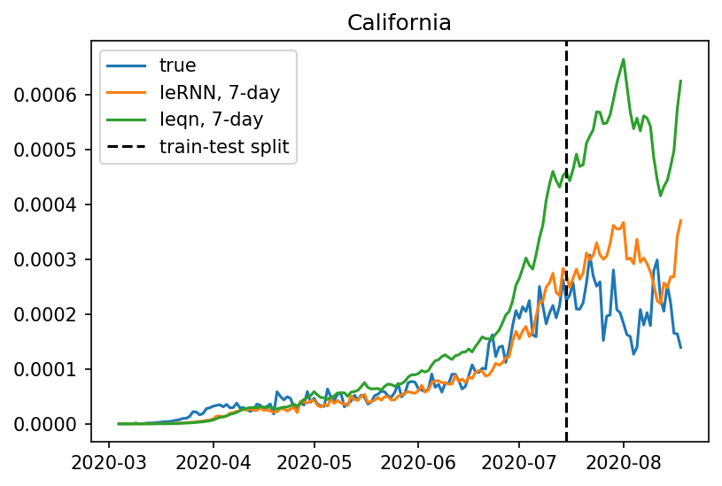
Figure 9: Comparing 7-day ahead predictions of IeRNN and I-equation with training (testing) period to the left (right) of the vertical dashed line. The vertical axis is fraction of newly infected people in the population. The horizontal axis is time in unit of days.

Conclusions

We develop a novel spatio-temporal infectious disease model called IeRNN, which is a hybrid model consisting of I-equation from SEIR driven by spatial features. With such features and RNN dynamics as external input to the I-equation, the robustness to parameter initialization in model training is greatly improved. In 1-day and 7-day ahead prediction, our model outperforms standard temporal models. In future work, the social control mechanisms (Albi, Pareschi, and Zanella 2020; Morris et al. 2020) could be considered to strengthen the I-equation, as well as traffic data to expand inflow effect beyond geographic neighbors.

References

- Albi, Pareschi, and Zanella (2020) Albi, G.; Pareschi, L.; and Zanella, M. 2020. Control with uncertain data of socially structured compartmental epidemic models. arXiv preprint arXiv:2004.13067 .
- Anderson and May (1992) Anderson, R.; and May, R. 1992. Infectious Diseases of Humans: Dynamics and Control. Oxford University Press, Oxford.
- Andrew (2005) Andrew, C. 2005. A map of the United States, with state names (and Washington D.C.). URL https://commons.wikimedia.org/wiki/File:Map˙of˙USA˙with˙state˙names.svg.
- Deng et al. (2019) Deng, S.; Wang, S.; Rangwala, H.; Wang, L.; and Ning, Y. 2019. Graph message passing with cross-location attentions for long-term ILI prediction. arXiv preprint arXiv:1912.10202 .
- Dong, Du, and Gardner (2020) Dong, E.; Du, H.; and Gardner, L. 2020. An interactive web-based dashboard to track COVID-19 in real time. Lancet Inf Dis. 20(5):533-534. doi: 10.1016/S1473-3099(20)30120-1 .
- Hethcote (2000) Hethcote, H. W. 2000. The mathematics of infectious diseases. SIAM Review 42: 599 – 653.
- Hochreiter and Schmidhuber (1997) Hochreiter, S.; and Schmidhuber, J. 1997. Long short-term memory. Neural computation 9(8): 1735–1780.
- Kingma and Ba (2015) Kingma, D.; and Ba, J. 2015. Adam: A Method for Stochastic Optimization. 3rd International Conference for Learning Representations, San Diego, 2015 .
- Lai et al. (2017) Lai, G.; Chang, W.; Yang, Y.; and Liu, H. 2017. Modeling Long- and Short-Term Temporal Patterns with Deep Neural Networks. CoRR abs/1703.07015. URL http://arxiv.org/abs/1703.07015.
- Li et al. (2020) Li, M. L.; Tazi Bouardi, H.; Skali Lami, O.; Trikalinos, T. A.; Trichakis, N. K.; and Bertsimas, D. 2020. Forecasting COVID-19 and Analyzing the Effect of Government Interventions. medRxiv doi:10.1101/2020.06.23.20138693. URL https://www.medrxiv.org/content/early/2020/06/24/2020.06.23.20138693.
- Li et al. (2019) Li, Z.; Luo, X.; Wang, B.; Bertozzi, A.; and Xin, J. 2019. A Study on Graph-Structured Recurrent Neural Networks and Sparsification with Application to Epidemic Forecasting. In World Congress on Global Optimization, 730–739. Springer.
- Morris et al. (2020) Morris, D. H.; Rossine, F. W.; Plotkin, J. B.; and Levin, S. A. 2020. Optimal, near-optimal, and robust epidemic control. arXiv preprint arXiv:2004.02209 .
- Roosa et al. (2020) Roosa, K.; Lee, Y.; Luo, R.; Kirpich, A.; Rothenberg, R.; Hyman, J.; Yan, P.; and Chowell, G. 2020. Real-time forecasts of the COVID-19 epidemic in China from February 5th to February 24th, 2020. Infectious Disease Modelling 5: 256 – 263.
- Wang et al. (2018) Wang, B.; Luo, X.; Zhang, F.; Yuan, B.; Bertozzi, A.; and Brantingham, P. 2018. Graph-based deep modeling and real time forecasting of sparse spatio-temporal data. MiLeTS ’18, London, UK, DOI: 10.475/123_4; arXiv preprint arXiv:1804.00684 .
- Wang et al. (2019) Wang, B.; Yin, P.; Bertozzi, A.; Brantingham, P.; Osher, S.; and Xin, J. 2019. Deep learning for real-time crime forecasting and its ternarization. Chinese Annals of Mathematics, Series B 40(6): 949–966.
- World-Population-Review (2020) World-Population-Review. 2020. US States Population 2020. URL https://worldpopulationreview.com/states.
- Wu et al. (2018) Wu, Y.; Yang, Y.; Nishiura, H.; and Saitoh, M. 2018. Deep Learning for Epidemiological Predictions. The 41st International ACM SIGIR Conference on Research & Development in Information Retrieval .
- Yang, Santillana, and Kou (2015) Yang, S.; Santillana, M.; and Kou, S. 2015. Accurate estimation of influenza epidemics using Google search data via ARGO. Proceedings of the National Academy of Sciences 112(47): 14473–14478.