Catalytic transformations with finite-size environments: applications to cooling and thermometry

Abstract

The laws of thermodynamics are usually formulated under the assumption of infinitely large environments. While this idealization facilitates theoretical treatments, real physical systems are always finite and their interaction range is limited. These constraints have consequences for important tasks such as cooling, not directly captured by the second law of thermodynamics. Here, we study catalytic transformations that cannot be achieved when a system exclusively interacts with a finite environment. Our core result consists of constructive conditions for these transformations, which include the corresponding global unitary operation and the explicit states of all the systems involved. From this result we present various findings regarding the use of catalysts for cooling. First, we show that catalytic cooling is always possible if the dimension of the catalyst is sufficiently large. In particular, the cooling of a qubit using a hot qubit can be maximized with a catalyst as small as a three-level system. We also identify catalytic enhancements for tasks whose implementation is possible without a catalyst. For example, we find that in a multiqubit setup catalytic cooling based on a three-body interaction outperforms standard (non-catalytic) cooling using higher order interactions. Another advantage is illustrated in a thermometry scenario, where a qubit is employed to probe the temperature of the environment. In this case, we show that a catalyst allows to surpass the optimal temperature estimation attained only with the probe.

1 Introduction

In the field of Chemistry, catalysts are substances that can be used to assist a chemical reaction without being consumed in the process. This simple but powerful principle has also found applications in areas of quantum information [1, 2, 3, 4, 5, 6, 7, 8, 9, 10, 11, 12, 13, 14] and quantum thermodynamics [15, 16, 17, 18, 19, 20, 21, 22, 23, 24], where catalysts are quantum systems that enable the implementation of otherwise impossible transformations. For example, transformations that are forbidden under local operations and classical communication (LOCC) become possible once a suitable entangled state is employed as catalyst [1]. Regarding the technical aspect, catalytic transformations have often been addressed using the concept of “catalytic majorization” [2, 3, 4] and related extensions [19, 25]. A distinctive feature of this approach is that it provides general conditions for the existence of a catalyst state that enables the transformation. However, typically such a state and the corresponding implementation are not explicitly given.

In quantum thermodynamics, it has been shown that catalysts extend the set of state transitions that a system can undergo in the presence of a thermal environment [15, 19]. These transformations are performed through global unitaries that couple the environment with the rest of the system, and preserve the energy of the total setup. Originally introduced without the inclusion of catalysts, such conditions define maps on the system known as “thermal operations” [26, 27, 28, 29, 30, 31, 32, 33]. Although a few studies have addressed thermal operations with finite environments [30, 34, 35], the most general transformations derived within this framework rely on the possibility of interactions with arbitrarily large baths (determined by arbitrary bath Hamiltonians)[26, 31] — an assumption that has also been adopted in the case of catalytic thermal operations [15, 18, 19, 20, 24]. Here, we consider catalytic transformations where the main system interacts with a catalyst and a finite environment. The transformations result from the application of non-energy preserving unitaries on the total system, and the enviroment may start in a generic state. Moreover, they are explicit, in the sense that explicit unitaries and the corresponding catalyst state are obtained. From a thermodynamic viewpoint, the main motivation is the characterization of conditions to catalytically circumvent cooling limitations due to the finite character of the environment.

The interest in the formalization and quantification of the fundamental limits for cooling has seen a resurgence in the last years [36, 37]. One approach is to cast these limits as bounds on the duration of continuous [38, 39] or discrete cooling processes [30, 40, 41], in the spirit of the celebrated unattainability principle [36, 42]. Alternatively, bounds for maximum cooling have been derived for different kinds of refrigerators operating in the steady-state regime [43] and heat bath algorithmic cooling protocols [44, 45]. In principle, the saturability of these bounds requires an infinite amount of time (or an infinite number of discrete steps), and therefore time emerges as a fundamental resource in this context.

Naturally, the maximum degree of cooling depends not only on the available time but also on other physical resources [36, 46, 47, 48]. In addition to standard thermodynamic resources such as work and heat, other factors that have been proven useful for assisting cooling are the access to non-equilibrium states [18], in the framework of catalytic thermal operations, the (Hilbert space) dimension of microscopic refrigerators [49, 50], and quantum properties such as coherence [51] and entanglement [52]. In contrast, we are interested in a limiting factor that can dramatically restrict the ability to cool. Namely, the limited access to the environment where heat is dissipated. Although this issue has been addressed in previous studies [35, 53, 54, 55, 56], we consider extreme cases where cooling is not even possible. For example, if the environment is very small and very hot [57]. After introducing some notational conventions, this limitation is illustrated with a simple and intuitive example in Sect. II. Using the notion of passivity [58, 59, 60, 61], we characterize the impossibility to cool using a small environment in Sect. III. Next, we establish sufficient conditions to lift this restriction in Sect. IV (Corollary 1), by means of a finite-dimensional and single-copy catalyst. In the same section we also present a graphical method that provides an intuitive picture of the studied catalytic transformations.

On the technical side, the results of Sect. IV are applicable to a broader class of catalytic transformations, which we dub “non-unital transformations” (Definition 3). These transformations are characterized in Corollary 2 and include cooling as a particular case. Moreover, we show that two established results on catalysts fall within this general class: catalytic extraction of work from a passive state [17], and a catalytic violation of the Jarzynski fluctuation theorem [22].

In Sect. V, we present a theorem (Theorem 2) where the dimension of the catalyst is shown to play a key role for both cooling and non-unital transformations in general. This theorem states that such transformations can be implemented for almost any initial state of the system and the environment, if the catalyst dimension is sufficiently large. These findings are illustrated in Sect. VI through several examples. First, we consider the task of optimizing the cooling of a two-level system using another two-level system as environment, and catalysts of different dimensions. On the one hand, it is shown that the catalyst dimension required to bypass the passivity constraint increases as the system approaches its ground state, given a fixed state of the environment. If the system state and the environment state are close to each other, we instead see that the smallest catalyst (i.e. another two-level system) suffices to cool. Next, we show that it is also possible to catalytically increase the ground population of the system, which is yet another example of non-unital transformation. Section VI is concluded by showing that, in cases where cooling is possible without a catalyst, a sufficiently large catalyst provides a cooling enhancement. We present a general statement of this advantage, for the cooling of a two-level system using an environment of even dimension (Theorem 3). In the case of odd dimension, we illustrate a cooling enhancement through a two-level catalyst, after maximum cooling of a qubit has been performed using a three-level environment.

Sections VII and VIII are also framed within the context of catalytic enhancements. In Sect. VII we address the problem of cooling a group of qubits, using environments composed of different numbers of identical qubits. We find that the introduction of a two-level catalyst can provide a two-fold advantage. First, if the environment is not too large compared to the number of cooled qubits, the catalyst allows to extract more heat. Secondly, cooling without the catalyst requires potentially much more complex interactions. In Sect. VIII we illustrate an application to thermometry [62]. Thermometry makes part of the broader field of metrology [63, 64, 65, 66] and aims at estimating the temperature of some environment at thermal equilibrium. In particular, temperature information can be transferred to a probe that undergoes a suitable coupling with the environment [67, 68, 69, 70, 71, 72, 73, 74, 75, 76, 77]. We show that this information can be increased via a two-level catalyst, thereby reducing the error in the temperature estimation. Finally, we present the conclusions and outlook in Sect. IX.

2 Preliminaries

Henceforth we will often call the system to be cooled and the environment “cold object” and “hot object”, respectively. Moreover, the ground state of these systems and the catalyst will be denoted using the label “1” instead of ”0”. This choice is convenient to simplify the notation of other physical quantities that will be defined later. States that describe the total system (formed by the catalyst, the cold object and the hot object) are written without labels, as well as the corresponding unitary operations. This also simplifies notation and does not generate ambiguity, since this is the only three-partite setup considered.

The eigendecompositions of local states read

$$\rho_{x}=\sum_{i=1}^{d_{x}}p_{i}^{x}|i_{x}\rangle\langle i_{x}|,$$ (1)

where the label $x$ can refer to the cold object ($x=c$), the hot object ($x=h$), or the catalyst ($x=v$). Moreover, $d_{x}$ stands for the dimension of the corresponding Hilbert space $\mathcal{H}_{x}$. We also adopt a convention of non-increasing eigenvalues, $p_{i}^{x}\geq p_{i+1}^{x}$ for all $1\leq i\leq d_{x}$, which is useful for the description of passive states.

Figure 1: Framework for catalytic and cooling transformations. (a) Illustrative example: a three-level system in the initial state $\rho_{h}$ is used as hot object to cool a (cold) qubit in the initial state $\rho_{c}$. The eigenvalues of the joint state $\rho_{ch}=\rho_{c}\otimes\rho_{h}$ are obtained by rescaling the eigenvalues of $\rho_{h}$ (orange bars) with the eigenvalues of $\rho_{c}$. If $p_{2}^{c}p_{1}^{h}>p_{1}^{c}p_{3}^{h}$ cooling is possible by swapping (black arrows) the eigenstates $|1_{c}3_{h}\rangle$ and $|2_{c}1_{h}\rangle$. If $\rho_{c}$ and $\rho_{h}$ are thermal states with respective temperatures $T_{c}$ and $T_{h}$, and $T_{h}$ is too high or $T_{c}$ is too low, no unitary $U_{ch}$ applied on $\rho_{ch}$ can perform cooling. (b) This restriction can be bypassed through a global unitary $U$ applied on $\rho=\rho_{ch}\otimes\rho_{v}$, where $\rho_{v}$ is an appropriate catalyst state, and correlations are allowed in the final state $\rho^{\prime}$. (c) In our scheme cooling is first implemented through a “cooling unitary” $U_{\textrm{cool}}$, which perturbs the catalyst, and followed by a unitary $V_{\textrm{res}}$ that brings it back to $\rho_{v}$. Hence, we assume the form $U=V_{\textrm{res}}U_{\textrm{cool}}$.

Although most of the time we will be dealing with an initial uncorrelated state $\rho=\rho_{c}\otimes\rho_{h}\otimes\rho_{v}$, some times we will refer to the joint state of the cold and hot objects as $\rho_{ch}$. In such a case, it must be understood that $\rho_{ch}$ is a general state, unless we explicitly write $\rho_{ch}=\rho_{c}\otimes\rho_{h}$. The general eigendecomposition for $\rho_{ch}$ (including the special case $\rho_{c}\otimes\rho_{h}$) is written as $\rho_{ch}=\sum_{\psi=1}^{d_{c}d_{h}}p_{\psi}^{ch}|\psi_{ch}\rangle\langle\psi_{ch}|$, with non-increasing eigenvalues $p_{\psi}^{ch}\geq p_{\psi+1}^{ch}$. The greek letters $\psi$ and $\varphi$ will also be used as indices for the eigendecomposition of $\rho$. For example, $\rho=\sum_{\psi}p_{\psi}|\psi\rangle\langle\psi|$, with the absence of the label “$ch$” distinguishing its eigenstates from those of $\rho_{ch}$. For product states $\rho_{c}\otimes\rho_{h}\otimes\rho_{v}$ the global eigenstates are also denoted as $|i_{c}j_{h}k_{v}\rangle=|i_{c}\rangle\otimes|j_{h}\rangle\otimes|k_{v}\rangle$.

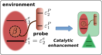
Figure 1(a) illustrates a situation where cooling with a very small hot object is forbidden. Here, the cold object is a qubit in the initial state $\rho_{c}=\sum_{i=1}^{2}p_{i}^{c}|i_{c}\rangle\langle i_{c}|$, and the hot object is a three-level system in the state $\rho_{h}=\sum_{j=1}^{3}p_{j}^{c}|j_{h}\rangle\langle j_{h}|$. With the prescription of non-increasing eigenvalues, cooling is possible if and only if $p_{1}^{c}p_{3}^{h}<p_{2}^{c}p_{1}^{h}$. The case $p_{1}^{c}p_{3}^{h}\geq p_{2}^{c}p_{1}^{h}$ constitutes an example of passivity in the context of cooling, characterized for generic systems (with discrete Hamiltonians) in the next section (cf. Eq. (3)). As explained in Sect. IV, such a cooling limitation can be circumvented by adding a catalyst in a proper initial state $\rho_{v}$, such that it allows cooling and also remains unaltered by the transformation. The action of the studied catalytic transformations on the compound of hot and cold objects is illustrated in Fig. 1(b). In particular, the generation of correlations between the catalyst and the rest of the total system is allowed. This condition is characteristic of recent works on catalysts [17, 19, 24] and is also natural in our framework, where all the systems involved can be arbitrarily small. A more detailed form of the global unitaries that implement the transformations is shown in Fig. 1(c).

3 Passivity and cooling

The fundamental limits for cooling can be understood using the notion of passivity. Passivity is essentially a condition whereby applying unitary transformations to a system cannot decrease the mean value of certain observables. While traditionally it has been associated with the Hamiltonian and the impossibility of work extraction [59, 78, 79, 80, 81], passivity can be extended to any hermitian operator that represents an observable [57, 61].

Since we will also be dealing with passive states of the cold object in the traditional sense, it is important to characterize them before introducing our extended definition, directly related to the task of cooling. A state $\rho_{c}$ is called passive if and only if its average energy cannot be decreased using local unitary evolutions $U_{c}$ [59]. That is, if $\Delta\bigl{\langle}H_{c}\bigr{\rangle}=\textrm{Tr}\left[H_{c}\left(U_{c}\rho_{c}U_{c}^{\dagger}-\rho_{c}\right)\right]\geq 0$ for any $U_{c}$. In quantum thermodynamics, this means that it is impossible to extract work from $\rho_{c}$ via any classical driving. Importantly, any thermal state is passive but there are many passive states that are non-thermal. Specifically, $\rho_{c}$ is passive if and only if $[\rho_{c},H_{c}]=0$ and the eigenvalues of $\rho_{c}$ are non-increasing with respect to the eigenenergies of $H_{c}$. Assuming the sorting $p_{i}^{c}\geq p_{i+1}^{c}$, we have that $\rho_{c}$ is passive iff $H_{c}=\sum_{i}\varepsilon_{i}^{c}|i_{c}\rangle\langle i_{c}|$, and $\varepsilon_{i+1}^{c}\geq\varepsilon_{i}^{c}$.

3.1 Passive states for cooling

Consider now a bipartite system in the initial state $\rho_{c}\otimes\rho_{h}$, where $\rho_{c}$ is a passive state. Since local unitaries on $\rho_{c}$ cannot decrease its average energy, we wonder if global unitaries $U_{ch}$ on the compound $\rho_{c}\otimes\rho_{h}$ can do so. We say that $\rho_{c}\otimes\rho_{h}$ is passive with respect to $H_{c}$, iff

$$\Delta\bigl{\langle}H_{c}\bigr{\rangle}\geq 0\textrm{ for any }U_{ch},$$ (2)

where $\Delta\bigl{\langle}H_{c}\bigr{\rangle}=\textrm{Tr}\left[H_{c}\left(U_{ch}\rho_{c}\otimes\rho_{h}U_{ch}^{\dagger}-\rho_{c}\otimes\rho_{h}\right)\right]$. Conversely, if $\Delta\left\langle H_{c}\right\rangle<0$ for some $U_{ch}$, then $\rho_{c}\otimes\rho_{h}$ is non-passive with respect to $H_{c}$.

In Appendix A we characterize the conditions for passivity of any state $\rho_{c}\otimes\rho_{h}$ in terms of its eigenvalues. We find that $\rho_{c}\otimes\rho_{h}$ is also passive with respect to $H_{c}$ iff the following inequalites hold:

$$\frac{p_{i}^{c}}{p_{i+1}^{c}}\geq\frac{p_{1}^{h}}{p_{d_{h}}^{h}}\textrm{ for all }i.$$ (3)

We remark that Eq. (3) is obtained without assuming anything on the Hamiltonian of the hot object or the eigenstates of $\rho_{h}$. Interestingly, this expression tells us that the only relevant parameter behind passivity is the ratio between the highest and smallest eigenvalues of the hot object [82]. In particular, it allows us to understand why a thermal state $\rho_{h}$ at a very high temperature $T_{h}$ can prevent cooling. If $\{\varepsilon_{j}^{h}\}_{j=1}^{d_{h}}$ denotes the energy spectrum of the hot object, the ratio $p_{1}^{h}/p_{d_{h}}^{h}$ reads $p_{1}^{h}/p_{d_{h}}^{h}=e^{(\varepsilon_{d_{h}}^{h}-\varepsilon_{1}^{h})/T_{h}}$. In the limit $\varepsilon_{d_{h}}^{h}-\varepsilon_{1}^{h}\ll T_{h}$, this ratio tends to one and consequently all the inequalities (3) are satisfied (keeping in mind the convention $p_{i}^{c}\geq p_{i+1}^{c}$). Similarly, for a thermal state $\rho_{c}$ the ratios $p_{i}^{c}/p_{i+1}^{c}$ become larger the lower the corresponding temperature, making more feasible the scenario (3).

3.2 Remarks on cooling

Traditionally, the task of cooling is defined as a heat exchange between two systems at thermal equilibrium, where heat is extracted from the system at lower temperature. In this paper we will adopt a more general approach, whose main requirement is the passivity of the state $\rho_{c}$. In this view the only Hamiltonian that plays a relevant role is that of the cold object, and the only energetic transformation that we care about is the reduction of the average energy $\bigl{\langle}H_{c}\bigr{\rangle}$. Due to the passive character of $\rho_{c}$, cooling is only possible by attaching an ancillary system to the cold object and performing a global unitary evolution on the resulting compound. This ancillary system can be the hot object alone (if $\rho_{c}\otimes\rho_{h}$ is non-passive), or the hot object in combination with a catalyst.

It is important to note that cooling is also typically associated with a work investment, according to the second law of thermodynamics. Another manifestation of this energetic cost is the heat dissipated into the environment, which should be larger than the extracted heat if the environment is equilibrated at a higher temperature. Since we do not need to specify the Hamiltonian of the hot object (recall that the hot object and the environment represent the same system), neither to assume that it starts in a thermal state, predictions on its energetic behavior are irrelevant for our analysis. Essentially, its role is restricted to mediate the reduction of the average energy $\bigl{\langle}H_{c}\bigr{\rangle}$. That being said, we also stress this scenario coincides with the traditional characterization of cooling, if $\rho_{c}$ and $\rho_{h}$ are both thermal states and their temperatures satisfy $T_{c}\leq T_{h}$.

4 Catalytic transformations

4.1 Catalytic transformations and cooling

Given the passivity condition (3), our goal is to introduce a third system that enables cooling and works as a catalyst. This means that if the catalyst is initially in a state $\rho_{v}=\sum_{k=1}^{d_{v}}p_{k}^{v}|k_{v}\rangle\langle k_{v}|$, at the end of the transformation it must be returned to the same state. In addition, we assume that the catalyst starts uncorrelated from the cold and objects, i.e. the initial total state is $\rho=\rho_{c}\otimes\rho_{h}\otimes\rho_{v}$. The transformation on the cold object is implemented through a global unitary map $U$ that acts on the total system. Denoting the final total state as $\rho^{\prime}$, a generic catalytic transformation satisfies

$$\rho\rightarrow\rho^{\prime} =U(\rho_{c}\otimes\rho_{h}\otimes\rho_{v})U^{\dagger},$$ (4)

$$\textrm{Tr}_{ch}(\rho^{\prime}) =\rho_{v}.$$ (5)

Note that Eq. (5) guarantees “catalysis” (i.e. the restoration of the catalyst to its initial state) but does not say anything about the final correlations between the catalyst and the rest of the total system. Allowing correlations has proven to be useful in extending the transformations that a system can undergo in the presence of a catalyst [17, 19, 22, 23, 24]. In addition to this possibility, the repeated implementation of a given transformation is naturally associated with the notion of catalyst. For example, under the condition (5) the transformation (4) can be performed as many times as desired, using the same catalyst, and provided that each transformation involves a new copy of the state $\rho_{c}\otimes\rho_{h}$. This property will be of special importance for the results presented in Sect. VII.

4.1.1 Cooling and catalyst restoration

Given a passive state $\rho_{c}\otimes\rho_{h}$, the catalyst allows to reduce the mean energy $\left\langle H_{c}\right\rangle$ as long as the total state $\rho_{c}\otimes\rho_{h}\otimes\rho_{v}$ is non-passive with respect to $H_{c}$. The verification of this condition is simple but a bit subtle. Specifically, we can straightforwardly apply the characterization of passivity (3) to $\rho_{c}\otimes\rho_{h}\otimes\rho_{v}$, by considering $\rho_{h}\otimes\rho_{v}$ as the state of a new “effective” hot object. This amounts to replace $p_{1}^{h}$ and $p_{d_{h}}^{h}$ by the largest and minimum eigenvalues of $\rho_{h}\otimes\rho_{v}$, which are respectively given by $p_{1}^{h}p_{1}^{v}$ and $p_{d_{h}}^{h}p_{d_{v}}^{v}$. In this way, the catalyst allows to break down the passivity constraint if and only if there exists $i^{\prime}$ such that

$$\frac{p_{i^{\prime}}^{c}}{p_{i^{\prime}+1}^{c}}<\frac{p_{1}^{h}p_{1}^{v}}{p_{d_{h}}^{h}p_{d_{v}}^{v}}.$$ (6)

Since the ratio at the r.h.s. of Eq. (6) is always larger than $p_{1}^{h}/p_{d_{h}}^{h}$, by a factor of $p_{1}^{v}/p_{d_{v}}^{v}$, passivity with respect to $\rho_{c}\otimes\rho_{h}\otimes\rho_{v}$ can be violated, even if all the inequalities (3) are satisfied. In particular, a divergent ratio results if $\rho_{v}=|1_{v}\rangle\langle 1_{v}|$. However, we will see later that the catalysis condition (5) requires the use of catalysts in initial mixed states.

Once Eq. (6) is satisfied, $\rho$ is a non-passive state and cooling is possible by applying a global unitary. For example, consider the unitary $\mathcal{U}_{|i^{\prime}_{c}d_{h}d_{v}\rangle\leftrightarrow|(i^{\prime}+1)_{c}1_{h}1_{v}\rangle}$, which swaps the eigenstates $|i^{\prime}_{c}d_{h}d_{v}\rangle$ and $|(i^{\prime}+1)_{c}1_{h}1_{v}\rangle$ and acts as the identity on any other eigenstate of $\rho$. That is,

$$\mathcal{U}_{|i^{\prime}_{c}d_{h}d_{v}\rangle\leftrightarrow|(i^{\prime}+1)_{c}1_{h}1_{v}\rangle}|i^{\prime}_{c}d_{h}d_{v}\rangle =|(i^{\prime}+1)_{c}1_{h}1_{v}\rangle,$$

$$\mathcal{U}_{|i^{\prime}_{c}d_{h}d_{v}\rangle\leftrightarrow|(i^{\prime}+1)_{c}1_{h}1_{v}\rangle}|(i^{\prime}+1)_{c}1_{h}1_{v}\rangle =|i^{\prime}_{c}d_{h}d_{v}\rangle.$$ (7)

When applied on $\rho$, Eq. (7) yields a state where the only effect is to exchange the eigenvalues of $|i^{\prime}_{c}d_{h}d_{v}\rangle$ and $|(i^{\prime}+1)_{c}1_{h}1_{v}\rangle$. In this way, (6) implies that

$$\Delta\bigl{\langle}H_{c}\bigr{\rangle}=\left(p_{i^{\prime}}^{c}p_{d_{h}}^{h}p_{d_{v}}^{v}-p_{i^{\prime}+1}^{c}p_{1}^{h}p_{1}^{v}\right)(\varepsilon_{i^{\prime}+1}^{c}-\varepsilon_{i^{\prime}}^{c})<0.$$ (8)

However, the swap in Eqs. (7) also modifies the initial state of the catalyst. Denoting as $\bigl{\langle}|k_{v}\rangle\langle k_{v}|\bigr{\rangle}=\textrm{Tr}\left[|k_{v}\rangle\langle k_{v}|\rho\right]$ the catalyst population corresponding to the eigenstate $|k_{v}\rangle$, it increases $\bigl{\langle}|d_{v}\rangle\langle d_{v}|\bigr{\rangle}$ by $p_{i^{\prime}}^{c}p_{d_{h}}^{h}p_{d_{v}}^{v}-p_{i^{\prime}+1}^{c}p_{1}^{h}p_{1}^{v}$ and reduces $\bigl{\langle}|1_{v}\rangle\langle 1_{v}|\bigr{\rangle}$ by the same amount. This example motivates the introduction of the following definitions, which are crucial for our analysis of catalytic and cooling transformations. In these definitions an initial state of the standard form $\rho=\rho_{c}\otimes\rho_{h}\otimes\rho_{v}$ is assumed.

Definition 1 (Cooling unitary). A cooling unitary, denoted as $U_{\textrm{cool}}$, is a unitary that satisfies $\textrm{Tr}(H_{c}U_{\textrm{cool}}\rho U_{\textrm{cool}}^{\dagger})<\textrm{Tr}(H_{c}\rho)$. An example of cooling unitary is the swap described in Eqs. (7).

Definition 2 (Restoring unitary). Given an initial transformation $\rho\rightarrow\sigma$ that modifies the catalyst state (i.e. $\textrm{Tr}_{ch}(\sigma)\neq\rho_{v}$), a restoring unitary $V_{\textrm{res}}$ is a unitary that satisfies $\textrm{Tr}_{ch}(V_{\textrm{res}}\sigma V_{\textrm{res}}^{\dagger})=\rho_{v}$.

4.1.2 Unitary operations involved in catalytic transformations

Henceforth, any unitary that restores the catalyst or contributes to its restoration will be denoted using the symbol $V$, instead of $U$. However, the following remarks and any subsequent comment regarding a general unitary $U$ are also valid for $V$.

Given a unitary $U$ and a Hilbert subspace $\mathcal{H}_{\textrm{sub}}\subseteq\mathcal{H}$, being $\mathcal{H}_{\textrm{sub}}$ spanned by a subset of eigenstates of $\rho$, we say that $U$ maps $\mathcal{H}_{\textrm{sub}}$ into itself if:

1. $U|\psi\rangle=|\psi\rangle$ for $|\psi\rangle\notin\mathcal{H}_{\textrm{sub}}$.

2. $U|\psi\rangle\in\mathcal{H}_{\textrm{sub}}$ for $|\psi\rangle\in\mathcal{H}_{\textrm{sub}}$.

Equivalently, if $U$ satisfies conditions 1 and 2 we also say that “$U$ acts on $\mathcal{H}_{\textrm{sub}}$” , which is symbolically written as $U:\mathcal{H}_{\textrm{sub}}\rightarrow\mathcal{H}_{\textrm{sub}}$.

Our interest will be on transformations of the form $\rho\rightarrow\rho^{\prime}=U\rho U^{\dagger}$, where

$$U=V_{\textrm{res}}U_{\textrm{cool}}.$$ (9)

Following Definition 2, these transformations are catalytic by construction, since $V_{\textrm{res}}$ restores the catalyst state initially modified by the transformation $\rho\rightarrow\sigma=U_{\textrm{cool}}\rho U_{\textrm{cool}}^{\dagger}$.

While there may exist many cooling unitaries if $\rho$ is non-passive, we will focus on the most basic unitary that allows cooling and admits a “simple” solution to the problem of catalyst restoration. Namely, a cooling unitary that acts on a two-dimensional subspace $\mathcal{H}_{\textrm{sub}}$, which we term “two-level unitary”. The swap (7) is an example of such an operation. Under the transformation $\rho\rightarrow\sigma$ implemented by this swap, it would be necessary to find a restoring unitary that recovers the populations $\bigl{\langle}|1_{v}\rangle\langle 1_{v}|\bigr{\rangle}$ and $\bigl{\langle}|d_{v}\rangle\langle d_{v}|\bigr{\rangle}$. In some situations this may not be possible, and therefore it is convenient to explore other two-level unitaries whose effect can be reverted via a suitable $V_{\textrm{res}}$. This leads us to present an alternative formulation of Eq. (6). Using such a formulation, we will be able to broaden the possibilities for catalyst restoration, by finding a variety of two-level cooling unitaries that have different effects on the catalyst.

Specifically, the inequality (6) can be rewritten in the equivalent way:

$$\frac{p_{i^{\prime}}^{c}}{p_{i^{\prime}+1}^{c}}<\frac{p_{1}^{h}p_{l}^{v}}{p_{d_{h}}^{h}p_{l^{\prime}+1}^{v}},$$ (10)

for some set of indices $\{i^{\prime},l,l^{\prime}\}$ such that $i^{\prime}\in\{1,2,...,d_{c}-1\}$ and $l,l^{\prime}\in\{1,2,...,d_{v}-1\}$. Equation (6) implies Eq. (10), because $\{i^{\prime},l,l^{\prime}\}=\{i^{\prime},1,d_{v}-1\}$ is an example of such a set of indices. Conversely, since $\frac{p_{1}^{h}p_{l}^{v}}{p_{d_{h}}^{h}p_{l^{\prime}+1}^{v}}\leq\frac{p_{1}^{h}p_{1}^{v}}{p_{d_{h}}^{h}p_{d_{v}}^{v}}$, the inequality (10) implies Eq. (6).

In Sect. IV-B2 we will apply Eq. (10) to identify a familiy of two-level cooling unitaries and the corresponding restoring unitaries. These restoring unitaries act on a subspace

$$\mathcal{H}_{n,N}\equiv\textrm{span}\{|\psi_{ch}\rangle\}_{\psi=n}^{N}\otimes\mathcal{H}_{v},$$ (11)

where $n$ and $N$ are two numbers such that $n\leq N-1$ and $n,N\in\{1,2,...,d_{c}d_{h}\}$. We remark that the eigenstates in the set $\{|\psi_{ch}\rangle\}_{\psi=n}^{N}$ are arranged according to the sorting $p_{\psi}^{ch}\geq p_{\psi+1}^{ch}$. For example, $|1_{ch}\rangle$ possess the largest eigenvalue $p_{1}^{ch}=p_{1}^{h}p_{1}^{c}$, and therefore it is the “first” eigenstate of $\rho_{c}\otimes\rho_{h}$. This observation is also important to understand that the eigenstates $|n_{ch}\rangle$ and $|N_{ch}\rangle$ in Eqs. (24) and (27) are consistent with the condition $p_{n}^{ch}\geq p_{N}^{ch}$.

4.2 Catalytic transformations and population currents

The effect of the swap $\mathcal{U}_{|i^{\prime}_{c}d_{h}d_{v}\rangle\leftrightarrow|(i^{\prime}+1)_{c}1_{h}1_{v}\rangle}$ can be more conveniently described as a population transfer from the eigenstate $|1_{v}\rangle$ towards the eigenstate $|d_{v}\rangle$, since the increment in $\left\langle|d_{v}\rangle\langle d_{v}|\right\rangle$ equals exactly the reduction in $\left\langle|1_{v}\rangle\langle 1_{v}|\right\rangle$. That is, $\Delta\left\langle|d_{v}\rangle\langle d_{v}|\right\rangle=-\Delta\left\langle|1_{v}\rangle\langle 1_{v}|\right\rangle$. In this way, a possible restoring unitary would be a two-level unitary that transfers the same population in the opposite direction, i.e. from $|d_{v}\rangle$ to $|1_{v}\rangle$. If the final state of the catalyst is also diagonal in the eigenbasis $\{|k_{v}\rangle\}_{k}$, such an operation is sufficient for its full recovery. Note also that this could be trivially achieved with $V_{\textrm{res}}=\mathcal{U}_{|i^{\prime}_{c}d_{h}d_{v}\rangle\leftrightarrow|(i^{\prime}+1)_{c}1_{h}1_{v}\rangle}^{\dagger}$. However, we are obviously interested in a recovery operation that does not cancel the effect of the cooling unitary on the cold object.

In general, it is not possible to perform a complete catalyst restoration via a single two-level unitary. Notwithstanding, a composition of many two-level unitaries can operate jointly towards the realization of this goal. As an extension of the compensation between population transfers mentioned before, the restoration mechanism in this case can be understood as the result of a series of population transfers that cancel each other. These population transfers are an example of what we call “local currents”, since they involve eigenstates of the catalyst. Other forms of local currents refer to population transfers between eigenstates of the cold object, or between eigenstates of the hot object. It is important to stress that this notion of current describes a net population transfer, rather than some rate of population exchanged per unit of time. With this observation in mind, in what follows we introduce the basic tools for the characterization of local currents, by connecting them with population transfers between eigenstates of $\rho$, also termed “global currents”.

4.2.1 Characterization of local and global currents

Let us denote a general two-level as $U^{(2)}$, with the superscript “$(2)$” indicating that it maps a two-dimensional subspace into itself. If $|\psi\rangle$ and $|\varphi\rangle$ are eigenstates of $\rho$ that expand this subspace, $U^{(2)}$ performs a population transfer between $|\psi\rangle$ and $|\varphi\rangle$ that we can fully characterize through the equations

$$U^{(2)}|\psi\rangle =\sqrt{1-r}|\psi\rangle+\sqrt{r}|\varphi\rangle,$$ (12)

$$U^{(2)}|\varphi\rangle =\sqrt{r}|\psi\rangle-\sqrt{1-r}|\varphi\rangle,$$ (13)

where $0\leq r\leq 1$ is the probability that $|\psi\rangle$ and $|\varphi\rangle$ are swapped, or “swap intensity”. For $0\leq r<1$, we say that $U^{(2)}$ is a “partial swap”, and also denote it as $U_{|\psi\rangle\leftrightarrow|\varphi\rangle}$. For $r=1$, the corresponding total swap (or simply “swap”) is denoted as $\mathcal{U}^{(2)}$ or $\mathcal{U}_{|\psi\rangle\leftrightarrow|\varphi\rangle}$. Importantly, the swap intensity is not affected by the addition of local or global phases in Eqs. (12) and (13). Since $r$ is the only parameter we care about, we restrict ourselves (and without loss of generality) to the description of two-level unitaries given by these equations. Note also that the swap intensity is invariant if we exchange $\psi$ and $\varphi$. Hence, both $U_{|\psi\rangle\leftrightarrow|\varphi\rangle}$ and $U_{|\varphi\rangle\leftrightarrow|\psi\rangle}$ are two-level unitaries that swap $|\psi\rangle$ and $|\varphi\rangle$ with probability $r$.

Although $U^{(2)}$ in Eqs. (12) and (13) is defined on (a subspace of) the total Hilbert space $\mathcal{H}$, we remark that the action of two-level unitaries acting on local Hilbert spaces can be analogously formulated. In particular, we will also consider two-level unitaries that act on the Hilbert spaces $\mathcal{H}_{c}\otimes\mathcal{H}_{h}$ and $\mathcal{H}_{c}\otimes\mathcal{H}_{v}$. These maps can be described by simply replacing $|\psi\rangle$ and $|\varphi\rangle$ in (12) and (13) by eigenstates of $\rho_{c}\otimes\rho_{h}$, in the first case, or by eigenstates of $\rho_{c}\otimes\rho_{v}$, in the second case. For example, a two-level unitary $U_{|\psi_{ch}\rangle\leftrightarrow|\varphi_{ch}\rangle}$ swaps the eigenstates $|\psi_{ch}\rangle$ and $|\varphi_{ch}\rangle$ with probability $r$.

For initial populations $p_{\psi}=\textrm{Tr}(|\psi\rangle\langle\psi|\rho)$ and $p_{\varphi}=\textrm{Tr}(|\varphi\rangle\langle\varphi|\rho)$, Eqs. (12) and (13) yield the final population

$$p_{\psi}^{\prime} =\textrm{Tr}[|\psi\rangle\langle\psi|U^{(2)}\rho U^{(2)\dagger}]$$

$$=p_{\psi}+r(p_{\varphi}-p_{\psi}).$$ (14)

We identify the population transfer $\Delta p_{\psi}=p_{\psi}^{\prime}-p_{\psi}$ with a “global current” $J_{|\varphi\rangle\rightarrow|\psi\rangle}=\Delta p_{\psi}$, from the eigenstate $|\varphi\rangle$ towards the eigenstate $|\psi\rangle$. If $J_{|\varphi\rangle\rightarrow|\psi\rangle}$ is negative, it indicates that the transfer takes place in the opposite direction. From Eq. (14) we obtain

$$J_{|\varphi\rangle\rightarrow|\psi\rangle}=r(p_{\varphi}-p_{\psi}).$$ (15)

The maximum population transfer corresponds to a swap $\mathcal{U}_{|\psi\rangle\leftrightarrow|\varphi\rangle}$, and the associated current is denoted as $\mathcal{J}_{|\varphi\rangle\rightarrow|\psi\rangle}$. That is,

$$\mathcal{J}_{|\varphi\rangle\rightarrow|\psi\rangle}=p_{\varphi}-p_{\psi}.$$ (16)

To establish the connection between the global current (15) and local currents let us write the eigenstates $|\psi\rangle$ and $|\varphi\rangle$ as $|\psi\rangle=|i_{c}^{\prime}j_{h}^{\prime}k_{v}^{\prime}\rangle$ and $|\varphi\rangle=|i_{c}^{\prime\prime}j_{h}^{\prime\prime}k_{v}^{\prime\prime}\rangle$. Moreover, let $J_{|k_{v}^{\prime\prime}\rangle\rightarrow|k_{v}^{\prime}\rangle}$ denote the local current from $|k_{v}^{\prime\prime}\rangle$ to $|k_{v}^{\prime}\rangle$, and let us denote the currents from $|i_{c}^{\prime\prime}\rangle$ to $|i_{c}^{\prime}\rangle$ and from $|j_{h}^{\prime\prime}\rangle$ to $|j_{h}^{\prime}\rangle$ as $J_{|i_{c}^{\prime\prime}\rangle\rightarrow|i_{c}^{\prime}\rangle}$ and $J_{|j_{h}^{\prime\prime}\rangle\rightarrow|j_{h}^{\prime}\rangle}$, respectively. In Appendix C2, we apply Eqs. (12) and (13) to show that

$$J_{|i_{c}^{\prime\prime}\rangle\rightarrow|i_{c}^{\prime}\rangle} =r\mathcal{J}_{|\varphi\rangle\rightarrow|\psi\rangle}\leq\left|\mathcal{J}_{|i_{c}^{\prime\prime}\rangle\rightarrow|i_{c}^{\prime}\rangle}\right|,$$ (17)

$$J_{|j_{h}^{\prime\prime}\rangle\rightarrow|j_{h}^{\prime}\rangle} =r\mathcal{J}_{|\varphi\rangle\rightarrow|\psi\rangle}\leq\left|\mathcal{J}_{|j_{h}^{\prime\prime}\rangle\rightarrow|j_{h}^{\prime}\rangle}\right|,$$ (18)

$$J_{|k_{v}^{\prime\prime}\rangle\rightarrow|k_{v}^{\prime}\rangle} =r\mathcal{J}_{|\varphi\rangle\rightarrow|\psi\rangle}\leq\left|\mathcal{J}_{|k_{v}^{\prime\prime}\rangle\rightarrow|k_{v}^{\prime}\rangle}\right|,$$ (19)

where the equalities imply that the local currents coincide with $J_{|\varphi\rangle\rightarrow|\psi\rangle}$ (cf. Eqs. (15) and (16)). In addition, each bound is the absolute value of the local current obtained by applying the swap $\mathcal{U}_{|\psi\rangle\leftrightarrow|\varphi\rangle}$.

4.2.2 Two important classes of catalytic transformations

In combination with Eqs. (15), (16) and (17), we can now apply Eq. (10) to show that the non-passivity of $\rho$ is tantamount to the existence of a two-level cooling unitary characterized below. Specifically, consider the unitary

$$U_{i^{\prime},l,l^{\prime}}\equiv U_{|i_{c}^{\prime}d_{h}(l^{\prime}+1)_{v}\rangle\leftrightarrow|(i^{\prime}+1)_{c}1_{h}l_{v}\rangle},$$ (20)

where $i^{\prime}\in\{1,2,...,d_{c}-1\}$ and $l,l^{\prime}\in\{1,2,...,d_{v}-1\}$. From Eqs. (15), (16) and (17), it follows that $U_{i^{\prime},l,l^{\prime}}$ generates a positive current $J_{|(i^{\prime}+1)_{c}\rangle\rightarrow|i_{c}^{\prime}\rangle}$ (i.e. $J_{|(i^{\prime}+1)_{c}\rangle\rightarrow|i_{c}^{\prime}\rangle}>0$) if and only if $p_{i^{\prime}+1}^{c}p_{1}^{h}p_{l}^{v}>p_{i^{\prime}}^{c}p_{d_{h}}^{h}p_{l^{\prime}+1}^{v}$, which is a rearrangement of the inequality (10). Since $J_{|(i^{\prime}+1)_{c}\rangle\rightarrow|i_{c}^{\prime}\rangle}$ represents a population transfer from a high-energy level $\varepsilon_{i^{\prime}+1}^{c}$ towards a low-energy level $\varepsilon_{i^{\prime}}^{c}$, it cools down the cold object by the amount

$$\Delta\bigl{\langle}H_{c}\bigr{\rangle}=J_{|(i^{\prime}+1)_{c}\rangle\rightarrow|i_{c}^{\prime}\rangle}\left(\varepsilon_{i^{\prime}}^{c}-\varepsilon_{i^{\prime}+1}^{c}\right).$$ (21)

Hence, we conclude that (10) is equivalent to the existence of a cooling unitary $U_{i^{\prime},l,l^{\prime}}$.

Using the tools introduced in appendices B-D, in Appendix E we prove a theorem (Theorem 1) that characterizes the existence of catalytic transformations $\rho\rightarrow U\rho U^{\dagger}$, where $\rho{\color[rgb]{1,0,0}\definecolor[named]{pgfstrokecolor}{rgb}{1,0,0}{\normalcolor=\rho_{c}\otimes\rho_{h}\otimes\rho_{v}}}$,

$$U=U_{i^{\prime},l,l^{\prime}}\oplus V_{\textrm{res},n,N},$$ (22)

and $V_{\textrm{res},n,N}:\mathcal{H}_{n,N}\rightarrow\mathcal{H}_{n,N}$ is a restoring unitary that maps $\mathcal{H}_{n,N}$ into itself. Notice that the direct sum structure in Eq. (22) implies that $U_{i^{\prime},l,l^{\prime}}$ and $V_{\textrm{res},n,N}$ act on orthogonal subspaces. Hence, $[U_{i^{\prime},l,l^{\prime}},V_{\textrm{res},n,N}]=0$, and consequently Eq. (22) can also be written as $V_{\textrm{res},n,N}U_{i^{\prime},l,l^{\prime}}$, in agreement with (9). The fact that $U_{i^{\prime},l,l^{\prime}}$ and $V_{\textrm{res},n,N}$ act on orthogonal subspaces also excludes the trivial restoration given by $V_{\textrm{res},n,N}=U_{i^{\prime},l,l^{\prime}}^{\dagger}$.

The restoring unitary $V_{\textrm{res},n,N}$ is explicitly given by a direct sum of partial swaps

$$V_{\textrm{res},n,N}=\oplus_{k=l}^{l^{\prime}}V_{|n_{ch}(k+1)_{v}\rangle\leftrightarrow|N_{ch}k_{v}\rangle},$$ (23)

with swap intensities properly tuned to guarantee that $\rho_{v}=\textrm{Tr}_{ch}\left(U\rho U^{\dagger}\right)$. Noting the dependence of $V_{\textrm{res},n,N}$ on $l$ and $l^{\prime}$, we can see that the restoring unitary is adapted to the cooling unitary $U_{i^{\prime},l,l^{\prime}}$. Theorem 1 (cf. Appendix E) indicates that the direct sum $\oplus_{k=l}^{l^{\prime}}V_{|n_{ch}(k+1)_{v}\rangle\leftrightarrow|N_{ch}k_{v}\rangle}$ is a genuine restoring unitary if and only if all its partial swaps generate positive currents $J_{|(k+1)_{v}\rangle\rightarrow|k_{v}\rangle}$. On top of that, it also states that no direct sum of two-level unitaries acting on $\mathcal{H}_{n,N}$ can recover the catalyst if this condition is not satisfied.

It is also worth stressing that $U$ in (22) is not necessarily itself a cooling unitary, since the total change in $\Delta\bigl{\langle}H_{c}\bigr{\rangle}$ includes the contribution (21) and the contribution due to $V_{\textrm{res},n,N}$. Taking this into account, in what follows we characterize two kinds of interesting catalytic transformations that can be obtained from Eq. (22). Apart from transformations where $U$ is also cooling, we consider the broader class of non-unital transformations. Both classes of transformations are possible by imposing certain restrictions on the subspace $\mathcal{H}_{n,N}$, which in turn restrict the states connected by the partial swaps in Eq. (23).

Definition 3 (non-unital transformation). Let $\rho_{c}$ be a general (not necessarily passive) state of the cold object, and let $\{U_{c}^{(i)}\}_{i}$ denote a set of local unitaries acting on $\mathcal{H}_{c}$. A non-unital transformation is a transformation $\rho_{c}\rightarrow\rho^{\prime}_{c}$ that cannot be expressed by applying a random unitary map [83] on $\rho_{c}$. That is, $\rho^{\prime}_{c}\neq\sum_{i}\lambda_{i}U_{c}^{(i)}\rho_{c}U_{c}^{(i)\dagger}$, for any $\{U_{c}^{(i)}\}_{i}$ and discrete probability distribution $\{\lambda_{i}\}_{i}$ ($0\leq\lambda_{i}\leq 1$ and $\sum_{i}\lambda_{i}=1$).

Definition 3 is independent of the relation between $\rho_{c}$ and $H_{c}$. However, if we further assume that $\rho_{c}$ is passive, it implies that any transformation that cools down the cold object must be non-unital. Otherwise, $\rho^{\prime}_{c}$ could be written as $\sum_{i}\lambda_{i}U_{c}^{(i)}\rho_{c}U_{c}^{(i)\dagger}$ , and since $\Delta\bigl{\langle}H_{c}\bigr{\rangle}=\sum_{i}\lambda_{i}\textrm{Tr}\left(U_{c}^{(i)}\rho_{c}U_{c}^{(i)}-\rho_{c}\right)$ then $\Delta\bigl{\langle}H_{c}\bigr{\rangle}\geq 0$. The term “non-unital” is employed because $\rho^{\prime}_{c}\neq\sum_{i}\lambda_{i}U_{c}^{(i)}\rho_{c}U_{c}^{(i)\dagger}$ if and only if $\rho^{\prime}_{c}\neq\mathcal{E}_{\textrm{un}}(\rho_{c})$ [84, 85] for any unital map $\mathcal{E}_{\textrm{un}}$, which is defined as a map that satisfies $\mathcal{E}_{\textrm{un}}(\mathbb{I}_{c})=\mathbb{I}_{c}$. Hence, a non-unital transformation cannot be expressed by applying a unital map on $\rho_{c}$ either. We also stress that the aforementioned equivalence does not mean that $\mathcal{E}_{\textrm{un}}(\cdot)$ and $\sum_{i}\lambda_{i}U_{c}^{(i)}(\cdot)U_{c}^{(i)\dagger}$ are equivalent maps (in fact, the set of unital maps is strictly larger and only coincides with the set of random unitary maps in dimension 2 [85]), but only that for the specific state $\rho_{c}$ they yield the same output $\rho^{\prime}_{c}$.

While our main focus is on catalytic and cooling transformations, (more general) non-unital transformations deserve separate attention. Apart from the aforementioned relation with cooling, they have been illustrated in a thermodynamic context by showing catalytic work extraction from a passive state [17], and a catalytic violation of the Jarzynski equality [22]. In the first case non-unitality can be deduced using the same argument that we applied for cooling. Namely, any unital transformation can only increase the average of an initially passive state, and therefore it is also useless for work extraction. On the other hand, it is explicitly shown in Ref. [22] that the Jarzynski equality is valid for any evolution that can be expressed in terms of a unital map.

Intuitively, non-unital transformations capture physical evolutions that cannot be performed through an external driving, even if various external fields are applied with different probabilities $\lambda_{i}$. Hence, they may be meaningful in any scenario where the interaction with another quantum system is necessary to achieve a desired effect. With the aim of setting a framework for a more general study of these transformations, in Corollary 2 we present sufficient conditions for their implementation. The proof of this corollary is provided in Appendix F. Corollaries 1 and 2 are consequences of Theorem 1.

Corollary 1 (catalytic and cooling transformations). Let $\rho_{c}\otimes\rho_{h}$ be a passive state and let $\rho=\rho_{c}\otimes\rho_{h}\otimes\rho_{v}$ be a non-passive state. If $|n_{ch}\rangle$ and $|N_{ch}\rangle$ in (23) satisfy

$${\color[rgb]{1,0,0}\definecolor[named]{pgfstrokecolor}{rgb}{1,0,0}{\normalcolor|n_{ch}\rangle=|i_{c}^{\prime\prime}1_{h}\rangle\textrm{ and }|N_{ch}\rangle=|i_{c}^{\prime\prime}d_{h}\rangle,}}$$ (24)

where $i^{\prime\prime}\in\{1,2,...,d_{c}\}$, the catalytic transformation $\rho\rightarrow\rho^{\prime}=U\rho U^{\dagger}$ implemented by $U$ (cf. Eq. (22)) is also a cooling transformation. This kind of transformation will be denoted as $\rho\overset{\textrm{CC}}{\longrightarrow}\rho^{\prime}$.

Proof. For $|n_{ch}\rangle$ and $|N_{ch}\rangle$ in (24), the restoring unitary (23) is composed of partial swaps $V_{|i_{c}^{\prime\prime}1_{h}(k+1)_{v}\rangle\leftrightarrow|i_{c}^{\prime\prime}d_{h}k_{v}\rangle}$. Using Eqs. (12) and (13), we can write

$$V_{|i_{c}^{\prime\prime}1_{h}(k+1)_{v}\rangle\leftrightarrow|i_{c}^{\prime\prime}d_{h}k_{v}\rangle} =|i_{c}^{\prime\prime}\rangle\langle i_{c}^{\prime\prime}|\otimes V_{|1_{h}(k+1)_{v}\rangle\leftrightarrow|d_{h}k_{v}\rangle}$$

$$\quad+\left(\mathbb{I}_{c}-|i_{c}^{\prime\prime}\rangle\langle i_{c}^{\prime\prime}|\right)\otimes\mathbb{I}_{hv},$$ (25)

where $V_{|1_{h}(k+1)_{v}\rangle\leftrightarrow|d_{h}k_{v}\rangle}$ is a partial swap between $|1_{h}(k+1)_{v}\rangle$ and $|d_{h}k_{v}\rangle$, and $\mathbb{I}_{c}$$(\mathbb{I}_{hv})$ is the identity operator on $\mathcal{H}_{c}$($\mathcal{H}_{c}\otimes\mathcal{H}_{v}$).

Therefore, Eq. (23) yields the restoring unitary

$$V_{\textrm{res},|i_{c}^{\prime\prime}\rangle} \equiv|i_{c}^{\prime\prime}\rangle\langle i_{c}^{\prime\prime}|\otimes\left(\oplus_{k=l}^{l^{\prime}}V_{|1_{h}(k+1)_{v}\rangle\leftrightarrow|d_{h}k_{v}\rangle}\right)$$

$$\quad+\left(\mathbb{I}_{c}-|i_{c}^{\prime\prime}\rangle\langle i_{c}^{\prime\prime}|\right)\otimes\mathbb{I}_{hv},$$ (26)

which is a controlled unitary with the cold object operating as control. Since $[V_{\textrm{res},|i_{c}^{\prime\prime}\rangle},H_{c}]=0$, it follows that $\Delta\bigl{\langle}H_{c}\bigr{\rangle}=\textrm{Tr}\left[H_{c}\left(U\rho U^{\dagger}-\rho\right)\right]=\textrm{Tr}\left[H_{c}\left(U_{i^{\prime},l,l^{\prime}}\rho U_{i^{\prime},l,l^{\prime}}^{\dagger}-\rho\right)\right]<0$.

Importantly, the positivity of the current $J_{|(k+1)_{v}\rangle\rightarrow|k_{v}\rangle}$ generated by $V_{|i_{c}^{\prime\prime}1_{h}(k+1)_{v}\rangle\leftrightarrow|i_{c}^{\prime\prime}d_{h}k_{v}\rangle}$ does not depend on $i^{\prime\prime}$. This is a simple consequence of applying Eqs. (16) and (19), which imply that $J_{|(k+1)_{v}\rangle\rightarrow|k_{v}\rangle}>0$ iff $p_{i^{\prime\prime}}^{c}(p_{1}^{h}p_{k+1}^{v}-p_{d_{h}}^{h}p_{k}^{v})>0$ iff $p_{1}^{h}p_{k+1}^{v}-p_{d_{h}}^{h}p_{k}^{v}>0$. Accordingly, the unitaries $\{V_{\textrm{res},|i_{c}^{\prime\prime}\rangle}\}_{i^{\prime\prime}=1}^{d_{c}}$ are all valid restoring unitaries if the condition of Corollary 1 is satisfied.

Corollary 2 (catalytic and non-unital transformations). Let $\rho=\rho_{c}\otimes\rho_{h}\otimes\rho_{v}$ be a state that satisfies Eq. (10). If $|n_{ch}\rangle$ and $|N_{ch}\rangle$ in (23) satisfy

$$|n_{ch}\rangle =|1_{c}1_{h}\rangle\textrm{ and }|N_{ch}\rangle=|i^{\prime}_{c}d_{h}\rangle,$$

$$\textrm{or }|n_{ch}\rangle =|(i^{\prime}+1)_{c}1_{h}\rangle\textrm{ and }|N_{ch}\rangle=|d_{c}d_{h}\rangle,$$ (27)

the catalytic transformation $\rho\rightarrow\rho^{\prime}=U\rho U^{\dagger}$ implemented by $U$ (cf. Eq. (22)) is also a non-unital transformation with respect to $\rho_{c}$ (cf. Definition 3). This kind of transformation will be denoted as $\rho\overset{\textrm{CNU}}{\longrightarrow}\rho^{\prime}$.

Note that no reference to passivity is given in Corollary 2. This is not surprising, as we have already emphasized that the definition of non-unital transformation is independent of this property. Although the reference to Eq. (10) seemingly indicates that $\rho=\rho_{c}\otimes\rho_{h}\otimes\rho_{v}$ is non-passive, such an assertion only makes sense once the form of the Hamiltonian $H_{c}$ is specified. In contrast, Corollary 2 tells us that the sole relation between eigenvalues manifested by (10) suffices for the implementation a non-unital transformation.

4.2.3 Graphical representation of currents

To gain physical insight on the catalytic transformations generated by the unitary (22), we introduce a method for the graphical representation of global currents and the corresponding local currents. The fundamental tool for the application of this method is the $\textrm{ln}(p^{ch})\times\textrm{ln}(p^{v})$ Diagram, which we describe below and illustrate in Fig. 2.

Figure 2: (a) $\textrm{ln}(p^{ch})\times\textrm{ln}(p^{v})$ diagram for the state $\rho_{ch}\otimes\rho_{v}$, where $\rho_{ch}$ and $\rho_{v}$ have eigendecompositions $\rho_{ch}=\sum_{\psi}p_{\psi}^{ch}|\psi_{ch}\rangle\langle\psi_{ch}|$ and $\rho_{v}=\sum_{k}p_{k}^{v}|k_{v}\rangle\langle k_{v}|$. Vertical (horizontal) lines depict eigenstates of $\rho_{ch}$ ($\rho_{v}$), and their intersection illustrates a global eigenstate $|\psi_{ch}k_{v}\rangle$. Assuming $p_{\psi}^{ch}\geq p_{\psi+1}^{ch}$ and $p_{k}^{v}\geq p_{k+1}^{v}$, the distance between $1_{ch}$ and any “column” $\psi_{ch}$ reads $\textrm{ln}(p_{\psi}^{ch}/p_{\varphi}^{ch})$, and the distance between $1_{v}$ and any “row” $k_{v}$ reads $\textrm{ln}(p_{1}^{v}/p_{k}^{v})$. (b) $\textrm{ln}(p^{ch})\times\textrm{ln}(p^{v})$ diagram for $\rho_{ch}\otimes\rho_{v}$, assuming $\rho_{ch}=\rho_{c}\otimes\rho_{h}$ and $\rho_{ch}$ passive with respect to $H_{c}$. In this case passivity and the distance convention implies that each group of columns $\{i_{c}j_{h}\}_{j=1}^{d_{h}}$ is located at the left of $\{(i+1)_{c}j_{h}\}_{j=1}^{d_{h}}$. The blue arrows depict the global current $J_{|\varphi\rangle\rightarrow|\psi\rangle}$ and the corresponding local currents (Eqs. (17)-(19)) generated by $U_{|\varphi\rangle\rightarrow|\psi\rangle}=U_{i^{\prime},l,l^{\prime}}$, with $\{i^{\prime},l,l^{\prime}\}=\{1,1,d_{v}-1\}$.

Using this diagram we obtain the depiction of currents shown in Fig. 3. In particular, the structure termed “loop” is formally defined in Appendix D. In Fig. 3 this structure is composed of the local current $J_{|l_{v}\rangle\rightarrow|(l^{\prime}+1)_{v}\rangle}$ (blue arrow), generated by $U_{i^{\prime},l,l^{\prime}}$, and the currents $\{J_{|(k+1)_{v}\rangle\rightarrow|k_{v}\rangle}\}_{k=l}^{l^{\prime}}$ (green arrows), generated by the restoring unitary $V_{\textrm{res},n,N}$. If all these currents have the same magnitude, they give rise to a mutual cancellation of population transfers that keep the state of the catalyst unchanged (cf. Appendix D).

$\textrm{ln}(p^{ch})\times\textrm{ln}(p^{v})$ Diagram. This diagram is a structure that contains all the information about the eigenvalues of an initial product state $\rho_{ch}\otimes\rho_{v}$. Here, the eigenstates of the state $\rho_{ch}$ are depicted as vertical lines, dubbed “columns”, and the eigenstates of $\rho_{v}$ are depicted as horizontal lines, dubbed “rows”. Moreover, the intersection between the column $|\psi_{ch}\rangle$ and the row $|k_{v}\rangle$ depicts the global eigenstate $|\psi_{ch}k_{v}\rangle=|\psi_{ch}\rangle\otimes|k_{v}\rangle$.

The distance between two columns is determined as follows. First of all, a column is at the right hand side of another column if and only if its eigenvalue (i.e. the eigenvalue of the associated eigenstate) is smaller or equal than the eigenvalue of the column located at the left. Taking into account the non-increasing order of the eigenvalues $\{p_{\psi}^{ch}\}_{\psi=1}^{d_{c}d_{h}}$, this implies that the left-most column corresponds to $|1_{ch}\rangle$, the next column corresponds to $|2_{ch}\rangle$, and so forth. If two columns have eigenvalues $p_{\psi}^{ch}$ and $p_{\varphi}^{ch}\leq p_{\psi}^{ch}$, the distance between them is $\textrm{ln}(p_{\psi}^{ch}/p_{\varphi}^{ch})$. Hence, the $\psi$th column ($|\psi_{ch}\rangle$) is located at a distance $\textrm{ln}(p_{1}^{ch}/p_{\psi}^{ch})$ from the “reference column” $|1_{ch}\rangle$. Similarly, rows with larger eigenvalues are located above rows with smaller eigenvalues, and the distance of the $k$th row ($|k_{v}\rangle$) from the “reference row” $|1_{v}\rangle$ is given by $\textrm{ln}(p_{1}^{v}/p_{k}^{v})$.

Given a partial swap $U_{|\psi\rangle\leftrightarrow|\varphi\rangle}$, the current $J_{|\varphi\rangle\rightarrow|\psi\rangle}$ is depicted in the $\textrm{ln}(p^{ch})\times\textrm{ln}(p^{v})$ diagram as an arrow that connects the eigenstates $|\psi\rangle$ and $|\varphi\rangle$, oriented according to the direction of the population transfer. In Fig 2(b) we illustrate the global current generated by a two-level unitary $U_{i^{\prime},l,l^{\prime}}$, assuming that Eq. (10) is valid for $\{i^{\prime},l,l^{\prime}\}=\{1,1,d_{v}-1\}$. Notable features are the direction of the arrow and the fact that it is enclosed by a vertical rectangle, i.e. a rectangle whose height is larger that its width. The shape of this rectangle is a graphical characterization of Eq. (10). This follows by rearranging (10) as $\frac{p_{i^{\prime}}^{c}p_{d_{h}}^{h}}{p_{i^{\prime}+1}^{c}p_{1}^{h}}<\frac{p_{l}^{v}}{p_{l^{\prime}+1}^{v}}$ and applying the natural logarithm at both sides, which yields the inequality:

$$\textrm{ln}\left(\frac{p_{i^{\prime}}^{c}p_{d_{h}}^{h}}{p_{i^{\prime}+1}^{c}p_{1}^{h}}\right)<\textrm{ln}\left(\frac{p_{l}^{v}}{p_{l^{\prime}+1}^{v}}\right).$$ (28)

When translated into the $\textrm{ln}(p^{ch})\times\textrm{ln}(p^{v})$ diagram, such inequality means that the distance between $|i^{\prime}_{c}d_{h}\rangle$ and $|(i^{\prime}+1)_{c}1_{h}\rangle$ is smaller than the distance between $|l_{v}\rangle$ and $|(l^{\prime}+1)_{v}\rangle$.

Since $U_{1,1,d_{v}-1}$ is by assumption a cooling unitary, population is transferred from $|2_{c}1_{h}1_{v}\rangle$ towards $|1_{c}d_{h}d_{v}\rangle$, and from $|2_{c}\rangle$ towards $|1_{c}\rangle$, as indicated by the arrows corresponding to $J_{|\varphi\rangle\rightarrow|\psi\rangle}$ and $J_{|(i^{\prime}+1)_{c}\rangle\rightarrow|i^{\prime}_{c}\rangle}$, respectively. We remark that the length of these arrows must not be interpreted as the magnitude of the associated currents. In fact, all the currents illustrated in Fig. 2(b) must have the same magnitude, according to Eqs. (15) and (17)-(19).

Figure 3: (a) $\textrm{ln}(p^{ch})\times\textrm{ln}(p^{v})$ diagram for an example of catalytic transformation $\rho\rightarrow\rho^{\prime}=U\rho U^{\dagger}$, where $\rho{\color[rgb]{1,0,0}\definecolor[named]{pgfstrokecolor}{rgb}{1,0,0}{\normalcolor=\rho_{c}\otimes\rho_{h}\otimes\rho_{v}}}$ and $U=U_{i^{\prime},l,l^{\prime}}\oplus V_{\textrm{res},n,N}$ (cf. (22)). Vertical (horizontal) ellipsis indicate that there can be rows (columns) in between. The unitary $U_{i^{\prime},l,l^{\prime}}$ induces a global current (blue inclined arrow) and an associated local current $J_{|l_{v}\rangle\rightarrow|(l^{\prime}+1)_{v}\rangle}$ (blue vertical arrow) that modifies the catalyst. This effect can be reverted by $V_{\textrm{res},n,N}$ (cf. (23)), if there is a sequence of horizontal rectangles “sandwiched” between the rows $l_{v}$ and $(l^{\prime}+1)_{v}$ (green area). In this case the partial swaps $V_{|n_{ch}(k+1)_{v}\rangle\leftrightarrow|N_{ch}k_{v}\rangle}$ can generate the global currents enclosed by such rectangles (green inclined arrows), whose corresponding local currents $J_{|(k+1)_{v}\rangle\rightarrow|k_{v}\rangle}$ (green vertical arrows) cancel the effect of $J_{|l_{v}\rangle\rightarrow|(l^{\prime}+1)_{v}\rangle}$. (b) Elemental structure of catalytic transformations studied here. 1, 2 and 3 represent logical steps to achieve a desired transformation. The gray backgrounds contain underlying conditions for each step.

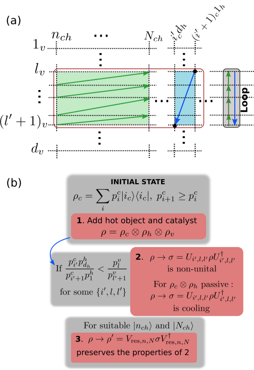
In Fig. 3(a) we apply the $\textrm{ln}(p^{ch})\times\textrm{ln}(p^{v})$ diagram to illustrate the currents generated by a catalytic unitary $U_{i^{\prime},l,l^{\prime}}\oplus V_{\textrm{res},n,N}$. Since each $V_{|n_{ch}(k+1)_{v}\rangle\leftrightarrow|N_{ch}k_{v}\rangle}$ produces a positive current $J_{|(k+1)_{v}\rangle\rightarrow|k_{v}\rangle}$ iff $p_{n}^{ch}p_{k+1}^{v}>p_{N}^{ch}p_{k}^{v}$, as per Eqs. (15) and (19), it follows that:

$$\textrm{ln}\left(\frac{p_{n}^{ch}}{p_{N}^{ch}}\right)>\textrm{ln}\left(\frac{p_{k}^{v}}{p_{k+1}^{v}}\right).$$ (29)

This inequality implies that the distance between the columns $|n_{ch}\rangle$ and $|N_{ch}\rangle$ is larger than the distance between the rows $|k_{v}\rangle$ and $|(k+1)_{v}\rangle$. Therefore, for $l\leq k\leq l^{\prime}$ all the global currents $J_{|n_{ch}(k+1)_{v}\rangle\rightarrow|N_{ch}k_{v}\rangle}$ are enclosed by horizontal rectangles (with height larger than its width), as shown in Fig. 3(a). Moreover, the associated local currents $J_{|(k+1)_{v}\rangle\rightarrow|k_{v}\rangle}$ are upward-oriented, thus generating the loop with the current $J_{|l_{v}\rangle\rightarrow|(l^{\prime}+1)_{v}\rangle}$.

Before moving to the next section, let us make some important comments:

• The depictions in the $\textrm{ln}(p^{ch})\times\textrm{ln}(p^{v})$ diagram are not intended to be quantitatively precise, but to provide sufficient information at the qualitative level. This means that separations between rows and columns can be imprecise as long as the figure informs correctly which distances are larger and which are smaller.

• Equation (29) is equivalent to the positivity of $J_{|(k+1)_{v}\rangle\rightarrow|k_{v}\rangle}$, given the monotonic character of the natural logarithm. It also implies that if the ratio $\frac{p_{k}^{v}}{p_{k+1}^{v}}$ is too large, for some $k\in\{l,l+1,...,l^{\prime}\}$, it may impossible to satisfy (29) for any $n,N\in\{1,2,...,d_{c}d_{h}\}$. In particular, this is always true if $p_{k}^{v}=1$ and $p_{k+1}^{v}=0$, which describes a pure state $\rho_{v}=|k_{v}\rangle\langle k_{v}|$. We can thus conclude that a catalytic transformation $\rho\rightarrow U\rho U^{\dagger}$, where $U$ satisfies Eq. (22), is possible only if $\rho_{v}$ is a mixed state.

• Figure 3(b) summarizes the essential features of the catalytic transformations addressed in this article. Importantly, Corollaries 1 and 2 provide conditions for $V_{\textrm{res},n,N}$ to preserve the cooling or non-unital character of the initial transformation $\rho\rightarrow U_{i^{\prime},l,l^{\prime}}\rho U_{i^{\prime},l,l^{\prime}}^{\dagger}$. We also stress that while $V_{\textrm{res},n,N}$ possess the specific form (23), its existence is also necessary for the existence of other restoring unitaries characterized in Theorem 1.

5 Catalyst dimension as a resource for cooling and non-unital transformations

Theorem 1 and the derived corollaries (1 and 2) provide sufficient conditions for catalytic transformations, given a fixed state $\rho=\rho_{c}\otimes\rho_{h}\otimes\rho_{v}$. Now, we ask ourselves the following question: given a fixed state $\rho_{c}\otimes\rho_{h}$, is there a catalyst state $\rho_{v}$ such that $\rho\overset{\textrm{CC}}{\longrightarrow}U\rho U^{\dagger}$ or $\rho\overset{\textrm{CNU}}{\longrightarrow}U\rho U^{\dagger}$ are possible? This question is intimately related to the dimension of the catalyst, as seen in the following theorem. The proof can be consulted in Appendix G.

Theorem 2 (catalyst size and catalytic transformations). Given a catalyst dimension $d_{v}=d_{v}^{\ast}$ (where $d_{v}^{\ast}$ is a sufficiently large and explicit dimension derived in Appendix G) and a suitable catalyst state $\rho_{v}=\sum_{k=1}^{d_{v}^{\ast}}p_{k}^{v}|k_{v}\rangle\langle k_{v}|$, the following transformations are possible:

1. Catalytic and cooling transformations: If $\rho_{c}\otimes\rho_{h}$ is a passive state, where $\rho_{h}$ is not fully mixed (i.e. ${\normalcolor p_{1}^{h}>p_{d_{h}}^{h}}$), there exists a explicit state $\rho_{v}$ such that for $\rho=\rho_{c}\otimes\rho_{h}\otimes\rho_{v}$ a transformation $\rho\overset{\textrm{CC}}{\longrightarrow}U\rho U^{\dagger}$ can be implemented.

2. Catalytic and non-unital transformations: If $\rho_{c}$ satisfies $p_{1}^{c}>p_{i^{\prime}}^{c}$ or $p_{i^{\prime}+1}^{c}>p_{d_{c}}^{c}$ for some $i^{\prime}\in\{1,2,...,d_{c}-1\}$, and $d_{c}\geq 3$, there exists a explicit state $\rho_{v}$ such that for $\rho=\rho_{c}\otimes\rho_{v}$ a transformation $\rho\overset{\textrm{CNU}}{\longrightarrow}U\rho U^{\dagger}$ can be implemented.

According to Theorem 2, a sufficiently large catalyst allows catalytic transformations for almost any initial state $\rho_{c}\otimes\rho_{h}$. In particular, Statement 1 implies that any hot object with non-degenerate energy spectrum and finite temperature suffices to perform catalytic cooling. Furthermore, Statement 2 tells us that, in the case of non-unital transformations, the hot object can be ignored if $\rho_{c}$ satisfies the mentioned properties. In other words, there exists a unitary $U$ that performs the transformation and acts on $\mathcal{H}_{c}\otimes\mathcal{H}_{v}$ , as shown in Appendix G2.

It is also worth pointing out that a harmonic oscillator constitutes an example of universal catalyst, in the sense that it can be prepared in any required state $\rho_{v}$. To that end, we only need to populate $d_{v}^{\ast}$ of its levels with the eigenvalues of $\rho_{v}$, irrespective of how large is $d_{v}^{\ast}$.

6 Examples of catalytic cooling

In the first two parts of this section we illustrate different catalytic and cooling transformations that stem from Theorem 2, some of which rely on restoring unitaries that generalize those based on Eq. (23). The last section (VI-C) explores the new scenario of cooling enhancement via a catalyst, not considered until now. Before proceeding with the examples, we shall briefly explain how the aforementioned generalization takes place.

The essential idea is that, depending on the eigenvalues of $\rho$, there could be various restoring unitaries of the form (23). This would occur if for several pairs of states $(|n_{ch}\rangle,|N_{ch}\rangle)$ all the partial swaps in the set $\{V_{|n_{ch}(k+1)_{v}\rangle\leftrightarrow|N_{ch}k_{v}\rangle}\}_{k=l}^{l^{\prime}}$ can generate positive currents $J_{|(k+1)_{v}\rangle\rightarrow|k_{v}\rangle}$. Under this condition, we show in Appendix H that another restoring unitary can be obtained as

$$V_{\textrm{res}} =\oplus_{n,N}V_{\textrm{res,}n,N}$$

$$=\oplus_{k=l}^{l^{\prime}}\left(\oplus_{n,N}V_{|n_{ch}(k+1)_{v}\rangle\leftrightarrow|N_{ch}k_{v}\rangle}\right).$$ (30)

In Eq. (30), as well as in Eq. (23), the swap intensities are implicit and can take any value $0<r\leq 1$. However, as long as $p_{n}^{ch}p_{k+1}^{v}-p_{N}^{ch}p_{k}^{v}>0$ for any pair $(|n_{ch}\rangle,|N_{ch}\rangle)$ in the sum, it is always possible to tune these intensities in such a ways that $U=U_{i^{\prime},l,l^{\prime}}\oplus V_{\textrm{res}}$ gives rise to a catalytic transformation (cf. Appendix H).

To illustrate the usefulness of Eq. (30) we now generalize the controlled unitaries (26) (assuming that they are valid restoring unitaries, as per Corollary 1) to a restoring unitary $V_{\textrm{res}}$ that acts on $\mathcal{H}_{h}\otimes\mathcal{H}_{v}$. Such a property is important because it means that in this case the cold object is not involved in the restoration of the catalyst, and therefore a two-body interaction with the hot object is sufficient. Since the set $\{V_{\textrm{res},|i_{c}^{\prime\prime}\rangle}\}_{i^{\prime\prime}=1}^{d_{c}}$ constitutes a family of restoring unitaries, $\oplus_{i^{\prime\prime}}V_{\textrm{res},|i_{c}^{\prime\prime}\rangle}$ is also a restoring unitary of the form (30), where $|n_{ch}\rangle$ and $|N_{ch}\rangle$ are related to $i^{\prime\prime}$ through (24). In addition, from (26) it readily follows that

$$\oplus_{i^{\prime\prime}}V_{\textrm{res},|i_{c}^{\prime\prime}\rangle} =\mathbb{I}_{c}\otimes\left(\oplus_{k=l}^{l^{\prime}}V_{|1_{h}(k+1)_{v}\rangle\leftrightarrow|d_{h}k_{v}\rangle}\right)$$

$$=V_{\textrm{res},hv},$$ (31)

where the subindex $hv$ indicates that $V_{\textrm{res},hv}$ acts on $\mathcal{H}_{h}\otimes\mathcal{H}_{v}$.

6.1 Optimal catalytic cooling of a qubit using another qubit as hot object

Based on Statement 1 of Theorem 2, our goal now is to explore how catalysts of different dimensions perform to cool a qubit using as hot object another qubit, with respective initial states $\rho_{c}=\sum_{i=1}^{2}p_{i}^{c}|i_{c}\rangle\langle i_{c}|$ and $\rho_{h}=\sum_{j=1}^{2}p_{i}^{h}|j_{h}\rangle\langle j_{h}|$. In this case, the passivity constraint for $\rho_{c}\otimes\rho_{h}$ yields the simple inequality $p_{2}^{c}\leq p_{2}^{h}$. Moreover, the cooling effect is due to the unitary $U_{i^{\prime},1,d_{v}-1}$ (cf. Eq. (20)), which only admits the value $i^{\prime}=1$ for dimension $d_{c}=2$. Assuming $\varepsilon_{1}^{c}=0$, Eq. (21) yields

$$\Delta\bigl{\langle}H_{c}\bigr{\rangle} =\textrm{Tr}\left[H_{c}\left(U\rho U^{\dagger}-\rho\right)\right]$$

$$=-J_{\textrm{cool}}\varepsilon_{2}^{c},$$

where $U=U_{1,1,d_{v}-1}\oplus V_{\textrm{res},hv}$ and $J_{\textrm{cool}}=J_{|2_{c}\rangle\rightarrow|1_{c}\rangle}$ is the cooling current induced by $U_{1,1,d_{v}-1}$.

While in Theorem 2 we refer to a certain catalyst state that lifts the passivity constraint by enabling cooling (Statement 1), here we are interested in an optimal state. The associated optimization means that, if cooling is possible for a certain dimension $d_{v}^{\ast}$, we maximize it over the eigenvalues $\{p_{k}^{v}\}_{k}$ of full-rank states $\rho_{v}=\sum_{k=1}^{d_{v}^{\ast}}p_{k}^{v}|k_{v}\rangle\langle k_{v}|$, which amounts to maximize $J_{\textrm{cool}}$ over $\{p_{k}^{v}\}_{k}$. Full-rank states are chosen because the explicit state $\rho_{v}$ that allows us to prove Theorem 2 is of this form.

Figure 4: Optimal catalytic cooling of a qubit using another qubit as hot object. (a), (b) and (c) show the cooling currents obtained with catalyst states $\rho_{v}$ of dimensions $2\leq d_{v}^{\ast}\leq 10$, and hot qubits with initial (excited) populations $p_{2}^{h}=0.4$, $p_{2}^{h}=0.3$, and $p_{2}^{h}=0.1$, respectively. The inset in (a) shows the cooling regions corresponding to $2\leq d_{v}^{\ast}\leq 5$, where $d_{v}^{\ast}$ is sufficiently large to allow cooling. Since the maxima of $J_{\textrm{cool}}^{\textrm{max}}$ in (a), (b) and (c) are achieved for $p_{2}^{c}=p_{2}^{h}$ and $d_{v}^{\ast}=2,3$, in (d) we consider the cooling using a two-level catalyst ($d_{v}^{\ast}=2$) and a hot qubit such that $p_{2}^{c}=p_{2}^{h}$. The black dashed line depicts the initial ground population of the cold qubit and the blue curve is the corresponding final population.

In Appendix I we obtain the maximum current $J_{\textrm{cool}}$:

$$J_{\textrm{cool}}^{\textrm{max}}=\left[\frac{(\zeta-1)p_{2}^{h}\left(p_{2}^{c}\zeta^{d_{v}^{\ast}}-p_{1}^{c}\right)}{\zeta^{d_{v}^{\ast}-1}(\zeta-1)+p_{1}^{c}(\zeta^{d_{v}^{\ast}-1}-1)}\right]\bar{p}_{1}^{v},$$ (32)

where $\zeta\equiv\frac{p_{1}^{h}}{p_{2}^{h}}$ and the superscripts in $\zeta$ indicate powers.The optimal eigenvalues are denoted as $\{\bar{p}_{k}^{(v)}\}_{k}$ and are also derived in the same appendix. For these eigenvalues, the unitary that generates the current (32) is given by

$$U =\mathcal{U}_{1,1,d_{v}^{\ast}-1}\oplus V_{\textrm{res},hv},$$ (33)

$$V_{\textrm{res},hv} =\oplus_{k=1}^{d_{v}^{\ast}-1}\mathcal{V}_{|1_{h}(k+1)_{v}\rangle\leftrightarrow|2_{h}k_{v}\rangle}.$$ (34)

This implies that optimal cooling is achieved by setting $r=1$ for all the two-level unitaries that compose $U$. This results in a direct sum of swaps, and consequently $U$ in Eq. (33) is a permutation of the eigenstates of $\rho$.

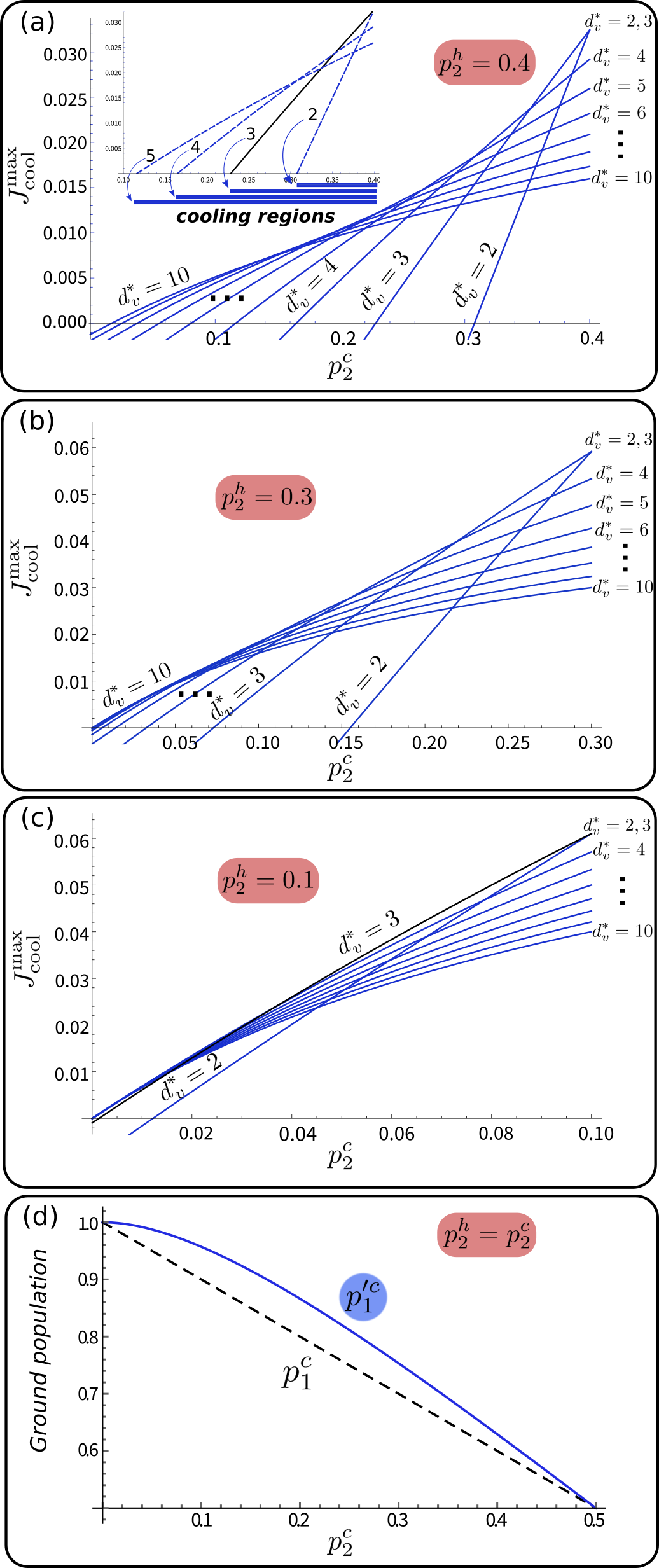
Figure 4 shows plots of $J_{\textrm{cool}}^{\textrm{max}}$ and the final ground population $p_{1}^{\prime c}$, for different values of $p_{2}^{h}$ and catalyst of dimensions $2\leq d_{v}^{\ast}\leq 10$. Each solid curve in Figs. 4(a)-(c) depicts the maximum cooling current corresponding to a different value of $d_{v}^{\ast}$. Moreover, $J_{\textrm{cool}}^{\textrm{max}}$ in Eq. (32) is plotted as a function of $0\leq p_{2}^{c}\leq p_{2}^{h}$, which constitutes the interval where $\rho_{c}\otimes\rho_{h}$ is passive. In Fig. 4(a) we can see that as $d_{v}^{\ast}$ increases the interval of $p_{2}^{c}$ where $J_{\textrm{cool}}^{\textrm{max}}$ is positive also increases. Since $J_{\textrm{cool}}^{\textrm{max}}<0$ means that population would be transferred from the ground state to the excited state of the cold qubit, thereby heating it up, the “cooling region” is described by the condition $J_{\textrm{cool}}^{\textrm{max}}\geq 0$. The inset in Fig. 4(a) shows more clearly the cooling regions (blue bars) corresponding to states of dimensions $2\leq d_{v}^{\ast}\leq 5$. The enlargement of these regions as $d_{v}^{\ast}$ increases indicates that larger catalysts may allow cooling in regimes not accessible to small catalysts, characterized by $p_{2}^{c}\ll p_{2}^{h}$. On the other hand, for $p_{2}^{c}=p_{2}^{h}$ it is remarkable that $J_{\textrm{cool}}^{\textrm{max}}$ is maximized by $d_{v}^{\ast}=2$ and $d_{v}^{\ast}=3$, and decreases for larger values of $d_{v}^{\ast}$. This implies that in such a case the smallest possible catalyst, corresponding to a two-level system, is sufficient to achieve maximum cooling. Moreover, it is also worth noting that the cooling current corresponding to $d_{v}^{\ast}=3$ always surpasses the current corresponding to $d_{v}^{\ast}=2$ (except for $p_{2}^{c}=p_{2}^{h}$).

Figures 4(b) and 4(c) display the same pattern that characterizes Fig. 4(a). In particular, notice that in both cases a catalyst of dimension $d_{v}^{\ast}=10$ allows to cool for almost any value of $p_{2}^{c}$. In Fig. 4(c) we also see that a catalyst with $d_{v}^{\ast}=3$ (black curve) is essentially as effective as any catalyst of dimension $4\leq d_{v}^{\ast}\leq 10$. Accordingly, in this case a three-level catalyst is optimal for almost any value of $p_{2}^{c}$. Figure 4(d) shows the initial and final ground populations as a function of $p_{2}^{c}$, if the populations of the hot and cold qubits always coincide. The final population is computed as $p_{1}^{\prime c}=p_{1}^{c}+J_{\textrm{cool}}^{\textrm{max}}$, where $J_{\textrm{cool}}^{\textrm{max}}$ is the cooling current attained for $d_{v}^{\ast}=2$ (or $d_{v}^{\ast}=3$).

6.2 Catalytic increment of the ground population of the cold object

Reducing the average energy of the cold object is not the only approach for cooling. Alternatively, increasing the ground population of a quantum system has also been considered as a way to cool it [43]. As the following proposition shows, such an increment constitutes yet another example of useful non-unital transformation.

Proposition 1. Any transformation $\rho_{c}\rightarrow\rho^{\prime}_{c}$ such that $\textrm{Tr}\left(|1_{c}\rangle\langle 1_{c}|\rho^{\prime}_{c}\right)>\textrm{Tr}\left(|1_{c}\rangle\langle 1_{c}|\rho_{c}\right)$ is a non-unital transformation.

Proof. To prove this proposition we use the fact that the aforementioned transformation can always be cast as a cooling transformation, given a suitable energy spectrum $\{\varepsilon_{i}^{c}\}_{i}$. Specifically, we can consider a Hamiltonian $H_{c}=\sum_{i=1}^{d_{c}}\varepsilon_{i}^{c}|i_{c}\rangle\langle i_{c}|$ with eigenvalues that satisfy $\varepsilon_{1}^{c}<\varepsilon_{2}^{c}$, and $\varepsilon_{2}^{c}=\varepsilon_{i}^{c}$ for $2\leq i\leq d_{c}$. These eigenvalues ensure that the state $\rho_{c}=\sum_{i}p_{i}^{c}|i_{c}\rangle\langle i_{c}|$ (with $p_{i}^{c}\geq p_{i+1}^{c}$) is passive. Denoting the population variation corresponding to $|i_{c}\rangle$ as $\Delta p_{i}^{c}$, and applying probability conservation $\Delta p_{1}^{c}=-\sum_{i=2}^{d_{c}}\Delta p_{i}^{c}$, we have that $\sum_{i=2}^{d_{c}}\Delta p_{i}^{c}\varepsilon_{i}^{c}=-\Delta p_{1}^{c}\varepsilon_{2}^{c}$. Accordingly,

$$\Delta\bigl{\langle}H_{c}\bigr{\rangle} =\Delta p_{1}^{c}\varepsilon_{1}^{c}+\sum_{i=2}^{d_{c}}\Delta p_{i}^{c}\varepsilon_{i}^{c}$$

$$=\Delta p_{1}^{c}(\varepsilon_{1}^{c}-\varepsilon_{2}^{c}),$$ (35)

which is negative for any increment $\Delta p_{1}^{c}=\textrm{Tr}\left(|1_{c}\rangle\langle 1_{c}|(\rho^{\prime}_{c}-\rho_{c})\right)>0$. Since any cooling transformation is non-unital (cf. Definition 3 and subsequent comments), any transformation that increases the ground population is non-unital.

In Appendix G2 (Corollary 3) we show how the existence of a catalytic transformation that satisfies $\Delta p_{1}^{c}>0$ follows from the constructive proof for Statement 2 of Theorem 2. Accordingly, a catalytic increment of $\bigl{\langle}|1_{c}\rangle\langle 1_{c}|\bigr{\rangle}$ can be performed via a transformation $\rho_{c}\otimes\rho_{v}\rightarrow U\rho_{c}\otimes\rho_{v}U^{\dagger}$, using a sufficiently large catalyst, and without requiring the hot object. Corollary 3 indicates that for this to be possible it suffices to consider a cold object whose eigenvalues satisfy $p_{2}^{c}>p_{d_{c}}^{c}$.

6.3 Catalyst-aided enhancement of cooling

The usefulness of catalysts is not restricted to the implementation of transformations that are forbidden without the utilization of these systems. Here we show that cooling can be catalytically enhanced, even if the hot object is sufficient to achieve a certain level of cooling. This is formally stated in the following theorem, whose proof consists of two parts and is given in Appendix J. First, we derive a global unitary that provides optimal cooling without using the catalyst, and then construct a catalytic transformation that yields the enhancement. We also remark that optimal cooling unitaries for a qubit interacting with a finite environment have been shown in Ref. [53]. However, we present a derivation based on passivity, in order to maintain a self-contained structure.

Theorem 3 (cooling enhancement with a catalyst). Let $\rho_{c}$ be a passive state of a qubit, and let $\rho_{c}\otimes\rho_{h}$ be a non-passive state, where $\rho_{h}=\sum_{j=1}^{d_{h}}p_{j}^{h}|j_{h}\rangle\langle j_{h}|$ is the state of a hot object of even dimension $d_{h}\geq 4$. If $d_{v}$ is sufficiently large and $p_{1}^{h}>p_{d_{h}/2}^{h}$ or $p_{d_{h}/2}^{h}>p_{d_{h}}^{h}$, there exist a explicit catalyst state that increases the optimal cooling achieved with the hot object alone. That is, there exists a catalytic transformation $\rho=\rho_{c}\otimes\rho_{h}\otimes\rho_{v}\overset{\textrm{CC}}{\longrightarrow}\rho^{\prime}=U\rho U^{\dagger}$, where $\rho_{v}=\sum_{k=1}^{d_{v}}|k_{v}\rangle\langle k_{v}|$ and $\textrm{Tr}\left(H_{c}\rho^{\prime}\right)<\textrm{min}_{U_{ch}}\textrm{Tr}\left(H_{c}U_{ch}\rho_{c}\otimes\rho_{h}U_{ch}^{\dagger}\right)$, for arbitrary unitaries $U_{ch}$ acting on $\mathcal{H}_{c}\otimes\mathcal{H}_{h}$.

Figure 5: Catalytic enhancement of cooling using a qubit as catalyst and a three-level system as hot object. (a) Initial ground population of the cold qubit (cyan dashed), ground population after optimal cooling without the catalyst (blue dashed-dotted), and ground population after a subsequent catalytic and cooling transformation (black solid). The parameter $e^{-\beta_{h}\varepsilon_{2}^{h}}=0.01$ is fixed. (b) Schematic representation of the catalytic transformation. (Left) $\textrm{ln}(p^{ch})\times\textrm{ln}(p^{v})$ diagram for the non-passive state $\rho_{c}\otimes\rho_{h}$ (note that $1_{c}3_{h}$ is at the right of $2_{c}1_{h}$). The distance $\beta_{h}\omega_{1,2}^{h}\equiv\beta_{h}(\varepsilon_{2}^{h}-\varepsilon_{1}^{h})$ tends to zero to comply with the degeneracy $\varepsilon_{2}^{h}=\varepsilon_{1}^{h}$. (Right) After the optimal cooling using $\mathcal{U}_{|2_{c}1_{h}\rangle\leftrightarrow|1_{c}3_{h}\rangle}$ the unitary $U$ in (37) is applied on the resulting state. The resulting currents are depicted in the diagram below.

While Theorem 3 concerns catalytic enhancement of cooling using hot objects of even dimension, we also show that this is possible by means of a three-level hot object. The following example is based on a three-level system with Hamiltonian $H_{h}=\sum_{j=1}^{3}\varepsilon_{j}^{h}|j_{h}\rangle\langle j_{h}|$, with degeneracy $\varepsilon_{1}^{h}=\varepsilon_{2}^{h}=0$ and a non-null energy gap $\omega_{2,3}^{h}=\varepsilon_{3}^{h}-\varepsilon_{2}^{h}>0$. We characterize cooling in terms of the final ground population of the cold qubit, keeping in mind that in this case the minimization of the average energy amounts to maximize the ground population.

In Fig. 5(a) we show the maximum cooling attainable via a hot object prepared in the thermal state $\rho_{h}=\frac{e^{-\beta_{h}H_{h}}}{\textrm{Tr}(e^{-\beta_{h}H_{h}})}$, as well as an additional cooling through a transformation that employs a qubit as catalyst. The total transformation is thus a composition $\rho\rightarrow\sigma_{ch}\otimes\rho_{v}\rightarrow\rho^{\prime}$, where $\rho=\rho_{c}\otimes\rho_{h}\otimes\rho_{v}$, $\sigma_{ch}=U_{ch}\rho_{c}\otimes\rho_{h}U_{ch}^{\dagger}$, being $U_{ch}$ a unitary that optimally cools $\rho_{c}$ using $\rho_{h}$, and $\rho^{\prime}=U\sigma_{ch}\otimes\rho_{v}U^{\dagger}$, being $U$ a catalytic and cooling unitary. Following Eq. (3), $\rho_{c}\otimes\rho_{h}$ is non-passive with respect to $H_{c}$ iff $\frac{p_{1}^{c}}{p_{2}^{c}}<\frac{p_{1}^{h}}{p_{3}^{h}}$, which implies also that the swap $\mathcal{U}_{|2_{c}1_{h}\rangle\leftrightarrow|1_{c}3_{h}\rangle}$ cools down the cold qubit by the amount $\Delta\bigl{\langle}H_{c}\bigr{\rangle}=(p_{2}^{c}p_{1}^{h}-p_{1}^{c}p_{3}^{h})(\varepsilon_{1}^{c}-\varepsilon_{2}^{c})$. In fact, it is not difficult to corroborate that this swap corresponds to the optimal cooling unitary $U_{ch}^{\textrm{opt}}$. To that end we show that the application of $\mathcal{U}_{|2_{c}1_{h}\rangle\leftrightarrow|1_{c}3_{h}\rangle}$ yields a passive state with respect to $H_{c}$. Since the only effect of $\mathcal{U}_{|2_{c}1_{h}\rangle\leftrightarrow|1_{c}3_{h}\rangle}$ is to exchange the eigenvalues of $|2_{c}1_{h}\rangle$ and $|1_{c}3_{h}\rangle$, the resulting state $\sigma_{ch}$ reads

$$\sigma_{ch} =|1_{c}\rangle\langle 1_{c}|\otimes\left(\sum_{j=1}^{2}p_{1}^{c}p_{j}^{h}|j_{h}\rangle\langle j_{h}|+p_{2}^{c}p_{1}^{h}|3_{h}\rangle\langle 3_{h}|\right)$$

$$\quad+|2_{c}\rangle\langle 2_{c}|\otimes\left(p_{1}^{c}p_{3}^{h}|1_{h}\rangle\langle 1_{h}|+\sum_{j=2}^{3}p_{2}^{c}p_{j}^{h}|j_{h}\rangle\langle j_{h}|\right).$$ (36)

This state is such that all the eigenvalues in the first line of Eq. (36) are larger or equal than the eigenvalues in the second line: Clearly, $p_{1}^{c}p_{2}^{h}\geq p_{1}^{c}p_{3}^{h}$ and $p_{1}^{c}p_{2}^{h}\geq p_{2}^{c}p_{2}^{h}$, which guarantees that the aforementioned property holds when comparing the eigenvalues in the sum $\sum_{j=1}^{2}p_{1}^{c}p_{j}^{h}|j_{h}\rangle\langle j_{h}|$ with all the eigenvalues of the second line. Furthermore, $p_{2}^{c}p_{1}^{h}\geq p_{2}^{c}p_{2}^{h}$, which guarantees that $p_{2}^{c}p_{1}^{h}$ is larger or equal than the eigenvalues in $\sum_{j=2}^{3}p_{2}^{c}p_{j}^{h}|j_{h}\rangle\langle j_{h}|$, and $p_{2}^{c}p_{1}^{h}>p_{1}^{c}p_{3}^{h}$ is equivalent to the non-passivity of $\rho_{c}\otimes\rho_{h}$. In this way, the passivity of $\sigma_{ch}$ can be concluded by noting that $[H_{c}\otimes\mathbb{I}_{h},\sigma_{ch}]=0$ and that the eigenvalues of $H_{c}\otimes\mathbb{I}_{h}$ regarding eigenstates in the first (second) line of (36) are all equal to $\varepsilon_{1}^{c}$ ($\varepsilon_{2}^{c}$). Hence, the eigenvalues of $\sigma_{ch}$ are non-increasing with respect to those of $H_{c}\otimes\mathbb{I}_{h}$.

In Fig. 5(a) we set $e^{-\beta_{h}\varepsilon_{3}^{h}}=0.01$, thereby fixing the eigenvalues of $\rho_{h}$ (taking into account the degeneracy $\varepsilon_{1}^{h}=\varepsilon_{2}^{h}$). The blue dash-dotted curve depicts the ground population after the initial transformation $\rho\rightarrow\sigma_{ch}\otimes\rho_{v}$, and the black solid curve stands for the final population achieved with the subsequent transformation $\sigma_{ch}\otimes\rho_{v}\rightarrow\rho^{\prime}$. This transformation is executed through a permutation

$$U =\mathcal{U}_{|2_{c}2_{h}1_{v}\rangle\leftrightarrow|1_{c}3_{h}2_{v}\rangle}\oplus V_{\textrm{res}},$$ (37)

$$V_{\textrm{res}} =\mathcal{V}_{|1_{c}1_{h}2_{v}\rangle\leftrightarrow|1_{c}3_{h}1_{v}\rangle}\oplus\mathcal{V}_{|2_{c}2_{h}2_{v}\rangle\leftrightarrow|2_{c}3_{h}1_{v}\rangle}$$

$$=\left[|1_{c}\rangle\langle 1_{c}|\otimes\mathcal{V}_{|1_{h}2_{v}\rangle\leftrightarrow|3_{h}1_{v}\rangle}+|2_{c}\rangle\langle 2_{c}|\otimes\mathbb{I}_{hv}\right]$$

$$\quad\oplus\left[|2_{c}\rangle\langle 2_{c}|\otimes\mathcal{V}_{|2_{h}2_{v}\rangle\leftrightarrow|3_{h}1_{v}\rangle}+|1_{c}\rangle\langle 1_{c}|\otimes\mathbb{I}_{hv}\right],$$ (38)

which is derived in Appendix J2 . Noting that $[V_{\textrm{res}},H_{c}]=0$, we have that the only contribution to $\Delta_{U}\bigl{\langle}H_{c}\bigr{\rangle}\equiv\textrm{Tr}\left[H_{c}\left(U\sigma_{ch}\otimes\rho_{v}U^{\dagger}-\sigma_{ch}\otimes\rho_{v}\right)\right]$ comes from the swap $\mathcal{U}_{|2_{c}2_{h}1_{v}\rangle\leftrightarrow|1_{c}3_{h}2_{v}\rangle}$. Since $\mathcal{U}_{|2_{c}2_{h}1_{v}\rangle\leftrightarrow|1_{c}3_{h}2_{v}\rangle}$ reduces $\bigl{\langle}H_{c}\bigr{\rangle}$, as shown in J2, it follows that $\Delta_{U}\bigl{\langle}H_{c}\bigr{\rangle}<0$. Specifically, this variation is given by

$$\Delta_{U}\bigl{\langle}H_{c}\bigr{\rangle}=\left(\frac{p_{2}^{h}p_{1}^{c}-p_{3}^{h}p_{2}^{c}}{(1+p_{2}^{c})p_{2}^{h}+p_{2}^{c}}\right)p_{2}^{c}p_{2}^{h}(\varepsilon_{1}^{c}-\varepsilon_{2}^{c}).$$ (39)

Figure 6: Initially extracted heat (dashed blue curves) and total extracted heat (solid black curves), including the contribution from the catalytic transformation. The parameter $e^{-\beta_{c}\varepsilon_{2}^{c}}$ has the fixed values 0.1 (a), 0.4 (b), and 0.8 (c).

Remarkably, we see from Fig. 5(a) that for low temperatures ($\beta_{c}$ large) the increment of $p_{1}^{c}$ due to the catalytic transformation is comparable to that achieved via optimal cooling without the catalyst. Moreover, the cooling enhancement provided by the catalyst is significant in all the temperature range.

Figure 5(b) illustrates the global currents generated by all the swaps in $U$, using a $\textrm{ln}(p^{ch})\times\textrm{ln}(p^{v})$ diagram of the state $\sigma_{ch}\otimes\rho_{v}$ (diagram at the right hand side). The columns in this diagram are ordered taking into account the sorting corresponding to the initial state $\rho_{c}\otimes\rho_{h}$ (top arrangement). In this way, the sorting associated with $\sigma_{ch}$ is obtained by simply exchanging the columns $2_{c}1_{h}$ and $1_{c}3_{h}$, which describes the effect of the swap $U_{ch}=\mathcal{U}_{|2_{c}1_{h}\rangle\leftrightarrow|1_{c}3_{h}\rangle}$. The swap $\mathcal{U}_{|2_{c}2_{h}1_{v}\rangle\leftrightarrow|1_{c}3_{h}2_{v}\rangle}$ generates the cooling current (blue arrow), and $\mathcal{V}_{|1_{c}1_{h}2_{v}\rangle\leftrightarrow|1_{c}3_{h}1_{v}\rangle}$ ($\mathcal{V}_{|2_{c}2_{h}2_{v}\rangle\leftrightarrow|2_{c}3_{h}1_{v}\rangle}$) generates the current depicted by the left (right) green arrow.

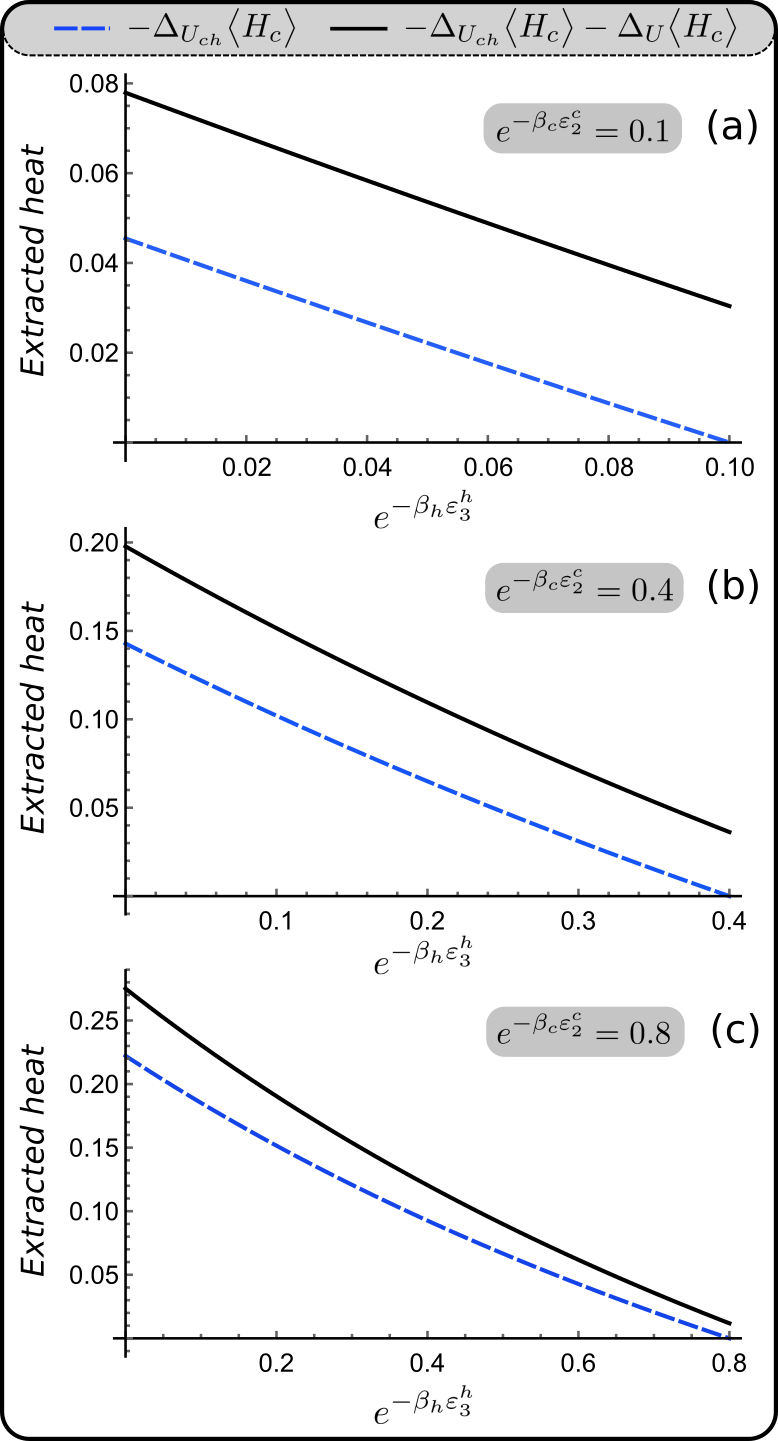
In Fig. 6 we plot the initially extracted heat $-\Delta_{U_{ch}}\bigl{\langle}H_{c}\bigr{\rangle}\equiv\textrm{Tr}[H_{c}(\rho_{c}\otimes\rho_{h}-U_{ch}\rho_{c}\otimes\rho_{h}U_{ch}^{\dagger})]$, and the total extracted heat $-\Delta_{U_{ch}}\bigl{\langle}H_{c}\bigr{\rangle}-\Delta_{U}\bigl{\langle}H_{c}\bigr{\rangle}$, obtained after the application of $U$. In these plots $e^{-\beta_{c}\varepsilon_{2}^{c}}$ is fixed, and we instead vary the parameter $e^{-\beta_{h}\varepsilon_{3}^{h}}$. The maximum of $e^{-\beta_{h}\varepsilon_{3}^{h}}$ corresponds to $e^{-\beta_{c}\varepsilon_{2}^{c}}$, where $\Delta_{U_{ch}}\bigl{\langle}H_{c}\bigr{\rangle}=0$ and it is impossible to cool without the catalyst (i.e. where $\rho_{c}\otimes\rho_{h}$ becomes passive). Although the catalytic contribution is again more significant at low temperatures, evidently the relative contribution with respect to $-\Delta_{U_{ch}}\bigl{\langle}H_{c}\bigr{\rangle}$ is larger at higher temperatures, where the state $\rho_{c}\otimes\rho_{h}$ approaches the passive configuration.

7 Cooling of many qubits and catalytic advantage

In this section we present another example of catalytic enhancement for cooling. This example is special in the sense that it illustrates how the reusable character of the catalyst can be fully exploited in a scenario that involves the cooling of a large number of qubits. Similarly to the problem considered in Sect. VI-C, the cooling of these systems can be performed without a catalyst. However, under certain circumstances the catalyst allows to extract as much heat as twice what is possible if it is not used. In addition, we will see that such a catalytic advantage takes place through cooling cycles that require at most three-body interactions, while arbitrary many-body interactions are assumed in the cooling scenario that does not involve the catalyst.

7.1 Catalytic cooling vs. cooling using many-body interactions

Consider the scenario schematically depicted in Fig. 7. The goal is to cool as much as possible a group of $N_{c}$ qubits, using a group of $N_{h}$ qubits that play the role of a hot environment. All the qubits start at the same inverse temperature $\beta$ and have identical energy spectrum. Assuming zero ground eigenenergy and energy gap equal to one, the Hamiltonians of the $i$th cold and hot qubits are respectively $H_{c}^{(i)}=|2_{c}\rangle_{i}\langle 2_{c}|$ and $H_{h}^{(i)}=|2_{h}\rangle_{i}\langle 2_{h}|$. The total Hamiltonian for the $X=C,H$ group is $H_{X}=\sum_{i=1}^{N_{x}}|2_{x=c,h}\rangle_{i}\langle 2_{x=c,h}|$, and the global initial state is a product of thermal states $\rho_{CH}=\rho_{C}\otimes\rho_{H}$, where $\rho_{X}=\frac{e^{-\beta H_{X}}}{\textrm{Tr}(e^{-\beta H_{X}})}=\rho_{x}^{\otimes N_{x}}$ and $\rho_{x=c,h}=\sum_{i=1}^{2}p_{i}^{x}|i_{x}\rangle\langle i_{x}|$. Given a fixed number qubits $N=N_{c}+N_{h}$, we now describe the two cooling strategies illustrated in Fig. 7.

1. Many-body cooling (MBC) strategy: subsets of $2\leq k\leq N_{h}$ qubits from the hot group are used to optimally cool individual qubits in the cold group, through optimal unitary transformations. Each qubit is cooled down only one time and the hot qubits pertaining to different subsets are all different (this implies that hot qubits are also used only once). Note also that $k\geq 2$, since all the qubits have identical states and therefore cooling is forbidden for $k=1$ (since $\rho_{c}^{(i)}\otimes\rho_{h}^{(i)}$ is passive).

2. Catalytic cooling (CC) strategy: a catalyst is employed to cool down single qubits from the cold group, using only one hot qubit per cold qubit. As with the MBC strategy, there is no re-usage of hot qubits and each cold qubit is cooled down only one time.

Figure 7: Many-body cooling (a) and catalytic cooling (b) strategies, to cool a group of $N_{c}$ qubits using $N_{h}$ qubits as hot environment. Each sequence of dots represents the total number of qubits $N=N_{c}+N_{h}$. From top to bottom: $N_{c}=8$ (first two sequences), $N_{c}=6$ (third and fourth sequences), and $N_{c}=12$. (a) Different partitions of the environment into cooling subsets. In the top sequence two qubits are cooled using two subsets of $k_{0}=2$ and $k_{1}=14$ hot qubits. The next sequence shows the optimal partition $\boldsymbol{K}=\{2,2,...,2\}$ for $N_{c}=N_{h}/2=8$, if the conjecture (44) is true. The same partition is suboptimal for the third sequence, since two hot qubits are unused. (b) In the CC strategy a catalyst (green triangle) allows to cool each qubit using a single hot qubit at a time. In this case the extracted heat is maximized for $N_{c}=N_{h}$.

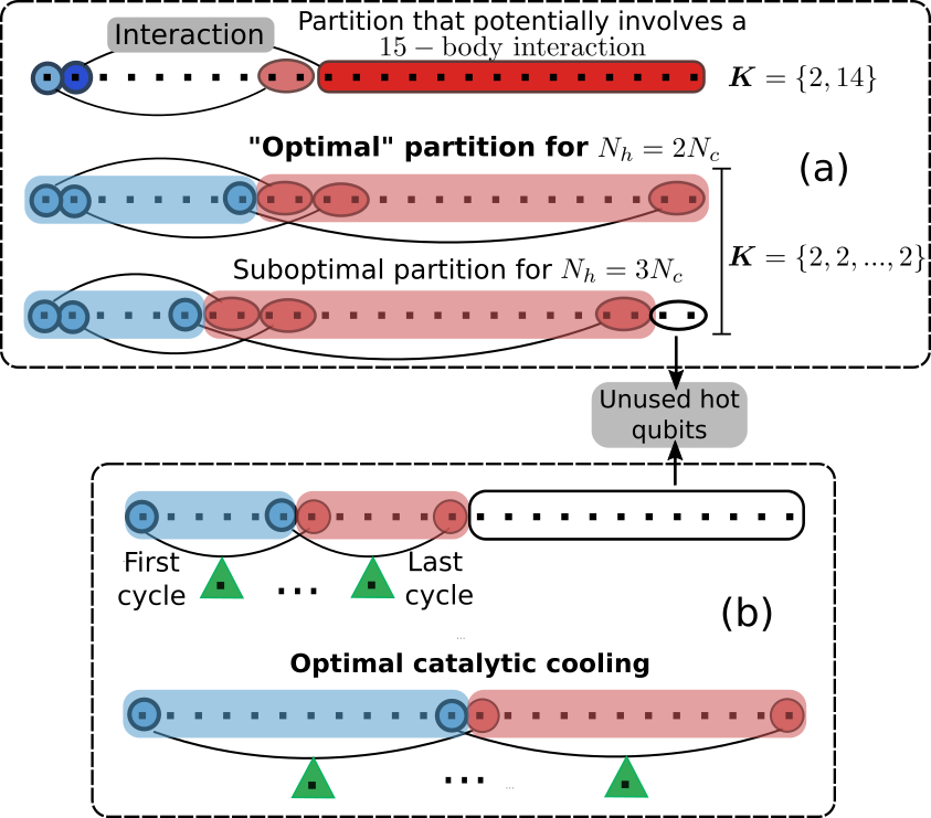
In the MBC strategy the optimal cooling using a subset of $k$ hot qubits involves ($k+1$)-body interactions between these qubits and the corresponding cold qubit. More specifically, such couplings are described by an interaction Hamiltonian that contains products of the form $\otimes_{i=1}^{k+1}B_{i}$, where $B_{i}$ is a non-trivial (i.e. different from the identity) operator on the Hilbert space of the $i$th qubit. On the other hand, the CC strategy is based on the repeated application of the unitary $U$ in Eq. (33), for the case $d_{v}^{\ast}=2$. This means that each cycle implements the optimal cooling of a single qubit using a two-level catalyst and one hot qubit. Importantly, the corresponding restoring unitary involves only a two-body interaction between the catalyst and the hot qubit, while $\mathcal{U}_{1,1,d_{v}^{\ast}-1}$ requires a three-body interaction.

The purpose of any of the described strategies is to reduce as much as possible the total average energy $\bigl{\langle}H_{C}\bigr{\rangle}$ of the cold qubits. Depending on the value of $N_{c}$, the number of qubits that can be cooled may be smaller than $N_{c}$. This limitation is determined by two factors. Namely, the amount of hot qubits available to cool, and the division of these qubits into cooling subsets. For example, if $N_{h}=2$ only one qubit can be cooled using the MBC strategy, while the introduction of the catalyst increases this number to two. That being said, it is important to remark that the following analysis covers all the possible values $1\leq N_{c}\leq N-1$. Therefore, it provides a full picture of the task at hand, including also the situations where all the$N_{c}$ qubits can be cooled. With this observation in mind, the total heat extracted is given by

$$Q_{C}\equiv-\Delta\left\langle H_{C}\right\rangle=\sum_{i=1}^{n_{c}}\Delta p_{1}^{(i)},$$ (40)

where $n_{c}\leq N_{c}$.

7.2 Characterization of MBC

In the case of MBC, the maximum extractable heat $Q_{C}$ can be conveniently addressed by introducing a coefficient that characterizes how efficient is the cooling of a single qubit, with respect to the number of hot qubits employed. This is a natural figure of merit in our scenario, taking into account that the hot qubits constitute a limited resource. Specifically, we define the “$k$-cooling coefficient” $\xi_{\textrm{cool}}^{(k)}$ as

$$\xi_{\textrm{cool}}^{(k)}\equiv\frac{Q_{C}^{(k)}}{k},$$ (41)

where $Q_{C}^{(k)}$ is the heat extracted by using a subset of $k\leq N_{h}$ hot qubits.

In the MBC strategy there are many ways in which the $N_{h}$ hot qubits can be divided into cooling subsets. Two of such possibilities are illustrated by the two upper sequences in Fig. 7(a), assuming $N_{c}=8$ and $N_{h}=16$. For the top sequence, one qubit is cooled down using two hot qubits and the cooling of a second qubit resorts to fourteen hot qubits. Intuitively, the second qubit should end up in a colder state because more qubits are invested in its cooling. This also leads us to wonder if it is more profitable to cool less qubits using larger cooling subsets, or more qubits using smaller cooling subsets. Since we are interested in the total heat $Q_{C}$, and not on maximizing the cooling of single qubits, the answer to this puzzle is convoluted. However, as anticipated by the second sequence in Fig. 7(a), at least for $N_{h}=2N_{c}$ using the smallest cooling subsets seems to be the optimal choice. This depends on the validity of a conjecture that we will shortly present (Eq. (44)).

By resorting to the cooling coefficient (41), we can express the total extracted heat as

$$Q_{C}=\sum_{k\in\boldsymbol{K}}Q_{C}^{(k)}=\sum_{k\in\boldsymbol{K}}\xi_{\textrm{cool}}^{(k)}k,$$ (42)

where $\boldsymbol{K}=\{k_{0},k_{1},...\}$ describes a certain partition of the hot group into cooling subsets. In particular, we note that $\sum_{k\in\boldsymbol{K}}k=N_{h}$, and that it is perfectly legitimate to have subsets of different sizes $k_{i}\neq k_{j}$, see Fig 7(a). Given a fixed partition, we also have the bound

$$Q_{C}\leq\left(\textrm{max}_{k\in\boldsymbol{K}}\xi_{\textrm{cool}}^{(k)}\right)\sum_{k\in\boldsymbol{K}}k=\left(\textrm{max}_{k\in\boldsymbol{K}}\xi_{\textrm{cool}}^{(k)}\right)N_{h}.$$ (43)

While the heat $Q_{C}^{(k)}$ is by construction a non-decreasing function of $k$, Fig. 8 provides numerical evidence that $\xi_{\textrm{cool}}^{(k)}$ is maximum for $k=2$. For very large values of $k$ it is also naturally expected that $\xi_{\textrm{cool}}^{(k)}$ tends to zero, since otherwise $Q_{C}^{(k)}$ would be an unbounded quantity (cf. Eq. (41)). Therefore, we conjecture that

$$\xi_{\textrm{cool}}^{(k)}\leq\xi_{\textrm{cool}}^{(2)}=\left(\frac{1-2p_{2}^{c}}{2}\right)p_{1}^{c}p_{2}^{c},$$ (44)

for all $k\geq 2$ and for any $\beta$, which is satisfied for $2\leq k\leq 14$ in Fig. 8. The explicit expression for $\xi_{\textrm{cool}}^{(2)}$ is derived in Appendix G.

Figure 8: Cooling coefficient (41) curves for the cooling of a cold qubit using $2\leq k\leq 14$ hot qubits. Blue solid (red dashed) curves stand for $k$ even (odd). The highest and lowest curves correspond respectively to $\xi_{\textrm{cool}}^{(2)}$ and $\xi_{\textrm{cool}}^{(14)}$. Since $\xi_{\textrm{cool}}^{(k)}<\xi_{\textrm{cool}}^{(2)}$ for any value of $p_{2}^{c}$, this plot shows that the conjecture (44) is true for $2\leq k\leq 14$.

Assuming the validity of the conjecture (44), the bound (43) is saturated if two conditions are met. Namely, if $N_{h}$ is an even number, such that it can be divided into cooling subsets of two qubits, and if all these cooling subsets can be put to use (second sequence in Fig. 7(a)). In such a case a partition $\boldsymbol{K}=\{2,2,...,2\}$ maximizes the extracted heat. The second condition requires that $N_{h}\leq 2N_{c}$, since otherwise $N-2N_{c}$ hot qubits would be left unused. For example, the two unused qubits in Fig. 7(a) (third sequence) could be combined with another pair of qubits to extract more heat from one of the qubits in the cold group.

The third sequence in Fig. 7(a) also illustrates that for $N_{h}\geq 2N_{c}+1$ the partition $\boldsymbol{K}=\{2,2,...,2\}$ allows to cool all the $N_{c}$ qubits. From Eq. (41), the heat extracted in this way would be $2\xi_{\textrm{cool}}^{(2)}N_{c}$. Since we already mentioned that such a partition is suboptimal, we also have the bound $Q_{C}=\sum_{k\in\boldsymbol{K}}\xi_{\textrm{cool}}^{(k)}k\geq 2\xi_{\textrm{cool}}^{(2)}N_{c}$. Summarizing,

$$\textrm{max}_{\boldsymbol{K}}Q_{C} =\xi_{\textrm{cool}}^{(2)}N_{h},\textrm{ if }N_{h}\leq 2N_{c},$$ (45)

$$2\xi_{\textrm{cool}}^{(2)}N_{c}\leq\textrm{max}_{\boldsymbol{K}}Q_{C} \leq\xi_{\textrm{cool}}^{(2)}N_{h},\textrm{ if }N_{h}\geq 2N_{c}+1.$$ (46)

We emphasize that Eq. (45) and the upper bound in (46) depend on the validity of (44). Hence, our following analysis is subject to this condition.

7.3 Advantage of the CC strategy

7.3.1 Characterization

Let us denote as $Q_{C}^{(\textrm{CC})}$ the total extracted heat in this case, to distinguish it from the heat $Q_{C}$ extracted via the MBC strategy. Thanks to the reusable character of the catalyst, the CC strategy operates through cooling cycles where each cycle involves a different pair of qubits, yet the cooling is mediated by the same catalyst. This procedure is depicted in Fig. 7(b).

We consider a two-level catalyst (green triangle in Fig. 7(b)), which allows us to apply Eq. (32) to obtain a simple expression for the heat extracted per cycle. Since $d_{v}^{\ast}=2$ in this case, after setting $p_{2}^{c}=p_{2}^{h}$ (hot qubits identical to the cold qubit) the cooling current (32) takes the simple form $J_{\textrm{cool}}^{\textrm{max}}=\frac{p_{2}^{c}\left(1-2p_{2}^{c}\right)}{1+p_{2}^{c}}\bar{p}_{1}^{v}$. The catalyst population $\bar{p}_{1}^{v}=1-\bar{p}_{2}^{v}$ can be computed from the formula (150) in Appendix I, which is valid for any $d_{v}^{\ast}\geq 2$. This formula yields $\bar{p}_{1}^{v}=\frac{p_{1}^{c}(1+p_{2}^{c})}{1+2p_{2}^{c}p_{1}^{c}}$. In this way, after $n$ cycles the total extracted heat reads

$$Q_{C}^{(\textrm{CC})}=nJ_{\textrm{cool}}^{\textrm{max}}=n\left(\frac{1-2p_{2}^{c}}{1+2p_{1}^{c}p_{2}^{c}}\right)p_{1}^{c}p_{2}^{c},$$ (47)

being $J_{\textrm{cool}}^{\textrm{max}}$ the heat extracted per cycle.

As with the MBC strategy, we are now going to derive expressions that characterize the extracted heat given different relations between $N_{c}$ and $N_{h}$. If $N_{h}\geq N_{c}$, all the $N_{c}$ cold qubits can be catalytically cooled using $N_{c}$ hot qubits (see Fig. 7(b)). In contrast, for $N_{h}\leq N_{c}-1$ we can only cool $N_{h}$ cold qubits but all the $N_{h}$ hot qubits are consumed. Keeping in mind that both scenarios correspond to $n=N_{c}$ and $n=N_{h}$, respectively, Eq. (47) yields

$$Q_{C}^{(\textrm{CC})}=\begin{cases}\begin{array}[]{c}N_{c}\left(\frac{1-2p_{2}^{c}}{1+2p_{1}^{c}p_{2}^{c}}\right)p_{1}^{c}p_{2}^{c},\textrm{ if }N_{h}\geq N_{c},\\ N_{h}\left(\frac{1-2p_{2}^{c}}{1+2p_{1}^{c}p_{2}^{c}}\right)p_{1}^{c}p_{2}^{c},\textrm{ if }{\color[rgb]{0,1,0}\definecolor[named]{pgfstrokecolor}{rgb}{0,1,0}{\normalcolor N_{h}\leq N_{c}-1}},\end{array}\end{cases}$$ (48)

7.3.2 Comparison between CC and MBC

To perform the comparison between CC and MBC we introduce the relative performance ratio

$$\gamma\equiv\frac{Q_{C}^{(\textrm{CC})}}{\textrm{max}_{\boldsymbol{K}}Q_{C}},$$ (49)

where the numerator and the denominator must be evaluated for the same pair $(N_{c},N_{h})$ and the same population $p_{2}^{c}$ (which fully characterizes the individual state of all the qubits).

• For $N_{h}\geq 2N_{c}+1$, $Q_{C}^{(\textrm{CC})}$ is given by the first line of Eq. (49). Moreover, $\textrm{max}_{\boldsymbol{K}}Q_{C}$ is bounded from below by $2\xi_{\textrm{cool}}^{(2)}N_{c}$, according to Eq. (46). This leads to the upper bound

  $$\gamma\leq\frac{Q_{C}^{(\textrm{CC})}}{2\xi_{\textrm{cool}}^{(2)}N_{c}}=\frac{1}{1+2p_{1}^{c}p_{2}^{c}},\textrm{ if }N_{h}\geq 2N_{c}+1,$$ (50)

  where we have also expressed $\xi_{\textrm{cool}}^{(2)}$ as in (44). Clearly, Eq. (50) implies that $\gamma\leq 1$ and therefore MBC outperforms CC for $N_{h}\geq 2N_{c}+1$.

• For $N_{h}\leq 2N_{c}$,$\textrm{max}_{\boldsymbol{K}}Q_{C}$ is given by Eq. (45). If it also holds that $N_{h}\geq N_{c}$, $Q_{C}^{(\textrm{CC})}$ obeys the first line of Eq. (48). Otherwise, $N_{h}\leq N_{c}-1$ and $Q_{C}^{(\textrm{CC})}$ obeys the second line of this equation. In this way, Eqs. (49) and (44) yield

  $$\gamma =\frac{Q_{C}^{(\textrm{CC})}}{\xi_{\textrm{cool}}^{(2)}N_{h}}=\frac{N_{c}}{N_{h}}\left(\frac{2}{1+2p_{1}^{c}p_{2}^{c}}\right),\textrm{ if }N_{c}\leq N_{h}\leq 2N_{c},$$ (51)

  $$\gamma =\frac{Q_{C}^{(\textrm{CC})}}{\xi_{\textrm{cool}}^{(2)}N_{h}}=\frac{2}{1+2p_{1}^{c}p_{2}^{c}}$$

  $$\quad\geq\frac{4}{3},\textrm{ if }N_{h}\leq N_{c}-1.$$ (52)

  where the lower bound in the second line of (52) is obtained from the maximum $\textrm{max}_{\beta}p_{1}^{c}p_{2}^{c}$. Accordingly, for $N_{h}\leq N_{c}-1$ we have that $\gamma>1$ and thus the CC strategy outperforms the MBC strategy.

Let us now address how the relative performance ratio behaves in the remaining interval $N_{c}\leq N_{h}\leq 2N_{c}$. Following Eq. (51), in this case $\gamma>1$ if and only if

$$N_{h}<\frac{2N_{c}}{1+2p_{1}^{c}p_{2}^{c}}.$$ (53)

In the limit $p_{2}^{c}\rightarrow 0$, corresponding to $\beta\rightarrow\infty$, this inequality is equivalent to $N_{h}<2N_{c}$. In the opposite limit $p_{2}^{c}\rightarrow 1/2$, corresponding to $\beta\rightarrow 0$, the previous inequality reads $N_{h}<4N_{c}/3$. Hence, we can conclude that for extremely low temperatures the CC strategy outperforms the MBC strategy in a wider regime. This regime is characterized by the total interval $N_{h}\in[1,N_{c}-1]\cup[N_{c},2N_{c}-1]$, where the first interval is associated with Eq. (52) and the second one is associated with (51). On the other hand, the interval $N_{h}\in[1,N_{c}-1]\cup[N_{c},4N_{c}/3-1]$ characterizes the catalytic advantage in the limit of very large temperatures.

Figure 9: Performance ratio $\gamma$ (49) as a function of $N_{c}/N_{h}$. The top and bottom boundaries of the darker region correspond respectively to the limits $\beta\rightarrow\infty$ and $\beta\rightarrow 0$. The curve inside this region is representative of a fixed $\beta\in(0,\infty)$ and is characterized as follows: the continuous segments ($N_{c}/N_{h}\geq 1/2$) give the exact value of $\gamma$, and the dashed segment ($N_{c}/N_{h}<1/2$) constitutes an upper bound. The CC strategy outperforms the MBC strategy where $\gamma>1$ (light blue area). In particular, $\gamma>1$ for $N_{c}/N_{h}>3/4$, irrespective of the value of $\beta$. For any $N_{c}/N_{h}>1$, $4/3\leq\gamma\leq 2$.

Figure 9 depicts the ratio $\gamma$ and the associated bounds given by Eqs. (50)-(52). The intervals in these equations are re-expressed in terms of $N_{c}/N_{h}$, which is utilized as plotting variable. The light blue area shows the regime where the catalyst provides an advantage with respect to the MBC strategy. The interval $N_{c}/N_{h}\geq 1$ corresponds to Eq. (52), where the advantage is maximum. The ratio in (52) is monotonically increasing with respect to $\beta$, reaching its maximum $\gamma=2$ for $\beta\rightarrow\infty$ ($p_{2}^{c}=0$). For $1/2\leq N_{c}/N_{h}\leq 1$, $\gamma$ increases linearly with $N_{c}/N_{h}$ (cf. (51)), with a slope that varies between 4/3 for $p_{2}^{c}=1/2$ and 2 for $p_{2}^{c}=0$. In particular, this implies that in the interval $N_{c}/N_{h}\in(1/2,3/4)$ the catalytic advantage takes place only if $\beta$ is sufficiently large. For $N_{c}/N_{h}\leq 1/2$, the upper bound (50) varies between 2/3 and 1, corresponding to the high-temperature and low-temperature limits, respectively.

7.3.3 Maximum heat $Q_{C}^{(\textrm{CC})}$ and additional catalytic advantage

We note that, in contrast with the MCB strategy, we have not considered environment partitions in the case of catalytic cooling. Intentionally, we have restricted ourselves to cooling cycles that involve a single hot qubit. The reason is that for these cycles only three qubits (including the catalyst) must interact between each other, and therefore at most a three-body interaction is required for their implementation. This also implies that the CC strategy is not only capable of surpassing the MBC strategy, but also that it can do it with a lower degree of control over the environment.

On the other hand, what we can do is to search for the optimal partition $\{N_{c},N_{h}\}$ that maximizes the extracted heat in the case of CC. This is equivalent to maximize the heat $Q_{C}^{(\textrm{CC})}$ with respect to $N_{c}=N-N_{h}$, given a fixed value of $N$. Equation (48) provides all the necessary ingredients to accomplish this task. For $N_{h}\geq N_{c}$, the expression in the first line is maximized if $N_{c}=N_{h}$, and for $N_{h}\leq N_{c}-1$, the expression in the second line is maximized if $N_{h}=N_{c}-1$. For $N$ fixed, we obtain $N_{c}=N/2$ in the first case and $N_{h}=(N-1)/2$ in the second case. Accordingly,

$$\textrm{max}_{N_{c}}Q_{C}^{(\textrm{CC})}=\bigl{\lfloor}N/2\bigr{\rfloor}\left(\frac{1-2p_{2}^{c}}{1+2p_{1}^{c}p_{2}^{c}}\right)p_{1}^{c}p_{2}^{c},$$ (54)

where $\bigl{\lfloor}N/2\bigr{\rfloor}$ is the floor function applied on $N/2$.

Next, we want to derive bounds on the performance of the MBC strategy by varying $N_{c}$, and to check if these bounds do not preclude that $\textrm{max}_{\boldsymbol{K}}Q_{C}<\textrm{max}_{N_{c}}Q_{C}^{(\textrm{CC})}$. Such a situation would show that, even if the the extracted heat is maximized with respect to $N_{c}$, the introduction of the catalyst can still be beneficial. In what follows we show that this is indeed the case if $N$ is even and $\textrm{max}_{\boldsymbol{K}}Q_{C}$ is maximized in the restricted interval $N_{c}\geq N/3$.

Using Eq. (45), it follows that in the regime $N_{h}\leq 2N_{c}$ the quantity $\textrm{max}_{\boldsymbol{K}}Q_{C}$ takes its maximum value if $N_{h}=2N_{c}$, which corresponds to $N_{c}=N/3$ and reads $\textrm{max}_{\boldsymbol{K}}Q_{C}=\xi_{\textrm{cool}}^{(2)}(N/3)$. By substituting $\xi_{\textrm{cool}}^{(2)}$ by the expression in Eq. (44), we thus have that

$$\textrm{max}_{\boldsymbol{K}}Q_{C}\leq\frac{N\left(1-2p_{2}^{c}\right)p_{1}^{c}p_{2}^{c}}{3},\textrm{ if }N_{c}\geq N/3.$$ (55)

For $N_{h}\geq 2N_{c}+1$ (equivalently $N_{c}\leq(N_{h}-1)/2$), the lower bound $2\xi_{\textrm{cool}}^{(2)}N_{c}\leq\textrm{max}_{\boldsymbol{K}}Q_{C}$ in (46) is maximized if $N_{c}=(N_{h}-1)/2$, which corresponds to $N_{c}=(N-1)/3$. In this way,

$$\textrm{max}_{\boldsymbol{K}}Q_{C}\geq\frac{(N-1)\left(1-2p_{2}^{c}\right)p_{1}^{c}p_{2}^{c}}{3},\textrm{ if }N_{c}\leq(N-1)/3.$$ (56)

Importantly, by construction the bound (55) is saturated for $N_{c}=N/3$ (assuming that $N$ is divisible by 3). For $N$ even, the inequality is strict and we can apply it to determine another catalytic advantage in the regime $N_{c}\geq N/3$. Specifically, under these conditions the ratio between Eqs. (54) and (55) yields

$$\frac{\textrm{max}_{N_{c}}Q_{C}^{(\textrm{CC})}}{\textrm{max}_{\boldsymbol{K}}Q_{C}}>\frac{3}{2(1+2p_{1}^{c}p_{2}^{c})}\geq 1,$$ (57)

where the lower bound at the r.h.s. follows by considering the maximum $\textrm{max}_{\beta}p_{1}^{c}p_{2}^{c}=1/4$. This allows us to conclude that: for $N_{c}\geq N/3$ and $N$ even, MBC extracts less heat than the maximum heat extracted via CC.

8 Catalytic thermometry

In this section we study an example where a catalyst is applied for precision enhancement in thermometry [62], where the goal is to estimate the temperature of a certain environment at thermal equilibrium. Let $\rho_{e}=\frac{e^{-\beta H_{e}}}{\textrm{Tr}\left(e^{-\beta H_{e}}\right)}$ denote the state of an environment with Hamiltonian $H_{e}=\sum_{j}\varepsilon_{j}^{e}|j_{e}\rangle\langle j_{e}|$, equilibrated at inverse temperature $\beta$. Essentially, a temperature estimation consists of assigning temperature values $\hat{T}_{i}$ to the different outcomes of a properly chosen observable $O$. In this way, the set $\{\hat{T}_{i}\}$ defines a temperature estimator $\hat{T}$, and the precision is assessed through the estimation error

$$\sqrt{\bigl{\langle}(\hat{T}-T)^{2}\bigr{\rangle}}\equiv\sqrt{\sum_{i}p_{i}(\hat{T}_{i}-T)^{2}},$$ (58)

where $T=\beta^{-1}$ is the actual temperature and $p_{i}$ is the probability of measuring the outcome $i$.

The traditional approach to characterize the thermometric precision and also the precision in the estimation of more general physical parameters is based on the Fisher information [65]. This quantity determines a lower bound on the estimation error, known as the Cramer-Rao bound. In the case of thermometry, it is known that the Cramer-Rao bound is always saturated if $O=H_{e}$ [72]. That is, if the temperature estimation is carried out by directly performing energy measurements on the environment. Here we consider a different scenario, where an auxiliary system or “probe” is used to extract temperature information via an interaction with the environment. Such a technique may be useful for example if the environment is very large and direct energy measurements are hard to implement. However, our main motivation is to show that the estimation error can be reduced below the minimum value attained only with the probe, by including an additional interaction with a catalyst. We consider a three-level environment with degeneracy $\varepsilon_{1}^{e}=\varepsilon_{2}^{e}=0$, which is probed by a two-level system in the initial state ${\color[rgb]{1,0,0}\definecolor[named]{pgfstrokecolor}{rgb}{1,0,0}{\normalcolor\rho_{P}=p_{1}^{P}|1_{P}\rangle\langle 1_{P}|+p_{2}^{P}|2_{P}\rangle\langle 2_{P}|}}$, with $p_{1}^{P}>p_{2}^{P}$. Moreover, the catalyst is also a two-level system in the initial state $\rho_{v}$. This setup is illustrated in Fig. 10, and is related to the physical configuration studied in Sect. VI-C, with the probe and the environment taking respectively the roles of the cold qubit and the hot object. As we will see, under suitable conditions the same catalytic transformation that allowed cooling enhancement also enables precision enhancement in the temperature estimation.

Figure 10: Thermometric setup. Initially a two-level system optimally probes the temperature of a three-level environment with degeneracy $\varepsilon_{1}^{e}=\varepsilon_{2}^{e}$ (left). Subsequently, a joint interaction with a two-level catalyst (green triangle) reduces the minimum estimation error previously achieved (right).

We assume that $\hat{T}$ is an unbiased estimator, which means that its expectation value coincides with the actual temperature: $\bigl{\langle}\hat{T}\bigr{\rangle}=T$. It is important to mention that the assumption of unbiased estimators is common not only in thermometry but also for metrology in general. In particular, the Cramer-Rao bound limits the precision attained with this kind of estimators. If $\bigl{\langle}\hat{T}\bigr{\rangle}=T$ it follows that $\bigl{\langle}(\hat{T}-T)^{2}\bigr{\rangle}=\textrm{Var}(\hat{T})$, where $\textrm{Var}(\hat{T})=\bigl{\langle}\hat{T}^{2}\bigr{\rangle}-\bigl{\langle}\hat{T}\bigr{\rangle}^{2}$ is the variance of $\hat{T}$. Moreover, it can be shown that if the temperature to be estimated belongs to a small interval $(T-\delta T,T+\delta T)$ (this is the so called “local estimation regime”, most often studied in thermometry and other areas of metrology [86]), the estimation error using the observable $O$ reads [62]

$$\Delta T=\sqrt{\textrm{Var}(\hat{T})}=\frac{\sqrt{\textrm{Var}(O)}}{\bigl{|}\partial_{T}\left\langle O\right\rangle\bigr{|}},$$ (59)

where $\textrm{Var}(O)=\bigl{\langle}O^{2}\bigr{\rangle}-\bigl{\langle}O\bigr{\rangle}^{2}$ and $\partial_{T}\left\langle O\right\rangle=\frac{\partial}{\partial T}\left\langle O\right\rangle$. For the sake of convenience, we shall consider an “inverse temperature estimator” $\hat{\beta}$ instead of $\hat{T}$. The errors $\Delta T$ and $\Delta\beta=\sqrt{\textrm{Var}(\hat{\beta})}$ are connected through the simple relation $\Delta T=T^{2}\Delta\beta$, which follows from the chain rule $\partial_{\beta}\left\langle O\right\rangle=-T^{2}\partial_{T}\left\langle O\right\rangle$.

8.1 Optimal precision and catalytic enhancement

In our example the observable $O_{P}=o_{1}^{P}|1_{P}\rangle\langle 1_{P}|+o_{2}^{P}|2_{P}\rangle\langle 2_{P}|$ describes a projective measurement on the probe, with eigenvalues $o_{1}^{P}$ and $o_{2}^{P}$. Information about $\beta$ is encoded in the probe state $\sigma_{P}=\textrm{Tr}_{e}\left[U_{Pe}(\rho_{P}\otimes\rho_{e})U_{Pe}^{\dagger}\right]$, obtained after a unitary evolution $U_{Pe}$ that couples the probe to the environment. It is straightforward to check that in this case the estimation error reads

$$\Delta\beta(\sigma_{P})=\frac{\sqrt{q_{1}^{P}q_{2}^{P}}}{\bigl{|}\partial_{\beta}q_{1}^{P}\bigr{|}},$$ (60)

where $q_{1}^{P}=\textrm{Tr}(|1_{P}\rangle\langle 1_{P}|\sigma_{P})$ is the ground population after the application of $U_{Pe}$.

The ratio at the r.h.s. of Eq. (60) constitutes the figure of merit in our analysis. On the one hand, under certain conditions one can find a unitary $U_{Pe}$ that minimizes the product $q_{1}^{P}q_{2}^{P}$, and at the same time maximizes the quantity $\partial_{\beta}q_{1}^{P}$ [87]. In such a case the inequality

$$\textrm{min}_{U_{Pe}}\Delta\beta(\sigma_{P})\geq\frac{\textrm{min}_{U_{Pe}}\sqrt{q_{1}^{P}q_{2}^{P}}}{\textrm{max}_{U_{Pe}}\bigl{|}\partial_{\beta}q_{1}^{P}\bigr{|}}$$ (61)

is saturated and the r.h.s. of (61) constitutes the minimum error for unitary evolutions on the probe and the environment, and measurements on the probe.

On the other hand, we will see that when the bound (61) is saturable it is possible to perform a catalytic transformation such that

$$\frac{\sqrt{p_{1}^{\prime P}p_{2}^{\prime P}}}{\bigl{|}\partial_{\beta}p_{1}^{\prime P}\bigr{|}}<\textrm{min}_{U_{Pe}}\left(\frac{\sqrt{q_{1}^{P}q_{2}^{P}}}{\bigl{|}\partial_{\beta}q_{1}^{P}\bigr{|}}\right)=\frac{\textrm{min}_{U_{Pe}}\sqrt{q_{1}^{P}q_{2}^{P}}}{\textrm{max}_{U_{Pe}}\bigl{|}\partial_{\beta}q_{1}^{P}\bigr{|}},$$ (62)

where $p_{1}^{\prime P}=\textrm{Tr}(|1_{P}\rangle\langle 1_{P}|\rho^{\prime}_{P})$ is the final ground population. Let us denote the unitary that minimizes the upper bound (62) as $U_{Pe}^{\textrm{opt}}$. The total evolution is thus generated by a composition $UU_{Pe}^{\textrm{opt}}$, where $U$ is a unitary that involves the interaction with a two-level catalyst in the state $\rho_{v}$. This also gives rise to a composition of transformations $\rho\rightarrow\sigma_{Pe}\otimes\rho_{v}\rightarrow\rho^{\prime}$, where $\rho=\rho_{P}\otimes\rho_{e}\otimes\rho_{v}$, $\sigma_{Pe}=U_{Pe}^{\textrm{opt}}\rho_{P}\otimes\rho_{e}U_{Pe}^{\textrm{opt}\dagger}$, and $\rho^{\prime}=U\sigma_{Pe}\otimes\rho_{v}U^{\dagger}$.

Connection between optimal cooling and optimal precision

In order to demonstrate a catalytic enhancement, we need first to identify a scenario where the inequality (61) can be saturated. Interestingly, we will see that this occurs if the state $\rho_{P}\otimes\rho_{e}$ is non-passive with respect to $H_{P}$, where $H_{P}=\varepsilon_{1}^{P}|1_{P}\rangle\langle 1_{P}|+\varepsilon_{2}^{P}|2_{P}\rangle\langle 2_{P}|$ is the Hamiltonian of the probe. Not only that, but it turns out that the minimum $\textrm{min}_{U_{Pe}}\Delta\beta$ is attained by a unitary $U_{Pe}$ that optimally cools down the probe using only the environment. In fact, the numerator at the r.s.h. of (61) is minimized via a maximization of $q_{1}^{P}$, which corresponds to optimal cooling. The saturation of the bound (61) follows because the same unitary $U_{Pe}$ also maximizes the corresponding denominator, as shown in the next section.

Optimal cooling of the probe implies that the state $\sigma_{Pe}=U_{Pe}^{\textrm{opt}}\rho_{P}\otimes\rho_{e}U_{Pe}^{\textrm{opt}\dagger}$ must be passive with respect $H_{P}$. Keeping in mind that $\rho_{e}$ describes a three-level system with degeneracy $\varepsilon_{1}^{e}=\varepsilon_{2}^{e}=0$, we can directly apply the results obtained in Sect. VI-C to characterize such a state. Specifically, we have that

$$\sigma_{Pe} =|1_{P}\rangle\langle 1_{P}|\otimes\left(\sum_{j=1}^{2}p_{1}^{P}p_{j}^{e}|j_{e}\rangle\langle j_{e}|+p_{2}^{P}p_{1}^{e}|3_{e}\rangle\langle 3_{e}|\right)$$

$$\quad+|2_{P}\rangle\langle 2_{P}|\otimes\left(p_{1}^{P}p_{3}^{e}|1_{e}\rangle\langle 1_{e}|+\sum_{j=2}^{3}p_{2}^{P}p_{j}^{e}|j_{e}\rangle\langle j_{e}|\right),$$ (63)

which is obtained by replacing the labels $c$ and $h$ in Eq. (36) by $P$ and $e$, respectively. The corresponding unitary was also derived in Sect. VI-C and (in this context) corresponds to the swap

$${\color[rgb]{0,1,0}\definecolor[named]{pgfstrokecolor}{rgb}{0,1,0}{\normalcolor U_{Pe}^{\textrm{opt}}=\mathcal{U}_{|2_{P}1_{e}\rangle\leftrightarrow|1_{P}3_{e}\rangle}.}}$$ (64)

Later on, we will also show that the same substitution of labels in Eqs. (37) and (38) yields a unitary $U$ that provides a catalytic enhancement of precision.

8.2 Maximization of the population sensitivity in terms of passivity

In what follows we will refer to $\partial_{\beta}q_{1}^{P}$ as the “population sensitivity”, as it quantifies how the population $q_{1}^{P}$ varies with respect to temperature changes. Since $U_{Pe}$ and $\rho_{P}$ are both independent of $\beta$, we can write

$$\partial_{\beta}q_{1}^{P} =\partial_{\beta}\textrm{Tr}\left[|1_{P}\rangle\langle 1_{P}|U_{Pe}\rho_{P}\otimes\rho_{e}U_{Pe}^{\dagger}\right]$$

$$=\textrm{Tr}\left[|1_{P}\rangle\langle 1_{P}|U_{Pe}\left(\rho_{P}\otimes\partial_{\beta}\rho_{e}\right)U_{Pe}^{\dagger}\right].$$ (65)

The operator $\rho_{P}\otimes\partial_{\beta}\rho_{e}$ has real eigenvalues $p_{i}^{P}\lambda_{j}^{e}$, where

$$\lambda_{j}^{e}\equiv\partial_{\beta}p_{j}^{e}=p_{j}^{e}\left(\bigl{\langle}H_{e}\bigr{\rangle}-\varepsilon_{j}^{e}\right),$$ (66)

and $\bigl{\langle}H_{e}\bigr{\rangle}=\textrm{Tr}(H_{e}\rho_{e})$. This property allows us to define a positive semidefinite operator $A\equiv\rho_{P}\otimes\partial_{\beta}\rho_{e}-\textrm{min}_{i,j}\left(p_{i}^{P}\lambda_{j}^{e}\right)\mathbb{I}_{Pe}$, where $\mathbb{I}_{Pe}$ is the identity operator on $\mathcal{H}_{P}\otimes\mathcal{H}_{e}$.

The introduction of the operator $A$ is useful to cast the optimization of $\partial_{\beta}q_{1}^{P}$ as the problem of finding a passive state that minimizes the mean value of $|2_{P}\rangle\langle 2_{P}|$. To show this, note first that Eq. (65) can be re-expressed as

$$\partial_{\beta}q_{1}^{P} =\textrm{Tr}(A)\textrm{Tr}\left[|1_{P}\rangle\langle 1_{P}|U_{Pe}\frac{A}{\textrm{Tr}\left(A\right)}U_{Pe}^{\dagger}\right]$$

$$\quad+\textrm{min}_{i,j}\left(p_{i}^{P}\lambda_{j}^{e}\right).$$ (67)

Since $\frac{A}{\textrm{Tr}\left(A\right)}$ constitutes an effective density matrix (i.e. its eigenvalues describe a probability distribution), maximizing $\partial_{\beta}q_{1}^{P}$ is tantamount to maximize the population $\bigl{\langle}|1_{P}\rangle\langle 1_{P}|\bigr{\rangle}$ over unitaries $U_{Pe}$ applied on this state. Furthermore, probability conservation $\bigl{\langle}|1_{P}\rangle\langle 1_{P}|\bigr{\rangle}+\bigl{\langle}|2_{P}\rangle\langle 2_{P}|\bigr{\rangle}=1$ implies that this operation is also equivalent to minimize the mean value of $|2_{P}\rangle\langle 2_{P}|$. In summary, we have that:

• The population sensitivity is maximized by minimizing the mean value of $|2_{P}\rangle\langle 2_{P}|$, which describes an effective Hamiltonian $H_{P}^{\textrm{eff}}=|2_{P}\rangle\langle 2_{P}|$ with eigenenergies $\varepsilon_{1}^{P}=0$ and $\varepsilon_{2}^{P}=1$.

• However, the initial state in this optimization is not $\rho_{P}\otimes\rho_{e}$, but the effective state $\frac{A}{\textrm{Tr}\left(A\right)}$. This implies that for minimizing $\bigl{\langle}|2_{P}\rangle\langle 2_{P}|\bigr{\rangle}$ we must find a unitary that yields a passive state when applied on $\frac{A}{\textrm{Tr}\left(A\right)}$.

Let us see now that the swap $U_{Pe}^{\textrm{opt}}$ (cf. Eq. (64)) satisfies this condition. To check that it leads to a passive state (with respect to $|2_{P}\rangle\langle 2_{P}|$) we only need to characterize the effect of $U_{Pe}^{\textrm{opt}}$ on $\rho_{P}\otimes\partial_{\beta}\rho_{e}$, since this characterization fully determines how the eigenvalues of $U_{Pe}^{\textrm{opt}}\frac{A}{\textrm{Tr}\left(A\right)}U_{Pe}^{\textrm{opt}\dagger}$ are ordered (according to the definition of $A$). Using the identity $\sigma_{Pe}=U_{Pe}^{\textrm{opt}}\rho_{P}\otimes\rho_{e}U_{Pe}^{\textrm{opt}\dagger}$ we have that $U_{Pe}^{\textrm{opt}}\rho_{P}\otimes\partial_{\beta}\rho_{e}U_{Pe}^{\textrm{opt}\dagger}={\normalcolor\partial_{\beta}\sigma_{Pe}}$, and, from Eq. (63),

$${\normalcolor\partial_{\beta}\sigma_{Pe}} {\normalcolor=|1_{P}\rangle\langle 1_{P}|\otimes\left(\sum_{j=1}^{2}p_{1}^{P}\lambda_{j}^{e}|j_{e}\rangle\langle j_{e}|+p_{2}^{P}\lambda_{1}^{e}|3_{e}\rangle\langle 3_{e}|\right)}$$

$${\normalcolor\quad+|2_{P}\rangle\langle 2_{P}|\otimes\left(p_{1}^{P}\lambda_{3}^{e}|1_{e}\rangle\langle 1_{e}|+\sum_{j=2}^{3}p_{2}^{P}\lambda_{j}^{e}|j_{e}\rangle\langle j_{e}|\right).}$$ (68)

In this way, the eigenvalues of $\frac{A}{\textrm{Tr}\left(A\right)}$ are non-increasing with respect to those of $|2_{P}\rangle\langle 2_{P}|$ if and only if the eigenvalues of ${\normalcolor\partial_{\beta}\sigma_{Pe}}$ satisfy this property. That is, if all the eigenvalues in the first line of Eq. (68) are larger or equal than all the eigenvalues in the second line. We can easily verify this condition by noting that (cf. Eq. (66))

$$\lambda_{1}^{e} =\lambda_{2}^{e}=p_{1}^{e}\bigl{\langle}H_{e}\bigr{\rangle}>\lambda_{3}^{e}=p_{3}^{e}\left(\bigl{\langle}H_{e}\bigr{\rangle}-\varepsilon_{3}^{e}\right),$$

$$p_{2}^{P}\lambda_{1}^{e} =p_{2}^{P}p_{1}^{e}\bigl{\langle}H_{e}\bigr{\rangle}>p_{1}^{P}\lambda_{3}^{e}=p_{1}^{P}p_{3}^{e}\left(\bigl{\langle}H_{e}\bigr{\rangle}-\varepsilon_{3}^{e}\right),$$ (69)

where the second inequality is a consequence of the non-passivity of $\rho_{P}\otimes\rho_{e}$ (i.e. $p_{2}^{P}p_{1}^{e}>p_{1}^{P}p_{3}^{e}$). By applying the inequalities (69), we can check the aforementioned ordering and thereby conclude that $\frac{A}{\textrm{Tr}\left(A\right)}$ is passive with respect to $|2_{P}\rangle\langle 2_{P}|$. This also means that $U_{Pe}^{\textrm{opt}}$ saturates the bound (61). Using (68), the optimal population sensitivity reads:

$$\partial_{\beta}q_{1}^{P} =\textrm{Tr}\left[|1_{P}\rangle\langle 1_{P}|\partial_{\beta}\left(U_{Pe}^{\textrm{opt}}\rho_{P}\otimes\rho_{e}U_{Pe}^{\textrm{opt$\dagger$}}\right)\right]$$

$$=\textrm{Tr}\left[|1_{P}\rangle\langle 1_{P}|\partial_{\beta}\sigma_{Pe}\right]$$

$$=(1+p_{1}^{P})\lambda_{1}^{e}.$$ (70)

8.3 Catalytic enhancement

Figure 11: Estimation error $\Delta\beta$ for three initial probe states, characterized by the population ratios $p_{2}^{P}/p_{1}^{P}=0.1$ (a), $p_{2}^{P}/p_{1}^{P}=0.3$ (b), and $p_{2}^{P}/p_{1}^{P}=0.6$ (c). Red dashed and blue solid curves stand respectively for the initial error $\Delta\beta(\sigma_{P})$ and the final error $\Delta\beta(\rho^{\prime}_{P})$, obtained after the interaction with the catalyst. The black (dash-dotted) curves show the thermal Cramer-Rao bound of the environment $1/\sqrt{F_{\beta}}$, where $F_{\beta}=\bigl{\langle}H_{e}^{2}\bigr{\rangle}-\bigl{\langle}H_{e}\bigr{\rangle}^{2}$ is the associated Fisher information. The insets correspond to the interval $e^{-\beta\varepsilon_{3}^{e}}\leq p_{2}^{P}/p_{1}^{P}$, where $\Delta\beta(\sigma_{P})$ is the minimum estimation error under general unitary evolutions that act jointly on the probe and the environment.

We start this section by stressing that in the saturation of 61 the non-passive character of $\rho_{P}\otimes\rho_{e}$ is crucial. Otherwise, the numerator $\sqrt{q_{1}^{P}q_{2}^{P}}$ can only increase under unitaries $U_{Pe}$, and its minimum value would correspond to the trivial operation $U_{Pe}=\mathbb{I}_{Pe}$. Since in this case $q_{1}^{P}=p_{1}^{P}$, it follows that $\partial_{\beta}q_{1}^{P}=0$ and it is clear that $\mathbb{I}_{Pe}$ cannot maximize the population sensitivity. That being said, let us now focus on the precision enhancement produced by a suitable catalytic transformation.

Consider a two-level catalyst $\rho_{v}=\sum_{k=1}^{2}p_{k}^{v}|k_{v}\rangle\langle k_{v}|$ and a transformation $\sigma_{Pe}\otimes\rho_{v}\rightarrow U\sigma_{Pe}\otimes\rho_{v}U^{\dagger}$, where

$$U =\mathcal{U}_{|2_{P}2_{e}1_{v}\rangle\leftrightarrow|1_{P}3_{e}2_{v}\rangle}\oplus V_{\textrm{res}},$$

$$V_{\textrm{res}} =\mathcal{V}_{|1_{P}1_{e}2_{v}\rangle\leftrightarrow|1_{P}3_{e}1_{v}\rangle}\oplus\mathcal{V}_{|2_{P}2_{e}2_{v}\rangle\leftrightarrow|2_{P}3_{e}1_{v}\rangle}.$$ (71)

The unitary $U$ is identical to $U$ in (37), after the substitution of labels $c\rightarrow P$ and $h\rightarrow e$. Now, suppose that the initial state $\rho_{P}\otimes\rho_{e}\otimes\rho_{v}$ is also identical to the state $\rho_{c}\otimes\rho_{h}\otimes\rho_{v}$, considered in Sect. VI-C, which means that $p_{i}^{P}=p_{i}^{c}$ and $p_{j}^{e}=p_{j}^{h}$. In such a case, we can conclude that $\sigma_{Pe}$ is identical to $\sigma_{ch}$ (cf. (36)), and that $\sigma_{Pe}\otimes\rho_{v}\rightarrow U\sigma_{Pe}\otimes\rho_{v}U^{\dagger}$ is a catalytic and cooling (with respect to the probe) transformation.

The results presented in Fig. 11 are derived under the assumption of identical states stated above. The enhancement of precision stems from two facts:

1. Since $U$ is cooling by construction, it further reduces the product $\sqrt{q_{1}^{P}q_{2}^{P}}$, i.e. $\sqrt{p_{1}^{\prime P}p_{2}^{\prime P}}<\sqrt{q_{1}^{P}q_{2}^{P}}$.

2. $U$ also increases the population sensitivity, as we show below. Therefore, $\bigl{|}\partial_{\beta}p_{1}^{\prime P}\bigr{|}>|\partial_{\beta}q_{1}^{P}|.$

The combination of conditions 1 and 2 leads to the catalytic enhancement manifested by the inequality (62). To show the increment in the population sensitivity, we write $\partial_{\beta}\left(U\sigma_{Pe}\otimes\rho_{v}U^{\dagger}\right)$ as $U\left(\partial_{\beta}\sigma_{Pe}\otimes\rho_{v}\right)U^{\dagger}$, and apply Eqs. (68) and (71) to obtain:

$$\partial_{\beta}p_{1}^{\prime P} =\textrm{Tr}\left[|1_{P}\rangle\langle 1_{P}|\partial_{\beta}\left(U\sigma_{Pe}\otimes\rho_{v}U^{\dagger}\right)\right]$$

$$=\textrm{Tr}\left[|1_{P}\rangle\langle 1_{P}|U\left(\partial_{\beta}\sigma_{Pe}\otimes\rho_{v}\right)U^{\dagger}\right]$$

$$=\partial_{\beta}q_{1}^{P}+p_{2}^{P}\left(p_{1}^{v}\lambda_{2}^{e}-p_{2}^{v}\lambda_{1}^{e}\right)$$

$$=\partial_{\beta}q_{1}^{P}+p_{2}^{P}\left(p_{1}^{v}-p_{2}^{v}\right)\lambda_{1}^{e}.$$

Due to the positivity of $\lambda_{1}^{e}$, we have that $\partial_{\beta}p_{1}^{\prime P}>\partial_{\beta}q_{1}^{P}$ (cf. Eq. (70)) for any state $\rho_{v}$ such that $p_{1}^{v}>p_{2}^{v}$.

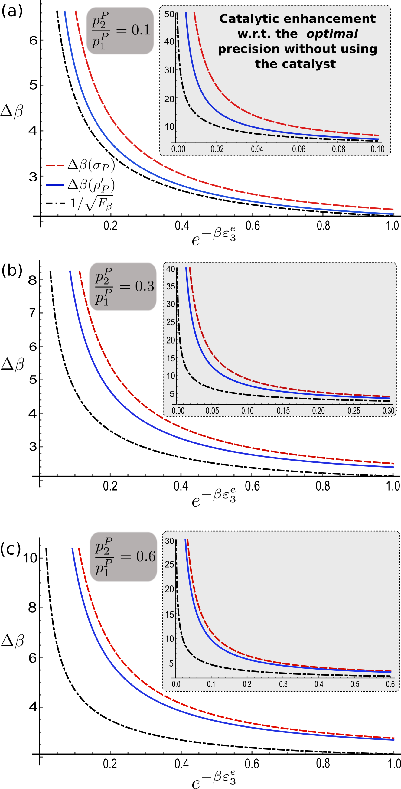
Figure 11 shows the thermometric precision with and without the catalyst, as quantified by the error $\Delta\beta$. The main plots depict this error in the full temperature range $0\leq e^{-\beta\varepsilon_{3}^{e}}\leq 1$, and the insets correspond to the restricted range $e^{-\beta\varepsilon_{3}^{e}}\leq p_{2}^{P}/p_{1}^{P}$, where the state $\rho_{P}\otimes\rho_{e}$ is passive. In all the cases the total transformation is implemented by $UU_{Pe}^{\textrm{opt}}$. The red dashed curves give the error $\Delta\beta(\sigma_{P})$ in Eq. (60), obtained after the application of the swap (64), and the blue solid curves stand for the final error $\Delta\beta(\rho^{\prime}_{P})$, with $\rho^{\prime}_{P}=\textrm{Tr}_{ev}\left(UU_{Pe}^{\textrm{opt}}\rho_{P}\otimes\rho_{e}U_{Pe}^{\textrm{opt}\dagger}U^{\dagger}\right)$. Interestingly, even for $e^{-\beta\varepsilon_{3}^{e}}>p_{2}^{P}/p_{1}^{P}$ the main plots show that the thermometric precision is increased after the catalytic transformation. However, we can be certain that this enhancement surpasses the optimal transformation without the catalyst, only in the interval where $\rho_{P}\otimes\rho_{e}$ is passive. In such a case the initial and final errors obey Eq. (62).

For comparison, the black dash-dotted curves show the thermal Cramer-Rao bound for energy measurements on the environment, which constitutes the minimum (attainable) error using any POVM (positive operator valued measurement). In particular, no probe-based thermometric scheme can surpass this fundamental limit, as illustrated in Fig. 11.

9 Conclusions and outlook

In this paper, we introduced tools for the systematic construction of explicit catalytic transformations on quantum systems of finite size. Size limitations constrain tasks such as cooling using a finite environment or thermometry with a very small probe. In the case of cooling, we showed that the introduction of a catalyst lifts cooling restrictions in two complementary ways: catalysts enable cooling when it is impossible using only the environment, and enhance it when the environment suffices to cool. These results were illustrated with several examples regarding the cooling of a two-level system. In particular, we found that small catalysts such as three-level systems allow maximum cooling in wide temperature ranges. We also demonstrated that to cool a system of any dimension a large enough catalyst and any environment that starts in a non-fully mixed state are sufficient. In addition to the reduction of the system mean energy, its ground population can also be catalytically increased without the need of the environment. Another catalytic advantage was shown in a setup consisting of many qubits prepared in identical states, where a subset of qubits is employed as environment to cool another subset. In this system, we found that it is possible to outperform the cooling achieved through many-body interactions with the environment, by including a two-level catalyst that cools using at most three-body interactions.

For thermometry we studied a simple example where a two-level system extracts temperature information by probing a three-level environment. We established a connection between the minimum estimation error and the notion of passivity for cooling, and then showed that this error can be further reduced if the probe-environment compound undergoes a subsequent interaction with a two-level catalyst. As a matter of fact, this is the smallest physical configuration where a catalyst may improve the thermometric precision achieved through optimal probe-environment interactions. For example, the state of any two-level environment can be fully transferred to a two-level probe, thereby transferring all its Fisher information. In the case of higher-dimensional environments, bounds on the thermometric precision obtained via smaller probes have been recently derived [77]. A natural extension of the results presented here would be to examine if these bounds can be catalytically surpassed. Unveiling further connections between thermometry and passivity is another topic of interest.

Throughout our presentation we have also emphasized the non-unital character of many of the studied transformations, which admit a description in terms of the impossibility to reproduce them through purely classical drivings (see Definition 3 for a formal characterization). Apart from practically motivated non-unital transformations such as cooling, we also showed how catalysts can be used to perform more general transformations of this kind. The identification of other non-unital transformations with interesting applications and their implementation via catalysts could be a subject of future research. The tools provided in the present article could prove very useful in such endeavor.

On the technical side, we list below various questions that remain open:

• Maximum catalytic cooling. The maximum catalytic cooling of a qubit using another qubit as heat sink was studied in Ref. [9]. There, the authors showed that the purity can be increased to a value arbitrarily close to one, if both qubits start in a common state with (von Neumann) entropy smaller than 1/2. In this setting both the catalyst state and the corresponding evolution are unknown. Therefore, it is natural to assume that the dimension of the catalyst and the number of subsystems that compose it enter as (unbounded) variables in the optimization.
  In Sect. VI-A we addressed the same problem, by optimizing over the eigenvalues of a full-rank catalyst state (Appendix I-2) of fixed dimension. Interestingly, we found that for $p_{2}^{c}\lesssim 0.1$ a two-level catalyst suffices to bring the cooled qubit close to its ground state (see Fig. 4(d)). In Appendix L we develop a protocol that extends the scope of this type of optimization. This protocol allows to explore a wider set of global unitaries for catalytic transformations, thereby adding another variable to the optimization task. In particular, we apply it to an example where a two-level system is cooled down through a two-level catalyst and a four-level hot object. After a first maximization with respect to the catalyst eigenvalues, the system energy is reduced by the amount $\Delta\bigl{\langle}H_{c}\bigr{\rangle}=0.033(\varepsilon_{1}^{c}-\varepsilon_{2}^{c})$. Subsequently, the application of the protocol leads to an improved catalytic transformation that yields $\Delta\bigl{\langle}H_{c}\bigr{\rangle}=0.045(\varepsilon_{1}^{c}-\varepsilon_{2}^{c})$.
  Despite the usefulness of the protocol, it is still limited in several aspects. For example, it is restricted to full-rank catalyst states and evolutions given by direct sums of two-level unitaries. Hence, the question of how finite-dimensional catalysts can optimize cooling is completely pertinent. The same question is of course valid for the catalytic optimization of other interesting physical transformations.

• The role of correlations in catalytic transformations. Initial studies on catalysts considered transformations where the catalyst not only remains in its initial state but also does not develop correlations with the rest of the system [2, 1, 15]. Later on, it was shown that these correlations constitute a thermodynamic resource that can be exploited to increase the set of accessible transformations [19] in microscopic thermodynamics. Thanks to this possibility, the so called “second laws” [15] are replaced by the free energy reduction that characterizes the macroscopic second law.
  On the other hand, our results do not assume infinitely large environments, as in Refs. [15] and [19], and focus instead on environments as small as a two-level system. Since the main system is also small, the generation of correlations with the catalyst seems to be a natural prerequisite for the implementation of non-trivial catalytic transformations. Nevertheless, it would be interesting to corroborate this hypothesis, and to study the role played by correlations in our framework and other scenarios where catalysts can yield substantial advantages.

• The role of the catalyst dimension in exact and inexact catalysis. Recently, it was shown that a large class of catalytic transformations are possible without requiring finely tuned catalysts [20]. That is, by employing instead sufficient copies of any catalyst state and allowing a small disturbance in the final state. This relaxation concerning the final state of the catalyst is known as inexact catalysis [16], as opposed to exact catalysis (where the initial and final states must be identical).
  A question that remained open in Ref. [20] was if multi-copy catalysts are essential or if a single-copy catalyst of sufficiently large dimension is equally effective, and numerical evidence in the second direction was given. In this paper we also saw that sufficiently large and single-copy catalysts enable the implementation of cooling and (more general) non-unital transformations, as expressed by Theorem 2. In addition, these results are valid under mild assumptions regarding the initial states of the system and the environment, and for the more stringent regime of exact catalysis. Nonetheless, we also stress that such findings cannot be directly compared with those of Ref. [20], since our approach is based on very different physical constraints such as passivity. With this observation in mind, our results constitute strong evidence of the resourceful character of the catalyst dimension, which could be further explored in other physical scenarios.

Appendices

The following appendices contain all the technical material referred to in the main text. In Appendix A, we derive the stronger form of passivity that leads to Eq. (3) and is applied in the context of cooling. In Appendix B we introduce some notation and describe the class of unitary operations that will be considered subsequently, as well as their relation with the studied transformations. The action of these unitary maps is characterized in Appendix C. In particular, we introduce the key notion of population transfers or “currents”, which forms the basis for the analysis of catalytic transformations. Building upon such a concept, we develop in Appendix D a theoretical framework that contains all the ingredients for the proof of Theorem 1 (Appendix E) and for later results regarding this kind of transformations.

The proofs of Corollary 2 and Theorem 2 are given in Appendix F and Appendix G, respectively. In Appendix H we generalize the catalytic transformations previously studied, by extending the set of unitary operations that allows to implement them. Using the concept of “loop current”, presented in Appendix H, we optimize in Appendix I the catalytic cooling of a two-level system using another two-level system as hot object (cf. Sect. VI-A). The corresponding optimality proof relies on the maximization of the loop current to derive the corresponding maximum cooling. However, such a proof is not restricted to the aforementioned cooling example, and is again applied in the last appendix (Appendix L).

The proof of Theorem 3 and the example of catalytic cooling enhancement presented in Sect. VI-C are developed in Appendix J. In Appendix K we derive a formula for the maximum cooling of a qubit using $k$ identical qubits, which is of great importance for the results of Sect. VII. Finally, we introduce in Appendix L a protocol for the systematic construction of catalytic unitaries that are aimed at increasing the loop current. This protocol is illustrated with an example of catalytic cooling, where it leads to a new transformation with enhanced heat extraction.

Appendix A EXTENDED NOTION OF PASSIVITY

Here we perform the derivation of Eq. (3). To that end, we resort to the fact that the local Hamiltonian $H_{c}$ is also an operator acting on the joint Hilbert space $\mathcal{H}_{c}\otimes\mathcal{H}_{h}$, if written as $H_{c}=H_{c}\otimes\mathbb{I}_{h}$. In this way, we can apply known results [61] to determine when a state that acts on $\mathcal{H}_{c}\otimes\mathcal{H}_{h}$ is passive with respect to $H_{c}$. These results rely on a direct generalization of the standard notion of passivity to arbitrary observables. In our context, this means that, given a state $\rho_{ch}$ and some observable (hermitian operation) $O_{ch}$ that act both on $\mathcal{H}_{c}\otimes\mathcal{H}_{h}$, $\rho_{ch}$ is passive with respect to $O_{ch}$ if and only if $[\rho_{ch},O_{ch}]=0$ and the eigenvalues of $\rho_{ch}$ are non-increasing with respect to those of $O_{ch}$. If $O_{ch}=H_{ch}$ is the Hamiltonian of the joint system described by $\rho_{ch}$ standard passivity is recovered.

Let us see how the aforementioned characterization manifests if $O_{ch}=H_{c}\otimes\mathbb{I}_{h}$ and $\rho_{ch}=\rho_{c}\otimes\rho_{h}$. Since $\mathbb{I}_{h}=\sum_{j=1}^{d_{h}}|j_{h}\rangle\langle j_{h}|$, the eigendecomposition of $H_{c}\otimes\mathbb{I}_{h}$ reads

$$H_{c}\otimes\mathbb{I}_{h}=\sum_{i=1}^{d_{c}}\sum_{j=1}^{d_{h}}\varepsilon_{i}^{c}|i_{c}j_{h}\rangle\langle i_{c}j_{h}|.$$ (72)

First of all, note that $\rho_{c}\otimes\rho_{h}=\sum_{i=1}^{d_{c}}\sum_{j=1}^{d_{h}}p_{i}^{c}p_{j}^{c}|i_{c}j_{h}\rangle\langle i_{c}j_{h}|$ clearly commutes with $H_{c}\otimes\mathbb{I}_{h}$. According to Eq. (72), the eigenvalues of $\rho_{ch}$ are non-increasing with respect to those of $H_{c}\otimes\mathbb{I}_{h}$ if and only if

$$p_{i}^{c}p_{j}^{h}\geq p_{i^{\prime}}^{c}p_{j^{\prime}}^{h}\Leftrightarrow\varepsilon_{i^{\prime}}^{c}\geq\varepsilon_{i}^{c},$$ (73)

for any set of indices $\{i,i^{\prime},j,j^{\prime}\}$.

Assuming (without loss of generality) that the eigenenergies are sorted in non-decreasing order, then $\varepsilon_{i^{\prime}}^{c}\geq\varepsilon_{i}^{c}$ only if $i^{\prime}\geq i+1$. Under this sorting, the equivalence (73) is meaningful only for indices such that $i^{\prime}\geq i+1$. In particular, for $\{i,i^{\prime},j,j^{\prime}\}=\{i,i+1,d_{h},1\}$ it reads: $p_{i}^{c}p_{d_{h}}^{h}\geq p_{i+1}^{c}p_{1}^{h}\Leftrightarrow\varepsilon_{i+1}^{c}\geq\varepsilon_{i}^{c}$. Such statement can be recast as

$$\frac{p_{i}^{c}}{p_{i+1}^{c}}\geq\frac{p_{1}^{h}}{p_{d_{h}}^{h}}\Leftrightarrow\varepsilon_{i+1}^{c}\geq\varepsilon_{i}^{c},$$ (74)

for all $i\in\{1,2,...,d_{c}-1\}$. Since $\frac{p_{1}^{h}}{p_{d_{h}}^{h}}\geq 1$, Eq. (74) tells us that $p_{i}^{c}\geq p_{i+1}^{c}\Leftrightarrow\varepsilon_{i+1}^{c}\geq\varepsilon_{i}^{c}$, i.e. that the eigenvalues of $\rho_{c}$ are non-increasing with respect to those of $H_{c}$. In this way, the passivity of $\rho_{c}\otimes\rho_{h}$ leads to the passivity of $\rho_{c}$, as expected.

On the other hand, Eq. (74) actually coincides with our characterization of passivity (for $\rho_{c}\otimes\rho_{h}$) (3) in the main text. We will show that it is equivalent to the original definition (73), by proving that each side of (74) is equivalent to the corresponding side in (73).

First, the inequalities $\varepsilon_{i+1}^{c}\geq\varepsilon_{i}^{c}$ (for all $i$) are clearly equivalent to the inequalities $\varepsilon_{i^{\prime}}^{c}\geq\varepsilon_{i}^{c}$ (for any $i^{\prime}$ such that $i^{\prime}\geq i+1$). This establishes the equivalence between the r.h.s. of (74) and the r.h.s. of (73). Secondly, $p_{i^{\prime}}^{c}\leq p_{i+1}^{c}$ for all $i^{\prime}\geq i+1$, because $\varepsilon_{i^{\prime}}^{c}\geq\varepsilon_{i+1}^{c}$ for all $i^{\prime}\geq i+1$ and we have seen that $\rho_{c}$ is passive. This allows us to write

$$\frac{p_{i}^{c}}{p_{i^{\prime}}^{c}}\geq\frac{p_{i}^{c}}{p_{i+1}^{c}}\geq\frac{p_{1}^{h}}{p_{d_{h}}^{h}}\geq\frac{p_{j^{\prime}}^{h}}{p_{j}^{h}},$$ (75)

for all $\{i,i^{\prime},j,j^{\prime}\}$ such that $i^{\prime}\geq i+1$. Noting that the inequality connecting the outmost fractions in (75) can be rearranged as $p_{i}^{c}p_{j}^{h}\geq p_{i^{\prime}}^{c}p_{j^{\prime}}^{h}$, we also have the equivalence between the l.h.s. of Eqs. (74) and (73). This concludes the proof.

Appendix B NOTATION AND PRELIMINARIES

Apart from the notation for initial states and their eigendecompositions, described in Sect. II of the main text, we adopt the following conventions.

B.1 Notation for indices

Let $\{1,2,..,n\}$ be a set of indices. Then,

• Any operation over elements labeled by all the indices $i\in\{1,2,...,n\}$ can be written in an explicit or implicit form, being both equivalent. For example, a sum $\sum_{i=1}^{n}a_{i}$ (explicit form), where $a_{i}$ are elements of some set, has the equivalent expression $\sum_{i}a_{i}$ (implicit form). If the operation involves a subset of indices $I\subseteq\{1,2,...,n\}$, this is explicitly written. For example, the sum $\sum_{i\in I}a_{i}$ specifies that only elements $a_{i}$ restricted by the subset $I$ are included.

• The previous convention is also applied to denote sets. For example, the set $\{a_{i}\}_{i}$ is equivalent to the set $\{a_{i}\}_{i=1}^{n}$, and the set $\{a_{i}\}_{i\in I}$ is contained into $\{a_{i}\}_{i}$. In contrast, $\{a_{i}\}$ is the set that contains the single element $a_{i}$.

• Sometimes we will consider operations that ”run” over a non-specific subset of indices. In such a case we add the term “free” to indicate this property. For example, a sum $\sum_{i\textrm{ free}}a_{i}$ is equivalent to a sum $\sum_{i\in I}a_{i}$, where $I$ could be any subset $I\subseteq\{1,2,...,n\}$. The possible subsets $I$ for which the corresponding operation is meaningful will be clear from the context, or explicitly indicated.

• The previous conventions are equally applicable to greek indices. For example, the sum in the eigendecomposition $\rho=\sum_{\psi}p_{\psi}|\psi\rangle\langle\psi|$ runs over all the indices $\psi\in\{1,2,...,d_{c}d_{h}d_{v}\}$ (note that if $\rho$ is not full-rank then $p_{\psi}=0$ for some values of $\psi$).

B.2 Tranformations and unitary operations

All the transformations studied possess an explicit form $\rho\rightarrow\rho^{\prime}=U\rho U^{\dagger}$, where $U$ is a unitary matrix. In this way, the subsystems $x=c,h,v$ undergo associated transformations $\rho_{x}\rightarrow\rho^{\prime}_{x}$, where $\rho_{x}=\textrm{Tr}_{\sim x}\left(\rho\right)$, $\rho^{\prime}_{x}=\textrm{Tr}_{\sim x}\left(\rho^{\prime}\right)$, and $\sim x$ indicates the degrees of freedom different from $x$.

Remark 1. In contrast with primed states (e.g. $\rho^{\prime}$ and $\rho^{\prime}_{x}$), which denote final states, primed labels are used to indicate the specific value taken by an index. For example, the label $i^{\prime}$ indicates that $i$ takes the value $i=i^{\prime}$.

Given a unitary $U$ and a Hilbert subspace $\mathcal{H}_{\textrm{sub}}\subseteq\mathcal{H}$ (where $\mathcal{H}=\mathcal{H}_{c}\otimes\mathcal{H}_{h}\otimes\mathcal{H}_{v}$), we say that $U$ maps $\mathcal{H}_{\textrm{sub}}$ into itself if:

1. $U|\psi\rangle=|\psi\rangle$ for $|\psi\rangle\notin\mathcal{H}_{\textrm{sub}}$.

2. $U|\psi\rangle\in\mathcal{H}_{\textrm{sub}}$ for $|\psi\rangle\in\mathcal{H}_{\textrm{sub}}$.

If $U$ satisfies conditions 1 and 2 we also say that “$U$ acts on $\mathcal{H}_{\textrm{sub}}$”, and write it as $U:\mathcal{H}_{\textrm{sub}}\rightarrow\mathcal{H}_{\textrm{sub}}$. In addition, we term $\mathcal{H}_{\textrm{sub}}$ the “domain subspace” of $U$, as per condition 1.

Definition 4 (two-level unitary). A two-level unitary $U^{(2)}$ is a unitary that acts on a two-dimensional subspace $\textrm{span}\{|\psi\rangle,|\varphi\rangle\}$, where $|\psi\rangle,|\varphi\rangle\in\mathcal{H}$.

Remark 2. If $U$ acts on $\mathcal{H}_{\textrm{sub}}$, conditions 1 and 2 imply that $U$ also acts on any subspace $\mathcal{H}^{\prime}_{\textrm{sub}}$ such that $\mathcal{H}_{\textrm{sub}}\subseteq\mathcal{H}^{\prime}_{\textrm{sub}}$. Moreover, these conditions can be straightforwardly extended to local subspaces. For example, a local unitary $U_{ch}$ acts on a subspace $\mathcal{H}_{\textrm{sub}}\subseteq\mathcal{H}_{c}\otimes\mathcal{H}_{h}$ if 1 and 2 hold, with $|\psi\rangle$ being replaced by $|\psi_{ch}\rangle$.

The unitaries addressed in this work have the form

$$U=\oplus_{\alpha}U_{\alpha},$$ (76)

where $\oplus$ is the direct sum operation. Hence, $U$ is a block-diagonal matrix with blocks $\{U_{\alpha}\}_{\alpha}$. The most basic decomposition of the form (76) is $U=U_{\textrm{cool}}\oplus V_{\textrm{res}}$, where $U_{\textrm{cool}}$ is a cooling unitary and $V_{\textrm{res}}$ is a restoring unitary (see Definitions 1 and 2 in the main text). In this case, $\{U_{\alpha}\}_{\alpha}=\{U_{\textrm{cool}},V_{\textrm{res}}\}$. Later on we will consider other useful decompositions, where $U_{\textrm{cool}}$ and $V_{\textrm{res}}$ are themselves given by block-diagonal matrices.

Appendix C MAIN QUANTITIES FOR THE CHARACTERIZATION OF CATALYTIC TRANSFORMATIONS

C.1 Average variations of observables

Here we derive the general expression for the average variation of an observable (hermitian operator) $O$, given a transformation $\rho\rightarrow\rho^{\prime}=U\rho U^{\dagger}$, where $U$ satisfies Eq. (76). In combination with the notion of population currents, this will allow us to present a description of population variations in the local eigenbases $\{|i_{x=c,v}\rangle\}_{i}$, especially suited for the analysis of catalytic transformations.

To begin with, we express the unitary $U$ in the eigenbasis $\{|\psi\rangle\}_{\psi}$, characteristic of the initial state $\rho$. Specifically, consider the decomposition

$$\rho=\sum_{\alpha}\rho^{(\alpha)},$$ (77)

where the index $\alpha$ labels (disjoint) subsets of eigenstates of $\rho$. Denoting these subsets as $E_{\alpha}$, $\rho^{(\alpha)}$ results from the projection of $\rho$ onto the corresponding subset. Namely, $\rho^{(\alpha)}=\sum_{|\psi\rangle\in E_{\alpha}}|\psi\rangle\langle\psi|\rho\sum_{|\psi\rangle\in E_{\alpha}}|\psi\rangle\langle\psi|$. Each subset $E_{\alpha}$ gives rise to a subspace $\mathcal{H}_{\alpha}=\textrm{span}\{|\psi\rangle\in E_{\alpha}\}$, and $U_{\alpha}$ is a unitary that maps $\mathcal{H}_{\alpha}$ into itself.

The average variation of an observable $O$ is thus given by

$$\Delta\left\langle O\right\rangle=\textrm{Tr}\left[O(U\rho U^{\dagger}-\rho)\right]=\sum_{\alpha}\Delta_{\alpha}\left\langle O\right\rangle,$$ (78)

where

$$\Delta_{\alpha}\left\langle O\right\rangle \equiv\textrm{Tr}\left[O(U_{\alpha}\rho U_{\alpha}^{\dagger}-\rho)\right]$$

$$=\textrm{Tr}\left[O(U_{\alpha}\rho^{(\alpha)}U_{\alpha}^{\dagger}-\rho^{(\alpha)})\right].$$ (79)

The second line in Eq. (79) follows from the fact that $U_{\alpha}|\psi\rangle=|\psi\rangle$ for $|\psi\rangle\notin E_{\alpha}$, and consequently these eigenstates do not contribute to $\Delta_{\alpha}\left\langle O\right\rangle$.

Remark 3. Throughout these appendices we will often replace $\{\alpha\}_{\alpha}$ by a set of indices that are suitable to characterize a particular set of unitaries $\{U_{\alpha}\}_{\alpha}$. As an example, $\alpha$ can be replaced by a pair $\psi,\varphi$ or a related expression, if the set $E_{\alpha}$ only contains the eigenstates $|\psi\rangle$ and $|\varphi\rangle$, i.e. $E_{\alpha}=\{|\psi\rangle,|\varphi\rangle\}$.

C.2 Population variations and currents

If $U_{\alpha}$ is a two-level unitary, it is equivalent to a partial swap $U_{|\psi\rangle\leftrightarrow|\varphi\rangle}$ between the eigenstates $|\psi\rangle$ and $|\varphi\rangle$ that form the set $E_{\alpha}$. Let us express $\alpha$ as $\psi,\varphi$ and $U_{|\psi\rangle\leftrightarrow|\varphi\rangle}$ as $U_{\psi,\varphi}$. Moreover, $\rho^{(\alpha)}$ is equivalent to $\rho^{(\psi,\varphi)}=p_{\psi}|\psi\rangle\langle\psi|+p_{\varphi}|\varphi\rangle\langle\varphi|$. This allows us to characterize the transformation $\rho^{(\psi,\varphi)}\rightarrow U_{\psi,\varphi}\rho^{(\psi,\varphi)}U_{\psi,\varphi}^{\dagger}$ using Eqs. (12) and (13). Denoting the final populations as $p_{\psi}^{\prime}$ and $p_{\varphi}^{\prime}$, we have that

$$U_{\psi,\varphi}\rho^{(\psi,\varphi)}U_{\psi,\varphi}^{\dagger} =p_{\psi}^{\prime}|\psi\rangle\langle\psi|+p_{\varphi}^{\prime}|\varphi\rangle\langle\varphi|$$

$$\quad+\sqrt{(1-r)r}\left(|\psi\rangle\langle\varphi|+|\varphi\rangle\langle\psi|\right),$$ (80)

where $p_{\psi}^{\prime}=p_{\psi}+r(p_{\varphi}-p_{\psi})$ is given in (14) and $p_{\varphi}^{\prime}=p_{\psi}+p_{\varphi}-p_{\psi}^{\prime}$ .

The observable $O_{k^{\prime}}\equiv|k_{v}^{\prime}\rangle\langle k_{v}^{\prime}|$ characterizes the catalyst population $\left\langle|k_{v}^{\prime}\rangle\langle k_{v}^{\prime}|\right\rangle$. From Eq. (80) we obtain:

$$\textrm{Tr}\left[O_{k^{\prime}}U_{\psi,\varphi}\rho^{(\psi,\varphi)}U_{\psi,\varphi}^{\dagger}\right]=p_{\psi}^{\prime}|\langle k_{v}^{\prime}|\psi\rangle|^{2}+p_{\varphi}^{\prime}|\langle k_{v}^{\prime}|\varphi\rangle|^{2}.$$ (81)

Hence,

$$\Delta_{\psi,\varphi}\left\langle O_{k^{\prime}}\right\rangle =\textrm{Tr}\left[O_{k^{\prime}}\left(U_{\psi,\varphi}\rho^{(\psi,\varphi)}U_{\psi,\varphi}^{\dagger}-\rho^{(\psi,\varphi)}\right)\right]$$

$$=\left(p_{\psi}^{\prime}-p_{\psi}\right)|\langle k_{v}^{\prime}|\psi\rangle|^{2}+\left(p_{\varphi}^{\prime}-p_{\varphi}\right)|\langle k_{v}^{\prime}|\varphi\rangle|^{2}$$

$$=r(p_{\varphi}-p_{\psi})\left[|\langle k_{v}^{\prime}|\psi\rangle|^{2}-|\langle k_{v}^{\prime}|\varphi\rangle|^{2}\right]$$

$$=J_{|\varphi\rangle\rightarrow|\psi\rangle}\left[|\langle k_{v}^{\prime}|\psi\rangle|^{2}-|\langle k_{v}^{\prime}|\varphi\rangle|^{2}\right],$$ (82)

where the third line follows from the definition of the current $J_{|\varphi\rangle\rightarrow|\psi\rangle}$ (cf. Eq. (15)).

Remark 4. In this work, the unitaries that lead to catalytic transformations are composed of two-level unitaries $U_{|\psi\rangle\leftrightarrow|\varphi\rangle}$ such that $\textrm{Tr}_{ch}|\psi\rangle\langle\varphi|=\textrm{Tr}_{v}|\psi\rangle\langle\varphi|=0$. Accordingly, $|\psi\rangle=|\psi_{ch}k^{\prime}_{v}\rangle$ and $|\varphi\rangle=|\varphi_{ch}k_{v}^{\prime\prime}\rangle$, where $|\psi_{ch}\rangle$, $|\varphi_{ch}\rangle$ are different eigenstates of $\rho_{ch}$ and $|k^{\prime}_{v}\rangle$, $|k_{v}^{\prime\prime}\rangle$ are different eigenstates of $\rho_{v}$.

A consequence of Remark 4 is that if $|\langle k_{v}^{\prime}|\psi\rangle|=1$ then $|\langle k_{v}^{\prime}|\varphi\rangle|=0$ and vice versa. Accordingly, either $\Delta_{\psi,\varphi}\left\langle O_{k^{\prime}}\right\rangle=J_{|\varphi\rangle\rightarrow|\psi\rangle}$ (if $|\langle k_{v}^{\prime}|\psi\rangle|=1$), or $\Delta_{\psi,\varphi}\left\langle O_{k^{\prime}}\right\rangle=-J_{|\varphi\rangle\rightarrow|\psi\rangle}$ (if $|\langle k_{v}^{\prime}|\varphi\rangle|=1$). Since $J_{|\varphi\rangle\rightarrow|\psi\rangle}=-J_{|\psi\rangle\rightarrow|\varphi\rangle}$ (cf. Eq. (15)), we can rewrite Eq. (82) as

$$\Delta_{\psi,\varphi}\left\langle O_{k^{\prime}}\right\rangle=\begin{cases}\begin{array}[]{c}J_{|\varphi\rangle\rightarrow|\psi\rangle},\textrm{ if }|\langle k_{v}^{\prime}|\psi\rangle|=1,\\ J_{|\psi\rangle\rightarrow|\varphi\rangle},\textrm{ if }|\langle k_{v}^{\prime}|\varphi\rangle|=1,\\ 0,\textrm{ otherwise.}\end{array}\end{cases}$$ (83)

Consider now a set of partial swaps $\{U_{\psi,\varphi}\}_{\psi,\varphi\textrm{ free}}$ acting on orthogonal subspaces $\mathcal{H}_{\psi,\varphi}=\textrm{span}\{|\psi\rangle,|\varphi\rangle\}$. Taking into account Eq. (78), for $U=\oplus_{\psi,\varphi\textrm{ free}}U_{\psi,\varphi}$ we obtain:

$$\Delta\left\langle O_{k^{\prime}}\right\rangle =\textrm{Tr}\left[O_{k^{\prime}}\left(U\rho U^{\dagger}-\rho\right)\right]$$

$$=\sum_{\psi,\varphi\textrm{ free}}\Delta_{\psi,\varphi}\left\langle O_{k^{\prime}}\right\rangle,$$ (84)

where $\Delta_{\psi,\varphi}\left\langle O_{k^{\prime}}\right\rangle$ obeys Eq. (83).

C.3 Diagonal form of the final catalyst state

Before moving forward, it is important to point out a fact that underpins all our forthcoming analysis on catalytic transformations. Based on Proposition 2, we can fully characterize catalytic transformations in terms of the populations in the eigenbasis of the initial state $\rho_{v}$.

Proposition 2. For any unitary $U=\oplus_{\psi,\varphi\textrm{ free}}U_{\psi,\varphi}$ where each pair of eigenstates $|\psi\rangle$ and $|\varphi\rangle$ adhere to Remark 4, the catalyst state $\rho^{\prime}_{v}=\textrm{Tr}_{ch}\left(U\rho U^{\dagger}\right)$ is diagonal in the eigenbasis of the initial state $\rho_{v}$. Moreover, this is true for any state $\rho=\rho_{ch}\otimes\rho_{v}$, irrespective of the form of $\rho_{ch}$.

Proof. The action of direct sum $U=\oplus_{\psi,\varphi\textrm{ free}}U_{\psi,\varphi}$ on $\rho$ is given in terms of the action of each $U_{\psi,\varphi}$ on the corresponding projection. That is,

$$U\rho U^{\dagger}=\sum_{\psi,\varphi\textrm{ free}}U_{\psi,\varphi}\rho^{(\psi,\varphi)}U_{\psi,\varphi}^{\dagger},$$ (85)

with $U_{\psi,\varphi}\rho^{(\psi,\varphi)}U_{\psi,\varphi}^{\dagger}$ given in Eq. (80). Keeping in mind Remark 4, we have that $\textrm{Tr}_{ch}|\psi\rangle\langle\varphi|=0$ for any pair $|\psi\rangle,|\varphi\rangle$. Therefore, (80) and (85) yields the state $\textrm{Tr}_{ch}\left(U\rho U^{\dagger}\right)=\sum_{\psi,\varphi\textrm{ free}}\left(p_{\psi}^{\prime}\textrm{Tr}_{ch}|\psi\rangle\langle\psi|+p_{\varphi}^{\prime}\textrm{Tr}_{ch}|\varphi\rangle\langle\varphi|\right)$, which is diagonal in the eigenbasis of $\rho_{v}$.

Appendix D LOOPS AND CATALYTIC TRANSFORMATIONS

For global eigenstates $|\psi\rangle=|i_{c}^{\prime}j_{h}^{\prime}k_{v}^{\prime}\rangle$ and $|\varphi\rangle=|i_{c}^{\prime\prime}j_{h}^{\prime\prime}k_{v}^{\prime\prime}\rangle$, a two-level unitary $U_{\psi,\varphi}$ generates local currents between all the pairs of local eigenstates. This is a consequence of the fact that $\textrm{span}\{|\psi\rangle,|\varphi\rangle\}$ is contained into $\textrm{span}\{|i_{c}^{\prime}\rangle,|i_{c}^{\prime\prime}\rangle\}\otimes\textrm{span}\{|j_{h}^{\prime}\rangle,|j_{h}^{\prime\prime}\rangle\}\otimes\textrm{span}\{|k_{v}^{\prime}\rangle,|k_{v}^{\prime\prime}\rangle\}$, and therefore $U_{\psi,\varphi}$ maps the later subspace into itself (cf. Remark 2). More specifically, this implies that $\Delta_{\psi,\varphi}\left\langle|i_{c}^{\prime}\rangle\langle i_{c}^{\prime}|\right\rangle=-\Delta_{\psi,\varphi}\left\langle|i_{c}^{\prime\prime}\rangle\langle i_{c}^{\prime\prime}|\right\rangle$, $\Delta_{\psi,\varphi}\left\langle|j_{h}^{\prime}\rangle\langle j_{h}^{\prime}|\right\rangle=-\Delta_{\psi,\varphi}\left\langle|j_{h}^{\prime\prime}\rangle\langle k_{h}^{\prime\prime}|\right\rangle$, and $\Delta_{\psi,\varphi}\left\langle|k_{v}^{\prime}\rangle\langle k_{v}^{\prime}|\right\rangle=-\Delta_{\psi,\varphi}\left\langle|k_{v}^{\prime\prime}\rangle\langle k_{v}^{\prime\prime}|\right\rangle$. Therefore, the variation $\Delta_{\psi,\varphi}\left\langle|k_{v}^{\prime}\rangle\langle k_{v}^{\prime}|\right\rangle$ is associated with a population transfer from $|k_{v}^{\prime\prime}\rangle$ to $|k_{v}^{\prime}\rangle$, described by a local current $J_{|k_{v}^{\prime\prime}\rangle\rightarrow|k_{v}^{\prime}\rangle}$. Likewise, the population variations $\Delta_{\psi,\varphi}\left\langle|i_{c}^{\prime}\rangle\langle i_{c}^{\prime}|\right\rangle$ and $\Delta_{\psi,\varphi}\left\langle|j_{h}^{\prime}\rangle\langle j_{h}^{\prime}|\right\rangle$ are also associated with local currents $J_{|i_{c}^{\prime\prime}\rangle\rightarrow|i_{c}^{\prime}\rangle}$ and $J_{|j_{h}^{\prime\prime}\rangle\rightarrow|j_{h}^{\prime}\rangle}$, respectively.

The same calculations that allowed us to derive Eq. (83) can be straightforwardly applied to express $\Delta_{\psi,\varphi}\left\langle|i_{c}^{\prime}\rangle\langle i_{c}^{\prime}|\right\rangle$ and $\Delta_{\psi,\varphi}\left\langle|j_{h}^{\prime}\rangle\langle j_{h}^{\prime}|\right\rangle$ in terms of the global current $J_{|\varphi\rangle\rightarrow|\psi\rangle}$. In this way, we have that:

$$\Delta_{\psi,\varphi}\left\langle O_{k^{\prime}}\right\rangle =J_{|k_{v}^{\prime\prime}\rangle\rightarrow|k_{v}^{\prime}\rangle}=J_{|\varphi\rangle\rightarrow|\psi\rangle},$$ (86)

$$\Delta_{\psi,\varphi}\left\langle|i_{c}^{\prime}\rangle\langle i_{c}^{\prime}|\right\rangle =J_{|i_{c}^{\prime\prime}\rangle\rightarrow|i_{c}^{\prime}\rangle}=J_{|\varphi\rangle\rightarrow|\psi\rangle},$$ (87)

$$\Delta_{\psi,\varphi}\left\langle|j_{h}^{\prime}\rangle\langle j_{h}^{\prime}|\right\rangle =J_{|j_{h}^{\prime\prime}\rangle\rightarrow|j_{h}^{\prime}\rangle}=J_{|\varphi\rangle\rightarrow|\psi\rangle},$$ (88)

where we have reserved the simplified notation $O_{k^{\prime}}$ for the projector $|k_{v}^{\prime}\rangle\langle k_{v}^{\prime}|$, as Eq. (86) will be the most utilized among Eqs. (86)-(88).

These equations provide the equalities in Eqs. (17)-(19) of the main text. The upper bounds in (17)-(19) follow by realizing that $J_{|\varphi\rangle\rightarrow|\psi\rangle}$ is maximum or minimum for $r=1$, in which case $J_{|\varphi\rangle\rightarrow|\psi\rangle}=\mathcal{J}_{|\varphi\rangle\rightarrow|\psi\rangle}$.

Remark 5. A local current is essentially a population transfer between a pair of local eigenstates, and it is not restricted to two-level unitaries $U_{\psi,\varphi}$. For example, any unitary $U$ that acts on a subspace $\mathcal{H}_{c}\otimes\mathcal{H}_{h}\otimes\textrm{span}\{|k_{v}^{\prime\prime}\rangle,|k_{v}^{\prime}\rangle\}$ generates a local current $J_{|k_{v}^{\prime\prime}\rangle\rightarrow|k_{v}^{\prime}\rangle}=\Delta\bigl{\langle}O_{k^{\prime}}\bigr{\rangle}=-\Delta\bigl{\langle}O_{k_{v}^{\prime\prime}}\bigr{\rangle}$. Likewise, any unitary $U$ that acts on a subspace $\textrm{span}\{|i_{c}^{\prime\prime}\rangle,|i_{c}^{\prime}\rangle\}\otimes\mathcal{H}_{h}\otimes\mathcal{H}_{v}$ generates a local current $J_{|i_{c}^{\prime\prime}\rangle\rightarrow|i_{c}^{\prime}\rangle}=\Delta\bigl{\langle}|i^{\prime}_{c}\rangle\langle i^{\prime}_{c}|\bigr{\rangle}-\Delta\bigl{\langle}|i_{c}^{\prime\prime}\rangle\langle i_{c}^{\prime\prime}|\bigr{\rangle}$.

In particular, consider a set of local unitaries $\{U_{\psi,\varphi}\}_{\psi,\varphi\textrm{ free}}$, such that $U_{\psi,\varphi}$ acts on the subspace $\textrm{span}\{|\psi_{ch}k_{v}^{\prime}\rangle,|\varphi_{ch}k_{v}^{\prime\prime}\rangle\}$ (where $\psi$ and $\varphi$ are fixed). Since $\oplus_{\psi,\varphi\textrm{ free}}U_{\psi,\varphi}$ acts on $\mathcal{H}_{c}\otimes\mathcal{H}_{h}\otimes\textrm{span}\{|k_{v}^{\prime\prime}\rangle,|k_{v}^{\prime}\rangle\}$, as per Remark 2, it generates a current $J_{|k_{v}^{\prime\prime}\rangle\rightarrow|k_{v}^{\prime}\rangle}$ (Remark 5). Using Eqs. (84) and (86), we have that

$$J_{|k_{v}^{\prime\prime}\rangle\rightarrow|k_{v}^{\prime}\rangle}=\sum_{\psi,\varphi\textrm{ free}}J_{|\varphi\rangle\rightarrow|\psi\rangle}.$$ (89)

Moreover, we can define the “swap local current”

$$\mathcal{J}_{|k_{v}^{\prime\prime}\rangle\rightarrow|k_{v}^{\prime}\rangle}\equiv\sum_{\psi,\varphi\textrm{ free}}\mathcal{J}_{|\varphi\rangle\rightarrow|\psi\rangle},$$ (90)

which is produced by the direct sum of swaps $\oplus_{\psi,\varphi\textrm{ free}}\mathcal{U}_{\psi,\varphi}$. The current $J_{|k_{v}^{\prime\prime}\rangle\rightarrow|k_{v}^{\prime}\rangle}$ and the corresponding swap current $\mathcal{J}_{|k_{v}^{\prime\prime}\rangle\rightarrow|k_{v}^{\prime}\rangle}$ in (19) can be recovered from (89) and (90), when the direct sums $\oplus_{\psi,\varphi\textrm{ free}}U_{\psi,\varphi}$ and $\oplus_{\psi,\varphi\textrm{ free}}\mathcal{U}_{\psi,\varphi}$ reduce to a single two-level unitary.

Equipped with the general concept of local current characterized in Remark 5, we can now introduce the most important element for the analysis of catalytic transformations. Namely, the “loop”. To define this element, we must first define the related concept of “chain”.

Definition 5 (chain). Let $\{k^{(m)}\}_{m=1}^{M}$ be a set of indices, where $k^{(m)}\in\{1,2,...,d_{v}\}$, and let $J_{|k_{v}^{(m+1)}\rangle\rightarrow|k_{v}^{(m)}\rangle}$ be a local current generated by a unitary that acts on $\mathcal{H}_{c}\otimes\mathcal{H}_{h}\otimes\textrm{span}\{|k_{v}^{(m+1)}\rangle,|k_{v}^{(m)}\rangle\}$. A chain is a set $\{J_{|k_{v}^{(m+1)}\rangle\rightarrow|k_{v}^{(m)}\rangle}\}_{m=1}^{M-1}$, where $J_{|k_{v}^{(m+1)}\rangle\rightarrow|k_{v}^{(m)}\rangle}>0$ for $1\leq m\leq M-1$.

Intuitively, the “direction” pointed out by the currents in a chain leads us from the eigenstate $|k_{v}^{(M)}\rangle$ towards the eigenstate $|k_{v}^{(1)}\rangle$, as illustrated in Fig. 12 . To capture this intuition, we employ the notation $\mathbf{ch}_{|k_{v}^{(M)}\rangle\rightarrow|k_{v}^{(1)}\rangle}$, and refer to $|k_{v}^{(M)}\rangle$ and $|k_{v}^{(1)}\rangle$ (or $k_{v}^{(M)}$ and $k_{v}^{(1)}$ in the $\textrm{ln}(p^{ch})\times\textrm{ln}(p^{v})$ diagram) as the “origin” and the “end” of the chain, respectively.

Definition 6 (loop). A loop is a set of currents $\mathbf{ch}_{|k_{v}^{(M)}\rangle\rightarrow|k_{v}^{(1)}\rangle}\cup\{J_{|k_{v}^{(1)}\rangle\rightarrow|k_{v}^{(M)}\rangle}\}$, where $J_{|k_{v}^{(1)}\rangle\rightarrow|k_{v}^{(M)}\rangle}>0$. This set can be described using the equivalent notations $\mathbf{loop}_{|k_{v}^{(M)}\rangle\rightarrow|k_{v}^{(M)}\rangle}=\mathbf{loop}_{|k_{v}^{(1)}\rangle\rightarrow|k_{v}^{(1)}\rangle}$. Moreover, it can be seen as a “closed chain”, where $|k_{v}^{(M)}\rangle$ and $|k_{v}^{(1)}\rangle$ play both the roles of origin and end.

Figure 12: Two examples of chains $\mathbf{ch}_{|(l^{\prime}+1)_{v}\rangle\rightarrow|l_{v}\rangle}$ and associated global currents in the $\textrm{ln}(p^{ch})\times\textrm{ln}(p^{v})$ diagram. By including a positive current $J_{|l_{v}\rangle\rightarrow|(l^{\prime}+1)_{v}\rangle}$, both chains can from a loop $\mathbf{loop}_{|l_{v}\rangle\rightarrow|l_{v}\rangle}$ (see e.g. Fig. 3(a)). (a) Elemental chain (see Definition 7) generated by a unitary $\oplus_{k=k^{(1)}}^{k^{(5)}-1}V_{k}$ , where $V_{k}=V_{|n_{ch}(k+1)_{v}\rangle\leftrightarrow|N_{ch}k_{v}\rangle}$ and $\{k^{(1)},k^{(5)}\}=\{l,l^{\prime}+1\}$. The local currents in this kind of chain connect all the consecutive rows from $l^{\prime}+1$ to $l$. (b) Another chain with the same origin ($l^{\prime}+1$) and end ($l$) of the elemental chain. Here, the end is reached by replacing the global current $J_{|n_{ch}k_{v}^{(2)}\rangle\rightarrow|N_{ch}k_{v}^{(1)}\rangle}$(arrow inside the darker rectangle) in (a), by $J_{|n_{ch}k_{v}^{\prime(3)}\rangle\rightarrow|N_{ch}k_{v}^{\prime(2)}\rangle}$ (dashed green arrow) and $J_{|n_{ch}k_{v}^{\prime(2)}\rangle\rightarrow|n_{ch}k_{v}^{\prime(1)}\rangle}$ (black arrow). Since the local current $J_{|k_{v}^{\prime(3)}\rangle\rightarrow|k_{v}^{\prime(2)}\rangle}$ does not connect consecutive rows, this chain is not elemental.

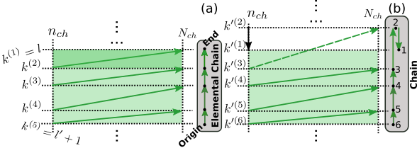
D.1 Loop generation via a direct sum of unitaries

In Fig. 12 we apply the $\textrm{ln}(p^{ch})\times\textrm{ln}(p^{v})$ diagram to illustrate two sets of currents $\{J_{|k_{v}^{(m+1)}\rangle\rightarrow|k_{v}^{(m)}\rangle}\}_{m=1}^{M-1}$ that give rise to chains $\mathbf{ch}_{|(l^{\prime}+1)_{v}\rangle\rightarrow|l_{v}\rangle}$ with a common origin $l^{\prime}+1$ and end $l$. The chain in (a) was already illustrated in Fig. 3, and is an example of the following set:

Definition 7 (elemental chain). An elemental chain is a chain $\mathbf{ch}_{|k^{(M)}\rangle\rightarrow|k^{(1)}\rangle}=\{J_{|(k+1)_{v}\rangle\rightarrow|k_{v}\rangle}\}_{k=k^{(1)}}^{k^{(M)}-1}$, where all the currents connect consecutive eigenstates $\{|k_{v}\rangle\}_{k=k^{(1)}}^{k^{(M)}}$, and no eigenstate $|k_{v}\rangle$ with $k\leq k^{(1)}-1$ or $k\geq k^{(M)}+1$ is connected.

Figure 12(b) shows that a chain $\mathbf{ch}_{|(l^{\prime}+1)_{v}\rangle\rightarrow|l_{v}\rangle}$ is not restricted to its elemental version. Taking this into account, the purpose of the present section is twofold. On the one hand, we will set necessary conditions for the generation of a loop through a proper (direct) sum of unitaries. On the other hand, we will show that any chain $\mathbf{ch}_{|k_{v}^{(M)}\rangle\rightarrow|k_{v}^{(1)}\rangle}$ in this loop can exist only if the elemental chain exists. These results are fundamental to characterize the existence of catalytic transformations in our framework.

D.1.1 Equations for catalyst population variations

Consider a set of subspaces $\{\mathcal{H}_{k^{(m)}}\}_{m=1}^{M}$, such that such that

$$\mathcal{H}_{k^{(m)}}\equiv\textrm{span}\{|\psi_{ch}\rangle\}_{\psi=n}^{N}\otimes\textrm{span}\{|k_{v}^{(m+1)}\rangle,|k_{v}^{(m)}\rangle\}$$ (91)

for $m\in\{1,2,...,M\}$, where we introduce a periodic boundary condition $k^{(M+1)}=k^{(1)}$. This periodicity condition implies that $\mathcal{H}_{k^{(M)}}=\mathcal{H}_{c}\otimes\mathcal{H}_{h}\otimes\textrm{span}\{|k_{v}^{(1)}\rangle,|k_{v}^{(M)}\rangle\}.$ Moreover, let $\{V_{k^{(m)}}\}_{m=1}^{M-1}$ and $U_{k^{(M)}}$ be unitaries whose domain subspaces are $\{\mathcal{H}_{k^{(m)}}\}_{m=1}^{M-1}$ and $\mathcal{H}_{k^{(M)}}$, respectively:

$$V_{k^{(m)}} :\mathcal{H}_{k^{(m)}}\rightarrow\mathcal{H}_{k^{(m)}},\textrm{ for }m\in\{1,2,...,M-1\},$$

$$U_{k^{(M)}} :\mathcal{H}_{k^{(M)}}\rightarrow\mathcal{H}_{k^{(M)}}.$$ (92)

Importantly, both $V_{k^{(m)}}$ and $U_{k^{(M)}}$ do not have to be two-level unitaries.

Remark 6. For the sake of brevity, in the remainder of these appendices the indices $n$ and $N$ in the subspaces $\{\mathcal{H}_{k^{(m)}}\}_{m=1}^{M}$ will be left implicit.

Our goal now is to set the stage for the generation of a loop via a direct sum:

$$U=U_{k^{(M)}}\oplus\left(\oplus_{m=1}^{M-1}V_{k^{(m)}}\right).$$ (93)

Taking into account Remark 3, let us make the correspondence $\{\alpha\}_{\alpha}=\{k^{(m)}\}_{m=1}^{M}$. In this way, the variation of the catalyst population $\left\langle O_{k^{(m^{\prime})}}\right\rangle=\left\langle|k_{v}^{(m^{\prime})}\rangle\langle k_{v}^{(m^{\prime})}|\right\rangle$ reads (cf. (78))

$$\Delta\left\langle O_{k^{(m^{\prime})}}\right\rangle=\sum_{m=1}^{M}\Delta_{k^{(m)}}\left\langle O_{k^{(m^{\prime})}}\right\rangle,$$ (94)

where (cf. (79))

$$\Delta_{k^{(M)}}\left\langle O_{k^{(m^{\prime})}}\right\rangle =\textrm{Tr}\left[O_{k^{(m^{\prime})}}\left(U_{k^{(M)}}\rho^{(k^{(M)})}U_{k^{(M)}}^{\dagger}\right.\right.$$

$$\quad\left.\left.-\rho^{(k^{(M)})}\right)\right]$$ (95)

and

$$\Delta_{k^{(m)}}\left\langle O_{k^{(m^{\prime})}}\right\rangle =\textrm{Tr}\left[O_{k^{(m^{\prime})}}\left(V_{k^{(m)}}\rho^{(k^{(m)})}V_{k^{(m)}}^{\dagger}\right.\right.$$

$$\quad\left.\left.-\rho^{(k^{(m)})}\right)\right]$$ (96)

for $1\leq m\leq M-1$.

Since the supports of $V_{k^{(m)}}\rho^{(k^{(m)})}V_{k^{(m)}}^{\dagger}$ and $\rho^{(k^{(m)})}$ are both contained into $\mathcal{H}_{k^{(m)}}$, $\Delta_{k^{(m)}}\left\langle O_{k^{(m^{\prime})}}\right\rangle$ can be different from zero only if $\mathcal{H}_{k^{(m)}}$ contains states with a non-null probability to measure $|k_{v}^{(m^{\prime})}\rangle$. Moreover, the same argument applies to the variation $\Delta_{k^{(M)}}\left\langle O_{k^{(m^{\prime})}}\right\rangle$. Following the definition (91), we thus have that only $\mathcal{H}_{k^{(m^{\prime})}}$ and $\mathcal{H}_{k^{(m^{\prime}-1)}}$ can provide a non-null contribution to $\Delta\left\langle O_{k^{(m^{\prime})}}\right\rangle$ in Eq. (94). Using the periodic boundary condition $k^{(M+1)}=k^{(1)}$ and setting also $k^{(0)}\equiv k^{(M)}$, we can write $\Delta\left\langle O_{k^{(m^{\prime})}}\right\rangle$ in the compact manner:

$$\Delta\left\langle O_{k^{(m^{\prime})}}\right\rangle =\Delta_{k^{(m^{\prime}-1)}}\left\langle O_{k^{(m^{\prime})}}\right\rangle+\Delta_{k^{(m^{\prime})}}\left\langle O_{k^{(m^{\prime})}}\right\rangle$$

$$=J_{|k_{v}^{(m^{\prime}-1)}\rangle\rightarrow|k_{v}^{(m^{\prime})}\rangle}+J_{|k_{v}^{(m^{\prime}+1)}\rangle\rightarrow|k_{v}^{(m^{\prime})}\rangle}$$

$$=J_{|k_{v}^{(m^{\prime}-1)}\rangle\rightarrow|k_{v}^{(m^{\prime})}\rangle}-{\color[rgb]{1,0,0}\definecolor[named]{pgfstrokecolor}{rgb}{1,0,0}{\normalcolor J_{|k_{v}^{(m^{\prime})}\rangle\rightarrow|k_{v}^{(m^{\prime}+1)}\rangle}}},$$ (97)

for $1\leq m^{\prime}\leq M$. In the second line of Eq. (97), we have resorted to Remark 5 to express the average variations in the first line as local currents.

The currents appearing in Eq. (97) form the set $\{J_{|k_{v}^{(m+1)}\rangle\rightarrow|k_{v}^{(m)}\rangle}\}_{m=1}^{M-1}\cup\{J_{|k_{v}^{(1)}\rangle\rightarrow|k_{v}^{(M)}\rangle}\}$. If all these currents have the same magnitude, Eqs. (97) implies that $\Delta\left\langle O_{k^{(m^{\prime})}}\right\rangle=0$ for $m^{\prime}\in\{1,2,...,M\}$. For $k^{(m^{\prime})}$ such that $m^{\prime}\notin\{1,2,...,M\}$, the populations $\bigl{\langle}O_{k^{(m^{\prime})}}\bigr{\rangle}$ remain trivially unchanged under the action of $U$ (Eq. (93)), since it acts on a subspace that does not contain any state with a non-null probability to measure $O_{k^{(m^{\prime})}}$. This leads us to the following observation:

Remark 7. If $U_{k^{(M)}}$ generates a positive current $J_{|k_{v}^{(1)}\rangle\rightarrow|k_{v}^{(M)}\rangle}>0$, the transformation $\rho\rightarrow\rho^{\prime}=U\rho U^{\dagger}$ (where $U$ satisfies (93)) is catalytic only if $U$ generates a uniform loop $\mathbf{ch}_{|k_{v}^{(M)}\rangle\rightarrow|k_{v}^{(1)}\rangle}\cup\{J_{|k_{v}^{(1)}\rangle\rightarrow|k_{v}^{(M)}\rangle}\}$, defined as a loop where the currents in the chain $\mathbf{ch}_{|k_{v}^{(M)}\rangle\rightarrow|k_{v}^{(1)}\rangle}$ satisfy $J_{|k_{v}^{(m+1)}\rangle\rightarrow|k_{v}^{(m)}\rangle}=J_{|k_{v}^{(1)}\rangle\rightarrow|k_{v}^{(M)}\rangle}$. If $\rho^{\prime}_{v}=\textrm{Tr}_{ch}\rho^{\prime}$ is diagonal in the eigenbasis of $\rho_{v}$, a uniform loop also guarantees that $\rho\rightarrow\rho^{\prime}=U\rho U^{\dagger}$ is catalytic.

D.1.2 Conditions for the generation of a uniform loop

In Lemma 1 we provide necessary and sufficient conditions for the generation of a uniform loop. To that end, we introduce the following definition, which is yet another generalization of passivity. As can be readily seen from Eq. (98), it recovers usual passivity with respect to an arbitrary observable if $\mathcal{H}_{\alpha^{\prime}}=\mathcal{H}$.

Definition 8 (passivity within a Hilbert subspace). Let $\{U_{\alpha^{\prime}}\}_{U_{\alpha^{\prime}}}=\{U:U\textrm{ acts on }\mathcal{\mathcal{H}}_{\alpha^{\prime}}\}$ be the set of all the unitaries that map a fixed subspace $\mathcal{H}_{\alpha^{\prime}}\subseteq\mathcal{H}$ into itself (not to confuse with $\{U_{\alpha}\}_{\alpha}$, which denotes a set where each $U_{\alpha}$ acts on a different $\mathcal{H}_{\alpha}$). We say that a state $\rho$ is passive with respect to the pair $\{O,\mathcal{H}_{\alpha^{\prime}}\}$, where $O$ is a general observable (global or local), iff $\textrm{{Tr}}\left(OU_{\alpha^{\prime}}\rho U_{\alpha^{\prime}}^{\dagger}\right)\geq\textrm{{Tr}}\left(O\rho\right)$ for any $U_{\alpha^{\prime}}\in\{U_{\alpha^{\prime}}\}_{U_{\alpha^{\prime}}}$.

The previous definition can be conveniently recast by decomposing $\rho$ as $\rho=\rho^{(\alpha^{\prime})}+\rho^{(\sim\alpha^{\prime})}$ (cf. Eq. (77)), where $\rho^{(\sim\alpha^{\prime})}=\sum_{|\psi\rangle\notin E_{\alpha^{\prime}}}|\psi\rangle\langle\psi|\rho\sum_{|\psi\rangle\notin E_{\alpha^{\prime}}}|\psi\rangle\langle\psi|$. Since $U_{\alpha^{\prime}}|\psi\rangle=|\psi\rangle$ for $|\psi\rangle\notin E_{\alpha^{\prime}}$, $\textrm{Tr}\left(OU_{\alpha^{\prime}}\rho U_{\alpha^{\prime}}^{\dagger}\right)=\textrm{Tr}\left(OU_{\alpha^{\prime}}\rho^{(\alpha^{\prime})}U_{\alpha^{\prime}}^{\dagger}\right)+\textrm{Tr}\left(O\rho^{(\sim\alpha^{\prime})}\right)$. Accordingly, $\rho$ is passive with respect to $\{O,\mathcal{H}_{\alpha^{\prime}}\}$ iff, for any $U_{\alpha^{\prime}}$,

$$\textrm{Tr}\left[O\left(U_{\alpha^{\prime}}\varrho^{(\alpha^{\prime})}U_{\alpha^{\prime}}^{\dagger}\right)\right]\geq\textrm{Tr}\left[O\left(\varrho^{(\alpha^{\prime})}\right)\right],$$ (98)

where $\varrho^{(\alpha^{\prime})}=\rho^{(\alpha^{\prime})}/\textrm{Tr}\left(\rho^{(\alpha^{\prime})}\right)$ is the normalized version of $\varrho^{(\alpha^{\prime})}$.

Note also that a necessary condition for Eq. (98) is that $[O,\varrho^{(\alpha^{\prime})}]=0$. Therefore, $O$ must have an eigendecomposition $O=\sum_{\psi}o_{\psi}|\psi\rangle\langle\psi|$. Given that the supports of $\varrho^{(\alpha^{\prime})}$ and $U_{\alpha^{\prime}}\varrho^{(\alpha^{\prime})}U_{\alpha^{\prime}}^{\dagger}$ are both contained in $E_{\alpha^{\prime}}$, we can replace $O$ by $\sum_{\psi:|\psi\rangle\in E_{\alpha^{\prime}}}o_{\psi}|\psi\rangle\langle\psi|$ in Eq. (98) (as the average values over $\sum_{\psi:|\psi\rangle\notin E_{\alpha^{\prime}}}o_{\psi}|\psi\rangle\langle\psi|$ are null). Hence, all the relevant operators in (98) have eigenstates that belong to $\mathcal{H}_{\alpha^{\prime}}$, and we can apply standard passivity considering $\mathcal{H}_{\alpha^{\prime}}$ as the effective Hilbert space. This leads us to conclude that $\rho$ is passive with respect to $\{O,\mathcal{H}_{\alpha^{\prime}}\}$ iff, for $|\psi\rangle\in E_{\alpha^{\prime}}$,

$$o_{\psi}\leq o_{\varphi} \Leftrightarrow\langle\psi|\varrho^{(\alpha^{\prime})}|\psi\rangle\geq\langle\varphi|\varrho^{(\alpha^{\prime})}|\varphi\rangle$$

$$\Leftrightarrow\langle\psi|\rho^{(\alpha^{\prime})}|\psi\rangle\geq\langle\varphi|\rho^{(\alpha^{\prime})}|\varphi\rangle.$$ (99)

Lemma 1. Let $\rho=\rho_{ch}\otimes\rho_{v}$ be a state, where $\rho_{ch}=\sum_{\psi=1}^{d_{c}d_{h}}p_{\psi}^{ch}|\psi_{ch}\rangle\langle\psi_{ch}|$ and $\rho_{v}=\sum_{k=1}^{d_{v}}|k_{v}\rangle\langle k_{v}|$. Then the following statements are equivalent:

1. The unitary $\oplus_{m=1}^{M-1}V_{k^{(m)}}$ (cf. Eq. (93)) generates a chain $\mathbf{ch}_{|k_{v}^{(M)}\rangle\rightarrow|k_{v}^{(1)}\rangle}$.

2. $\rho$ is not passive with respect to $\{{\color[rgb]{1,0,0}\definecolor[named]{pgfstrokecolor}{rgb}{1,0,0}{\normalcolor O_{k^{(m+1)}}}},\mathcal{H}_{k^{(m)}}\}$, for all $m\in\{1,2,...,M-1\}$.

3. $p_{n}^{ch}p_{k^{(m+1)}}^{v}>p_{N}^{ch}p_{k^{(m)}}^{v}$, for all $m\in\{1,2,...,M-1\}$.

Proof. We prove the implications $1\Rightarrow 2\Rightarrow 3\Rightarrow 1$. For the implication $1\Rightarrow 2$, we note that since $J_{|k_{v}^{(m+1)}\rangle\rightarrow|k_{v}^{(m)}\rangle}$ is the population transfer due to a unitary $V_{k^{(m)}}:\mathcal{H}_{k^{(m)}}\rightarrow\mathcal{H}_{k^{(m)}}$, the positivity of $J_{|k_{v}^{(m+1)}\rangle\rightarrow|k_{v}^{(m)}\rangle}$ is tantamount to say that it is possible to reduce $\left\langle O_{k^{(m+1)}}\right\rangle$ through some unitary of this kind. That is, that $\rho$ is not passive with respect to $\{O_{k^{(m+1)}},\mathcal{H}_{k^{(m)}}\}$.

To prove the implication $2\Rightarrow 3$ we apply Eq. (99) to show that the negation of 3 means that $\rho$ is passive with respect to $\{O_{k^{(m+1)}},\mathcal{H}_{k^{(m)}}\}$. To that end, we use the eigendecomposition

$$O_{k^{(m+1)}} ={\color[rgb]{1,0,0}\definecolor[named]{pgfstrokecolor}{rgb}{1,0,0}{\normalcolor\mathbb{I}_{ch}}}\otimes|k_{v}^{(m+1)}\rangle\langle k_{v}^{(m+1)}|$$

$$=\sum{}_{\psi=1}^{d_{c}d_{h}}|\psi_{ch}k_{v}^{(m+1)}\rangle\langle\psi_{ch}k_{v}^{(m+1)}|,$$ (100)

which gives $O_{k^{(m+1)}}$ in terms of the global eigenstates $\{|\psi\rangle\}_{\psi}$. Similarly,

$$\rho^{(k^{(m)})} =\sum_{\psi=n}^{N}p_{\psi}^{ch}p_{k^{(m+1)}}^{v}|\psi_{ch}k^{(m+1)}\rangle\langle\psi_{ch}k^{(m+1)}|$$

$$\quad+\sum_{\psi=n}^{N}p_{\psi}^{ch}p_{k^{(m)}}^{v}|\psi_{ch}k^{(m)}\rangle\langle\psi_{ch}k^{(m)}|.$$ (101)

If $p_{n}^{ch}p_{k^{(m+1)}}^{v}\leq p_{N}^{ch}p_{k^{(m)}}^{v}$ for some value of $m$ (negation of Statement 3 in Lemma 1), the non-increasing order of $\{p_{\psi}^{ch}\}_{\psi=1}^{d_{c}d_{h}}$ implies $p_{\varphi}^{ch}p_{k^{(m+1)}}^{v}\leq p_{\psi}^{ch}p_{k^{(m)}}^{v}$, for all $\psi,\varphi\in\{n,n+1,...,N\}$. Accordingly, all the eigenvalues in the first line of (101) are lower or equal than the eigenvalues in the second line. In contrast, $O_{k^{(m+1)}}$ has eigenvalue 1 for the eigenstates $|\psi_{ch}k^{(m+1)}\rangle$, and zero otherwise (cf. Eq. (100)). This shows that $O_{k^{(m+1)}}$ and $\rho^{(k^{(m)})}$ satisfy Eq. (99), and therefore $\rho$ is passive with respect to $\{O_{k^{(m+1)}},\mathcal{H}_{k^{(m)}}\}$.

Finally, the inequality $p_{n}^{ch}p_{k^{(m+1)}}^{v}>p_{N}^{ch}p_{k^{(m)}}^{v}$ implies that the partial swap $V_{k^{(m)}}=V_{|n_{ch}k_{v}^{(m+1)}\rangle\leftrightarrow|N_{ch}k_{v}^{(m)}\rangle}$ generates a current $J_{|k_{v}^{(m+1)}\rangle\rightarrow|k_{v}^{(m)}\rangle}>0$. If this is true for all $m\in\{1,2,...,M-1\}$, the set $\{J_{|k_{v}^{(m+1)}\rangle\rightarrow|k_{v}^{(m)}\rangle}\}_{m=1}^{M-1}$ is a chain $\mathbf{ch}_{|k_{v}^{(M)}\rangle\rightarrow|k_{v}^{(1)}\rangle}$. This proves the implication $3\Rightarrow 1$.

D.2 Elemental chain and loops

We have seen that a loop $\mathbf{loop}_{|k^{(M)}\rangle\rightarrow|k^{(M)}\rangle}$ is composed by a current $J_{|k^{(1)}\rangle\rightarrow|k^{(M)}\rangle}$ and a chain $\mathbf{ch}_{|k^{(M)}\rangle\rightarrow|k^{(1)}\rangle}$. Therefore, given the condition that $J_{|k^{(1)}\rangle\rightarrow|k^{(M)}\rangle}>0$ exists, the existence of $\mathbf{loop}_{|k^{(M)}\rangle\rightarrow|k^{(M)}\rangle}$ reduces to the existence of $\mathbf{ch}_{|k^{(M)}\rangle\rightarrow|k^{(1)}\rangle}$. While different sets of currents can give rise to the same kind of chain $\mathbf{ch}_{|k^{(M)}\rangle\rightarrow|k^{(1)}\rangle}$, as illustrated in Fig. 12, the elemental chain is particularly important. Specifically, the following lemma states that a general chain $\mathbf{ch}_{|k^{(M)}\rangle\rightarrow|k^{(1)}\rangle}$ exists only if the elemental chain exists. Keeping in mind our previous comments, under the assumption that $J_{|k^{(1)}\rangle\rightarrow|k^{(M)}\rangle}>0$ we have also that the elemental chain is necessary for the existence of $\mathbf{loop}_{|k^{(M)}\rangle\rightarrow|k^{(M)}\rangle}$.

Lemma 2. Suppose that we want to generate a chain $\mathbf{ch}_{|k^{(M)}\rangle\rightarrow|k^{(1)}\rangle}=\{J_{|k_{v}^{(m+1)}\rangle\rightarrow|k_{v}^{(m)}\rangle}\}_{m=1}^{M-1}$ via a direct sum of unitaries $\oplus_{m=1}^{M-1}V_{k^{(m)}}$. This is possible only if the elemental chain $\{J_{|(k+1)_{v}\rangle\rightarrow|k_{v}\rangle}\}_{k=k^{(1)}}^{k^{(M)}-1}$ can be generated through $\oplus_{k=k^{(1)}}^{k^{(M)}-1}V_{k}$.

Proof. Note first that $\oplus_{k=k^{(1)}}^{k^{(M)}-1}V_{k}$ is a unitary of the form $\oplus_{m=1}^{M-1}V_{k^{(m)}}$, for indices that satisfy $k^{(m+1)}=k^{(m)}+1$. Therefore, Lemma 1 also sets necessary conditions for the generation of the elemental chain $\{J_{|(k+1)_{v}\rangle\rightarrow|k_{v}\rangle}\}_{k=k^{(1)}}^{k^{(M)}-1}$.

Suppose that $\{J_{|(k+1)_{v}\rangle\rightarrow|k_{v}\rangle}\}_{k=k^{(1)}}^{k^{(M)}-1}$ cannot be generated through $\oplus_{m=1}^{M-1}V_{k^{(m)}}$. That is,

$$J_{|(k^{\prime}+1)_{v}\rangle\rightarrow|k^{\prime}_{v}\rangle} \leq 0\textrm{ for some}$$

$$k^{\prime} \in\{k^{(1)},k^{(1)}+1,...,k^{(M)}-1\}$$ (102)

and, according to Lemma 1 (equivalence 1$\Leftrightarrow$3),

$$p_{n}^{ch}p_{k^{\prime}+1}^{v}\leq p_{N}^{ch}p_{k^{\prime}}^{v}.$$ (103)

Using the conventional sorting $p_{k+1}^{v}\leq p_{k}^{v}$, the inequality (103) also yields

$$p_{n}^{ch}p_{k^{(m+1)}}^{v}\leq p_{N}^{ch}p_{k^{(m)}}^{v},$$ (104)

for $k^{(m+1)}\geq k^{\prime}+1$ and $k^{(m)}\leq k^{\prime}$. Hence, for an arbitrary current $J_{|k_{v}^{(m+1)}\rangle\rightarrow|k_{v}^{(m)}\rangle}$ to be positive the following conditions are necessary:

$$k^{(m+1)} \geq k^{\prime}+1\textrm{ and }k^{(m)}\geq k^{\prime}+1,$$

$$\textrm{or }k^{(m+1)} \leq k^{\prime}\textrm{ and }k^{(m)}\leq k^{\prime}.$$ (105)

Now, the currents in a general chain $\{J_{|k_{v}^{(m+1)}\rangle\rightarrow|k_{v}^{(m)}\rangle}\}_{m=1}^{M-1}$ are labeled by an arbitrary set of indices $\{k^{(m)}\}_{m=1}^{M-1}$. Since $k^{(1)}\leq k^{\prime}$ (cf. (102)), the second line of Eq. (105) implies that for the general chain $J_{|k_{v}^{(2)}\rangle\rightarrow|k_{v}^{(1)}\rangle}>0$ only if $k^{(2)}\leq k^{\prime}$, which in turn implies that $J_{|k_{v}^{(3)}\rangle\rightarrow|k_{v}^{(2)}\rangle}>0$ only if $k^{(3)}\leq k^{\prime}$ and so on. In other words, the recursive application of (105) implies that, for any $m$, $J_{|k_{v}^{(m+1)}\rangle\rightarrow|k_{v}^{(m)}\rangle}>0$ only if $k^{(m+1)}\leq k^{\prime}$. For $m=M-1$, we thus have that $J_{|k_{v}^{(M)}\rangle\rightarrow|k_{v}^{(M-1)}\rangle}>0$ only if $k^{(M)}\leq k^{\prime}$. However, $k^{\prime}\leq k^{(M)}-1$ according to (102). This leads to the impossibility of a positive current $J_{|k_{v}^{(M)}\rangle\rightarrow|k_{v}^{(M-1)}\rangle}$, which is necessary for the existence of $\{J_{|k_{v}^{(m+1)}\rangle\rightarrow|k_{v}^{(m)}\rangle}\}_{m=1}^{M-1}$.

Appendix E THEOREM 1

Theorem 1 (catalytic transformations). If $\rho=\rho_{c}\otimes\rho_{h}\otimes\rho_{v}$ is a quantum state that satisfies ((6) in the main text)

$$\frac{p_{i^{\prime}}^{c}}{p_{i^{\prime}+1}^{c}}<\frac{p_{1}^{h}p_{1}^{v}}{p_{d_{h}}^{h}p_{d_{v}}^{v}},$$ (106)

the following statemens are equivalent:

1. There exists a catalytic transformation $\rho\rightarrow\rho^{\prime}=U\rho U^{\dagger}$, where $U=U_{i^{\prime},l,l^{\prime}}\oplus\left(\oplus_{\alpha}V_{\alpha}^{(2)}\right)$, ${\color[rgb]{1,0,0}\definecolor[named]{pgfstrokecolor}{rgb}{1,0,0}{\normalcolor U_{i^{\prime},l,l^{\prime}}=U_{|i^{\prime}_{c}d_{h}(l^{\prime}+1)_{v}\rangle\leftrightarrow|(i^{\prime}+1)_{c}d_{h}l_{v}\rangle}}}$ ((20) in the main text), and $\oplus_{\alpha}V_{\alpha}^{(2)}:\mathcal{H}_{n,N}\rightarrow\mathcal{H}_{n,N}$ is an arbitrary direct sum of two-level unitaries acting on $\mathcal{H}_{n,N}=\textrm{span}\{|\psi_{ch}\rangle\}_{\psi=n}^{N}\otimes\mathcal{H}_{v}$.

2. For $V_{|n_{ch}(k+1)_{v}\rangle\leftrightarrow|N_{ch}k_{v}\rangle}\neq\mathbb{I}$ (non-trivial partial swap), all the partial swaps $\{V_{|n_{ch}(k+1)_{v}\rangle\leftrightarrow|N_{ch}k_{v}\rangle}\}_{k=l}^{l^{\prime}}$ generate positive currents $J_{|(k+1)_{v}\rangle\rightarrow|k_{v}\rangle}$ (i.e. $J_{|(k+1)_{v}\rangle\rightarrow|k_{v}\rangle}>0$).

E.1 Proof

Sufficiency (implication $2\Rightarrow 1$): By resorting to Definition 7, we see that the set of positive currents $\{J_{|(k+1)_{v}\rangle\rightarrow|k_{v}\rangle}\}_{k=l}^{l^{\prime}}$ constitutes an elemental chain $\mathbf{ch}_{|(l^{\prime}+1)_{v}\rangle\rightarrow|l_{v}\rangle}$, corresponding to $k^{(1)}=l$ and $k^{(M)}=l^{\prime}+1$. We will show that this chain can be used to generate a uniform loop $\mathbf{loop}_{|l_{v}\rangle\rightarrow|l_{v}\rangle}=\mathbf{ch}_{|(l^{\prime}+1)_{v}\rangle\rightarrow|l_{v}\rangle}\cup\{J_{|l_{v}\rangle\rightarrow|(l^{\prime}+1)_{v}\rangle}\}$, where $J_{|l_{v}\rangle\rightarrow|(l^{\prime}+1)_{v}\rangle}>0$ is a local current due to $U_{i^{\prime},l,l^{\prime}}$.

The magnitude of each current depends on the swap intensities of $U_{i^{\prime},l,l^{\prime}}$ and $V_{|n_{ch}(k+1)_{v}\rangle\leftrightarrow|N_{ch}k_{v}\rangle}$. Let $\mathcal{J}_{|l_{v}\rangle\rightarrow|(l^{\prime}+1)_{v}\rangle}$ and $\mathcal{J}_{|(k+1)_{v}\rangle\rightarrow|k_{v}\rangle}$ denote the respective maximum currents, obtained by setting $r=1$ (cf. Eqs. (15) and (16)). Moreover, let us define the current

$${\normalcolor\mathcal{J}_{\textrm{min}}} {\normalcolor\equiv\textrm{min}\left\{\mathcal{J}_{|l_{v}\rangle\rightarrow|(l^{\prime}+1)_{v}\rangle},\right.}$$

$${\normalcolor\quad\quad\quad\left.\textrm{min}_{l\leq k\leq l^{\prime}}\mathcal{J}_{|(k+1)_{v}\rangle\rightarrow|k_{v}\rangle}\right\}.}$$ (107)

A uniform loop $\mathbf{loop}_{|l_{v}\rangle\rightarrow|l_{v}\rangle}$ where all the currents satisfy $J_{|l_{v}\rangle\rightarrow|(l^{\prime}+1)_{v}\rangle}=J_{|(k+1)_{v}\rangle\rightarrow|k_{v}\rangle}=\mathcal{J}_{\textrm{min}}$ for $l\leq k\leq l^{\prime}$ can be obtained as follows. If a total swap in $\{U_{i^{\prime},l,l^{\prime}},V_{|n_{ch}(k+1)_{v}\rangle\leftrightarrow|N_{ch}k_{v}\rangle}\}_{k=l}^{l^{\prime}}$ generates a current of magnitude $\mathcal{J}_{\textrm{min}}$, then $r=1$ is chosen. If it generates a current larger than $\mathcal{J}_{\textrm{min}}$, then $r<1$ is tuned in such a way that the current of the corresponding partial swap matches $\mathcal{J}_{\textrm{min}}$. With these swap intensities, the unitary

$$U=U_{i^{\prime},l,l^{\prime}}\oplus\left(\oplus_{k=l}^{l^{\prime}}V_{|n_{ch}(k+1)_{v}\rangle\leftrightarrow|N_{ch}k_{v}\rangle}\right)$$ (108)

produces a uniform loop, and Remark 7 (see also Proposition 2) implies that the transformation $\rho\rightarrow U\rho U^{\dagger}$ is catalytic.

Necessity (implication $1\Rightarrow 2$): If $V_{|n_{ch}(k^{\prime}+1)_{v}\rangle\leftrightarrow|N_{ch}k^{\prime}_{v}\rangle}$ produces a negative current $J_{|(k^{\prime}+1)_{v}\rangle\rightarrow|k^{\prime}_{v}\rangle}\leq 0$ for some $k^{\prime}\in\{l,l+1,...,l^{\prime},l^{\prime}+1\}$, then $p_{n}^{ch}p_{k^{\prime}+1}^{v}\leq p_{N}^{ch}p_{k^{\prime}}^{v}$. Thus, by applying the equivalence $1\Leftrightarrow 3$ in Lemma 1 with the indices $\{k^{(1)},k^{(2)},...,k^{(M)}\}=\{l,l+1,...,l^{\prime}+1\}$, we have that the elemental chain $\mathbf{ch}_{|(l^{\prime}+1)_{v}\rangle\rightarrow|l_{v}\rangle}$ cannot be generated via $\oplus_{k=l}^{l^{\prime}}V_{k}$. From Lemma 2, this implies the impossibility to produce a general chain $\mathbf{ch}_{|(l^{\prime}+1)_{v}\rangle\rightarrow|l_{v}\rangle}$ through $\oplus_{m=1}^{M-1}V_{k^{(m)}}$.

Our next step is to prove that any direct sum $\oplus_{\alpha\textrm{ free}}V_{\alpha}^{(2)}:{\color[rgb]{1,0,0}\definecolor[named]{pgfstrokecolor}{rgb}{1,0,0}{\normalcolor\mathcal{H}_{n,N}\rightarrow\mathcal{H}_{n,N}}}$ can be written as $\oplus_{m=1}^{M-1}V_{k^{(m)}}$, and therefore the impossibility to generate the chain $\mathbf{ch}_{|(l^{\prime}+1)_{v}\rangle\rightarrow|l_{v}\rangle}$ via $\oplus_{m=1}^{M-1}V_{k^{(m)}}$ also holds for $\oplus_{\alpha\textrm{ free}}V_{\alpha}^{(2)}:{\color[rgb]{1,0,0}\definecolor[named]{pgfstrokecolor}{rgb}{1,0,0}{\normalcolor\mathcal{H}_{n,N}\rightarrow\mathcal{H}_{n,N}}}$. The key idea is that any subspace $\textrm{span}\{|\psi_{ch}\rangle\}_{\psi=n}^{N}\otimes\textrm{span}\{|k_{v}^{\prime}\rangle,|k_{v}^{\prime\prime}\rangle\}$ can be written as $\mathcal{H}_{k^{(m)}}=\textrm{span}\{|\psi_{ch}\rangle\}_{\psi=n}^{N}\otimes\textrm{span}\{|k_{v}^{(m)}\rangle,|k_{v}^{(m+1)}\rangle\}$, if $k^{(m)}=k^{\prime}$ and $k^{(m+1)}=k^{\prime\prime}$. Hence, a two-level unitary $V_{\alpha}^{(2)}:{\color[rgb]{1,0,0}\definecolor[named]{pgfstrokecolor}{rgb}{1,0,0}{\normalcolor\mathcal{H}_{n,N}\rightarrow\mathcal{H}_{n,N}}}$ is a particular case of the more general unitary $V_{k^{(m)}}:\mathcal{H}_{k^{(m)}}\rightarrow\mathcal{H}_{k^{(m)}}$. This suffices to prove that any unitary $\oplus_{\alpha\textrm{ free}}V_{\alpha}^{(2)}$ acting on $\mathcal{H}_{n,N}$ can be expressed as $\oplus_{m=1}^{M-1}V_{k^{(m)}}$.

Appendix F PROOF OF COROLLARY 2

Corollary 2 is a consequence of Theorem 1, and provides sufficient conditions for a catalytic and non-unital transformation. To prove it we will resort to the concept of majorization between quantum states.

Definition 9 (majorization [84, 88]). Let $\varrho$ and $\sigma$ denote two generic quantum states defined on some Hilbert space of dimension $d$, with respective eigenvalues $\{r_{i}\}_{i=1}^{d}$ and $\{s_{i}\}_{i=1}^{d}$. Moreover, let $\{r_{i}^{\downarrow}\}_{i}$ and $\{s_{i}^{\downarrow}\}_{i}$ be the same eigenvalues arranged in non-increasing order, i.e. $r_{i+1}^{\downarrow}\leq r_{i}^{\downarrow}$ and $s_{i+1}^{\downarrow}\leq s_{i}^{\downarrow}$. It is said that “$\varrho$ majorizes $\sigma$”, formally written as $\varrho\succ\sigma$, iff

$$\sum_{i=1}^{j}r_{i}^{\downarrow}\geq\sum_{i=1}^{j}s_{i}^{\downarrow}$$ (109)

for all $1\leq j\leq d$.

From a physical viewpoint, majorization is useful to compare the degree of purity between two quantum states. For example, Eq. (109) implies that a pure state majorizes any other state, while a fully mixed state is majorized by any other state.

F.1 Non-unital transformations (cf. Definition 3 in the main text) and majorization

An important result of information theory [84, 85] states that $\varrho\succ\sigma$ iff there exist probabilities $\{\lambda_{i}\}_{i}$ and unitary matrices $\{U_{i}\}_{i}$, such that $\sigma=\sum_{i}\lambda_{i}U_{i}\varrho U_{i}^{\dagger}$. Therefore, our definition of non-unital transformation is equivalent to the condition that $\rho_{c}$ does not majorize $\rho^{\prime}_{c}$. Taking into account the symbol for majorization, a transformation of this kind can be described using the notation $\rho_{c}\nsucc\rho^{\prime}_{c}$, or $\rho^{\prime}_{c}\nprec\rho{}_{c}$.

The violation of majorization implies that at least one of the inequalities (109) is not satisfied. In terms of the eigenvalues of $\rho_{c}$ and $\rho^{\prime}_{c}$, $\rho_{c}\nsucc\rho^{\prime}_{c}$ is equivalent to

$$\sum_{i=1}^{i^{\prime}}p_{i}^{c}<\sum_{l=1}^{i^{\prime}}q_{i}^{c}\textrm{ for some}1\leq i^{\prime}\leq d_{c}-1,$$ (110)

where we recall that $\{q_{i}^{c}\}_{i}$ denotes the eigenvalues of $\rho^{\prime}_{c}$. In the proof of Corollary 2 we will apply Lemma 3, which allows us to characterize a class of non-unital transformations using the final populations of the cold object. Moreover, this lemma is proven using Eq. (110).

Lemma 3. Let $\rho_{c}\rightarrow\rho^{\prime}_{c}$ be a transformation such that $\sum_{i=1}^{i^{\prime}}p_{i}^{\prime c}>\sum_{i=1}^{i^{\prime}}p_{i}^{c}$ for some $i^{\prime}\in\{1,...,d_{c}-1\}$. Then $\rho_{c}\rightarrow\rho^{\prime}_{c}$ is a non-unital transformation.

Proof. From the Schur-Horn theorem [89], the vector of eigenvalues of $\rho^{\prime}_{c}$ majorizes the vector formed by the populations $\{p_{i}^{\prime c}\}_{i}$. That is, $\sum_{i=1}^{j}q_{i}^{c}\geq\sum_{i=1}^{j}\left(p_{i}^{\prime c}\right)^{\downarrow}$ for all $j\in\{1,2,...,d_{c}\}$, where $\left(p_{i}^{\prime c}\right)^{\downarrow}$ are the final populations in non-increasing order. Since $\sum_{i=1}^{j}\left(p_{i}^{\prime c}\right)^{\downarrow}\geq\sum_{i=1}^{j}p_{i}^{\prime c}$ for $1\leq j\leq d_{c}$, it follows that $\sum_{i=1}^{j}q_{i}^{c}\geq\sum_{i=1}^{j}p_{i}^{\prime c}$ for $1\leq j\leq d_{c}$. Therefore, if $\sum_{i=1}^{i^{\prime}}p_{i}^{\prime c}>\sum_{i=1}^{i^{\prime}}p_{i}^{c}$ for some $i^{\prime}$, it follows that $\sum_{i=1}^{i^{\prime}}q_{i}^{c}>\sum_{i=1}^{i^{\prime}}p_{i}^{c}$, as expressed in Eq. (110).

F.2 Proof of Corollary 2

If (106) holds, the unitary $U_{i^{\prime},l,l^{\prime}}$ increases the population $\bigl{\langle}|i_{c}^{\prime}\rangle\langle i_{c}^{\prime}|\bigr{\rangle}$ and reduces the population $\bigl{\langle}|(i^{\prime}+1)_{c}\rangle\langle(i^{\prime}+1)_{c}|\bigr{\rangle}$ by the amount

$$\Delta_{i^{\prime},l,l^{\prime}}\bigl{\langle}|i_{c}^{\prime}\rangle\langle i_{c}^{\prime}|\bigr{\rangle}=J_{|(i^{\prime}+1)_{c}\rangle\rightarrow|i_{c}^{\prime}\rangle}>0.$$ (111)

Furthermore, $\Delta_{i^{\prime},l,l^{\prime}}\bigl{\langle}|i_{c}\rangle\langle i_{c}|\bigr{\rangle}=0$ for $i\leq i^{\prime}-1$ and $i\geq i^{\prime}+1$. Accordingly,

$$\sum_{i=1}^{i^{\prime}}p_{i}^{\prime c}-\sum_{i=1}^{i^{\prime}}p_{i}^{c}=J_{|(i^{\prime}+1)_{c}\rangle\rightarrow|i_{c}^{\prime}\rangle}.$$ (112)

This implies that the transformation $\rho\rightarrow\sigma=U_{i^{\prime},l,l^{\prime}}\rho U_{i^{\prime},l,l^{\prime}}^{\dagger}$ is non-unital, following Lemma 3.

Remark 8. For a sufficiently large ratio $\frac{p_{l}^{v}}{p_{l^{\prime}+1}^{v}}$, and $\frac{p_{i^{\prime}}^{c}}{p_{i^{\prime}+1}^{c}}$ finite, the inequality $\frac{p_{i^{\prime}}^{c}}{p_{i^{\prime}+1}^{c}}<\frac{p_{1}^{h}p_{l}^{v}}{p_{d_{h}}^{h}p_{l^{\prime}+1}^{v}}$ ((106)) holds even if $p_{1}^{h}=p_{d_{h}}^{h}$. That is, $\frac{p_{i^{\prime}}^{c}}{p_{i^{\prime}+1}^{c}}<\frac{p_{l}^{v}}{p_{l^{\prime}+1}^{v}}$. This implies that $U_{|i^{\prime}_{c}(l^{\prime}+1)_{v}\rangle\leftrightarrow|(i^{\prime}+1)_{c}l_{v}\rangle}:\mathcal{H}_{c}\otimes\mathcal{H}_{v}\rightarrow\mathcal{H}_{c}\otimes\mathcal{H}_{v}$ also generates a current $J_{|(i^{\prime}+1)_{c}\rangle\rightarrow|i_{c}^{\prime}\rangle}=r(p_{i^{\prime}+1}^{c}p_{l}^{v}-p_{i^{\prime}}^{c}p_{l^{\prime}+1}^{v})>0$. In this case a non-unital transformation $\rho\rightarrow U_{|i^{\prime}_{c}(l^{\prime}+1)_{v}\rangle\leftrightarrow|(i^{\prime}+1)_{c}l_{v}\rangle}\rho U_{|i^{\prime}_{c}(l^{\prime}+1)_{v}\rangle\leftrightarrow|(i^{\prime}+1)_{c}l_{v}\rangle}^{\dagger}$ can be generated without using the hot object, according to Eq. (112).

If $|n_{ch}\rangle=|1_{c}1_{h}\rangle$ and $|N_{ch}\rangle=|i^{\prime}_{c}d_{h}\rangle$ (hypothesis of Corollary 2), we show now that the restoring unitary $V_{\textrm{res},n,N}=\oplus_{k=l}^{l^{\prime}}V_{|n_{ch}(k+1)_{v}\rangle\leftrightarrow|N_{ch}k_{v}\rangle}$ preserves the sum of populations $\sum_{i=1}^{i^{\prime}}p_{i}^{c}$. Given that all the partial swaps $V_{|1_{c}1_{h}(k+1)_{v}\rangle\leftrightarrow|i^{\prime}_{c}d_{h}k_{v}\rangle}$ act on $\textrm{span}\{|1_{c}\rangle,|i^{\prime}_{c}\rangle\}\otimes\mathcal{H}_{h}\otimes\mathcal{H}_{v}$, $V_{\textrm{res},n,N}$ acts on the same subspace. Thus, $V_{\textrm{res},n,N}$ performs a population transfer $\Delta_{\textrm{res},n,N}\bigl{\langle}|i^{\prime}_{c}\rangle\langle i^{\prime}_{c}|\bigr{\rangle}=-\Delta_{\textrm{res},n,N}\bigl{\langle}|1_{c}\rangle\langle 1_{c}|\bigr{\rangle}$. Hence,

$$\Delta_{\textrm{res},n,N}\left(\sum_{i=1}^{i^{\prime}}\bigl{\langle}|i_{c}\rangle\langle i_{c}|\bigr{\rangle}\right) =\Delta_{\textrm{res},n,N}\bigl{\langle}|i^{\prime}_{c}\rangle\langle i^{\prime}_{c}|\bigr{\rangle}$$

$$\quad+\Delta_{\textrm{res},n,N}\bigl{\langle}|1_{c}\rangle\langle 1_{c}|=0.$$ (113)

Using Eqs. (78) and (79), with $O=\sum_{i=1}^{i^{\prime}}|i_{c}\rangle\langle i_{c}|$, we have that the total change in the sum $\sum_{i=1}^{i^{\prime}}p_{i}^{c}$ reads

$$\Delta\left(\sum_{i=1}^{i^{\prime}}\bigl{\langle}|i_{c}\rangle\langle i_{c}|\bigr{\rangle}\right) =\Delta_{i^{\prime},l,l^{\prime}}\left(\sum_{i=1}^{i^{\prime}}\bigl{\langle}|i_{c}\rangle\langle i_{c}|\bigr{\rangle}\right)$$

$$\quad+\Delta_{\textrm{res},n,N}\left(\sum_{i=1}^{i^{\prime}}\bigl{\langle}|i_{c}\rangle\langle i_{c}|\bigr{\rangle}\right)$$

$$=\Delta_{i^{\prime},l,l^{\prime}}\bigl{\langle}|i_{c}^{\prime}\rangle\langle i_{c}^{\prime}|\bigr{\rangle},$$ (114)

which is positive according to Eq. (111). Hence, the transformation $\rho\rightarrow\rho^{\prime}=V_{\textrm{res},n,N}U_{i^{\prime},l,l^{\prime}}\rho U_{i^{\prime},l,l^{\prime}}^{\dagger}V_{\textrm{res},n,N}^{\dagger}$ is non-unital.

On the other hand, if $|n_{ch}\rangle=|(i^{\prime}+1)_{c}1_{h}\rangle$ and $|N_{ch}\rangle=|d_{c}d_{h}\rangle$ (hypothesis of Corollary 2), the restoring unitary $V_{\textrm{res},n,N}=\oplus_{k=l}^{l^{\prime}}V_{|n_{ch}(k+1)_{v}\rangle\leftrightarrow|N_{ch}k_{v}\rangle}$ preserves the sum $\sum_{i=i^{\prime}+1}^{d_{c}}p_{i}^{c}$. The argument is completely analogous to the previous one. In this case, $V_{\textrm{res},n,N}$ acts on $\textrm{span}\{|(i^{\prime}+1)_{c}\rangle,|d_{c}\rangle\}\otimes\mathcal{H}_{h}\otimes\mathcal{H}_{v}$, and consequently it generates a population transfer $\Delta\bigl{\langle}|d_{c}\rangle\langle d_{c}|\bigr{\rangle}=-\Delta\bigl{\langle}|(i^{\prime}+1)_{c}\rangle\langle(i^{\prime}+1)_{c}|\bigr{\rangle}$. This implies that $\Delta_{\textrm{res},n,N}\left(\sum_{i=i^{\prime}+1}^{d_{c}}\bigl{\langle}|i_{c}\rangle\langle i_{c}|\bigr{\rangle}\right)=0$. Therefore, the total change in $\sum_{i=1}^{i^{\prime}}p_{i}^{c}$ is also given by (112).

Appendix G PROOF OF THEOREM 2

G.1 Proof of Statement 1

G.1.1 Global unitary for the implementation of the transformation

Consider a full-rank catalyst state $\rho_{v}$, whose eigenvalues satisfy the condition

$$\frac{p_{k}^{v}}{p_{k+1}^{v}}=\mu\textrm{ for }1\leq k\leq d_{v}-1,$$ (115)

where $\mu$ is a parameter larger than 1 but noot to large, as discussed later. From this equation it readily follows that

$$\prod_{k=1}^{K-1}\left(\frac{p_{k}^{v}}{p_{k+1}^{v}}\right)=\frac{p_{1}^{v}}{p_{K}^{v}}=\mu^{K-1}.$$ (116)

Since $\mu>1$, for large enough $d_{v}$ we have that

$$\mu^{d_{v}-1}=\frac{p_{1}^{v}}{p_{d_{v}}^{v}}>\frac{p_{d_{h}}^{h}}{p_{1}^{h}}\frac{p_{i^{\prime}}^{c}}{p_{i^{\prime}+1}^{c}}.$$ (117)

A simple rearrangement of this inequality allows us to rewrite it as Eq. (106), with $l=1$ and $l^{\prime}=d_{v}-1$. This ensures that the partial swap $U_{i^{\prime},1,d_{v}-1}$ (cf. Eq. (20)) is a cooling unitary.

On the other hand, the condition $p_{1}^{h}>p_{d_{h}}^{h}$ also allows us to choose $\mu$ sufficiently small to satisfy:

$$\frac{p_{1}^{h}}{p_{d_{h}}^{h}}>\frac{p_{k}^{v}}{p_{k+1}^{v}}=\mu.$$ (118)

This implies that all the partial swaps $\{V_{|1_{c}1_{h}(k+1)_{v}\rangle\leftrightarrow|1_{c}d_{h}k_{v}\rangle}\}_{k=1}^{d_{v}-1}$ generate positive currents $J_{|(k+1)_{v}\rangle\rightarrow|k_{v}\rangle}$. Writing $V_{|1_{c}1_{h}(k+1)_{v}\rangle\leftrightarrow|1_{c}d_{h}k_{v}\rangle}$ as $V_{|n_{ch}(k+1)_{v}\rangle\leftrightarrow|N_{ch}k_{v}\rangle}$, with $|n_{ch}\rangle=|1_{c}1_{h}\rangle$ and $|N_{ch}\rangle=|1_{c}d_{h}\rangle$, Corollary 1 entails that

$$U=U_{i^{\prime},1,d_{v}-1}\oplus\left(\oplus_{k=1}^{d_{v}-1}V_{|1_{c}1_{h}(k+1)_{v}\rangle\leftrightarrow|1_{c}d_{h}k_{v}\rangle}\right)$$ (119)

generates a catalytic and cooling transformation, if the swap intensities are ajusted according to the prescription (107).

G.1.2 Catalyst dimension and corresponding state

Now we provide explicit expressions for $\mu$ and a catalyst dimension $d_{v}^{\ast}$ that enables the transformation. To satisfy Eq. (117), we can choose $\mu=\frac{p_{1}^{h}}{p_{d_{h}}^{h}}-\epsilon$, with $\epsilon$ sufficiently small to have $\mu>1$. Importantly, this choice also guarantess that Eq. (118) is fulfilled. With this expression for $\mu$ now we can derive a catalyst dimension that is consistent with the aforementioned equations.

By taking the natural logarithm of Eq. (117), we find that

$$d_{v}>1+\frac{1}{\textrm{ln}(\mu)}\textrm{ln}\left(\frac{p_{d_{h}}^{h}}{p_{1}^{h}}\frac{p_{i^{\prime}}^{c}}{p_{i^{\prime}+1}^{c}}\right).$$ (120)

This inequality is always satisfied by a dimension

$$d_{v}^{\ast}\equiv\left\lceil 1+\frac{1}{\textrm{ln}(\mu)}\textrm{ln}\left(\frac{p_{d_{h}}^{h}}{p_{1}^{h}}\frac{p_{i^{\prime}}^{c}}{p_{i^{\prime}+1}^{c}}\right)\right\rceil+1,$$ (121)

where $\bigl{\lceil}\cdot\bigr{\rceil}$ denotes the ceiling function. It is worth noting that the addition of 1 is not necessary if the ceiling function yields a number larger or equal than 2. However, for $\left\lceil 1+\frac{1}{\textrm{ln}(\mu)}\textrm{ln}\left(\frac{p_{d_{h}}^{h}}{p_{1}^{h}}\frac{p_{i^{\prime}}^{c}}{p_{i^{\prime}+1}^{c}}\right)\right\rceil=1$ the addtion of 1 yields the smallest possible dimension $d_{v}^{\ast}=2$. We also remark that $\frac{p_{d_{h}}^{h}}{p_{1}^{h}}\frac{p_{i^{\prime}}^{c}}{p_{i^{\prime}+1}^{c}}>1$, due to the passivity of $\rho_{c}\otimes\rho_{h}$ (cf. Eq. (2)).

Finally, Eq. (116) provides the eigenvalues of $\rho_{v}$. That is, $p_{K}^{v}=\frac{p_{1}^{v}}{\mu^{K-1}}$, with $p_{1}^{v}$ derived from normalization $\sum_{K=1}^{d_{v}^{\ast}}p_{K}^{v}=1$.

G.2 Proof of Statement 2

G.2.1 Global unitary for the implementation of the transformation

The core of the proof is very similar to that of the proof for Statement 1. In particular, we also assume catalyst eigenvalues that satisfy Eqs. (115) and (116). For $\mu>1$ and $d_{v}$ sufficiently large we have that

$$\mu^{d_{v}-1}=\frac{p_{1}^{v}}{p_{d_{v}}^{v}}>\frac{p_{i^{\prime}}^{c}}{p_{i^{\prime}+1}^{c}}.$$ (122)

By setting $l=1$ and $l^{\prime}=d_{v}-1$, it follows from Remark 8 that $U_{|(i^{\prime}+1)_{c}1_{v}\rangle\leftrightarrow|i^{\prime}_{c}d_{v}\rangle}$ generates a non-unital transformation.

Our goal now is to show that a restoring unitary can be constructed if $d_{c}\geq 3$ and $p_{1}^{c}>p_{i^{\prime}}^{c}$ or $p_{i^{\prime}+1}^{c}>p_{d_{c}}^{c}$. For $\mu$ sufficiently small (but larger than 1),

$$\frac{p_{1}^{c}}{p_{i^{\prime}}^{c}}>\frac{p_{k}^{v}}{p_{k+1}^{v}}=\mu\textrm{ if }p_{1}^{c}>p_{i^{\prime}}^{c},$$ (123)

or

$$\frac{p_{i^{\prime}+1}^{c}}{p_{d_{c}}^{c}}>\frac{p_{k}^{v}}{p_{k+1}^{v}}=\mu\textrm{ if }p_{i^{\prime}+1}^{c}>p_{d_{c}}^{c}.$$ (124)

Hence,

$$V_{1}\equiv\oplus_{k=1}^{d_{v}-1}V_{|1_{c}(k+1)_{v}\rangle\leftrightarrow|i^{\prime}_{c}k_{v}\rangle}$$ (125)

generates a chain $\mathbf{ch}_{|d_{v}\rangle\rightarrow|1_{v}\rangle}=\{J_{|(k+1)_{v}\rangle\rightarrow|k_{v}\rangle}\}_{k}$, with $J_{|(k+1)_{v}\rangle\rightarrow|k_{v}\rangle}\propto p_{1}^{c}p_{k+1}^{v}-p_{i^{\prime}}^{c}p_{k}^{v}>0$ if Eq. (123) holds, and

$$V_{2}\equiv\oplus_{k=1}^{d_{v}-1}V_{|(i^{\prime}+1)_{c}(k+1)_{v}\rangle\leftrightarrow|d_{c}k_{v}\rangle}$$ (126)

generates a chain $\mathbf{ch}_{|d_{v}\rangle\rightarrow|1_{v}\rangle}=\{J_{|(k+1)_{v}\rangle\rightarrow|k_{v}\rangle}\}_{k}$, with $J_{|(k+1)_{v}\rangle\rightarrow|k_{v}\rangle}\propto p_{i^{\prime}+1}^{c}p_{k+1}^{v}-p_{d_{c}}^{c}p_{k}^{v}>0$ if Eq. (124) holds. This chain forms a loop with the current $J_{|1_{v}\rangle\rightarrow|d_{v}\rangle}$ due to $U_{|(i^{\prime}+1)_{c}1_{v}\rangle\leftrightarrow|i^{\prime}_{c}d_{v}\rangle}$, and thus $V_{1}$ ($V_{2}$) is a restoring unitary for the transformation $\rho\rightarrow U_{|(i^{\prime}+1)_{c}1_{v}\rangle\leftrightarrow|i^{\prime}_{c}d_{v}\rangle}\rho U_{|(i^{\prime}+1)_{c}1_{v}\rangle\leftrightarrow|i^{\prime}_{c}d_{v}\rangle}^{\dagger}$, if Eq. (123) ((124)) is satisfied.

On the other hand, the partial swaps in $V_{1}$ transfer population $\Delta_{k}\bigl{\langle}|i^{\prime}_{c}\rangle\langle i^{\prime}_{c}|\bigr{\rangle}=-\Delta_{k}\bigl{\langle}|1{}_{c}\rangle\langle 1{}_{c}|\bigr{\rangle}$ between the eigenstates $|1_{c}\rangle$ and $|i^{\prime}_{c}\rangle$, and the partial swaps in $V_{2}$ transfer population $\Delta_{k}\bigl{\langle}|(i^{\prime}+1)_{c}\rangle\langle(i^{\prime}+1)_{c}|\bigr{\rangle}=-\Delta_{k}\bigl{\langle}|d_{c}\rangle\langle d_{c}|\bigr{\rangle}$ between the eigenstates $|(i^{\prime}+1)_{c}\rangle$ and $|d_{c}\rangle$. In this way, the sum $\sum_{i=1}^{i^{\prime}}\left\langle|i_{c}\rangle\langle i_{c}|\right\rangle$ is conserved by both $V_{1}$ and $V_{2}$ (in particular, $V_{2}$ conserves $\sum_{i=1}^{i^{\prime}}\left\langle|i_{c}\rangle\langle i_{c}|\right\rangle$ because it conserves the sum $\sum_{i=i^{\prime}+1}^{d_{c}}\left\langle|i_{c}\rangle\langle i_{c}|\right\rangle$ and $\sum_{i=1}^{i^{\prime}}\left\langle|i_{c}\rangle\langle i_{c}|\right\rangle+\sum_{i=i^{\prime}+1}^{d_{c}}\left\langle|i_{c}\rangle\langle i_{c}|\right\rangle=1$ ). Therefore, for

$$U_{j}=U_{|(i^{\prime}+1)_{c}1_{v}\rangle\leftrightarrow|i^{\prime}_{c}d_{v}\rangle}\oplus V_{j},$$ (127)

$j=1,2$, only $U_{|(i^{\prime}+1)_{c}1_{v}\rangle\leftrightarrow|i^{\prime}_{c}d_{v}\rangle}$ contributes to $\Delta\left(\sum_{i=1}^{i^{\prime}}\left\langle|i_{c}\rangle\langle i_{c}|\right\rangle\right)$ in the transformation $\rho\rightarrow U_{j}\rho U_{j}^{\dagger}$. This allows us to conclude that this transformation is catalytic and non-unital.

G.2.2 Catalyst dimension and corresponding state

The natural logarithm of Eq. (122) yields the inequality:

$$d_{v}>1+\frac{1}{\textrm{ln}(\mu)}\textrm{ln}\left(\frac{p_{i^{\prime}}^{c}}{p_{i^{\prime}+1}^{c}}\right),$$ (128)

which is satisfied by the dimension $d_{v}=d_{v}^{\ast}$ given by

$$d_{v}^{\ast}\equiv\left\lceil 1+\frac{1}{\textrm{ln}(\mu)}\textrm{ln}\left(\frac{p_{i^{\prime}}^{c}}{p_{i^{\prime}+1}^{c}}\right)\right\rceil+1.$$ (129)

With this dimension, the catalyst eigenvalues satisfy Eq. (116) and the normalization condition $\sum_{k=1}^{d_{v}^{\ast}}p_{k}^{v}=1$.

G.2.3 Catalytic increment of the ground population of the cold object

The following corollary states that a sufficiently large catalyst allows to increase the population $\bigl{\langle}|1_{c}\rangle\langle 1_{c}|\bigr{\rangle}$, using a unitary $U$ that acts on $\mathcal{H}_{c}\otimes\mathcal{H}_{v}$. This corollary is a consequence of Eqs. (122) and (124).

Corollary 3. Given a state of the cold object $\rho_{c}=\sum_{i=1}^{d_{c}}p_{i}^{c}|i_{c}\rangle\langle i_{c}|$, such that $p_{2}^{c}>p_{d_{c}}^{c}$, it is possible to catalytically increase the ground population $p_{1}^{c}$.

Proof. The condition $p_{2}^{c}>p_{d_{c}}^{c}$ can be written as $p_{i^{\prime}+1}^{c}>p_{d_{c}}^{c}$, with $i^{\prime}=1$. In this way, the unitary $U_{|(i^{\prime}+1)_{c}1_{v}\rangle\leftrightarrow|i^{\prime}_{c}d_{v}\rangle}=U_{|2_{c}1_{v}\rangle\leftrightarrow|1_{c}d_{v}\rangle}$ transfers population $\Delta p_{1}^{c}=\Delta\bigl{\langle}|1_{c}\rangle\langle 1_{c}|\bigr{\rangle}=J_{|2_{c}\rangle\rightarrow|1_{c}\rangle}>0$, and Eq. (124) can be applied to construct a restoring unitary $V_{2}$ (cf. (126)) for the transformation $\rho=\rho_{c}\otimes\rho_{v}\rightarrow U_{|2_{c}1_{v}\rangle\leftrightarrow|1_{c}d_{v}\rangle}\rho_{c}\otimes\rho_{v}U_{|2_{c}1_{v}\rangle\leftrightarrow|1_{c}d_{v}\rangle}^{\dagger}$. Since $V_{2}$ preserves the partial sum $\sum_{i=1}^{i^{\prime}}\left\langle|i_{c}\rangle\langle i_{c}|\right\rangle=\left\langle|1_{c}\rangle\langle 1_{c}|\right\rangle$, the catalytic transformation $\rho\rightarrow U\rho U^{\dagger}$, where $U=U_{|2_{c}1_{v}\rangle\leftrightarrow|1_{c}d_{v}\rangle}\oplus V_{2}$, also transfers population $\Delta p_{1}^{c}=J_{|2_{c}\rangle\rightarrow|1_{c}\rangle}>0$.

Appendix H GENERALIZATION OF RESTORING UNITARIES

In this appendix we show how to “merge” several restoring unitaries into a single restoring unitary that gives rise to catalytic transformations studied later. To that end, let us first recall the basic mechanism for catalyst restoration in our framework. Given a transformation $\rho\rightarrow U_{k^{(M)}}\rho U_{k^{(M)}}^{\dagger}$ (cf. (93)), which generates a positive current $J_{|k_{v}^{(1)}\rangle\rightarrow|k_{v}^{(M)}\rangle}$, we have previously constructed restoring unitaries that induce elemental chains $\mathbf{ch}_{|k_{v}^{(M)}\rangle\rightarrow|k_{v}^{(1)}\rangle}$. In the proofs of Theorems 1 and 2 the indices $(k^{(1)},k^{(M)})$ are expressed as $(l,l^{\prime}+1)$, with $l=1$ and $l^{\prime}=d_{v}-1$ in the case of (the proof of) Theorem 2. Moreover, the role of $U_{k^{(M)}}$ is taken by the two-level unitary $U_{i^{\prime},l,l^{\prime}}$. After characterizing the associated elemental chains $\mathbf{ch}_{|(l^{\prime}+1)_{v}\rangle\rightarrow|l_{v}\rangle}$, we also provided a recipe to generate a uniform loop $\mathbf{loop}_{|l_{v}\rangle\rightarrow|l_{v}\rangle}=\{J_{|l_{v}\rangle\rightarrow|(l^{\prime}+1)_{v}\rangle}\}\cup\mathbf{ch}_{|(l^{\prime}+1)_{v}\rangle\rightarrow|l_{v}\rangle}$ by properly tuning the swap intensities of $U_{i^{\prime},l,l^{\prime}}$ and the partial swaps in

$$V_{\textrm{res},n,N}=\oplus_{k=l}^{l^{\prime}}V_{|n_{ch}(k+1)_{v}\rangle\leftrightarrow|N_{ch}k_{v}\rangle}.$$ (130)

The generation of a uniform loop is the core of catalytic transformations using arbitrary unitaries of the form (93), as per Remark 7. In particular, the unitaries $U_{i^{\prime},l,l^{\prime}}\oplus V_{\textrm{res},n,N}$ that form the basis for Theorems 1 and 2 adhere to such a principle. A unique feature of $U_{i^{\prime},l,l^{\prime}}\oplus V_{\textrm{res},n,N}$ is that the local current produced by each of its partial swaps is associated with a single global current. For example, the current $J_{|(k+1)_{v}\rangle\rightarrow|k_{v}\rangle}$ due to $V_{|n_{ch}(k+1)_{v}\rangle\leftrightarrow|N_{ch}k_{v}\rangle}$ equals $J_{|n_{ch}(k+1)_{v}\rangle\rightarrow|N_{ch}k_{v}\rangle}$. However, any direct sum of two-level unitaries that act on $\mathcal{H}_{c}\otimes\mathcal{H}_{h}\otimes\textrm{span}\{|(k+1)_{v}\rangle,|k_{v}\rangle\}$ also produces a local current $J_{|(k+1)_{v}\rangle\rightarrow|k_{v}\rangle}$, according to Remark 5 . We take advantage of this possibility to extend the restoring unitaries considered until now. As we will shortly see, this generalization gives rise to loops where the local currents are instead given by sums of global currents.

H.1 “Addition” of restoring unitaries

Suppose that there exist not only one but a set of pairs $(n,N)$ such that $V_{\textrm{res},n,N}$ are all valid restoring unitaries, meaning that (for each pair $(n,N)$) for all $l\leq k\leq l^{\prime}$ the partial swaps $V_{|n_{ch}(k+1)_{v}\rangle\leftrightarrow|N_{ch}k_{v}\rangle}$ can generate currents $J_{|(k+1)_{v}\rangle\rightarrow|k_{v}\rangle}>0$. Moreover, suppose also that for any two pairs $(n,N)$ and $(n^{\prime},N^{\prime})$ it holds that $n\neq n^{\prime}$ and $N\neq N^{\prime}$. Since this means that $V_{\textrm{res},n,N}$ and $V_{\textrm{res},n^{\prime},N^{\prime}}$ act on orthogonal subspaces, we can construct a direct sum

$$\oplus_{n,N}V_{\textrm{res},n,N} =\oplus_{n,N}\left(\oplus_{k=l}^{l^{\prime}}V_{|n_{ch}(k+1)_{v}\rangle\leftrightarrow|N_{ch}k_{v}\rangle}\right)$$

$$=\oplus_{k=l}^{l^{\prime}}\left(\oplus_{n,N}V_{|n_{ch}(k+1)_{v}\rangle\leftrightarrow|N_{ch}k_{v}\rangle}\right)$$

$$\equiv{\color[rgb]{0,1,0}\definecolor[named]{pgfstrokecolor}{rgb}{0,1,0}{\normalcolor\oplus_{k=l}^{l^{\prime}}V_{k}}}.$$ (131)

By definition, each $V_{k}=\oplus_{n,N}V_{|n_{ch}(k+1)_{v}\rangle\leftrightarrow|N_{ch}k_{v}\rangle}$ maps $\mathcal{H}_{c}\otimes\mathcal{H}_{h}\otimes\textrm{span}\{|(k+1)_{v}\rangle,|k_{v}\rangle\}$ into itself, and consequently it produces a current $J_{|(k+1)_{v}\rangle\rightarrow|k_{v}\rangle}$. Following Eq. (89), and associating each pair $\psi,\varphi$ “free” with a pair $(n,N)$, we have that

$$\textrm{Tr}\left[O_{k}\left(V_{k}\rho V_{k}^{\dagger}-\rho\right)\right] =J_{|(k+1)_{v}\rangle\rightarrow|k_{v}\rangle}$$

$$=\sum_{n,N}J_{|n_{ch}(k+1)_{v}\rangle\rightarrow|N_{ch}k_{v}\rangle},$$ (132)

and (cf. (90))

$$\mathcal{J}_{|(k+1)_{v}\rangle\rightarrow|k_{v}\rangle}=\sum_{n,N}\mathcal{J}_{|n_{ch}(k+1)_{v}\rangle\rightarrow|N_{ch}k_{v}\rangle}.$$ (133)

Since $J_{|n_{ch}(k+1)_{v}\rangle\rightarrow|N_{ch}k_{v}\rangle}$ is positive by assumption, for all $(n,N)$, it follows that $J_{|(k+1)_{v}\rangle\rightarrow|k_{v}\rangle}$in Eq. (132) is also positive. In this way, the addition (direct sum) of the unitaries $V_{\textrm{res},n,N}$ results in a new restoring unitary $\oplus_{n,N}V_{\textrm{res},n,N}$, with a corresponding chain $\mathbf{ch}_{|(l^{\prime}+1)_{v}\rangle\rightarrow|l_{v}\rangle}=\{\sum_{n,N}J_{|n_{ch}(k+1)_{v}\rangle\rightarrow|N_{ch}k_{v}\rangle}\}_{k=l}^{l^{\prime}}$.

H.2 Uniform loop from ${\normalcolor\oplus_{k=l}^{l^{\prime}}V_{k}}=\oplus_{n,N}V_{\textrm{res},n,N}$

Let us see now how a unitary of the form $U_{i^{\prime},l,l^{\prime}}\oplus\left(\oplus_{n,N}V_{\textrm{res},n,N}\right)$ can generate a uniform loop. The procedure is very similar to that considered in the proofs of Theorems 1 and 2. Denoting as $\mathcal{J}_{|l_{v}\rangle\rightarrow|(l^{\prime}+1)_{v}\rangle}$ the (local) swap current corresponding to $\mathcal{U}_{i^{\prime},l,l^{\prime}}$, define

$$\mathcal{J}_{\textrm{min}}\equiv\textrm{min}\left\{\mathcal{J}_{|l_{v}\rangle\rightarrow|(l^{\prime}+1)_{v}\rangle},\textrm{min}_{l\leq k\leq l^{\prime}}\mathcal{J}_{|(k+1)_{v}\rangle\rightarrow|k_{v}\rangle}\right\},$$ (134)

where $\mathcal{J}_{|(k+1)_{v}\rangle\rightarrow|k_{v}\rangle}$ satisfies (133).

Recalling that $\mathcal{J}_{|(k+1)_{v}\rangle\rightarrow|k_{v}\rangle}$ is the current obained from the direct sum of swaps $\oplus_{n,N}\mathcal{V}_{|n_{ch}(k+1)_{v}\rangle\leftrightarrow|N_{ch}k_{v}\rangle}$, consider the following strategy. If $\oplus_{n,N}\mathcal{V}_{|n_{ch}(k+1)_{v}\rangle\leftrightarrow|N_{ch}k_{v}\rangle}$ produces a local current of magnitude $\mathcal{J}_{\textrm{min}}$, then the swap intensities of all the $V_{|n_{ch}(k+1)_{v}\rangle\leftrightarrow|N_{ch}k_{v}\rangle}$ are set to $r=1$. Otherwise, some of the swap intensities are reduced until $J_{|(k+1)_{v}\rangle\rightarrow|k_{v}\rangle}$ equals $\mathcal{J}_{\textrm{min}}$. Note that this is always possible because $0\leq J_{|(k+1)_{v}\rangle\rightarrow|k_{v}\rangle}\leq\mathcal{J}_{|(k+1)_{v}\rangle\rightarrow|k_{v}\rangle}$, with $J_{|(k+1)_{v}\rangle\rightarrow|k_{v}\rangle}=0$ obtained by setting $r=0$ for all the $V_{|n_{ch}(k+1)_{v}\rangle\leftrightarrow|N_{ch}k_{v}\rangle}$. The same recipe is applied to tune the swap intensity of $U_{i^{\prime},l,l^{\prime}}$.

Definition 10 (loop current). Since all the currents in a uniform loop possess the same magnitude (cf. Remark 7), we denote this magnitude as $J_{\textrm{loop}}$ and dub it “loop current”. Due to the result stated in the following lemma, we will often write $J_{\textrm{loop}}$ as $\mathcal{J}_{\textrm{min}}$.

Proposition 3. The maximum loop current coincides with $\mathcal{J}_{\textrm{min}}$. That is,

$$\mathcal{J}_{\textrm{min}} =\textrm{max}_{\textrm{swap intensities of }U_{i^{\prime},l,l^{\prime}}\oplus\left(\oplus_{k=l}^{l^{\prime}}V_{k}\right)}J_{\textrm{loop}}$$

$$=\textrm{max}_{\textrm{swap intensities of }U_{i^{\prime},l,l^{\prime}}\oplus\left(\oplus_{n,N}V_{\textrm{res},n,N}\right)}J_{\textrm{loop}}$$

$$\geq\textrm{max}_{\textrm{swap intensities of }U_{i^{\prime},l,l^{\prime}}\oplus V_{\textrm{res},n^{\prime},N^{\prime}}}J_{\textrm{loop}},$$ (135)

where $V_{\textrm{res},n^{\prime},N^{\prime}}$ can be any single restoring unitary included in the direct sum of the second line.

Proof. By construction, to achieve the current $\mathcal{J}_{\textrm{min}}$ it is necessary to perform total swaps for at least one of the currents in the loop $\{J_{|l_{v}\rangle\rightarrow|(l^{\prime}+1)_{v}\rangle}\}\cup\{J_{|(k+1)_{v}\rangle\rightarrow|k_{v}\rangle}\}_{k=l}^{l^{\prime}}$. Therefore, it is impossible to have a uniform loop such that $J_{\textrm{loop}}>\mathcal{J}_{\textrm{min}}$. This proves the equality in the first line of (135) (the second line is simply the definition (131)). The inequality follows because, for any $(n^{\prime},N^{\prime})$, Eq. (133) implies that $\mathcal{J}_{|n^{\prime}_{ch}(k+1)_{v}\rangle\rightarrow|N^{\prime}_{ch}k_{v}\rangle}\leq\mathcal{J}_{|(k+1)_{v}\rangle\rightarrow|k_{v}\rangle}$, and consequently $\textrm{min}\left\{\mathcal{J}_{|l_{v}\rangle\rightarrow|(l^{\prime}+1)_{v}\rangle},\textrm{min}_{l\leq k\leq l^{\prime}}\mathcal{J}_{|n^{\prime}_{ch}(k+1)_{v}\rangle\rightarrow|N^{\prime}_{ch}k_{v}\rangle}\right\}\leq\mathcal{J}_{\textrm{min}}$.

Remark 9. While the generalization here concerns restoring unitaries, we can apply the same rationale to catalytic transformations where $U_{i^{\prime},l,l^{\prime}}$ is also replaced by a direct sum of two-level unitaries that acts on $\mathcal{H}_{c}\otimes\mathcal{H}_{h}\otimes\textrm{span}\{|(l^{\prime}+1)_{v}\rangle,|l_{v}\rangle\}$. In this case, $\mathcal{J}_{|l_{v}\rangle\rightarrow|(l^{\prime}+1)_{v}\rangle}$ is given by a sum $\mathcal{J}_{|l_{v}\rangle\rightarrow|(l^{\prime}+1)_{v}\rangle}=\sum_{\psi,\varphi\textrm{ free}}\mathcal{J}_{|\varphi_{ch}l_{v}\rangle\rightarrow|\psi_{ch}(l^{\prime}+1)_{v}\rangle}$ (cf. (90)). If all the currents $\mathcal{J}_{|\varphi_{ch}l_{v}\rangle\rightarrow|\psi_{ch}(l^{\prime}+1)_{v}\rangle}$ are positive, $\mathcal{J}_{|l_{v}\rangle\rightarrow|(l^{\prime}+1)_{v}\rangle}>0$ and Eqs. (134) and (135) remain valid under this replacement.

Appendix I MAXIMIZATION OF $\mathcal{J}_{\textrm{min}}$ AND OPTIMAL CATALYTIC COOLING OF A QUBIT USING ANOTHER QUBIT AS HOT OBJECT

According to Theorem 1, given a transformation $\rho\rightarrow\sigma=U_{i^{\prime},l,l^{\prime}}\rho U_{i^{\prime},l,l^{\prime}}^{\dagger}$, all the elements in a set $\{V_{\textrm{res},n,N}\}_{n,N}$ are restoring unitaries as long as the partial swaps $\{V_{|n_{ch}(k+1)_{v}\rangle\leftrightarrow|N_{ch}k_{v}\rangle}\}_{k=l}^{l^{\prime}}$ generate currents $J_{|(k+1)_{v}\rangle\rightarrow|k_{v}\rangle}>0$, for any pair $(n,N)$. Hence, the inequality $p_{n}^{ch}p_{k+1}^{v}>p_{N}^{ch}p_{k}^{v}$ must be valid for $l\leq k\leq l^{\prime}$ and any pair $(n,N)$. For a fixed state $\rho=\rho_{c}\otimes\rho_{h}\otimes\rho_{v}^{\ast}$, it is perfectly possible that its eigenvalues prevent to fulfill this condition, even for a single pair $(n,N)$.

However, the proof of Theorem 2 tells us that, under mild assumptions regarding the state $\rho_{c}\otimes\rho_{h}$, we can always find a full-rank catalyst state $\rho_{v}=\sum_{k=1}^{d_{v}^{\ast}}p_{k}^{v}|k_{v}\rangle\langle k_{v}|$ such that the transformation $\rho\rightarrow\sigma=U_{i^{\prime},1,d_{v}^{\ast}-1}\rho U_{i^{\prime},1,d_{v}^{\ast}-1}^{\dagger}$ possess at least one restoring unitary $V_{\textrm{res},n,N}$. This fact is our starting point for the forthcoming analysis. For the sake of clarity, in what follows we denote the aforementioned catalyst state as $\rho_{v}^{\ast}$.

The purpose of this appendix is threefold. First, we will identify other unitaries $V_{\textrm{res},n,N}$ that recover the catalyst from the transformation $\rho\rightarrow\sigma=U_{i^{\prime},1,d_{v}^{\ast}-1}\rho U_{i^{\prime},1,d_{v}^{\ast}-1}^{\dagger}$, with $\rho=\rho_{c}\otimes\rho_{h}\otimes\rho_{v}^{\ast}$. Subsequently, we will derive a new catalyst state $\bar{\rho}_{v}=\sum_{k=1}^{d_{v}^{\ast}}\bar{p}_{k}^{v}|k_{v}\rangle\langle k_{v}|$ whose eigenvalues maximize the loop current $\mathcal{J}_{\textrm{min}}$ in (134). The importance of this maximization is encapsulated in the following remark:

Remark 10. Taking into account the correspondences $J_{|(i^{\prime}+1)_{c}\rangle\rightarrow|i^{\prime}_{c}\rangle}=J_{|1_{v}\rangle\rightarrow|d_{v}^{\ast}\rangle}$ and $J_{|1_{v}\rangle\rightarrow|d_{v}^{\ast}\rangle}=\mathcal{J}_{\textrm{min}}$ (once the swap intensities are tuned as indicated in the preceding appendix), the maximization of $\mathcal{J}_{\textrm{min}}$ implies the maximization of the current $J_{|(i^{\prime}+1)_{c}\rangle\rightarrow|i^{\prime}_{c}\rangle}$. In particular, this optimizes the extracted heat $-\Delta\bigl{\langle}H_{c}\bigr{\rangle}=J_{|(i^{\prime}+1)_{c}\rangle\rightarrow|i^{\prime}_{c}\rangle}(\varepsilon_{i^{\prime}+1}^{c}-\varepsilon_{i^{\prime}}^{c})$ in the case of cooling transformations, including the example considered in Appendix I2.

Finally, we will extend the maximization of $\mathcal{J}_{\textrm{min}}$ to catalytic unitaries of which $U_{i^{\prime},1,d_{v}^{\ast}-1}\oplus\left(\oplus_{n,N}V_{\textrm{res},n,N}\right)$ is particular case, and initial states $\rho=\rho_{ch}\otimes\rho_{v}^{\ast}$, where $\rho_{ch}$ is a general state of the hot and cold objects.

I.1 Restoring unitaries for $\rho\rightarrow\sigma=U_{i^{\prime},1,d_{v}^{\ast}-1}\rho U_{i^{\prime},1,d_{v}^{\ast}-1}^{\dagger}$ (see also Fig. 13)

I.1.1 Cooling transformations

In the case of cooling transformations we saw in Appendix G1 that partial swaps $V_{|n_{ch}(k+1)_{v}\rangle\leftrightarrow|N_{ch}k_{v}\rangle}$ with $|n_{ch}\rangle=|1_{c}1_{h}\rangle$ and $|N_{ch}\rangle=|1_{c}d_{h}\rangle$ give rise to a restoring unitary $V_{\textrm{res},n,N}$. Since these partial swaps generate positive currents $J_{|(k+1)_{v}\rangle\rightarrow|k_{v}\rangle}$ iff $p_{1}^{c}p_{1}^{h}p_{k+1}^{v}>p_{1}^{c}p_{d_{h}}^{h}p_{k+1}^{v}$, we can easily identify other restoring unitaries. Specifically, the inequality $p_{1}^{c}p_{1}^{h}p_{k+1}^{v}>p_{1}^{c}p_{d_{h}}^{h}p_{k+1}^{v}$ is equivalent to $p_{i}^{c}p_{1}^{h}p_{k+1}^{v}>p_{i}^{c}p_{d_{h}}^{h}p_{k+1}^{v}$, for all $i\in\{1,2,...,d_{c}\}$. This implies that any partial swap $V_{|n_{ch}(k+1)_{v}\rangle\leftrightarrow|N_{ch}k_{v}\rangle}$ with $|n_{ch}\rangle=|i_{c}1_{h}\rangle$ and $|N_{ch}\rangle=|i_{c}d_{h}\rangle$ also induces a positive current $J_{|(k+1)_{v}\rangle\rightarrow|k_{v}\rangle}$, and therefore any direct sum $\oplus_{k=1}^{d_{v}^{\ast}-1}V_{|i_{c}1_{h}(k+1)_{v}\rangle\leftrightarrow|i_{c}d_{h}k_{v}\rangle}$ provides a chain $\mathbf{ch}_{|d_{v}^{\ast}\rangle\rightarrow|1_{v}\rangle}$. The addition of these restoring unitaries yields a restoring unitary that acts on $\mathcal{H}_{h}\otimes\mathcal{H}_{v}$. Namely,

$$V_{\textrm{res},hv} =\oplus_{i=1}^{d_{c}}\left(\oplus_{k=1}^{d_{v}^{\ast}-1}V_{|i_{c}1_{h}(k+1)_{v}\rangle\leftrightarrow|i_{c}d_{h}k_{v}\rangle}\right)$$

$$=\oplus_{k=1}^{d_{v}^{\ast}-1}V_{|1_{h}(k+1)_{v}\rangle\leftrightarrow|d_{h}k_{v}\rangle}.$$ (136)

Figure 13: Currents induced by the addition of restoring unitaries, for cooling transformations (a), and (more general) non-unital transformations (b). The blue arrow depicts the global current generated by $U_{i^{\prime},1,d_{v}^{\ast}-1}$, which takes the form $U_{i^{\prime},1,d_{v}^{\ast}-1}=U_{|i^{\prime}_{c}d_{v}^{\ast}\rangle\leftrightarrow|(i^{\prime}+1)_{c}1_{v}\rangle}$ in the case of (b). In both cases dashed green arrows correspond to the restoring unitaries derived in Appendix G. In (a) the vertical sequences of continuous arrows are replicas of the dashed arrows, and each corresponds to a different restoring unitary. Their addition yields $V_{\textrm{res},hv}$ in Eq. (136). In (b) a cold object of dimension 10 (number of columns) is assumed, and the darker green arrows depict currents associated with an additional restoring unitary.

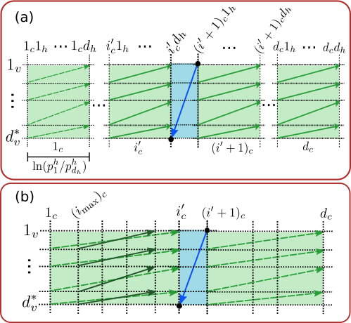
I.1.2 Non-unital transformations

For non-unital transformations, we already found two possible restoring unitaries in Appendix G2 (cf. Eqs. (125) and (126)). If both $V_{1}$ and $V_{2}$ satisfy the required conditions (which means that $p_{1}^{c}>p_{i^{\prime}}^{c}$ and $p_{i^{\prime}+1}^{c}>p_{d_{c}}^{c}$), we can immediately conclude that $V_{1}\oplus V_{2}$ is also a restoring unitary. Note also that since $V_{1}=\oplus_{k=1}^{d_{v}^{\ast}-1}V_{|1_{c}(k+1)_{v}\rangle\leftrightarrow|i^{\prime}_{c}k_{v}\rangle}$ acts on a subspace of $\mathcal{H}_{c}\otimes\mathcal{H}_{v}$, $\mathcal{H}_{n,N}$ is more properly described as $\mathcal{H}_{n,N}=\textrm{span}\{|i_{c}\rangle\}_{i=n}^{N}\otimes\mathcal{H}_{v}$, where $|n_{c}\rangle=|1_{c}\rangle$ and $|N_{c}\rangle=|i^{\prime}_{c}\rangle$. Similarly, $V_{2}=\oplus_{k=1}^{d_{v}^{\ast}-1}V_{|(i^{\prime}+1)_{c}(k+1)_{v}\rangle\leftrightarrow|d_{c}k_{v}\rangle}$ acts on a subspace $\mathcal{H}_{n,N}\subset\mathcal{H}_{c}\otimes\mathcal{H}_{v}$, where $|n_{c}\rangle=|(i^{\prime}+1)_{c}\rangle$ and $|N_{c}\rangle=|d_{c}\rangle$.

Other restoring unitaries can be identified as follows:

1. If $p_{1}^{c}>p_{i^{\prime}}^{c}$, consider the set $\{(n,N)\}_{n,N}=\{(i,i^{\prime}+1-i)\}_{i=1}^{i_{\textrm{max}}}$, where $i_{\textrm{max}}$ is the maximum value of $i$ such that $p_{i}^{c}p_{k+1}^{v}-p_{i^{\prime}+1-i}^{c}p_{k}^{v}>0$ for all $1\leq k\leq d_{v}^{\ast}-1$. In this way, all the partial swaps $\{V_{|i_{c}(k+1)_{v}\rangle\leftrightarrow|(i^{\prime}+1-i)_{c}k_{v}\rangle}\}_{i=1}^{i_{\textrm{max}}}$ generate positive currents $J_{|(k+1)_{v}\rangle\rightarrow|k_{v}\rangle}$, and for $1\leq i\leq i_{\textrm{max}}$ any

   $$V_{i}\equiv\oplus_{k=1}^{d_{v}^{\ast}-1}V_{|i_{c}(k+1)_{v}\rangle\leftrightarrow|(i^{\prime}+1-i)_{c}k_{v}\rangle}$$ (137)

   is a valid restoring unitary. Note that, for $i=1$, the previous expression recovers the restoring unitary $V_{1}$.

2. If $p_{i^{\prime}+1}^{c}>p_{d_{c}}^{c}$, consider the set $\{(n,N)\}_{n,N}=\{(i,d_{c}+i^{\prime}+1-i)\}_{i=i^{\prime}+1}^{i_{\textrm{max}}}$, where $i_{\textrm{max}}$ is the maximum value of $i$ such that $p_{i}^{c}p_{k+1}^{v}-p_{d_{c}+i^{\prime}+1-i}^{c}p_{k}^{v}>0$ for all $1\leq k\leq d_{v}^{\ast}-1$. In this way, all the partial swaps $\{V_{|i_{c}(k+1)_{v}\rangle\leftrightarrow|(d_{c}+i^{\prime}+1-i)_{c}k_{v}\rangle}\}_{i=i^{\prime}+1}^{i_{\textrm{max}}}$ generate positive currents $J_{|(k+1)_{v}\rangle\rightarrow|k_{v}\rangle}$, and for $i^{\prime}+1\leq i\leq i{}_{\textrm{max}}$ any

   $$V_{i}\equiv\oplus_{k=1}^{d_{v}^{\ast}-1}V_{|i_{c}(k+1)_{v}\rangle\leftrightarrow|(d_{c}+i^{\prime}+1-i)_{c}k_{v}\rangle}$$ (138)

   is a valid restoring unitary. Using this notation, $V_{i^{\prime}+1}$ coincides with $V_{2}$.

I.2 Optimal cooling of a qubit using another qubit as hot object

We resort now to results derived in the preceding section to address the problem of maximizing the cooling of a qubit. Specifically, we will consider a transformation $\rho=\rho_{c}\otimes\rho_{h}\otimes\rho_{v}\overset{\textrm{CC}}{\longrightarrow}U\rho U^{\dagger}$, where $\rho_{c}$ and $\rho_{h}$ are both states of two-level systems, and $U=U_{i^{\prime},1,d_{v}^{\ast}-1}\oplus V_{\textrm{res},hv}$. For two-level systems, the index $i^{\prime}$ in the cooling unitary $U_{i^{\prime},1,d_{v}^{\ast}-1}$ only admits the value $i^{\prime}=1$. This yields $U_{1,1,d_{v}^{\ast}-1}=U_{|2_{c}1_{h}1_{v}\rangle\leftrightarrow|1_{c}2_{h}d_{v}^{\ast}\rangle}$, and $V_{\textrm{res},hv}=\oplus_{k=1}^{d_{v}^{\ast}-1}V_{|1_{h}(k+1)_{v}\rangle\leftrightarrow|2_{h}k_{v}\rangle}$.

Since $J_{|(i^{\prime}+1)_{c}\rangle\rightarrow|i^{\prime}_{c}\rangle}=\mathcal{J}_{\textrm{min}}$, maximizing $J_{|(i^{\prime}+1)_{c}\rangle\rightarrow|i^{\prime}_{c}\rangle}$ is tantamount to maximize the loop current $\mathcal{J}_{\textrm{min}}$ (cf. Remark 10). Specifically, we will optimize$\mathcal{J}_{\textrm{min}}$ with respect to the eigenvalues of the state $\rho_{v}$. First, we will show that $\mathcal{J}_{\textrm{min}}$ is maximized by eigenvalues $\{\bar{p}_{k}^{v}\}_{k=1}^{d_{v}^{\ast}}$ such that $\mathcal{U}_{1,1,d_{v}^{\ast}-1}\oplus\left(\oplus_{k=1}^{d_{v}^{\ast}-1}\mathcal{V}_{|1_{h}(k+1)_{v}\rangle\leftrightarrow|2_{h}k_{v}\rangle}\right)$ generates a uniform loop. In other words, a maximum $\mathcal{J}_{\textrm{min}}$ is achieved when all the swap currents in (134) have the same magnitude. For this to happen, the eigenvalues $\{\bar{p}_{k}^{v}\}_{k=1}^{d_{v}^{\ast}}$ must satisfy the set of linear equations

$$\mathcal{J}_{|1_{v}\rangle\rightarrow|d_{v}^{\ast}\rangle}=\mathcal{J}_{|(k+1)_{v}\rangle\rightarrow|k_{v}\rangle},\textrm{ for }1\leq k\leq d_{v}^{\ast}-1.$$ (139)

Explicitly,

$$a\bar{p}_{1}^{v}-b\bar{p}_{d_{v}^{\ast}}^{v}=c\bar{p}_{k+1}^{v}-d\bar{p}_{k}^{v},$$ (140)

for $1\leq k\leq d_{v}^{\ast}-1$, with coefficients

$$\{a,b;c,d\}=\{p_{2}^{c}p_{1}^{h},p_{1}^{c}p_{2}^{h};p_{1}^{h},p_{2}^{h}\}.$$ (141)

In this way, the coefficients $a$ and $b$ reproduce the swap current $\mathcal{J}_{|1_{v}\rangle\rightarrow|d_{v}^{\ast}\rangle}$ (generated by $\mathcal{U}_{1,1,d_{v}^{\ast}-1}$), and the coefficients $c$ and $d$ reproduce the swap current $\mathcal{J}_{|(k+1)_{v}\rangle\rightarrow|k_{v}\rangle}$ (generated by $\mathcal{V}_{|1_{h}(k+1)_{v}\rangle\leftrightarrow|2_{h}k_{v}\rangle}$). After proving that $\{\bar{p}_{k}^{v}\}_{k=1}^{d_{v}^{\ast}}$ are optimal, we will proceed to their evaluation.

I.2.1 Proof of optimality of $\{\bar{p}_{k}^{v}\}_{k=1}^{d_{v}^{\ast}}$

The proof that we will provide in the following is not restricted to the example of optimal cooling considered here. More generally, suppose that the swap currents at the r.h.s. of Eqs. (139) are given by $\mathcal{J}_{|(k+1)_{v}\rangle\rightarrow|k_{v}\rangle}=c_{k+1}\bar{p}_{k+1}^{v}-d_{k}\bar{p}_{k}^{v}$, where $c_{k+1}$ and $d_{k}$ are positive coefficients that may depend on $k$. Suppose also that the only condition on the coefficients $a$ and $b$ in $\mathcal{J}_{|1_{v}\rangle\rightarrow|d_{v}^{\ast}\rangle}=a\bar{p}_{1}^{v}-b\bar{p}_{d_{v}^{\ast}}^{v}$ is that they are also positive. In this way, the generalized form of (139) and (140) reads

$$\mathcal{J}_{|1_{v}\rangle\rightarrow|d_{v}^{\ast}\rangle} =\mathcal{J}_{|(k+1)_{v}\rangle\rightarrow|k_{v}\rangle},$$

$$\Leftrightarrow a\bar{p}_{1}^{v}-b\bar{p}_{d_{v}^{\ast}}^{v} =c_{k+1}\bar{p}_{k+1}^{v}-d_{k}\bar{p}_{k}^{v},$$ (142)

for $1\leq k\leq d_{v}^{\ast}-1$, with Eq. (141) being a particular instance of the general coefficients $\{a,b;c_{k+1},d_{k}\}_{k=1}^{d_{v}^{\ast}-1}$ previously described.

Now, let $\bar{\mathcal{J}}_{\textrm{min}}=\mathcal{J}_{|1_{v}\rangle\rightarrow|d_{v}^{\ast}\rangle}=\mathcal{J}_{|(k+1)_{v}\rangle\rightarrow|k_{v}\rangle}$ denote the loop current resulting from the solution of Eqs. (142). What we shall prove is that the current $\mathcal{J}_{\textrm{min}}$ obtained from any other set of eigenvalues $\{p_{k}^{v}\}_{k=1}^{d_{v}^{\ast}}$ is such that $\mathcal{J}_{\textrm{min}}<\bar{\mathcal{J}}_{\textrm{min}}$. To that end, we write $p_{k}^{v}$ as $p_{k}^{v}=\bar{p}_{k}^{v}+\delta_{k}$, with the variations $\{\delta_{k}\}_{k=1}^{d_{v}^{\ast}}$ constrained in such a way that $\{p_{k}^{v}\}_{k=1}^{d_{v}^{\ast}}$ constitutes a proper probability distribution. This gives rise to the following variations in the swap currents (cf. (142)):

$$\delta\mathcal{J}_{|1_{v}\rangle\rightarrow|d_{v}^{\ast}\rangle} =a\delta_{1}-b\delta_{d_{v}^{\ast}},$$ (143)

$$\delta\mathcal{J}_{|(k+1)_{v}\rangle\rightarrow|k_{v}\rangle} =c_{k+1}\delta_{k+1}-d_{k}\delta_{k}.$$ (144)

If we can show that at least one of these variations must be negative, it follows that the loop current corresponding to $\{p_{k}^{v}\}_{k=1}^{d_{v}^{\ast}}$ satisfies:

$$\mathcal{J}_{\textrm{min}} =\textrm{min}\left\{\mathcal{J}_{|1_{v}\rangle\rightarrow|d_{v}^{\ast}\rangle}+\delta\mathcal{J}_{|1_{v}\rangle\rightarrow|d_{v}^{\ast}\rangle},\right.$$

$$\quad\quad\quad\left.\textrm{min}_{l\leq k\leq l^{\prime}}\left(\mathcal{J}_{|(k+1)_{v}\rangle\rightarrow|k_{v}\rangle}+\delta\mathcal{J}_{|(k+1)_{v}\rangle\rightarrow|k_{v}\rangle}\right)\right\}$$

$$<\bar{\mathcal{J}}_{\textrm{min}},$$ (145)

where $\mathcal{J}_{|1_{v}\rangle\rightarrow|d_{v}^{\ast}\rangle}$ and $\mathcal{J}_{|(k+1)_{v}\rangle\rightarrow|k_{v}\rangle}$ are given in Eqs. (142).

Let us see that this is indeed the case. We start by pointing out two (mutually exclusive) possibilities that the signs of the variations $\{\delta_{k}\}_{k=1}^{d_{v}^{\ast}}$ must adhere to. Either $\{\delta_{k}\leq 0\}_{k=1}^{k^{\prime}-1}$ or $\{\delta_{k}>0\}_{k=1}^{k^{\prime}-1}$, for $k^{\prime}\in\{1,2,...,d_{v}^{\ast}\}$. The first (second) option means that $k^{\prime}-1$ is the maximum $k$ such that $\delta_{k}\leq 0$ ($\delta_{k}>0$), and thus $\delta_{k^{\prime}}>0$ ($\delta_{k^{\prime}}\leq 0$). Note also that $k^{\prime}=d_{v}^{\ast}+1$ is not included, because it is not possible to have $\{\delta_{k}\leq 0\}_{k=1}^{d_{v}^{\ast}}$ or $\{\delta_{k}>0\}_{k=1}^{d_{v}^{\ast}}$ due to the normalization constraint $\sum_{k}p_{k}^{v}=\sum_{k}\bar{p}_{k}^{v}+\sum_{k}\delta_{k}=1+\sum_{k}\delta_{k}=1$. The examination of both options leads to:

1. If $\{\delta_{k}\leq 0\}_{k=1}^{k^{\prime}-1}$, $\delta_{k^{\prime}}>0$ and consequently $\delta\mathcal{J}_{|(k^{\prime}+1)_{v}\rangle\rightarrow|k^{\prime}_{v}\rangle}>0$ only if $\delta_{k^{\prime}+1}>0$ (cf. Eq. (144)). Therefore, $\delta\mathcal{J}_{|(k^{\prime}+2)_{v}\rangle\rightarrow|(k^{\prime}+1)_{v}\rangle}>0$ only if $\delta_{k^{\prime}+2}>0$, and, by recursively applying this argument, $\delta\mathcal{J}_{|d_{v}^{\ast}\rangle\rightarrow|(d_{v}^{\ast}-1)_{v}\rangle}>0$ only if $\delta_{d_{v}^{\ast}}>0$. In this way, we conclude that $\delta_{1}\leq 0$ and $\delta_{d_{v}^{\ast}}>0$. Using Eq. (143), this implies that $\delta\mathcal{J}_{|1_{v}\rangle\rightarrow|d_{v}^{\ast}\rangle}<0$.

2. If $\{\delta_{k}>0\}_{k=1}^{k^{\prime}-1}$, $\delta_{k^{\prime}}\leq 0$ and consequently $\delta\mathcal{J}_{|k^{\prime}_{v}\rangle\rightarrow|(k^{\prime}-1)_{v}\rangle}<0$, according to (144).

This completes the proof of Eq. (145).

I.2.2 Evaluation of $\{\bar{p}_{k}^{v}\}_{k=1}^{d_{v}^{\ast}}$ and corresponding cooling current

The usefulness of the general proof given before will become apparent in the next section and in Appendix L. Now, we return to example of optimal cooling and focus on the solution of Eqs. (140). To that end, we will obtain a sum of the form $\sum_{k=1}^{k^{\prime}}g_{k}\mathcal{J}_{|(k+1)_{v}\rangle\rightarrow|k_{v}\rangle}$, with weights $g_{k}$ chosen in such a way that only terms proportional to $\bar{p}_{k^{\prime}+1}^{v}$ and $\bar{p}_{1}^{v}$ survive. For example, by defining $\zeta\equiv c/d$, we have that:

$$\mathcal{J}_{|2_{v}\rangle\rightarrow|1_{v}\rangle}+\zeta\mathcal{J}_{|3_{v}\rangle\rightarrow|2_{v}\rangle}=c\zeta\bar{p}_{3}^{v}-d\bar{p}_{1}^{v}.$$ (146)

As we will see, this method will lead us to a closed solution for all $\bar{p}_{k^{\prime}}^{v}\in\{\bar{p}_{k}^{v}\}_{k=1}^{d_{v}^{\ast}}$.

Let us prove by induction that weights $g_{k}=\zeta^{k-1}$ yield

$$\sum_{k=1}^{k^{\prime}}\zeta^{k-1}\mathcal{J}_{|(k+1)_{v}\rangle\rightarrow|k_{v}\rangle}=c\zeta^{k^{\prime}-1}\bar{p}_{k^{\prime}+1}^{v}-d\bar{p}_{1}^{v}.$$ (147)

The validity for $k^{\prime}=2$ is manifested in (146). Assuming that Eq. (147) holds for $k^{\prime}$, for $k^{\prime}+1$ it holds that

$$\sum_{k=1}^{k^{\prime}+1}\zeta^{k-1}\mathcal{J}_{|(k+1)_{v}\rangle\rightarrow|k_{v}\rangle} =\sum_{k=1}^{k^{\prime}}\zeta^{k-1}\mathcal{J}_{|(k+1)_{v}\rangle\rightarrow|k_{v}\rangle}$$

$$\quad+\zeta^{k^{\prime}}\mathcal{J}_{|(k^{\prime}+2)_{v}\rangle\rightarrow|(k^{\prime}+1)_{v}\rangle}$$

$$=c\zeta^{k^{\prime}-1}\bar{p}_{k^{\prime}+1}^{v}-d\bar{p}_{1}^{v}$$

$$\quad+\zeta^{k^{\prime}}\left(c\bar{p}_{k^{\prime}+2}^{v}-d\bar{p}_{k^{\prime}+1}^{v}\right)$$

$$=c\zeta^{k^{\prime}}\bar{p}_{k^{\prime}+2}^{v}-d\bar{p}_{1}^{v},$$ (148)

where $\mathcal{J}_{|(k^{\prime}+2)_{v}\rangle\rightarrow|(k^{\prime}+1)_{v}\rangle}$ is written as $c\bar{p}_{k^{\prime}+2}^{v}-d\bar{p}_{k^{\prime}+1}^{v}$ (cf. (140)) in the second equality. This shows that Eq. (147) is also valid for any $k^{\prime}\geq 2$. For $k^{\prime}=1$ it is straightforward to check that the correct form of $\mathcal{J}_{|2_{v}\rangle\rightarrow|1_{v}\rangle}$ is also recovered.

By isolating $\bar{p}_{k^{\prime}+1}^{v}$ from (147) we obtain:

$$\bar{p}_{k^{\prime}+1}^{v} =\frac{\zeta^{1-k^{\prime}}}{c}\left[d\bar{p}_{1}^{v}+\sum_{k=1}^{k^{\prime}}\zeta^{k-1}\mathcal{J}_{|(k+1)_{v}\rangle\rightarrow|k_{v}\rangle}\right]$$

$$=\frac{\zeta^{1-k^{\prime}}}{c}\left[d\bar{p}_{1}^{v}+\left(\sum_{k=1}^{k^{\prime}}\zeta^{k-1}\right)\mathcal{J}_{|1_{v}\rangle\rightarrow|d_{v}^{\ast}\rangle}\right]$$

$$=\frac{\zeta^{1-k^{\prime}}}{c}\left[d\bar{p}_{1}^{v}+\frac{1-\zeta^{k^{\prime}}}{1-\zeta}(a\bar{p}_{1}^{v}-b\bar{p}_{d_{v}^{\ast}}^{v})\right],$$ (149)

where Eq. (139) is applied in the second line and in the third line we evaluate the geometric series $\sum_{k=1}^{k^{\prime}}\zeta^{k-1}$. The expression for $\bar{p}_{d_{v}^{\ast}}^{v}$ can be readily obtained by setting $k^{\prime}=d_{v}^{\ast}-1$ in (149), and performing a few algebraic manipulations:

$$\bar{p}_{d_{v}^{\ast}}^{v} =\left(d+a\frac{1-\zeta^{d_{v}^{\ast}-1}}{1-\zeta}\right)\frac{\bar{p}_{1}^{v}}{c\zeta^{d_{v}^{\ast}-2}+b\frac{1-\zeta^{d_{v}^{\ast}-1}}{1-\zeta}}$$

$$=\frac{\left(d(\zeta-1)+a(\zeta^{d_{v}^{\ast}-1}-1)\right)\bar{p}_{1}^{v}}{c\zeta^{d_{v}^{\ast}-2}(\zeta-1)+b(\zeta^{d_{v}^{\ast}-1}-1)}.$$ (150)

If $\bar{p}_{d_{v}^{\ast}}^{v}$ in (150) is inserted back into (149), we obtain all the eigenvalues $\{\bar{p}_{k}^{v}\}_{k=2}^{d_{v}^{\ast}}$ in terms of $\bar{p}_{1}^{v}$ and the coefficients $\{a,b;c,d\}$. Finally, the eigenvalue $\bar{p}_{1}^{v}$ can be deduced via probability conservation $\bar{p}_{1}^{v}+\sum_{k^{\prime}=1}^{d_{v}^{\ast}-1}\bar{p}_{k^{\prime}+1}^{v}=1$.

As implied by Remark 10, the cooling currrent $\mathcal{J}_{|(i^{\prime}+1)_{c}\rangle\rightarrow|i^{\prime}_{c}\rangle}$ can be obtained from $\mathcal{J}_{|(i^{\prime}+1)_{c}\rangle\rightarrow|i^{\prime}_{c}\rangle}=\mathcal{J}_{|1_{v}\rangle\rightarrow|d_{v}^{\ast}\rangle}$, and thus $\mathcal{J}_{|(i^{\prime}+1)_{c}\rangle\rightarrow|i^{\prime}_{c}\rangle}=a\bar{p}_{1}^{v}-b\bar{p}_{d_{v}^{\ast}}^{v}$ (cf. (139) and (140)). After setting $a=p_{2}^{c}p_{1}^{h}$ and $b=p_{1}^{c}p_{2}^{h}$ and substituting $\bar{p}_{d_{v}^{\ast}}^{v}$ as given in (150), we find:

$$\mathcal{J}_{|(i^{\prime}+1)_{c}\rangle\rightarrow|i^{\prime}_{c}\rangle} =\frac{ac\zeta^{d_{v}^{\ast}-2}(\zeta-1)-bd(\zeta-1)}{c\zeta^{d_{v}^{\ast}-2}(\zeta-1)+b(\zeta^{d_{v}^{\ast}-1}-1)}\bar{p}_{1}^{v}$$

$$=\frac{(\zeta-1)\left(p_{2}^{c}p_{1}^{h}p_{1}^{h}\zeta^{d_{v}^{\ast}-2}-p_{1}^{c}p_{2}^{h}p_{2}^{h}\right)}{p_{1}^{h}\zeta^{d_{v}^{\ast}-2}(\zeta-1)+p_{1}^{c}p_{2}^{h}(\zeta^{d_{v}^{\ast}-1}-1)}\bar{p}_{1}^{v}$$

$$=\frac{(\zeta-1)p_{2}^{h}\left(p_{2}^{c}\zeta^{d_{v}^{\ast}}-p_{1}^{c}\right)}{\zeta^{d_{v}^{\ast}-1}(\zeta-1)+p_{1}^{c}(\zeta^{d_{v}^{\ast}-1}-1)}\bar{p}_{1}^{v}.$$ (151)

Since this is the maximum value of the cooling current, as per Remark 10, we express it as $J_{\textrm{cool}}^{\textrm{max}}$ in the main text.

I.3 Maximization of the loop current for more general catalytic unitaries

We conclude this appendix by illustrating a first scenario where the optimality proof concerning Eqs. (142) is useful. Although here we will obtain currents with coefficients $c_{k+1}$ and $d_{k}$ that do not depend on $k$ (i.e. $c_{k+1}=c$ and $d_{k}=d$), the resulting set $\{a,b;c,d\}$ characterizes swap currents $\{\mathcal{J}_{|1_{v}\rangle\rightarrow|d_{v}^{\ast}\rangle},\{\mathcal{J}_{|(k+1)_{v}\rangle\rightarrow|k_{v}\rangle}\}_{k=1}^{d_{v}^{\ast}-1}$ related to evolutions much more general than the unitary $\mathcal{U}_{1,1,d_{v}^{\ast}-1}\oplus\left(\oplus_{k=1}^{d_{v}^{\ast}-1}\mathcal{V}_{|1_{h}(k+1)_{v}\rangle\leftrightarrow|2_{h}k_{v}\rangle}\right)$ considered in Appendix I2. For these evolutions, the proof given in I2 implies that the corresponding loop current is maximized by eigenvalues $\{\bar{p}_{k}^{v}\}$ that solve Eqs. (142). While the motivation for this maximization may not always be evident, it is of particular interest for catalytic and cooling transformations, as highlighted in Remark 10.

In what follows we consider catalytic unitaries where the restoring unitary satisfies Eq. (131) and the generalization indicated by Remark 9 also takes place. By setting $l=1$ and $l^{\prime}=d_{v}^{\ast}-1$, we thus consider unitaries $U_{d_{v}^{\ast}}\oplus\left(\oplus_{k=1}^{d_{v}^{\ast}-1}V_{k}\right)$, where $U_{d_{v}^{\ast}}=\oplus_{\psi,\varphi\textrm{ free}}U_{|\psi\rangle\leftrightarrow|\varphi\rangle}$ acts on $\mathcal{H}_{c}\otimes\mathcal{H}_{h}\otimes\textrm{span}\{|1_{v}\rangle,|d_{v}^{\ast}\rangle\}$ and $V_{k}=\oplus_{n,N}V_{|n_{ch}(k+1)_{v}\rangle\leftrightarrow|N_{ch}k_{v}\rangle}$.

Proposition 4. Let $U_{d_{v}^{\ast}}\oplus\left(\oplus_{k=1}^{d_{v}^{\ast}-1}V_{k}\right)$ be a unitary applied on ${\normalcolor\rho_{ch}\otimes\rho_{v}^{\ast}}$, where $\rho_{ch}$ is a generic state of the compound $ch$ and $\rho_{v}^{\ast}=\sum_{k=1}^{d_{v}^{\ast}-1}p_{k}^{v}|k_{v}\rangle\langle k_{v}|$ is a full-rank catalyst state. Under the assumption that $U_{d_{v}^{\ast}}\oplus\left(\oplus_{k=1}^{d_{v}^{\ast}-1}V_{k}\right)$ generates a loop $\{J_{|1_{v}\rangle\rightarrow|d_{v}^{\ast}\rangle}\}\cup\{J_{|(k+1)_{v}\rangle\rightarrow|k_{v}\rangle}\}_{k=1}^{d_{v}^{\ast}-1}$, the loop current $\mathcal{J}_{\textrm{min}}=\textrm{min}\{\mathcal{J}_{|1_{v}\rangle\rightarrow|d_{v}^{\ast}\rangle},\mathcal{J}_{|(k+1)_{v}\rangle\rightarrow|k_{v}\rangle}\}_{k=1}^{d_{v}^{\ast}-1}$ is maximized by catalyst eigenvalues $\{\bar{p}_{k}^{v}\}_{k=1}^{d_{v}^{\ast}-1}$ that satisfy Eqs. (142). Accordingly, the optimal unitary is a permutation that we denote as $\mathcal{U}_{d_{v}^{\ast}}\oplus\left(\oplus_{k=1}^{d_{v}^{\ast}-1}\mathcal{V}_{k}\right)$, with

$$\mathcal{U}_{d_{v}^{\ast}} =\oplus_{\psi,\varphi\textrm{ free}}\mathcal{U}_{|\varphi_{ch}1_{v}\rangle\leftrightarrow|\psi_{ch}d_{v}^{\ast}\rangle},$$ (152)

$$\mathcal{V}_{k} =\oplus_{n,N}\mathcal{V}_{|n_{ch}(k+1)_{v}\rangle\leftrightarrow|N_{ch}k_{v}\rangle},$$ (153)

for $k\in\{1,2,...,d_{v}^{\ast}-1\}$.

Proof. Taking into account the proof given in Appendix I2, we only need to express $\mathcal{J}_{|1_{v}\rangle\rightarrow|d_{v}^{\ast}\rangle}$ and $\mathcal{J}_{|(k+1)_{v}\rangle\rightarrow|k_{v}\rangle}$ as in Eqs. (142). Specifically, we have that, if Eqs. (152) and (153) hold,

$$\mathcal{J}_{|1_{v}\rangle\rightarrow|d_{v}^{\ast}\rangle} =\sum_{\psi,\varphi\textrm{ free}}\mathcal{J}_{|\varphi_{ch}1_{v}\rangle\rightarrow|\psi_{ch}d_{v}^{\ast}\rangle}$$

$$=\sum_{\psi,\varphi\textrm{ free}}\left(p_{\varphi}^{ch}\bar{p}_{1}^{v}-p_{\psi}^{ch}\bar{p}_{d_{v}^{\ast}}^{v}\right)$$

$$=\left(\sum_{\varphi\textrm{ free}}p_{\varphi}^{ch}\right)\bar{p}_{1}^{v}-\left(\sum_{\psi\textrm{ free}}p_{\psi}^{ch}\right)\bar{p}_{d_{v}^{\ast}}^{v}$$

$$\equiv a\bar{p}_{1}^{v}-b\bar{p}_{d_{v}^{\ast}}^{v},$$ (154)

where the first line obeys (90), and

$$\mathcal{J}_{|(k+1)_{v}\rangle\rightarrow|k_{v}\rangle} =\sum_{n,N}\mathcal{J}_{|n_{ch}(k+1)_{v}\rangle\rightarrow|N_{ch}k_{v}\rangle}$$

$$=\sum_{n,N}\left(p_{n}^{ch}\bar{p}_{k+1}^{v}-p_{N}^{ch}\bar{p}_{k}^{v}\right)$$

$$=\left(\sum_{n}p_{n}^{ch}\right)\bar{p}_{k+1}^{v}-\left(\sum_{N}p_{N}^{ch}\right)\bar{p}_{k}^{v}$$

$$\equiv c\bar{p}_{k+1}^{v}-d\bar{p}_{k}^{v},$$ (155)

where the first line obeys (133).

Note that in this case the coefficients $c$ and $d$ are independent of $k$ (i.e. $c_{k+1}=c$ and $d_{k}=d$). Furthermore, note also that Eqs. (152) and (153) recover the unitary for optimal cooling $\mathcal{U}_{1,1,d_{v}^{\ast}-1}\oplus\left(\oplus_{k=1}^{d_{v}^{\ast}-1}\mathcal{V}_{|1_{h}(k+1)_{v}\rangle\leftrightarrow|2_{h}k_{v}\rangle}\right)$, by setting $\mathcal{U}_{d_{v}^{\ast}}=\mathcal{U}_{|2_{c}1_{h}1_{v}\rangle\leftrightarrow|1_{c}d_{h}d_{v}^{\ast}\rangle}$ and $\mathcal{V}_{k}=\mathcal{V}_{|1_{h}(k+1)_{v}\rangle\leftrightarrow|2_{h}k_{v}\rangle}$.

Remark 11. Since the coefficients $c$ and $d$ in (154) and (155) are independent of $k$, the optimal eigenvalues $\{\bar{p}_{k}^{v}\}_{k}$ are provided by Eqs. (149) and (150). Moreover, if $\mathcal{J}_{|1_{v}\rangle\rightarrow|d_{v}^{\ast}\rangle}=\mathcal{J}_{|(i^{\prime}+1)_{c}\rangle\rightarrow|i^{\prime}_{c}\rangle}$ (which occurs e.g. if $\mathcal{U}_{d_{v}^{\ast}}=\mathcal{U}_{|i^{\prime}_{c}d_{h}d_{v}^{\ast}\rangle\leftrightarrow|(i^{\prime}+1)_{c}1_{h}1_{v}\rangle}$), the resulting current $\mathcal{J}_{\textrm{min}}$ satisfies the first line of (151).

Appendix J PROOF OF THEOREM 3 AND EXAMPLE OF CATALYTIC COOLING ENHANCEMENT

To prove Theorem 3 we shall employ the following lemma, which provides an optimal unitary to cool the cold qubit using only the hot object. This unitary maximizes the ground population of the cold qubit, keeping in mind that reducing the energy of a two-level system is equivalent to increase its ground population. In addition, we stress that in this setting the state $\rho_{c}\otimes\rho_{h}$ is non-passive with respect to $H_{c}$.

Lemma 4 (maximum cooling of a qubit using only the hot object). If $\rho_{c}=\sum_{i=1}^{2}p_{i}^{c}|i_{c}\rangle\langle i_{c}|$ is a general state of a qubit and $\rho_{h}=\sum_{j=1}^{d_{h}}p_{j}^{h}|j_{h}\rangle\langle j_{h}|$ is a general state of a hot object, the ground population of the cold qubit is maximized by a permutation

$$\tilde{\mathcal{U}}\equiv\oplus_{j=1}^{j_{\textrm{max}}}\mathcal{U}{}_{|1_{c}(d_{h}-j_{\textrm{max}}+j)_{h}\rangle\leftrightarrow|2_{c}(j_{\textrm{max}}-j+1)_{h}\rangle},$$ (156)

where $j_{\textrm{max}}$ is the maximum value of $j$ such that $p_{2}^{c}p_{j}^{h}>p_{1}^{c}p_{d_{h}-j+1}^{h}$.

Proof. We define the sets of indices $A=\{j\}_{1\leq j\leq j_{\textrm{max}}}$, $A^{\prime}=\{j\}_{j_{\textrm{max}}+1\leq j\leq d_{h}}$, $B=\{j\}_{d_{h}-j_{\textrm{max}}+1\leq j\leq d_{h}}$, and $B^{\prime}=\{j\}_{1\leq j\leq d_{h}-j_{\textrm{max}}}$. From these definitions, we note immediately that $A^{\prime}$ is the complement of $A$, and $B^{\prime}$ is the complement of $B$. Accordingly, the state $\rho_{c}\otimes\rho_{h}$ can be expressed as

$$\rho_{c}\otimes\rho_{h} =\sum_{j\in B}p_{1}^{c}p_{j}^{h}|1_{c}j_{h}\rangle\langle 1_{c}j_{h}|+\sum_{j\in B^{\prime}}p_{1}^{c}p_{j}^{h}|1_{c}j_{h}\rangle\langle 1_{c}j_{h}|$$

$$\quad+\sum_{j\in A}p_{2}^{c}p_{j}^{h}|2_{c}j_{h}\rangle\langle 2_{c}j_{h}|+\sum_{j\in A^{\prime}}p_{2}^{c}p_{j}^{h}|2_{c}j_{h}\rangle\langle 2_{c}j_{h}|.$$ (157)

According to (156), the effect of $\tilde{\mathcal{U}}$ is to swap the eigenstates in the set $\{|1_{c}j_{h}\rangle\}_{j\in B}$ with the eigenstates in the set $\{|2_{c}j_{h}\rangle\}_{j\in A}$. For example, $|1_{c}(d_{h}-j_{\textrm{max}}+1)_{h}\rangle$ is swapped with $|2_{c}(j_{\textrm{max}})_{h}\rangle$, $|1_{c}(d_{h}-j_{\textrm{max}}+2)_{h}\rangle$ is swapped with $|2_{c}(j_{\textrm{max}}-1)_{h}\rangle$, and so forth, up to $|1_{c}d_{h}\rangle$ is swapped with $|2_{c}1_{h}\rangle$. Since this is equivalent to exchange the eigenvalues corresponding to $\{|1_{c}j_{h}\rangle\}_{j\in B}$ with those corresponding to $\{|2_{c}j_{h}\rangle\}_{j\in A}$, the transformed state $\tilde{\mathcal{U}}(\rho_{c}\otimes\rho_{h})\tilde{\mathcal{U}}^{\dagger}$ reads

$$\tilde{\mathcal{U}}(\rho_{c}\otimes\rho_{h})\tilde{\mathcal{U}}^{\dagger} =\sum_{j\in A}p_{2}^{c}p_{j}^{h}|1_{c}j_{h}\rangle\langle 1_{c}j_{h}|+\sum_{j\in B^{\prime}}p_{1}^{c}p_{j}^{h}|1_{c}j_{h}\rangle\langle 1_{c}j_{h}|$$

$$\quad+\sum_{j\in B}p_{1}^{c}p_{j}^{h}|2_{c}j_{h}\rangle\langle 2_{c}j_{h}|+\sum_{j\in A^{\prime}}p_{2}^{c}p_{j}^{h}|2_{c}j_{h}\rangle\langle 2_{c}j_{h}|.$$ (158)

Let us see now that $\tilde{\mathcal{U}}(\rho_{c}\otimes\rho_{h})\tilde{\mathcal{U}}^{\dagger}$ is passive with respect to $|2_{c}\rangle\langle 2_{c}|$, which amounts to the impossibility to further reduce $\bigl{\langle}|2_{c}\rangle\langle 2_{c}|\bigr{\rangle}$ via unitary evolutions (i.e. $\Delta\bigl{\langle}|2_{c}\rangle\langle 2_{c}|\bigr{\rangle}\geq 0$ if $\tilde{\mathcal{U}}(\rho_{c}\otimes\rho_{h})\tilde{\mathcal{U}}^{\dagger}$ is evolved unitarily). Since $\Delta\bigl{\langle}|2_{c}\rangle\langle 2_{c}|\bigr{\rangle}=-\Delta\bigl{\langle}|1_{c}\rangle\langle 1_{c}|\bigr{\rangle}$ (by probability conservation), this also means that $\Delta\bigl{\langle}|1_{c}\rangle\langle 1_{c}|\bigr{\rangle}\leq 0$ for any unitary applied on $\tilde{\mathcal{U}}(\rho_{c}\otimes\rho_{h})\tilde{\mathcal{U}}^{\dagger}$, and consequenly this state maximizes the ground population $\bigl{\langle}|1_{c}\rangle\langle 1_{c}|\bigr{\rangle}.$

By definition of $j_{\textrm{max}}$, $p_{2}^{c}p_{j_{\textrm{max}}}^{h}>p_{1}^{c}p_{d_{h}-j_{\textrm{max}}+1}^{h}$. Taking into account the ordering $p_{j}^{h}\geq p_{j+1}^{h}$, and the definitions of $A$ and $B$, the inequality $p_{2}^{c}p_{j_{\textrm{max}}}^{h}>p_{1}^{c}p_{d_{h}-j_{\textrm{max}}+1}^{h}$ can be rewritten as

$$\textrm{min}_{j\in A}p_{2}^{c}p_{j}^{h}>\textrm{max}_{j\in B}p_{1}^{c}p_{j}^{h}.$$ (159)

Similarly, since $j=j_{\textrm{max}}$ is the maximum value such that $p_{2}^{c}p_{j}^{h}>p_{1}^{c}p_{d_{h}-j+1}^{h}$, we also have that $p_{2}^{c}p_{j_{\textrm{max}}+1}^{h}\leq p_{1}^{c}p_{d_{h}-j_{\textrm{max}}}^{h}$, which is equivalent to

$$\textrm{min}_{j\in B^{\prime}}p_{1}^{c}p_{j}^{h}\geq\textrm{max}_{j\in A^{\prime}}p_{2}^{c}p_{j}^{h}.$$ (160)

Finally, the ordering $p_{j}^{h}\geq p_{j+1}^{h}$ and the definitions of the sets $A$, $A^{\prime}$, $B$, and $B^{\prime}$, lead to:

$$\textrm{min}_{j\in A}p_{2}^{c}p_{j}^{h} \geq\textrm{max}_{j\in A^{\prime}}p_{2}^{c}p_{j}^{h},$$ (161)

$$\textrm{min}_{j\in B^{\prime}}p_{1}^{c}p_{j}^{h} \geq\textrm{max}_{j\in B}p_{1}^{c}p_{j}^{h}.$$ (162)

Equations (159)-(162) tell us that the smallest eigenvalue in the first line of (158) must be larger or equal than the largest eigenvalue in the second line. Since $|2_{c}\rangle\langle 2_{c}|=|2_{c}\rangle\langle 2_{c}|\otimes\mathbb{I}_{h}$ has eigenvalue 0 for the eigenstates $\{|1_{c}j_{h}\rangle\}_{j}$, and eigenvalue 1 for the eigenstates $\{|2_{c}j_{h}\rangle\}_{j}$ we conclude that $\tilde{\mathcal{U}}(\rho_{c}\otimes\rho_{h})\tilde{\mathcal{U}}^{\dagger}$ is passive with respect to $|2_{c}\rangle\langle 2_{c}|$.

J.1 Proof of Theorem 3

In the following we shall assume that the eigenvalues of the catalyst satisfy Eq. (115). That is, $\frac{p_{k}}{p_{k+1}}=\mu>1$, for $1\leq k\leq d_{v}^{\ast}-1$. Moreover, the initial total state is $\rho=\rho_{c}\otimes\rho_{h}\otimes\rho_{v}$.

Given the effect of $\tilde{\mathcal{U}}$, previously described, $\tilde{\mathcal{U}}\otimes\mathbb{I}_{v}$ acts on the subspace

$$\tilde{\mathcal{H}}=\textrm{span}\left(\{|2_{c}j_{h}\rangle\}_{j\in A}\cup\{|1_{c}j_{h}\rangle\}_{j\in B}\right)\otimes\mathcal{H}_{v}.$$ (163)

Now we want to show that, if the conditions of Theorem 3 hold, we can construct a catalytic and cooling unitary $U:\tilde{\mathcal{H}^{\prime}}\rightarrow\tilde{\mathcal{H}^{\prime}}$, where

$$\tilde{\mathcal{H}^{\prime}}=\textrm{span}\left(\{|2_{c}j_{h}\rangle\}_{j\in A^{\prime}}\cup\{|1_{c}j_{h}\rangle\}_{j\in B^{\prime}}\right)\otimes\mathcal{H}_{v}.$$ (164)

Taking into account that $\tilde{\mathcal{H}}$ and $\tilde{\mathcal{H}^{\prime}}$ are orthogonal, the direct sum $\tilde{\mathcal{U}}\oplus U$ yields the total variation (cf. Eqs. (78) and (79)) $\Delta\left\langle H_{c}\right\rangle=\textrm{Tr}\left[H_{c}\left(\tilde{\mathcal{U}}\oplus U\rho\tilde{\mathcal{U}}^{\dagger}\oplus U^{\dagger}-\rho\right)\right]$:

$$\Delta\left\langle H_{c}\right\rangle=\Delta_{\tilde{\mathcal{U}}}\left\langle H_{c}\right\rangle+\Delta_{U}\left\langle H_{c}\right\rangle<\Delta_{\tilde{\mathcal{U}}}\left\langle H_{c}\right\rangle,$$ (165)

where $\Delta_{\tilde{\mathcal{U}}}\left\langle H_{c}\right\rangle=\textrm{Tr}\left[H_{c}\left(\tilde{\mathcal{U}}\rho_{c}\otimes\rho_{h}\tilde{\mathcal{U}}^{\dagger}-\rho_{c}\otimes\rho_{h}\right)\right]$ and $\Delta_{U}\left\langle H_{c}\right\rangle=\textrm{Tr}\left[H_{c}\left(U\rho U^{\dagger}-\rho\right)\right]$.

As a preliminary result that will be used later, let us check that

$$j_{\textrm{max}}\leq d_{h}/2.$$ (166)

If $j_{\textrm{max}}\geq d_{h}/2+1$, we have that $d_{h}-j_{\textrm{max}}+1\leq d_{h}/2<j_{\textrm{max}}$ and consequently $p_{j_{\textrm{max}}}^{h}\leq p_{d_{h}-j_{\textrm{max}}+1}^{h}$. This implies that $p_{2}^{c}p_{j_{\textrm{max}}}^{h}\leq p_{1}^{c}p_{d_{h}-j_{\textrm{max}}+1}^{h}$, in contradiction with the definition of $j_{\textrm{max}}$.

J.1.1 Proof for the case $p_{1}^{h}>p_{d_{h}/2}^{h}$

Let us first provide the conditions for a cooling unitary $U_{\textrm{cool}}:\tilde{\mathcal{H}^{\prime}}\rightarrow\tilde{\mathcal{H}^{\prime}}$. Since $\mu>1$, for sufficiently large $d_{v}$ we have that

$$\mu^{d_{v}-1}=\frac{p_{1}^{v}}{p_{d_{v}}^{v}}>\frac{p_{1}^{c}p_{d_{h}-j_{\textrm{max}}}^{h}}{p_{2}^{c}p_{j_{\textrm{max}}+1}^{h}}.$$ (167)

In this way, the unitary $U_{\textrm{cool}}=U_{|2_{c}(j_{\textrm{max}}+1)_{h}1_{v}\rangle\leftrightarrow|1_{c}(d_{h}-j_{\textrm{max}})_{h}d_{v}\rangle}$ generates a cooling current $J_{|2_{c}\rangle\rightarrow|1_{c}\rangle}$, and a local current $J_{|1_{v}\rangle\rightarrow|d_{v}\rangle}=J_{|2_{c}\rangle\rightarrow|1_{c}\rangle}$. Moreover, both $|2_{c}(j_{\textrm{max}}+1)_{h}\rangle$ and $|1_{c}(d_{h}-j_{\textrm{max}})_{h}\rangle$ belong to $\textrm{span}\left(\{|2_{c}j_{h}\rangle\}_{j\in A^{\prime}}\cup\{|1_{c}j_{h}\rangle\}_{j\in B^{\prime}}\right)$, which guarantees that $U_{\textrm{cool}}$ acts on $\tilde{\mathcal{H}^{\prime}}$.

Our next step is to obtain a chain $\mathbf{ch}_{|d_{v}\rangle\rightarrow|1_{v}\rangle}$ using a proper restoring unitary. From (166) and the ordering $p_{j}^{h}\geq p_{j+1}^{h}$ we have that $p_{d_{h}/2}^{h}\geq p_{d_{h}-j_{\textrm{max}}}^{h}$. Hence, $p_{1}^{h}>p_{d_{h}-j_{\textrm{max}}}^{h}$. If $\mu>1$ is sufficiently small, we can use the inequality $p_{1}^{h}>p_{d_{h}-j_{\textrm{max}}}^{h}$ to enforce the condition

$$\frac{p_{1}^{c}p_{1}^{h}}{p_{1}^{c}p_{d_{h}-j_{\textrm{max}}}^{h}}>\frac{p_{k}^{v}}{p_{k+1}^{v}}=\mu.$$ (168)

This implies that the partial swaps in the direct sum

$$V_{B^{\prime}} =\oplus_{k=1}^{d_{v}-1}V_{|1_{c}1_{h}(k+1)_{v}\rangle\leftrightarrow|1_{c}(d_{h}-j_{\textrm{max}})_{h}k_{v}\rangle}$$

$$=|1_{c}\rangle\langle 1_{c}|\otimes\left(\oplus_{k=1}^{d_{v}-1}V_{|1_{h}(k+1)_{v}\rangle\leftrightarrow|(d_{h}-j_{\textrm{max}})_{h}k_{v}\rangle}\right)$$ (169)

generates the desired chain $\mathbf{ch}_{|d_{v}\rangle\rightarrow|1_{v}\rangle}=\{J_{|(k+1)_{v}\rangle\rightarrow|k_{v}\rangle}\}_{k=1}^{d_{v}-1}$. In addition, all the eigenstates “connected” by these partial swaps belong to $\textrm{span}\{|1_{c}j_{h}\rangle\}_{j\in B^{\prime}}\otimes\mathcal{H}_{v}$, and therefore $V_{B^{\prime}}$ also acts on $\tilde{\mathcal{H}^{\prime}}$ (cf. Remark 2).

Noting that the eigenstates connected in Eq. (169) are orthogonal to those connected by $U_{\textrm{cool}}$, $U_{\textrm{cool}}$ and $V_{B^{\prime}}$ act on orthogonal subspaces of $\tilde{\mathcal{H}^{\prime}}$. Hence, we can construct a direct sum $U=U_{\textrm{cool}}\oplus V_{B^{\prime}}$, with a corresponding loop $\mathbf{ch}_{|d_{v}\rangle\rightarrow|1_{v}\rangle}\cup\{J_{|1_{v}\rangle\rightarrow|d_{v}\rangle}\}$. This loop can be made uniform through a tuning of swap intensities analogous to that used in the sufficiency proof of Theorem 1. That is, by choosing intensities such that $J_{|1_{v}\rangle\rightarrow|d_{v}\rangle}=J_{|(k+1)_{v}\rangle\rightarrow|k_{v}\rangle}=\mathcal{J}_{\textrm{min}}$, where $\mathcal{J}_{\textrm{min}}$ is the minimum swap current in the set $\{\mathcal{J}_{|1_{v}\rangle\rightarrow|d_{v}\rangle},\mathcal{J}_{|(k+1)_{v}\rangle\rightarrow|k_{v}\rangle}\}_{k}$. This guarantees that the transformation $\rho\rightarrow U\rho U^{\dagger}$ is catalytic, as per Remark 7.

Since $V_{B^{\prime}}$ is a controlled unitary where the cold object is the control, it does not change the average energy of the cold object. Therefore, $\Delta_{U}\left\langle H_{c}\right\rangle=\Delta_{\textrm{cool}}\left\langle H_{c}\right\rangle+\Delta_{V_{B^{\prime}}}\left\langle H_{c}\right\rangle=\Delta_{\textrm{cool}}\left\langle H_{c}\right\rangle$. In this way, $\Delta_{U}\left\langle H_{c}\right\rangle$ in Eq. (165) explicitly reads $\Delta_{U}\left\langle H_{c}\right\rangle=J_{|2_{c}\rangle\rightarrow|1_{c}\rangle}(\varepsilon_{1}^{c}-\varepsilon_{2}^{c})<0$.

J.1.2 Proof for the case $p_{d_{h}/2+1}^{h}>p_{d_{h}}^{h}$

The proof is very similar to the previous one, with the only relevant difference being related to the construction of the restoring unitary. From Eq. (166), it follows that $j_{\textrm{max}}+1\leq d_{h}/2+1$ and therefore $p_{2}^{c}p_{j_{\textrm{max}}+1}^{h}\geq p_{2}^{c}p_{d_{h}/2+1}^{h}$. In combination with the hypothesis $p_{d_{h}/2+1}^{h}>p_{d_{h}}^{h}$, we obtain the inequality $p_{2}^{c}p_{j_{\textrm{max}}+1}^{h}>p_{d_{h}}^{h}$, which can be applied to enforce the condition (for $\mu$ sufficiently small):

$$\frac{p_{2}^{c}p_{j_{\textrm{max}}+1}^{h}}{p_{2}^{c}p_{d_{h}}^{h}}>\frac{p_{k}^{v}}{p_{k+1}^{v}}=\mu.$$ (170)

Therefore, the partial swaps in the direct sum

$$V_{A^{\prime}} =\oplus_{k=1}^{d_{v}-1}V_{|2_{c}(j_{\textrm{max}}+1)_{h}(k+1)_{v}\rangle\leftrightarrow|2_{c}d_{h}k_{v}\rangle}$$

$$=|2_{c}\rangle\langle 2_{c}|\otimes\left(\oplus_{k=1}^{d_{v}-1}V_{|(j_{\textrm{max}}+1)_{h}(k+1)_{v}\rangle\leftrightarrow|d_{h}k_{v}\rangle}\right)$$ (171)

generate a chain $\mathbf{ch}_{|d_{v}\rangle\rightarrow|1_{v}\rangle}$. Since these partial swaps connect eigenstates in $\textrm{span}\{|2_{c}j_{h}\rangle\}_{j\in A^{\prime}}\otimes\mathcal{H}_{v}$, $V_{A^{\prime}}$ acts on $\tilde{\mathcal{H}^{\prime}}$.

By choosing $d_{v}$ large enough, Eq. (167) provides the same cooling unitary of the previous case, i.e. $U_{\textrm{cool}}=U_{|2_{c}(j_{\textrm{max}}+1)_{h}1_{v}\rangle\leftrightarrow|1_{c}(d_{h}-j_{\textrm{max}})_{h}d_{v}\rangle}$. Once again, it can be readily checked that $U_{\textrm{cool}}$ and $V_{A^{\prime}}$ act on orthogonal subspaces of $\tilde{\mathcal{H}^{\prime}}$. Given that $V_{A^{\prime}}$ does not change the average energy of the cold qubit, $U=U_{\textrm{cool}}\oplus V_{A^{\prime}}$ also gives rise to a catalytic and cooling transformation that increases the cooling generated by $\tilde{\mathcal{U}}$ (cf. (165)) in the amount $\Delta_{U}\left\langle H_{c}\right\rangle=\Delta_{\textrm{cool}}\left\langle H_{c}\right\rangle<0$.

J.2 Example of catalytic cooling enhancement with $d_{h}$ odd

As explained in the main text, the optimal cooling of a qubit using a three-level hot object leads to a passive state

$$\sigma_{ch} =|1_{c}\rangle\langle 1_{c}|\otimes\left(\sum_{j=1}^{2}p_{1}^{c}p_{j}^{h}|j_{h}\rangle\langle j_{h}|+p_{2}^{c}p_{1}^{h}|3_{h}\rangle\langle 3_{h}|\right)$$

$$\quad+|2_{c}\rangle\langle 2_{c}|\otimes\left(p_{1}^{c}p_{3}^{h}|1_{h}\rangle\langle 1_{h}|+\sum_{j=2}^{3}p_{2}^{c}p_{j}^{h}|j_{h}\rangle\langle j_{h}|\right),$$ (172)

where $\{p_{i}^{c}\}_{i=1}^{2}$ and $\{p_{j}^{h}\}_{j=1}^{3}$ are respectively the eigenvalues of the initial states $\rho_{c}$ and $\rho_{h}$. Hence, we can focus on the additional cooling provided by a proper catalytic transformation $\sigma_{ch}\otimes\rho_{v}\overset{\textrm{CC}}{\longrightarrow}U\sigma_{ch}\otimes\rho_{v}U^{\dagger}$. Since we consider a two-level catalyst, we will first identify a unitary that generates a loop using a state $\rho_{v}^{\ast}=\sum_{k=1}^{d_{v}^{\ast}}p_{k}^{v}|k_{v}\rangle\langle k_{v}|=\sum_{k=1}^{2}p_{k}^{v}|k_{v}\rangle\langle k_{v}|$.

J.2.1 Unitary for the generation of the loop

Under the degeneracy condition $\varepsilon_{1}^{h}=\varepsilon_{2}^{h}$, we have that $p_{1}^{h}=p_{2}^{h}=\frac{e^{-\beta_{h}\varepsilon_{1}^{h}}}{2e^{-\beta_{h}\varepsilon_{1}^{h}}+e^{-\beta_{h}\varepsilon_{3}^{h}}}$. Therefore, the eigenvalues of $\sigma_{ch}$ corresponding to the eigenstates $|1_{c}3_{h}\rangle$ and $|2_{c}2_{h}\rangle$ (cf. Eq. (172)) also satisfy $p_{2}^{c}p_{1}^{h}=p_{2}^{c}p_{2}^{h}$. This condition allows us to “couple” the eigenstates $|1_{c}3_{h}\rangle$ and $|2_{c}2_{h}\rangle$ to the catalyst eigenstates via a partial swap that generates a cooling current for any $p_{1}^{v}$ and $p_{2}^{v}$ such that $p_{1}^{v}>p_{2}^{v}$. Specifically, for $p_{1}^{v}>p_{2}^{v}$ the partial swap $U_{|2_{c}2_{h}1_{v}\rangle\leftrightarrow|1_{c}3_{h}2_{v}\rangle}$ produces a current $J_{|2_{c}\rangle\rightarrow|1_{c}\rangle}$ proportional to $p_{2}^{c}p_{2}^{h}p_{1}^{v}-p_{2}^{c}p_{1}^{h}p_{2}^{v}=p_{2}^{c}p_{2}^{h}(p_{1}^{v}-p_{2}^{v})>0$. The corresponding local current $J_{|1_{v}\rangle\rightarrow|2_{v}\rangle}$ is also positive.

To complete the loop we only need to find a positive current $J_{|2_{v}\rangle\rightarrow|1_{v}\rangle}$. As we show next, any of the partial swaps $V_{|1_{c}1_{h}2_{v}\rangle\leftrightarrow|1_{c}3_{h}1_{v}\rangle}$ or $V_{|2_{c}2_{h}2_{v}\rangle\leftrightarrow|2_{c}3_{h}1_{v}\rangle}$ can satisfy this condition. In particular, the partial swap $V_{|1_{c}1_{h}2_{v}\rangle\leftrightarrow|1_{c}3_{h}1_{v}\rangle}$ generates a positive current $J_{|1_{c}1_{h}2_{v}\rangle\rightarrow|1_{c}3_{h}1_{v}\rangle}$ if and only if the eigenvalue of $\sigma_{ch}\otimes\rho_{v}$ corresponding to $|1_{c}1_{h}2_{v}\rangle$ is larger than the eigenvalue corresponding to $|1_{c}3_{h}1_{v}\rangle$. That is, iff

$$p_{1}^{c}p_{1}^{h}p_{2}^{v}>p_{2}^{c}p_{1}^{h}p_{1}^{v}\Leftrightarrow\frac{p_{1}^{c}}{p_{2}^{c}}>\frac{p_{1}^{v}}{p_{2}^{v}}.$$ (173)

Similarly, $V_{|2_{c}2_{h}2_{v}\rangle\leftrightarrow|2_{c}3_{h}1_{v}\rangle}$ generates a positive current $J_{|2_{c}2_{h}2_{v}\rangle\rightarrow|2_{c}3_{h}1_{v}\rangle}$ if and only if

$$p_{2}^{c}p_{2}^{h}p_{2}^{v}>p_{2}^{c}p_{3}^{h}p_{1}^{v}\Leftrightarrow\frac{p_{2}^{h}}{p_{3}^{h}}>\frac{p_{1}^{v}}{p_{2}^{v}}.$$ (174)

If the eigenvalues $\{p_{k}^{v}\}_{k=1}^{2}$ are chosen in such a way that the ratio $\frac{p_{1}^{v}}{p_{2}^{v}}$ satisfies $\frac{p_{1}^{v}}{p_{2}^{v}}=\textrm{min$\left\{\frac{p_{1}^{c}}{p_{2}^{c}}-\epsilon,\frac{p_{2}^{h}}{p_{3}^{h}}-\epsilon\right\}$ }$ (with $\epsilon$ sufficiently small to have $p_{1}^{v}>p_{2}^{v}$), Eqs. (173) and (174) hold simultaneously. Hence, we have a positive current

$$J_{|2_{v}\rangle\rightarrow|1_{v}\rangle}=J_{|1_{c}1_{h}2_{v}\rangle\rightarrow|1_{c}3_{h}1_{v}\rangle}+J_{|2_{c}2_{h}2_{v}\rangle\rightarrow|2_{c}3_{h}1_{v}\rangle},$$ (175)

which guarantees that

$$U= U_{|2_{c}2_{h}1_{v}\rangle\leftrightarrow|1_{c}3_{h}2_{v}\rangle}\oplus\left(V_{|1_{c}1_{h}2_{v}\rangle\leftrightarrow|1_{c}3_{h}1_{v}\rangle}\right.$$

$$\oplus\left.V_{|2_{c}2_{h}2_{v}\rangle\leftrightarrow|2_{c}3_{h}1_{v}\rangle}\right)$$ (176)

produces a loop $\{J_{|2_{v}\rangle\rightarrow|1_{v}\rangle}\}\cup\{J_{|1_{v}\rangle\rightarrow|2_{v}\rangle}\}$.

J.2.2 Optimization of the cooling current

Since (176) is an instance of the unitaries considered in Proposition 4, the combination of this proposition with Remark 10 implies that maximum cooling is obtained when all the two-level unitaries in (176) are swaps (as indicated in Eqs. (37) and (38) of the main text). Moreover, the corresponding cooling current $\mathcal{J}_{|2_{c}\rangle\rightarrow|1_{c}\rangle}$ can be obtained from (the first line of) Eq. (151), according to Remark 11. For $d_{v}^{\ast}=2$, this equation takes the simple form

$$\mathcal{J}_{|2_{c}\rangle\rightarrow|1_{c}\rangle}=\left(\frac{ac-bd}{c+b}\right)\bar{p}_{1}^{v}.$$ (177)

Remark 11 also allows us to apply (150) for the evaluation of $\bar{p}_{d_{v}^{\ast}}^{v}=\bar{p}_{2}^{v}$:

$$\bar{p}_{2}^{v}=\frac{\left(d+a\right)\bar{p}_{1}^{v}}{c+b}=1-\bar{p}_{1}^{v}\Rightarrow\bar{p}_{1}^{v}=\frac{c+b}{d+a+c+b}.$$ (178)

This expression for $\bar{p}_{1}^{v}$ can be replaced into (177) to obtain

$$\mathcal{J}_{|2_{c}\rangle\rightarrow|1_{c}\rangle}=\frac{ac-bd}{a+b+c+d}.$$ (179)

Taking into account that $\mathcal{J}_{|1_{v}\rangle\rightarrow|2_{v}\rangle}$ and $\mathcal{J}_{|2_{v}\rangle\rightarrow|1_{v}\rangle}$ are respectively generated by $\mathcal{U}_{|2_{c}2_{h}1_{v}\rangle\leftrightarrow|1_{c}3_{h}2_{v}\rangle}$ and $\mathcal{V}_{|1_{c}1_{h}2_{v}\rangle\leftrightarrow|1_{c}3_{h}1_{v}\rangle}\oplus\mathcal{V}_{|2_{c}2_{h}2_{v}\rangle\leftrightarrow|2_{c}3_{h}1_{v}\rangle}$, the coefficients $\{a,b;c,d\}$ can be identified from

$$\mathcal{J}_{|1_{v}\rangle\rightarrow|2_{v}\rangle} =p_{2}^{c}p_{2}^{h}\bar{p}_{1}^{v}-p_{2}^{c}p_{1}^{h}\bar{p}_{2}^{v},$$

$$\mathcal{J}_{|2_{v}\rangle\rightarrow|1_{v}\rangle} =\left(p_{1}^{c}p_{1}^{h}+p_{2}^{c}p_{2}^{h}\right)\bar{p}_{2}^{v}-\left(p_{2}^{c}p_{1}^{h}+p_{2}^{c}p_{3}^{h}\right)\bar{p}_{1}^{v}.$$ (180)

Recalling also the condition $p_{1}^{h}=p_{2}^{h}$, a comparison with Eqs. (154) and (155) yields $a=p_{2}^{c}p_{1}^{h}$, $b=p_{2}^{c}p_{1}^{h}$, $c=p_{1}^{h}$, and $d=p_{2}^{c}\left(p_{1}^{h}+p_{3}^{h}\right)$. Finally, a substitution of these coefficients in (179) yields

$$\mathcal{J}_{|2_{c}\rangle\rightarrow|1_{c}\rangle} =\frac{p_{2}^{c}p_{1}^{h}(p_{1}^{c}p_{1}^{h}-p_{2}^{c}p_{3}^{h})}{2p_{2}^{c}p_{1}^{h}+p_{1}^{h}+p_{2}^{c}\left(p_{1}^{h}+p_{3}^{h}\right)}$$

$$=\frac{p_{2}^{c}p_{1}^{h}(p_{1}^{c}p_{1}^{h}-p_{2}^{c}p_{3}^{h})}{p_{2}^{c}\left(2p_{1}^{h}+p_{3}^{h}\right)+p_{1}^{h}+p_{2}^{c}p_{1}^{h}}$$

$$=\frac{p_{2}^{c}p_{1}^{h}(p_{1}^{c}p_{1}^{h}-p_{2}^{c}p_{3}^{h})}{p_{2}^{c}+p_{1}^{h}(1+p_{2}^{c})}.$$ (181)

Since $\Delta_{U}\bigl{\langle}H_{c}\bigr{\rangle}=\textrm{Tr}\left[H_{c}\left(U\sigma_{ch}\otimes\rho_{v}U^{\dagger}-\sigma_{ch}\otimes\rho_{v}\right)\right]=\mathcal{J}_{|2_{c}\rangle\rightarrow|1_{c}\rangle}(\varepsilon_{1}^{c}-\varepsilon_{2}^{c})$, Eq. (181) leads to Eq. (39) in the main text.

Appendix K MAXIMUM COOLING OF A QUBIT USING $k$ HOT QUBITS

The optimal cooling of a single qubit using $k$ hot qubits can be obtained by applying Lemma 4. In this case, the $k$ hot qubits constitute a hot object of dimension $d_{H}=2^{k}$ even. Since we are going to employ the capital letter $H$ to label the hot object, when applying Lemma 4 or any equation related to it $h$ must be replaced by $H$. The corresponding state is given by $\rho_{H}=\rho_{h}^{\otimes k}$, where $\rho_{h}=p_{1}^{h}|1_{h}\rangle\langle 1_{h}|+p_{2}^{h}|2_{h}\rangle\langle 2_{h}|$ is the state of a single hot qubit. The eigenstates of $\rho_{H}$ that describe $l\leq k$ excited qubits and $k-l$ qubits in the ground state possess eigenvalue $(p_{1}^{h})^{k-l}(p_{2}^{h})^{l}$, and degeneracy $\frac{k!}{l!(k-l)!}$. Moreover, from the inequality $p_{1}^{h}>p_{2}^{h}$ it readily follows that

$$(p_{1}^{h})^{k-l}(p_{2}^{h})^{l} >\frac{p_{2}^{h}}{p_{1}^{h}}[(p_{1}^{h})^{k-l}(p_{2}^{h})^{l}]$$

$$=(p_{1}^{h})^{k-(l+1)}(p_{2}^{h})^{l+1}.$$ (182)

Let $\left\{\left(p_{j}^{H}\right)^{\downarrow}\right\}_{j}$ and $\left\{\left(p_{j}^{H}\right)^{\uparrow}\right\}_{j}$ denote the eigenvalues of $\rho_{H}$ in non-increasing order and in non-decreasing order, respectively. In this way, the inequality $p_{2}^{c}p_{j}^{H}>p_{1}^{c}p_{d_{H}-j+1}^{H}$ in Lemma 4 can be written as

$$p_{2}^{c}\left(p_{j}^{H}\right)^{\downarrow}>p_{1}^{c}\left(p_{j}^{H}\right)^{\uparrow},$$ (183)

and we aim to find the maximum $j$ ($j_{\textrm{max}}$) that satisfies this inequality to characterize the maximum extracted heat.

By resorting to Eq. (182), we can provide explicit expressions for $\left\{\left(p_{j}^{H}\right)^{\downarrow}\right\}_{j}$ and $\left\{\left(p_{j}^{H}\right)^{\uparrow}\right\}_{j}$. Since this equation tells us that the eigenvalues of $\rho_{H}$ are decreasing with respect to $l$, the index $l$ naturally sets the non-increasing sorting. Taking into account the degeneracy for $l$ fixed, we have that

$$\left\{\left(p_{j}^{H}\right)^{\downarrow}\right\}_{j}\Leftrightarrow\bigcup_{l=0}^{k}\left\{(p_{1}^{h})^{k-l}(p_{2}^{h})^{l}\textrm{ repeated }\frac{k!}{l!(k-l)!}\textrm{ times}\right\},$$ (184)

where each set included in the union operation contains $\frac{k!}{l!(k-l)!}$ identical elements $(p_{1}^{h})^{k-l}(p_{2}^{h})^{l}$. If we substitute $l$ by $k-l$, we obtain eigenvalues $(p_{1}^{h})^{l}(p_{2}^{h})^{k-l}$ that are increasing with respect to $l$. Moreover, under this substitution the degeneracy is invariant, i.e. $\frac{k!}{l!(k-l)!}\rightarrow\frac{k!}{(k-l)!(k-(k-l))!}=\frac{k!}{(k-l)!l!}$. This implies that

$$\left\{\left(p_{j}^{H}\right)^{\uparrow}\right\}_{j}\Leftrightarrow\bigcup_{l=0}^{k}\left\{(p_{1}^{h})^{l}(p_{2}^{h})^{k-l}\textrm{ repeated }\frac{k!}{l!(k-l)!}\textrm{ times}\right\}.$$ (185)

Equations (184) and (185) imply that, for any $j\in\{1,2,...,d_{h}\}$, the $j$th eigenvalue counted in non-increasing order has the form $(p_{1}^{h})^{k-l}(p_{2}^{h})^{l}$, and the $j$th eigenvalue counted in non-decreasing order has the form $(p_{1}^{h})^{l}(p_{2}^{h})^{k-l}$, with a common $l$ that depends on $j$. Under the assumption $p_{i}^{c}=p_{i}^{h}$ (state of the cold qubit identical to the state of each hot qubit), Eq. (183) is thus equivalent to

$$p_{1}^{c})^{k-l}(p_{2}^{c})^{l+1} >(p_{1}^{c})^{l+1}(p_{2}^{c})^{k-l}$$

$$\Leftrightarrow\left(\frac{p_{1}^{c}}{p_{2}^{c}}\right)^{k-2l-1} >1.$$ (186)

The maximum $j_{\textrm{max}}$ thus corresponds to the maximum $l=l_{\textrm{max}}$ that obeys this inequality. Let us check this separately for $k$ even and $k$ odd, taking into account that the l.h.s. of (the second line of) (186) is decreasing w.r.t. $l$.

• For $k$ even, $l=k/2-1$ yields $p_{1}^{c}/p_{2}^{c}>1$, whereas $l=k/2$ would imply $p_{2}^{c}/p_{1}^{c}>1$. Hence, in this case

  $$l_{\textrm{max}}=k/2-1.$$ (187)

• For $k$ odd ($k\geq 3$), $l=(k-3)/2$ yields $(p_{1}^{c}/p_{2}^{c})^{2}>1$, whereas $l=(k-1)/2$ would imply $1>1$. Hence, in this case

  $$l_{\textrm{max}}=(k-3)/2.$$ (188)

Including all the degeneracies from $l=0$ to $l=l_{\textrm{max}}$, we also have that

$$j_{\textrm{max}}=\sum_{l=0}^{l_{\textrm{max}}}\frac{k!}{l!(k-l)!}.$$ (189)

The total extracted heat can be evaluated as

$$-\Delta\bigl{\langle}H_{c}\bigr{\rangle}=\textrm{Tr}\left[H_{c}\left(\rho_{c}\otimes\rho_{H}-\tilde{\mathcal{U}}(\rho_{c}\otimes\rho_{H})\tilde{\mathcal{U}}^{\dagger}\right)\right],$$ (190)

where $\rho_{c}=p_{1}^{c}|1_{c}\rangle\langle 1_{c}|+p_{2}^{c}|2_{c}\rangle\langle 2_{c}|$ is the state of the cold qubit and $\tilde{\mathcal{U}}(\rho_{c}\otimes\rho_{H})\tilde{\mathcal{U}}^{\dagger}$ is the passive state (158). Using Eqs. (157) and (158), and assuming $H_{c}=|2_{c}\rangle\langle 2_{c}|$, we have that

$$-\Delta\bigl{\langle}H_{c}\bigr{\rangle}=\Delta p_{1}^{c}=p_{2}^{c}\sum_{j\in A}p_{j}^{H}-p_{1}^{c}\sum_{j\in B}p_{j}^{H},$$ (191)

with the sets $A=\{j\}_{1\leq j\leq j_{\textrm{max}}}$and $B=\{j\}_{d_{H}-j_{\textrm{max}}+1\leq j\leq d_{H}}$ defined at the beginning of the proof of Lemma 4.

Since the indices in $A$ label the largest $j_{\textrm{max}}$ eigenvalues of $\rho_{H}$, and the indices in $B$ label the smallest $j_{\textrm{max}}$ eigenstates of $\rho_{H}$, the combination of Eqs. (184), (185) and (189) leads to

$$\Delta p_{1}^{c} =p_{2}^{c}\sum_{l=0}^{l_{\textrm{max}}}\frac{k!}{l!(k-l)!}(p_{1}^{h})^{k-l}(p_{2}^{h})^{l}$$

$$\quad-p_{1}^{c}\sum_{l=0}^{l_{\textrm{max}}}\frac{k!}{l!(k-l)!}(p_{1}^{h})^{l}(p_{2}^{h})^{k-l}$$

$$=\sum_{l=0}^{l_{\textrm{max}}}\frac{k!}{l!(k-l)!}\left[(p_{1}^{c})^{k-l}(p_{2}^{c})^{l+1}-(p_{1}^{c})^{l+1}(p_{2}^{c})^{k-l}\right],$$ (192)

where we haved used $p_{i}^{h}=p_{i}^{c}$ in the third line, and $l_{\textrm{max}}$ is given by (187) or (188). Equation (192) is employed to plot the cooling coefficient $\xi_{\textrm{cool}}^{(k)}=\frac{\Delta p_{1}^{c}}{k}$ in Fig. 8 of the main text. For $k=2$, it is straightforward to check that

$$\xi_{\textrm{cool}}^{(2)} =\frac{\Delta p_{1}^{c}}{2}=\frac{(p_{1}^{c})^{2}p_{2}^{c}-p_{1}^{c}(p_{2}^{c})^{2}}{2}$$

$$=\frac{(1-2p_{2}^{c})}{2}p_{1}^{c}p_{2}^{c},$$ (193)

which coincides with Eq. (44) of the main text.

Appendix L PROTOCOL FOR THE SYSTEMATIC INCREMENT OF THE LOOP CURRENT

In this appendix we introduce another “layer” of optimization for the loop current in catalytic transformations. Furthermore, we will illustrate the utility of the method with an example of catalytic cooling. To begin with, it is convenient to recall the two optimization procedures considered until now, and depicted in Fig. 14(a). In this figure, the array of black and gray arrows at the left represents a loop of swap currents $\{\mathcal{J}_{|(k+1)_{v}\rangle\rightarrow|k_{v}\rangle}\}_{k=1}^{d_{v}^{\ast}-1}\cup\{\mathcal{J}_{|1_{v}\rangle\rightarrow|d_{v}^{\ast}\rangle}\}$. Such a loop is generated by a permutation $\mathcal{U}_{d_{v}^{\ast}}\oplus\left(\oplus_{k=1}^{d_{v}^{\ast}-1}\mathcal{V}_{k}\right)$ (cf. (152) and (153)), applied on an initial state $\rho_{ch}\otimes\rho_{v}^{\ast}$ where $\rho_{v}^{\ast}=\sum_{k=1}^{d_{v}^{\ast}}p_{k}^{v}|k_{v}\rangle\langle k_{v}|$. The magnitude of each current is larger the darker the shade of the corresponding arrow.

A first maximization of the loop current was characterized through Eq. (135), for the case of fixed eigenvalues $\{p_{k}^{v}\}_{k}$. According to Proposition 3, under this constraint the maximum value of ${\color[rgb]{1,0,0}\definecolor[named]{pgfstrokecolor}{rgb}{1,0,0}{\normalcolor J_{\textrm{loop}}}}$ is achieved by tuning the swap intensities in such a way that all the currents in the loop match $\mathcal{J}_{\textrm{min}}$, which yields ${\color[rgb]{1,0,0}\definecolor[named]{pgfstrokecolor}{rgb}{1,0,0}{\normalcolor J_{\textrm{loop}}}}=\mathcal{J}_{\textrm{min}}$. In Fig. 14(a) this tuning leads to the (no permutation!) unitary $U_{d_{v}^{\ast}}\oplus\left(\oplus_{k=1}^{d_{v}^{\ast}-1}V_{k}\right)$. Although the optimization in (135) does not refer to $U_{d_{v}^{\ast}}$ (but instead to $U_{i^{\prime},l,l^{\prime}}$), we note that the extension posed in Remark 9 includes direct sums (152).

Subsequently, through Proposition 4 we stated that if $\mathcal{J}_{\textrm{min}}$ is maximized with respect to the catalyst eigenvalues then the optimal unitary is in fact the permutation $\mathcal{U}_{d_{v}^{\ast}}\oplus\left(\oplus_{k=1}^{d_{v}^{\ast}-1}\mathcal{V}_{k}\right)$. Therefore, the maximum of $\mathcal{J}_{\textrm{min}}$ is associated with a pair $(\mathcal{U},\{\bar{p}_{k}^{v}\}_{k=1}^{d_{v}^{\ast}})$, where $\{\bar{p}_{k}^{v}\}_{k=1}^{d_{v}^{\ast}}$ are the optimal eigenvalues (cf. Eq. (142)) and we introduce the simplified notation $\mathcal{U}\equiv\mathcal{U}_{d_{v}^{\ast}}\oplus\left(\oplus_{k=1}^{d_{v}^{\ast}-1}\mathcal{V}_{k}\right)$.

L.1 The protocol

The protocol works on a basis similar to the addition of restoring unitaries considered in Appendix H. However, in this case even single two-level unitaries can be added (with “addition” meaning direct sum), and we also include a operation of “subtraction” defined as follows. If $U=U_{\alpha}\oplus U_{\alpha^{\prime}}$, the subtraction of $U_{\alpha^{\prime}}$ from $U$ is denoted as $U\ominus U_{\alpha^{\prime}}$ and yields $U\ominus U_{\alpha^{\prime}}=U_{\alpha}$. Hence, the effect of this operation is to replace the block $U_{\alpha^{\prime}}$ by the corresponding identity matrix.

The starting point for the protocol is the pair $(\mathcal{U},\{\bar{p}_{k}^{v}\}_{k=1}^{d_{v}^{\ast}})$, characterized before, and it proceeds by adding or subtracting swaps from $\mathcal{U}$. The criteria to decide how to perform these operations will be explained in Step 1. Furthermore, each modification of $\mathcal{U}$ is accompanied by the derivation of a new set of catalyst eigenvalues adapted to the new permutation (Step 2). After $m$ repetitions of these steps, the output of the protocol is a new pair $(\mathcal{U}(m),\{\bar{p}_{k}^{v}(m)\}_{k=1}^{d_{v}^{\ast}})$ whose loop current $\mathcal{J}_{\textrm{min}}(m)$ satisfies $\mathcal{J}_{\textrm{min}}(m)\geq\mathcal{J}_{\textrm{min}}$. More precisely, this means that the action of $\mathcal{U}(m)$ on the state $\rho_{ch}\otimes\bar{\rho}_{v}(m)$, where $\bar{\rho}_{v}(m)=\sum_{k=1}^{d_{v}^{\ast}}\bar{p}_{k}^{v}(m)|k_{v}\rangle\langle k_{v}|$, produces the loop current $\mathcal{J}_{\textrm{min}}(m)\geq\mathcal{J}_{\textrm{min}}$.

To present the two steps that compose each round it is convenient to rewrite Eqs. (154) and (155) in a more compact manner. In particular, we adopt a “periodic boundary condition” $d_{v}^{\ast}+1\Leftrightarrow 1$ that allows us to express $\{\mathcal{J}_{|(k+1)_{v}\rangle\rightarrow|k_{v}\rangle}\}_{k=1}^{d_{v}^{\ast}-1}\cup\{\mathcal{J}_{|1_{v}\rangle\rightarrow|d_{v}^{\ast}\rangle}\}$ as $\{\mathcal{J}_{|(k+1)_{v}\rangle\rightarrow|k_{v}\rangle}\}_{k=1}^{d_{v}^{\ast}}$. Instead of the constant coefficients in the aforementioned equations, we will have coefficients $\{a(m),b(m);c_{k+1}(m),d_{k}(m)\}_{k=1}^{d_{v}^{\ast}-1}$ which depend not only on $k$ (cf. (142)) but also on $m$. Since we aim to recombine (154) and (155) into a single expression, we also set $c_{d_{v}^{\ast}+1}(m)\equiv a(m)$ and $d_{d_{v}^{\ast}}(m)\equiv b(m)$, so that $\{a(m),b(m);c_{k+1}(m),d_{k}(m)\}_{k=1}^{d_{v}^{\ast}-1}$ is equivalent to $\{c_{k+1}(m),d_{k}(m)\}_{k=1}^{d_{v}^{\ast}}$.

Using the notations indicated above, and associating $m=0$ (zero rounds) to the pair $(\mathcal{U},\{\bar{p}_{k}^{v}\}_{k=1}^{d_{v}^{\ast}})$ (i.e. $(\mathcal{U}(0),\{\bar{p}_{k}^{v}(0)\}_{k=1}^{d_{v}^{\ast}})\equiv(\mathcal{U},\{\bar{p}_{k}^{v}\}_{k=1}^{d_{v}^{\ast}})$), the action of $\mathcal{U}(m)$ on $\rho_{ch}\otimes\bar{\rho}_{v}(m)$ produces currents

$$\mathcal{J}_{|(k+1)_{v}\rangle\rightarrow|k_{v}\rangle} =\sum_{\psi,\varphi\textrm{ free}}\mathcal{J}_{|\varphi_{ch}(k+1)_{v}\rangle\rightarrow|\psi_{ch}k_{v}\rangle}$$

$$=\sum_{\psi,\varphi\textrm{ free}}\left(p_{\varphi}^{ch}\bar{p}_{k+1}^{v}(m)-p_{\psi}^{ch}\bar{p}_{k}^{v}(m)\right)$$

$$=\left(\sum_{\varphi\textrm{ free}}p_{\varphi}^{ch}\right)\bar{p}_{k+1}^{v}(m)$$

$$\quad-\left(\sum_{\psi\textrm{ free}}p_{\psi}^{ch}\right)\bar{p}_{k}^{v}(m)$$

$$=c_{k+1}(m)\bar{p}_{k+1}^{v}(m)-d_{k}(m)\bar{p}_{k}^{v}(m),$$ (194)

for all $k\in\{1,2,...,d_{v}^{\ast}\}$. If $m=0$ (initial pair), Eqs. (154) and (155) can be recovered if we let the indices $(\varphi,\psi)$ to coincide with $(n,N)$ for $1\leq k\leq d_{v}^{\ast}-1$ and set $\{c_{k+1}(0),d_{k}(0)\}_{k=1}^{d_{v}^{\ast}-1}=\{c,d\}_{k=1}^{d_{v}^{\ast}-1}$.

In the following, all the swaps will be denoted as $\mathcal{U}_{|\varphi_{ch}(k+1)_{v}\rangle\leftrightarrow|\psi_{ch}k_{v}\rangle}$ (including those that previously would be written using $\mathcal{V}$ instead of $\mathcal{U}$). Each round of the protocol is an iteration of the following steps:

Figure 14: Different methods to optimize the loop current. The arrays of arrows represent loops $\{\mathcal{J}_{|(k+1)_{v}\rangle\rightarrow|k_{v}\rangle}\}_{k=1}^{d_{v}^{\ast}-1}\cup\{\mathcal{J}_{|1_{v}\rangle\rightarrow|d_{v}^{\ast}\rangle}\}$. (a) The two optimization methods described by Propositions 3 and 4. (b) First round of the protocol presented in this appendix.

1. Check signs of global currents and add or subtract swaps accordingly. The optimization that leads from the eigenvalues $\{p_{k}^{v}\}$ to $\{\bar{p}_{k}^{v}\}$ (step connecting Fig. 14(a) with 14(b)) may have an undesired effect. Specifically, it is possible that some global currents in Eq. (194) become negative, after the substitution of $\{p_{k}^{v}\}$ by $\{\bar{p}_{k}^{v}\}=\{\bar{p}_{k}^{v}(0)\}$. That is,

   $$\mathcal{J}_{|\varphi^{\prime}_{ch}(k+1)_{v}\rangle\rightarrow|\psi^{\prime}_{ch}k_{v}\rangle} \leq 0\textrm{ for }\{(\psi^{\prime},\varphi^{\prime})\}_{\psi^{\prime},\varphi^{\prime}}$$

   $$\Leftrightarrow p_{\varphi^{\prime}}^{ch}\bar{p}_{k+1}^{v}(0)-p_{\psi^{\prime}}^{ch}\bar{p}_{k}^{v}(0) \leq 0\textrm{ for }\{(\psi^{\prime},\varphi^{\prime})\}_{\psi^{\prime},\varphi^{\prime}},$$ (195)

   where $\{(\psi^{\prime},\varphi^{\prime})\}_{\psi^{\prime},\varphi^{\prime}}$ is a subset of indices included in the sum $\sum_{\psi,\varphi\textrm{ free}}$. These currents can be removed by subtracting the corresponding swaps $\{\mathcal{U}_{|\varphi^{\prime}_{ch}(k+1)_{v}\rangle\leftrightarrow|\psi^{\prime}_{ch}k_{v}\rangle}\}_{\psi^{\prime},\varphi^{\prime}}$ from $\mathcal{U}=\mathcal{U}(0)$, thereby increasing $\mathcal{J}_{|(k+1)_{v}\rangle\rightarrow|k_{v}\rangle}$.
   Conversely, it is also possible that the transition from $\{p_{k}^{v}\}$ to $\{\bar{p}_{k}^{v}(0)\}$ gives rise to new positive global currents. That is,

   $$\mathcal{J}_{|\varphi_{ch}^{\prime\prime}(k+1)_{v}\rangle\rightarrow|\psi_{ch}^{\prime\prime}k_{v}\rangle} >0\textrm{ for }\{(\psi^{\prime\prime},\varphi^{\prime\prime})\}_{\psi^{\prime\prime},\varphi^{\prime\prime}}$$

   $$\Leftrightarrow p_{\varphi^{\prime\prime}}^{ch}\bar{p}_{k+1}^{v}(0)-p_{\psi^{\prime\prime}}^{ch}\bar{p}_{k}^{v}(0) >0\textrm{ for }\{(\psi^{\prime\prime},\varphi^{\prime\prime})\}_{\psi^{\prime\prime},\varphi^{\prime\prime}},$$ (196)

   where $\{(\psi^{\prime\prime},\varphi^{\prime\prime})\}_{\psi^{\prime\prime},\varphi^{\prime\prime}}$ is a subset of indices not included in the sum $\sum_{\psi,\varphi\textrm{ free}}$. These currents can be added to $\mathcal{J}_{|(k+1)_{v}\rangle\rightarrow|k_{v}\rangle}$ by adding the corresponding swaps $\{\mathcal{U}_{|\varphi_{ch}^{\prime\prime}(k+1)_{v}\rangle\leftrightarrow|\boldsymbol{i}_{ch}^{\prime\prime}k_{v}\rangle}\}_{\psi^{\prime\prime},\varphi^{\prime\prime}}$ to $\mathcal{U}=\mathcal{U}(0)$, thereby increasing $\mathcal{J}_{|(k+1)_{v}\rangle\rightarrow|k_{v}\rangle}$.

2. Derivation of optimal catalyst eigenvalues. The addition and/or subtraction of swaps yield a new permutation $\mathcal{U}(1)$. This also modifies the currents in (194), since the addition and/or subtraction of global currents leads to new coefficients $c_{k+1}(1)$ and $d_{k}(1)$ given by

   $$c_{k+1}(1) =c_{k+1}-\sum_{\varphi^{\prime}}p_{\varphi^{\prime}}^{ch}+\sum_{\varphi^{\prime\prime}}p_{\varphi^{\prime\prime}}^{ch},$$

   $$d_{k}(1) =d_{k}-\sum_{\psi^{\prime}}p_{\psi^{\prime}}^{ch}+\sum_{\psi^{\prime\prime}}p_{\psi^{\prime\prime}}^{ch}.$$ (197)

   With these coefficients, Proposition 4 allows us to obtain the new loop current $\mathcal{J}_{\textrm{min}}(1)$ (associated with $\mathcal{U}(1)$), by solving the equations

   $$c_{d_{v}^{\ast}+1}(1)\bar{p}_{k+1}^{v}(1)-d_{d_{v}^{\ast}}(1)\bar{p}_{k}^{v}(1)= c_{k+1}(1)\bar{p}_{k+1}^{v}(1)$$

   $$-d_{k}(1)\bar{p}_{k}^{v}(1),$$ (198)

   for all $k\in\{1,2,...,d_{v}^{\ast}\}$.

Let us see now why $\mathcal{J}_{\textrm{min}}(1)\geq\mathcal{J}_{\textrm{min}}$. Before the application of Step 1, $\mathcal{J}_{\textrm{min}}=\mathcal{J}_{|(k+1)_{v}\rangle\rightarrow|k_{v}\rangle}$ for all $k\in\{1,2,...,d_{v}^{\ast}\}$. Since the addition and/or subtraction of swaps in this step increases some currents $\mathcal{J}_{|(k+1)_{v}\rangle\rightarrow|k_{v}\rangle}$ in the set $\{\mathcal{J}_{|(k+1)_{v}\rangle\rightarrow|k_{v}\rangle}\}_{k=1}^{d_{v}^{\ast}}$, the magnitude of these currents is larger than $\mathcal{J}_{\textrm{min}}$. However, such an increment cannot be harnessed using the eigenvalues $\{\bar{p}_{k}^{v}(0)\}_{k}$, because they are optimal in combination with $\mathcal{U}(0)$ and not with $\mathcal{U}(1)$. In fact, due to the non-uniform magnitude of the new currents Proposition 3 tells us that, if the eigenvalues $\{\bar{p}_{k}^{v}(0)\}_{k}$ are not modified, the maximum loop current is still $\mathcal{J}_{\textrm{min}}$, and achieving it requires to change some swaps in $\mathcal{U}(1)$ by partial swaps so as to implement the suitable tuning (cf. Eq. (135)).

On the other hand, Proposition 4 implies that the resulting unitary is suboptimal, and the optimal solution is instead provided by the pair $(\mathcal{U}(1),\{\bar{p}_{k}^{v}(1)\}_{k=1}^{d_{v}^{\ast}})$. This justifies the implementation of Step 2 and guarantees that $\mathcal{J}_{\textrm{min}}(1)\geq\mathcal{J}_{\textrm{min}}$. After the first round, it is possible that the optimization leading from $\{\bar{p}_{k}^{v}(0)\}_{k}$ to $\{\bar{p}_{k}^{v}(1)\}_{k}$ generates again (undesired) negative currents or (beneficial) positive currents. This prepares the stage for a next round, with an output $(\mathcal{U}(2),\{\bar{p}_{k}^{v}(2)\}_{k=1}^{d_{v}^{\ast}})$ such that $\mathcal{J}_{\textrm{min}}(2)\geq\mathcal{J}_{\textrm{min}}(1)$. Since the loop current can never decrease after each round, $\mathcal{J}_{\textrm{min}}(m)\geq\mathcal{J}_{\textrm{min}}$ for the $m$th round. The iteration finishes when no new negative neither positive currents appear.

L.2 Illustrative example: Application of the protocol for the catalytic cooling of a qubit, using a two-level catalyst and a four-level hot object

Consider a cold qubit and a four-level hot object in the initial states

$$\rho_{c} =\sum_{i=1}^{2}p_{i}^{c}|i_{c}\rangle\langle i_{c}|$$

$$=0.897|1_{c}\rangle\langle 1_{c}|+0.103|2_{c}\rangle\langle 2_{c}|,$$ (199)

$$\rho_{h} =\sum_{j=1}^{4}p_{j}^{h}|j_{c}\rangle\langle j_{c}|$$

$$=0.538|1_{h}\rangle\langle 1_{h}|+0.3|2_{h}\rangle\langle 2_{h}|$$

$$\quad+0.1|3_{h}\rangle\langle 3_{h}|+0.062|4_{h}\rangle\langle 4_{h}|.$$ (200)

Since $\frac{p_{1}^{c}}{p_{2}^{c}}=8.708>\frac{p_{1}^{h}}{p_{4}^{h}}=8.677$, the state $\rho_{c}\otimes\rho_{h}$ is passive with respect to $H_{c}$ (cf. Eq. (3)). After identifying a permutation $\mathcal{U}(0)$ that cools down the cold qubit using a catalyst, we will apply the protocol previously introduced to derive a new permutation $\mathcal{U}(1)$ (and new catalyst eigenvalues) that outperforms $\mathcal{U}(0)$. This is possible because, as we will see, the loop currents $\mathcal{J}_{\textrm{min}}$ and $\mathcal{J}_{\textrm{min}}(1)>\mathcal{J}_{\textrm{min}}$ give the magnitude of the corresponding cooling currents.

L.2.1 Initial pair $(\mathcal{U}(0),\{\bar{p}_{k}^{v}(0)\}_{k=1}^{d_{v}^{\ast}})$

First, let us see that $d_{v}^{\ast}=2$ suffices to have a unitary $U_{d_{v}^{\ast}}\oplus\left(\oplus_{k=1}^{d_{v}^{\ast}-1}V_{k}\right)=U_{2}\oplus V_{1}$ that generates a loop $\{J_{|1_{v}\rangle\rightarrow|2_{v}\rangle}\}\cup\{J_{|2_{v}\rangle\rightarrow|1_{v}\rangle}\}$, which will allow us to apply Proposition 4 to derive $\{\bar{p}_{k}^{v}(0)\}_{k=1}^{d_{v}^{\ast}}=\{\bar{p}_{k}^{v}(0)\}_{k=1}^{2}$. For the sake of brevity, we show directly that the direct sum of

$$U_{2} =U_{|2_{c}1_{h}1_{v}\rangle\leftrightarrow|1_{c}4_{h}2_{v}\rangle},$$ (201)

$$V_{1} =\left(\oplus_{i=1}^{2}V_{|i_{c}1_{h}2_{v}\rangle\leftrightarrow|i_{c}4_{h}1_{v}\rangle}\right)\oplus\left(\oplus_{i=1}^{2}V_{|i_{c}2_{h}2_{v}\rangle\leftrightarrow|i_{c}3_{h}1_{v}\rangle}\right)$$

$$=V_{|1_{h}2_{v}\rangle\leftrightarrow|4_{h}1_{v}\rangle}\oplus V_{|2_{h}2_{v}\rangle\leftrightarrow|3_{h}1_{v}\rangle},$$ (202)

satisfies this requirement, when applied on an initial state $\rho_{c}\otimes\rho_{h}\otimes\rho_{v}^{\ast}$, with $\rho_{v}^{\ast}=\sum_{k=1}^{2}p_{k}^{v}|k_{v}\rangle\langle k_{v}|$ (and $\rho_{x=c,h}$ given in Eqs. (199) and (200)).

Specifically, we can check that for eigenvalues $\{p_{1}^{v},p_{2}^{v}\}=\{2/3,1/3\}$ all the (global) currents produced by the partial swaps in (201) and (202) are positive. For $i=1,2$, the currents due to $V_{1}$ read

$$J_{|i_{c}1_{h}2_{v}\rangle\rightarrow|i_{c}4_{h}1_{v}\rangle} =r_{1,i}\mathcal{J}_{|i_{c}1_{h}2_{v}\rangle\rightarrow|i_{c}4_{h}1_{v}\rangle}$$

$$=r_{1,i}p_{i}^{c}\left(p_{1}^{h}p_{2}^{v}-p_{4}^{h}p_{1}^{v}\right)=r_{1,i}(0.123)>0,$$ (203)

$$J_{|i_{c}2_{h}2_{v}\rangle\rightarrow|i_{c}3_{h}1_{v}\rangle} =\tilde{r}_{1,i}\mathcal{J}_{|i_{c}2_{h}2_{v}\rangle\rightarrow|i_{c}3_{h}1_{v}\rangle}$$

$$=\tilde{r}_{1,i}p_{i}^{c}\left(p_{2}^{h}p_{2}^{v}-p_{3}^{h}p_{1}^{v}\right)=\tilde{r}_{1,i}(0.029)>0,$$ (204)

where $r_{1,i}$ and $\tilde{r}_{1,i}$ are the corresponding swap intensities. Moreover, a partial swap $U_{2}$ with intensity $r_{2}$ generates a current

$$J_{|2_{c}1_{h}1_{v}\rangle\rightarrow|1_{c}4_{h}2_{v}\rangle} =r_{2}\mathcal{J}_{|2_{c}1_{h}1_{v}\rangle\rightarrow|1_{c}4_{h}2_{v}\rangle}$$

$$=r_{2}\left(p_{2}^{c}p_{1}^{h}p_{1}^{v}-p_{1}^{c}p_{4}^{h}p_{2}^{v}\right)$$

$$=r_{2}(0.018)>0.$$ (205)

In this way,

$$J_{|1_{v}\rangle\rightarrow|2_{v}\rangle} =J_{|2_{c}1_{h}1_{v}\rangle\rightarrow|1_{c}4_{h}2_{v}\rangle},$$ (206)

$$J_{|2_{v}\rangle\rightarrow|1_{v}\rangle} =\sum_{i=1}^{2}\left(J_{|i_{c}1_{h}2_{v}\rangle\rightarrow|i_{c}4_{h}1_{v}\rangle}+J_{|i_{c}2_{h}2_{v}\rangle\rightarrow|i_{c}3_{h}1_{v}\rangle}\right),$$ (207)

are also positive.

The optimal $\{\bar{p}_{k}^{v}(0)\}_{k=1}^{2}$ are obtained from the condition $\mathcal{J}_{|1_{v}\rangle\rightarrow|2_{v}\rangle}=\mathcal{J}_{|2_{v}\rangle\rightarrow|1_{v}\rangle}$ (Eqs. (142)). By setting $r_{1,i}=\tilde{r}_{1,i}=r_{2}=1$ in Eqs. (203), (204) and substuting the resulting expressions into (206) and (207), $\mathcal{J}_{|1_{v}\rangle\rightarrow|2_{v}\rangle}=\mathcal{J}_{|2_{v}\rangle\rightarrow|1_{v}\rangle}$ is equivalent to

$$\left(p_{2}^{c}p_{1}^{h}\right)\bar{p}_{1}^{v}(0)-\left(p_{1}^{c}p_{4}^{h}\right)\bar{p}_{2}^{v}(0)=\left(p_{1}^{h}+p_{2}^{h}\right)\bar{p}_{2}^{v}(0)-\left(p_{3}^{h}+p_{4}^{h}\right)\bar{p}_{1}^{v}(0).$$ (208)

Hence,

$$\bar{p}_{2}^{v}(0)=\frac{(p_{4}^{h}+p_{3}^{h})+p_{2}^{c}p_{1}^{h}}{(p_{1}^{h}+p_{2}^{h})+p_{1}^{c}p_{4}^{h}}\bar{p}_{1}^{v}(0)\Rightarrow\bar{p}_{1}^{v}(0)=0.803.$$ (209)

The optimal unitary is $\mathcal{U}(0)=\mathcal{U}_{2}\oplus\mathcal{V}_{1}$, according to Proposition 4, and the resulting loop current is

$$\mathcal{J}_{\textrm{min}} =\mathcal{J}_{|1_{v}\rangle\rightarrow|2_{v}\rangle}$$

$$=\left(p_{2}^{c}p_{1}^{h}\right)\bar{p}_{1}^{v}(0)-\left(p_{1}^{c}p_{4}^{h}\right)\bar{p}_{2}^{v}(0)$$

$$=0.033.$$ (210)

L.2.2 Derivation of $(\mathcal{U}(1),\{\bar{p}_{k}^{v}(1)\}_{k=1}^{d_{v}^{\ast}})$ through the protocol (see also Fig. 15)

First round:

1. To check the signs of the global currents under the action of $\mathcal{U}(0)$, we must replace $\{p_{k}^{v}\}_{k}$ in Eqs. (203)-(205) by the new eigenvalues $\{\bar{p}_{k}^{v}(0)\}_{k}$, and then check whether the signs of the inequalities is maintained or inverted. For the currents $\mathcal{J}_{|i_{c}1_{h}2_{v}\rangle\rightarrow|i_{c}4_{h}1_{v}\rangle}$ and $\mathcal{J}_{|i_{c}2_{h}2_{v}\rangle\rightarrow|i_{c}3_{h}1_{v}\rangle}$ we have that

   $$(p_{1}^{h})\bar{p}_{2}^{v}(0)-(p_{4}^{h})\bar{p}_{1}^{v}(0) =0.055>0,$$

   $$(p_{2}^{h})\bar{p}_{2}^{v}(0)-(p_{3}^{h})\bar{p}_{1}^{v}(0) =-0.021<0.$$ (211)

   On the other hand,

   $$(p_{2}^{c}p_{1}^{h})\bar{p}_{1}^{v}(0)-(p_{1}^{c}p_{4}^{h})\bar{p}_{2}^{v}(0)=0.033>0.$$ (212)

   Therefore, only the currents corresponding to $\mathcal{V}_{|i_{c}2_{h}2_{v}\rangle\leftrightarrow|i_{c}3_{h}1_{v}\rangle}$ become negative, and these swaps must be subtracted from $\mathcal{U}(0)$.
   Next, we can see that the new swap $\mathcal{U}_{|2_{c}2_{h}1_{v}\rangle\leftrightarrow|1_{c}3_{h}2_{v}\rangle}$ generates a positive current

   $$\mathcal{J}_{|2_{c}2_{h}1_{v}\rangle\rightarrow|1_{c}3_{h}2_{v}\rangle}=(p_{2}^{c}p_{2}^{h})\bar{p}_{1}^{v}(0)-(p_{1}^{c}p_{3}^{h})\bar{p}_{2}^{v}(0)=0.007.$$ (213)

   By adding this swap to $\mathcal{U}(0)\ominus\left(\oplus_{i=1}^{2}\mathcal{V}_{|i_{c}2_{h}2_{v}\rangle\leftrightarrow|i_{c}3_{h}1_{v}\rangle}\right)$, the new permutation reads

   $$\mathcal{U}(1) =\left(\mathcal{U}_{|2_{c}1_{h}1_{v}\rangle\leftrightarrow|1_{c}4_{h}2_{v}\rangle}\oplus\mathcal{U}_{|2_{c}2_{h}1_{v}\rangle\leftrightarrow|1_{c}3_{h}2_{v}\rangle}\right)$$

   $$\quad\oplus\left(\oplus_{i=1}^{2}\mathcal{V}_{|i_{c}1_{h}2_{v}\rangle\leftrightarrow|i_{c}4_{h}1_{v}\rangle}\right).$$ (214)

2. Under the action of $\mathcal{U}(1)$, $\mathcal{J}_{|1_{v}\rangle\rightarrow|2_{v}\rangle}$ and $\mathcal{J}_{|2_{v}\rangle\rightarrow|1_{v}\rangle}$ are given by $\mathcal{J}_{|1_{v}\rangle\rightarrow|2_{v}\rangle}=\mathcal{J}_{|2_{c}1_{h}1_{v}\rangle\rightarrow|1_{c}4_{h}2_{v}\rangle}+\mathcal{J}_{|2_{c}2_{h}1_{v}\rangle\rightarrow|1_{c}3_{h}2_{v}\rangle}$ and $\mathcal{J}_{|2_{v}\rangle\rightarrow|1_{v}\rangle}=\sum_{i=1}^{2}\mathcal{J}_{|i_{c}1_{h}2_{v}\rangle\rightarrow|i_{c}4_{h}1_{v}\rangle}$. Hence, the equation $\mathcal{J}_{|1_{v}\rangle\rightarrow|2_{v}\rangle}=\mathcal{J}_{|2_{v}\rangle\rightarrow|1_{v}\rangle}$ to find the new eigenvalues $\{\bar{p}_{k}^{v}(1)\}_{k}$ takes the form

   $$\left[p_{2}^{c}(p_{1}^{h}+p_{2}^{h})\right]\bar{p}_{1}^{v}(1)-\left[p_{1}^{c}(p_{3}^{h}+p_{4}^{h})\right]\bar{p}_{2}^{v}(1) =\left(p_{1}^{h}\right)\bar{p}_{2}^{v}(1)$$

   $$\quad-\left(p_{4}^{h}\right)\bar{p}_{1}^{v}(1).$$ (215)

   The corresponding solution is

   $$\bar{p}_{2}^{v}(1)=\frac{p_{2}^{c}(p_{1}^{h}+p_{2}^{h})+p_{4}^{h}}{p_{1}^{c}(p_{3}^{h}+p_{4}^{h})+p_{1}^{h}}\bar{p}_{1}^{v}(1)\Rightarrow\bar{p}_{1}^{v}(1)=0.821.$$ (216)

   This provides the loop current

   $$\mathcal{J}_{\textrm{min}}(1) =\mathcal{J}_{|1_{v}\rangle\rightarrow|2_{v}\rangle}$$

   $$=\left[p_{2}^{c}(p_{1}^{h}+p_{2}^{h})\right]\bar{p}_{1}^{v}(1)-\left[p_{1}^{c}(p_{3}^{h}+p_{4}^{h})\right]\bar{p}_{2}^{v}(1)$$

   $$=0.045.$$ (217)

Although we do not write it explicitly, it is not difficult to verify that with the new eigenvalues $\{\bar{p}_{k}^{v}(1)\}_{k}$ all the global currents generated by $\mathcal{U}(1)$ remain positive, as seen in Fig. 15(c). Since no new positive current is recognized, the protocol finishes after its first round.

L.2.3 Improvement of cooling

By comparing Eqs. (210) and (217), we see that $\mathcal{J}_{\textrm{min}}(1)>\mathcal{J}_{\textrm{min}}$. Since both swaps in the first line of (214) transfer population from $|2_{c}\rangle$ to $|1_{c}\rangle$, we have that $\mathcal{J}_{|2_{c}\rangle\rightarrow|1_{c}\rangle}=\mathcal{J}_{|1_{v}\rangle\rightarrow|2_{v}\rangle}$, and therefore the cooling current associated with $\mathcal{U}(1)$ reads $\mathcal{J}_{|2_{c}\rangle\rightarrow|1_{c}\rangle}=\mathcal{J}_{\textrm{min}}(1)$. Similarly, $\mathcal{J}_{|2_{c}\rangle\rightarrow|1_{c}\rangle}=\mathcal{J}_{|1_{v}\rangle\rightarrow|2_{v}\rangle}=\mathcal{J}_{\textrm{min}}$ for $\mathcal{U}(0)$. In addition, the restoring unitary $\oplus_{i=1}^{2}\mathcal{V}_{|i_{c}1_{h}2_{v}\rangle\leftrightarrow|i_{c}4_{h}1_{v}\rangle}=\mathcal{V}_{|1_{h}2_{v}\rangle\leftrightarrow|4_{h}1_{v}\rangle}$ acts on $\mathcal{H}_{h}\otimes\mathcal{H}_{v}$, and consequently the transformation $\rho_{c}\otimes\rho_{h}\otimes\bar{\rho}_{v}(1)\overset{\textrm{CC}}{\longrightarrow}\mathcal{U}(1)\rho_{c}\otimes\rho_{h}\otimes\bar{\rho}_{v}(1)\mathcal{U}^{\dagger}(1)$ extracts heat $-\Delta\bigl{\langle}H_{c}\bigr{\rangle}=\mathcal{J}_{\textrm{min}}(1)(\varepsilon_{2}^{c}-\varepsilon_{1}^{c})$. Since $\mathcal{J}_{\textrm{min}}(1)>\mathcal{J}_{\textrm{min}}$, the transformation $\rho_{c}\otimes\rho_{h}\otimes\bar{\rho}_{v}(0)\overset{\textrm{CC}}{\longrightarrow}\mathcal{U}(0)\rho_{c}\otimes\rho_{h}\otimes\bar{\rho}_{v}(0)\mathcal{U}^{\dagger}(0)$ extracts less heat $-\Delta\bigl{\langle}H_{c}\bigr{\rangle}=\mathcal{J}_{\textrm{min}}(\varepsilon_{2}^{c}-\varepsilon_{1}^{c})$.

Figure 15: Application of the protocol in this appendix, to increase the heat extracted in a catalytic and cooling transformation. The cold qubit and four-level hot object start in the passive state $\rho_{c}\otimes\rho_{h}$ described by Eqs. (199) and (200). (a) Initially, a two-level catalyst with eigenvalues $\{p_{1}^{v},p_{2}^{v}\}=\{2/3,1/3\}$ generates of a loop $\{J_{|1_{v}\rangle\rightarrow|2_{v}\rangle}\}\cup\{J_{|2_{v}\rangle\rightarrow|1_{v}\rangle}\}$ via the unitary $U_{2}\oplus V_{1}$ (cf. (201) and (202)). All the green arrows in the $\textrm{ln}(p^{ch})\times\textrm{ln}(p^{v})$ diagram contribute to $J_{|2_{v}\rangle\rightarrow|1_{v}\rangle}$. (b) Optimizing the loop current with respect to the catalyst eigenvalues yields $\{\bar{p}_{1}^{v}(0),\bar{p}_{2}^{v}(0)\}=\{0.803,0.197\}$ and the corresponding permutation $\mathcal{U}(0)$. This optimization also produces negative currents $\mathcal{J}_{|i_{c}2_{h}2_{v}\rangle\rightarrow|i_{c}3_{h}1_{v}\rangle}$ for $i=0,1$ (gray dashed arrows), and a new positive current $\mathcal{J}_{|2_{c}2_{h}1_{v}\rangle\rightarrow|1_{c}3_{h}2_{v}\rangle}$ (blue dashed arrow). (c) After subtracting the swaps $\mathcal{V}_{|i_{c}2_{h}2_{v}\rangle\leftrightarrow|i_{c}3_{h}1_{v}\rangle}$ and adding $\mathcal{U}_{|2_{c}2_{h}1_{v}\rangle\leftrightarrow|1_{c}3_{h}2_{v}\rangle}$, a new optimization yields $\{\bar{p}_{1}^{v}(1),\bar{p}_{2}^{v}(1)\}=\{0.821,0.179\}$ and the corresponding permutation $\mathcal{U}(1)$. The final loop current coincides with the cooling current (blue arrow in the final loop) and increases the extracted heat.

References

- [1] D. Jonathan and M. B. Plenio, Entanglement-Assisted Local Manipulation of Pure Quantum States, Phys. Rev. Lett. 83, 3566 (1999). DOI: https://doi.org/10.1103/PhysRevLett.83.3566
- [2] M. Klimesh, Inequalities that Collectively Completely Characterize the Catalytic Majorization Relation, arXiv:0709.3680v1 (2007).
- [3] S. Daftuar and M. Klimesh, Mathematical structure of entanglement catalysis, Phys. Rev. A 64, 042314 (2001). DOI: https://doi.org/10.1103/PhysRevA.64.042314
- [4] S. Turgut, Catalytic transformations for bipartite pure states, J. Phys. A: Math. Theor. 40 12185 (2007). DOI: https://doi.org/10.1088/1751-8113/40/40/012
- [5] Y. R. Sanders and G. Gour, Necessary conditions for entanglement catalysts, Phys. Rev. A 79, 054302 (2009). DOI: https://doi.org/10.1103/PhysRevA.79.054302
- [6] J. Aberg, Catalytic Coherence, Phys. Rev. Lett. 113, 150402 (2014). DOI: https://doi.org/10.1103/PhysRevLett.113.150402
- [7] K. Bu, U. Singh, and J. Wu, Catalytic coherence transformations, Phys. Rev. A 93, 042326 (2016). DOI: https://doi.org/10.1103/PhysRevA.93.042326
- [8] A. Anshu, M.-H. Hsieh, and R. Jain, Quantifying Resources in General Resource Theory with Catalysts, Phys. Rev. Lett. 121, 190504 (2018). DOI: https://doi.org/10.1103/PhysRevLett.121.190504
- [9] P. Boes, J. Eisert, R. Gallego, M. P. Müller, and H. Wilming, Von Neumann Entropy from Unitarity, Phys. Rev. Lett. 122, 210402 (2019). DOI: https://doi.org/10.1103/PhysRevLett.122.210402
- [10] S. Rethinasamy and M. M. Wilde, Relative entropy and catalytic relative majorization, Phys. Rev. Research 2, 033455 (2020). DOI: https://doi.org/10.1103/PhysRevResearch.2.033455
- [11] P. Boes, H. Wilming, R. Gallego, and J. Eisert, Catalytic Quantum Randomness, Phys. Rev. X 8, 041016 (2018). DOI: https://doi.org/10.1103/PhysRevX.8.041016
- [12] C. Majenz, M. Berta, F. Dupuis, R. Renner, and M. Christandl, Catalytic Decoupling of Quantum Information, Phys. Rev. Lett. 118, 080503 (2017). DOI: https://doi.org/10.1103/PhysRevLett.118.080503
- [13] F. Ding, X. Hu, and H. Fan, Amplifying asymmetry with correlated catalysts, Phys. Rev. A 103, 022403 (2020). DOI: https://doi.org/10.1103/PhysRevA.103.022403
- [14] H. Wilming, Entropy and reversible catalysis, arXiv:2012.05573 (2020).
- [15] F. Brandao, M. Horodecki, N. Ng, J. Oppenheim, and S. Wehner, The second laws of quantum thermodynamics, PNAS 112, 3275 (2015). DOI: https://doi.org/10.1073/pnas.1411728112
- [16] N. Ng, L. Mancinska, C. Cirstoiu, J. Eisert, and S. Wehner, Limits to catalysis in quantum thermodynamics, New J. Phys. 17, 085004 (2015). DOI: https://doi.org/10.1088/1367-2630/17/8/085004
- [17] C. Sparaciari, D. Jennings, and J. Oppenheim, Energetic instability of passive states in thermodynamics, Nat. Commun. 8, 1895 (2017). DOI: https://doi.org/10.1038/s41467-017-01505-4
- [18] H. Wilming and R. Gallego, Third Law of Thermodynamics as a Single Inequality, Phys. Rev. X 7, 041033 (2017). DOI: https://doi.org/10.1103/PhysRevX.7.041033
- [19] M. P. Muller, Correlating Thermal Machines and the Second Law at the Nanoscale, Phys. Rev. X 8, 041051 (2018). DOI: https://doi.org/10.1103/PhysRevX.8.041051
- [20] P. Lipka-Bartosik and P. Skrzypczyk, All states are universal catalysts in quantum thermodynamics, Phys. Rev. X 11, 011061 (2021). DOI: https://doi.org/10.1103/PhysRevX.11.011061
- [21] M. Lostaglio, M. P. Muller, and M. Pastena, Stochastic Independence as a Resource in Small-Scale Thermodynamics, Phys. Rev. Lett. 115, 150402 (2015). DOI: https://doi.org/10.1103/PhysRevLett.115.150402
- [22] P. Boes, R. Gallego, N. H. Y. Ng, J. Eisert, and H. Wilming, By-passing fluctuation theorems, Quantum 4, 231 (2020). DOI: https://doi.org/10.22331/q-2020-02-20-231
- [23] A. E. Allahverdyan and K. V. Hovhannisyan, Work extraction from microcanonical bath, EPL 95, 60004 (2011). DOI: https://doi.org/10.1209/0295-5075/95/60004
- [24] N. Shiraishi and T. Sagawa, Quantum thermodynamics of correlated-catalytic state conversion at small-scale, Phys. Rev. Lett. 126, 150502 (2021). DOI: https://doi.org/10.1103/PhysRevLett.126.150502
- [25] M. P. Muller and M. Pastena, A Generalization of Majorization that Characterizes Shannon Entropy, IEEE Transactions on Information Theory 62, 1711 (2016). DOI: https://doi.org/10.1109/TIT.2016.2528285
- [26] M. Horodecki and J. Oppenheim, Fundamental limitations for quantum and nanoscale thermodynamics, Nat. Commun. 4, 2059 (2013). DOI: https://doi.org/10.1038/ncomms3059
- [27] F. Brandao, M. Horodecki, J. Oppenheim, J. M. Renes, and R. W. Spekkens, Resource Theory of Quantum States Out of Thermal Equilibrium, Phys. Rev. Lett. 111, 250404 (2013). DOI: https://doi.org/10.1103/PhysRevLett.111.250404
- [28] M. Lostaglio, D. Jennings, and T. Rudolph, Description of quantum coherence in thermodynamic processes requires constraints beyond free energy, Nat. Commun. 6, 6383 (2015). DOI: https://doi.org/10.1038/ncomms7383
- [29] K. Korzekwa, M. Lostaglio, J. Oppenheim, and D. Jennings, The extraction of work from quantum coherence, New J. Phys. 18, 023045 (2016). DOI: https://doi.org/10.1088/1367-2630/18/2/023045
- [30] M. Lostaglio, A. M. Alhambra, and C. Perry, Elementary Thermal Operations, Quantum 2, 52 (2018). DOI: https://doi.org/10.22331/q-2018-02-08-52
- [31] M. Lostaglio, An introductory review of the resource theory approach to thermodynamics, Rep. Prog. Phys. 82, 114001 (2019). DOI: https://doi.org/10.1088/1361-6633/ab46e5
- [32] J. Goold, M. Huber, A. Riera, L. del Rio, and P. Skrzypczyk, The role of quantum information in thermodynamics—a topical review, J. Phys. A: Math. Theor. 49, 143001 (2016). DOI: https://doi.org/10.1088/1751-8113/49/14/143001
- [33] S. Vinjanampathy and J. Anders, Quantum thermodynamics, Contemporary Physics 57, 545 (2016). DOI: https://doi.org/10.1080/00107514.2016.1201896
- [34] A. M. Alhambra, M. Lostaglio, and C. Perry, Heat-Bath Algorithmic Cooling with optimal thermalization strategies, Quantum 3, 188 (2019). DOI: https://doi.org/10.22331/q-2019-09-23-188
- [35] J. Scharlau and M. P. Muller, Quantum Horn’s lemma, finite heat baths, and the third law of thermodynamics, Quantum 2, 54 (2018). DOI: https://doi.org/10.22331/q-2018-02-22-54
- [36] Freitas N., Gallego R., Masanes L., Paz J.P. (2018) Cooling to Absolute Zero: The Unattainability Principle. In: Binder F., Correa L., Gogolin C., Anders J., Adesso G. (eds) Thermodynamics in the Quantum Regime. Fundamental Theories of Physics, vol 195. Springer, Cham. DOI: http://doi.org/10.1007/978-3-319-99046-0-25
- [37] M. Kolar, D. Gelbwaser-Klimovsky, R. Alicki, and G. Kurizki, Quantum Bath Refrigeration towards Absolute Zero: Challenging the Unattainability Principle, Phys. Rev. Lett. 109, 090601 (2012). DOI: https://doi.org/10.1103/PhysRevLett.109.090601
- [38] L. Masanes and J. Oppenheim, A general derivation and quantification of the third law of thermodynamics, Nat. Commun. 8, 14538 (2017). DOI: https://doi.org/10.1038/ncomms14538
- [39] A. Levy, R. Alicki, and R. Kosloff, Quantum refrigerators and the third law of thermodynamics, Phys. Rev. E 85, 061126 (2012). DOI: https://doi.org/10.1103/PhysRevE.85.061126
- [40] N. A. Rodríguez-Briones, and R. Laflamme, Achievable Polarization for Heat-Bath Algorithmic Cooling, Phys. Rev. Lett. 116, 170501 (2016). DOI: https://doi.org/10.1103/PhysRevLett.116.170501
- [41] L. J. Schulman, T. Mor, and Y. Weinstein, Physical Limits of Heat-Bath Algorithmic Cooling, Phys. Rev. Lett. 94, 120501 (2005). DOI: https://doi.org/10.1103/PhysRevLett.94.120501
- [42] N. Freitas and J. P. Paz, Fundamental limits for cooling of linear quantum refrigerators, Phys. Rev. E 95 012146 (2017). DOI: https://doi.org/10.1103/PhysRevE.95.012146
- [43] F. Clivaz, R. Silva, G. Haack, J. Bohr Brask, N. Brunner, and M. Huber, Unifying Paradigms of Quantum Refrigeration: A Universal and Attainable Bound on Cooling, Phys. Rev. Lett. 123, 170605 (2019). DOI: https://doi.org/10.1103/PhysRevLett.123.170605
- [44] S. Raeisi, and M. Mosca, Asymptotic Bound for Heat-Bath Algorithmic Cooling, Phys. Rev. Lett. 114, 100404 (2015). DOI: https://doi.org/10.1103/PhysRevLett.114.100404
- [45] N. A. Rodríguez-Briones, J. Li, X. Peng, T. Mor, Y. Weinstein, and R. Laflamme, Heat-bath algorithmic cooling with correlated qubit-environment interactions, New J. Phys. 19, 113047 (2017). DOI: https://doi.org/10.1088/1367-2630/aa8fe0
- [46] F. Clivaz, R. Silva, G. Haack, J. Bohr Brask, N. Brunner, and M. Huber, Unifying paradigms of quantum refrigeration: Fundamental limits of cooling and associated work costs, Phys. Rev. E 100, 042130 (2019). DOI: https://doi.org/10.1103/PhysRevE.100.042130
- [47] A. Serafini, M. Lostaglio, S. Longden, U. Shackerley-Bennett, C.-Y. Hsieh, and G. Adesso, Gaussian Thermal Operations and The Limits of Algorithmic Cooling, Phys. Rev. Lett. 124, 010602 (2020). DOI: https://doi.org/10.1103/PhysRevLett.124.010602
- [48] P. Taranto, F. Bakhshinezhad, P. Schuttelkopf, F. Clivaz, and M. Huber, Exponential improvement for quantum cooling through finite memory effects, Phys. Rev. Applied 14, 054005 (2020). DOI: https://doi.org/10.1103/PhysRevApplied.14.054005
- [49] R. Silva, G. Manzano, P. Skrzypczyk, and N. Brunner, Performance of autonomous quantum thermal machines: Hilbert space dimension as a thermodynamical resource, Phys. Rev. E 94, 032120 (2020). DOI: https://doi.org/10.1103/PhysRevE.94.032120
- [50] N. Linden, S. Popescu, and P. Skrzypczyk, How Small Can Thermal Machines Be? The Smallest Possible Refrigerator, Phys. Rev. Lett. 105, 130401 (2010). DOI: https://doi.org/10.1103/PhysRevLett.105.130401
- [51] M. T. Mitchison, M. P. Woods, J. Prior, and Marcus Huber, Coherence-assisted single-shot cooling by quantum absorption refrigerators, New J. Phys. 17, 115013 (2015). DOI: https://doi.org/10.1088/1367-2630/17/11/115013
- [52] N. Brunner, M. Huber, N. Linden, S. Popescu, R. Silva, and P. Skrzypczyk, Entanglement enhances cooling in microscopic quantum refrigerators, Phys. Rev. E 89, 032115 (2014). DOI: https://doi.org/10.1103/PhysRevE.89.032115
- [53] A. E. Allahverdyan, K. V. Hovhannisyan, D. Janzing, and G. Mahler, Thermodynamic limits of dynamic cooling, Phys. Rev. E 84, 041109 (2011). DOI: https://doi.org/10.1103/PhysRevE.84.041109
- [54] Lian-Ao Wu, Dvira Segal, and Paul Brumer, No-go theorem for ground state cooling given initial system-thermal bath factorization, Scientific Reports 3, 1824 (2013). DOI: https://doi.org/10.1038/srep01824
- [55] F. Ticozzi and L. Viola, Quantum resources for purification and cooling: fundamental limits and opportunities, Scientific Reports 4, 5192 (2014). DOI: https://doi.org/10.1038/srep05192
- [56] D. Reeb and M. M. Wolf, An improved Landauer principle with finite-size corrections, New J. Phys. 16, 103011 (2014). https://doi.org/10.1088/1367-2630/16/10/103011
- [57] R. Uzdin and S. Rahav, The Passivity Deformation Approach for the Thermodynamics of Isolated Quantum Setups, PRX Quantum 2, 010336 (2020). DOI: https://doi.org/10.1103/PRXQuantum.2.010336
- [58] W. Pusz and S. L. Woronowicz, Passive states and KMS states for general quantum systems, Commun. Math. Phys. 58, 273 (1978). DOI: https://doi.org/10.1007/BF01614224
- [59] A. E. Allahverdyan, R. Balian, and Th. M. Nieuwenhuizen, Maximal work extraction from finite quantum systems, Europhys. Lett. 67, 565 (2004). DOI: https://doi.org/10.1209/epl/i2004-10101-2
- [60] P. Skrzypczyk, R. Silva, and N. Brunner, Passivity, complete passivity, and virtual temperatures, Phys. Rev. E 91, 052133 (2015). DOI: https://doi.org/10.1103/PhysRevE.91.052133
- [61] R. Uzdin and S. Rahav, Global Passivity in Microscopic Thermodynamics, Phys. Rev. X 8, 021064 (2018). DOI: https://doi.org/10.1103/PhysRevX.8.021064
- [62] M. Mehboudi, A. Sanpera, and L. A. Correa, Thermometry in the quantum regime: recent theoretical progress, J. Phys. A: Math. Theor. 52, 30 (2019). DOI: https://doi.org/10.1088/1751-8121/ab2828
- [63] V. Giovannetti, S. Lloyd, and L. Maccone, Quantum Metrology, Phys. Rev. Lett. 96, 010401 (2006). DOI: https://doi.org/10.1103/PhysRevLett.96.010401
- [64] V. Giovannetti, S. Lloyd, and L. Maccone, Advances in quantum metrology, Nat. Phot. 5, 222 (2011). DOI: https://doi.org/10.1038/nphoton.2011.35
- [65] M. G. A. Paris, Quantum Estimation For Quantum Technology, Int. J. Quantum. Inform. 7, 125 (2009). DOI: https://doi.org/10.1142/S0219749909004839
- [66] C. L. Degen, F. Reinhard, and P. Cappellaro, Quantum sensing, Rev. Mod. Phys. 89, 035002 (2017). DOI: https://doi.org/10.1103/RevModPhys.89.035002
- [67] M. Brunelli, S. Olivares, and M. G. A. Paris, Qubit thermometry for micromechanical resonators, Phys. Rev. A 84, 032105 (2011). DOI: https://doi.org/10.1103/PhysRevA.84.032105
- [68] M. Brunelli, S. Olivares, M. Paternostro, and M. G. A. Paris, Qubit-assisted thermometry of a quantum harmonic oscillator, Phys. Rev. A 86, 012125 (2012). DOI: https://doi.org/10.1103/PhysRevA.86.012125
- [69] S. Jevtic, D. Newman, T. Rudolph, and T. M. Stace, Single-qubit thermometry, Phys. Rev. A 91, 012331 (2015). DOI: https://doi.org/10.1103/PhysRevA.91.012331
- [70] A. De Pasquale, K. Yuasa, and V. Giovannetti, Estimating temperature via sequential measurements, Phys. Rev. A 96, 012316 (2017). DOI: https://doi.org/10.1103/PhysRevA.96.012316
- [71] V. Cavina, L. Mancino, A. De Pasquale, I. Gianani, M. Sbroscia, R. I. Booth, E. Roccia, R. Raimondi, V. Giovannetti, and M. Barbieri, Bridging thermodynamics and metrology in nonequilibrium quantum thermometry, Phys. Rev. A 98, 050101(R) (2018). DOI: https://doi.org/10.1103/PhysRevA.98.050101
- [72] L. A. Correa, M. Mehboudi, G. Adesso, and A. Sanpera, Individual Quantum Probes for Optimal Thermometry, Phys. Rev. Lett. 114, 220405 (2015). DOI: https://doi.org/10.1103/PhysRevLett.114.220405
- [73] M. T. Mitchison, T. Fogarty, G. Guarnieri, S. Campbell, T. Busch, and J. Goold, In Situ Thermometry of a Cold Fermi Gas via Dephasing Impurities, Phys. Rev. Lett. 125, 080402 (2020). DOI: https://doi.org/10.1103/PhysRevLett.125.080402
- [74] L. A. Correa, M. Perarnau-Llobet, K. V. Hovhannisyan, S. Hernandez-Santana, M. Mehboudi, and A. Sanpera, Enhancement of low-temperature thermometry by strong coupling, Phys. Rev. A 96, 062103 (2017). DOI: https://doi.org/10.1103/PhysRevA.96.062103
- [75] A. H. Kiilerich, A. De Pasquale, and V. Giovannetti, Dynamical approach to ancilla-assisted quantum thermometry, Phys. Rev. A 98, 042124 (2018). DOI: https://doi.org/10.1103/PhysRevA.98.042124
- [76] S. Seah, S. Nimmrichter, D. Grimmer, J. P. Santos, V. Scarani, and G. T. Landi, Collisional Quantum Thermometry, Phys. Rev. Lett. 123, 180602 (2019). DOI: https://doi.org/10.1103/PhysRevLett.123.180602
- [77] K. V. Hovhannisyan, M. R. Jorgensen, G. T. Landi, A. M. Alhambra, J. B. Brask, and Marti Perarnau-Llobet, Optimal Quantum Thermometry with Coarse-grained Measurements, PRX Quantum 2, 020322 (2021). DOI: https://doi.org/10.1103/PRXQuantum.2.020322
- [78] R. Alicki and M. Fannes, Entanglement boost for extractable work from ensembles of quantum batteries, Phys. Rev. E 87, 042123 (2013). DOI: https://doi.org/10.1103/PhysRevE.87.042123
- [79] M. Perarnau-Llobet, K. V. Hovhannisyan, M. Huber, P. Skrzypczyk, N. Brunner, and A. Acin, Extractable Work from Correlations, Phys. Rev. X 5, 041011 (2015). DOI: https://doi.org/10.1103/PhysRevX.5.041011
- [80] M. Perarnau-Llobet, K. V. Hovhannisyan, M. Huber, P. Skrzypczyk, J. Tura, and A. Acin, Most energetic passive states, Phys. Rev. E 92, 042147 (2015). DOI: https://doi.org/10.1103/PhysRevE.92.042147
- [81] E. G. Brown, N. Friis, and M. Huber, Passivity and practical work extraction using Gaussian operations, New J. Phys. 18, 113028 (2016). DOI: https://doi.org/10.1088/1367-2630/18/11/113028
- [82] For a graphical characterization of this condition see the diagrams developed in Ref. [57].
- [83] K. M. R. Audenaert, and S. Scheel, On random unitary channels, New J. Phys. 10, 023011 (2008). DOI: https://doi.org/10.1088/1367-2630/10/2/023011
- [84] M. A. Nielsen, An introduction to majorization and its applications to quantum mechanics, Lecture Notes, Department of Physics, Univesity of Queensland, Queensland 4072, Australia (2002).
- [85] J. Watrous, The Theory of Quantum Information (Cambridge University Press, 2018). DOI: https://doi.org/10.1017/9781316848142
- [86] J. Kolodyński, Precision bounds in noisy quantum metrology, Ph.D. thesis, University of Warsaw (2015), arXiv:1409.0535v2 .
- [87] We note that although we can restrict ourselves to the maximization of . First, probability conservation implies that . Since the maximum is taken over all the unitaries , it is equivalent to first apply the local permutation and then maximize over . However, this permutation is also equivalent to the label exchange , which yields . Accordingly, .
- [88] A. W. Marshall, I. Olkin, and B. C. Arnold, Inequalities: theory of majorization and its applications (Springer, 1979). DOI: https://doi.org/10.1007/978-0-387-68276-1
- [89] A. Horn, Doubly stochastic matrices and the diagonal of a rotation matrix, Am. J. Math.76, 620 (1954). DOI: https://doi.org/10.2307/2372705