Deep Structured Prediction for Facial Landmark Detection

Abstract

Existing deep learning based facial landmark detection methods have achieved excellent performance. These methods, however, do not explicitly embed the structural dependencies among landmark points. They hence cannot preserve the geometric relationships between landmark points or generalize well to challenging conditions or unseen data. This paper proposes a method for deep structured facial landmark detection based on combining a deep Convolutional Network with a Conditional Random Field. We demonstrate its superior performance to existing state-of-the-art techniques in facial landmark detection, especially a better generalization ability on challenging datasets that include large pose and occlusion.

1 Introduction

Facial landmark detection is to automatically localize the fiducial facial landmark points around facial components and facial contour. It is essential for various facial analysis tasks such as facial expression analysis, headpose estimation and face recognition. With the development of deep learning techniques, traditional facial landmark detection approaches that rely on hand-crafted low-level features have been outperformed by deep feature based approaches. The purely deep learning based methods, however, cannot effectively capture the structural dependencies among landmark points. They hence cannot perform well under challenging conditions, such as large head pose, occlusion, and large expression variation. Probabilistic graphical models such as Conditional Random Fields (CRFs), have been widely applied to various computer vision tasks. They can systematically capture the structural relationships among random variables and perform structured prediction. Recently, there have been works that combine deep models with CRF to simultaneously leverage convolutional neural networks’ (CNNs) representation power and CRF’s structure modeling power (10; 9; 51). Their combination has yielded significant performance improvement over methods that use either CNN or CRF alone. These works so far are mainly applied to classification tasks such as semantic image segmentation. Besides classification, some works apply the CNN and CRF model to human pose (41; 12; 11) and facial landmark detection (2; 44) . To simplify computational complexity, the CRF models are typically of special structure (e.g. tree structure), moreover, they employ approximate learning and inference criteria. In this work, we propose to combine CNN with a fully-connected CRF to jointly perform facial landmark detection in regression framework.

Compared to the existing works, the contributions of our work are summarized as follows:
1) We introduce the fully-connected CNN-CRF that produces structured probabilistic prediction of facial landmark locations.
2) Our model explicitly captures the structure relationship variations caused by pose and deformation, unlike some previous works that combine CNN with CRF using a fixed pairwise relationship.
3) We use an alternating method and derive closed-form solutions in the alternating steps for learning and inference, unlike previous works that use approximate methods such as energy minimization which ignores the partition function for learning and mean-field for inference. And instead of using discriminative criterion or other approximate loss functions, we employ negative log likelihood (NLL) loss function, without any assumption.
4) Experiments on benchmark face alignment datasets demonstrate the advantages of the proposed method in achieving better prediction accuracy and generalization to challenging or unseen data than current state-of-the-art (SoA) models.

2 Related Work

2.1 Facial Landmark Detection

Classic facial landmark detection methods including Active Shape Model (ASM) (14; 28), Active Appearance Model (AAM) (13; 24; 27; 36), Constrained Local Model (CLM) (25; 37), and Cascade Regression (8; 6; 53; 7; 46) rely on hand-crafted shallow image features and are usually sensitive to initializations. They are outperformed by modern deep learning based methods.

Using deep learning for face alignment was first proposed in (39) and achieved better performance than classic methods. This purely deep appearance based approach uses a deep cascade convolutional network and coordinate regression in each cascade level. Later on, more work using purely deep appearance based framework for coordinate regression has been explored. Tasks-constrained deep convolutional network (TCDCN) (50) was proposed to jointly optimize facial landmark detection with correlated tasks such as head pose estimation and facial attribute inference. Mnemonic Descent Method (MDM) (42), an end-to-end trainable deep convolutional Recurrent Neural Network (RNN), was proposed where the cascade regression was implemented by RNN. Recently, heatmap learning based methods established new state-of-the-art for face alignment and body pose estimation (41; 30; 43). And most of these face alignment methods (5; 44) follow the architecture of Stacked Hourglass (30). The stacked modules refine the network predictions after each stack. Different from direct coordinate regression, it predicts a heatmap with the same size as the input image. Hybrid deep methods combine deep models with face shape models. One strategy is to directly predict 3D deformable parameters instead of landmark locations in a cascaded deep regression framework, e.g. 3D Dense Face Alignment (3DDFA) (54) and Pose-Invariant Face Alignment (PIFA) (23). Another strategy is to use the deformable model as a constraint to limit the face shape search space thus to refine the predictions from the appearance features, e.g. Convolutional Experts Constrained Local Model (CE-CLM) (48).

2.2 Structured Deep Models

To produce structured predictions, some works combine deep models with graphical models. Early works like (31) jointly train a CNN and a graphical model for image segmentation. Do et al.(16) introduced NeuralCRF for sequence labeling. And various works are explored for other tasks. For instance, Jain et al. (22) and Eigen et al. (18)’s work for image restoration, Yao et al. and Morin et al.’s work (47; 29) for language understanding, Yoshua et al., Peng et al. and Jaderberg et al.’s work (3; 32; 21) for handwriting or text recognition. Recently, for human body pose estimation, Chen et al.(10) use CNN to output image dependent part presence as the unary term and spatial relationship as the pairwise potential in a tree-structured CRF and uses Dynamic Programming for inference. Tompson et al. (41; 40) jointly trained a CNN and a fully-connected MRF by using the convolution kernel to capture pairwise relationships among different body joints and an iterative convolution process to implement the belief propagation. The idea of using convolution to implement message passing has also been explored in (12), where structure relationships at the body joint feature level rather than the output level are captured in a bi-directional tree structured model. And the work of Chu et al.(12) is applied to face alignment (44) to pass messages between facial part boundary feature maps. As an extension to (12), (11) models structures in both output and hidden feature layers in CNN. Similarly, for image segmentation, DeepLab (9) uses fully connected CRF with binary cliques and mean-field inference, and (26) uses efficient piecewise training to avoid repeated inference during training. In (51), the CRF mean-field inference is implemented by RNN and the network is end-to-end trainable by directly optimizing the performance of the mean-field inference. Using RNN to implement message passing has also been applied to facial action unit recognition (15). In (20), the MRF deformable part model is implemented as a layer in a CNN.

Comparison. Compared to previous models serving similar purposes such as (12; 11; 44) that assume a tree structured model with belief propagation as inference method, we use a fully-connected model. With a fully connected model, we don’t need to specify a certain tree structured model, letting the model learn the strong or weak relationships from data, thus this method is more generalizable to different tasks. And the works (41; 12; 11; 44; 51) use convolution to implement the pairwise term and the message passing process. The pairwise term, once trained, is independent of the input image, thus cannot capture the pairwise constraint variations across different conditions like target object rotation and object shape. However, we explicitly capture the object pose, deformation variations. Moreover, they employ approximate methods such as energy minimization ignoring the partition function for learning and mean-field for inference. In this paper we do exact learning and inference, capturing the full covariance of the joint distribution of facial landmarks given deformable parameters. Lastly, compared to the traditional CRF models (33; 34), the weights for each unary terms in our model are also outputs of the neural network whose inverse quantifies heteroscedastic aleatoric uncertainty of the unary prediction.

3 Method

This section presents the proposed structured deep probabilistic facial landmark detection model. In this model, the joint probability distribution of facial landmark locations and deformable parameters are captured by a conditional random field model.

3.1 Model definition

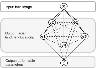
Figure 1: The graphical model. Dashed, dotted, solid lines represent dependencies between pairs of landmarks, landmark and deformable parameters, landmarks and face image, respectively.

Denote the face image as $\mathbf{x}$, the 2D facial landmark locations as $\mathbf{y}$, each landmark is $\mathbf{y}_{i},i=1,\dots,N$. The deformable model parameters that capture pose, identity and expression variation are denoted as $\zeta$. The model parameter we want to learn is denoted as $\Theta$. Assuming $\zeta$ is marginally dependent on $\mathbf{x}$ but conditionally independent of $\mathbf{x}$ given $\mathbf{y}$, the graphical model is shown in Fig. 1.

Based on this definition and assumption, the joint distribution of landmarks $\mathbf{y}$ and deformable parameters $\zeta$ conditioned on the face image $\mathbf{x}$ can be formulated in a CRF framework and written as

$$p_{\Theta}(\mathbf{y},\zeta\mid\mathbf{x})= \frac{1}{Z_{\Theta}(\mathbf{x})}\exp\{-\sum_{i=1}^{N}\phi_{\theta_{1}}(\mathbf{y}_{i},\mathbf{x})$$ (1)

$$-\sum_{i=1}^{N}\sum_{j=i+1}^{N}\psi_{C_{ij}}(\mathbf{y}_{i},\mathbf{y}_{j},\zeta)\}$$

where $\Theta=[\theta_{1},C_{ij}]$, $\theta_{1}$ is neural network parameter, $C_{ij}$ is a $2\times 2$ symmetric positive definite matrix that captures the spatial relationships between a pair of landmark points, $\mathbf{y}_{i}$ and $\mathbf{y}_{j}$. $Z_{\Theta}(\mathbf{x})$ is the partition function. $\phi_{\theta_{1}}(\mathbf{y}_{i},\mathbf{x})$ is the unary energy function with parameter $\theta_{1}$ and $\psi_{C_{ij}}(\mathbf{y}_{i},\mathbf{y}_{j},\zeta)$ is the triple-wise energy function with parameter $C_{ij}$.

3.2 Energy functions

We define the unary and triple-wise energy in Eq.(2) and Eq.(3) respectively.

$$\phi_{\theta_{1}}(\mathbf{y}_{i},\mathbf{x})=\frac{1}{2}[\mathbf{y}_{i}-\mu_{i}(\mathbf{x},\theta_{1})]^{T}\Sigma_{i}^{-1}(\mathbf{x},\theta_{1})[\mathbf{y}_{i}-\mu_{i}(\mathbf{x},\theta_{1})]$$ (2)

$$\psi_{C_{ij}}(\mathbf{y}_{i},\mathbf{y}_{j},\zeta)=[\mathbf{y}_{i}-\mathbf{y}_{j}-\mu_{ij}(\zeta)]^{T}C_{ij}[\mathbf{y}_{i}-\mathbf{y}_{j}-\mu_{ij}(\zeta)]$$ (3)

where $\mu_{i}(\mathbf{x},\theta_{1})$ and $\Sigma_{i}(\mathbf{x},\theta_{1})$ are the outputs of the CNN that represent mean and covariance matrix of each landmark given the image $\mathbf{x}$. $\mu_{ij}(\zeta)$ represents the expected difference between two landmark locations. It is fully determined by the 3D deformable face shape parameters $\zeta$, which contains rigid parameters: rotation $R$ and scale $S$, and non-rigid parameters $\mathbf{q}$. $\begin{bmatrix}\mu_{ij}(\zeta)\\ 1\end{bmatrix}=\frac{1}{\lambda}SR(\bar{\mathbf{y}}_{i}^{3d}+\Phi_{i}\mathbf{q}-\bar{\mathbf{y}}_{j}^{3d}-\Phi_{j}\mathbf{q})$, where $\bar{\mathbf{y}}^{3d}$ is the 3D mean face shape, $\Phi$ is the bases of deformable model, they are learned from data. The deformable parameters $\zeta=[S,R,\mathbf{q}]$ are jointly estimated with 2D landmark locations during inference. In this work, we assume weak perspective projection model. $S$ is a $3\times 3$ diagonal matrix that contains 2 independent parameters $s_{x},s_{y}$ as scaling factor (encode the camera intrinsic parameters) for column and row respectively. While $R$ is a $3\times 3$ orthonormal matrix with 3 independent parameters $\gamma_{1},\gamma_{2},\gamma_{3}$ as the pitch, yaw, roll rotation angle. Note that the translation vector is canceled by taking the difference of two landmark points.

3.3 Learning and Inference

We propose to implement the conditional probability distribution in Eq. (1) with a CNN-CRF model. As shown in Fig. 2, the CNN with parameter $\theta_{1}$ outputs mean $\mu_{i}(\mathbf{x},\theta_{1})$ and covariance matrix $\Sigma_{i}(\mathbf{x},\theta_{1})$ for each facial landmark $\mathbf{y}_{i}$, which together forms the unary energy function $\phi_{\theta_{1}}(\mathbf{y}_{i}\mid\mathbf{x})$. A fully-connected (FC) graph with parameter $C_{ij}\succ 0$ gives the triple-wise energy $\psi_{C_{ij}}(\mathbf{y}_{i},\mathbf{y}_{j},\zeta)$, if given $\zeta$ as well as the output from the unary, the FC can output $\operatorname{E}(\mathbf{x},\zeta,\Theta)$ and $\Lambda_{p}(\mathbf{x},\zeta,\Theta)$, the mean and precision matrix for the conditional distribution $p_{\Theta}(\mathbf{y}\mid\zeta,\mathbf{x})$. The FC can be implemented as another layer following the CNN. Combining the unary and the triple-wise energy, we obtain the joint distribution $p_{\Theta}(\mathbf{y},\zeta\mid\mathbf{x})$. However, direct inference of $\mathbf{y}^{*},\zeta^{*}$ from $p_{\Theta}(\mathbf{y},\zeta\mid\mathbf{x})$ is difficult, therefore we iteratively infer from conditional distributions $p_{\Theta}(\mathbf{y}\mid\zeta,\mathbf{x})$ and $p_{\Theta}(\zeta\mid\mathbf{y})$.

Figure 2: Overall flowchart of the proposed CNN-CRF model.

Mean and Precision matrix
During learning and inference, we need to compute conditional probability $p_{\Theta}(\mathbf{y}\mid\zeta,\mathbf{x})$. By using the quadratic unary and triple-wise energy function, the distribution $p_{\Theta}(\mathbf{y}\mid\zeta,\mathbf{x})$ is a multivariate Gaussian distribution that can be written as

$$p_{\Theta}(\mathbf{y}\mid\zeta,\mathbf{x}) =\frac{1}{Z^{\prime}_{\Theta}(\mathbf{x},\zeta)}\exp\{-\sum_{i=1}^{N}\phi_{\theta_{1}}(\mathbf{y}_{i},\mathbf{x})-\sum_{i=1}^{N}\sum_{j=i+1}^{N}\psi_{C_{ij}}(\mathbf{y}_{i},\mathbf{y}_{j},\zeta)\}$$ (4)

$$=\exp\{\frac{1}{2}\ln{|\Lambda_{p}(\mathbf{x},\Theta,\zeta)|}-\frac{1}{2}[\mathbf{y}-\operatorname{E}(\mathbf{x},\Theta,\zeta)]^{T}\Lambda_{p}(\mathbf{x},\Theta,\zeta)[\mathbf{y}-\operatorname{E}(\mathbf{x},\Theta,\zeta)]\}$$

where $Z^{\prime}_{\Theta}(\mathbf{x})$ is the partition function. $\operatorname{E}(\mathbf{x},\Theta,\zeta)$ and $\Lambda_{p}(\mathbf{x},\Theta,\zeta)$ is the mean and precision matrix of the multivariate Gaussian distribution. They are computed exactly during learning and inference. The mean $E$ can be computed by solving the linear system of equations $\Lambda_{p}E=b$ where $\Lambda_{p}$, the precision matrix, is a symmetric positive definite matrix that can be directly computed from the coefficient in the unary and pairwise term as shown in Eq. (5), and $b$ can be computed from Eq. (5).

$$\Lambda_{p}=\begin{bmatrix}\Lambda_{p11}&\dots&\Lambda_{p1N}\\ \vdots&\ddots&\vdots\\ \Lambda_{pN1}&\dots&\Lambda_{pNN}\\ \end{bmatrix},\,\begin{cases}\Lambda_{pii}=\Sigma_{i}^{-1}+\sum_{j\neq i}C_{ij}\\ \Lambda_{pij}=-C_{ij}\\ \end{cases}b=\begin{bmatrix}b_{1}\\ b_{2}\\ \vdots\\ b_{N}\\ \end{bmatrix},\,b_{i}=\Sigma_{i}^{-1}\mu_{i}+\sum_{j\neq i}C_{ij}\mu_{ij}$$ (5)

From Eq.(5) we can see that the final inference result $E_{i}$ is a combination of $\mu_{i}$ and $\mu_{j}+\mu_{ij},j\in\{1,\dots,N\},j\neq i$. To solve this linear system of equations, we use direct method for exact solution with a fast implementation by Cholesky factorization that requires $\mathcal{O}(N^{3})$ FLOPs. For a practical implementation of the determinant to avoid numerical issues, we again use the Cholesky factorization of $\Lambda_{p}$ to get $LL^{T}=\Lambda_{p}$, then we compute the log determinant by $\ln|\Lambda_{p}|=2\sum\ln diag(L)$ where $diag(\cdot)$ takes the diagonal element of a matrix.

Learning
During learning, our goal is to optimize $\Theta$ given training data $\mathcal{D}=\{\mathbf{x}_{m},\mathbf{y}_{m},m=1,\dots,M\}$. We directly optimize the inference performance. Note that we don’t have ground truth label for $\boldsymbol{\zeta}$, where $\boldsymbol{\zeta}=\{\zeta_{1},\dots,\zeta_{m}\}$. We use an alternating method, based on the current $\Theta^{t},\hat{\mathbf{y}}^{t}=\operatorname{E}(\mathbf{x},\Theta^{t},\zeta^{t})$, optimize $\boldsymbol{\zeta}$ by

$$\zeta^{t+1}_{m} =\mathop{\arg\min}_{\zeta_{m}}-\ln p_{\Theta^{t}}(\hat{\mathbf{y}}^{t}_{m},\zeta_{m}\mid\mathbf{x}_{m})=\mathop{\arg\min}_{\zeta_{m}}\psi_{C_{ij}^{t}}(\hat{\mathbf{y}}^{t}_{mi},\hat{\mathbf{y}}^{t}_{mj},\zeta_{m})$$ (6)

Then based on current $\boldsymbol{\zeta}^{t}$, optimize $\Theta$ by

$$\Theta^{t+1} =\mathop{\arg\min}_{\Theta}Loss=\mathop{\arg\min}_{\Theta}-\sum_{m=1}^{M}\ln p_{\Theta}(\mathbf{y}_{m},\zeta_{m}^{t}\mid\mathbf{x}_{m})=\mathop{\arg\min}_{\Theta}-\sum_{m=1}^{M}\ln p_{\Theta}(\mathbf{y}_{m}\mid\zeta_{m}^{t},\mathbf{x}_{m})$$ (7)

$$=\mathop{\arg\min}_{\Theta}\sum_{m=1}^{M}-\frac{1}{2}\ln{|\Lambda_{p}(\mathbf{x}_{m},\Theta,\zeta_{m}^{t})|}+\frac{1}{2}[\mathbf{y}_{m}-\operatorname{E}(\mathbf{x}_{m},\Theta,\zeta_{m}^{t})]^{T}\Lambda_{p}(\mathbf{x}_{m},\Theta,\zeta_{m}^{t})[\mathbf{y}_{m}-\operatorname{E}(\mathbf{x}_{m},\Theta,\zeta_{m}^{t})]$$

The algorithm for this problem is designed to first set $C_{ij}=\mathbf{0}$ and optimize $\theta_{1}$, the CNN parameter. Then set $C_{ij}=0.01I$ and optimize $\boldsymbol{\zeta}$, then fix a subset of parameters from $\Theta$ and optimize the others alternately, whose pseudo code is shown in Algorithm 1.

Input: training data $\{\mathbf{x}_{m},\mathbf{y}_{m},m=1,\dots,M\}$;

Initialization: parameters $\Theta^{0}=\{\theta_{1}^{0}=randn,C_{ij}^{0}=\mathbf{0}\},t=0$ ;

while not converge do

       $\theta_{1}^{t+1}=\theta_{1}^{t}-\eta_{1}^{t}\frac{\partial Loss}{\partial\theta_{1}}$ ; $t=t+1$;

      

end while

$\hat{\mathbf{y}}^{t}_{m}=\operatorname{E}(\mathbf{x}_{m},\Theta^{t},\zeta^{t})$, $C_{ij}^{t}=0.01I$;

while not converge do

       Stage 1: Fix parameters $\Theta=\Theta^{t}$, optimize $\boldsymbol{\zeta}$ by Eq. (6); $\triangleright$ Optimize deformable parameters

       while not converge do

             $\zeta^{t+1}_{m}=\mathop{\arg\min}_{\zeta_{m}}\psi_{C_{ij}^{t}}(\hat{\mathbf{y}}^{t}_{mi},\hat{\mathbf{y}}^{t}_{mj},\zeta_{m})$, $\hat{\mathbf{y}}^{t+1}=\operatorname{E}(\mathbf{x},\Theta,\zeta^{t+1})$, $t=t+1$;

            

       end while

      $\Theta^{t}=\Theta$

       Stage 2: Fix $\boldsymbol{\zeta}=\boldsymbol{\zeta}^{t},C_{ij}=C_{ij}^{t}$, update $\theta_{1}$ using Eq. (7); $\triangleright$ Update CNN parameters

         while not converge do

             $\theta_{1}^{t+1}=\theta_{1}^{t}-\eta_{1}^{t}\frac{\partial Loss}{\partial\theta_{1}}$ ; $t=t+1$;

            

       end while

        $[\boldsymbol{\zeta}^{t},C_{ij}^{t}]=[\boldsymbol{\zeta},C_{ij}]$

       Stage 3: Fix $\boldsymbol{\zeta}=\boldsymbol{\zeta}^{t},\theta_{1}=\theta_{1}^{t}$, update $C_{ij}$ using Eq. (7); $\triangleright$ Update CRF parameters

         while not converge do

             $C_{ij}^{t+1}=C_{ij}^{t}-\eta_{2}^{t}\frac{\partial Loss}{\partial C_{ij}}$; $t=t+1$;

            

       end while

      $[\boldsymbol{\zeta}^{t},\theta_{1}^{t}]=[\boldsymbol{\zeta},\theta_{1}]$

      

end while

Algorithm 1 Learning CNN-CRF

Inference
The inference problem is a joint inference of $\zeta,\mathbf{y}$ for each input face image $\mathbf{x}$, defined in Eq. (8)

$$\mathbf{y}^{*},{\zeta}^{*}= \mathop{\arg\max}_{\mathbf{y},{\zeta}}\ln p_{\Theta}(\mathbf{y},\zeta\mid\mathbf{x})$$ (8)

We use an alternating method. Based on current $\mathbf{y}^{t}$, optimize $\zeta^{t}$ by (see supplementary):

$$\zeta^{t} =\mathop{\arg\max}_{\zeta}\ln p_{\Theta}(\mathbf{y}^{t},\zeta\mid\mathbf{x})=\mathop{\arg\min}_{\zeta}\sum_{i=1}^{N}\sum_{j=i+1}^{N}\psi_{C_{ij}}(\mathbf{y}_{i}^{t},\mathbf{y}_{j}^{t},\zeta)$$ (9)

Then based on current $\zeta^{t}$, optimize $\mathbf{y}^{t+1}$ by:

$$\mathbf{y}^{t+1} =\mathop{\arg\max}_{\mathbf{y}}\ln p_{\Theta}(\mathbf{y},\zeta^{t}\mid\mathbf{x})=\mathop{\arg\max}_{\mathbf{y}}\ln p_{\Theta}(\mathbf{y}\mid\zeta^{t},\mathbf{x})=\operatorname{E}(\mathbf{x},\Theta,\zeta^{t})$$ (10)

The inference algorithm is shown in Algorithm 2.

Input: face image $\mathbf{x}$

Initialization: $\mathbf{y}_{i}^{0}=\mu_{i},i=1,\dots,N$ , $t=0$;

while not converge do

       Update $\zeta$ by Eq. (9). $\zeta^{t}=\mathop{\arg\min}_{\zeta}\sum_{i=1}^{N}\sum_{j=i+1}^{N}\psi_{C_{ij}}(\mathbf{y}_{i}^{t},\mathbf{y}_{j}^{t},\zeta)$;

       Update $\mathbf{y}$ by Eq. (10). $\mathbf{y}^{t+1}=\operatorname{E}(\mathbf{x},\Theta,\zeta^{t})$;

       $t=t+1$ ;

      

end while

Algorithm 2 Inference for CNN-CRF

4 Experiments

Datasets. We evaluate our methods on popular benchmark facial landmark detection datasets, including 300W (35), Menpo (49), COFW (6), 300VW (1).
300W has 68 landmark annotation. It contains 3837 faces for training and 300 indoor and 300 outdoor faces for testing.
Menpo contains images from AFLW and FDDB with landmark re-annotation following the 68 landmark annotation scheme. It has two subsets, Menpo-frontal which has 68 landmark annotations for near frontal faces (6679 samples) and Menpo-profile which has 39 landmark annotations for profile faces (2300 samples). We use it as a test set for cross dataset evaluation.
COFW has 1345 training samples and 507 testing samples, whose facial images are all partially occluded. The original dataset is annotated with 29 landmarks. We use the COFW-68 test set (19) which has 68 landmarks re-annotation for cross dataset evaluation.
300VW is a facial video dataset with 68 landmarks annotation. It contains 3 scenarios: 1) constrained laboratory and naturalistic well-lit conditions; 2) unconstrained real-world conditions with different illuminations, dark rooms, overexposed shots, etc.; 3) completely unconstrained arbitrary conditions including various illumination, occlusions, make-up, expression, head pose, etc. We use the test set for cross dataset evaluation.
Evaluation metrics. We evaluate our algorithm using the standard normalized mean error (NME) and the Cumulative Errors Distribution (CED) curve. Besides, the area-under-the-curve (AUC) and the failure rate (FR) for a maximum error of 0.07 are reported. Same as in (5), the NME is defined as the average point-to-point Euclidean distance between the ground truth ($\mathbf{y}_{gt}$) and predicted ($\mathbf{y}_{pred}$) landmark locations normalized by the ground truth bounding box size $d=\sqrt{w_{bbox}*h_{bbox}}$, $\text{NME}=\frac{1}{N}\sum_{i=1}^{N}\frac{||\mathbf{y}_{pred}^{(i)}-\mathbf{y}_{gt}^{(i)}||_{2}}{d}$. Based on the NME in the test dataset, we can draw a CED Curve with NME as the horizontal axis and percentage of test images as the vertical axis. Then the AUC is computed as the area under that curve for each test dataset.
Implementation details. To make a fair comparison with the SoA purely deep learning based methods (5), we use the same training and testing procedure for 2D landmark detection. The 3D deformable model was trained on the 300W-train dataset or 300W-LP dataset by structure from motion (4). For CNN, we use 4 stacks of Hourglass with the same structure as (5), each stack followed by a softmax layer to output a probability map for each facial landmark. From the probability map, we compute mean $\mu_{i}$ and covariance $\Sigma_{i}$. And we use additional softmax cross entropy loss and L1 loss on the mean (38) to assist training which shows better performance empirically.
Training procedure: The initial learning rate $\eta_{1}$ is $10^{-4}$ for $15$ epochs using a minibatch of 10, then dropped to $10^{-5}$ and $10^{-6}$ after every 15 epochs and keep training until convergence. The learning rate $\eta_{2}$ is set to $10^{-3}$. We applied random augmentations such as random cropping, rotation, etc. We first train the method on 300W-LP (54) dataset which is augmented from the original 300W dataset for large yaw pose. And then we fine-tune on the original 300W train dataset.
Testing procedure: We follow the same testing procedure as (5). The face is cropped using the ground truth bounding box defined in 300W. The cropped face is rescaled to $256\times 256$ before passed to the network. For the Menpo-profile dataset, the annotation scheme is different, we use the overlapping 26 points for evaluation, i.e., removing points other than the 2 endpoints on the face contour and the eyebrow respectively and removing the 5th point on the nose contour.

4.1 Comparison with existing approaches

1.5	Com.	Chal.	Full
1.2                Inter-ocular distance
MDM (42)	-	-	4.05
RDR (45)	5.03	8.95	5.80
SAN (17)	3.34	6.60	3.98
LAB (4-stack) (44)	2.98	5.19	3.49
Our method (4-stack)	2.93	4.84	3.30
Inter-pupil distance
MDM (42)	4.83	10.14	5.88
LAB (4-stack) (44)	4.20	7.41	4.92
Our method (4-stack)	4.06	6.98	4.63
1.5

Table 1: Comparison with SoA methods on 300W dataset using 300W protocol (NME normalized with inter-ocular/pupil distance %)

In Table 4.1, we compare with some most recent best results reported, in the 300W protocol that trains on LFPW-train, HELEN-train, AFW and tests on LFPW-test, HELEN-test, ibug and use NME normalized with inter-ocular/pupil distance as the metric.

In Table 2, we compare with other baseline facial landmark detection algorithms, including purely deep learning based methods such as TCDCN (50) and FAN (5) as well as hybrid methods such as CLNF (2) and CE-CLM (48). The results for these methods are evaluated using the code provided by the authors in the same experiment protocol, i.e., same bounding box and same evaluation metrics. The CED curves on the 300W testset are shown in Fig. 2(a).

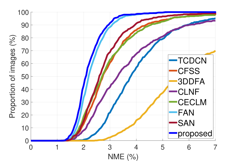
(a) 300W testset

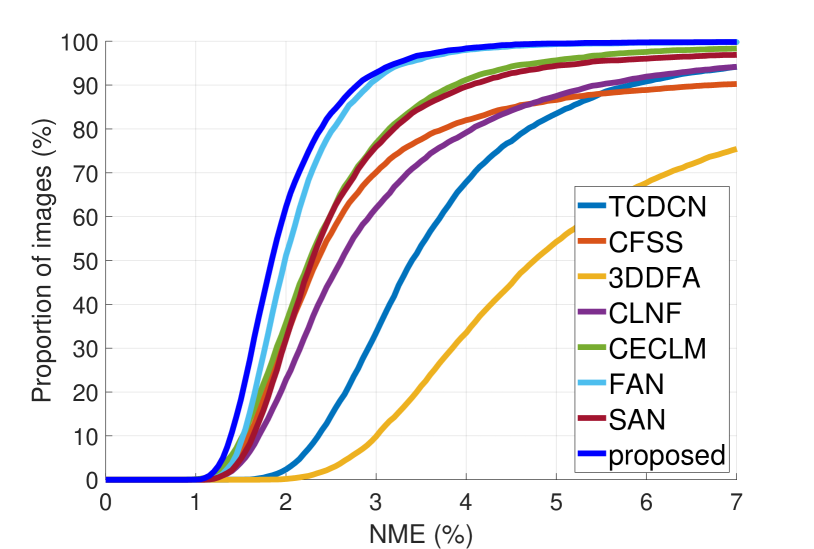
(b) Menpo-frontal dataset

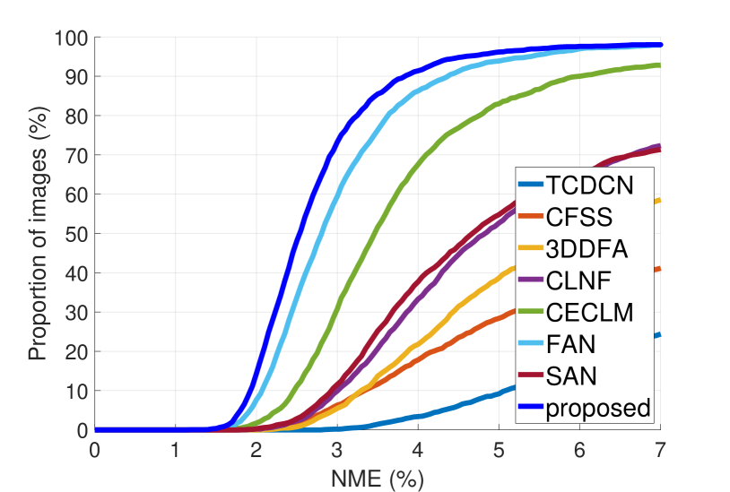
(c) Menpo-profile dataset

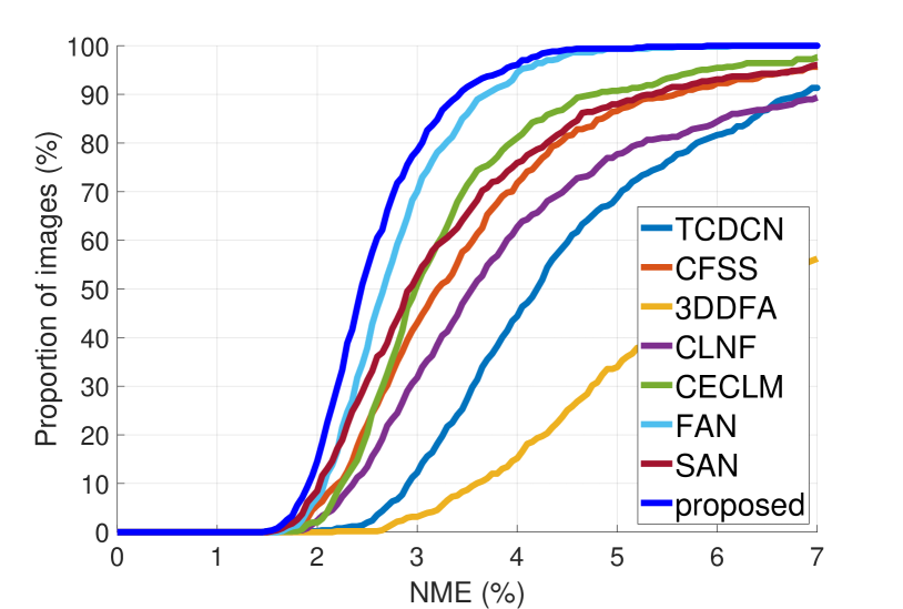
(d) COFW-68 testset

Figure 3: CED curves on different datasets (better viewed in color and magnified)

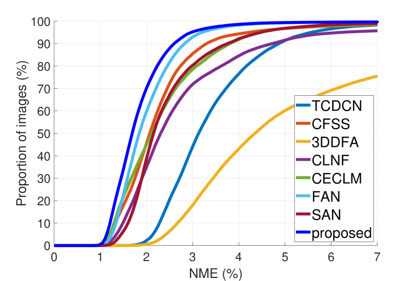
(a) 300VW category1

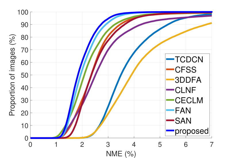
(b) 300VW category2

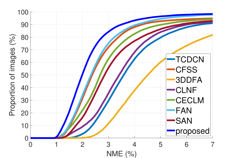
(c) 300VW category3

Figure 4: CED curves on 300VW testset (better viewed in color and magnified)

Cross-dataset Evaluation Besides 300W testset, we evaluate the proposed method on Menpo dataset, COFW-68 testset, 300VW testset for cross dataset evaluation. The results are shown in Table 2 for Menpo and COFW-68 dataset and Table 3 for 300VW dataset. And the CED curves are shown in Fig. 2(b), 2(c), 2(d) respectively. The method is trained on 300W-LP and fine-tuned on 300W Challenge train set for 68 landmarks. We can see that compared to the results on 300W testset and Menpo-frontal dataset, where the SoA methods attaining saturating performance as mentioned in (5), for cross-dataset evaluation in more challenging conditions such as COFW with heavy occlusion and Menpo-profile with large pose, the proposed method shows better generalization ability with a significant performance improvement. On the other hand, the proposed method shows smallest failure rate (FR) on all evaluated datasets.

Table 2: Within and cross dataset prediction results (%)

1.5 Dataset	300W-test			Menpo-frontal			Menpo-profile			COFW-68 test
	NME	AUC	FR	NME	AUC	FR	NME	AUC	FR	NME	AUC	FR
1.2 TCDCN (50)	4.15	42.1	4.83	4.04	46.2	5.84	13.96	5.9	75.61	4.71	35.8	8.68
CFSS (52)	3.09	56.7	1.83	3.91	57.4	9.75	15.04	15.2	58.87	3.79	49.0	4.34
3DDFA (54)	6.90	20.6	30.00	6.57	28.7	24.57	8.37	20.5	41.43	8.13	18.2	43.79
CLNF (2)	4.22	47.6	6.67	3.74	55.4	5.82	8.32	27.8	27.65	4.75	42.9	10.65
CE-CLM (48)	3.05	56.9	2.33	2.78	63.3	1.66	4.63	45.2	7.17	3.36	52.4	2.37
FAN (reported in (5))	-	66.9	-	-	67.5	-	-	-	-	-	-	-
SAN (17)	2.86	59.7	1.00	2.95	61.9	3.11	8.80	29.0	28.65	3.50	51.9	3.94
our method	2.21	68.1	0.17	2.01	71.0	0.16	3.03	60.0	1.96	2.55	63.2	0.00
1.5

Table 3: 300VW testset prediction results for cross-dataset evaluation (%)

1.5 Dataset	300VW-category1			300VW-category2			300VW-category3
	NME	AUC	FR	NME	AUC	FR	NME	AUC	FR
1.2 TCDCN (50)	3.49	51.2	1.74	3.80	45.8	1.76	4.45	43.8	8.85
CFSS (52)	2.44	67.0	1.66	2.49	64.3	0.77	3.26	60.5	5.18
3DDFA (54)	5.80	32.4	24.50	4.44	39.2	8.82	5.48	31.6	18.26
CLNF (2)	3.34	60.4	4.31	2.98	60.0	3.02	4.73	47.1	7.74
CE-CLM (48)	2.54	65.7	1.58	2.39	66.0	0.61	3.61	56.4	5.69
FAN (reported in (5))	-	72.1	-	-	71.2	-	-	64.1	-
SAN (17)	2.58	64.5	1.10	2.57	63.2	0.42	4.06	52.9	7.19
our method	1.91	73.3	0.36	1.97	71.6	0.04	2.50	67.4	1.68
1.5

4.2 Analysis

In this section, we report the results of sensitivity analysis and ablation study. If not specified, analysis is performed on test datasets with models trained on 300W-LP and fine-tuned on 300W train set.

Sensitivity to challenging conditions. We evaluate different methods on challenging conditions caused by either high noise, low resolution, or different initializations in Fig. 5. Generally, the proposed CNN-CRF model is more robust under challenging conditions compared to a pure CNN model with the same structure, i.e. the CNN-CRF model with $C_{ij}=\mathbf{0}$.

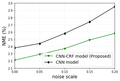
(a) Noise

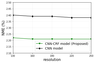
(b) Lower resolution

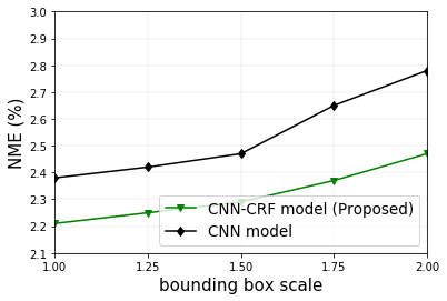
(c) Larger bounding box

Figure 5: Prediction error sensitivity to challenging conditions

Ablation Study. The improvement of the proposed method lies in two aspects. On the one hand, the proposed softmax + L1 mean loss + Gaussian negative log likelihood (NLL) loss gives better results empirically. On the other hand, the joint training of the CNN-CRF model with the assistance of the deformable model captures structured relationships with pose and deformation awareness. To analyze the effect of the proposed method, in Table 4, we evaluate the performance of a plain CNN prediction, the 3D deformable model fitting to the ground truth, and the joint CNN-CRF prediction accuracy.

Table 4: Ablation study on 300W testset (%)

1.5 Method	NME	AUC	FR
1.2 Plain CNN with softmax cross entropy loss	2.38	65.9	0.50
Plain CNN with softmax + L1 mean loss + Gaussian NLL loss (proposed loss)	2.30	67.4	0.50
Separately trained CNN and CRF with proposed loss	2.23	67.8	0.50
Deformable model fitting	1.39	79.8	0.00
Jointly trained CNN-CRF with proposed loss (proposed method)	2.21	68.1	0.17
1.5

5 Conclusion

In this paper, we propose a method combining CNN with a fully-connected CRF model for facial landmark detection. Compared to the state-of-the-art purely deep learning based methods, our method explicitly captures the structured relationships between different facial landmark locations. Compared to previous methods that combine CNN with CRF for human body pose estimation that learn a fixed pairwise relationship representation for different test samples implemented by convolution, our methods capture the structure relationship variations caused by pose and deformation. Moreover, we use a fully-connected model instead of a tree-structured model, obtaining a better representation ability. Lastly, compared to previous methods that do approximate learning such as omitting the partition function and inference such as mean-field method, we perform exact learning and inference, thus able to provide a better structured uncertainty. Experiments on benchmark datasets demonstrate that the proposed method outperforms the existing state-of-the-art methods, in particular under challenging conditions, for both within dataset and cross dataset.

Acknowledgment The work described in this paper is supported in part by NSF award IIS #1539012 and by RPI-IBM Cognitive Immersive Systems Laboratory (CISL), a center in IBM’s AI Horizon Network.

References

- [1] 300VW dataset. http://ibug.doc.ic.ac.uk/resources/300-VW/, 2015.
- [2] Tadas Baltrušaitis, Peter Robinson, and Louis-Philippe Morency. Continuous conditional neural fields for structured regression. In David Fleet, Tomas Pajdla, Bernt Schiele, and Tinne Tuytelaars, editors, Computer Vision – ECCV 2014, pages 593–608, Cham, 2014. Springer International Publishing.
- [3] Yoshua Bengio, Yann LeCun, and Donnie Henderson. Globally trained handwritten word recognizer using spatial representation, convolutional neural networks, and hidden markov models. In J. D. Cowan, G. Tesauro, and J. Alspector, editors, Advances in Neural Information Processing Systems 6, pages 937–944. Morgan-Kaufmann, 1994.
- [4] C. Bregler, L. Torresani, and A. Hertzmann. Nonrigid structure-from-motion: Estimating shape and motion with hierarchical priors. IEEE Transactions on Pattern Analysis and Machine Intelligence, 30(05):878–892, may 2008.
- [5] Adrian Bulat and Georgios Tzimiropoulos. How far are we from solving the 2d & 3d face alignment problem? (and a dataset of 230,000 3d facial landmarks). In International Conference on Computer Vision, 2017.
- [6] Xavier P. Burgos-Artizzu, Pietro Perona, and Piotr Dollár. Robust face landmark estimation under occlusion. In Proceedings of the 2013 IEEE International Conference on Computer Vision, ICCV ’13, pages 1513–1520, Washington, DC, USA, 2013. IEEE Computer Society.
- [7] Xudong Cao, Yichen Wei, Fang Wen, and Jian Sun. Face alignment by explicit shape regression. International Journal of Computer Vision, 107(2):177–190, Apr 2014.
- [8] Dong Chen, Shaoqing Ren, Yichen Wei, Xudong Cao, and Jian Sun. Joint cascade face detection and alignment. In David Fleet, Tomas Pajdla, Bernt Schiele, and Tinne Tuytelaars, editors, Computer Vision – ECCV 2014, pages 109–122, Cham, 2014. Springer International Publishing.
- [9] L. Chen, G. Papandreou, I. Kokkinos, K. Murphy, and A. L. Yuille. Deeplab: Semantic image segmentation with deep convolutional nets, atrous convolution, and fully connected crfs. IEEE Transactions on Pattern Analysis and Machine Intelligence, 40(4):834–848, April 2018.
- [10] Xianjie Chen and Alan Yuille. Articulated pose estimation by a graphical model with image dependent pairwise relations. In Proceedings of the 27th International Conference on Neural Information Processing Systems - Volume 1, NIPS’14, pages 1736–1744, Cambridge, MA, USA, 2014. MIT Press.
- [11] Xiao Chu, Wanli Ouyang, hongsheng Li, and Xiaogang Wang. Crf-cnn: Modeling structured information in human pose estimation. In D. D. Lee, M. Sugiyama, U. V. Luxburg, I. Guyon, and R. Garnett, editors, Advances in Neural Information Processing Systems 29, pages 316–324. Curran Associates, Inc., 2016.
- [12] Xiao Chu, Wanli Ouyang, Hongsheng Li, and Xiaogang Wang. Structured feature learning for pose estimation. In CVPR, 2016.
- [13] T. F. Cootes, G. J. Edwards, and C. J. Taylor. Active appearance models. In Hans Burkhardt and Bernd Neumann, editors, Computer Vision — ECCV’98, pages 484–498, Berlin, Heidelberg, 1998. Springer Berlin Heidelberg.
- [14] T.F. Cootes, C.J. Taylor, D.H. Cooper, and J. Graham. Active shape models-their training and application. Computer Vision and Image Understanding, 61(1):38 – 59, 1995.
- [15] Ciprian A. Corneanu, Meysam Madadi, and Sergio Escalera. Deep structure inference network for facial action unit recognition. In ECCV, 2018.
- [16] Trinh–Minh–Tri Do and Thierry Artieres. Neural conditional random fields. In Yee Whye Teh and Mike Titterington, editors, Proceedings of the Thirteenth International Conference on Artificial Intelligence and Statistics, volume 9 of Proceedings of Machine Learning Research, pages 177–184, Chia Laguna Resort, Sardinia, Italy, 13–15 May 2010. PMLR.
- [17] Xuanyi Dong, Yan Yan, Wanli Ouyang, and Yi Yang. Style aggregated network for facial landmark detection. In Proceedings of the IEEE Conference on Computer Vision and Pattern Recognition (CVPR), pages 379–388, 2018.
- [18] David Eigen, Dilip Krishnan, and Rob Fergus. Restoring an image taken through a window covered with dirt or rain. In Proceedings - 2013 IEEE International Conference on Computer Vision, ICCV 2013, pages 633–640. Institute of Electrical and Electronics Engineers Inc., 2013.
- [19] Golnaz Ghiasi and Charless C. Fowlkes. Occlusion coherence: Detecting and localizing occluded faces. CoRR, abs/1506.08347, 2015.
- [20] R. Girshick, F. Iandola, T. Darrell, and J. Malik. Deformable part models are convolutional neural networks. In 2015 IEEE Conference on Computer Vision and Pattern Recognition (CVPR), pages 437–446, June 2015.
- [21] Max Jaderberg, Karen Simonyan, Andrea Vedaldi, and Andrew Zisserman. Deep Structured Output Learning for Unconstrained Text Recognition. dec 2014.
- [22] V. Jain, J. F. Murray, F. Roth, S. Turaga, V. Zhigulin, K. L. Briggman, M. N. Helmstaedter, W. Denk, and H. S. Seung. Supervised learning of image restoration with convolutional networks. In 2007 IEEE 11th International Conference on Computer Vision, pages 1–8, Oct 2007.
- [23] Amin Jourabloo and Xiaoming Liu. Pose-invariant face alignment via cnn-based dense 3d model fitting. Int. J. Comput. Vision, 124(2):187–203, September 2017.
- [24] F. Kahraman, G. Muhitin, S. Darkner, and R. Larsen. An active illumination and appearance model for face alignment. Turkish Journal of Electrical Engineering and Computer Science, 18(4):677–692, 2010.
- [25] Neeraj Kumar, Peter N. Belhumeur, and Shree K. Nayar. Facetracer: A search engine for large collections of images with faces. In The 10th European Conference on Computer Vision (ECCV), October 2008.
- [26] G. Lin, C. Shen, A. Hengel, and I. Reid. Efficient piecewise training of deep structured models for semantic segmentation. In 2016 IEEE Conference on Computer Vision and Pattern Recognition (CVPR), pages 3194–3203, Los Alamitos, CA, USA, jun 2016. IEEE Computer Society.
- [27] Iain Matthews and Simon Baker. Active appearance models revisited. International Journal of Computer Vision, 60(2):135–164, Nov 2004.
- [28] Stephen Milborrow and Fred Nicolls. Locating facial features with an extended active shape model. In Proceedings of the 10th European Conference on Computer Vision: Part IV, ECCV ’08, pages 504–513, Berlin, Heidelberg, 2008. Springer-Verlag.
- [29] Frederic Morin and Yoshua Bengio. Hierarchical probabilistic neural network language model. In Robert G. Cowell and Zoubin Ghahramani, editors, Proceedings of the Tenth International Workshop on Artificial Intelligence and Statistics, pages 246–252. Society for Artificial Intelligence and Statistics, 2005.
- [30] Alejandro Newell, Kaiyu Yang, and Jia Deng. Stacked hourglass networks for human pose estimation. In Computer Vision - ECCV 2016 - 14th European Conference, Amsterdam, The Netherlands, October 11-14, 2016, Proceedings, Part VIII, pages 483–499, 2016.
- [31] Feng Ning, D. Delhomme, Y. LeCun, F. Piano, L. Bottou, and P. E. Barbano. Toward automatic phenotyping of developing embryos from videos. Trans. Img. Proc., 14(9):1360–1371, September 2005.
- [32] Jian Peng, Liefeng Bo, and Jinbo Xu. Conditional neural fields. In Y. Bengio, D. Schuurmans, J. D. Lafferty, C. K. I. Williams, and A. Culotta, editors, Advances in Neural Information Processing Systems 22, pages 1419–1427. Curran Associates, Inc., 2009.
- [33] Vladan Radosavljevic, Slobodan Vucetic, and Zoran Obradovic. Continuous conditional random fields for regression in remote sensing. In Proceedings of the 2010 Conference on ECAI 2010: 19th European Conference on Artificial Intelligence, pages 809–814, Amsterdam, The Netherlands, The Netherlands, 2010. IOS Press.
- [34] Kosta Ristovski, Vladan Radosavljevic, Slobodan Vucetic, and Zoran Obradovic. Continuous conditional random fields for efficient regression in large fully connected graphs. In AAAI, 2013.
- [35] Christos Sagonas, Epameinondas Antonakos, Georgios Tzimiropoulos, Stefanos Zafeiriou, and Maja Pantic. 300 faces in-the-wild challenge. Image Vision Comput., 47(C):3–18, March 2016.
- [36] J. Saragih and R. Goecke. A nonlinear discriminative approach to aam fitting. In 2007 IEEE 11th International Conference on Computer Vision, pages 1–8, 2007. Exported from https://app.dimensions.ai on 2018/11/15.
- [37] Jason M. Saragih, Simon Lucey, and Jeffrey F. Cohn. Deformable model fitting by regularized landmark mean-shift. International Journal of Computer Vision, 91(2):200–215, Jan 2011.
- [38] Xiao Sun, Bin Xiao, Shuang Liang, and Yichen Wei. Integral human pose regression. arXiv preprint arXiv:1711.08229, 2017.
- [39] Yi Sun, Xiaogang Wang, and Xiaoou Tang. Deep convolutional network cascade for facial point detection. In Computer Vision - CVPR IEEE Computer Society Conference on Computer Vision and Pattern Recognition. IEEE Computer Society Conference on Computer Vision and Pattern Recognition. . 10.1109/CVPR.2013.446., Proceedings, pages 3476–3483, 2013.
- [40] Jonathan Tompson, Ross Goroshin, Arjun Jain, Yann LeCun, and Christoph Bregler. Efficient object localization using convolutional networks. In CVPR, 2015.
- [41] Jonathan Tompson, Arjun Jain, Yann LeCun, and Christoph Bregler. Joint training of a convolutional network and a graphical model for human pose estimation. In Proceedings of the 27th International Conference on Neural Information Processing Systems - Volume 1, NIPS’14, pages 1799–1807, Cambridge, MA, USA, 2014. MIT Press.
- [42] George Trigeorgis, Patrick Snape, Mihalis A. Nicolaou, Epameinondas Antonakos, and Stefanos Zafeiriou. Mnemonic descent method: A recurrent process applied for end-to-end face alignment. In CVPR, pages 4177–4187. IEEE Computer Society, 2016.
- [43] Shih-En Wei, Varun Ramakrishna, Takeo Kanade, and Yaser Sheikh. Convolutional pose machines. In 2016 IEEE Conference on Computer Vision and Pattern Recognition, CVPR 2016, Las Vegas, NV, USA, June 27-30, 2016, pages 4724–4732, 2016.
- [44] Wayne Wu, Chen Qian, Shuo Yang, Quan Wang, Yici Cai, and Qiang Zhou. Look at boundary: A boundary-aware face alignment algorithm. In CVPR, 2018.
- [45] Shengtao Xiao, Jiashi Feng, Luoqi Liu, Xuecheng Nie, Wei Wang, Shuicheng Yan, and Ashraf Kassim. Recurrent 3d-2d dual learning for large-pose facial landmark detection. In The IEEE International Conference on Computer Vision (ICCV), Oct 2017.
- [46] Xuehan Xiong and Fernando De la Torre. Global supervised descent method. In CVPR, pages 2664–2673. IEEE Computer Society, 2015.
- [47] K. Yao, B. Peng, G. Zweig, D. Yu, X. Li, and F. Gao. Recurrent conditional random field for language understanding. In 2014 IEEE International Conference on Acoustics, Speech and Signal Processing (ICASSP), pages 4077–4081, May 2014.
- [48] Amir Zadeh, Yao Chong Lim, Tadas Baltrusaitis, and Louis-Philippe Morency. Convolutional experts constrained local model for 3d facial landmark detection. In The IEEE International Conference on Computer Vision (ICCV) Workshops, Oct 2017.
- [49] S. Zafeiriou, G. Trigeorgis, G. Chrysos, J. Deng, and J. Shen. The menpo facial landmark localisation challenge: A step towards the solution. In 2017 IEEE Conference on Computer Vision and Pattern Recognition Workshops (CVPRW), pages 2116–2125, July 2017.
- [50] Zhanpeng Zhang, Ping Luo, Chen Change Loy, and Xiaoou Tang. Facial landmark detection by deep multi-task learning. In David Fleet, Tomas Pajdla, Bernt Schiele, and Tinne Tuytelaars, editors, Computer Vision – ECCV 2014, pages 94–108, Cham, 2014. Springer International Publishing.
- [51] Shuai Zheng, Sadeep Jayasumana, Bernardino Romera-Paredes, Vibhav Vineet, Zhizhong Su, Dalong Du, Chang Huang, and Philip H. S. Torr. Conditional random fields as recurrent neural networks. In Proceedings of the 2015 IEEE International Conference on Computer Vision (ICCV), ICCV ’15, pages 1529–1537, Washington, DC, USA, 2015. IEEE Computer Society.
- [52] Shizhan Zhu, Cheng Li, Chen Change Loy, and Xiaoou Tang. Face alignment by coarse-to-fine shape searching. In Proceedings of the IEEE Conference on Computer Vision and Pattern Recognition, pages 4998–5006, 2015.
- [53] Shizhan Zhu, Cheng Li, Chen Change Loy, and Xiaoou Tang. Unconstrained face alignment via cascaded compositional learning. 2016 IEEE Conference on Computer Vision and Pattern Recognition (CVPR), pages 3409–3417, 2016.
- [54] Xiangyu Zhu, Zhen Lei, Stan Z Li, et al. Face alignment in full pose range: A 3d total solution. IEEE Transactions on Pattern Analysis and Machine Intelligence, 2017.